uncertainty in qra - on characterisation and methods of...
TRANSCRIPT
LUND UNIVERSITY
PO Box 117221 00 Lund+46 46-222 00 00
Uncertainty in Quantitative Risk Analysis - Characterisation and Methods of Treatment
Abrahamsson, Marcus
Published: 2002-01-01
Link to publication
Citation for published version (APA):Abrahamsson, M. (2002). Uncertainty in Quantitative Risk Analysis - Characterisation and Methods of TreatmentFire Safety Engineering and Systems Safety
General rightsCopyright and moral rights for the publications made accessible in the public portal are retained by the authorsand/or other copyright owners and it is a condition of accessing publications that users recognise and abide by thelegal requirements associated with these rights.
• Users may download and print one copy of any publication from the public portal for the purpose of privatestudy or research. • You may not further distribute the material or use it for any profit-making activity or commercial gain • You may freely distribute the URL identifying the publication in the public portalTake down policyIf you believe that this document breaches copyright please contact us providing details, and we will removeaccess to the work immediately and investigate your claim.

Download date: 16. Jul. 2018

Uncertainty in Quantitative Risk Analysis – Characterisation and Methods of Treatment Marcus Abrahamsson Department of Fire Safety Engineering Lund University, Sweden Brandteknik Lunds tekniska högskola Lunds universitet Report 1024, Lund 2002


Uncertainty in Quantitative Risk Analysis – Characterisation and Methods of Treatment
Marcus Abrahamsson
Lund 2002

Uncertainty in Quantitative Risk Analysis – Characterisation and Methods of Treatment Marcus Abrahamsson Report 1024 ISSN: 1402-3504 ISRN: LUTVDG/TVBB--1024--SE Number of pages: 88 Illustrations: Unless otherwise stated, Marcus Abrahamsson Keywords Quantitative risk analysis, uncertainty analysis, safety, decision making Sökord Kvantitativ riskanalys, osäkerhetsanalys, säkerhet, beslutsfattande Abstract The fundamental problems related to uncertainty in quantitative risk analyses, used in decision making in safety-related issues (for instance, in land use planning and licensing procedures for hazardous establishments and activities) are presented and discussed, together with the different types of uncertainty that are introduced in the various stages of an analysis. A survey of methods for the practical treatment of uncertainty, with emphasis on the kind of information that is needed for the different methods, and the kind of results they produce, is also presented. Furthermore, a thorough discussion of the arguments for and against each of the methods is given, and of different levels of treatment based on the problem under consideration. Recommendations for future research and standardisation efforts are proposed. © Copyright: Brandteknik, Lunds tekniska högskola, Lunds universitet, Lund 2002.
Department of Fire Safety Engineering Lund University
P.O. Box 118 SE-221 00 Lund
Sweden
[email protected] http://www.brand.lth.se/english
Telephone: +46 46 222 73 60
Fax: +46 46 222 46 12
Brandteknik Lunds tekniska högskola
Lunds universitet Box 118
221 00 Lund
[email protected] http://www.brand.lth.se
Telefon: 046 - 222 73 60 Telefax: 046 - 222 46 12
Summary
i
Summary In Sweden, it is possible to discern a considerable increase in the use of quantitative risk analysis (QRA) as part of the foundation for decision making regarding safety-related issues in various areas, for instance land use planning, licensing procedures for hazardous activities, infrastructure projects, and as an integrated part of environmental impact assessments. The QRA methodology has proven to be of substantial use regarding the determination of major contributions to risk, and for the evaluation of different decision options, e.g. different design alternatives. However, due to a lack of consensus concerning which methods, models and inputs should be used in an analysis, and how the, sometimes considerable, uncertainties that will inevitably be introduced during the process should be handled, questions arise regarding the credibility and usability of the absolute results from QRA. Without a description of and discussion on the uncertainties involved in such an analysis, the practical use of the results in absolute terms will be severely limited. For instance, comparison of the results with established risk targets, or tolerability criteria, something that is becoming increasingly common, becomes a fairly arbitrary exercise. The need for standardisation in this area is evident. In this dissertation, the fundamental characteristics of different types of uncertainty introduced in QRA, together with different methods of treatment, are presented. Somewhat simplified, comprehensive uncertainty analysis can be regarded as having three major objectives. Firstly, it is a question of making clear to the decision-maker that we do not know everything, but decisions must be based on what we do know. Secondly, the task is to define how uncertain we are. Is the uncertainty involved acceptable in meeting the decision-making situations we face, or is it necessary to try to reduce the uncertainty in order to be able to place enough trust in the information? Consequently, the third step is to try to reduce the uncertainty involved to an acceptable level. At an elementary level, two major groups of uncertainty can be discerned, i.e. aleatory (or stochastic) and epistemic (or knowledge-based) uncertainty. The most important distinction between these two types of uncertainty, at a practical level, is that the knowledge-based uncertainty can be reduced by further study, should a reduction in the overall uncertainty in the results from an analysis prove necessary. The aleatory uncertainty, on the other hand, is by definition irreducible. Inherent in the QRA process is the need to use expert judgement to estimate the values of unknown parameters (knowledge-based uncertainty). A discussion is presented on various methods of eliciting information from experts in a structured manner, together with a presentation of known pitfalls of such exercises. Knowledge about such procedures, and about the problems associated with them, is a key issue in keeping knowledge-based uncertainty to a minimum. The core of the dissertation, however, is a structured survey of methods of propagating and analysing parameter uncertainty. The basic features of a number of different approaches and methods of uncertainty treatment are presented, followed by a discussion of the arguments for and against the different approaches, and on different levels of treatment based on the problem under consideration. To further exemplify the different features of the methods surveyed, a case study is presented, in which a simplified facility for ammonia storage is analysed with respect to the risk it poses to its surroundings. Emphasis is placed on the kind of information required for use of the different methods, and on the kind of results they produce.
Uncertainty in Quantitative Risk Analysis – Characterisation and Methods of Treatment
ii
It is concluded that methods are available for the explicit treatment of uncertainty in risk analysis with sufficient sophistication for most problems, although some types of uncertainty, mainly those related to completeness and general quality issues, are inherently problematic to quantify. Furthermore it is concluded, regarding future standardisation work in this area, that the probabilistic (Bayesian) framework offers the most comprehensive “tool box” for uncertainty analysis, and appears to be the most promising approach for dealing with the uncertainties in QRA. This is due to its strong theoretical foundations and the possibility of quantifying, and analysing, uncertainties originating from fundamentally different sources (e.g. aleatory and epistemic uncertainty) separately. Recommendations for future research and standardisation efforts in the area are given, and the main conclusion is that generic guidelines across all sectors of industry are not deemed viable, due to the different conditions under which they operate. Instead, differences between various industrial sectors, for instance, the chemical process industry and the transportation industry, would have to be acknowledged in such work, presumably resulting in separate guidelines. Furthermore, possible ways of differentiating the level of uncertainty description and analysis required in an analysis, based on, for instance, the complexity of the problem and the nature of the hazard source, should be examined within each sector of industry. In this dissertation, a discussion is presented on various levels of treatment, which may serve as a basis for further debate. This kind of work on standardisation is an absolute necessity for the general use of risk tolerability criteria to be meaningful.
Sammanfattning
iii
Sammanfattning (summary in Swedish) Användandet av kvantitativ riskanalys som en del av beslutsunderlaget vid ärenden som berör allmänhetens säkerhet i Sverige ökar märkbart, exempelvis inom fysisk planering, tillståndsärenden för farliga verksamheter och i infrastrukturella projekt. Den kvantitativa riskanalysmetodiken har visat sig användbar för att bestämma de huvudsakliga riskbidragen från en verksamhet, samt för att utvärdera och jämföra olika beslutsalternativ, exempelvis olika utformningar av den aktuella anläggningen eller verksamheten, med avseende på risk. En generell avsaknad av samsyn angående vilka metoder, modeller och ingångsdata som bör användas vid sådana analyser, samt angående hur de (ibland mycket stora) osäkerheter som oundvikligen introduceras i riskanalysprocessen skall hanteras, leder emellertid till att den praktiska användbarheten av resultaten i form av absoluta riskmått från en kvantitativ riskanalys kan ifrågasättas. Utan en beskrivning av, och diskussion kring, dessa osäkerheter kommer den reella användbarheten av resultaten att vara mycket begränsad. Exempelvis blir jämförelse av sådana absoluta riskmått med på förhand bestämda kriterier för tolerabel risk, något som blir alltmer vanligt, en tämligen godtycklig övning. Behovet av någon form av standardisering inom området är uppenbart. I denna avhandling presenteras huvudsakliga kännetecken och egenskaper hos olika typer av osäkerhet som uppkommer i en kvantitativ riskanalys, tillsammans med olika metoder för att hantera dessa. Något förenklat kan fullständig analys av osäkerheterna sägas ha tre huvudsakliga syften. I första hand handlar det om att göra klart för de beslutsfattare, som skall använda sig av analysen som beslutsunderlag, att osäkerheten existerar, d.v.s. att det finns saker vi inte vet etc., men beslut måste fattas baserat på det material som finns. I andra hand blir uppgiften att redogöra för hur osäkra vi är. Är nuvarande grad av osäkerhet acceptabel i den aktuella beslutssituationen, eller måste åtgärder vidtas för att minska osäkerheten? Följaktligen blir det tredje huvudsyftet och uppgiften att försöka reducera osäkerheten till en acceptabel nivå. På en grundläggande nivå är det möjligt att särskilja två huvudsaklig typer av osäkerhet. Dessa är osäkerhet i form av naturlig variation (stokastisk osäkerhet) och osäkerhet som härrör sig från avsaknad av kunskap (kunskapsrelaterad osäkerhet, genuin osäkerhet). Den viktigaste skillnaden mellan dessa typer av osäkerhet, på det praktiska planet, är att den kunskapsrelaterade osäkerheten är möjlig att reducera genom vidare studier, medan den stokastiska osäkerheten alltid kommer att finnas där så länge systemet inte ändras. Denna skillnad är givetvis viktig i situationer då bedömningen görs att osäkerheten måste minskas för att ett beslut skall kunna fattas. I situationer av genuin osäkerhet används ofta expertbedömningar för att finna troliga värden på osäkra variabler i en riskanalysmodell. I avhandlingen diskuteras även, i viss utsträckning, olika metoder för att på ett strukturerat sätt inhämta och strukturera information från experter, tillsammans med en presentation av kända svårigheter och fallgropar vid sådana övningar, något som är en förutsättning för att kunna minimera kunskapsrelaterad osäkerhet. Avhandlingens kärna består emellertid av en strukturerad kartläggning av metoder för att fortplanta och analysera osäkerheter i de parametrar och variabler som ingår i riskanalysmodellen. Ett antal olika metoder och angreppssätt presenteras med avseende på deras respektive egenskaper, följt av en diskussion angående argument för och emot de olika metoderna. Även olika nivåer av osäkerhetshantering, baserat på problemets karaktär, komplexitet mm, diskuteras. En case study, där en förenklad anläggning för lagring av
Uncertainty in Quantitative Risk Analysis – Characterisation and Methods of Treatment
iv
ammoniak analyseras med avseende på risk för omgivningen, presenteras i syfte att ytterligare exemplifiera egenskaperna hos de olika metoderna och angreppssätten. Tonvikten ligger här på vilken typ av information som krävs för att använda de olika metoderna, samt vilken typ av resultat de producerar. Slutsatsen dras att metoder för explicit osäkerhetshantering som är tillräckligt sofistikerade för de flesta problemsituationer existerar, även om vissa typer av osäkerhet, ofta relaterade till analysens täckningsgrad och allmänna kvalitetsfrågor, är svåra att kvantifiera. Vad gäller framtida standardiseringsarbete inom området, dras slutsatsen att det probabilistiska (Bayesianska) angreppssättet erbjuder den mest omfattande ”verktygslådan”, samt förefaller vara det mest lovande angreppssättet till hantering av osäkerheter i kvantitativa riskanalyser. Detta främst beroende på dess starka teoretiska överbyggnad samt möjligheten att kvantifiera och analysera osäkerheter från fundamentalt olika källor (exempelvis stokastisk och kunskapsrelaterad osäkerhet) separat i en analys. Rekommendationer ges angående framtida forskning och nationellt standardiseringsarbete på området. De huvudsakliga slutsatserna i detta avseende är att generiska riktlinjer för alla industrisektorer inte bedöms gångbart, främst på grund av genuint olika förutsättningar inom olika sektorer. I stället måste dessa skillnader accepteras, och sektorsspecifika riktlinjer bör tas fram. Vidare bör, inom respektive industrisektor, möjligheten att differentiera kraven på explicit osäkerhetshantering i en analys, baserat på exempelvis det analyserade problemets komplexitet och riskkällans karakteristik undersökas. I rapporten diskuteras olika nivåer av osäkerhetshantering, en diskussion som kan tjäna som underlag för vidare debatt. Denna typ av standardiseringsarbete är en absolut nödvändighet för att en generell användning av kriterier för tolerabel risk skall bli meningsfull.

Table of contents
TABLE OF CONTENTS
SUMMARY.............................................................................................................................................................I
SAMMANFATTNING (SUMMARY IN SWEDISH)......................................................................................III
1. INTRODUCTION........................................................................................................................................ 1 1.1 BACKGROUND ............................................................................................................................................... 1 1.2 OBJECTIVES AND PURPOSE............................................................................................................................. 1 1.3 OVERVIEW OF THE DISSERTATION ................................................................................................................. 2
2. QUANTITATIVE RISK ANALYSIS IN RISK MANAGEMENT ......................................................... 3 2.1 QRA TO DETERMINE MAJOR CONTRIBUTIONS TO RISK................................................................................... 4 2.2 QRA FOR EVALUATING OPTIONS / COMPARATIVE STUDIES............................................................................ 4 2.3 QRA FOR RISK TOLERABILITY DECISIONS...................................................................................................... 4
2.3.1 What is the problem? The ASSURANCE benchmark study................................................................... 5 2.3.2 Possible ways of handling problems associated with absolute measures of risk .................................. 7
2.4 WHY BE EXPLICIT ABOUT UNCERTAINTIES?................................................................................................... 8 3. INTRODUCING UNCERTAINTIES IN THE QRA PROCESS ............................................................ 9
3.1 SOURCES / CLASSES OF UNCERTAINTY ........................................................................................................... 9 3.1.1 Epistemic vs. aleatory uncertainty ........................................................................................................ 9
3.2 UNCERTAINTIES INTRODUCED AT THE DIFFERENT STAGES OF QRA............................................................. 12 3.2.1 The identification stage....................................................................................................................... 12 3.2.2 Frequency estimation.......................................................................................................................... 12
Historical record.......................................................................................................................................................13 Fault and event tree analysis ....................................................................................................................................13
3.2.3 Consequence estimation...................................................................................................................... 14 3.2.4 Estimation of risk ................................................................................................................................ 15
3.3 METHODS OF REPRESENTING UNCERTAINTY................................................................................................ 16 3.3.1 The probabilistic approach................................................................................................................. 16 3.3.2 Interval representation........................................................................................................................ 17 3.3.3 The probability bounds approach ....................................................................................................... 17 3.3.4 Fuzzy representation ........................................................................................................................... 18
3.4 BACKGROUND STUDIES ON METHODS OF CONSIDERING OTHER TYPES OF UNCERTAINTY............................. 19 3.4.1 General quality uncertainty ................................................................................................................ 19 3.4.2 Management and organisational safety .............................................................................................. 19
4. THE USE OF MODELS IN RISK ANALYSIS ...................................................................................... 21 4.1 WHAT AFFECTS THE RELIABILITY OF MODEL PREDICTIONS? ....................................................................... 21
4.1.1 Problem specification ......................................................................................................................... 22 4.1.2 Conceptual and computational model formulation............................................................................. 22 4.1.3 Estimation of parameter values .......................................................................................................... 22 4.1.4 Calculation, presentation and documentation of results..................................................................... 23
4.2 TREATMENT OF MODEL UNCERTAINTY ........................................................................................................ 23 4.2.1 Model validation ................................................................................................................................. 23 4.2.2 Treatment of model uncertainty in the practical situation .................................................................. 24
5. THE USE OF EXPERT JUDGEMENT IN RISK ANALYSIS ............................................................. 27 5.1 GENERAL DISCUSSION ................................................................................................................................. 27 5.2 ELICITATION................................................................................................................................................ 27
5.2.1 Encoding discrete probabilities .......................................................................................................... 27 5.2.2 Encoding continuous probabilities ..................................................................................................... 28 5.2.3 Basic structure of the assessment protocol ......................................................................................... 30

Uncertainty in Quantitative Risk Analysis – Characterisation and Methods of Treatment
5.3 HEURISTICS AND BIASES .............................................................................................................................. 30 5.3.1 Availability.......................................................................................................................................... 31 5.3.2 Anchoring............................................................................................................................................ 31 5.3.3 Representativeness .............................................................................................................................. 32 5.3.4 Control ................................................................................................................................................ 32 5.3.5 Overconfidence and calibration.......................................................................................................... 33
5.4 DIFFERENT APPROACHES TO THE AGGREGATION OF EXPERT OPINIONS ........................................................ 33 6. THE USE OF DATABASES IN RISK ANALYSIS................................................................................ 35
6.1 GENERAL INTRODUCTION ............................................................................................................................ 35 6.2 THE USE OF DATABASES IN THE DIFFERENT STAGES OF AN ANALYSIS .......................................................... 36 6.3 REQUIREMENTS ON DATABASES TO BE USED IN RISK ANALYSIS................................................................... 36
7. METHODS OF PARAMETER UNCERTAINTY PROPAGATION AND ANALYSIS.................... 39 7.1 GENERAL INTRODUCTION ............................................................................................................................ 39
7.1.1 Response surface methods .................................................................................................................. 39 7.2 SENSITIVITY ANALYSIS ................................................................................................................................ 39 7.3 PROBABILISTIC UNCERTAINTY ANALYSIS .................................................................................................... 40
7.3.1 Analytical methods.............................................................................................................................. 41 Approximation from the Taylor series ......................................................................................................................41 First order approximation ........................................................................................................................................42
7.3.2 Sampling methods ............................................................................................................................... 42 Monte Carlo sampling ..............................................................................................................................................43 Latin hypercube sampling .........................................................................................................................................44 Two-phase sampling procedures............................................................................................................................... 45
7.4 INTERVAL ARITHMETIC................................................................................................................................ 47 7.4.1 Worst case analysis requires interval arithmetic ................................................................................ 48 7.4.2 Repeated parameters........................................................................................................................... 48
7.5 PROBABILITY BOUNDS ANALYSIS................................................................................................................. 50 7.6 FUZZY ARITHMETIC ..................................................................................................................................... 51 7.7 ARGUMENTS FOR AND AGAINST THE DIFFERENT APPROACHES TO UNCERTAINTY ANALYSIS ....................... 53
7.7.1 Deterministic (best estimate) approach .............................................................................................. 53 7.7.2 Worst case analysis............................................................................................................................. 53 7.7.3 Interval analysis.................................................................................................................................. 53 7.7.4 Fuzzy arithmetic.................................................................................................................................. 54 7.7.5 Analytical probabilistic analysis......................................................................................................... 54 7.7.6 Monte Carlo analysis (including Latin hypercube and other sampling schemes) .............................. 55 7.7.7 Two-phase Monte Carlo analysis........................................................................................................ 55 7.7.8 Probability bounds analysis................................................................................................................ 55 7.7.9 Computational requirements............................................................................................................... 56 7.7.10 Discussion......................................................................................................................................... 56
7.8 CHOOSING A METHODOLOGY BASED ON THE PROBLEM UNDER CONSIDERATION ......................................... 56 8. METHODS OF RANKING UNCERTAIN PARAMETERS................................................................. 59
8.1 ANALYTICAL METHODS ............................................................................................................................... 59 8.2 NUMERICAL METHODS................................................................................................................................. 59
8.2.1 Correlation coefficients....................................................................................................................... 59 8.2.2 Partial correlation coefficients ........................................................................................................... 60 8.2.3 Multiple linear regression analysis..................................................................................................... 60
Partial regression coefficients ..................................................................................................................................61 Standardised partial regression coefficients .............................................................................................................61
8.2.4 Rank correlation coefficients .............................................................................................................. 61

Table of contents
9. A CASE STUDY ........................................................................................................................................ 63 9.1 EXTENDED QRA - DEFINITION OF POSSIBLE INCIDENTS/SCENARIOS............................................................ 64 9.2 CONCENTRATION AT GRID POINT (300,0)..................................................................................................... 64
9.2.1 A single LOC....................................................................................................................................... 64 The Dutch approach .................................................................................................................................................65 Interval analysis approach........................................................................................................................................65 Fuzzy arithmetic approach........................................................................................................................................66 The Monte Carlo approach.......................................................................................................................................67 Probability bounds approach....................................................................................................................................69 Comparison of the results .........................................................................................................................................70
9.2.2 Model uncertainty – two-phase Monte Carlo ..................................................................................... 71 9.3 INDIVIDUAL RISK AT GRID POINT (300,0) ..................................................................................................... 72
9.3.1 Ranking the uncertain parameters ...................................................................................................... 74 9.4 SOCIETAL RISK IN GRID CELL (300,0)........................................................................................................... 75 9.5 CONCLUSIONS FROM THE CASE STUDY ........................................................................................................ 76
10. CONCLUSIONS AND RECOMMENDATIONS ................................................................................... 77 10.1 CONCLUSIONS DRAWN FROM THE STUDY................................................................................................... 77 10.2 RECOMMENDATIONS ON FUTURE RESEARCH AND STANDARDISATION EFFORTS......................................... 78
ACKNOWLEDGEMENTS ................................................................................................................................ 81
REFERENCES .................................................................................................................................................... 83 DATABASES....................................................................................................................................................... 83 GENERAL REFERENCES ..................................................................................................................................... 83
APPENDICES ..................................................................................................................................................... 89 APPENDIX 1 EXAMPLES OF EXISTING DATABASES.......................................................................................... 89
A.1.1 Accident (event) databases ................................................................................................................. 89 MHIDAS (Major Hazard Incident Data Service)......................................................................................................89 FACTS (Failure and Accident Technical Information System) .................................................................................89 The Accident Database .............................................................................................................................................90 MARS (Major Accident Reporting System) ...............................................................................................................90
A.1.2 Failure frequency databases............................................................................................................... 91 OREDA .....................................................................................................................................................................91 Guidelines for Process Equipment Reliability Data – With Data Tables..................................................................91
APPENDIX 2 BACKGROUND STUDIES ON COMPLETENESS AND GENERAL QUALITY UNCERTAINTY ............ 93 A.2.1 Description of uncertainty in quantitative risk analysis ..................................................................... 93
Classification of uncertainty .....................................................................................................................................94 Best estimate / uncertainty in the best estimate.........................................................................................................94 Determination of uncertainty factors in the different classes....................................................................................95 Conclusions...............................................................................................................................................................96
APPENDIX 3 BACKGROUND INFORMATION ON THE CASE STUDY .................................................................... 97 A.3.1 Models and basic assumptions ........................................................................................................... 97
Mass discharge rate ..................................................................................................................................................97 Vapour cloud dispersion ...........................................................................................................................................97 Probit equations........................................................................................................................................................98
A.3.3 Specification of uncertain parameters................................................................................................ 99 A.3.4 Example file from RiskCalc .............................................................................................................. 101

Uncertainty in Quantitative Risk Analysis – Characterisation and Methods of Treatment

Introduction
1
1. Introduction
1.1 Background The role of Quantitative Risk Analysis (QRA) as a foundation for decision making regarding hazardous activities and establishments, has gained increased importance during recent decades. In Sweden, it is possible to discern an increase of the use of QRA in various decision-making situations where safety issues are of major concern, for instance in land use planning, licensing procedures for hazardous establishments, infrastructure projects, the transportation of hazardous goods, and as part of environmental impact assessments. In a study by Abrahamsson (to be published during the summer of 2002), where some twenty risk analysis reports from the areas mentioned above were studied, one of the major findings was the significant diversity regarding approaches, methods, models and general assumptions applied in the analyses. This might pose a serious problem in practical decision-making situations since analyses based on different methods, models and basic assumptions will be difficult to compare. Also, a general lack of transparency of the analyses makes them difficult to verify and reproduce for anyone not involved in the work; a definite drawback for e.g. the authorities who are to review and evaluate the results of such analyses. In Sweden no standard for risk analysis is currently recommended, a situation that contributes to the diversity of approaches used, even within specific sectors of industry. The need for work in this area is evident. The problem of acknowledging and treating uncertainty is central for the quality and practical usability of quantitative risk analysis. When performing a QRA, a wide range of uncertainties will inevitably be introduced during the process. The impact of these uncertainties must somehow be addressed if the analysis is to serve as a tool in the decision-making process. In Abrahamsson (2000), a study of international standards for risk analysis is presented. One of the major conclusions of the study was that all of the standards considered acknowledged the importance of explicit and careful treatment of uncertainties while performing quantitative risk analysis, even though none of them offered any explicit information on how this should be done in practice. A starting point for this dissertation is that any standardisation recommendations in this area will have to be explicit regarding the treatment of uncertainty in the QRA process.
1.2 Objectives and purpose The main objective of the work described in this dissertation was to provide background material for future standardisation efforts regarding quantitative risk analysis for use in safety-related decision making in Sweden. Regarding the dissertation itself, the principal objectives are twofold: firstly, to clarify the fundamental problems uncertainty poses for risk analysis in decision making, and secondly to provide a structured survey of the approaches and methods available for dealing with these problems.

Uncertainty in Quantitative Risk Analysis – Characterisation and Methods of Treatment
2
1.3 Overview of the dissertation In Chapter 2 the role of quantitative risk analysis in risk management is discussed. Different objectives of QRA are described, with emphasis on the use of QRA for risk tolerability decisions, since this aspect poses the most intricate problems regarding uncertainty due to the use of absolute estimates of risk. To illustrate the main problems introduced by uncertainties in quantitative risk analyses, some results from the European benchmark study ASSURANCE are briefly introduced and discussed. In Chapter 3 a discussion on major sources/classes of uncertainty is presented, together with an overview of how different types of uncertainties might be introduced in different stages of the QRA process. Furthermore, different methods of representing uncertainty regarding parameters and variables used in risk modelling are briefly introduced, followed by a concise presentation of methods of considering “general quality uncertainty”, and methods of incorporating managerial and organisational issues in a QRA. The main theme of Chapter 4 is the treatment of model uncertainty. An outline of what might affect the reliability of model predictions is given, followed by a discussion on the handling of model uncertainty in the practical risk analysis situation. One of the major challenges in quantitative risk analysis is the persistent lack of data, making the use of expert judgement to provide estimates of unknown quantities a necessity. In Chapter 5 some widely used approaches to expert elicitation are presented together with a discussion on some of the many known pitfalls of such exercises. The chapter is concluded with a brief presentation of three different approaches for the aggregation of expert opinions. Chapter 6 contains a brief introduction to how different kinds of experience (accident) databases might be of use in different stages of the QRA process. In addition, some basic requirements on databases to be used in risk analysis are given. While searching the literature in this area I have come to realise that there is an abundant variety of methods available for parameter uncertainty analysis. In Chapter 7 a comprehensive presentation of various methods is given, focusing on the kind of information necessary for the use of the different methods, and the kind of results they produce. Furthermore, arguments for and against the different approaches are presented, together with a discussion on different levels of treatment of uncertainty based on the problem under consideration. One of the major objectives of performing a complete parameter uncertainty analysis is that it enables the analyst to rank the parameters with respect to their contributions to the overall uncertainty in the model prediction. In Chapter 8, a fairly thorough presentation of different methods of ranking the uncertain parameters in a model is given. Chapter 9 presents a theoretical case study, where the different methods for uncertainty analysis are used in a simplified case. This is followed by conclusions and recommendations for future research and standardisation efforts in Chapter 10.
Quantitative risk analysis in risk management
3
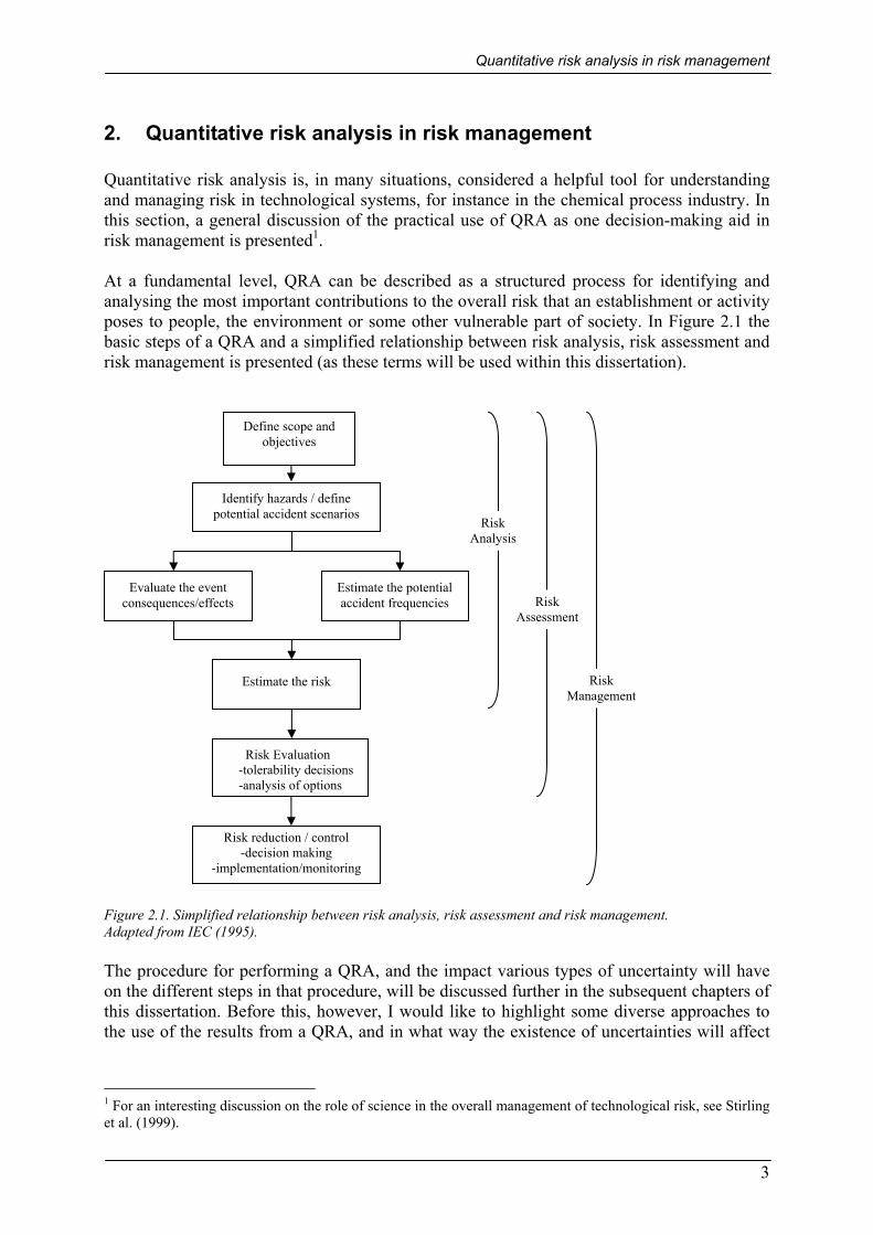
2. Quantitative risk analysis in risk management Quantitative risk analysis is, in many situations, considered a helpful tool for understanding and managing risk in technological systems, for instance in the chemical process industry. In this section, a general discussion of the practical use of QRA as one decision-making aid in risk management is presented1. At a fundamental level, QRA can be described as a structured process for identifying and analysing the most important contributions to the overall risk that an establishment or activity poses to people, the environment or some other vulnerable part of society. In Figure 2.1 the basic steps of a QRA and a simplified relationship between risk analysis, risk assessment and risk management is presented (as these terms will be used within this dissertation).
Figure 2.1. Simplified relationship between risk analysis, risk assessment and risk management. Adapted from IEC (1995). The procedure for performing a QRA, and the impact various types of uncertainty will have on the different steps in that procedure, will be discussed further in the subsequent chapters of this dissertation. Before this, however, I would like to highlight some diverse approaches to the use of the results from a QRA, and in what way the existence of uncertainties will affect
1 For an interesting discussion on the role of science in the overall management of technological risk, see Stirling et al. (1999).
Identify hazards / define potential accident scenarios
Evaluate the event consequences/effects
Estimate the potential accident frequencies
Estimate the risk
Risk Evaluation -tolerability decisions -analysis of options
Risk reduction / control -decision making
-implementation/monitoring
Risk Analysis
Risk Assessment
Risk Management
Define scope and objectives
Uncertainty in Quantitative Risk Analysis – Characterisation and Methods of Treatment
4
the credibility and usefulness of these results. This discussion is related to the “Risk evaluation” box in Figure 2.1.
2.1 QRA to determine major contributions to risk A key merit of QRA is that the procedure provides a structured way to determine the major contributions to the overall risk, which will obviously prove useful in the risk management situation where decisions are to be made regarding efforts to reduce the risk. Knowing the major contributions to the overall risk is really a prerequisite for being able to direct efforts towards managing and reducing the risk to those areas where they will have the greatest impact, thus facilitating cost effectiveness in risk management (Hendershot, 1995).
2.2 QRA for evaluating options / comparative studies It has been stated that QRA is most useful when used to evaluate the impact of design alternatives on facility risk (comparing the risk of one design option with one or more alternatives) (Hendershot, 1995). Although this particular statement referred to QRA performed in a chemical process industry context, the merits of QRA for comparative studies and for evaluating competing options are valid in a more general sense, for instance in land use planning with a variety of hazard sources. As stated in CCPS (2000, p. 450): “The use of risk estimates in a relative sense is often much less sensitive to error. /…/ Because the same methodologies and assumptions are used to the extent possible to evaluate the various alternatives under consideration, the resulting risk estimates are subject to similar uncertainties. Thus, the relative ranking of the various alternatives may be less affected by uncertainty than the absolute value of the risk measure”. A condition for this statement is that the alternatives really are highly comparable, e.g. a comparison of two alternative locations of a new road through the outskirts of a city. In situations where the alternatives are not entirely comparable, e.g. comparison of the risks associated with the transport of dangerous goods from point A to point B via railroad and road transport, one would have to be more careful regarding the impact of uncertainties since the methods of arriving at an estimate of the risks involved might be quite different for the two transportation alternatives.
2.3 QRA for risk tolerability decisions Due to the fact that a QRA will produce a quantitative estimate of the risks generated by an activity or establishment, it is inevitable that questions will be raised as to whether this level of risk is to be considered tolerable. As a consequence of this, several companies, organisations, authorities and even countries have issued their own “target risks” or criteria for what may be considered tolerable levels of risk. Issues regarding the suitability of such tolerability criteria, and the problems related to establishing them, will not be discussed at length here. However, since they inherently focus on absolute risk levels, the impact of uncertainties will play a major role in the usefulness of such criteria. For a survey of existing criteria and a structured discussion regarding the basic features of such criteria and underlying principles see, for instance, Davidsson et al. (1997). In Sweden, no such criteria for the tolerability of risk have been issued at the national level. However, local authorities are beginning to use their own, for instance, in planning situations,

Quantitative risk analysis in risk management
5
and there is a general trend where a growing group of actors in the decision-making process, e.g. in land use planning, are advocating such an approach. This development is not unproblematic, however. Depending on how one makes use of such criteria2, this could lead to problems since there is still a great deal of confusion in the Swedish risk analysis community regarding methods, models and data to be used in a QRA. No standard for risk analysis is currently available in Sweden. 2.3.1 What is the problem? The ASSURANCE benchmark study Several studies have been undertaken during the past decade regarding the impact of uncertainty on the results of quantitative risk analyses. In a benchmark exercise on major hazard analysis for a chemical plant, managed by the Joint Research Centre (JRC) during 1988-1990, 11 teams from different European countries performed an analysis for a reference object, an ammonia storage facility (Amendola et al., 1992). The objectives of the study were to evaluate the state of the art and to obtain estimates of the degree of uncertainty in risk studies. The results of this study showed great variability in risk estimations between the different analysis teams. A follow-up benchmark exercise, ASSURANCE (ASSessment of Uncertainties in Risk ANalysis of Chemical Establishments), which was completed in late 2001, where seven teams from different European countries performed a risk analysis on an ammonia storage facility, showed a similar considerable spread in both the frequency and the consequence assessment, suggesting that consensus on methodologies, models and basic assumptions has not been reached. In this section, some of the results from the ASSURANCE study will be presented to exemplify the problems encountered in decision making based on absolute risk measures. An important part of the study was to ask the seven teams to perform an analysis of 11 “reference scenarios”, which were selected partly in order to cover different release and dispersion conditions. The scenarios chosen for the analysis were:
1. Major ammonia leak from an 8´´ feeding pipe (a long pipeline connected to a pump, containing pressurised ammonia)
2. Breakage of a 4´´ pipe (connecting the cryogenic with the pressurised storage area) 3. Rupture or disconnection between ammonia transport ship and unloading arm
(refrigerated ammonia) 4. Rupture of a 10´´ pipe (discharge line, tank to ship; refrigerated ammonia) 5. Rupture of a ship tank (release of refrigerated ammonia on the sea surface) 6. Catastrophic rupture of a cryogenic tank 7. Rupture of a 20´´ pipe connected to the cryogenic tank (refrigerated ammonia) 8. Catastrophic rupture of one of the ten pressurised tanks 9. Rupture of a 4´´ pipe on the distribution line (pressurised ammonia) 10. Rupture or disconnection between truck and unloading arm (pressurised ammonia) 11. Catastrophic rupture of a truck tank
For these 11 reference scenarios, both frequency and consequence calculations were performed. The spread in the results is shown in Table 2.1 and Figure 2.2.
2 In a context where target risks, or tolerability criteria, are used in a “clear cut” manner (i.e. either you pass or you fail), problems arise due to lack of consensus regarding methods, models and which data to use in the QRA.
Uncertainty in Quantitative Risk Analysis – Characterisation and Methods of Treatment
6
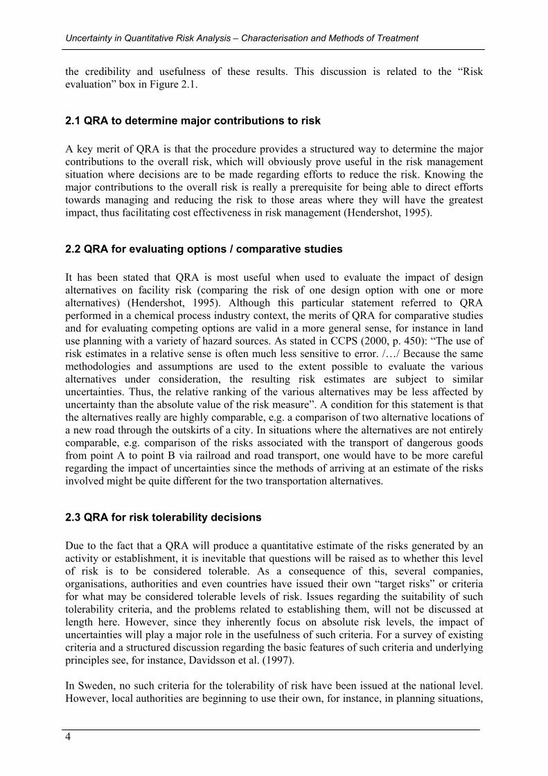
Table 2.1. Frequencies of the top events of the common scenarios assessed by the partners (events/year). From Lauridsen et al. (2001b).
Table 2.1 shows that the range of deviation for several of the reference scenarios covers several orders of magnitude; a spread in the results that will obviously be transferred to the final risk estimates (partner 6 did not provide estimates of frequencies). For more information on the principal methods of frequency calculation used by the different partners, see Lauridsen et al. (2001b).
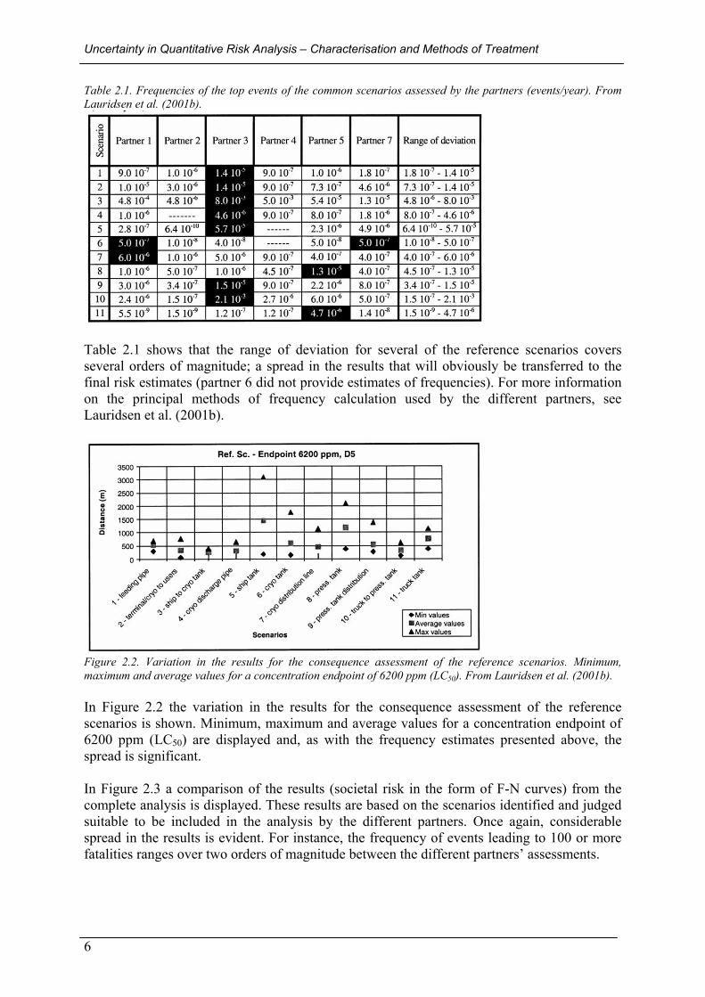
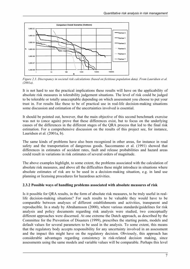
Figure 2.2. Variation in the results for the consequence assessment of the reference scenarios. Minimum, maximum and average values for a concentration endpoint of 6200 ppm (LC50). From Lauridsen et al. (2001b). In Figure 2.2 the variation in the results for the consequence assessment of the reference scenarios is shown. Minimum, maximum and average values for a concentration endpoint of 6200 ppm (LC50) are displayed and, as with the frequency estimates presented above, the spread is significant. In Figure 2.3 a comparison of the results (societal risk in the form of F-N curves) from the complete analysis is displayed. These results are based on the scenarios identified and judged suitable to be included in the analysis by the different partners. Once again, considerable spread in the results is evident. For instance, the frequency of events leading to 100 or more fatalities ranges over two orders of magnitude between the different partners’ assessments.
Quantitative risk analysis in risk management
7
Figure 2.3. Discrepancy in societal risk calculations (based on fictitious population data). From Lauridsen et al. (2001a). It is not hard to see the practical implications these results will have on the applicability of absolute risk measures in tolerability judgement situations. The level of risk could be judged to be tolerable or totally unacceptable depending on which assessment you choose to put your trust in. For results like these to be of practical use in real-life decision-making situations some discussion and estimation of the uncertainties involved is essential. It should be pointed out, however, that the main objective of this second benchmark exercise was not to (once again) prove that these differences exist, but to focus on the underlying causes of the differences in the different stages of the QRA process that led to the final risk estimation. For a comprehensive discussion on the results of this project see, for instance, Lauridsen et al. (2001a, b). The same kinds of problems have also been recognized in other areas, for instance in road safety and the transportation of dangerous goods. Saccomanno et al. (1991) showed that differences in estimates of accident rates, fault and release probabilities and hazard areas could result in variations in risk estimates of several orders of magnitude. The above examples highlight, to some extent, the problems associated with the calculation of absolute risk measures, and above all the difficulties these might introduce in situations where absolute estimates of risk are to be used in a decision-making situation, e.g. in land use planning or licensing procedures for hazardous activities. 2.3.2 Possible ways of handling problems associated with absolute measures of risk Is it possible for QRA results, in the form of absolute risk measures, to be truly useful in real-life decision-making situations? For such results to be valuable they would have to be comparable between analyses of different establishments and activities, transparent and reproducible. In a study by Abrahamsson (2000), where various standards/guidelines for risk analysis and policy documents regarding risk analysis were studied, two conceptually different approaches were discerned. At one extreme the Dutch approach, as described by the Committee for the Prevention of Disasters (1999), prescribes the starting points, models and default values for several parameters to be used in the analysis. To some extent, this means that the regulatory body accepts responsibility for any uncertainty involved in an assessment and the impact this might have on the regulatory decision. Obviously, this approach has considerable advantages regarding consistency in risk-related decision making, since assessments using the same models and variable values will be comparable. Perhaps this level

Uncertainty in Quantitative Risk Analysis – Characterisation and Methods of Treatment
8
of standardisation of the risk analysis process is required for the explicit use of target risks or tolerability criteria to make sense. On the other hand, it is my firm belief that this approach might have negative effects on scientific progress regarding the development of new models for use in risk assessment, as well as a risk assessor’s motivation for finding situation-specific data to use in his/her analysis. It should be mentioned however, that the Dutch guideline encourages the development of situation-specific models and the use of site-specific data, as long as the deviations from the prescribed models and data are explicitly explained and justified for the authorities concerned. As stated before, it seems to me that the objective of this guideline is to make it possible to make consistent decisions, and not to try to be explicit about uncertainty in the analyses. At the other extreme, the American Environmental Protection Agency (EPA) policy for the use of probabilistic analysis in risk assessment (U.S. EPA, 1997) advocates a somewhat different approach. It focuses more on providing conditions to be met in an assessment to ensure high-quality science, regarding transparency, reproducibility, and the use of sound methods. It also recognizes the fact that there are situations where a fully probabilistic approach is not called for, and it provides guidance on how to decide whether to perform a QRA or not. The strength of this approach, from a scientific point of view, is that it does not dictate any specific method or methods, but highlights the importance of transparency and of being explicit about the methods and input used in an assessment. From a decision-maker’s point of view, however, this approach is more demanding than, for instance, the Dutch approach, since clear-cut target risks will be difficult to apply and one will have to turn to other “softer” means of evaluating the results from a QRA. For an approach like the one adopted by the EPA to be successful it is vital to define methods for characterizing, quantitatively, the variability and uncertainty of a risk estimate, to identify the main sources of variability and uncertainty, and their relative contributions to the overall uncertainty in the results. This task is one of the major objectives of the present work.
2.4 Why be explicit about uncertainties? It should be clear from the above discussion that uncertainties are ever present in the QRA process and will by definition affect the practical usefulness of the results. In Chapter 3, the different parts of the QRA process will be further examined, and various kinds of uncertainties introduced at different stages of that process will be described and discussed. Before that, however, I would like to present my simplified view on the primary objectives for being explicit about uncertainties. “One could regard uncertainty analysis as having three fundamental purposes. Firstly, it is a question of making clear to the decision maker that we do not know everything, but decisions has to be based on what we have. Secondly, the task is to try to define how uncertain we are. Is the uncertainty involved acceptable in meeting the decision-making situations we face, or is it necessary to try to reduce the uncertainty in order to be able to place enough trust in the information? Consequently, the third step is to try to reduce the uncertainty involved to an acceptable level.” (Abrahamsson, 2000).
Introducing uncertainties in the QRA process
9
3. Introducing uncertainties in the QRA process
3.1 Sources / classes of uncertainty To help understand the concept of uncertainty, and to be able to treat uncertainties in a structured manner, many attempts have been made to characterise classes of uncertainty and the underlying sources of uncertainty. In this section a brief summary of classes/sources of uncertainty found in literature is presented. In Parry (1998) the perhaps most traditional definition of classes of uncertainty is presented. The three major groups of uncertainty, according to this definition, are:
• parameter uncertainty • model uncertainty • completeness uncertainty
Parameter uncertainty, which is introduced when the values of the parameters used in the models are not accurately known, is often dealt with by assigning probability distributions or some other kind of distribution to the parameters, representing the analyst’s knowledge about them. Parameters used in a model may also be subject to natural variability, which may be dealt with the same way. (More on the distinction between knowledge-based uncertainty and variability can be found in Section 3.1.1.) An array of methods for representing and propagating parameter uncertainty in risk analysis models is presented in Chapter 7. Model uncertainty arises from the fact that any model, conceptual or mathematical, will inevitably be a simplification of the reality it is designed to represent (for an explicit discussion on model uncertainty, see Chapter 4), whereas completeness uncertainty originates from the fact that not all contributions to risk are addressed in QRA models. For example, it will not be feasible to cover all possible initiating events in a QRA. Knowing the sources of uncertainty involved in the analysis plays an important role in the overall handling of uncertainty. First of all, different kinds of uncertainty call for different methods of treatment. Another aspect is the possibility of reducing uncertainty. If one knows why there are uncertainties and what kinds of uncertainty are involved, one has a better chance of finding the right methods for reducing them. 3.1.1 Epistemic vs. aleatory uncertainty At an even more fundamental level, two major groups of uncertainty are recognised in most of the literature. On the one hand there is the aleatory, or stochastic, uncertainty and on the other the epistemic, or knowledge-based uncertainty. This section provides a brief discussion on the differences and practical meaning of these two types of uncertainty. The question arises: can uncertainty just be considered as uncertainty regardless of its origin? Is there really a need to identify and separate various kinds of uncertainty? The answers to these questions are yes and no, respectively. As stated by Winkler (1996): ”At a fundamental level, uncertainty is uncertainty, yet the distinctions are related to very important practical aspects of modelling and obtaining information. Such aspects include decomposition in model building, bounding models, identification and incorporation of different types of information,

Uncertainty in Quantitative Risk Analysis – Characterisation and Methods of Treatment
10
probability assessment, value of information, and sensitivity analysis.” There is no fundamental reason for distinguishing between different types of uncertainty, but it may well be appropriate in many practical applications. The most widespread tool (but not the only tool, as will be discussed further in Chapter 7,) for quantifying uncertainties is the mathematical concept of probability. Unfortunately, the concept of probability has no unequivocal definition. The two main schools of thought in this field are the frequentist and the Bayesian. According to Paté-Cornell (1996) the frequentist school (including classical statisticians), defines probability as a limiting frequency, which applies only if one can identify a sample of independent, identically distributed observations of the phenomenon of interest. The Bayesian school, on the other hand, regards the concept of probability as a degree of belief. This means that not only statistical data and physical models will serve as information, but also expert opinions which will, by nature, be subjective. The Bayesian framework also provides methods of updating probabilities when new data are introduced. The type of uncertainty here referred to as aleatory, has been given many different names in the literature, e.g. variability, randomness, stochastic or irreducible uncertainty. Significant for aleatory uncertainty is that it represents randomness in nature and that it is only in the domain of this type of uncertainty that the frequentist definition of probability is valid.
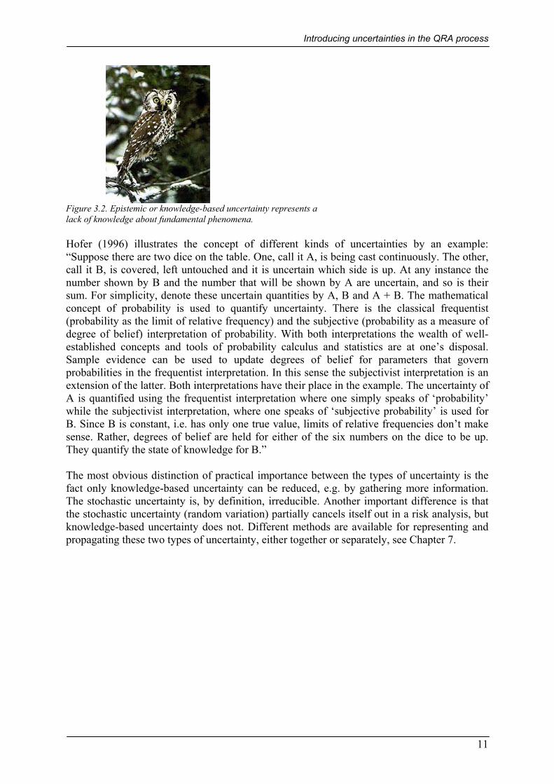
Figure 3.1. Aleatory or stochastic uncertainty represents randomness in nature, e.g. wind speed. As with the aleatory uncertainty described above, epistemic uncertainty has many aliases, e.g. ambiguity, ignorance, knowledge-based, reducible or subjective uncertainty. In essence, epistemic uncertainty represents a lack of knowledge about fundamental phenomena. It is when dealing with this kind of uncertainty that one often has to rely on experts and their subjective judgement. Different techniques for eliciting information from subjective opinions given by experts, together with a discussion of some possible pitfalls, are more thoroughly discussed in Chapter 5.
Introducing uncertainties in the QRA process
11
Figure 3.2. Epistemic or knowledge-based uncertainty represents a lack of knowledge about fundamental phenomena. Hofer (1996) illustrates the concept of different kinds of uncertainties by an example: “Suppose there are two dice on the table. One, call it A, is being cast continuously. The other, call it B, is covered, left untouched and it is uncertain which side is up. At any instance the number shown by B and the number that will be shown by A are uncertain, and so is their sum. For simplicity, denote these uncertain quantities by A, B and A + B. The mathematical concept of probability is used to quantify uncertainty. There is the classical frequentist (probability as the limit of relative frequency) and the subjective (probability as a measure of degree of belief) interpretation of probability. With both interpretations the wealth of well-established concepts and tools of probability calculus and statistics are at one’s disposal. Sample evidence can be used to update degrees of belief for parameters that govern probabilities in the frequentist interpretation. In this sense the subjectivist interpretation is an extension of the latter. Both interpretations have their place in the example. The uncertainty of A is quantified using the frequentist interpretation where one simply speaks of ‘probability’ while the subjectivist interpretation, where one speaks of ‘subjective probability’ is used for B. Since B is constant, i.e. has only one true value, limits of relative frequencies don’t make sense. Rather, degrees of belief are held for either of the six numbers on the dice to be up. They quantify the state of knowledge for B.” The most obvious distinction of practical importance between the types of uncertainty is the fact only knowledge-based uncertainty can be reduced, e.g. by gathering more information. The stochastic uncertainty is, by definition, irreducible. Another important difference is that the stochastic uncertainty (random variation) partially cancels itself out in a risk analysis, but knowledge-based uncertainty does not. Different methods are available for representing and propagating these two types of uncertainty, either together or separately, see Chapter 7.

Uncertainty in Quantitative Risk Analysis – Characterisation and Methods of Treatment
12
3.2 Uncertainties introduced at the different stages of QRA In this section a brief discussion is presented on the different ways in which uncertainties may be introduced during the different stages of quantitative risk analysis.
Identify hazards / define potential accident scenarios
Evaluate the event consequences/effects
Estimate the potential accident frequencies
Estimate the risk
Risk Analysis
Define scope and objectives
Figure 3.3. The different stages of quantitative risk analysis. 3.2.1 The identification stage The identification stage includes system description as well as the actual identification of possible initiating events and scenarios. In this stage of an analysis the main objective is to produce a comprehensive list of possible initiating events, and possibly also to identify priorities between them and make decisions on which of them are to be analysed further. The dominant question regarding uncertainty at this stage will be that of completeness. Have all major hazards and/or possible accident scenarios been identified? Have any important cases been omitted when selecting hazards for further analysis? In many areas where QRA is used, well-established methods for structured identification are used in order to facilitate completeness, e.g. HAZard and OPerability (HAZOP) procedures, what-if analysis and Failure Mode and Effects Analysis (FMEA). During this stage of an analysis accident and failure databases are also useful (these are discussed in Chapter 6). As stated before, this type of uncertainty, related to completeness of the analysis, is often very difficult to quantify. However, one attempt to address this kind of completeness (general quality) uncertainty in a quantitative manner is briefly introduced in Section 3.4. 3.2.2 Frequency estimation In this section, the main approaches and techniques used to estimate or calculate incident frequencies and subsequent consequence probabilities will be briefly introduced, together with a discussion on different uncertainties associated with this phase of the QRA. In Figure 3.4, the two main methods of likelihood and frequency estimation are shown.
Introducing uncertainties in the QRA process
13
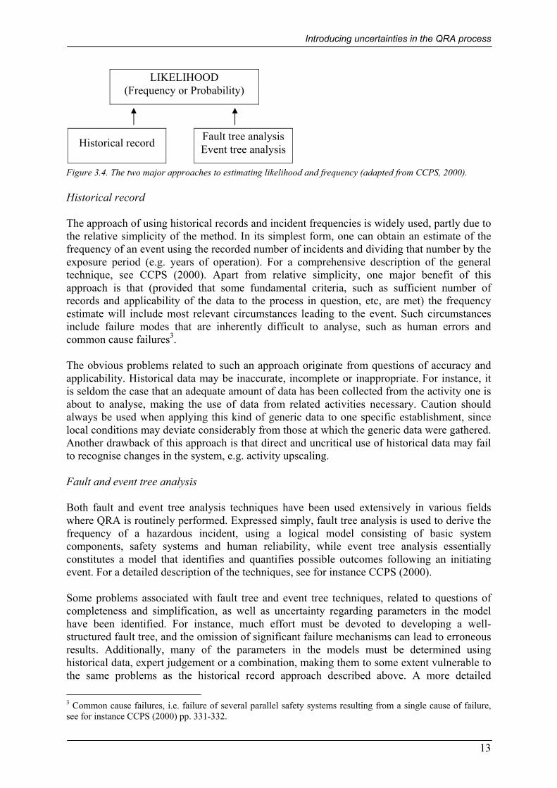
Figure 3.4. The two major approaches to estimating likelihood and frequency (adapted from CCPS, 2000). Historical record The approach of using historical records and incident frequencies is widely used, partly due to the relative simplicity of the method. In its simplest form, one can obtain an estimate of the frequency of an event using the recorded number of incidents and dividing that number by the exposure period (e.g. years of operation). For a comprehensive description of the general technique, see CCPS (2000). Apart from relative simplicity, one major benefit of this approach is that (provided that some fundamental criteria, such as sufficient number of records and applicability of the data to the process in question, etc, are met) the frequency estimate will include most relevant circumstances leading to the event. Such circumstances include failure modes that are inherently difficult to analyse, such as human errors and common cause failures3. The obvious problems related to such an approach originate from questions of accuracy and applicability. Historical data may be inaccurate, incomplete or inappropriate. For instance, it is seldom the case that an adequate amount of data has been collected from the activity one is about to analyse, making the use of data from related activities necessary. Caution should always be used when applying this kind of generic data to one specific establishment, since local conditions may deviate considerably from those at which the generic data were gathered. Another drawback of this approach is that direct and uncritical use of historical data may fail to recognise changes in the system, e.g. activity upscaling. Fault and event tree analysis Both fault and event tree analysis techniques have been used extensively in various fields where QRA is routinely performed. Expressed simply, fault tree analysis is used to derive the frequency of a hazardous incident, using a logical model consisting of basic system components, safety systems and human reliability, while event tree analysis essentially constitutes a model that identifies and quantifies possible outcomes following an initiating event. For a detailed description of the techniques, see for instance CCPS (2000). Some problems associated with fault tree and event tree techniques, related to questions of completeness and simplification, as well as uncertainty regarding parameters in the model have been identified. For instance, much effort must be devoted to developing a well-structured fault tree, and the omission of significant failure mechanisms can lead to erroneous results. Additionally, many of the parameters in the models must be determined using historical data, expert judgement or a combination, making them to some extent vulnerable to the same problems as the historical record approach described above. A more detailed 3 Common cause failures, i.e. failure of several parallel safety systems resulting from a single cause of failure, see for instance CCPS (2000) pp. 331-332.
LIKELIHOOD (Frequency or Probability)
Historical record Fault tree analysis Event tree analysis

Uncertainty in Quantitative Risk Analysis – Characterisation and Methods of Treatment
14
discussion of the methods used and pitfalls encountered when using expert judgement in risk analysis is presented in Chapter 5. 3.2.3 Consequence estimation The consequence estimation part of the analysis consists of several interacting parts. Physical models are used to estimate, for instance, concentrations of dispersed hazardous substances (at various locations around the source), shock wave overpressure from explosions, and the radiant flux from pool fires, jet fires, etc. Various effect models are used to predict the effect that the different outcome cases generated using the physical models mentioned above have on the object of the study, e.g. death or injury to human beings, effects on physical property such as damage to structures etc. Not surprisingly, all these exercises are, to some extent, afflicted with uncertainties, both stochastic and epistemic. Some general examples are given below. The actual physical modelling is a process in which mathematical models are used to represent reality, e.g. real physical processes, for example vapour dispersion. Obviously, any mathematical model of such a complex physical process can only be an approximation of that process, often with severe limitations on applicability. This kind of (knowledge-based) uncertainty is often difficult to quantify, although attempts have been made to establish uncertainty bounds on model estimates using a semi-quantitative approach (COWI, 1996a-d). This approach, together with a more thorough discussion on model uncertainty and means of reducing it, e.g. model validation exercises, will be further examined in Chapter 4. When modelling the effects on humans of exposure to toxic substances etc., the prevailing approach is to use results from dose-response tests performed on laboratory animals, by extrapolating these data to humans. “Most toxicological considerations are based on the dose-response function. A fixed dose is administered to a group of test organisms and, depending on the outcome, the dose is either increased until a noticeable effect is obtained, or decreased until no effect is obtained,” (CCPS 2000). It is not difficult to realise that such an approach will be associated with substantial uncertainties, both in the extrapolation from animal data to humans (knowledge-based uncertainty), and the fact that in any population exposed to the same dose of a substance there will be a significant spread in response (stochastic uncertainty). In addition, in order to make calculations less cumbersome, it is customary to use so-called probit4 functions to convert the dose response curve into a straight line, introducing yet another kind of model uncertainty. Both in the modelling of physical phenomena, such as vapour dispersion, and in the modelling of effects, the parameter values used in the models will be subject to both natural variability (e.g. wind speed) and epistemic uncertainty (e.g. constants for use in probit relationships differ from one study to another).
4 “For single exposures, the probit (probability unit) method provides a transformation method to convert the dose-response curve into a straight line.” (CCPS, 2000).

Introducing uncertainties in the QRA process
15
3.2.4 Estimation of risk The final step in the quantitative risk analysis process is to generate the actual risk measure. This is usually done by combining the probability of a certain outcome with the consequence of that particular outcome, then aggregating the information from all the outcomes identified. Numerous risk measures have been suggested in the literature, but here only two main groups of measures will be briefly introduced, i.e. individual risk measures and societal risk measures. For an exhaustive survey of various quantitative risk measures, see for instance, CCPS (2000). The term individual risk refers to the risk to which a person present at a specific location in the vicinity of a hazard is exposed. Individual risk is often expressed as the probability of fatality at that location per year. Several definitions of individual risk measures are in use, the most common being individual risk contours, which show the geographical distribution of individual risk, see Figure 3.5. For a comprehensive description of the methods used for calculating individual risk, together with a survey of definitions of individual risk measures, see CCPS (2000).
Figure 3.5. Example of an individual risk contour plot. Note: the contours connect points of equal individual risk of fatality, per year, (from CCPS, 2000). Societal risk is a measure of the risk to a group of people, and is often used to complement individual risk measures in order to account for the fact that major incidents often have the potential to affect many people. The most common form of presentation of societal risk is the FN-curve, which is the frequency distribution of multiple casualty events identified at the object under study, see Figure 3.6.

Uncertainty in Quantitative Risk Analysis – Characterisation and Methods of Treatment
16
Figure 3.6. Example of an F-N curve used to present societal risk. (Frequency of incidents resulting in N or more fatalities per year, from CCPS, 2000.) In order to be able to calculate the societal risk, the same information regarding frequencies and consequences of events as for the individual risk is needed. In addition, the calculation of societal risk requires a definition of the population at risk in the vicinity of the establishment. For a comprehensive description of the methods used for calculating societal risk, see CCPS (2000). The uncertainties introduced during this stage of the QRA process are principally related to assumptions and simplifications made in order to decrease the complexity of the analysis, i.e. the computational burden. Various symmetry assumptions regarding, for instance, equally probable wind directions, distribution of ignition sources and population distribution, together with assumptions on a single or a few wind and stability conditions, raise questions regarding the completeness of the analysis.
3.3 Methods of representing uncertainty In this section a brief introduction is given to different ways of representing uncertainty regarding variables and parameters used in risk modelling. 3.3.1 The probabilistic approach The, by far, most common approach used to represent uncertainty regarding a quantity, either stochastic or epistemic, is to use probabilistic distributions. As mentioned earlier in this chapter, there are two fundamental interpretations of the concept of probability, the frequentist and the Bayesian, where the frequentist school defines probability as a limiting frequency and the Bayesian school of thought defines probability as a degree of belief. Due to the high degree of epistemic, or knowledge-based, uncertainty involved in the QRA process the frequentist interpretation of probability, which is valid only if it is possible to identify a sample of independent, identically distributed observations of the phenomenon of interest, does not work in all situations making a Bayesian approach necessary.

Introducing uncertainties in the QRA process
17
Within a Bayesian framework probability distributions for unknown or varying quantities can be constructed using both “hard” data and subjective judgement. The resulting probability distribution is a representation of the assessor’s degree of belief regarding the probability of the assessed quantity to take a certain value, see Figure 3.7. A description of methods of eliciting information regarding unknown quantities from experts and transforming into probability distributions is given in Chapter 5.
CDF for A
0
1
0 5 10a
P(A
≤ a
)
Figure 3.7. Probability distributions are often used to represent uncertainty regarding a quantity. The quantity A is assumed to be normally distributed with mean = 5 and standard deviation = 1. Here, the distribution for A is presented as the Cumulative Distribution Function (cdf). 3.3.2 Interval representation The interval representation of uncertainty is useful in situations where we are absolutely sure about the bounds of a quantity, but we know little or nothing else. Here is a simple example5. A golfer makes two birdies over the first three holes. How many birdies will he make in total over the whole round of 18 holes? Unless we have no other information about the situation than that given above, a reasonable way of expressing our uncertainty about the situation without having to make any (unjustified) assumptions would be to give our answer in the form of an interval between 2 and 17 (the total range of possible birdies over the 18 holes). Interval analysis can be used to estimate the possible bounds on model outputs using bounds (i.e. intervals) to represent uncertainty about model inputs and parameters. 3.3.3 The probability bounds approach The uncertainty in a scalar number may be described as an interval as stated above. In the same way, a pair of probability bounds may be used to circumscribe the uncertainty regarding a probability distribution (Ferson et al., 1996, 1998, 1999). Probability bounds may be constructed from parametric probability distributions where the parameters are uncertain, as shown in Figure 3.8, where parameter X is a log-normal distribution with the mean µ = [2.5,3] and standard deviation σ = [0.8,1]. It is also possible to construct probability bounds in a
5 Example given by J. Arlin Cooper, Sandia National Labs (USA), at the workshop “Beyond Point Estimates – Risk Assessment Using Interval, Fuzzy and Probabilistic Arithmetic”, organised by the Society for Risk Analysis, 5 December 1999.

Uncertainty in Quantitative Risk Analysis – Characterisation and Methods of Treatment
18
distribution-free context where the particular shape of the distribution cannot be specified. In these cases bounds on the possible distributions that are consistent with the empirical information are generated. For example, the only information available on parameter Y is its min = 2, max = 3 and mean = 2.4. Nothing is known about the shape of the distribution. In Figure 3.8, the bounds on all possible distributions given this information are shown for parameter Y. Probability bounds have been derived for various sets of information regarding the uncertain variable. Examples of such sets of information are sample data, knowledge about the mean and variance, knowledge about the minimum, maximum and mode etc. (Ferson et al. 1999).
X
0
0.2
0.4
0.6
0.8
1
0 2 4 6 8
x
P(X)
< x
Y
0
0.2
0.4
0.6
0.8
1
1.5 2 2.5 3 3.5
y
P(Y)
< y
Figure 3.8. Examples of probability bounds representing uncertainties in unknown quantities X and Y. See Section 7.5 for examples of arithmetic operations on probability bounds. For a mathematical background on how to generate the probability bounds, see Ferson et al. (1996, 1999). 3.3.4 Fuzzy representation The theory of fuzzy sets was introduced by Zadeh (1965), with the original objective of providing a mean of modelling the uncertainty (or vagueness) of natural language. Within this framework, notions like “densely populated” and “relatively strong winds” can be formalised using so-called membership functions. The main idea is easily grasped by a comparison with classical set theory. As stated by Isukapalli (1999): In classical set theory, the truth value of a statement can be given by the membership function µA(x), as:
( )
∉∈
=AxAx
xA iff0iff1
µ (3.1)
On the other hand, fuzzy theory allows for a continuous value of µA between 0 and 1, as
( )
<<∉∈
=. tobelongspartially if10;
iff0iff1
AxppAxAx
xAµ (3.2)
Fuzzy arithmetic, which is an offshoot from fuzzy set theory, and can also be regarded as a generalisation of interval analysis, will be briefly introduced in Section 7.6.
Introducing uncertainties in the QRA process
19
3.4 Background studies on methods of considering other types of uncertainty 3.4.1 General quality uncertainty In (COWI, 1996a-d) an interesting method of incorporating (quantitatively) uncertainty related to general quality issues, such as science and engineering state of the art, improper definition of the assessment problem, competence of the analyst team etc. The scope of this method is very broad and perhaps unattainable at a practical level, but still it provides an interesting platform for further discussions regarding these matters. A brief description of the methodology is presented in Appendix 2. 3.4.2 Management and organisational safety The concept of incorporating organisational factors and effects of managerial decisions into the results of a risk analysis has gained increased interest in recent years. Hale & Hovden (1998) presents “a review of approaches to organisational aspects of safety, health and environment”, where several research projects in this area are identified and presented. In this section, two examples of recent projects, I-risk and SAM, are briefly introduced. For a comprehensive survey of a number of similar projects, see Sklet et al. (1999). I-risk is a European project involving partners from the UK, Greece, the Netherlands and Norway. The overall objective of the project is to provide a method making it possible to integrate the technical model of an installation with a safety management model of an organization (Hale et al., 1998a). Another attempt to capture and model human behaviour and management effects in risk analysis has been presented by Murphy & Paté-Cornell (1996). The SAM (System-Action-Management) framework provides a general approach for addressing the human and management causes of system failure. The approach is based on the assumption that most accidents in complex technical systems are not caused by pure technical problems, or isolated human errors, which is the perhaps most common approach to causal analysis today. Instead the failure of a system is regarded as a consequence of management and organisational factors that influence the decisions and actions of individuals. The SAM framework is a three level approach, which involves the physical system level, where a probabilistic risk analysis model is used. At the intermediate level, human decisions and actions that affect system performance is addressed, and at the highest level, the management and organisational factors that influence decisions and actions are included. The SAM framework, including examples of applications, is presented in, for instance, (Murphy & Paté-Cornell, 1996), and in (Paté-Cornell, 1998).

Uncertainty in Quantitative Risk Analysis – Characterisation and Methods of Treatment
20
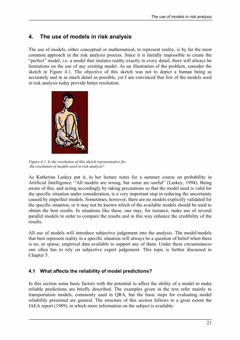
The use of models in risk analysis
21
4. The use of models in risk analysis The use of models, either conceptual or mathematical, to represent reality, is by far the most common approach in the risk analysis process. Since it is literally impossible to create the “perfect” model, i.e. a model that imitates reality exactly in every detail, there will always be limitations on the use of any existing model. As an illustration of the problem, consider the sketch in Figure 4.1. The objective of this sketch was not to depict a human being as accurately and in as much detail as possible, yet I am convinced that few of the models used in risk analysis today provide better resolution.
Figure 4.1. Is the resolution of this sketch representative for the resolution of models used in risk analysis? As Katherine Laskey put it, in her lecture notes for a summer course on probability in Artificial Intelligence: “All models are wrong, but some are useful” (Laskey, 1994). Being aware of this, and acting accordingly by taking precautions so that the model used is valid for the specific situation under consideration, is a very important step in reducing the uncertainty caused by imperfect models. Sometimes, however, there are no models explicitly validated for the specific situation, or it may not be known which of the available models should be used to obtain the best results. In situations like these, one may, for instance, make use of several parallel models in order to compare the results and in this way enhance the credibility of the results. All use of models will introduce subjective judgement into the analysis. The model/models that best represent reality in a specific situation will always be a question of belief when there is no, or sparse, empirical data available to support any of them. Under these circumstances one often has to rely on subjective expert judgement. This topic is further discussed in Chapter 5.
4.1 What affects the reliability of model predictions? In this section some basic factors with the potential to affect the ability of a model to make reliable predictions are briefly described. The examples given in the text refer mainly to transportation models, commonly used in QRA, but the basic steps for evaluating model reliability presented are general. The structure of this section follows to a great extent the IAEA report (1989), in which more information on the subject is available.

Uncertainty in Quantitative Risk Analysis – Characterisation and Methods of Treatment
22
Figure 4.2. The five classes affecting the reliability of model predictions (adapted from IAEA, 1989). 4.1.1 Problem specification Obvious at it might seem, one should not underestimate the importance of a thorough specification of the scenario or problem that the model is intended to address. Important factors to focus on when evaluating the reliability of models in this sense are, for example, the intended use of the results and the temporal/spatial resolution required. Failure to accurately define the scenario or problem in question might lead to the classical mishap of having a model that produces correct results for the wrong problem. It might well be that the difference between the model predictions and the observed reality is completely dependent on an inadequate specification of the characteristics and important mechanisms controlling the scenario. 4.1.2 Conceptual and computational model formulation A conceptual model is useful and necessary because it is needed to identify, for example, processes, pathways, compartments and interactions between compartments, processes and mechanisms that are to be considered explicitly while evaluating a scenario. Naturally, for practical reasons, such as limited or low-quality data, it is virtually impossible to include all imaginable processes and mechanisms in the conceptual model. As always, it will, to some extent, be a matter of judgement whether a chosen conceptual model is suitable for a specific scenario. The computational model, i.e. the model that is actually used for computations in risk analyses, is simply the set of equations and parameters used to obtain quantitative results. Various forms of quality assurance procedures, such as model verification and model comparison, are available and necessary for testing computational models. Basically, verification of the computational model implies testing the model against a known solution to identify any errors in the set of equations, numerical solutions, etc. Obviously, as stated in (IAEA, 1989), the extent of verification will depend on the intended use of the model. 4.1.3 Estimation of parameter values Regardless of how sophisticated a model one has access to for evaluating a specific scenario, the accuracy of the results will be dependent to a high degree on the constants and independent variables of the equations in the model. Undoubtedly the ideal situation would be
Specification of the problem (scenario)
Formulation of the conceptual model
Estimation of parameter values
Calculation and documentation of results
Formulation of the computational model

The use of models in risk analysis
23
to have access to experimental data pertinent to the specific scenario or situation one wishes to evaluate. However, this is seldom the case and model parameters often have large uncertainties associated with them. Often one has to rely on somewhat subjective expert judgements of estimates of model parameters. One basic prerequisite regarding the computational model one intends to use in an analysis is to ensure that the values the parameters may take lie within the range that the model can handle. For example, if a certain dispersion model is only valid for wind speeds between 2 and 8 m/s, and the typical wind speeds in the area one is about to analyse range up to 15 m/s, one would have to look for another model that can handle such a range. For a comprehensive discussion regarding ranges of valid parameter values in some widely used dispersion and transportation models, see for instance COWI (1996c). Methods of parameter uncertainty analysis will be extensively described in Chapter 7. 4.1.4 Calculation, presentation and documentation of results “Among the more obvious factors affecting the reliability of model predictions are those associated with the calculation and documentation of results”, (IAEA, 1989). This source of uncertainty and potential source of error will not be discussed at length here, however, it may be pointed out that there are quality assurance procedures available to minimise these problems, e.g. benchmark studies and peer review procedures.
4.2 Treatment of model uncertainty Whereas the intention in Section 4.1 was to provide a general discussion on what might affect model reliability, this section will briefly describe some approaches to dealing with model uncertainty explicitly. A short discussion concerning model validation, a topic with an immense body of literature available for the interested reader, will be followed by some approaches to handling model uncertainty in the practical situation. 4.2.1 Model validation The importance of using models that have been proven valid for the specific problem under consideration is self-evident. Model validation in this context generally refers to exercises where model predictions are tested against experimental data that are independent of the data set used to develop the model. The topic of model validation has been extensively discussed in many areas. One example related to QRA activities is the European initiative on “Harmonisation within Atmospheric Dispersion Modelling for Regulatory Purposes”, which was launched in 1991 to promote increased cooperation and standardisation of atmospheric dispersion models for regulatory purposes (Olesen, 2001). Since then several conferences and workshops have been held resulting in, among other things, a Model Validation Kit, which is a collection of three experimental data sets accompanied by software for dispersion model evaluation. Extensive and detailed information on this initiative can be found at, for instance, www.dmu.dk/AtmosphericEnvironment/harmoni.htm (2002-02-05). Similar efforts have been made in other areas. A general rule is that whenever a risk analyst is about to use a model it is up to that analyst to assess the usefulness of the model in the specific situation. Situations might arise, however, where model validation is not viable, making model comparison studies, possibly by using

Uncertainty in Quantitative Risk Analysis – Characterisation and Methods of Treatment
24
theoretical test cases, one way to evaluate model predictions. However, model comparison exercises can not by any means replace a proper validation process, since each of the models used in the exercise might contain inaccuracies. For more information on methods of evaluating model reliability, see for instance COWI (1996c) or the report of the Model Evaluation Group (1994). For a practical example of a model evaluation exercise, see Hanna et al. (1991). 4.2.2 Treatment of model uncertainty in the practical situation As pointed out in Section 3.1, model uncertainty is one of the major sources of uncertainty when performing a QRA. Nevertheless, relatively modest attention is generally directed explicitly towards this kind of uncertainty, compared, for instance, with parameter uncertainty. For example, in the survey by Abrahamsson (to be published), in which some twenty risk analysis reports where studied, none of them explicitly discussed the possible impact of model uncertainty on the results. In most of the analyses different models were used with no comment on their applicability to the specific situation, and in some of them the problem was “dealt with” by simply stating that the models are “not perfect representations of reality”. It is not possible to devise general rules on how to deal with model uncertainty that will satisfy every situation. Sometimes a qualitative discussion may suffice, while other situations may call for more sophisticated treatment. Apart from model evaluation exercises, it is possible to outline three major approaches to the practical treatment of model uncertainty in risk analysis. Firstly, in the Dutch guidelines for QRA (Committee for the Prevention of Disasters, 1999) discussed earlier, the main approach is to prescribe which models to use in the different stages of an analysis, an approach that has obvious advantages regarding comparability between analyses and consistent decision making. To some extent, such a prescriptive method indicates that the individual or organisation responsible for of the Guidelines accepts responsibility for any inaccuracies introduced into the analysis by imperfect models. A conceptually different approach would be to try to quantify the uncertainty ascribed to a specific model, for instance, by introducing a knowledge uncertainty parameter into the model representing one’s belief in the “correctness” of the model predictions for the specific situation. This model uncertainty parameter could then be treated in the same way as other uncertain parameters in the model (see Chapter 7 for a thorough review of methods of parameter uncertainty analysis). The process of establishing the (knowledge-based) model uncertainty parameter one would, by definition, have to include the subjective judgement of the analyst, something that calls for a structured methodology. One interesting approach to establishing bounds on the model uncertainty parameter is presented in COWI (1996a), previously introduced in Section 3.4, where the model uncertainty class is decomposed into three sub-classes which are assessed separately and then aggregated to form one uncertainty factor representing the total model uncertainty. The three sub-classes of model uncertainty are (COWI, 1996a):
1. relevance, i.e. to what extent the model used covers the specific situation 2. validity, i.e. how well the model has been validated 3. the natural variability of the modelled phenomenon.

The use of models in risk analysis
25
Based on these three “sub-classes” a semi-quantitative assessment is performed using tables provided in the guidelines. In Table 4.1 the guidance given for the model uncertainty factor UF3 is presented: Table 4.1. Sub-classes of the model uncertainty factor UF3 (adapted from COWI, 1996a). Small uncertainty
1 < UF3 < 2 Moderate uncertainty 2 < UF3 < 10
Large uncertainty 10 < UF3
Relevance Validity Variability
High High Low
Medium Medium Medium
Low Low High
The total model uncertainty factor is then calculated using:
( )2/1
1
2lnexp
= ∑=
n
iiUFUF (4.1)
The perhaps most appealing feature of such an approach is that it forces the analyst to explicitly consider model uncertainty in the analysis (in addition to the quantification of the uncertainty factor, a qualitative description of the three sub-classes is required in the guidelines.) The obvious drawback of the quantification exercise is that it tends to be somewhat arbitrary. Finally, a fairly common approach is to make use of several parallel models in order to enhance credibility in the results. An appealing feature of this methodology is that it is possible to compute bounds on the results which will enclose all possible results from the models used, and these bounds can be used further in the analysis. The obvious pitfall of using parallel models is that they might be based on the same fundamental mechanisms, the same (possibly erroneous) data set or that they share the same biases. The fact that several different models produce more or less the same results is no guarantee that they are indeed accurate.

Uncertainty in Quantitative Risk Analysis – Characterisation and Methods of Treatment
26

The use of expert judgement in risk analysis
27
5. The use of expert judgement in risk analysis
5.1 General discussion As mentioned in previous chapters, the use of expert judgement becomes necessary when one does not have a complete understanding of the underlying fundamental mechanisms. This may involve the structure of the models used as well as uncertainty regarding the quantification of the variables involved. The task of eliciting useful information based on various experts’ subjective opinions “is not to be taken lightly”. There is no universal method that applies to all situations regarding this matter. In fact, there is not one “scientifically correct” method at all (Paté-Cornell 1996). Nevertheless, several structured methods of eliciting information from experts have been suggested in the literature and proven useful in practical risk analyses. For practical examples see, for instance, Morgan & Henrion (1990). In this chapter some basic methods of eliciting and aggregating information from experts will be briefly introduced followed by a discussion on the psychology of judgement under uncertainty and a presentation of the basic requirements of elicitation exercises. This discussion is solely aimed at representing uncertainty in the unknown variable by using probabilistic measures such as probability distributions, since that is by far the most common approach in risk analysis today.
5.2 Elicitation In this section some general approaches to assessing probabilities for specific values of unknown variables will be briefly introduced. Somewhat simplified, such assessments can be divided into two categories, i.e. the assessment of discrete probabilities and the assessment of continuous probabilities. 5.2.1 Encoding discrete probabilities The encoding of discrete probabilities, i.e. the probability of a discrete quantity (e.g. events) can be done in several different ways, the simplest being to directly ask the interviewee (expert), “What is your belief regarding the probability that event A will occur?” It is, however, likely that the interviewee will find it difficult to answer such direct questions, let alone place any confidence in the answer (Clemen, 1996).

Uncertainty in Quantitative Risk Analysis – Characterisation and Methods of Treatment
28
The perhaps most common approach is based on a thought experiment where the expert is asked to compare (and choose between) two lottery-like games, which can both result in a prize (X or Y) where prize X is strongly preferred to prize Y (e.g. price X is a free trip around the world and prize Y is a t-shirt.) For example: The interviewee is asked to compare the lottery: Win prize X if event A6 occurs Win prize Y if event A does not occur With the lottery: Win prize X with known probability p. Win prize Y with probability 1 – p. The second lottery is called the reference lottery. It is of major importance that the probability mechanism for the reference lottery is well defined and easy for the interviewee to understand. Classical mechanisms often used are drawing coloured balls from an urn in which the proportion of coloured balls is known to be p, and the “probability wheel” with a known area representing “win prize X”. When spun, if the pointer lands on the “win prize X” area the interviewee wins prize X, see Figure 5.1.
The probability wheel
Figure 5.1. The probability wheel. In this example the ”win prize X” area is the striped area giving a probability p = 0.35. The trick here is to adjust the probability p of winning prize X in the reference lottery until the interviewee is indifferent (has no preference) between the two lotteries. Then the subjective probability assessed by the interviewee for event A is p. When a series of probability assessments has been performed one must check the probabilities obtained for consistency, i.e. the probabilities assessed by the interviewee obey the laws of probability theory. 5.2.2 Encoding continuous probabilities The classical approach to encoding continuous probabilities is to apply the technique for encoding discrete probabilities to assess several cumulative probabilities and then plot these in a diagram making a rough CDF (cumulative distribution function). Consider the following example.
6 Event A may be that it will rain in Lund a certain day, for example.

The use of expert judgement in risk analysis
29
We want the interviewee to express his/her beliefs regarding the snow depth at a certain place in the Swedish mountains next New Year’s Eve, using a probability distribution to represent his/her uncertainty. The characteristic question would be to assess P(snow depth ≤ a) where a is a certain value. One assessment point could for instance be P(snow depth ≤ 50 cm), where the outcome “snow depth ≤ 50 cm” is a discrete outcome that can be assessed using, for instance, the reference lottery approach described above. To be able to construct a CDF in this manner, the cumulative probability would have to be assessed for a number of points. Suppose the following assessments were made: P(snow depth ≤ 5 cm) = 0.00
P(snow depth ≤ 25 cm) = 0.05 P(snow depth ≤ 50 cm) = 0.25 P(snow depth ≤ 75 cm) = 0.60 P(snow depth ≤ 100 cm) = 0.80 P(snow depth ≤ 150 cm) = 1.00 In Figure 5.2 these cumulative probabilities are plotted as a rough CDF representing the interviewee’s beliefs (uncertainty) about the unknown quantity:
CDF for snow depth
0
0.5
1
0 50 100 150x [cm]
P(sn
ow d
epth
≤ x
)
Figure 5.2. CDF representing the interviewee’s beliefs about the snow depth at a certain place in the Swedish mountains next New Years’ Eve. The methodology used in the example above is usually referred to as a “fixed value” method. An alternative strategy to construct the CDF above would be to do the reverse, i.e. by choosing some fractiles on the vertical axis and assessing the corresponding values of the snow depth (the “fixed probability” method). For a comprehensive discussion on these and more techniques for encoding probabilities and discussions on experiments related to the merits of each of them, see for example Cooke (1991) or Morgan & Henrion (1990).
Uncertainty in Quantitative Risk Analysis – Characterisation and Methods of Treatment
30
5.2.3 Basic structure of the assessment protocol Generally, an elicitation exercise follows some kind of protocol, i.e. a documented structure for the elicitation process. There is no single procedure available that will guarantee “success” in any given situation, indeed several different protocols have been used in practise (see, for example, Morgan & Henrion (1990)). Nevertheless, a (simplified) presentation of the basic requirements in elicitation exercises as given by Clemen (1996) is given below. According to Clemen at least the following steps should be included in the assessment protocol.
• Background, i.e. thorough identification and description of the variables for which expert assessment is needed. It may be possible to assess some variables using conventional scientific studies while others may require expert assessment.
• Identification and recruitment of experts, possibly with help from professional associations.
• Motivating experts. Some scientists might be reluctant to participate in such exercises since they feel that their opinions might not be “correct” in a scientific sense. However, since variables that require expert assessment cannot be assessed using traditional, scientific methods and decisions still have to be made using the best information available, there is no realistic alternative.
• Structuring and decomposition, i.e. exploring the experts’ understanding of the causal and statistical relationships between the assessed variables. For instance, the probability distribution of one variable may need to be assessed conditional on other variables.
• Probability assessment training, e.g. explanation of the basic principles of the assessment and of known heuristics and biases related to such exercises (see Section 5.3.)
• Probability elicitation and verification, i.e. the actual assessment of the unknown variables made by the expert, always under the guidance of an individual trained in the elicitation process.
• Aggregation of different experts’ probability distributions, see Section 5.4. For more information on this subject, see Clemen (1996) and “Attributes of a Good Assessment Protocol” described in Morgan & Henrion (1990).
5.3 Heuristics and biases Inherent in the concept of using expert judgement in risk assessment is that we are dealing with unknown quantities of some kind, for which we have no or limited hard data. In situations where people are asked to estimate probabilities or degrees of belief for such quantities they tend to use various rules of thumb, or heuristics, in their assessments. In some situations however, such heuristics may lead to predictable “errors”, where “error” should be interpreted as an estimate that is not in accord with the subject’s “true” beliefs. Heuristics that lead to errors as described above are referred to as biases, i.e. in this context biases are related to “misperceptions” of probabilities. Whenever one intends to use experts (or any human being, whether they want to call themselves experts or not…) for the estimation of unknown quantities, one should be aware of the possible pitfalls these biases might constitute. In this section some recognised heuristics that might lead to errors such as those described above will be briefly introduced. For a more exhaustive presentation of this topic see, for example, Kahneman, Slovic and Tversky (1982) or Cooke (1991). The information and examples in the

The use of expert judgement in risk analysis
31
following five sub-sections are, to a great extent, based on Cooke (1991), one of the standard references in the field of expert judgement. 5.3.1 Availability The concept of availability concerns the phenomenon that when asked to estimate the size of a “class” (e.g. the number of deaths due to residential fires in a year) people tend to base their estimates upon the ease with which such instances can be recalled. The availability heuristic has proved to have considerable impact on people’s perception of different risks. In a study by Slovic, Fischoff and Lichtenstein (1982) a large number of lay people were asked to estimate the probability of death from various causes. The typical response pattern was that the risks from well-publicised causes of death (e.g. botulism and tornadoes) were strongly overestimated, whereas the risks of “unglamorous” causes (e.g. heart disease and stomach cancer) were underestimated. Figure 5.3 shows the typical response pattern in the study.
Figure 5.3. Relationship between judged frequency and the actual number of deaths per year for 41 causes of death. If judged and actual frequencies were equal, the data would fall on the straight line. The points, and the curved line fitted to them, represent the average response of a large number of lay people. As an index of the variability across individuals, vertical bars are drawn to depict the 25th and 75th percentiles of the judgements for botulism, diabetes and all accidents. The range of responses for the other 37 causes was similar (from Slovic, Fischoff and Lichtenstein, 1982). 5.3.2 Anchoring A known phenomenon when people are asked to estimate the value of an unknown quantity is that they tend to fix on an initial value and then adjust this value. This phenomenon is called anchoring, and the problem with this heuristic is that frequently the adjustment that people make is insufficient. In an experiment by Tversky and Kahneman (1982a) subjects were asked to estimate what percentage of the member nations in the UN were African. A number between 1 and 100 was generated by spinning a wheel (in the subject’s presence). The median estimate of the percentage of African countries was 25 for a group with “anchor” number 10, and 45 for a group with “anchor” number 65.

Uncertainty in Quantitative Risk Analysis – Characterisation and Methods of Treatment
32
A perhaps more relevant instance of anchoring to expert judgement (or elicitation of expert estimations) occurs when subjects are asked to estimate the fractiles7 of a continuously distributed variable. When subjects are asked to estimate for instance the 5% and 95% fractiles of a distribution, they appear to fix on a central value of the distribution and then adjust to obtain the fractiles of interest. The 5% and 95% fractiles obtained in this way are often too close to the central value, i.e. the true value will too often fall outside the given interval. 5.3.3 Representativeness Representativeness is a phenomenon related to conditional probabilities. In short, the representativeness heuristic has important implications (in terms of biases) when a subject is asked to estimate the conditional probability p(A|B) that event A will occur given that event B has occurred. Experiments have shown that when making such judgements, subjects tend to rely on an assessment of the degree of similarity of events A and B (Cooke, 1991; Tversky and Kahneman, 1982b). In addition, the representativeness heuristic leads people to ignore effects due to sample size. An experiment by Tversky and Kahneman (1982c) illustrates this effect.
A certain town is served by two hospitals. In the larger hospital about 45 babies are born each day, and in the smaller hospital about 15 babies are born each day. As you know, about 50% of all babies are boys. However, the exact percentage varies from day to day. Sometimes it may be higher than 50%, sometimes lower. For a period of 1 year, each hospital recorded the days on which more than 60% of the babies born were boys. Which hospital do you think recorded more such days?
Of the 95 subjects responding to this question, 21 opted for the larger hospital, 21 for the smaller hospital, and 53 thought that both hospitals recorded about the same number of such days. Of course, the smaller hospital is much more likely to see more than 60% boys on any given day. 5.3.4 Control One possible source of distorted probability assessments is that subjects tend to act as if they have some sort of control over situations that they could not possibly have any influence over. One example given by Cooke (1991) is an experiment carried out on office workers in New York. One group of 26 subjects was given the opportunity to buy a ticket for an office lottery at $1 each. The prize of $50 would go to the winning ticket, to be drawn from an urn. The subjects were allowed to choose their own ticket. A second group of 27 subjects was given the opportunity to buy tickets for the same lottery but were simply given tickets and were not allowed to choose. Each subject was then approached by the experimenter and asked:
Someone in the other office wants to get into the lottery, but since I’m not selling tickets any more, he asked me if I’d find how much you’d sell your ticket for. It makes no difference to me, but how much should I tell him?
7 The k% fractile of a continuously distributed quantity X is the smallest value xk such that p(X≤xk) ≥ k/100.
The use of expert judgement in risk analysis
33
In the group that chose their own ticket, the median resale price was $8.67, whereas in the group that was given their tickets, the median resale price was $1.96. 5.3.5 Overconfidence and calibration In Cooke (1991) a rough definition of calibration regarding expert judgement is given: “A subjective assessor is well-calibrated if for every probability value r, in the class of all events to which the assessor assigns a subjective probability value r, the relative frequency of occurrence is equal to r. Calibration represents a form of empirical control on subjective probability assessments”. Whether an expert (or a person who is asked to estimate some quantity) is well calibrated or not can be measured in two different types of test: discrete tests and quantile or fractile tests. For discrete tests, see Cooke (1991). When one is interested in someone’s assessment of a variable with a continuous range one can use fractile tests for calibration. For example, one may be interested in the maximal capacity (measured, for instance, in people/min) of a particular escape route in a building under certain conditions. It is not likely that anyone would predict this value with any certainty (not without making unjustified assumptions anyway), but it would be possible for an expert to give a subjective probability distribution representing the uncertainty in the estimate (see Section 5.2.2). Using the following type of question enables us to learn about this subjective probability distribution: “For which x is your probability 25% that the capacity of the escape route is less than or equal to x?” The answer will be called the subject’s 25% fractile. In the same manner, a whole set of fractiles can be elicited to obtain a representation of the subject’s subjective probability distribution for the unknown variable. The matter of calibration regarding fractile tests can be expressed as follows: “Suppose we ask an expert for his 1%, 25%, 50%, 75% and 99% fractiles for a large number of variables, for which the actual values later become known. If the expert is well calibrated, then we would expect that approximately 1% of the true values fall beneath the 1% fractiles of their respective distributions, roughly 24% should fall between the 1% and the 25% fractiles, etc. The interquartile range is the interval between the 25% and the 75% fractiles. We would expect 50% of the true values to fall within the interquartile ranges.” (Cooke, 1991).
5.4 Different approaches to the aggregation of expert opinions Difficulties naturally arise when the experts disagree about the problem in question, for instance the likelihood estimates regarding initial events. There are many ways to circumvent this problem, some more appropriate than others. One’s first thought might be to just look for some kind of common value or range that is within, or at least in the vicinity of, everybody’s estimated confidence interval. This is clearly not the proper way to go about it, since experts tend to underestimate uncertainties. It could well be that the most well-informed expert has the largest uncertainty interval, and using this method would only lead to the choice of value or segment being decided by the narrowest uncertainty interval obtained. Paté-Cornell (1996) states: “The methods that are most likely to provide a reasonable degree of objectivity are those that focus on the construction of a set of hypotheses and on the assessment of axiomatically correct probability distributions based on all scientific evidence. This requires a process that starts with gathering all available data, then assessing and aggregating relevant probabilities in an orderly and logical fashion.” It is not difficult to see that doing this properly will be a time-consuming and expensive task.
Uncertainty in Quantitative Risk Analysis – Characterisation and Methods of Treatment
34
The three classical ways of aggregating expert opinions described in Paté-Cornell (1996) are: • The analytical approach, where each of the experts provides their probability distribution.
Then someone (e.g. the decision maker) creates a combined distribution, for example by equal weighting of the distributions provided by the experts, or by somehow assigning different weights to the different distributions provided.
• The iterative approach (e.g. the Delphi technique), where the different assessments
provided by the experts are averaged by the analyst, then sent back to the experts who are given the possibility to revise their opinion based on what the other experts have said. The process is repeated until the value converges, which is usually rather quickly, provided that there aren't one or more experts who think they know something the others don’t.
• The interactive approach, where the experts are asked to debate and explain their
assessments. The experts are given the chance to exchange information about the evidence base, on which they rely, which further helps the objectivity process.
For a survey of literature dealing with the problem of aggregating information from multiple experts with different opinions, see Morgan & Henrion (1990). It should be noted, however, that there might be situations in which aggregation of information provided by different experts is not desirable. For instance, one could argue that creating a combined distribution for the uncertainty quantity based on the different distributions provided by the experts will produce a result that nobody actually believes in. The common approach suggested by scientists advocating such a point of view is to make use of parallel distributions (models) for, or bounds on, the unknown quantity in the analysis. In this chapter some basic methods of eliciting information on unknown variables from experts in the form of probabilities have been discussed. Probabilistic measures are, however, not the only ones used to represent uncertainty (although they are by far the most common) about an unknown variable. In Chapter 7 some approaches to uncertainty propagation, such as interval analysis and fuzzy arithmetic are briefly introduced. The kind of information needed when using such measures of uncertainty is also discussed in Chapter 7.

The use of databases in risk analysis
35
6. The use of databases in risk analysis
6.1 General introduction Accident and other kinds of experience databases traditionally play a significant role in the risk analysis and risk management process. In this chapter a fairly general discussion on the merits of experience databases in risk analysis, mainly based on Davidsson et al. (1999), is presented. Depending on the characteristics of the hazards connected with a certain activity, it is possible to discern three major safety strategies (Rasmussen, 1994; 1997), see Figure 6.1.
Figure 6.1. Hazard source characteristics and risk management strategies, adapted from Rasmussen (1997). It is possible to relate the use of experience databases to the type of safety strategy implemented. In category 1, empirical safety strategy, which is often applied when dealing with a complex set of hazard sources with high frequencies of accidents but usually with potential for only relatively small consequences, experience databases are mainly used for statistical analysis, e.g. analysis of trends and as an aid in hazard identification. In category 2, evolutionary safety strategy, often applied in the process industry and transportation sector, the hazards are characterised by low accident frequencies but with the potential of substantial consequences. Quantitative risk analysis is a common tool in this domain. Within this category, experience databases are frequently used for identification of hazard sources and accident event sequences, for estimating the probability of failures and as support for consequence estimation. In category 3, analytical safety strategy, characterised by hazard sources with extremely low accident frequencies but with the potential of truly catastrophic consequences, e.g. nuclear power plant accidents, experience databases are frequently used as input for the analysis of initiating events and of the reliability of safety barriers.

Uncertainty in Quantitative Risk Analysis – Characterisation and Methods of Treatment
36
6.2 The use of databases in the different stages of an analysis In Section 3.2 the uncertainties introduced at different stages of a QRA were discussed. In this section a short presentation will be given of some ways in which experience databases can be of use in the different stages of such an analysis. The main problems in the identification phase of an analysis are related to questions of completeness, e.g. have all the relevant scenarios been identified? In this phase experience databases used together with a structured methodology for identification, such as HAZOP and FMEA procedures, will provide means of keeping completeness uncertainty to a minimum. Used wisely, experience (accident) databases have the potential to both increase direct knowledge about possible accident scenarios and to serve as input in the creative process of identification. For examples of existing databases for use in the identification phase, see Appendix 1. In the frequency estimation phase of an analysis experience databases can be used both to calculate the expected frequency directly from historical data, and to estimate the probabilities of parameters of logical models used for calculating frequencies of events, see Section 3.2. Obviously, such analysis places special requirements on the type of data included in the database. Besides identification and general descriptions of accidents or failures, the database must also contain information on relevant parameters that might affect the frequency of accidents, (e.g. the number of units/systems in operation, the total number of years in operation, the total number of accidents, etc.) For examples of existing databases for use in the frequency estimation phase, see Appendix 1. The consequence estimation part of an analysis is usually performed using theoretically and/or empirically established models of physical phenomena like vapour dispersion, and of effects on human beings. In situations where the possible outcomes of accidents are difficult to model, experience from previous accidents might prove useful in establishing probable estimates of the consequences. For such an approach to be successful, the information in the database must include detailed (objective) descriptions of the effects and damage caused by the accident and, if possible, the damage mechanism. Information about subsequent events might also prove helpful.
6.3 Requirements on databases to be used in risk analysis The requirements on databases to be used in risk analysis may vary considerably depending on several factors, such as the objective of the analysis or the stage of the analysis. In some stages of an analysis very specific, detailed information will prove necessary, while other stages require large, comprehensive experience databases. As a result, it might be difficult to find a database that covers all one’s needs simultaneously. However, some basic requirements are common for all use of experience databases in risk analysis (Davidsson et al., 1999):
The use of databases in risk analysis
37
• Accessibility • User-friendliness • Reliability (i.e. traceable data sources) • Relevance (e.g. with respect to the analysed object) • Coverage • Regular updating
A quantitative analysis of experience data is needed when performing QRA in order to calculate (estimate), for instance, failure frequencies, consequences and effects. When analysing data from a specific database it is of importance to know the criteria for registration in that database, i.e. why are the data there? If possible, it might also be of importance to know whether some data have been deliberately omitted from the database, e.g. accidents where the consequences are looked regarded negligible. Above all, the frequency analysis is greatly dependent on specific descriptions (calculations) of relevant parameters that might affect the frequency of accidents, e.g. the number of units/systems in operation, the total number of years of operation, the total number of accidents, etc. A fortunate fact, but still a fact that might pose some problems when it comes to estimating the frequency of events, is that large-scale accidents tend to occur rather seldom. As a result of this, a company often has limited hard data regarding large-scale accidents within its own organisation. This increases the need for more generic data, e.g. data that have been collected from a large number of facilities within the same principal sphere of activities. The problems related to more generic data are quite obvious. One must ensure that the relevance of the data used in an analysis is acceptable. For a more comprehensive discussion of the requirements of databases to be used in a risk analysis see, for instance, Davidsson et al. (1999). For an extensive list (and description) of existing databases, see Lees (1996). For a description of some major experience databases, see Appendix 1.

Uncertainty in Quantitative Risk Analysis – Characterisation and Methods of Treatment
38
Methods of parameter uncertainty propagation and analysis
39
7. Methods of parameter uncertainty propagation and analysis
7.1 General introduction In this chapter the core of this work, i.e. the actual uncertainty analysis, will be examined in some detail. As stated previously, a variety of models can be used during the QRA process. Let us assume that we have the necessary battery of models at our disposal (see comment in Section 7.1.1), and that we have identified uncertainties in a number of the inputs to those models. This chapter will be devoted to how we can assess the impact these uncertainties in the input parameters will have on the model output. It is possible to discern three major groups of techniques for examining the effects of uncertain inputs on model output.
• Sensitivity analysis, i.e. methods of assessing the effect various changes in input parameters might have on the model output.
• Uncertainty propagation, i.e. methods of transmitting the uncertainty in the model inputs to the model output.
• Importance measures, i.e. methods of calculating the relative contribution of the uncertainty in the input parameters to the uncertainty in the model output.
The first two groups will be discussed in this chapter with the emphasis on uncertainty propagation, since it is such methods that provide a measure of how uncertain the predictions made by the model are. An abundance of methods is available in the literature and only those most frequently used will be described here. The third group, importance measures, is explicitly examined in Chapter 8 due to the practical relevance of such measures. By examining which of the input parameters contributes most to the overall uncertainty, guidance can be obtained on where to direct further efforts to reduce uncertainty, if so desired. 7.1.1 Response surface methods Most of the methods of uncertainty propagation described in this chapter require models in the form of analytical expressions. Since most of the models commonly used in quantitative risk analysis are computer programs, regression analysis and response surface methods may be used to produce an analytical expression, based only on a few input variables, representing the more complex computer model. For a detailed presentation of response surface methods, with explicit information on how to create the response surface equation see, for instance, Frantzich (1998) or Ang et al. (1975). When using response surface methods it is imperative to make sure that the variables used for the response surface equation are the ones of most interest for the uncertainty analysis, and that the model is not used outside the parameter range defined by the regression analysis. It should also be noted that the generation of the response surface equations introduces yet another kind of model uncertainty. However, statistical measures of goodness of fit of the surface are available. For a discussion on the accuracy of the results using response surface methods see, for instance, Morgan & Henrion (1990).
7.2 Sensitivity analysis As indicated above, sensitivity studies are aimed at identifying the important variables in a model, i.e. the variables that have the greatest impact on the model output. Sensitivity analysis is often performed using “what if” type questions, e.g. by changing the value of one uncertain

Uncertainty in Quantitative Risk Analysis – Characterisation and Methods of Treatment
40
parameter at a time, while maintaining all others at their nominal value, and then assessing the relative impact each change has on the model output. In this way, sensitivity can be regarded as a simple measure of uncertainty importance. However, one serious problem associated with simple sensitivity in comparing the importance of the uncertainty in different inputs is that it depends on the units of the inputs and output, making measures like those described in Chapter 8 necessary. Nevertheless, sensitivity analysis is frequently used to identify which parameters should be included in the full uncertainty analysis, i.e. propagation and importance studies. (Full uncertainty analysis with too many uncertain variables will be computationally burdensome).
7.3 Probabilistic uncertainty analysis In this section we will acquaint ourselves with some probabilistic methods frequently used in uncertainty propagation and analysis. The presentation is by no means exhaustive, and the interested reader is directed to standard references in this area, such as Morgan and Henrion (1990). It should be pointed out that the probabilistic framework is by far the most widely used for dealing with uncertainty in most areas of risk analysis, perhaps partly because it rests on strong theoretical foundations and has been used for a long time in other areas as well. This presentation of the most common probabilistic methods is included in the dissertation for completeness, and to provide a background to the following description of more recent and unorthodox approaches. Within this framework one primarily makes use of probabilistic distributions to describe the parameter uncertainty. In Figure 7.1 the propagation of the uncertain variables f1, f2 and f3, (here presented using their respective probability density function, PDF) through the model function (f1, f2, f3) is schematically described (adapted from IAEA, 1989). Some basic knowledge in probability theory and statistics will be helpful in reading this section; see, for instance, Vose (2000), Morgan & Henrion (1990), or any standard textbook on probability and statistics.
Figure 7.1. Propagation of uncertainty through a model. The parameter uncertainty is specified as probability density functions. Adapted from IAEA (1989).
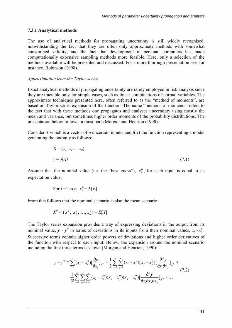
Methods of parameter uncertainty propagation and analysis
41
7.3.1 Analytical methods The use of analytical methods for propagating uncertainty is still widely recognised, notwithstanding the fact that they are often only approximate methods with somewhat constrained validity, and the fact that development in personal computers has made computationally expensive sampling methods more feasible. Here, only a selection of the methods available will be presented and discussed. For a more thorough presentation see, for instance, Robinson (1998). Approximation from the Taylor series Exact analytical methods of propagating uncertainty are rarely employed in risk analysis since they are tractable only for simple cases, such as linear combinations of normal variables. The approximate techniques presented here, often referred to as the “method of moments”, are based on Taylor series expansion of the function. The name “methods of moments” refers to the fact that with these methods one propagates and analyses uncertainty using mostly the mean and variance, but sometimes higher order moments of the probability distributions. The presentation below follows in most parts Morgan and Henrion (1990). Consider X which is a vector of n uncertain inputs, and f(X) the function representing a model generating the output y as follows:
X = (x1, x2 … xn)
y = f(X) (7.1) Assume that the nominal value (i.e. the “best guess”), 0
ix , for each input is equal to its expectation value: For i =1 to n, 0
ix = E[xi] From this follows that the nominal scenario is also the mean scenario: X0 = ( 0
1x , 02x , …, 0
nx ) = E[X] The Taylor series expansion provides a way of expressing deviations in the output from its nominal value, y - y0 in terms of deviations in its inputs from their nominal values, xi - 0
ix . Successive terms contain higher order powers of deviations and higher order derivatives of the function with respect to each input. Below, the expansion around the nominal scenario including the first three terms is shown (Morgan and Henrion, 1990):
K+∂∂∂
∂−−−
+∂∂
∂−−+∂∂−=−
∑∑∑
∑∑∑
= = =
= ==
n
i
n
j
n
kX
kjikkjjii
n
iX
jijj
n
jii
n
iX
iii
xxxyxxxxxx
xxyxxxx
xyxxyy
1 1 1
3000
1
20
1
0
1
00
0
00
])[)()((!3
1
])[()(21])[(
(7.2)

Uncertainty in Quantitative Risk Analysis – Characterisation and Methods of Treatment
42
It should be noted that all derivatives are evaluated for the nominal scenario X0. If the deviations xi - 0
ix are relatively small, the higher powers will become very small. And if the function is relatively smooth in the region of interest, the higher derivatives will be small. Under these conditions the Taylor series produces a good approximation even when the higher order terms are ignored. First order approximation In order to simplify the calculations, one usually only takes the first order term into consideration. To the first order, the expected value of y can be approximated by the nominal value, since the expected value of the deviation in y is zero: E[y – y0] ≈ 0, E[y] ≈ y0 = f(X0) (7.3) One can now obtain the general first order approximation of the variance in the output, using only the first order term from Eq. (7.2):
Var[y] = E[(y – y0)2] ≈
∂∂−∑
=
2
1
0
0
)(n
i Xiii x
yxxE
The above expression can, after some modifications and assumption of independence between the uncertain inputs (for the intermediate calculation steps, see Morgan & Henrion, 1990), be transformed to the simple Gaussian approximation formula given below:
Var[y] ≈ [ ]2
1 0X
i
i ii x
yxVar∑=
∂∂ (7.4)
As shown in the above equation, the variance of the output y is approximately the sum of the squares of the products of the standard deviation and sensitivity of each input, xi. This concludes this brief section on analytical methods of uncertainty propagation. More elaborative presentations are given by Morgan & Henrion (1990) and Robinson (1998). It is important, however, to remember that the formulas presented here are only approximations. They will not perform well in situations where the uncertainties are large. One can always try to improve the accuracy of the approximation by using higher order terms in the Taylor expansion, but then one must expect the complexity of the algebra to increase rapidly, especially when dealing with complex models, as is often the case in risk analysis. 7.3.2 Sampling methods Given the limitations of the analytical methods presented in the previous section, and the rapid development in personal computers, there has been a shift towards more computationally demanding, numerical methods for uncertainty analysis, allowing the use of full probability distributions to describe the uncertainty regarding parameters. In this section the basic features of two of these sampling procedures, Monte Carlo sampling and Latin hypercube sampling will be discussed. Bearing in mind that the sampling procedures

Methods of parameter uncertainty propagation and analysis
43
discussed here utilise the full distributions of the uncertain parameters for propagation, a technique for random sampling from these distributions must be established. In fact, this is essentially the difference between the two methods presented; they use different strategies for sampling from the input distributions. The presentation will be at a fairly basic level, focusing on the fundamentals of the methods and on principles of sound use in uncertainty analysis. The reader who is interested in hands-on examples of how these methods work is directed to the manuals of the many software packages that include these features, e.g. @Risk (Palisade Corporation, 2001). Monte Carlo sampling The oldest and best known sampling method still extensively employed in uncertainty analysis is the Monte Carlo sampling method. Vose (2000) gives an explicit presentation of how the method works, and here only the basic features are discussed. Let us start by defining the way in which the Monte Carlo procedure produces samples from the input distributions. Consider the cumulative distribution function F(x) for the uncertain variable X. It gives the probability P that the variable X will be less than or equal to x: F(x) = P(X ≤ x) F(x) ranges from zero to one. Let us consider the reverse of this equation, i.e. what is the value of F(x) for a certain value of x? The answer is given by the reverse function G(F(x)), which is written as follows: G(F(x)) = x In Figure 7.2 a graphical representation of the relationship between F(x) and G(F(x)) is given.
Figure 7.2. The relationship between x, F(x) and G(F(x)) (from Vose 2000). This is the concept used in the Monte Carlo sampling scheme for generating random samples from the distributions of the uncertain variables in the risk analysis model. To generate a random sample for a probability distribution, a random number, r, is generated between zero and one. This value is then fed into the equation to determine the value to be generated for the distribution:
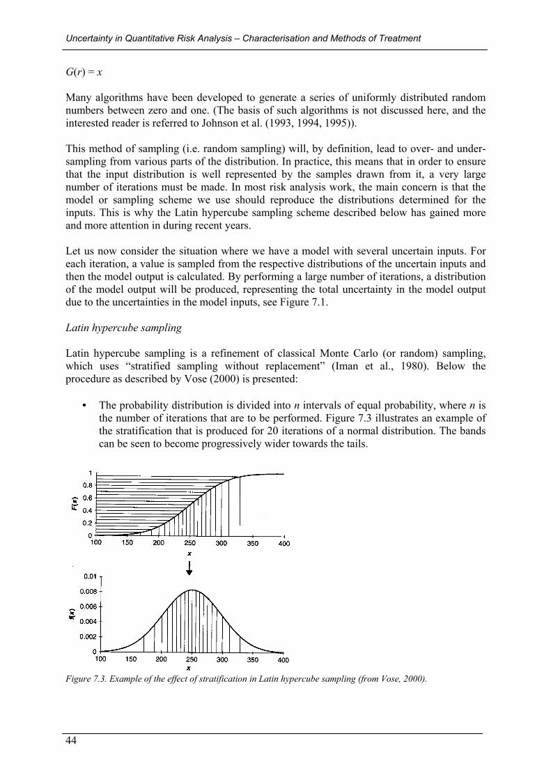
Uncertainty in Quantitative Risk Analysis – Characterisation and Methods of Treatment
44
G(r) = x Many algorithms have been developed to generate a series of uniformly distributed random numbers between zero and one. (The basis of such algorithms is not discussed here, and the interested reader is referred to Johnson et al. (1993, 1994, 1995)). This method of sampling (i.e. random sampling) will, by definition, lead to over- and under-sampling from various parts of the distribution. In practice, this means that in order to ensure that the input distribution is well represented by the samples drawn from it, a very large number of iterations must be made. In most risk analysis work, the main concern is that the model or sampling scheme we use should reproduce the distributions determined for the inputs. This is why the Latin hypercube sampling scheme described below has gained more and more attention in during recent years. Let us now consider the situation where we have a model with several uncertain inputs. For each iteration, a value is sampled from the respective distributions of the uncertain inputs and then the model output is calculated. By performing a large number of iterations, a distribution of the model output will be produced, representing the total uncertainty in the model output due to the uncertainties in the model inputs, see Figure 7.1. Latin hypercube sampling Latin hypercube sampling is a refinement of classical Monte Carlo (or random) sampling, which uses “stratified sampling without replacement” (Iman et al., 1980). Below the procedure as described by Vose (2000) is presented:
• The probability distribution is divided into n intervals of equal probability, where n is the number of iterations that are to be performed. Figure 7.3 illustrates an example of the stratification that is produced for 20 iterations of a normal distribution. The bands can be seen to become progressively wider towards the tails.
Figure 7.3. Example of the effect of stratification in Latin hypercube sampling (from Vose, 2000).

Methods of parameter uncertainty propagation and analysis
45
• In the first iteration, one of these intervals is selected using a random number. • A second random number is then generated to determine where, within that interval,
F(x) should lie. • x = G(F(x)) is calculated for that value of F(x). • The process is repeated for the second iteration but the interval used in the first
iteration is marked as having already been used and therefore will not be selected again.
• This process is repeated for all of the iterations. Since the number of iterations n is also the number of intervals, each interval will only have been sampled once and the distribution will have been reproduced with predictable uniformity over the range of F(x).
Two-phase sampling procedures In situations where it is desirable to keep different uncertainties separate in an analysis, for instance separating stochastic and epistemic uncertainty, “two-phase” sampling procedures are suitable. A two-phase sampling procedure is based on either traditional Monte Carlo sampling or another kind of sampling scheme, e.g. the Latin hypercube procedure described above. The procedure is conceptually relatively simple. The sampling is performed in two “loops”, an outer and an inner loop, to which the two different groups of uncertain parameters belong. For each iteration in the outer loop (where a value is sampled for all the parameters within the “outer loop” group), a specified number of iterations (in each of which a value is “drawn” for all the parameters in the “inner loop” group) is performed in the inner loop. For example, suppose we want to keep stochastic uncertainty and knowledge-based uncertainty separate in an analysis. Below is a description of the structure of one cycle in the outer loop. First we sample values for all of the parameters afflicted with knowledge-based uncertainty (the outer loop). These will be used while computing the model output in this cycle. Then we perform a specified number of iterations (say 10 000) in each of which we sample values for all the parameters afflicted with stochastic uncertainty (the inner loop). After each iteration in the inner loop we calculate the model output (using the same values for the outer loop parameters for all 10 000 iterations). The result will be a distribution which is governed solely by the uncertainty in the stochastic parameters. This procedure is repeated as many times as desire, each cycle producing one distribution. The final result will be a collection of distributions representing stochastic uncertainty, while the spread of distributions represents knowledge-based uncertainty, see Figure 7.4.
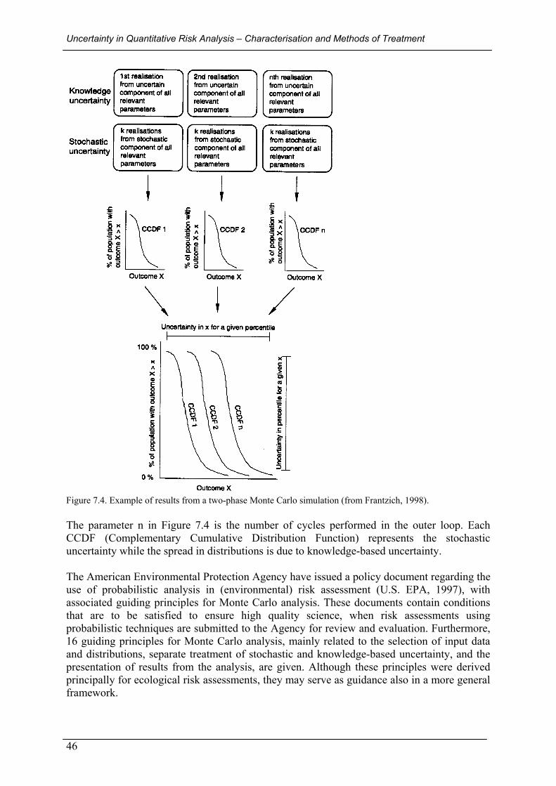
Uncertainty in Quantitative Risk Analysis – Characterisation and Methods of Treatment
46
Figure 7.4. Example of results from a two-phase Monte Carlo simulation (from Frantzich, 1998). The parameter n in Figure 7.4 is the number of cycles performed in the outer loop. Each CCDF (Complementary Cumulative Distribution Function) represents the stochastic uncertainty while the spread in distributions is due to knowledge-based uncertainty. The American Environmental Protection Agency have issued a policy document regarding the use of probabilistic analysis in (environmental) risk assessment (U.S. EPA, 1997), with associated guiding principles for Monte Carlo analysis. These documents contain conditions that are to be satisfied to ensure high quality science, when risk assessments using probabilistic techniques are submitted to the Agency for review and evaluation. Furthermore, 16 guiding principles for Monte Carlo analysis, mainly related to the selection of input data and distributions, separate treatment of stochastic and knowledge-based uncertainty, and the presentation of results from the analysis, are given. Although these principles were derived principally for ecological risk assessments, they may serve as guidance also in a more general framework.

Methods of parameter uncertainty propagation and analysis
47
7.4 Interval arithmetic The concept of interval arithmetic offers a computationally inexpensive, logically consistent methodology that produces conservative estimates of uncertainty in the final result of an analysis. Intervals have long been used in many disciplines to represent uncertainty. For instance, in empirical studies scientists are accustomed to reporting the measured values in terms of the best estimate and the possible error in the estimate in the form of an interval. Interval analysis can be used to propagate uncertainty concerned with input parameters (specified as intervals) through a model. An appealing feature of interval analysis is that it is fairly straightforward, which makes the methodology attractive, for example, in the screening phase of an analysis. In this section the basics of this arithmetic will be briefly discussed. For a more comprehensive presentation of interval analysis, see for instance Dwyer (1951), Moore (1966, 1979) or Alefeld & Herzberger 1983). Consider two variables X and Y, given as intervals [xl,xu] and [yl,yu] respectively, where xl ≤ xu and yl ≤ yu. The most basic arithmetic operations for intervals are given below: X + Y = [xl + yl, xu + yu] (7.5) X – Y = [xl - yu, xu - yl] (7.6) X · Y =[min(xlyl, xlyu, xuyl, xuyu), max(xlyl, xlyu, xuyl, xuyu)] (7.7) X / Y =[min(xl/yl, xl/yu, xu/yl, xu/yu), max(xl/yl, xl/yu, xu/yl, xu/yu)]; 0∉ [yl,yu] (7.8) Let us visualise this with a simple example (from Ferson et al., 1999). Suppose we know that the value of A is between 2 and 4, and that of a number B is between -1 and 3, which we represent by writing A=[2,4] and B=[-1,3]. Intuitively it is easy to see that the sum of A and B must be somewhere between 1 and 7, i.e. in the interval [1,7]. The endpoints of the resulting interval are the sums of respective endpoints of the inputs. However, as can be seen in Eq. (7.6), for subtraction the endpoints are the differences of the opposite endpoints of the inputs. In the example this would mean A - B = [-1,5], see Figure 7.5. A difference as low as -1 will arise from A being 2 and B being 3, and a difference as large as 5 will arise when A is 4 and B is -1.
A
1 2 3 4 5
B
-2 -1 0 1 2 3 4
A+B
0 1 2 3 4 5 6 7 8
A-B
-2 -1 0 1 2 3 4 5 6
A*B
-5 0 5 10 15
B/A
-1 -0.5 0 0.5 1 1.5 2 Figure 7.5. Examples of basic arithmetic operations on interval numbers.

Uncertainty in Quantitative Risk Analysis – Characterisation and Methods of Treatment
48
The product A · B must be in the interval [-4,12], see Figure 7.5. Notice that in this case finding the resulting interval is somewhat more complicated than simply finding the products of the endpoints of the factors. The lower bound of A is not even involved in the calculation of the result. As can be seen in Eq. (7.8), division is defined for interval numbers when the divisor does not contain zero within its range. Thus B/A exists, see Figure 7.5, but A/B does not. The example given above deals only with the most basic arithmetic operations: addition, subtraction, multiplication and division. The rules of interval analysis also allow us to compute bounds on all the elementary mathematical operations, for instance powers, roots, minima, maxima, exponentials and logarithms. Software for this kind of arithmetic is commercially available. Finally, it should be noted that interval analysis might seem somewhat paradoxical in that it implies that while one cannot know the exact value of a parameter, it is still fully feasible to know the bounds of the parameter exactly. This problem is addressed to some extent in fuzzy arithmetic, which is briefly introduced in Section 7.6. 7.4.1 Worst case analysis requires interval arithmetic It should be clear from the example above that interval arithmetic is an appropriate method of performing worst case analysis, i.e. estimating the upper (and by definition also the lower) bounds of the result as required in worst case analysis. Certainly, estimating the upper bound of a quantity, e.g. concentration or dose, by simply combining the upper bounds of all the variables in their respective deterministic expressions might lead to erroneous results, depending on the computational model structure. 7.4.2 Repeated parameters A problem in using non-deterministic measures (uncertain numbers) in arithmetic operations, which is easily seen in interval arithmetic, becomes apparent when the same parameter occurs more than once in an expression. For instance, consider the difference X-X: X - X = [x1, x2] - [x1, x2] = [x1 - x2, x2 - x1] ≠ 0 for situations where x1 ≠ x2, i.e. the cancellation law does not hold for intervals (with nonzero width). This result might seem somewhat peculiar at first and the explanation is given below. First, however, we shall consider yet another example of a variant of the problem. One of the basic laws of arithmetic on real numbers is called the distributive law of real numbers. Essentially, what it says is that X (Y + Z) = XY + XZ. We shall show that the distributive law does not always hold for uncertain numbers. Consider the numerical example:

Methods of parameter uncertainty propagation and analysis
49
X = [1, 3] Y = [2, 3] Z = [-1, 4] Alt. 1: X (Y + Z) = [1, 3] ([2, 3]+ [-1, 4]) = [1, 3] [1, 7] = [1, 21] Alt. 2: XY + XZ = [1,3] [2, 3] + [1, 3] [-1, 4] = [2, 9] + [-3, 12] = [-1, 21] As can be seen above the result is not the same for the two alternatives, i.e. the distributive law does not hold for intervals with negative inputs. It can be easily shown, however, that as long as the intervals are entirely positive, the distributive law holds. Furthermore, for all types of intervals, X (Y + Z) is always inside XY + XZ. It has been shown that neither the cancellation law nor the distributive law holds for all types of intervals. However, there are weaker laws for intervals: 0 ∈ X – X (7.9) X (Y + Z) ⊆ XY + XZ (7.10) Where ∈ means “is an element of” and ⊆ “is a subset of”. The essence of these laws is that an expression where X occurs several times might be wider than an expression where the Xs have been cancelled out. The obvious explanation is that interval analysis does not recognise and account for the dependence between the two Xs, i.e. repeating a parameter introduces the same uncertainty more than once in an expression. For this reason, the expression should be simplified, and any multiple occurrences of parameters should be cancelled out (whenever possible) before conducting interval analysis. In cases where repeated parameters cannot be cancelled out, the final result may show a greater uncertainty than would be expected. Despite this limitation, interval analysis may still be useful in the screening phase of an analysis, since the result will still enclose the true value. Finally, a word on the problems that repeated parameters might cause in other forms of uncertainty calculations. For reasons that will become apparent in the following section (where fuzzy arithmetic is regarded as a generalisation of interval analysis), the same problems will be experienced within the framework of fuzzy arithmetic. Furthermore, fuzzy arithmetic will show the same type of “fail-conservative” behaviour as interval analysis in that repeated parameters will always increase the uncertainty in the final result. The same type of problem could occur in Monte Carlo analysis, but within that framework a straightforward solution is feasible. For each iteration in the Monte Carlo procedure, one simply instantiates each occurrence of the parameter to the same value. For example, if the parameter X occurs twice in the expression analysed, the same value is used (in an iteration) at both positions in the expression.

Uncertainty in Quantitative Risk Analysis – Characterisation and Methods of Treatment
50
7.5 Probability bounds analysis In this section a relatively new approach to uncertainty propagation (Ferson et al., 1996, 1998) is briefly described. The most attractive feature of this approach, in my opinion, is that it provides a way of using the information available on a parameter to construct bounds on possible probability distributions without having to make any (unjustified) assumptions. With user-friendly software this approach provides a fairly simple tool for quality assurance of results from sampling based analyses, most of which often force the analyst to make (sometimes questionable) assumptions about the distributions of the parameters and dependencies and correlations between the parameters in the model expression. The basic features of the probability bounds approach are presented below. Probability bounds may be constructed from parametric probability distributions, where the parameters of the distributions are uncertain. For example, parameter X is a log-normal distribution with a mean µ = [2.5,3] and standard deviation σ = [0.8,1]. In Figure 7.6, the bounds on all possible distributions given this information are displayed for parameter X. Probability bounds can also be constructed in a distribution-free context, where one cannot specify the particular shape of a distribution. For instance, all that is known about parameter Y is its min = 2, max = 3 and mean = 2.4. Nothing is known about the shape of the distribution. In Figure 7.6, the bounds on all possible distributions given this information are displayed for parameter Y. The software RiskCalc (Ferson et al., 1999) was used to generate the probability bounds in this example. Distribution-free probability bounds have been derived for various sets of information regarding the uncertain variable, see Ferson et al. (1999). Z is a uniform distribution with min = 2 and max = 3. All Parameters are shown as cumulative distribution functions.
X
0
0.2
0.4
0.6
0.8
1
0 2 4 6 8
x
P(X)
< x
Y
0
0.2
0.4
0.6
0.8
1
1.5 2 2.5 3 3.5
y
P(Y)
< y
Z
0
0.2
0.4
0.6
0.8
1
1.5 2 2.5 3 3.5
z
P(Z)
< z
X+Y+Z
0
1
4 6 8 10 12 14t
P(X+
Y+Z)
< t
Figure 7.6. Examples of the addition of probability bounds. In the lower right corner of Figure 7.6, the parameters X, Y and Z have been added assuming independence (the bold lines). If one is uncertain about dependencies between the variables

Methods of parameter uncertainty propagation and analysis
51
the probability bounds approach allows arithmetic operations where no assumptions about dependencies are made (Ferson et al., 1999). The fine lines in the lower right corner of Figure 7.6 show the result of addition where no assumptions about dependencies have been made. Obviously, without the assumption of independence, the uncertainty band is wider. Probability bounds may be used in calculations wherever probability distributions can be used. For more details on the mathematical foundations of the probability bounds approach see, for instance, Ferson et al., (1996, 1999).
7.6 Fuzzy arithmetic Fuzzy arithmetic can be regarded as a generalisation of interval analysis in that a fuzzy number can be considered to be a nested stack of intervals, each at a different level of presumption α, 0 ≤ α ≤ 1, see Figure 7.7. The range of values is widest at a presumption or ‘possibility’ level of zero. Just above α level zero is the interval that everyone would agree contains the true value, i.e. the most conservative range. At an α level of one the most optimistic range of values is given. This range may even be a point, i.e. the best estimate of the value. It is also possible to consider the α level in the following way: α = 1 is the range of values that are identified as “entirely possible”, while in contrast just above α = 0 is the range of values that are “just possible” or only “conceivable” (Ferson & Kuhn, 1994). Zadeh first introduced the concept of fuzzy sets in 1965 (Zadeh, 1965). Since then, several thousands of papers and books have been published on the subject. Fuzzy arithmetic is an offshoot from fuzzy set theory and the rules for combining fuzzy numbers in calculations are given within this framework. The arithmetic of fuzzy numbers, as described by Kaufmann and Gupta (1985), essentially reduces to interval analysis repeated once for each α level. The difference is that fuzzy arithmetic generates an entire distribution instead of a simple interval or range. In the examples shown below the software RiskCalc 3.0 (Ferson et al, 1999) has been used to demonstrate some basic arithmetic operations on fuzzy numbers. As for intervals, most arithmetic operations, including powers, roots, minima, maxima, exponentials and logarithms, are defined for fuzzy numbers, and a wide range of software for performing fuzzy arithmetic is commercially available.
A
0
0.5
1
1 2 3 4 5
α
B
0
0.5
1
-2 0 2 4 6
α
A+B
0
0.5
1
0 1 2 3 4 5 6 7 8 9
α
A-B
0
0.5
1
-4 -2 0 2 4 6
α
A*B
0
0.5
1
-5 0 5 10 15 20
α
B/A
0
0.5
1
-1 0 1 2 3
α
Figure 7.7. Examples of basic arithmetic operations on fuzzy numbers. Fuzzy numbers in the sense described above have been used to some extent to represent uncertainty in various risk analysis applications in the past 10-20 years. For example, Schemel et al. used fuzzy numbers to represent uncertainty in failure probabilities in fault trees

Uncertainty in Quantitative Risk Analysis – Characterisation and Methods of Treatment
52
regarding the reliability of foam suppression systems (Schemel et al., 2000). Abrahamsson et al. made use of fuzzy numbers to represent uncertainty in probabilities in a decision-making situation regarding which level of fire protection to use in an industrial facility (Abrahamsson et al., 2001). Ferson & Kuhn used fuzzy numbers to propagate uncertainty in ecological risk analysis (Ferson & Kuhn, 1992). There is an immense body of literature on this matter available for the interested reader. The main argument for using fuzzy numbers and fuzzy arithmetic over the more classical probabilistic approach in risk analysis is that it is claimed to “make fewer assumptions” than probability theory, principally because it is based on weaker axioms. Obviously, no one can argue against probability theory possibly proving more powerful in situations where all of its axioms are satisfied but, it is claimed that risk analysis is often performed in situations where, for example, access to data is severely limited. In a classical example of how probability theory and fuzzy arithmetic differ, Ferson et al. compare the sums of uniform distributions (Ferson et al., 1999): “When two uniform probability distributions are added together under the assumption of independence, the result is a triangular distribution. In the limit, the sum tends to a normal distribution (with a very small coefficient of variation). When two analogous flat fuzzy numbers (i.e. intervals) are added together, the result is another flat distribution, and in the limit, still a flat distribution. The big difference here is that fuzzy arithmetic is not assuming independence between the variables. Of course, when the input distributions are not flat, the answer coming out of fuzzy arithmetic won’t be either, but the distribution will be broader than that predicted by the comparable probabilistic method. However, it won’t be as broad or hyper conservative as the analogous interval or worst case method. Likewise, because fuzzy numbers are fashioned merely as robust representations of existing uncertainty, there should only be weak sensitivity of the final results to details of the shapes of the input distributions. Many analysts consider this an important advantage because there is often so little dependable empirical information underlying the selection of one input distribution over many alternatives. It’s fair to say that fuzzy arithmetic is intermediately conservative between Monte Carlo analysis and worst case/interval analysis.” It should not be forgotten that fuzzy arithmetic is still considered controversial by a “non-negligible” part of the risk analysis and decision theory community, see for instance Cooke (1991). In Ferson et al. (1999) the following comments are made: “/…/ it is true however that possibility theory and fuzzy arithmetic are young disciplines. There has not been very much time for theorists and practitioners to amass a long tradition of experience from which risk analysts might draw guidance. Nevertheless, the many advantages of fuzzy arithmetic suggest it can be very useful for risk assessments where data are perennially in short supply.”
Methods of parameter uncertainty propagation and analysis
53
7.7 Arguments for and against the different approaches to uncertainty analysis It is my firm belief that it is impossible to identify a single approach to uncertainty analysis that will prove to be the most powerful in all situations. The choice of approach is a delicate one and will most certainly be dependent on factors such as the purpose of the risk assessment, the information at hand, the nature of the uncertainty, e.g. variability or ambiguity etc. In this section, an effort is made to present the most obvious pros and cons regarding the different methodologies that have been presented in the previous sections. I believe that it will always, to some extent, be a matter of opinion which method is most appropriate in a given situation. Indeed, the differences between the methods are substantial, and the choice of method may significantly influence the final result of the risk assessment. It might at times prove wise to employ more than one methodology for a particular situation, perhaps at different times during the process, e.g. interval analysis in the screening phase and some other method for the more detailed analysis, or to answer different questions or address different problems. 7.7.1 Deterministic (best estimate) approach Pros: The results will represent the best estimate of the risk, hopefully producing more realistic results than, for instance, worst case analysis. Cons: This approach does not express the reliability of the results. To make sound use of this approach it would have to be combined with other types of information including the effects of uncertainties. 7.7.2 Worst case analysis Pros: Worst case analysis accounts for uncertainty by being conservative and it might prove especially useful in screening assessments. Cons: It will be very difficult, if not impossible, to be consistent regarding how conservative different analyses are, which makes it impossible to compare risks from different analyses. There is a good chance that the analysis will be hyper-conservative, which makes it impossible to make sound decisions on, for instance, risk-reducing measures under economical constraints. 7.7.3 Interval analysis Pros: Interval analysis is a straightforward, easily explainable, method that in fact generalises and refines worst case analysis. Interval analysis can be used whatever the source of uncertainty. Interval analysis is very well suited for screening studies, due to inherent conservatism and simplicity. Cons: Since one is working with only the ranges of the inputs, these ranges can grow very quickly, making the results more or less useless in many real-life situations. There is no way to take into account more information on the parameters than just the ranges, which will often lead to too conservative results. To some extent, the approach is paradoxical, since it implies that one cannot know the exact value of a parameter, but the exact bounds may be known. The methodology compounds stochastic and knowledge-based uncertainty.
Uncertainty in Quantitative Risk Analysis – Characterisation and Methods of Treatment
54
7.7.4 Fuzzy arithmetic Pros: Fuzzy arithmetic can be regarded as a generalisation of interval analysis, making computations easy and easy to explain. (Software is required for non-elementary problems). The methodology does not require detailed empirical information; one can make use of subjectively assigned distributions. Fuzzy numbers are robust representations of uncertainty when empirical information is very sparse. Dependencies and correlations between parameters need not be specified as the methodology is inherently conservative in this matter. Cons: Fuzzy arithmetic is not yet widely known in the risk analysis community, and some criticism has been directed towards the fundamentals of the methodology. The meaning of α, i.e. the level of conservatism is not clear. This poses problems since one might use different levels of conservatism for different parameters in an analysis. Although it is not as conservative as interval analysis, it might still be too conservative in some situations. One could say that the approach is intermediate regarding conservatism between analogous Monte Carlo and interval approaches. As with interval analysis, repeated parameters may constitute a computational problem, leading to unnecessarily conservative results. There is as yet no method for merging fuzzy arithmetic with Monte Carlo-based methods, which possibly would have been an advantage since some argue that fuzzy numbers handle certain types of uncertainty better than Monte Carlo methods and vice versa. No methods are available within the fuzzy framework to keep different types of uncertainty separate in an analysis. 7.7.5 Analytical probabilistic analysis Pros: For simple models where the uncertainties are small, Gaussian approximation methods have proved to be useful. The approach is fairly simple and has a long tradition in, for instance, the physical sciences. It usually requires only the mean and variance, i.e. one does not have to specify the total distribution. One of the most appealing features of this approach is that the importance of each parameter in the model, with respect to its contribution to the overall uncertainty, is given directly since the variance of the model output is expressed as the sum of the variances of each input. Cons: The uncertainties in risk analysis are often large compared with nonlinearities in the models, making these first-order approximations less suitable. Higher order approximations could be used to help solve this problem, but this often leads to complicated algebraic solutions when the models grow in complexity, which is often the case in risk analysis. Since the method only requires the mean and variance as input, these are also what is obtained as output. This could be a problem, especially when the tails of the distributions are of interest in the risk analysis, e.g. in the analysis of systems characterised by low probability, high consequence scenarios.

Methods of parameter uncertainty propagation and analysis
55
7.7.6 Monte Carlo analysis (including Latin hypercube and other sampling schemes) Pros: The sampling-based methodologies described earlier are all fairly simple to implement, equally simple to explain, and user friendly software is available for analysts. When used correctly, the total distributions of the model output are obtained, representing the full uncertainty in the model output. Within this framework, one can use information on correlations and dependencies between the variables to see what impact they have on the uncertainty in the final results. Cons: To be able to perform a Monte Carlo analysis, one has to have access to a great deal of empirical information, e.g. explicit information on the distributions of all variables and their correlations and dependencies. In practice, this often forces the analyst to make (sometimes questionable) assumptions regarding, for instance, independence, which might lead to non-protective results, i.e. the output distributions are “narrower” than justified. Within the classical Monte Carlo approach, it is not possible to separate different kinds of uncertainties, i.e. stochastic uncertainty and knowledge-based uncertainty are combined. 7.7.7 Two-phase Monte Carlo analysis Pros: The most obvious advantage of two-phase Monte Carlo methods over standard methods is that it is possible to distinguish between different kinds of uncertainty, i.e. uncertainty due to natural variability (stochastic uncertainty) and uncertainty due to a lack of knowledge (epistemic uncertainty). Within this framework it is possible to express and account for uncertainty in the parameters of the chosen distributions for the input variables. The methodology provides a way of handling model uncertainty. When carried out correctly, this is the perhaps most powerful method of uncertainty propagation and analysis. Cons: Although this methodology deals with uncertainty in the parameters of the distributions it is not capable of handling uncertainty in distributional shapes. In complex models, the calculations can be cumbersome and the computational requirement grows rapidly. 7.7.8 Probability bounds analysis Pros: The most attractive feature of this approach is that it can deal with uncertainty in parameter values, distribution shapes, dependencies (in a conservative way) and model form. One can make use of newly gained empirical information to tighten the bounds, thus reducing the uncertainty in the final result. This approach provides a simple means of quality assurance of Monte Carlo results. Cons: The only way to present the results is in cumulative form. It is difficult to obtain optimal bounds when there are repeated occurrences of parameters in the expression. One cannot use information on correlations and dependencies (apart from independence assumptions) to tighten the bounds. The methodology can not be used to separate different kinds of uncertainties.
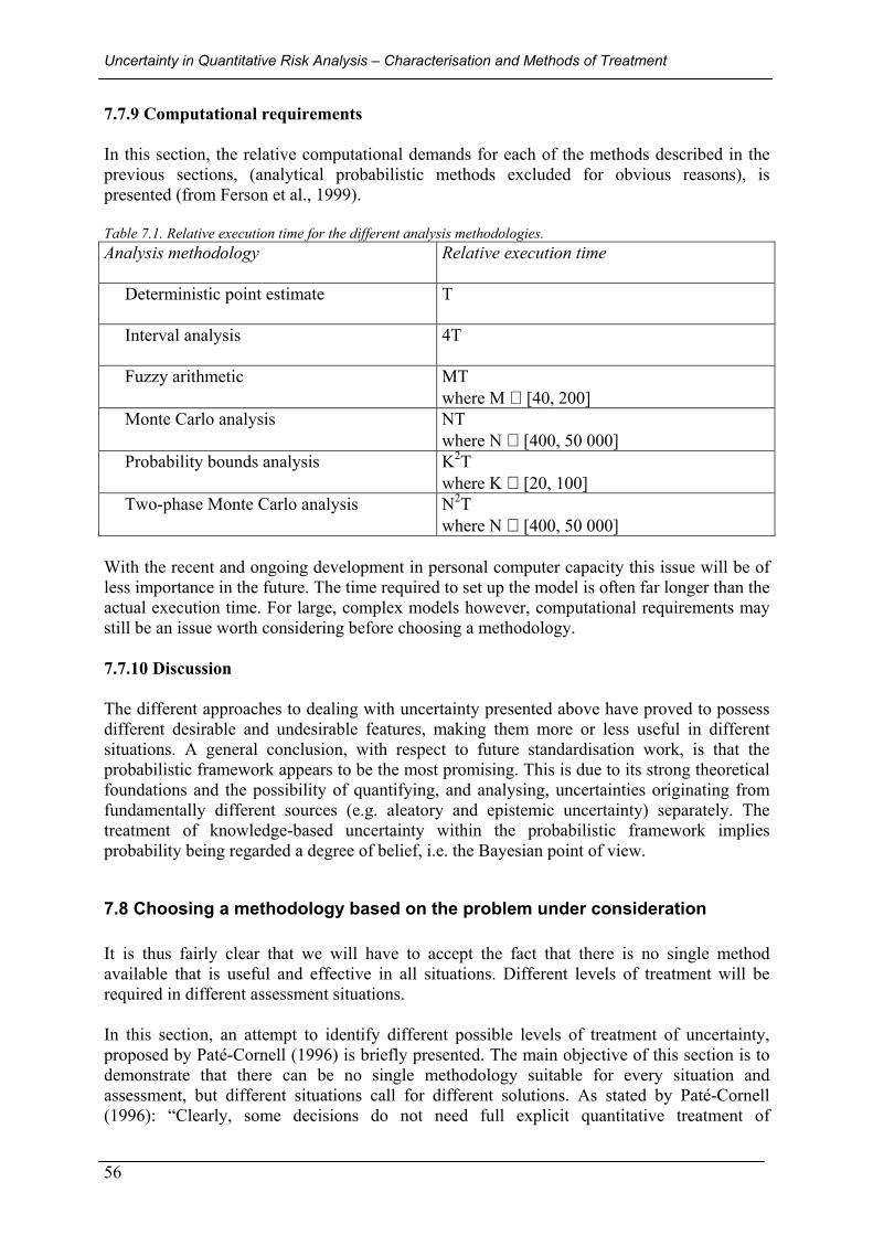
Uncertainty in Quantitative Risk Analysis – Characterisation and Methods of Treatment
56
7.7.9 Computational requirements In this section, the relative computational demands for each of the methods described in the previous sections, (analytical probabilistic methods excluded for obvious reasons), is presented (from Ferson et al., 1999). Table 7.1. Relative execution time for the different analysis methodologies. Analysis methodology
Relative execution time
Deterministic point estimate
T
Interval analysis
4T
Fuzzy arithmetic MT where M ∈ [40, 200]
Monte Carlo analysis NT where N ∈ [400, 50 000]
Probability bounds analysis K2T where K ∈ [20, 100]
Two-phase Monte Carlo analysis N2T where N ∈ [400, 50 000]
With the recent and ongoing development in personal computer capacity this issue will be of less importance in the future. The time required to set up the model is often far longer than the actual execution time. For large, complex models however, computational requirements may still be an issue worth considering before choosing a methodology. 7.7.10 Discussion The different approaches to dealing with uncertainty presented above have proved to possess different desirable and undesirable features, making them more or less useful in different situations. A general conclusion, with respect to future standardisation work, is that the probabilistic framework appears to be the most promising. This is due to its strong theoretical foundations and the possibility of quantifying, and analysing, uncertainties originating from fundamentally different sources (e.g. aleatory and epistemic uncertainty) separately. The treatment of knowledge-based uncertainty within the probabilistic framework implies probability being regarded a degree of belief, i.e. the Bayesian point of view.
7.8 Choosing a methodology based on the problem under consideration It is thus fairly clear that we will have to accept the fact that there is no single method available that is useful and effective in all situations. Different levels of treatment will be required in different assessment situations. In this section, an attempt to identify different possible levels of treatment of uncertainty, proposed by Paté-Cornell (1996) is briefly presented. The main objective of this section is to demonstrate that there can be no single methodology suitable for every situation and assessment, but different situations call for different solutions. As stated by Paté-Cornell (1996): “Clearly, some decisions do not need full explicit quantitative treatment of
Methods of parameter uncertainty propagation and analysis
57
uncertainties (or any at all): sound risk management decisions are often made and have been made for a long time without any such analysis. In other cases, an analysis is extremely helpful because the problem is complex and the information needs to be structured.” An attempt is made here to relate the different levels of treatment proposed by Paté-Cornell to the methods presented earlier in this chapter. Level 0: Identification of hazard Level 0 involves the identification of a potential hazard or of the different ways in which a system can fail, without attempting to assess the risk in any quantitative way. This level of analysis can be sufficient to support zero-risk policies, or to make risk management decisions when the costs are low and the decision is clear. Not many practical decision-making situations in the area under consideration fit this description, however. Level 1: “Worst-Case” approach Level 1 is the “worst-case” approach. This approach does not consider the probability or possibility of different outcomes. It is based on the accumulation of worst-case assumptions and yields, in theory, the maximum loss level. The approach is reasonable if knowing the worst possible loss is sufficient to support the decision. Worst-case analysis requires interval analysis for reasons described in Section 7.4.1. However, in practical decision-making situations this approach is rarely of any real value, since regardless of how the worst-case scenario is constructed, it will always be possible to imagine (even more unlikely) events that will worsen the results. This is partly why the “quasi-worst case” has been a dominant approach in many engineering disciplines as the main method of accounting for uncertainty, see below. Level 2: Quasi-worst-case, plausible upper bounds Level 2 involves “plausible upper bounds”. This analysis represents an attempt to obtain a deterministic evaluation of the worst possible conditions that can “reasonably” be expected when there is either some uncertainty as to what the worst case might be, or when the worst case is so unlikely that it is meaningless. This is, by far, the most common approach in many engineering disciplines, e.g. fire safety engineering, to account for uncertainty in design situations. For example, when evaluating the fire safety in public buildings, the predominant methodology is to construct “design fire scenarios” using a quasi-worst-case approach. The method best suited for this level of treatment of uncertainty would be interval analysis. However, major shortcomings in the quasi-worst-case approach become apparent when decisions have to be made under budget constraints, e.g. a choice between different design alternatives, since there is no way of evaluating and comparing the level of conservatism in the different alternatives. Furthermore, comparison of risks based on the plausible upper bounds approach will not be meaningful, since there is no theoretical reason for the ranking of risks according to plausible upper bounds to be the same as the ranking of the means (Paté-Cornell, 1996). In this respect, a “best estimate” approach is more promising. Level 3:”Best estimate”, central value Level 3 analysis involves a “best estimate” and/or on a central value (e.g., the mean, the median or the mode) of the outcome distribution, generally obtained by using “best estimates” of the different variables. This approach is often used in applications such as cost-benefit
Uncertainty in Quantitative Risk Analysis – Characterisation and Methods of Treatment
58
analysis. “Generally speaking, the advantage of central values is to provide a reasonable balance to plausible upper bounds” (Paté-Cornell, 1996). However, this kind of deterministic approach does not provide a sufficient description of the effects of uncertainties on the results. Level 4: Probabilistic risk assessment, single risk distribution It is first on this level that one can talk of quantitative risk analysis as defined in Chapter 2. It is within this group that most of the methods presented earlier in this chapter belong. (The term used by Paté-Cornell implies that only the probabilistic approach is valid, but if one accepts the fuzzy framework, it provides this level of treatment.) The approach is based on generating a distribution of the possible outcomes, where aleatory and epistemic uncertainties are aggregated into one single distribution. (It should be noted, however, that when performed in its simplest form, QRA provides a distribution of the probabilities of different system states based on best estimates of the models and parameter values, involving only aleatory uncertainties.) The approach in which different types of uncertainty are aggregated into one distribution is sufficient if one is interested only in a full representation of all the uncertainties involved in an analysis, and not in whether the uncertainties originate from randomness or lack of knowledge. (The probability bounds approach described in Section 7.5 can be regarded a special case in this group, since it provides bounds on all the possible distributions of the outcome, but still aggregates stochastic and knowledge-based uncertainty.) Obviously, if one is interested in finding ways of reducing the total uncertainty in the results, it may be helpful to keep different types of uncertainty separate in an analysis, see below. Level 5: Separation of different types of uncertainty Level 5 constitutes the most sophisticated treatment of uncertainty, since fundamentally different types of uncertainty, i.e. randomness and epistemic uncertainty, are kept separate during the analysis; for a practical example, see Chapter 9. The main methods capable of this kind of analysis are the analytical probabilistic methods (for simple problems), and two-phase Monte Carlo procedures. The results obtained from such an exercise will be a family of distributions of the output, where each distribution represents stochastic uncertainty, and the dispersion of the distributions represents the effects of epistemic uncertainty. Let us conclude this section with the words of Paté-Cornell (1996): “In all cases, it is essential to remember how the numbers were generated, what they represent and what they can be used for.”

Methods of ranking uncertain parameters
59
8. Methods of ranking uncertain parameters One of the major objectives in performing a complete parameter uncertainty analysis is to rank the parameters with respect to their contributions to the uncertainty in the model prediction (IAEA, 1989; Morgan & Henrion, 1990). The most obvious reason for this being that such a ranking makes it possible to allocate research resources efficiently, should a reduction in the calculated uncertainties in the output prove necessary in order to reach an acceptable degree of reliability in the results. Of course, the methods available for this kind of ranking will be dependent on the type of uncertainty propagation method used, e.g. if analytical or numerical methods have been used. In this section, only methods within the probabilistic framework will be described. Some suggestions have been made regarding methodology for importance measures within a “fuzzy” framework. None of these are, however, discussed here, partly due to lack of consensus regarding appropriate methods in the literature. The interested reader is directed towards Suresh et al. (1996) and Furuta & Shiraishi (1984) where fuzzy importance measures in fault tree analysis are discussed.
8.1 Analytical methods The probabilistic analytical methods of uncertainty propagation discussed in Section 7.3.1 provide the variance of the model prediction as a function of the variances and covariances of the uncertain parameters, and an immediate ranking of the individual parameters with respect to their contribution to the overall uncertainty in the model prediction is thus possible.
8.2 Numerical methods In this section some of the most commonly employed indicators for ranking uncertain parameters in relation to sampling-based methods for uncertainty analysis and propagation will be presented. 8.2.1 Correlation coefficients One fairly simple and straightforward method of ranking uncertain parameters is to calculate the sample correlation coefficient of the model prediction and each of the uncertain parameters, using the sample of output values and the corresponding sample of values for each input. Consider n samples from the output and a single input, denoted as yj, xj, for j = 1 to n. The sample (or Pearson) correlation coefficient is computed from:
∑ ∑
∑
= =
=
−⋅−
−⋅−=
n
j
n
jjj
n
jjj
XY
yyxx
yyxxr
1 1
22
1
)()(
)()( (8.1)

Uncertainty in Quantitative Risk Analysis – Characterisation and Methods of Treatment
60
The correlation coefficient provides an estimate of the degree of linear relationship between the sample values of the model output and the input parameter. This is done for every input parameter, providing a measure of how much each input contributes to the output uncertainty. The sign of the coefficient tells us the direction of the relationship, and the absolute value of the coefficient indicates the strength of the relationship (where -1 indicates a completely negative linear relation and +1 a completely positive linear relation). In situations often encountered in risk analysis, where there are significant correlations between the input parameters, the correlation coefficient measure fails to recognise these correlations. For example: the contribution from an uncertain parameter to the total uncertainty in the output is insignificant. It is, however, strongly correlated another input parameter, which is a major contributor to the output uncertainty. In this case, the correlation coefficients computed for the two input parameters will be almost the same in absolute terms (IAEA, 1989). However, Iman and Helton (1988) show how to compute partial correlation coefficients, which eliminates the effect of correlated inputs. 8.2.2 Partial correlation coefficients As stated above, the correlation coefficient measure does not account for correlations between the input parameters. Partial correlation coefficients (PCC) are, however, measures of the contribution of each input parameter to the total output uncertainty, after effects attributable to other input parameters have been removed (Morgan and Henrion, 1990). See the IAEA report (1989) for information on how to calculate the PCC. However, the IAEA report (1989) indicates several limitations regarding the usefulness of this measure in ranking uncertain parameters. For instance, it is not possible to obtain an estimate of how much of the final variation in the model output can be explained by a linear relationship between the uncertain parameters and the model output in the nonlinear case, which makes a discussion about linear regression and standardised regression coefficients necessary. 8.2.3 Multiple linear regression analysis A linear regression model of Y as a function of X assumes that a linear relationship of the type Y = a + bX + ∈ holds, where ∈ is a random error (IAEA, 1989). Basically, the model tries to fit a straight line to data consisting of the values y1, y2, … , yn observed for given values of x1, x2, … , xn by obtaining estimates of the coefficients a and b. (See IAEA (1989), or any standard textbook on statistics for a detailed description of the linear regression procedure.) In the case of multiple linear regression the assumed linear expression for Y is not just a function of one variable, X, but of several variables X1, X2, … , Xm. The resulting approximate expression is often called a “fitted response surface”. For a practical example of the response surface method, see Frantzich, Harrada & Magnusson (1995). When performing a multiple regression analysis, it is common practice to calculate the sample coefficient of determination R2 (see, for instance, IAEA (1989) for guidance on how to calculate R2), which is an indication of how much of the variation in the model output is explained by a linear relationship to the uncertain parameters included in the regression expression. This is very useful since it provides an indication on how much confidence we may have in the ranking of the uncertain parameters generated by the regression analysis.
Methods of ranking uncertain parameters
61
Partial regression coefficients The coefficients ai, i = 1, 2, … , m of a multiple linear regression model,
Y = a0 + a1X1 + a2X2 + … + amXm + ∈ (8.2) are called partial regression coefficients. They are by definition the partial derivates of Y with respect to Xi. The practical meaning of this is that the coefficient ai indicates the change in model output Y associated with a unit change in Xi, all other Xk, k ≠ i remaining constant, making the coefficients in some sense suitable for ranking the uncertain parameters, (together with the sample coefficient of determination, R2). One problem, however, is that this measure is sensitive to the units of the uncertain parameters. This problem is eliminated by calculation of the standardised partial regression coefficients. Standardised partial regression coefficients If, in the multiple regression model presented in the previous section, Y and Xi are standardised according to:
V = (Y – E(Y)) / D(Y), Ui = (Xi – E(Xi)) / D(Xi) then the coefficients bi, i = 1, 2, … , m of the multiple linear regression model
V = b1U1 + b2U2 + … + bmUm + ∈ (8.3) are called standardised partial regression coefficients. The practical meaning of this is that the coefficient bi indicates by how many standard deviations the model output Y changes when Xi changes by one standard deviation, all other Xk, k ≠ i remaining constant. This, together with the sample coefficient of determination R2, makes the standardised partial regression coefficients very illustrative measures for ranking uncertain parameters. 8.2.4 Rank correlation coefficients One limitation of correlations and regression coefficients in ranking uncertain parameters is that they are generally not good indicators of nonlinear monotonic relationships between input and output. This, however, is not at all surprising since regression and correlation analyses are in fact based on developing linear relationships between variables. To overcome the problems associated with poor linear fits to nonlinear data one can use a rank transformation procedure, in which the original data are replaced by their corresponding ranks, and the normal regression and correlation procedures are then performed on these ranks. The procedures are explicitly described by Saltelli & Sobol (1995). Basically, the rank transformation itself is nothing more than a process of arranging a set of values in ascending order and assigning an ordinal number to each value, for example:
Uncertainty in Quantitative Risk Analysis – Characterisation and Methods of Treatment
62
Given set Corresponding rank of values transformed values
-2.4 3 -7.2 5 -2.7 1 -3.8 4 -0.5 2 The sample correlation coefficients of the rank transforms of the model prediction and each of the uncertain parameters are called sample rank correlation coefficients (RCCs). Rank correlation coefficients are considered to be more generally suitable for ranking uncertain parameters than indicators of degrees of linear relationship only, such as the correlation coefficients and standardised partial regression coefficients described in the previous sections. It was shown above that the correlation coefficient can be found via the partial correlation coefficient to finally reach the standardised partial regression coefficient, which proved to be a more effective indicator for ranking uncertain parameters due to (among other things) its insensitivity to the units of the uncertain parameters and the possibility of checking how good an indicator it really is by calculating the sample coefficient of determination R2. In a similar manner one can argue for a transition from the rank correlation coefficient, via the partial RCC to the standardised partial rank regression coefficient (SPRRC) to reach a more generally applicable indicator for ranking uncertain parameters. IAEA (1989) describes the process of obtaining the SPRRCs as follows. “To obtain the SPRRCs from a given random sample of parameter values and corresponding model predictions the sample values are first rank transformed and then standardised. Multiple linear regression performed on these rank transformed and standardised values provides the SPRRCs. The corresponding value of R2 indicates how much of the variation of the rank transformed sample values of the model prediction is explained by a linear relationship to the rank transforms of the uncertain parameters.” In situations where the underlying data do not show monotonic relationships (where, by definition, correlation and regression methods perform poorly, whether rank transformed or not), Helton & Davis suggest sampling based methods for identification of nonmonotonic patterns and random patterns. These methods are not discussed here and the interested reader is referred to Helton & Davis (2000).

Case study
63
9. A case study In this section, a simple case study will be presented, in which the different features of the methods of uncertainty propagation surveyed are highlighted. The example involves a simplified pressurised ammonia storage facility, consisting of a pressurised tank and 3 metres of pipeline (∅ 50 mm). The assessment will consider the release of pressurised ammonia to the surroundings, and the assessment end-points are:
• Concentration of ammonia at a geographical location (x,y), see Figure 9.1. • Individual risk (as defined in CCPS 2000) at a geographical location (x,y). • Societal risk (as defined in CCPS 20008) at a geographical location (x,y).
The different methods of uncertainty propagation described earlier have been used for each of these end-points. For comparison, the installation was also analysed using the Dutch approach described by the Committee for the Prevention of Disasters in the report CPR18E (1999).
Figure 9.1. Overview of the assessment case. The delimited system, consisting of a pressurised tank and 3 metres of pipe, and the calculation grid used in the example. In the example, three different physical models are used, i.e. a discharge model for estimating the source term, a dispersion model for estimating the concentration of ammonia at a specific geographic point (i.e. the grid point), and a Probit function to represent the dose-response relationship. The (fairly simple) models used in this example are all in the form of analytical expressions (see Appendix 3), which is a prerequisite for the use of most of the methods of uncertainty propagation described earlier. The objective of this example is to demonstrate the various features of the methods of uncertainty propagation, not to model the situation as accurately as possible. (When more complex computer models are used for the physical modelling, response surface methods are available, producing analytical expressions, based on
8 For the calculation of individual and societal risk, the general approach is to define a grid over the area of interest, i.e. the calculation grid. For the calculation of societal risk, the population density in each grid cell is assumed to be condensed in the grid point (i.e. the central point of the grid cell). Thus, calculations have only to be made for the grid point.

Uncertainty in Quantitative Risk Analysis – Characterisation and Methods of Treatment
64
a few variables, to represent the computer models, see Section 7.1.1.) Furthermore, model uncertainty is not explicitly treated, except for one isolated example in Section 9.2.2, where model uncertainty is used to exemplify the features of two-phase Monte Carlo analysis.
9.1 Extended QRA - Definition of possible incidents/scenarios Inherent in the QRA methodology is the identification of possible accident scenarios. In the Dutch guidelines for QRA, described by the Committee for the Prevention of Disasters (1999), the loss of containment (LOC) events required to be included in an analysis are prescribed for various equipment9. Below the prescribed LOCs for the equipment analysed in this example are shown. These will be used throughout the example, without further efforts to identify additional possible LOCs. Thus, completeness uncertainty in this respect is not analysed in the example.
T1: instantaneous release of the complete inventory of the tank, T2: continuous release of the complete inventory in 10 min at a constant rate of release, T3: continuous release from a hole with an effective diameter of 10 mm, P1: full bore rupture of the pipe, P2: outflow from a leak with an effective diameter of 10% of the nominal diameter of the pipe, and a maximum of 50 mm.
In the following examples, some of the parameters in the above scenarios, for instance, the time required to empty the tank in LOC T2 will be treated as uncertain variables, in order to exemplify how the different methods of uncertainty propagation work, and what kind of result they produce. In the example, no formal methods have been used when establishing the representation of uncertainty for the variables under consideration. However, as stated above, the main objective of the example is to present the features of the different methods of uncertainty propagation and analysis rather than to try to model the situation as correctly as possible.
9.2 Concentration at grid point (300,0) In this section, the average concentration of ammonia at grid point (x,y), following a discharge, will be calculated, where x is the downwind distance from the discharge to the geographical point of interest, and y is the cross-wind distance from the centre of the gas plume. In the example x is set to 300 m and y is set to 0 m. 9.2.1 A single LOC Let us consider one single LOC, for instance T2 in the list above. The concentration at grid point (300,0) is calculated for a number of different weather conditions, i.e. different stability classes10 and wind speeds.
9 It should be noted that when prescribing the LOCs to be used in an analysis, the issuer of such guidelines, by some means, accepts responsibility for any completeness uncertainty introduced during the identification stage of an analysis. 10 For a description of atmospheric stability classes see, for instance, CCPS (2000).

Case study
65
The Dutch approach In the Dutch approach, each LOC has to be evaluated for the six representative weather classes presented in Table 9.1. This, obviously, is an attempt to model the stochastic uncertainty related to atmospheric conditions. (In the example, the central value for wind speed is chosen in each class). Table 9.1. The six representative weather classes (from the Committee for the Prevention of Disasters, 1999). Stability class (Pasquill class) Wind speed
B Medium (3-5 m/s) D Low (1-2 m/s) D Medium (3-5 m/s) D High (8-9 m/s) E Medium (3-5 m/s) F Low (1-2 m/s)
The mass release rate, Q, is generated from the definition of the LOC, i.e. a continuous leak of 20 000 kg for 600 s ⇒ Q = 33.3 kg/s. The resulting concentrations are given in Table 9.2. Table 9.2. Resulting concentrations using the Dutch approach. LOC Stability class Wind speed [m/s] Concentration [mg/m3] T2 B 4 1 556 T2 D 1.5 19 990 T2 D 4 7 496 T2 D 8.5 3 528 T2 E 4 18 095 T2 F 1.5 185 394
In the following sections, the different approaches to modelling the uncertainties in the calculations described earlier will be used, based on the same set of stability classes as above. Note that the area of the hole and the discharge coefficient (which will both influence the mass discharge rate), as well as wind speed, are treated as uncertain variables in the following sections. Interval analysis approach As stated in Section 7.4, the interval analysis approach requires knowledge of the uncertainty regarding variables being specified as intervals. The intervals should represent the absolute bounds of the uncertain parameter that one wants to explore in the analysis. In Table 9.3, the intervals chosen for the uncertain variables in this example are given. Table 9.3. Uncertain variables specified as intervals. Uncertain variable Interval used in the analysis Wind speed, U, (stability class B) [3, 5] [m/s] Wind speed, U, (stability class D) [1, 9] [m/s] Wind speed, U, (stability class E) [3, 5] [m/s] Wind speed, U, (stability class F) [1, 2] [m/s] Hole area, A [0.0012, 0.0025] [m2] Discharge coefficient, Cd [0.7, 0.9] [-]
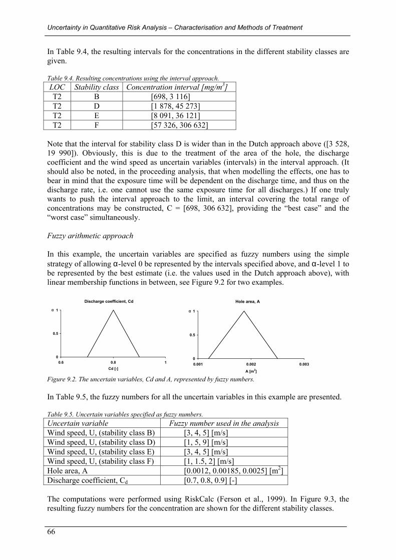
Uncertainty in Quantitative Risk Analysis – Characterisation and Methods of Treatment
66
In Table 9.4, the resulting intervals for the concentrations in the different stability classes are given. Table 9.4. Resulting concentrations using the interval approach. LOC Stability class Concentration interval [mg/m3] T2 B [698, 3 116] T2 D [1 878, 45 273] T2 E [8 091, 36 121] T2 F [57 326, 306 632]
Note that the interval for stability class D is wider than in the Dutch approach above ([3 528, 19 990]). Obviously, this is due to the treatment of the area of the hole, the discharge coefficient and the wind speed as uncertain variables (intervals) in the interval approach. (It should also be noted, in the proceeding analysis, that when modelling the effects, one has to bear in mind that the exposure time will be dependent on the discharge time, and thus on the discharge rate, i.e. one cannot use the same exposure time for all discharges.) If one truly wants to push the interval approach to the limit, an interval covering the total range of concentrations may be constructed, C = [698, 306 632], providing the “best case” and the “worst case” simultaneously. Fuzzy arithmetic approach In this example, the uncertain variables are specified as fuzzy numbers using the simple strategy of allowing α-level 0 be represented by the intervals specified above, and α-level 1 to be represented by the best estimate (i.e. the values used in the Dutch approach above), with linear membership functions in between, see Figure 9.2 for two examples.
Discharge coefficient, Cd
0
0.5
1
0.6 0.8 1Cd [-]
α
Hole area, A
0
0.5
1
0.001 0.002 0.003
A [m2]
α
Figure 9.2. The uncertain variables, Cd and A, represented by fuzzy numbers. In Table 9.5, the fuzzy numbers for all the uncertain variables in this example are presented. Table 9.5. Uncertain variables specified as fuzzy numbers. Uncertain variable Fuzzy number used in the analysis Wind speed, U, (stability class B) [3, 4, 5] [m/s] Wind speed, U, (stability class D) [1, 5, 9] [m/s] Wind speed, U, (stability class E) [3, 4, 5] [m/s] Wind speed, U, (stability class F) [1, 1.5, 2] [m/s] Hole area, A [0.0012, 0.00185, 0.0025] [m2] Discharge coefficient, Cd [0.7, 0.8, 0.9] [-] The computations were performed using RiskCalc (Ferson et al., 1999). In Figure 9.3, the resulting fuzzy numbers for the concentration are shown for the different stability classes.

Case study
67
Concentration, C, stability class B
0
0.5
1
500 1500 2500 3500
C [mg/m3]
α
Concentration, C, stability class D
0
0.5
1
0 25000 50000
C [mg/m3]
α
Concentration, C, stability class E
0
0.5
1
0 20000 40000
C [mg/m3]
α
Concentration, C, stability class F
0
0.5
1
50000 200000 350000
C [mg/m3]
α
Figure 9.3. Resulting fuzzy numbers for the concentration in the four stability classes. Not surprisingly, the range of the resulting concentration at α-level 0 is the same as for the interval analysis above, and the point estimation of the concentration at α-level 1 is the same as for the Dutch approach (apart from stability class D, where three different values of wind speed are used in the Dutch approach). However, the interpretation of the different α-levels is unfortunately not as clear-cut as one would like. At α-level 0, obviously the most conservative range is displayed, whereas at α-level 1 the most optimistic estimation is presented. The intermediate α-levels, however, can only be interpreted in very general terms, i.e. as α increases, the level of conservatism decreases. This reduces the practical use of this approach, in this specific example, to a fairly simple means of generating a “best case”, a “best estimate”, and a “worst case” in one single analysis. The fuzzy number approach will not be examined further in this example. Let us now turn to the probabilistic framework, where the interpretation of the distributions is much more straightforward. The Monte Carlo approach When using Monte Carlo procedures for uncertainty propagation, the uncertain variables must be specified as probability distributions. Here, the methods described in Chapter 5, or other standard statistical methods, may be used to construct the distribution based on the available information. In Table 9.6, the distributions used for the uncertain variables in this example are given.

Uncertainty in Quantitative Risk Analysis – Characterisation and Methods of Treatment
68
Table 9.6. Uncertain variables specified as probability distributions. Uncertain variable Distribution used in the analysis Wind speed, U, (stability class B) Normal (4, 0.4)11 [m/s] Wind speed, U, (stability class D) Normal (5, 1.5)[m/s] Wind speed, U, (stability class E) Normal (4, 0.4) [m/s] Wind speed, U, (stability class F) Uniform (1, 2)12 [m/s] Hole area, A Triang. (0.0012, 0.00187, 0.0025)13 [m2] Discharge coefficient, Cd Uniform (0.7, 0.9) [-] In the example, the Latin hypercube sampling scheme (10 000 iterations) was used for the sampling procedure. Independence between the uncertain variables was assumed. The calculations were performed using @risk from Palisade (2001). In Figure 9.4, the resulting probability distributions for the concentration in the different cases (i.e. stability classes) are shown. The distributions are given as complementary cumulative distribution functions, CCDFs. The interpretation of a CCDF is fairly simple. The y-axis represents the probability of the concentration, C, being ≥ c on the x-axis.
Concentration, C, stability class B
0
0.5
1
500 1500 2500 3500
c [mg/m3]
P(C
≥ c
)
Concentration, C, stability class D
0
0.5
1
0 25000 50000
c [mg/m3]
P (C
≥ c
)
Concentration, C, stability class E
0
0.5
1
0 20000 40000
c [mg/m3]
P(C
≥ c
)
Concentration, C, stability class F
0
0.5
1
50000 200000 350000
c [mg/m3]
P(C
≥ c
)
Figure 9.4. Resulting CCDFs for the concentration in the four stability classes. The above distributions are then used in the analysis as input for the calculation of effects. In situations where decisions are to be made using the concentration as a decision variable, the above distributions can be used directly, providing the possibility to choose a desired level of conservatism. For instance, a possible decision criterion could be that the probability of the concentration exceeding xx mg/m3 must not be higher than 5% (i.e. the 95% fractile of the
11 The notation ”Normal (4,0.4)” refers to a normal distribution with mean = 4, and standard deviation = 0.4. 12 The notation ”Uniform (1,2)” refers to a uniform distribution with minimum = 1, and maximum = 2. 13 The notation ”Triang. (0.0012, 0.00187, 0.0025)” refers to a triangular distribution with minimum = 0.0012, maximum = 0.0025, and mode = 0.00187.
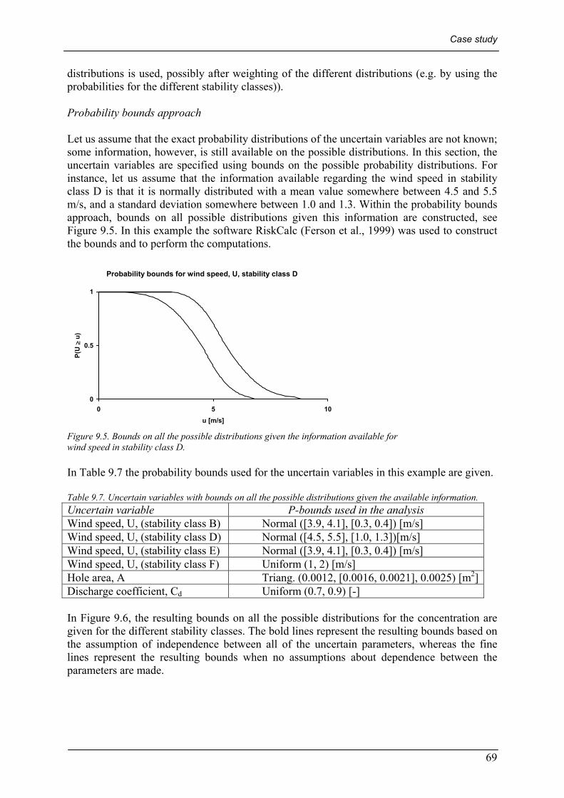
Case study
69
distributions is used, possibly after weighting of the different distributions (e.g. by using the probabilities for the different stability classes)). Probability bounds approach Let us assume that the exact probability distributions of the uncertain variables are not known; some information, however, is still available on the possible distributions. In this section, the uncertain variables are specified using bounds on the possible probability distributions. For instance, let us assume that the information available regarding the wind speed in stability class D is that it is normally distributed with a mean value somewhere between 4.5 and 5.5 m/s, and a standard deviation somewhere between 1.0 and 1.3. Within the probability bounds approach, bounds on all possible distributions given this information are constructed, see Figure 9.5. In this example the software RiskCalc (Ferson et al., 1999) was used to construct the bounds and to perform the computations.
Probability bounds for wind speed, U, stability class D
0
0.5
1
0 5 10u [m/s]
P(U
≥ u
)
Figure 9.5. Bounds on all the possible distributions given the information available for wind speed in stability class D. In Table 9.7 the probability bounds used for the uncertain variables in this example are given. Table 9.7. Uncertain variables with bounds on all the possible distributions given the available information. Uncertain variable P-bounds used in the analysis Wind speed, U, (stability class B) Normal ([3.9, 4.1], [0.3, 0.4]) [m/s] Wind speed, U, (stability class D) Normal ([4.5, 5.5], [1.0, 1.3])[m/s] Wind speed, U, (stability class E) Normal ([3.9, 4.1], [0.3, 0.4]) [m/s] Wind speed, U, (stability class F) Uniform (1, 2) [m/s] Hole area, A Triang. (0.0012, [0.0016, 0.0021], 0.0025) [m2] Discharge coefficient, Cd Uniform (0.7, 0.9) [-] In Figure 9.6, the resulting bounds on all the possible distributions for the concentration are given for the different stability classes. The bold lines represent the resulting bounds based on the assumption of independence between all of the uncertain parameters, whereas the fine lines represent the resulting bounds when no assumptions about dependence between the parameters are made.
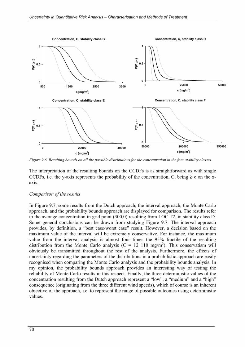
Uncertainty in Quantitative Risk Analysis – Characterisation and Methods of Treatment
70
Concentration, C, stability class B
0
0.5
1
500 1500 2500 3500
c [mg/m3]
P(C
≥ c
)
Concentration, C, stability class D
0
0.5
1
0 25000 50000
c [mg/m3]
P(C
≥ c
)
Concentration, C, stability class E
0
0.5
1
0 20000 40000
c [mg/m3]
P(C
≥ c
)
Concentration, C, stability class F
0
0.5
1
50000 200000 350000
c [mg/m3]
P(C
≥ c
)
Figure 9.6. Resulting bounds on all the possible distributions for the concentration in the four stability classes. The interpretation of the resulting bounds on the CCDFs is as straightforward as with single CCDFs, i.e. the y-axis represents the probability of the concentration, C, being ≥ c on the x-axis. Comparison of the results In Figure 9.7, some results from the Dutch approach, the interval approach, the Monte Carlo approach, and the probability bounds approach are displayed for comparison. The results refer to the average concentration in grid point (300,0) resulting from LOC T2, in stability class D. Some general conclusions can be drawn from studying Figure 9.7. The interval approach provides, by definition, a “best case/worst case” result. However, a decision based on the maximum value of the interval will be extremely conservative. For instance, the maximum value from the interval analysis is almost four times the 95% fractile of the resulting distribution from the Monte Carlo analysis (C = 12 110 mg/m3). This conservatism will obviously be transmitted throughout the rest of the analysis. Furthermore, the effects of uncertainty regarding the parameters of the distributions in a probabilistic approach are easily recognised when comparing the Monte Carlo analysis and the probability bounds analysis. In my opinion, the probability bounds approach provides an interesting way of testing the reliability of Monte Carlo results in this respect. Finally, the three deterministic values of the concentration resulting from the Dutch approach represent a “low”, a “medium” and a “high” consequence (originating from the three different wind speeds), which of course is an inherent objective of the approach, i.e. to represent the range of possible outcomes using deterministic values.
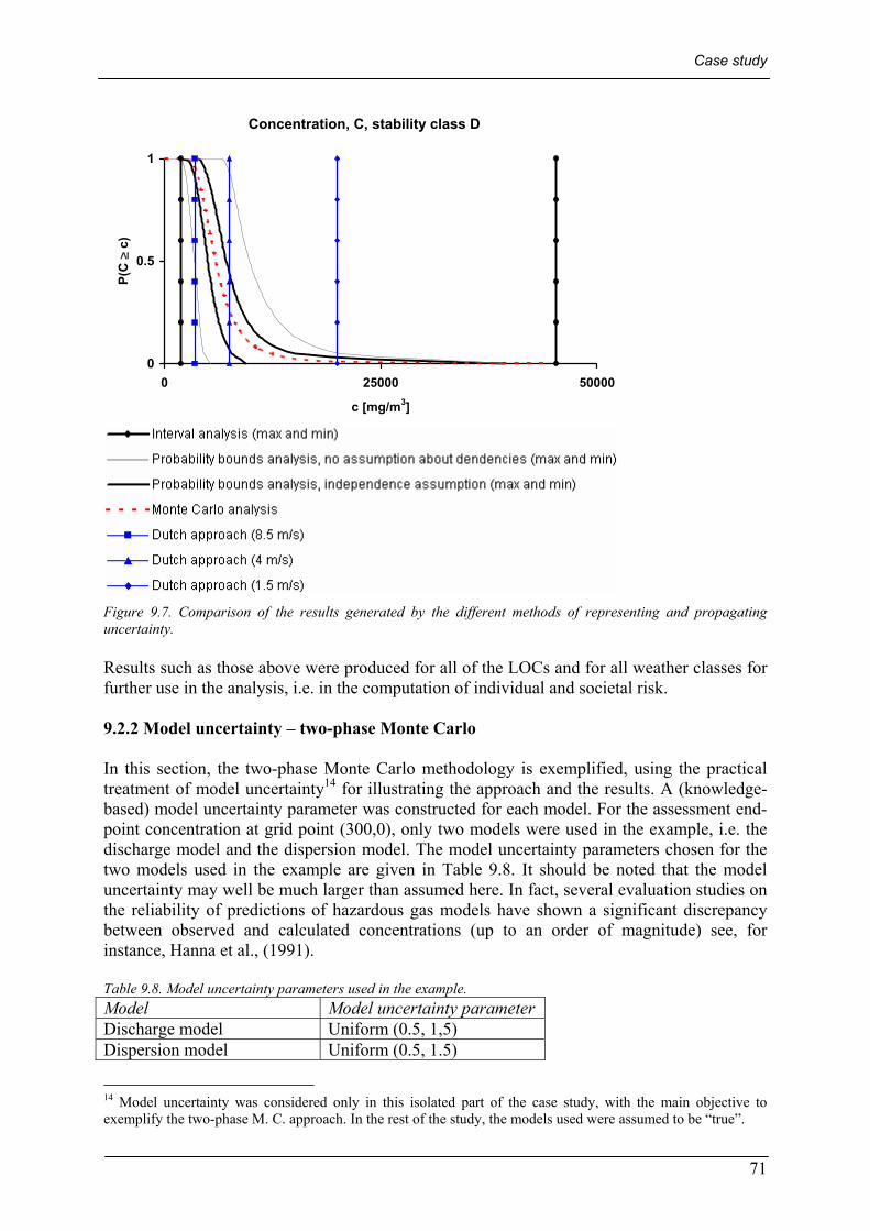
Case study
71
Concentration, C, stability class D
0
0.5
1
0 25000 50000
c [mg/m3]
P(C
≥ c
)
Figure 9.7. Comparison of the results generated by the different methods of representing and propagating uncertainty. Results such as those above were produced for all of the LOCs and for all weather classes for further use in the analysis, i.e. in the computation of individual and societal risk. 9.2.2 Model uncertainty – two-phase Monte Carlo In this section, the two-phase Monte Carlo methodology is exemplified, using the practical treatment of model uncertainty14 for illustrating the approach and the results. A (knowledge-based) model uncertainty parameter was constructed for each model. For the assessment end-point concentration at grid point (300,0), only two models were used in the example, i.e. the discharge model and the dispersion model. The model uncertainty parameters chosen for the two models used in the example are given in Table 9.8. It should be noted that the model uncertainty may well be much larger than assumed here. In fact, several evaluation studies on the reliability of predictions of hazardous gas models have shown a significant discrepancy between observed and calculated concentrations (up to an order of magnitude) see, for instance, Hanna et al., (1991). Table 9.8. Model uncertainty parameters used in the example. Model Model uncertainty parameter Discharge model Uniform (0.5, 1,5) Dispersion model Uniform (0.5, 1.5)
14 Model uncertainty was considered only in this isolated part of the case study, with the main objective to exemplify the two-phase M. C. approach. In the rest of the study, the models used were assumed to be “true”.

Uncertainty in Quantitative Risk Analysis – Characterisation and Methods of Treatment
72
In order to demonstrate one way of keeping different kinds of uncertainty separate in an analysis, a two-phase Monte Carlo procedure was performed, where the model uncertainty parameters were sampled in the outer loop, and all the other uncertain parameters were sampled in the inner loop. In Figure 9.8, the resulting CCDFs for the concentration at grid point (300,0) are presented, based on 40 cycles in the outer loop (and 10 000 iterations in the inner loop). The “dotted” CCDF is the result obtained from standard Monte Carlo analysis.
Concentration, C, stability class D
0
0.5
1
0 25000 50000
c [mg(m3]
P(C
≥ c
)
Figure 9.8. Resulting CCDFs from the two-phase Monte Carlo procedure. As stated earlier, the spread of distributions is due to model uncertainty, whereas each CCDF represents the uncertainty in all the other parameters. This methodology can of course be applied to whichever uncertain parameters the analyst wants to treat separately in an analysis. The most common use of this methodology is to separate stochastic and knowledge-based uncertainty.
9.3 Individual risk at grid point (300,0) For the calculation of individual risk at grid point (300,0), the general procedure described in CCPS (2000) was followed. Based on the distributions (and intervals/point estimates) of the concentration at grid point (300,0), the probit equation was used to produce distributions of the probability of death at grid point (300,0). Furthermore, the frequency of the different LOCs was estimated, together with probabilities for different stability classes, wind directions, etc, see Appendix 3. The procedure of calculating the individual risk can also be found in Appendix 3, in the description of an example RiskCalc file, together with an overview of all the uncertain variables in the example, and how the uncertainty was specified within the different approaches. In Figure 9.9, the resulting individual risk estimates at grid point (300,0), generated by the different methods, are displayed. The Dutch (standard QRA) approach generates a point estimate of the individual risk, while the different methods of uncertainty analysis provide a range or distribution of the individual risk, thus accounting for the various uncertainties in the calculations.
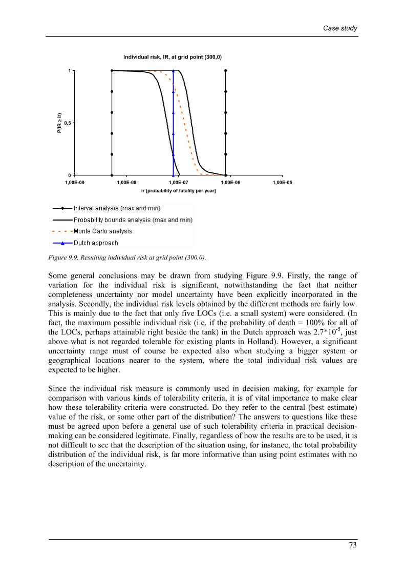
Case study
73
Individual risk, IR, at grid point (300,0)
0
0,5
1
1,00E-09 1,00E-08 1,00E-07 1,00E-06 1,00E-05ir [probability of fatality per year]
P(IR
≥ ir
)
Figure 9.9. Resulting individual risk at grid point (300,0). Some general conclusions may be drawn from studying Figure 9.9. Firstly, the range of variation for the individual risk is significant, notwithstanding the fact that neither completeness uncertainty nor model uncertainty have been explicitly incorporated in the analysis. Secondly, the individual risk levels obtained by the different methods are fairly low. This is mainly due to the fact that only five LOCs (i.e. a small system) were considered. (In fact, the maximum possible individual risk (i.e. if the probability of death = 100% for all of the LOCs, perhaps attainable right beside the tank) in the Dutch approach was 2.7*10-5, just above what is not regarded tolerable for existing plants in Holland). However, a significant uncertainty range must of course be expected also when studying a bigger system or geographical locations nearer to the system, where the total individual risk values are expected to be higher. Since the individual risk measure is commonly used in decision making, for example for comparison with various kinds of tolerability criteria, it is of vital importance to make clear how these tolerability criteria were constructed. Do they refer to the central (best estimate) value of the risk, or some other part of the distribution? The answers to questions like these must be agreed upon before a general use of such tolerability criteria in practical decision-making can be considered legitimate. Finally, regardless of how the results are to be used, it is not difficult to see that the description of the situation using, for instance, the total probability distribution of the individual risk, is far more informative than using point estimates with no description of the uncertainty.
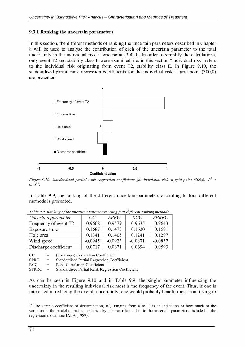
Uncertainty in Quantitative Risk Analysis – Characterisation and Methods of Treatment
74
9.3.1 Ranking the uncertain parameters In this section, the different methods of ranking the uncertain parameters described in Chapter 8 will be used to analyse the contribution of each of the uncertain parameter to the total uncertainty in the individual risk at grid point (300,0). In order to simplify the calculations, only event T2 and stability class E were examined, i.e. in this section “individual risk” refers to the individual risk originating from event T2, stability class E. In Figure 9.10, the standardised partial rank regression coefficients for the individual risk at grid point (300,0) are presented.
-1 -0.5 0 0.5 1
1
Coefficient value
Frequency of event T2
Exposure time
Hole area
Wind speed
Discharge coefficient
Figure 9.10. Standardised partial rank regression coefficients for individual risk at grid point (300,0). R2 ≈ 0.9815. In Table 9.9, the ranking of the different uncertain parameters according to four different methods is presented. Table 9.9. Ranking of the uncertain parameters using four different ranking methods. Uncertain parameter CC SPRC RCC SPRRC Frequency of event T2 -0.9608 -0.9579 -0.9635 -0.9643 Exposure time -0.1687 -0.1473 -0.1630 -0.1591 Hole area -0.1341 -0.1405 -0.1241 -0.1297 Wind speed -0.0945 -0.0923 -0.0871 -0.0857 Discharge coefficient -0.0717 -0.0671 -0.0694 -0.0593
CC = (Spearman) Correlation Coefficient SPRC = Standardised Partial Regression Coefficient RCC = Rank Correlation Coefficient SPRRC = Standardised Partial Rank Regression Coefficient As can be seen in Figure 9.10 and in Table 9.9, the single parameter influencing the uncertainty in the resulting individual risk most is the frequency of the event. Thus, if one is interested in reducing the overall uncertainty, one would probably benefit most from trying to
15 The sample coefficient of determination, R2, (ranging from 0 to 1) is an indication of how much of the variation in the model output is explained by a linear relationship to the uncertain parameters included in the regression model, see IAEA (1989).
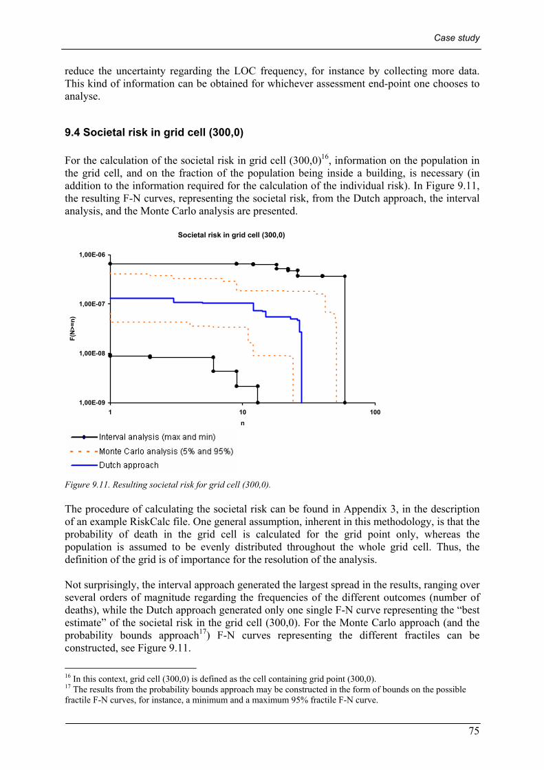
Case study
75
reduce the uncertainty regarding the LOC frequency, for instance by collecting more data. This kind of information can be obtained for whichever assessment end-point one chooses to analyse.
9.4 Societal risk in grid cell (300,0) For the calculation of the societal risk in grid cell (300,0)16, information on the population in the grid cell, and on the fraction of the population being inside a building, is necessary (in addition to the information required for the calculation of the individual risk). In Figure 9.11, the resulting F-N curves, representing the societal risk, from the Dutch approach, the interval analysis, and the Monte Carlo analysis are presented.
Societal risk in grid cell (300,0)
1,00E-09
1,00E-08
1,00E-07
1,00E-06
1 10 100n
F(N
>=n)
Figure 9.11. Resulting societal risk for grid cell (300,0). The procedure of calculating the societal risk can be found in Appendix 3, in the description of an example RiskCalc file. One general assumption, inherent in this methodology, is that the probability of death in the grid cell is calculated for the grid point only, whereas the population is assumed to be evenly distributed throughout the whole grid cell. Thus, the definition of the grid is of importance for the resolution of the analysis. Not surprisingly, the interval approach generated the largest spread in the results, ranging over several orders of magnitude regarding the frequencies of the different outcomes (number of deaths), while the Dutch approach generated only one single F-N curve representing the “best estimate” of the societal risk in the grid cell (300,0). For the Monte Carlo approach (and the probability bounds approach17) F-N curves representing the different fractiles can be constructed, see Figure 9.11.
16 In this context, grid cell (300,0) is defined as the cell containing grid point (300,0). 17 The results from the probability bounds approach may be constructed in the form of bounds on the possible fractile F-N curves, for instance, a minimum and a maximum 95% fractile F-N curve.
Uncertainty in Quantitative Risk Analysis – Characterisation and Methods of Treatment
76
Obviously, if one is interested in the total societal risk a plant poses to its surroundings, one would have to calculate the contributions from all the grid cells that are within the effect zone of the plant, and then construct the total F-N curve(s) based on this information. The same discussion as for the individual risk applies to societal risk regarding comparison of the results with absolute tolerability criteria.
9.5 Conclusions from the case study First and foremost, it has been shown that methods are available for representing and treating uncertainty which makes it possible to account for different types of uncertainty in all stages of an analysis. Furthermore, methods are available for identifying which parameters in the risk analysis model affect the final uncertainty in the results to the highest degree, thus making it possible to direct efforts in reducing the total uncertainty, should it prove necessary. However, the calculations rapidly become complex and extensive when a full analysis of the uncertainty, for instance using the Monte Carlo method, is to be performed. Regarding the different methods of uncertainty propagation used in the example, some general conclusions may be drawn. The interval approach provides a fairly straightforward way of performing a “best case/worst case” analysis simultaneously. The fuzzy number approach provides little extra value due to the problems associated with interpretation of the different α-levels. Probabilistic (Monte Carlo) analysis provides the most versatile approach, mainly due to the possibility of keeping different types of uncertainty separate during an analysis and its strong theoretical foundations. The probability bounds approach provides an interesting method for primarily quality assurance for Monte Carlo analyses. Furthermore, the range of variation for the resulting risk in the example is significant, notwithstanding the fact that neither completeness uncertainty nor model uncertainty have been explicitly incorporated in the analysis. The implications such an uncertainty range may have on the applicability of target risks (tolerability criteria) are apparent. Finally, it can once again be stressed that performing a full uncertainty analysis is inherently time-consuming. The importance of finding ways of differentiating levels of treatment of uncertainty is clear.

Conclusions and recommendations
77
10. Conclusions and recommendations
10.1 Conclusions drawn from the study In this section some general conclusions drawn from the study will be presented, followed by a number of recommendations regarding future work and research in this area. In Sweden, it is possible to discern a substantial increase in the use of quantitative risk analysis as part of the basis for decision making regarding safety-related issues in various areas, for instance land use planning, licensing procedures for hazardous activities, and infrastructure projects. The QRA methodology has proven to be of considerable use regarding the determination of major contributions to risk, and for the evaluation of different decision options with respect to risk. However, due to a lack of consensus concerning which methods, models and inputs should be used in an analysis, and how the uncertainties that will inevitably be introduced during the process should be handled, questions arise regarding the credibility and usefulness of the absolute results from QRA. The results of a European benchmark study regarding the impact of uncertainties on the results of quantitative risk analyses, in which several teams were asked to perform an analysis of the same facility, showed a very large variation between the different teams, originating from different methods, models and basic assumptions. The problems related to such variation are of greatest concern in situations where the quantitative (absolute) estimation of the risk is to be evaluated regarding tolerability. Without a description and discussion of the uncertainties involved in such an analysis, the practical use of the results in absolute terms will be questionable. For example, comparison of the results with established risk targets, or tolerability criteria, becomes a fairly arbitrary exercise. In this dissertation, a variety of methods of identifying, quantifying and analysing uncertainties within the QRA framework has been presented and discussed, together with discussions on model reliability and various structured procedures of eliciting information from experts. It is concluded that methods exist for dealing with most kinds of uncertainty, with sufficient sophistication for most problems introduced by those uncertainties in practical decision-making situations. The presentation given may serve as a basis for discussions in future work on standardisation regarding quantitative risk analysis in different sectors of industry. A general conclusion, with respect to future standardisation, is that the probabilistic framework appears to be the most promising for treatment of uncertainties in such analyses. This is due to its strong theoretical foundations and the possibility of quantifying, and analysing, uncertainties originating from fundamentally different sources (e.g. aleatory and epistemic uncertainty) separately. The treatment of knowledge-based uncertainty within the probabilistic framework implies probability being regarded as a degree of belief, i.e. the Bayesian point of view. Some types of uncertainty, however, mainly related to questions of completeness and general quality issues, are intrinsically problematic (and challenging) when it comes to rational ways of quantification and analysis. For instance, the explicit inclusion of organisational factors in the QRA is an area that needs to be developed further. Some attempts at dealing with this problem have been examined within this study, and it is concluded that this is still an area under rapid development.
Uncertainty in Quantitative Risk Analysis – Characterisation and Methods of Treatment
78
Another question of major concern in this study was the level of uncertainty description and analysis required in different situations. Obviously, due to differences regarding, for instance, problem complexity and the nature of the hazard source, different levels of uncertainty analysis might be called for in order to make the analysis useful in practical decision-making situations. In this dissertation, a discussion on arguments for and against the different methods of uncertainty analysis is presented, together with a discussion on different levels of treatment, which might serve as a basis for further debate on how to differentiate the requirements of uncertainty treatment, based on the situation under consideration, in future guidelines for quantitative risk analysis.
10.2 Recommendations on future research and standardisation efforts In order to make the results of quantitative risk analyses useful in practical decision situations, efforts must be made to ensure that such results are verifiable, reproducible and comparable. To be able to reach this goal, some recommendations on the subject of future research and standardisation are presented below. Possible ways of standardising the QRA process at a national level should be assessed. However, generic guidelines across all sectors of industry are not deemed viable, due to the different conditions under which they operate. Instead, differences between industrial sectors, for instance, the chemical process industry and the transportation industry, would have to be acknowledged in such work, presumably resulting in separate guidelines. A possible starting point for such work would be to examine the Dutch guidelines presented in the report from the Committee for the Prevention of Disasters (1999). Below, some key elements of such future standardisation efforts are highlighted.
• While undertaking preparatory work for such guidelines, emphasis must be placed on the treatment of uncertainties introduced in an analysis. This report may serve as a basis for discussions regarding these issues, especially the quantification and treatment of parameter uncertainty.
• Efforts must be made to assess how questions of general quality and completeness
uncertainty are to be handled within an analysis. Some attempts at dealing with this problem have been discussed in this dissertation. Consensus on methods of quantifying or, in some other way, dealing this type of uncertainty must be reached.
• Possible ways of differentiating the level of uncertainty description and analysis
required, based on the situation under consideration, should be examined within each sector of industry. The discussion presented in this dissertation on various levels of treatment may serve as a basis for further debate.
• As stated above, differences between different sectors of industry call for separate
guidelines. A natural starting point for future standardisation efforts would be to consider the risk analysis process for industrial sites that are required to produce a safety report according to the European Council Directive (96/82/EC), the “Seveso II Directive”. This is partly due to the relatively well-defined problems related to such sites, and also due to the fact that risk analysis is routinely performed for such establishments.

Conclusions and recommendations
79
• This kind of work is an absolute necessity for the general use of risk tolerability criteria to be meaningful.
It is my firm belief that such work would facilitate many of the situations where decision-makers today are struggling to find a solid foundation on which to make robust decisions regarding risk-related issues.

Uncertainty in Quantitative Risk Analysis – Characterisation and Methods of Treatment
80

Acknowledgements
81
Acknowledgements I would like to express my sincere gratitude to my supervisor, Professor Sven Erik Magnusson, for his encouragement and patience during the process which resulted in this dissertation. Many thanks are also directed towards Mr Robert Jönsson and all my colleagues at the Department of Fire Safety Engineering, Lund University. The financial support of the work on which this dissertation is based, provided by the Swedish Rescue Services Agency, is gratefully acknowledged. This work is part of a project entitled Behandling av osäkerheter i kvantitativa riskanalyser (The Treatment of Uncertainties in Quantitative Risk Analyses). Finally, to my wife and dear friend Sofie, you deserve my very special thanks for your continuous love and support. You really make all the difference…

Uncertainty in Quantitative Risk Analysis – Characterisation and Methods of Treatment
82

References
83
References
Databases MHIDAS (Major Hazard Incident Data Service) http://www.hse.gov.uk/infoserv/mhidas.htm (2001-05-30). FACTS (Failure and Accident Technical Information System) http://www.mep.tno.nl (2001-05-30). The Accident Database, IchemE, http://www.environment97.org/framed/icheme/ichememain5.htm (2001-05-30). MARS (Major Accident Reporting System) http://mahbsrv.jrc.it/Activities-WhatIsMARS.html (2001-05-30). OREDA Offshore Reliability Data Handbook, third edition, http://www.sintef.no/sipaa/prosjekt/oreda/handbook.html (2001-05-30). Guidelines for Process Equipment Reliability Data – with Data Tables, Center for Chemical Process Safety, American Institute of Chemical Engineers, New York, 1989.
General References Abrahamsson, M., Treatment of Uncertainty in Risk Based Regulations and Standards for Risk Analysis. Report 3116, Department of Fire Safety Engineering, Lund University, Lund, 2000. Abrahamsson, M., Behandling av osäkerheter i riskanalyser – Studie av befintliga analyser. Department of Fire Safety Engineering, Lund University, Lund, to be published. (In Swedish). Abrahamsson, M., Johansson, H., & Magnusson, S.E., Methods for treatment of uncertainty in quantitative risk analysis. Safety, Risk and Reliability – Trends in Engineering, Conference report, IABSE, Zürich, 2001. Abrahamsson, M., & Magnusson, S.E., Treatment of uncertainties in quantitative risk analysis. Foresight and Precaution, Cottham, Harvey, Pape & Tait (eds.), Balkema, Rotterdam, 2000. Alefeld, G., & Herzberger, J., Introduction to Interval Computations. Academic Press, New York, 1983. Amendola, A., Contini, S., & Ziomas, I., Uncertainties in chemical risk assessment: Results of a European benchmark exercise. Journal of Hazardous Materials, vol. 29, Elsevier Science Publishers, Amsterdam, 1992.

Uncertainty in Quantitative Risk Analysis – Characterisation and Methods of Treatment
84
Ang, A.H-S., & Tang, W.H., Probability concepts in Engineering Planning and Design, Volume 1 – Basic Principles. John Wiley & Sons, New York, 1975. CCPS, Guidelines for Chemical Process Quantitative Risk Analysis. Center for Chemical Process Safety, American Institute of Chemical Engineers, New York, 2000. Clemen R.T., Making Hard Decisions – An Introduction to Decision Analysis. Wadsworth Publishing Company, Belmont, 1996. Committee for the Prevention of Disasters, Guidelines for Quantitative Risk Assessment. CPR18E “Purple book”. Sdu Uitgevers, Den Haag, 1999. Cooke R.M., Experts in Uncertainty – Opinion and Subjective Probability in Science. Oxford University Press, New York, 1991. COWI, Usikkerhedsbeskrivelse i kvantitative risikoanalyser – vejledning. COWI, Denmark, 1996a. (In Danish). COWI, Usikkerhedsbeskrivelse i kvantitative risikoanalyser – projektrapport. COWI, Denmark, 1996b. (In Danish). COWI, Usikkerhedsbeskrivelse i kvantitative risikoanalyser – gasspredningsmodeller. COWI, Denmark, 1996c. (In Danish). COWI, Usikkerhedsbeskrivelse i kvantitative risikoanalyser – litteraturgennemgang. COWI, Denmark, 1996d. (In Danish). Dwyer, P., Linear Computations. John Wiley & Sons, New York, 1951. Davidsson, G., Haeffler, L., Hannah, J., & Akersten, P.A., Databaser om olyckor och olycksrisker. Räddningsverket, Karlstad, 1999. (In Swedish). Davidsson, G., Lindgren, M., & Mett, L., Värdering av risk. Räddningsverket, Karlstad, 1997. (In Swedish). Ferson, S., & Kuhn, R., Propagating uncertainty in ecological risk analysis using interval and fuzzy arithmetic. Computer Techniques in Environmental Studies IV, Elsevier Applied Science, London, 1992. Ferson, S., & Ginzburg, L.R., Different methods are needed to propagate ignorance and variability. Reliability Engineering and System Safety 54, Elsevier Science limited, Northern Ireland, 1996. Ferson, S., & Sunil, D., Probability Bounds Analysis. Proceedings of the 4th International Conference on Probabilistic Safety Assessment and Management, PSAM 4, Edited by Mosleh, A. & Bari, R.A., New York, 1998. Ferson, S., Root, W., & Kuhn, R., Ramas Risk Calc – Risk Assessment with Uncertain Numbers. Applied Biomathematics, Setauket, New York, 1999.
References
85
Fisher, S., Forsén, R., Hertzberg, O., Jacobsson, A., Koch, B., Runn, P., Thaning, L., & Winter, S., Vådautsläpp av brandfarliga och giftiga gaser och vätskor – metoder för bedömning av risker. Försvarets Forskningsanstalt, Grindsjön, 1997. (In Swedish). Frantzich, H., Uncertainty and Risk Analysis in Fire Safety Engineering. Doctoral dissertation, Department of Fire Safety Engineering, Lund University, Lund, 1998. Frantzich, H., Harrada, K., & Magnusson S.E., Fire Safety Design Based on Calculations – Uncertainty Analysis and Safety Verification. Report 3078, Department of Fire Safety Engineering, Lund University, Lund, 1995. Furuta, H., & Shiraishi, N., Fuzzy importance in fault tree analysis. Fuzzy Sets and Systems 12, Elsevier Science, 1984. Hale, A.R., & Hovden, J. Management and Culture: the third age of safety. Occupational Injury: Risk, Prevention and Intervention, Edited by Feyer, A.M., and Williamson A. Taylor & Francis, United Kingdom, 1998. Hale, A.R., Oh, J.I.H., Brouwer, W.G.J., Bellamy, L.J., Ale, B.J.M., & Papazoglou, I.A. The IRISK project: Development of an integrated technical and management risk control and monitoring methodology for managing and quantifying on-site and off-site risks. Proceedings of the 4th International Conference on Probabilistic Safety Assessment and Management, PSAM 4, Edited by Mosleh, A., & Bari R.A., New York, 1998a. Hanna, S.R., Strimaitis, D.G., & Chang, J.C., Evaluation of fourteen hazardous gas models with ammonia and hydrogen fluoride field data. Elsevier Science Publishers, Amsterdam, 1991. Hendershot, D.C., Risk Guidelines as a Risk Management Tool. Prepared for presentation at the 1996 Process Plant Safety Symposium. Rohm and Haas Company, Bristol, 1995. Helton, J.C., & Davis, F.J. Sampling-Based Methods for Uncertainty and Sensitivity Analysis. Sandia Report SAND99-2240, Sandia National Laboratories, Albuquerque, 2000. Hofer, E., When to Separate Uncertainties and When Not to Separate. Reliability Engineering and System Safety 54, Elsevier Science limited, Northern Ireland, 1996. IAEA, Evaluating the reliability of predictions made using environmental transfer models. International Atomic Energy Agency, Vienna, 1989. IEC, International standard nr 60300-3-9: Dependability management – part 3: Application guide – Section 9: Risk analysis of technological systems. International Electrotechnical Commision, Geneva, 1995. Iman, R.L., Davenport, J.M., & Ziegler, D.K., Latin Hypercube sampling (a program user’s guide). Technical Report SAND79-1473, Sandia National Laboratories, Albuquerque, 1980. Iman, R.L. & Helton, J.C., An Investigation of Uncertainty and Sensitivity Analysis Techniques for Computer Models. Risk Analysis 8, no. 1, Kluwer Academic/Plenum Publishers, New York, 1988.
Uncertainty in Quantitative Risk Analysis – Characterisation and Methods of Treatment
86
Isukapalli, S.S., Uncertainty analysis of transport-transformation models. PhD dissertation, The State University of New Jersey, New Brunswick, 1999. Johnson, N.L., Kotz, K., & Kemp, A.D., Univariate Discrete distributions. John Wiley & Sons, New York, 1993. Johnson, N.L., Kotz, K., & Balakrishnan, N., Continuous Univariate distributions (Vol. 1). John Wiley & Sons, New York, 1994. Johnson, N.L., Kotz, K., & Balakrishnan, N., Continuous Univariate distributions (Vol. 2). John Wiley & Sons, New York, 1995. Kahneman, D., Slovic, P., & Tversky, A., (eds.) Judgement under Uncertainty, Heuristics and Biases. Cambridge University Press, Cambridge, 1982. Kaufmann, A., & Gupta, M.M., Introduction to Fuzzy Arithmetic – Theory and Applications. Van Nostrand Reinhold, New York, 1985. Laskey, K., Model confidence (Lecture notes) Summer Institute on Probability in AI, George Mason University, 1994. Lauridsen, K., Christou, M., Amendola, A., Markert, F., Kozine, I., & Fiori, M., Assessing the Uncertainties in the Process of Risk Analysis of Chemical Establishments: Part 1. Proceedings ESREL conference Towards a Safer World, Torino, 2001a. Available from: http://www.aidic.it/italiano/congressi/esrel2001/webpapersesrel2001/pro.html (2002-02-05) Lauridsen, K., Christou, M., Amendola, A., Markert, F., Kozine, I., & Fiori, M., Assessing the Uncertainties in the Process of Risk Analysis of Chemical Establishments: Part 2. Proceedings ESREL conference Towards a Safer World, Torino, 2001b. Available from: http://www.aidic.it/italiano/congressi/esrel2001/webpapersesrel2001/pro.html (2002-02-05) Lees, F.P., Loss Prevention in the Process Industries. 2:nd edition, Vol. 1-3, Butterworth-Heinemann, Oxford, 1996. Model Evaluation Group, Model Evaluation Protocol. Can be requested from the European Communities, DG XII/D1, Rue de la Loi 200, B-1049 Brussels, Belgium, 1994. Moore, R.E. Methods and Applications of Interval Analysis. SIAM Studies on Applied Mathematics, Vol. 2, Philadelphia, 1979. Moore, R.E., Interval analysis. Prentice-Hall, Englewood Cliffs, New Jersey, 1966. Morgan, G.M., & Henrion, M., Uncertainty – A guide to Dealing with Uncertainty in Quantitative Risk and Policy Analysis. Cambridge University Press, New York, 1990.

References
87
Murphy, D.M., & Paté-Cornell, E., The SAM Framework: Modelling the Effects of Management Factors on Human Behaviour in Risk Analysis. Risk Analysis, Vol. 16, No 4, Plenum Press, New York, 1996. Olesen, H.R., Ten years of Harmonisation activities: Past, present and future. Introductory address to the 7th International conference on Harmonisation within Atmospheric Dispersion Modelling for Regulatory Purposes, Belgirate, Italy, May 2001. Proceedings available from: http://www.dmu.dk/atmosphericenvironment/Harmoni/ProcIntr.htm (2002-02-05) Palisade Corporation, Guide to using @RISK. Palisade Corporation, Newfield, 2001. Parry, G.W., Uncertainty in PRA and its Implications for use in Risk-Informed Decision Making. Proceedings of the 4th International Conference on Probabilistic Safety Assessment and Management, PSAM 4, Edited by Mosleh, A. & Bari, R.A., New York, 1998. Paté-Cornell, M.E., Uncertainty in risk analysis: Six levels of treatment. Reliability Engineering and System Safety 54, Elsevier Science limited, Northern Ireland, 1996. Paté-Cornell, M.E., Priorities in Risk Management: Human and Organisational Factors as External Events and a Maritime Illustration. Proceedings of the 4th International Conference on Probabilistic Safety Assessment and Management, PSAM 4, Edited by Mosleh, A. & Bari, R.A., New York, 1998. Rasmussen, J., Risk Management, Adaptation, and Design for Safety. In Sahlin, N.E., and Brehmer, B., (Eds.) Future Risks and Risk Management, Kluwer, Dordrecht, 1994. Rasmussen, J., Risk Management in a Dynamic Society: A Modelling Problem. In Safety Science 27/2-3, pp 183-213, Elsevier Science, 1997. Robinson, D.G., A Survey of Probabilistic Methods Used in Reliability, Risk and Uncertainty Analysis: Analytical Techniques 1. Sandia Report SAND98-1189, Sandia National Laboratories, Albuquerque, 1998. Saccomanno, F.F., & Bakir, O., Analysis of Risk Uncertainty for the Transport of Hazardous Materials. In Transportation of Dangerous Goods: Assessing the Risks. Institute for Risk Research, University of Waterloo, Ontario, Canada, 1991. Saltelli, A., & Sobol, I.M., About the Use of Rank Transformation in Sensitivity Analysis of Model Output. In Reliability Engineering and System Safety, Vol. 50, no. 3. Elsevier Science limited, Northern Ireland 1995 Schemel, S.D., Schemel, C.F., & Van Brunt, V., Methodology for determining reliability of a foam suppression system using fuzzy set theory and fault tree analysis. Appendix A in “Aircraft Hangar Fire Suppression System Design Study”. Scheffey et al., Naval Research Laboratory, Washington DC, 2000. Sklet, S., & Øien, K., Bruk av risikoanalyser i driftsfasen, etablering av sikkerhetsindikatorer og modellering av organisatoriske faktorers effekt på risikonivået – en ”state of the art” beskrivelse. SINTEF rapportnr. STF38 A99416, SINTEF, Trondheim, 1999. (In Norwegian).

Uncertainty in Quantitative Risk Analysis – Characterisation and Methods of Treatment
88
Slovic, P., Fischoff, B., & Lichtenstein, S., Facts versus Fears: Understanding Perceived Risk. In Kahneman, D., Slovic, P., and Tversky, A., (eds.) Judgement under Uncertainty, Heuristics and Biases. Cambridge University Press, Cambridge, 1982. Stirling, A., Renn, O., Klinke, A., Rip, A., & Salo, A., On Science and Precaution in the Management of Technological Risk. EUR 19056 EN, ECSC-EEC-EAEC, Luxembourg, 1999. Suresh, P.V., Babar, A.K., & Venkat Raj, V., “Uncertainty in fault tree analysis: A fuzzy approach. Fuzzy Sets and Systems 83, Elsevier Science, 1996. Tversky, A., & Kahneman, D., Availability: A Heuristic for Judging Frequency and Probability. In Kahneman, D., Slovic, P., and Tversky, A., (eds.) Judgement under Uncertainty, Heuristics and Biases, Cambridge University Press, Cambridge, 1982a. Tversky, A., & Kahneman, D., Causal Schemas in Judgements Under Uncertainty. In Kahneman, D., Slovic, P., and Tversky, A., (eds.) Judgement under Uncertainty, Heuristics and Biases, Cambridge University Press, Cambridge, 1982b. Tversky, A., & Kahneman, D., Judgement under Uncertainty: Heuristics and Biases. In Kahneman, D., Slovic, P., and Tversky, A., (eds.) Judgement under Uncertainty, Heuristics and Biases, Cambridge University Press, Cambridge, 1982c. U.S. Environmental Protection Agency, Policy for use of Probabilistic Analysis in Risk Assessment and Guiding Principles for Monte Carlo Analysis. EPA/630/R-97/001, EPA, 1997. Vose, D., Risk Analysis – A Quantitative Guide. 2:nd edition. John Wiley & Sons Ltd., Chichester, 2000. Winkler, R.L., Uncertainty in Probabilistic Risk Assessment. Reliability Engineering and System Safety 54, Elsevier Science limited, Northern Ireland, 1996. Zadeh, L.A., Fuzzy sets. Information and Control Theory 8:338-353, 1965.
Appendix 1
89
Appendices
APPENDIX 1 Examples of existing databases This appendix contains short, non-exhaustive descriptions of some databases relevant to risk analysis, with emphasis on describing the kind of information available in each of them. A.1.1 Accident (event) databases MHIDAS (Major Hazard Incident Data Service) The Major Hazard Incidents Data Service (MHIDAS) is maintained by AEA Technology by appointment of HSE (Health & Safety Executive, Great Britain). The database contains approximately 7000 incidents where dangerous substances were released and affected, or could have affected the surroundings, in the process industry, during transportation or during storage. This definition contains events that lead to casualties, evacuation and/or effect on the environment or property. Events that under a different set of conditions could have lead to any of the above are also included in the database. Some special kinds of incidents, such as incidents including radioactive materials, have been omitted from the database. All information in the MHIDAS is collected from publicly available sources of information, including approximately 30 technical/scientific journals, and information from the company involved in the event. Most of the approximately 7000 events are collected from either Great Britain or the United States of America. The database contains information from 1964 and onwards and is updated quarterly. Events are not included in the database until one year after they take place. The reason for this is that efforts are made to ensure maximum coverage of the event, e.g. by using multiple sources of information. There are several ways to get access to the MHIDAS database, none of which are for free. An adapted service is available from AEA Technology. The database is also available on OSH-ROM through SilverPLatter InformationLtd, or as an Internet service through European Information Network Services (EINS) FACTS (Failure and Accident Technical Information System) Failure and Accident Technical Information System (FACTS) is maintained by the Dutch research organisation TNO. The database has been in use since 1980 and contains information about approximately 16 000 industrial accidents and incidents from 1900 - today. Approximately 700 new events are added every year and about 500 existing events are updated when new information becomes available. The information in the FACTS database is collected via, for instance, symposium proceedings, periodic journals with focus on industrial safety, risk management and loss prevention. Other important sources are companies (supplies data with the proviso that strict anonymity applies), authorities, organisations with internal report systems, e.g. the rescue services (supplies data with the proviso that strict anonymity applies) etc. The database contains no population-, components- or operational data that can be used to estimate failure frequencies. The FACTS database is available through TNO, Division of Technology for Society, either on diskettes, CD-ROM or in paper format.

Uncertainty in Quantitative Risk Analysis – Characterisation and Methods of Treatment
90
The Accident Database The Accident Database is maintained by the Institute of Chemical Engineers (IchemE). The database contains more than 8000 accidents and incidents. All information in the database is based on information provided by companies dealing with dangerous substances or processes. Approximately 3000 events are based on internal company reports that have not been publicly available before. The Accident Database is available on CD-ROM from IchemE. MARS (Major Accident Reporting System) Most of the information about MARS presented here is taken from the MAHB (Major Accident Hazards Bureau) web-page: http://mahbsrv.jrc.it/Activities-WhatIsMARS.html (where more information is available). The Major Accident Reporting System (MARS) was established to handle the information on major accidents submitted by Member States of the European Union to the European Commission in accordance with the provisions of the Seveso Directive. Currently, MARS holds data on more than 450 major accidents. Two reporting forms have been established. The “short report” is intended for use for immediate notification of an accident, and the "full report" is prepared when the accident has been fully investigated, and the causes, the evolution of the accident, and the consequences are fully understood. In certain cases further information comes to light - for example in the course of judicial proceedings - and there is provision for the 'full report' information to be further modified. The “short report” gives essential information concerning the accident, in a free-text format, under the following headings:
• Accident type • Substances directly involved • Immediate sources of accident • Immediate causes • Immediate effects • Emergency measures taken • Immediate lessons learnt
The “full report” is much more analytic, and involves more work in its preparation. While there are always “free-text” fields available to describe facts connected with an accident, substantial effort has been put into the definition of descriptive codes, for the accident itself and for associated information, to enable the MARS database to be searched under almost 200 different headings (data variables), e.g.:
Appendix 1
91
• Type of accident • Industry where accident occurred • Activity being carried out • Components directly involved • Causative factors (immediate and underlying) • Ecological systems affected • Emergency measures taken
This information is then used to perform lessons-learnt type of data analyses, identifying significant dependencies and overall patterns in the data. A.1.2 Failure frequency databases The accident (event) databases briefly presented above focuses on describing possible causes and the general course of events leading to accidents or near accidents. In addition to this kind of documentation of accident scenarios, failure frequency databases contains information and data which makes it possible to calculate different kinds of reliability measures, e.g. failure probabilities (frequencies) of components. OREDA OREDA – Offshore Reliability Data is a collaboration project among several enterprises (e.g. BP Exploration Operating Company Ltd. and Philips Petroleum Company, Norway) with the objective to produce and maintain a database on equipment used in the offshore-, oil- and gas industries mainly in Great Britain and the Norwegian sector of the North Sea. OREDA contains data, both qualitative descriptions and quantitative failure rate data, on process systems, safety systems, electrical systems, help systems, lifting systems and drilling systems. The qualitative descriptions contain information on the units of the system, their function and application, the environment in which they operate, possible causes of failure etc., while the reliability data tables contain information on failure rates and reparation times etcetera. Guidelines for Process Equipment Reliability Data – With Data Tables “The Guidelines for Process Equipment Reliability Data – With Data Tables” (CCPS, 1989), is available from the Center for Chemical Process Safety (CCPS) of the American Institute of Chemical Engineers (AIChE). The main purpose of this publication is (CCPS, 1989): “/…/ to provide the engineer and risk analyst with failure rate data needed to perform a CPQRA18. Consequently, the book contains easily accessible data in the CCPS Generic Failure Rate Data Base, information on several available generic data resources, and procedures to develop failure rate data using information from the plant and process being studied.”
18 Chemical Process Quantitative Risk Analysis

Uncertainty in Quantitative Risk Analysis – Characterisation and Methods of Treatment
92
Failure rate data are given for a variety of common equipment in the chemical process industry, such as pipes, compressors, pumps, switches, transmitters etc. The data are characterised as equipment failures per 106 operating hours for time-related failure rates and failures per 103 demands for demand-related failure rates.
Appendix 2
93
APPENDIX 2 Background studies on completeness and general quality uncertainty
In this Appendix a method of incorporating (quantitatively) uncertainties related to completeness and general quality issues is presented. The method is a Danish approach presented in COWI (1996a-d). The text in this Appendix is a reprint (with minor corrections made) from Abrahamsson & Magnusson (2000). We start by briefly describing a Danish effort to produce guidelines on the treatment of uncertainty in QRA. The scope of this method is very broad, and perhaps unattainable at a practical level. We chose to describe it since it provides an interesting platform for further discussions on how to incorporate general quality uncertainty (science and engineering state of the art, improper definition of the assessment problem, competence of the analyst team, etc.) into a quantitative risk analysis. A.2.1 Description of uncertainty in quantitative risk analysis Substantial effort directed towards producing “hands-on” guidelines for the description of uncertainty in quantitative risk analysis in the oil/gas industry was initiated in Denmark during 1994 in a joint project with several participants (COWI, 1996a-d). The project was completed in 1996 and four reports were published, one of which contained the actual guidelines. The main features of these guidelines are briefly presented below. These guidelines provide methods of dealing with uncertainty explicitly at three different levels of analysis: no description of uncertainty, rough description of uncertainty and extensive description of uncertainty. For each of these levels guidance is given on how to treat uncertainty and how to present the uncertainty. It is stressed that the uncertainty analysis, when undertaken, should be an integral part of the overall risk analysis. For motivation of the first two levels of analysis, see COWI (1996a). The level 3 analysis includes an explicit description of all the important uncertainties. In practice, it might not be feasible to cover all aspects of uncertainty in an analysis, but the minimum requirement for the level 3 analysis includes the following.
• A qualified quantification of all the uncertainties in all the classes of uncertainty described below.
• A description of the sources of uncertainty that have the greatest influence on the result.
• Uncertainty propagation of all the important uncertain variables. • The final uncertainty in the results is presented as an uncertainty interval, using an
uncertainty factor with accompanying confidence level. The Danish guidelines provide a method for level 3 analysis, which is presented in some detail in the following section. The description of the method follows the steps of the guidelines but each step is not extensively described here, see (COWI, 1996a).
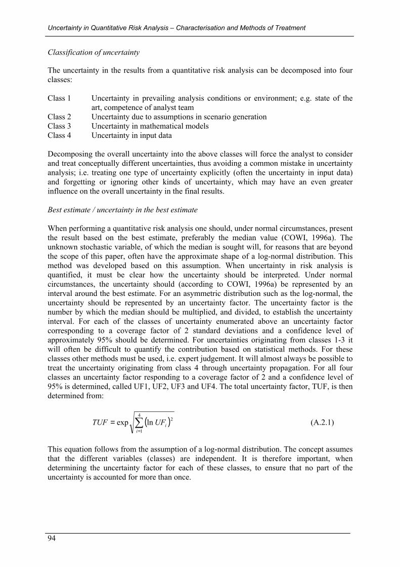
Uncertainty in Quantitative Risk Analysis – Characterisation and Methods of Treatment
94
Classification of uncertainty The uncertainty in the results from a quantitative risk analysis can be decomposed into four classes: Class 1 Uncertainty in prevailing analysis conditions or environment; e.g. state of the
art, competence of analyst team Class 2 Uncertainty due to assumptions in scenario generation Class 3 Uncertainty in mathematical models Class 4 Uncertainty in input data Decomposing the overall uncertainty into the above classes will force the analyst to consider and treat conceptually different uncertainties, thus avoiding a common mistake in uncertainty analysis; i.e. treating one type of uncertainty explicitly (often the uncertainty in input data) and forgetting or ignoring other kinds of uncertainty, which may have an even greater influence on the overall uncertainty in the final results. Best estimate / uncertainty in the best estimate When performing a quantitative risk analysis one should, under normal circumstances, present the result based on the best estimate, preferably the median value (COWI, 1996a). The unknown stochastic variable, of which the median is sought will, for reasons that are beyond the scope of this paper, often have the approximate shape of a log-normal distribution. This method was developed based on this assumption. When uncertainty in risk analysis is quantified, it must be clear how the uncertainty should be interpreted. Under normal circumstances, the uncertainty should (according to COWI, 1996a) be represented by an interval around the best estimate. For an asymmetric distribution such as the log-normal, the uncertainty should be represented by an uncertainty factor. The uncertainty factor is the number by which the median should be multiplied, and divided, to establish the uncertainty interval. For each of the classes of uncertainty enumerated above an uncertainty factor corresponding to a coverage factor of 2 standard deviations and a confidence level of approximately 95% should be determined. For uncertainties originating from classes 1-3 it will often be difficult to quantify the contribution based on statistical methods. For these classes other methods must be used, i.e. expert judgement. It will almost always be possible to treat the uncertainty originating from class 4 through uncertainty propagation. For all four classes an uncertainty factor responding to a coverage factor of 2 and a confidence level of 95% is determined, called UF1, UF2, UF3 and UF4. The total uncertainty factor, TUF, is then determined from:
( )∑=
=4
1
2lnexpi
iUFTUF (A.2.1)
This equation follows from the assumption of a log-normal distribution. The concept assumes that the different variables (classes) are independent. It is therefore important, when determining the uncertainty factor for each of these classes, to ensure that no part of the uncertainty is accounted for more than once.

Appendix 2
95
Determination of uncertainty factors in the different classes There are two alternative methods available to determine the uncertainty factors in each of the different classes. The first, simple method is based on an overall estimate of the uncertainty factor of the whole class. In the second, more sophisticated method, each class of uncertainty is divided into sub-classes, for each of which the uncertainty factor is determined. The uncertainty factor for the whole class is generated in the same manner as the overall uncertainty factor:
( )2/1
1
2lnexp
= ∑=
n
iiUFUF (A.2.2)
Class 1 Uncertainty in prevailing conditions or environment: The uncertainty in the prevailing analysis conditions or environment may originate from the fact that everything is not known about the final construction of the system in the beginning phase of the project. Another reason could be disagreement between experts regarding how to model the system, or lack of knowledge about the fundamental physical or chemical reactions in the system. In Table A.2.1 suggestions are given on ways to determine the uncertainty factor in this class. The table is not exhaustive, and the analyst should, if necessary, make efforts to complete it in order to cover the situation under consideration as fully as possible. Table A.2.1 Suggestions of ways to determine the uncertainty factor in class 1 Small uncertainty
1<UF1<2 Moderate Uncertainty 2<UF1<10
Large uncertainty 10<UF1
Analyst’s experience and competence
Extensive. The analyst is qualified to determine the uncertainties.
Reasonable. The analyst is able to give qualified estimates of most of the uncertainties involved.
Little. The analyst can only give coarse estimates of the uncertainties involved.
Knowledge of background and conditions of the project
Extensive Reasonable Little
Available time and resources
Sufficient Reasonable Lacking
General knowledge base in the specific area
The specific area is well known. There is consensus between experts.
There is some lack of clarity and disagreement between experts.
There is substantial lack of clarity and disagreement between experts.
The uncertainty factor for the other classes of uncertainty is obtained in a similar way, based on tables provided in the guidelines with the same structure as Table A.2.1, but specific for each class. One difference lies in the treatment of the uncertainty in class 4, due to input data. When the uncertainty in each of the input variables is determined, uncertainty propagation is conducted to determine the uncertainty factor of class 4. The uncertainty propagation is conducted using a simulation based on Latin hypercube sampling, possibly combined with the response surface method. The results of uncertainty propagation will nearly always be a graphical representation of the distribution function for the output. These distributions can, in most cases, be approximated by the log-normal distribution, making it possible to find the uncertainty factor UF4 by interpreting the graph. After having determined all the uncertainty factors of the different classes the total uncertainty factor can be obtained by using Eq. (A.2.1).

Uncertainty in Quantitative Risk Analysis – Characterisation and Methods of Treatment
96
Conclusions We conclude that the methodology adopted in the Danish guidelines may provide a rational platform for incorporating all kinds of uncertainty into the analysis. However, to be able to make consistent decisions using an analysis based on this methodology, it would have to be standardised in some way. In its present form quantification of the different uncertainty factors will be subject to biases. For instance, what is to be considered as “Extensive” knowledge of background and conditions of the project, justifying the rating “Small uncertainty” and the corresponding uncertainty factor (1-2) in Table A.2.1? National consensus regarding the prerequisites for the different uncertainty factors must be reached if this approach is to be adopted, to ensure the possibility of comparing analyses carried out by different assessors.
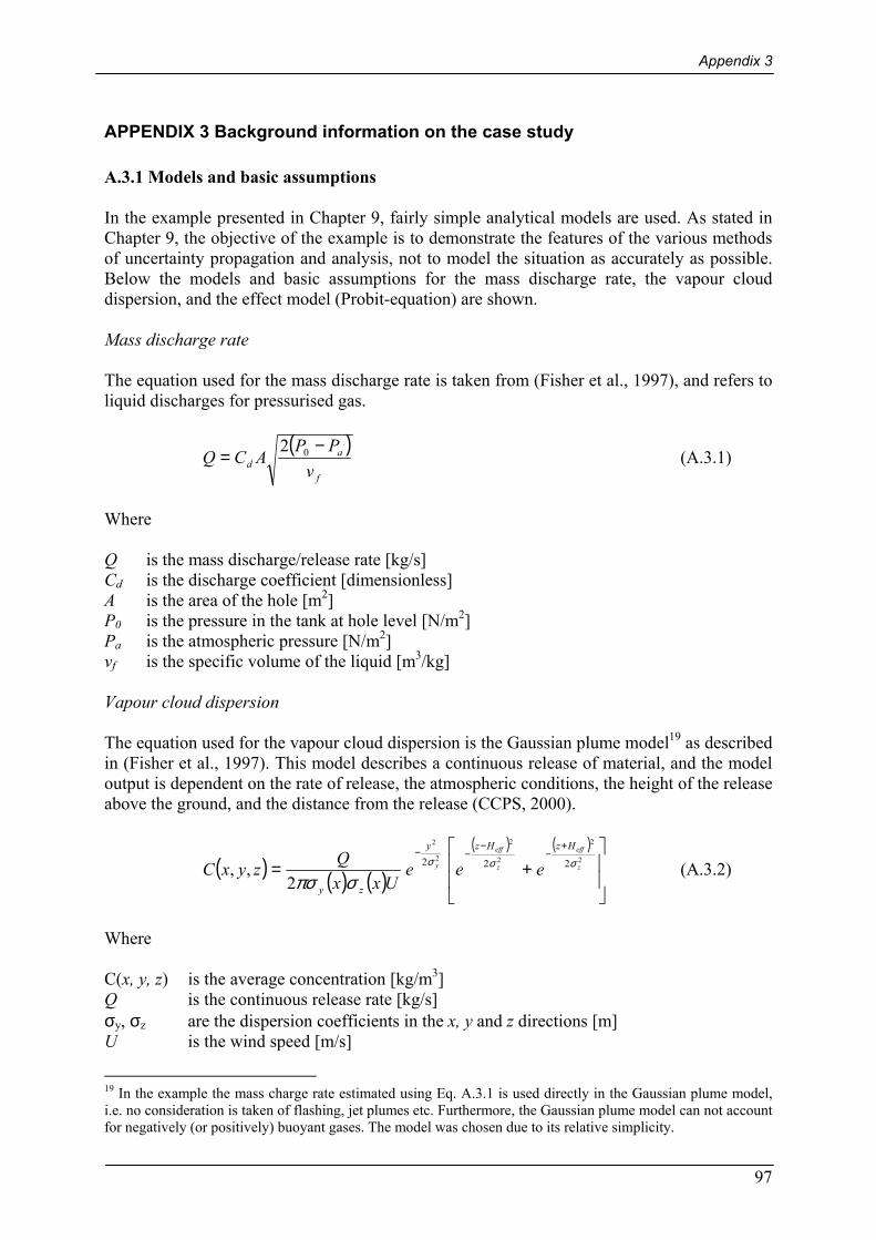
Appendix 3
97
APPENDIX 3 Background information on the case study A.3.1 Models and basic assumptions In the example presented in Chapter 9, fairly simple analytical models are used. As stated in Chapter 9, the objective of the example is to demonstrate the features of the various methods of uncertainty propagation and analysis, not to model the situation as accurately as possible. Below the models and basic assumptions for the mass discharge rate, the vapour cloud dispersion, and the effect model (Probit-equation) are shown. Mass discharge rate The equation used for the mass discharge rate is taken from (Fisher et al., 1997), and refers to liquid discharges for pressurised gas.
( )f
ad v
PPACQ
−= 02
(A.3.1)
Where Q is the mass discharge/release rate [kg/s] Cd is the discharge coefficient [dimensionless] A is the area of the hole [m2] P0 is the pressure in the tank at hole level [N/m2] Pa is the atmospheric pressure [N/m2] vf is the specific volume of the liquid [m3/kg] Vapour cloud dispersion The equation used for the vapour cloud dispersion is the Gaussian plume model19 as described in (Fisher et al., 1997). This model describes a continuous release of material, and the model output is dependent on the rate of release, the atmospheric conditions, the height of the release above the ground, and the distance from the release (CCPS, 2000).
( ) ( ) ( )
( ) ( )
+=
+−
−−−
2
2
2
2
2
2
222
2,, z
eff
z
eff
y
HzHzy
zy
eeeUxx
QzyxC σσσ
σπσ (A.3.2)
Where C(x, y, z) is the average concentration [kg/m3] Q is the continuous release rate [kg/s] σy, σz are the dispersion coefficients in the x, y and z directions [m] U is the wind speed [m/s]
19 In the example the mass charge rate estimated using Eq. A.3.1 is used directly in the Gaussian plume model, i.e. no consideration is taken of flashing, jet plumes etc. Furthermore, the Gaussian plume model can not account for negatively (or positively) buoyant gases. The model was chosen due to its relative simplicity.
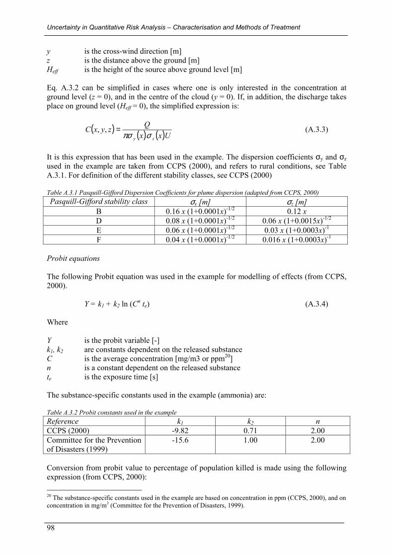
Uncertainty in Quantitative Risk Analysis – Characterisation and Methods of Treatment
98
y is the cross-wind direction [m] z is the distance above the ground [m] Heff is the height of the source above ground level [m] Eq. A.3.2 can be simplified in cases where one is only interested in the concentration at ground level (z = 0), and in the centre of the cloud (y = 0). If, in addition, the discharge takes place on ground level (Heff = 0), the simplified expression is:
( ) ( ) ( )UxxQzyxC
zy σπσ=,, (A.3.3)
It is this expression that has been used in the example. The dispersion coefficients σy and σz used in the example are taken from CCPS (2000), and refers to rural conditions, see Table A.3.1. For definition of the different stability classes, see CCPS (2000) Table A.3.1 Pasquill-Gifford Dispersion Coefficients for plume dispersion (adapted from CCPS, 2000) Pasquill-Gifford stability class σy [m] σz [m]
B 0.16 x (1+0.0001x)-1/2 0.12 x D 0.08 x (1+0.0001x)-1/2 0.06 x (1+0.0015x)-1/2
E 0.06 x (1+0.0001x)-1/2 0.03 x (1+0.0003x)-1
F 0.04 x (1+0.0001x)-1/2 0.016 x (1+0.0003x)-1 Probit equations The following Probit equation was used in the example for modelling of effects (from CCPS, 2000). Y = k1 + k2 ln (Cn te) (A.3.4) Where Y is the probit variable [-] k1, k2 are constants dependent on the released substance C is the average concentration [mg/m3 or ppm20] n is a constant dependent on the released substance te is the exposure time [s] The substance-specific constants used in the example (ammonia) are: Table A.3.2 Probit constants used in the example Reference k1 k2 n CCPS (2000) -9.82 0.71 2.00 Committee for the Prevention of Disasters (1999)
-15.6 1.00 2.00
Conversion from probit value to percentage of population killed is made using the following expression (from CCPS, 2000): 20 The substance-specific constants used in the example are based on concentration in ppm (CCPS, 2000), and on concentration in mg/m3 (Committee for the Prevention of Disasters, 1999).
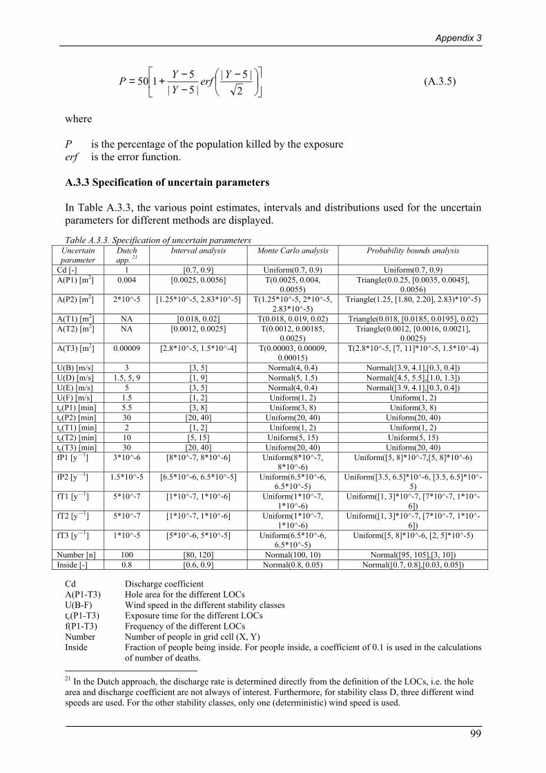
Appendix 3
99
−−−+=
2|5|
|5|5150 Yerf
YYP (A.3.5)
where P is the percentage of the population killed by the exposure erf is the error function. A.3.3 Specification of uncertain parameters In Table A.3.3, the various point estimates, intervals and distributions used for the uncertain parameters for different methods are displayed. Table A.3.3. Specification of uncertain parameters
Uncertain parameter
Dutch app. 21
Interval analysis Monte Carlo analysis Probability bounds analysis
Cd [-] 1 [0.7, 0.9] Uniform(0.7, 0.9) Uniform(0.7, 0.9) A(P1) [m2] 0.004 [0.0025, 0.0056] T(0.0025, 0.004,
0.0055) Triangle(0.0.25, [0.0035, 0.0045],
0.0056) A(P2) [m2] 2*10^-5 [1.25*10^-5, 2.83*10^-5] T(1.25*10^-5, 2*10^-5,
2.83*10^-5) Triangle(1.25, [1.80, 2.20], 2.83)*10^-5)
A(T1) [m2] NA [0.018, 0.02] T(0.018, 0.019, 0.02) Triangle(0.018, [0.0185, 0.0195], 0.02) A(T2) [m2] NA [0.0012, 0.0025] T(0.0012, 0.00185,
0.0025) Triangle(0.0012, [0.0016, 0.0021],
0.0025) A(T3) [m2] 0.00009 [2.8*10^-5, 1.5*10^-4] T(0.00003, 0.00009,
0.00015) T(2.8*10^-5, [7, 11]*10^-5, 1.5*10^-4)
U(B) [m/s] 3 [3, 5] Normal(4, 0.4) Normal([3.9, 4.1],[0.3, 0.4]) U(D) [m/s] 1.5, 5, 9 [1, 9] Normal(5, 1.5) Normal([4.5, 5.5],[1.0, 1.3]) U(E) [m/s] 5 [3, 5] Normal(4, 0.4) Normal([3.9, 4.1],[0.3, 0.4]) U(F) [m/s] 1.5 [1, 2] Uniform(1, 2) Uniform(1, 2) tc(P1) [min] 5.5 [3, 8] Uniform(3, 8) Uniform(3, 8) tc(P2) [min] 30 [20, 40] Uniform(20, 40) Uniform(20, 40) tc(T1) [min] 2 [1, 2] Uniform(1, 2) Uniform(1, 2) tc(T2) [min] 10 [5, 15] Uniform(5, 15) Uniform(5, 15) tc(T3) [min] 30 [20, 40] Uniform(20, 40) Uniform(20, 40) fP1 [y—1] 3*10^-6 [8*10^-7, 8*10^-6] Uniform(8*10^-7,
8*10^-6) Uniform([5, 8]*10^-7,[5, 8]*10^-6)
fP2 [y—1] 1.5*10^-5 [6.5*10^-6, 6.5*10^-5] Uniform(6.5*10^-6, 6.5*10^-5)
Uniform([3.5, 6.5]*10^-6, [3.5, 6.5]*10^-5)
fT1 [y—1] 5*10^-7 [1*10^-7, 1*10^-6] Uniform(1*10^-7, 1*10^-6)
Uniform([1, 3]*10^-7, [7*10^-7, 1*10^-6])
fT2 [y—1] 5*10^-7 [1*10^-7, 1*10^-6] Uniform(1*10^-7, 1*10^-6)
Uniform([1, 3]*10^-7, [7*10^-7, 1*10^-6])
fT3 [y—1] 1*10^-5 [5*10^-6, 5*10^-5] Uniform(6.5*10^-6, 6.5*10^-5)
Uniform([5, 8]*10^-6, [2, 5]*10^-5)
Number [n] 100 [80, 120] Normal(100, 10) Normal([95, 105],[3, 10]) Inside [-] 0.8 [0.6, 0.9] Normal(0.8, 0.05) Normal([0.7, 0.8],[0.03, 0.05])
Cd Discharge coefficient A(P1-T3) Hole area for the different LOCs U(B-F) Wind speed in the different stability classes tc(P1-T3) Exposure time for the different LOCs f(P1-T3) Frequency of the different LOCs Number Number of people in grid cell (X, Y) Inside Fraction of people being inside. For people inside, a coefficient of 0.1 is used in the calculations
of number of deaths. 21 In the Dutch approach, the discharge rate is determined directly from the definition of the LOCs, i.e. the hole area and discharge coefficient are not always of interest. Furthermore, for stability class D, three different wind speeds are used. For the other stability classes, only one (deterministic) wind speed is used.
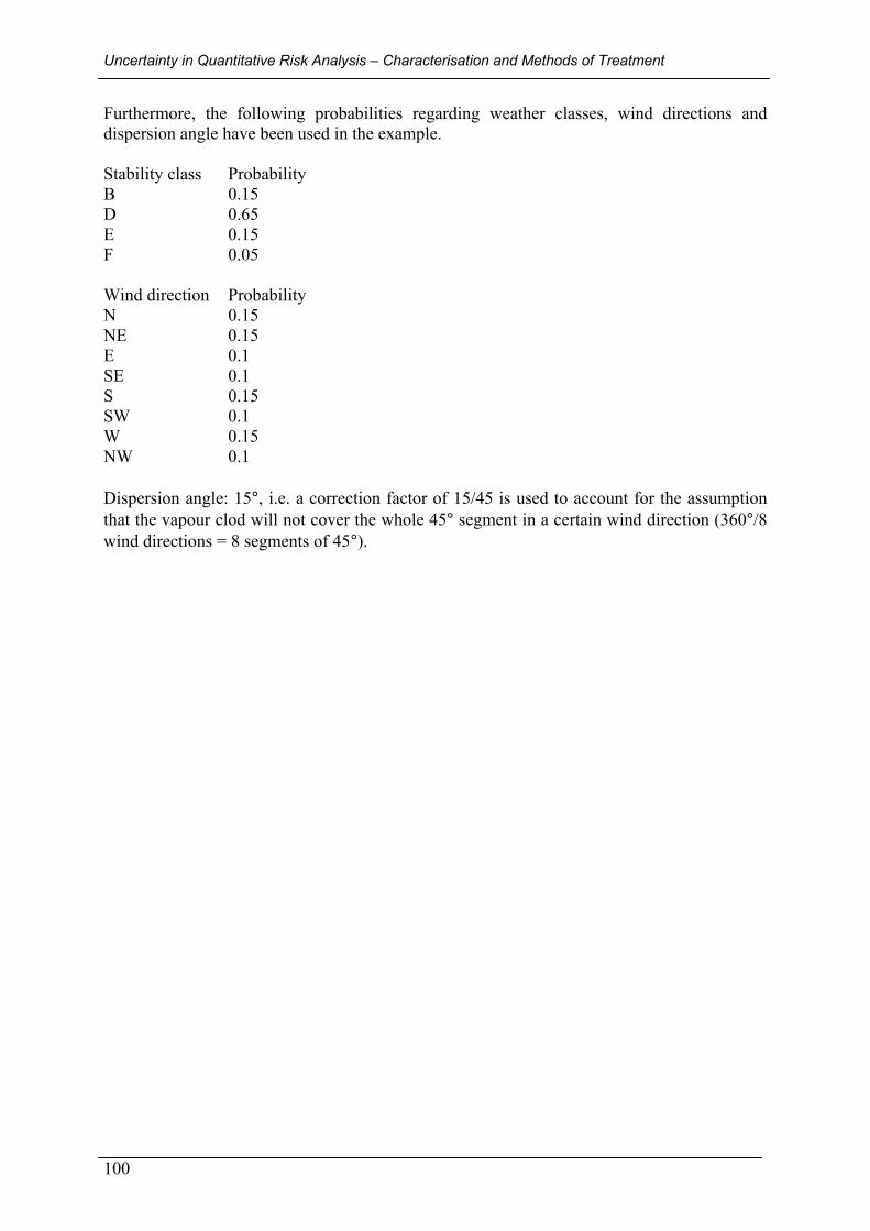
Uncertainty in Quantitative Risk Analysis – Characterisation and Methods of Treatment
100
Furthermore, the following probabilities regarding weather classes, wind directions and dispersion angle have been used in the example. Stability class Probability B 0.15 D 0.65 E 0.15 F 0.05 Wind direction Probability N 0.15 NE 0.15 E 0.1 SE 0.1 S 0.15 SW 0.1 W 0.15 NW 0.1 Dispersion angle: 15°, i.e. a correction factor of 15/45 is used to account for the assumption that the vapour clod will not cover the whole 45° segment in a certain wind direction (360°/8 wind directions = 8 segments of 45°).
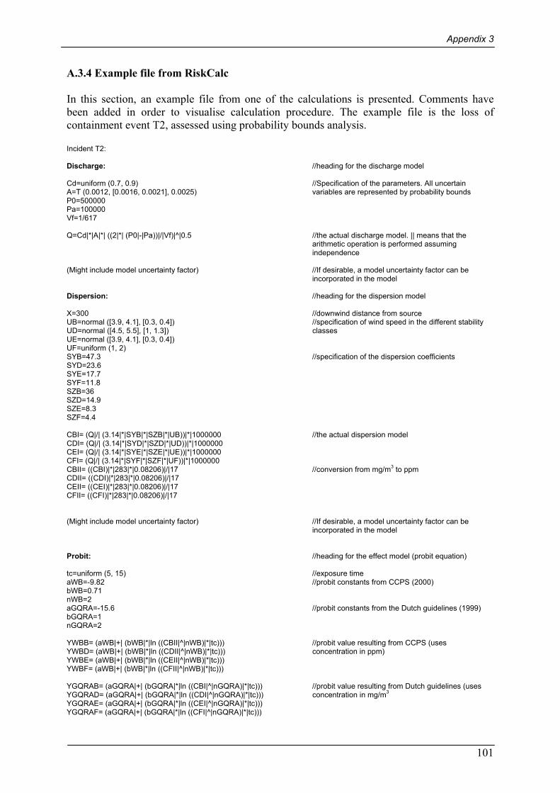
Appendix 3
101
A.3.4 Example file from RiskCalc In this section, an example file from one of the calculations is presented. Comments have been added in order to visualise calculation procedure. The example file is the loss of containment event T2, assessed using probability bounds analysis. Incident T2: Discharge: //heading for the discharge model Cd=uniform (0.7, 0.9) //Specification of the parameters. All uncertain A=T (0.0012, [0.0016, 0.0021], 0.0025) variables are represented by probability bounds P0=500000 Pa=100000 Vf=1/617 Q=Cd|*|A|*| ((2|*| (P0|-|Pa))|/|Vf)|^|0.5 //the actual discharge model. || means that the arithmetic operation is performed assuming independence (Might include model uncertainty factor) //If desirable, a model uncertainty factor can be incorporated in the model Dispersion: //heading for the dispersion model X=300 //downwind distance from source UB=normal ([3.9, 4.1], [0.3, 0.4]) //specification of wind speed in the different stability UD=normal ([4.5, 5.5], [1, 1.3]) classes UE=normal ([3.9, 4.1], [0.3, 0.4]) UF=uniform (1, 2) SYB=47.3 //specification of the dispersion coefficients SYD=23.6 SYE=17.7 SYF=11.8 SZB=36 SZD=14.9 SZE=8.3 SZF=4.4 CBI= (Q|/| (3.14|*|SYB|*|SZB|*|UB))|*|1000000 //the actual dispersion model CDI= (Q|/| (3.14|*|SYD|*|SZD|*|UD))|*|1000000 CEI= (Q|/| (3.14|*|SYE|*|SZE|*|UE))|*|1000000 CFI= (Q|/| (3.14|*|SYF|*|SZF|*|UF))|*|1000000 CBII= ((CBI)|*|283|*|0.08206)|/|17 //conversion from mg/m3 to ppm CDII= ((CDI)|*|283|*|0.08206)|/|17 CEII= ((CEI)|*|283|*|0.08206)|/|17 CFII= ((CFI)|*|283|*|0.08206)|/|17 (Might include model uncertainty factor) //If desirable, a model uncertainty factor can be incorporated in the model Probit: //heading for the effect model (probit equation) tc=uniform (5, 15) //exposure time aWB=-9.82 //probit constants from CCPS (2000) bWB=0.71 nWB=2 aGQRA=-15.6 //probit constants from the Dutch guidelines (1999) bGQRA=1 nGQRA=2 YWBB= (aWB|+| (bWB|*|ln ((CBII|^|nWB)|*|tc))) //probit value resulting from CCPS (uses YWBD= (aWB|+| (bWB|*|ln ((CDII|^|nWB)|*|tc))) concentration in ppm) YWBE= (aWB|+| (bWB|*|ln ((CEII|^|nWB)|*|tc))) YWBF= (aWB|+| (bWB|*|ln ((CFII|^|nWB)|*|tc))) YGQRAB= (aGQRA|+| (bGQRA|*|ln ((CBI|^|nGQRA)|*|tc))) //probit value resulting from Dutch guidelines (uses YGQRAD= (aGQRA|+| (bGQRA|*|ln ((CDI|^|nGQRA)|*|tc))) concentration in mg/m3 YGQRAE= (aGQRA|+| (bGQRA|*|ln ((CEI|^|nGQRA)|*|tc))) YGQRAF= (aGQRA|+| (bGQRA|*|ln ((CFI|^|nGQRA)|*|tc)))

Uncertainty in Quantitative Risk Analysis – Characterisation and Methods of Treatment
102
export YWBB, YWBD, YWBE, YWBF, YGQRAB, YGQRAD, YGQRAE, YGQRAF Exporting variable to YGQRAF.prn Exporting variable to YGQRAE.prn //the distributions of the probit values are exported Exporting variable to YGQRAD.prn and converted to distributions of probability of death Exporting variable to YGQRAB.prn using Microsoft Excel Exporting variable to YWBF.prn Exporting variable to YWBE.prn Exporting variable to YWBD.prn Exporting variable to YWBB.prn (Conversion from probit to probability of death is made using Microsoft Excel.) import YWBB //the converted variables are imported Importing variable from YWBB.prn import YWBD Importing variable from YWBD.prn import YWBE Importing variable from YWBE.prn import YWBF Importing variable from YWBF.prn import YGQRAB Importing variable from YGQRAB.prn import YGQRAD Importing variable from YGQRAD.prn import YGQRAE Importing variable from YGQRAE.prn import YGQRAF Importing variable from YGQRAF.prn PWBB=YWBB //change of name to indicate that they now refer to PWBD=YWBD distributions of the probability of death PWBE=YWBE PWBF=YWBF PGQRAB=YGQRAB PGQRAD=YGQRAD PGQRAE=YGQRAE PGQRAF=YGQRAF PDB=env (PWBB, PGQRAB) //the union of the two uncertain numbers (i.e. the PDD=env (PWBD, PGQRAD) probability bounds for the probability of death PDE=env (PWBE, PGQRAE) generated using CCPS and the Dutch guidelines) PDF=env (PWBF, PGQRAF) are constructed and used further in the analysis Frequencies & probabilities: //heading fTII=uniform ([1*10^-7, 3*10^-7], [7*10^-7, 1*10^-6]) //specification of the (uncertain) frequency for LOC T2 PB=0.15 //probabilities for the different stability classes PD=0.65 PE=0.15 PF=0.05 PE=0.1 //probability that the vapour clod will travel to the east , i.e. towards grid point (X, Y) Ang=1/3 //reduction factor for the “dispersion angle”, see Section 9 Individual risk calculation: //heading IRTIIB=fTII|*|PB|*|PNE|*|Ang|*|PDB/100 //calculation of the contributions to the total individual risk from the different stability classes IRTIID=fTII|*|PD|*|PNE|*|Ang|*|PDD/100 IRTIIE=fTII|*|PE|*|PNE|*|Ang|*|PDE/100 IRTIIF=fTII|*|PF|*|PNE|*|Ang|*|PDF/100 IRTII=IRTIIB|+|IRTIID|+|IRTIIE|+|IRTIIF //calculation of the total individual risk from LOC T2
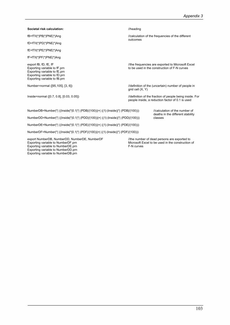
Appendix 3
103
Societal risk calculation: //heading fB=fTII|*|PB|*|PNE|*|Ang //calculation of the frequencies of the different outcomes fD=fTII|*|PD|*|PNE|*|Ang fE=fTII|*|PE|*|PNE|*|Ang fF=fTII|*|PF|*|PNE|*|Ang export fB, fD, fE, fF //the frequencies are exported to Microsoft Excel Exporting variable to fF.prn to be used in the construction of F-N curves Exporting variable to fE.prn Exporting variable to fD.prn Exporting variable to fB.prn Number=normal ([95,105], [3, 6]) //definition of the (uncertain) number of people in grid cell (X, Y) Inside=normal ([0.7, 0.8], [0.03, 0.05]) //definition of the fraction of people being inside. For people inside, a reduction factor of 0.1 is used NumberDB=Number|*| ((Inside|*|0.1|*| (PDB|/|100))|+| ((1|-|Inside)|*| (PDB|/|100))) //calculation of the number of deaths in the different stability NumberDD=Number|*| ((Inside|*|0.1|*| (PDD|/|100))|+| ((1|-|Inside)|*| (PDD|/|100))) classes NumberDE=Number|*| ((Inside|*|0.1|*| (PDE|/|100))|+| ((1|-|Inside)|*| (PDE|/|100))) NumberDF=Number|*| ((Inside|*|0.1|*| (PDF|/|100))|+| ((1|-|Inside)|*| (PDF|/|100))) export NumberDB, NumberDD, NumberDE, NumberDF //the number of dead persons are exported to Exporting variable to NumberDF.prn Microsoft Excel to be used in the construction of Exporting variable to NumberDE.prn F-N curves Exporting variable to NumberDD.prn Exporting variable to NumberDB.prn