uncertainty as a barrier to adoption of mitigation
TRANSCRIPT

HAL Id: tel-02484561https://hal.univ-lorraine.fr/tel-02484561
Submitted on 19 Feb 2020
HAL is a multi-disciplinary open accessarchive for the deposit and dissemination of sci-entific research documents, whether they are pub-lished or not. The documents may come fromteaching and research institutions in France orabroad, or from public or private research centers.
L’archive ouverte pluridisciplinaire HAL, estdestinée au dépôt et à la diffusion de documentsscientifiques de niveau recherche, publiés ou non,émanant des établissements d’enseignement et derecherche français ou étrangers, des laboratoirespublics ou privés.
Uncertainty as a barrier to adoption of mitigationpractices in the agricultural sector
Camille Tevenart
To cite this version:Camille Tevenart. Uncertainty as a barrier to adoption of mitigation practices in the agriculturalsector. Economics and Finance. Université de Lorraine, 2019. English. �NNT : 2019LORR0156�.�tel-02484561�

AVERTISSEMENT
Ce document est le fruit d'un long travail approuvé par le jury de soutenance et mis à disposition de l'ensemble de la communauté universitaire élargie. Il est soumis à la propriété intellectuelle de l'auteur. Ceci implique une obligation de citation et de référencement lors de l’utilisation de ce document. D'autre part, toute contrefaçon, plagiat, reproduction illicite encourt une poursuite pénale. Contact : [email protected]
LIENS Code de la Propriété Intellectuelle. articles L 122. 4 Code de la Propriété Intellectuelle. articles L 335.2- L 335.10 http://www.cfcopies.com/V2/leg/leg_droi.php http://www.culture.gouv.fr/culture/infos-pratiques/droits/protection.htm

THESE
École doctorale no 79Sciences Juridiques, Politiques, Économiques et de Gestion
Doctorat
THÈSE
pour obtenir le grade de docteur délivré par
l’Université de LorraineSpécialité doctorale “Sciences Économiques”
présentée et soutenue publiquement par
Camille TEVENART
le 16 octobre 2019
L’incertitude en tant que frein à l’adoption de mesuresd’atténuation en agriculture
Directrices de thèse :Marielle BRUNETTE
Caroline ORSET
JuryMme Géraldine BOCQUEHO, Chargé de recherche INRA, BETA ExaminatriceM Olivier DESCHENES, Professeur, University of California ExaminateurM Pierre DUPRAZ, Directeur de recherche INRA, SMART-LERECO ExaminateurMme Marie-Hélène HUBERT, Maître de conférences, Université de Rennes RapporteurM Arnaud REYNAUD, Directeur de recherche INRA, TSE Rapporteur
Bureau d’Économie Théorique et Appliquée (BETA),UMR Université de Lorraine, Université de Strasbourg, AgroParisTech, CNRS, INRA.

A ma fille AndréaEt mon épouse Nemdia
ii

Acknowledgements
After more than three years of research, I finally have the opportunity to present themajor part of my work in this thesis. All this production would not have been possiblewithout the support of many people, who assisted me from the beginning.
I would like to thank, first of all, my supervisors Marielle Brunette, Researcher at theBETA Nancy laboratory of Lorraine University, and Caroline Orset, Professor at the PublicEconomics laboratory of INRA-AgroParisTech, for their constant support all along theseyears. Their precious advices were of great help, especially during hard times. I also wantto thank Philippe Delacote, who never failed at finding practical solutions when needed.Many thanks also to Marc Baudry for his strong intellectual support and his occasionalassistance when I was facing complex research problems. I would like to give particularacknowledgements to Christian de Perthuis, for his support and his ability to trust and toappreciate the work of his students. Many thanks to Antoine Poupart, from AgroSolutions(InVivo group) for his trust and his feedbacks about my work.
I would like to give thanks to Marie-Hélène Hubert, Assitant Professor at the Eco-nomics Department of Rennes University, and Arnaud Reynaud, Head of the TSE-R lab-oratory of Toulouse School of Economics, for having accepted to be the referees of mythesis. This is an honor for me to see my work being reviewed by them.
Further thanks go to Géraldine Bocquého, Researcher at the BETA Nancy laboratory ofLorraine University, and Pierre Dupraz, Head of the SMART-LERECO laboratory of INRARennes, for being examiners of my thesis. Special thanks go to Olivier Deschênes, Profes-sor at the Economics Department of the University of California, Santa Barbara for havingagreed to come from such a long distance and to be a part of my thesis jury. I am veryproud to say that my thesis has been discussed by these researchers.
I want to thank a lot Professor Andrew Plantinga, from the Bren School of Environ-mental Sciences and Management of the University of California, Santa Barbara, for hav-ing hosted me during four months at the Bren School. Not only his scientific advices, butalso his kindness, sympathy and hospitality were of a great importance for me in theselast years.
Several researchers I met during these years participated, through their advices, feed-backs, cooperation or assistance, to this research. To quote some of them, Nathalie De-lame, Hervé Dakpo, Raja Chakir, Serge Garcia, Danae Hernandez-Cortes, ChristopherCostello, Kyle Meng, Olivier Damette, among others, deserve thanks for their support atdifferent levels.
I would like to thank the farmers and the cooperatives’ agents that agreed to havemeetings with me for the field experiment, and the support of AgroSolutions’ engineersfor their help in the making of the survey.
I would like to give a huge thank to my partners PhD candidates and young researchers,with who I shared many good times (and some less happy times), among them, DavidSoares, Julien Wolfersberger, Olivier Rebenaque, Salomé Bakaloglou, Liza Dorinet, friendsfrom the Climate Economics Chaire, the Public Economics laboratory and the BETA Nancy,people I met in France or during my visiting in the States. I won’t forget your presence bymy side and your active or passive support.
iii

Last but not least, I would like to thank my wife, family and friends. And I want toexpress my gratitude for all that has been given and received.
iv

Contents
Contents v
List of Figures vii
List of Tables ix
1 Introductory chapter 11.1 Mitigation of environmental externalities related to agricultural practices’
emissions . . . . . . . . . . . . . . . . . . . . . . . . . . . . . . . . . . . . . . . . 31.2 Limitations to the adoption of new farming practices: the market failures
associated to uncertainties . . . . . . . . . . . . . . . . . . . . . . . . . . . . . 71.3 Contributions . . . . . . . . . . . . . . . . . . . . . . . . . . . . . . . . . . . . . 14
2 Adoption of mitigation practices in agriculture: an application of the real optiontheory 232.1 Introduction . . . . . . . . . . . . . . . . . . . . . . . . . . . . . . . . . . . . . . 242.2 Exogenous learning process . . . . . . . . . . . . . . . . . . . . . . . . . . . . . 272.3 The risk neutral farmer . . . . . . . . . . . . . . . . . . . . . . . . . . . . . . . . 282.4 The risk averse farmer . . . . . . . . . . . . . . . . . . . . . . . . . . . . . . . . 302.5 Endogenous learning process . . . . . . . . . . . . . . . . . . . . . . . . . . . . 332.6 Discussion . . . . . . . . . . . . . . . . . . . . . . . . . . . . . . . . . . . . . . . 36
Appendices 45
3 Yields volatility and friction in land conversion 513.1 Introduction . . . . . . . . . . . . . . . . . . . . . . . . . . . . . . . . . . . . . . 523.2 Literature review . . . . . . . . . . . . . . . . . . . . . . . . . . . . . . . . . . . 533.3 Land allocation and uncertainty measures . . . . . . . . . . . . . . . . . . . . 573.4 Empirical application . . . . . . . . . . . . . . . . . . . . . . . . . . . . . . . . 623.5 Results assuming exogeneity of explanatory variables . . . . . . . . . . . . . 663.6 Instrumental regression . . . . . . . . . . . . . . . . . . . . . . . . . . . . . . . 693.7 Conclusion . . . . . . . . . . . . . . . . . . . . . . . . . . . . . . . . . . . . . . . 72
Appendices 79
4 Role of farmers’ risk and ambiguity preferences on fertilization decisions: an ex-periment 994.1 Introduction . . . . . . . . . . . . . . . . . . . . . . . . . . . . . . . . . . . . . . 1004.2 Literature review . . . . . . . . . . . . . . . . . . . . . . . . . . . . . . . . . . . 1014.3 Questionnaire . . . . . . . . . . . . . . . . . . . . . . . . . . . . . . . . . . . . . 1034.4 Results . . . . . . . . . . . . . . . . . . . . . . . . . . . . . . . . . . . . . . . . . 106
v
CONTENTS
4.5 Conclusion . . . . . . . . . . . . . . . . . . . . . . . . . . . . . . . . . . . . . . . 118
Appendices 125
5 Concluding comments 1335.1 Uncertainty, irreversibility and information at the core of farmers’ reluc-
tance to adopt . . . . . . . . . . . . . . . . . . . . . . . . . . . . . . . . . . . . . 1345.2 Volatility in grass yields can prevent us from taking benefits from the poten-
tial of grasslands carbon sink . . . . . . . . . . . . . . . . . . . . . . . . . . . . 1355.3 Not only risk but ambiguity aversion impact N2O emissions mitigation re-
lated to nitrogenous fertilization practices . . . . . . . . . . . . . . . . . . . . 136
6 Summary of the thesis (French) 139
vi

List of Figures
1.1 MACC from Bamière et al. [5] -INRA . . . . . . . . . . . . . . . . . . . . . . . . 51.2 Inefficiency of flat subsidies with hidden costs - author . . . . . . . . . . . . 15
1 Partial adjustement of adoption w.r.t. potential bad scenario - author. fore-casts . . . . . . . . . . . . . . . . . . . . . . . . . . . . . . . . . . . . . . . . . . . 49
4.1 Number of safe choices selected by the farmers . . . . . . . . . . . . . . . . . 1064.2 Number of risky choices selected by the farmers . . . . . . . . . . . . . . . . . 1064.3 Number of risky choices selected by the farmers . . . . . . . . . . . . . . . . . 1074.4 Relationship between actual and objective yields . . . . . . . . . . . . . . . . 1104.5 Deviation rate between actual and objective yields . . . . . . . . . . . . . . . 1104.6 Relationship between actual and adviced fertilization . . . . . . . . . . . . . 1114.7 Relationship between actual and adviced first application . . . . . . . . . . . 113
vii

LIST OF FIGURES
viii

List of Tables
3.1 Descriptive statistics . . . . . . . . . . . . . . . . . . . . . . . . . . . . . . . . . 632 URT1 . . . . . . . . . . . . . . . . . . . . . . . . . . . . . . . . . . . . . . . . . . 813 URT2 . . . . . . . . . . . . . . . . . . . . . . . . . . . . . . . . . . . . . . . . . . 814 URT3 . . . . . . . . . . . . . . . . . . . . . . . . . . . . . . . . . . . . . . . . . . 825 URT4 . . . . . . . . . . . . . . . . . . . . . . . . . . . . . . . . . . . . . . . . . . 826 URT5 . . . . . . . . . . . . . . . . . . . . . . . . . . . . . . . . . . . . . . . . . . 837 URT6 . . . . . . . . . . . . . . . . . . . . . . . . . . . . . . . . . . . . . . . . . . 838 URT7 . . . . . . . . . . . . . . . . . . . . . . . . . . . . . . . . . . . . . . . . . . 849 URT8 . . . . . . . . . . . . . . . . . . . . . . . . . . . . . . . . . . . . . . . . . . 8410 URT9 . . . . . . . . . . . . . . . . . . . . . . . . . . . . . . . . . . . . . . . . . . 8511 URT10 . . . . . . . . . . . . . . . . . . . . . . . . . . . . . . . . . . . . . . . . . 8512 URT11 . . . . . . . . . . . . . . . . . . . . . . . . . . . . . . . . . . . . . . . . . 8613 URT12 . . . . . . . . . . . . . . . . . . . . . . . . . . . . . . . . . . . . . . . . . 8614 Control regressions for time effects and multicolinearity . . . . . . . . . . . . 8715 Yields shocks’ impact on Temporary grasslands ratio . . . . . . . . . . . . . . 8816 Yields shocks’ impact on Artificial grasslands ratio . . . . . . . . . . . . . . . 8917 Yields shocks’ impact on Natural and old-seeded grasslands ratio . . . . . . 9018 All yields shocks’ impact on the three types of grasslands . . . . . . . . . . . 9119 Yields volatility (Ornstein-Ulhenbeck)’s impact on Temporary grasslands ratio 9220 Yields volatility (Ornstein-Ulhenbeck)’s impact on Artificial grasslands ratio 9221 Yields volatility (Ornstein-Ulhenbeck)’s impact on Natural and old-seeded
grasslands ratio . . . . . . . . . . . . . . . . . . . . . . . . . . . . . . . . . . . . 9322 Yields volatility (Moving average)’s impact on Temporary grasslands ratio . 9323 Yields volatility (Moving average)’s impact on Artificial grasslands ratio . . . 9424 Yields volatility (Moving average)’s impact on Natural and old-seeded grass-
lands ratio . . . . . . . . . . . . . . . . . . . . . . . . . . . . . . . . . . . . . . . 9425 Yields volatility (Ornstein-Uhlenbeck)’s impact with controls on all grass-
lands ratio . . . . . . . . . . . . . . . . . . . . . . . . . . . . . . . . . . . . . . . 9526 Yields volatility (Moving average)’s impact with controls on all grasslands ratio 9527 Correlation coefficients table for volatility measures (Ornstein-Uhlenbeck)
and meteorological data . . . . . . . . . . . . . . . . . . . . . . . . . . . . . . . 9628 Correlation coefficients table for volatility measures (Moving average) and
meteorological data . . . . . . . . . . . . . . . . . . . . . . . . . . . . . . . . . 9629 Instrumentation of yields volatility (Ornstein Uhlenbeck)’s impact on all grass-
lands ratios . . . . . . . . . . . . . . . . . . . . . . . . . . . . . . . . . . . . . . . 9730 Instrumentation of yields volatility (Moving average)’s impact on all grass-
lands ratios . . . . . . . . . . . . . . . . . . . . . . . . . . . . . . . . . . . . . . . 98
4.1 Risk aversion classification based on lottery choices . . . . . . . . . . . . . . 104
ix

LIST OF TABLES
4.2 Ambiguity aversion classification based on lottery choices . . . . . . . . . . . 1044.3 Cross table function of the modality . . . . . . . . . . . . . . . . . . . . . . . . 1084.4 Pearson correlation coefficients . . . . . . . . . . . . . . . . . . . . . . . . . . 1084.5 Distribution of farmer’s revenues . . . . . . . . . . . . . . . . . . . . . . . . . . 1144.6 Total fertilization . . . . . . . . . . . . . . . . . . . . . . . . . . . . . . . . . . . 1164.7 Fertilization at the first splitting . . . . . . . . . . . . . . . . . . . . . . . . . . 1178 The ten-paired lottery-choice decisions under risk . . . . . . . . . . . . . . . 1279 The ten-paired lottery-choice decisions under ambiguity . . . . . . . . . . . 127
x
Chapter 1
Introductory chapter
Contents1.1 Mitigation of environmental externalities related to agricultural prac-
tices’ emissions . . . . . . . . . . . . . . . . . . . . . . . . . . . . . . . . . . 3
1.1.1 Typology of mitigation practices . . . . . . . . . . . . . . . . . . . . . 3
1.1.2 The cost of mitigating: economic point of view and adoption de-terminants . . . . . . . . . . . . . . . . . . . . . . . . . . . . . . . . . . 5
1.2 Limitations to the adoption of new farming practices: the market fail-ures associated to uncertainties . . . . . . . . . . . . . . . . . . . . . . . . 7
1.2.1 What uncertainties are we talking about? . . . . . . . . . . . . . . . . 7
1.2.2 Risk, risk preferences and risk hedging . . . . . . . . . . . . . . . . . 8
1.2.3 Uncertainty, innovations and informational externalities . . . . . . 10
1.2.4 Beyond risk, ambiguity: an intrinsic limit of the agricultural advise-ment process and use of information . . . . . . . . . . . . . . . . . . 11
1.3 Contributions . . . . . . . . . . . . . . . . . . . . . . . . . . . . . . . . . . . 14
1

CHAPTER 1. INTRODUCTORY CHAPTER
Reducing GHG emissions in the agricultural sector is nowadays considered, in Franceespecially, as a major environmental policy challenge. In 2017, the French agriculturalsector was responsible for 20.4% of the total GHG emissions in France, especially throughnitrous oxide (N2O) and methane (CH4) emissions, and in a marginal way through carbondioxide (CITEPA [16]). It is also the main sector, in parallel with forest, able to sequesteratmospheric carbon and thus represents a great potential of climate change mitigationand a key feature of carbon neutrality. Kyoto (1997) and Göteborg (2012) protocols ledFrance toward the implementation of emissions mitigation. In the same vein, the "Pa-quet Énergie-Climat" of the European Union, revised in 2014, asks to France a reductionof 40% of its emissions compared to 1990. The French energy market being essentiallyrepresented by the nuclear power, that is not a big emissions producers and which, in allcase, is not flexible enough to adopt further important mitigations, it is important to tar-get other sectors, like the agricultural sector, which furthermore has a important size inthe country (De Cara and Jayet [17]). Regarding more specifically the agricultural sector, asuccession of laws, coming from the "Grenelle de l’environnement" in 2009, and from the"Loi d’avenir" of the 2014, October 13th , about mitigation have been voted between 2005and 2015. "Agri-environmental and Climate Schemes" (AECS) have been emphasized in2015 (European Common Agricultural Policy, CAP), providing specifications about thesubsidized measures farmers can adopt to limit their impact on the environment and de-velop their "integration" in their local ecosystem, but in a context of decreasing budget.The measures generally encourage farmers to diversify their activities, integrate legumi-nous crop, improve land rotation, develop better link between a good feeding for the live-stock and vegetal protein production, and especially limit the use of pollutant inputs.
However, mitigation as well as conservation practices, are deemed far from being mas-sively adopted nowadays. Despite the lack of complete statistics about individual effortsmade by farmers, agricultural emissions have been reduced, since 1990, twice lower thanthe total emissions’ reduction rate in France1. New practices can have a low speed of dif-fusion in the agricultural sector. We have good examples of that phenomenon: "organicfarming" represented around 6% of the total French agricultural area2, while conservationprograms like Ecophyto failed to reduce chemical pesticide uses (moreover, an increasein chemicals use has been recorded during the period of the project, due, inter alia, tobad pedoclimatic conditions)3. Moreover new policies have been designed (AECS for in-stance) in order to try new ways to encourage adoption of mitigation practice at the farmlevel, because the farming sector is exempted from the EU-ETS and of any carbon taxon production, and the European Union’s emissions targets and the pressures from theCOP21 have accelerated the implementation of public intervention. While some mitiga-tion practices are associated to a higher level of productive efficiency and related poten-tial benefits, their spread is still limited in France, which encourages the conception ofnew incentives or an improvement of existing ones. There is a need for the identifica-tion and resolution of the causes of non adoption by farmers, and especially, this thesisaims at identifying the role of uncertainty as a hidden cost associated to the adoption ofnew practices. Since uncertainty can impact new practices’ profits evaluation by farm-ers through different drivers, we will identify in which cases it can become a barrier ofadoption. Different methodologies will be used (theoretical, empirical) in order to answer
1Around 9% in 2013 according to the CITEPA [16].2According to the Agence Française pour le Développement et la Promotion de l’Agriculture Biologique.3This State program concerned around 30000 farms, that is equal to around 5% of the amount of farms
in France.
2

CHAPTER 1. INTRODUCTORY CHAPTER
these issues. The existence of hidden costs and benefits of the main mitigation practiceshas to be taken into account to design efficient incentives and policies, and to improve theknowledge about the factors of non adoption. Targeting farmers with appropriate tools inorder to help them adopting mitigation practices can lead to improvements in the alloca-tion of public expenses.
In section 1.1, we briefly describe mitigation practices and the associated economiccosts. In section 1.2, we show how uncertainty can lead to failures for the agriculturalsector to meet the reduction targets. We present the different drivers through which un-certainty can be a barrier to adoption, how they have been treated in the literature, andthe way they can be associated if necessary. In section 1.3, we sum up the contributionswe will present in this thesis.
1.1 Mitigation of environmental externalities related to agri-cultural practices’ emissions
1.1.1 Typology of mitigation practices
Mitigating GHG emissions from farming activities aims at addressing environmental ex-ternalities related to climate change, a global-scale issue generated by multiple sources.Farming productions relate to an entanglement of practices, product and a wide typologyof input-output combination, from cultivations to animal productions. Emissions fromthe agricultural sector are embedded in this complexity, and throughout the typology ofproduction-emission assemblages emerges the typology of mitigation practices options.There is a consensus in the literature about the main types of agricultural mitigation prac-tices. The aim of these practices is to reduce the net emissions of GHG on the total ex-ploitation, thus the ability of crops and livestocks to store atmospheric carbon (C) is takeninto account as a way to mitigate the GHG emissions. The N2O is essentially produced bythe nitrification phenomenon, that is related to the action of soil bacteria that transformammonia and other co-products of N-fertilizer in this gaze. Mitigate N2O emissions goesthrough limitation of the N-concentrated products application, or limitation of the nitri-fication processes. CH4 is produced through the fermentation of organic maters : entericfermentation in livestock digestive system, or fermentation of maters in humid stock oforganic maters (manure for example). To mitigate CH4 emissions, it is possible to make,for instance, changes in humid zone management, livestock feedings and cattle size, ma-nure management, inter alia (Müller et al. [52]). Basically, mitigating emissions consistsof a modification brought by the producer to her production. The process is related toinputs use, outputs use, soil and waste management.
We can mention three broad types of mitigation actions: i) reducing emission; ii) en-hancing removals (capturing C); iii) avoiding/displacing emissions (bioenergy instead offossils energy) (Smith et al. [67]). We can identify seven main mitigation domains onagricultural exploitations: cropland management, grazing land management and pas-ture improvement, management of organic soils, restoration of degraded lands, livestockmanagement, manure management and bioenergy related productions (ibid.). There is alimit with the uncertainty about the potential of reduction in net emissions that some ofthese mitigation practices can lead to, due to the difficulty to measure them in the agri-cultural sector (diffuse emissions, difficulty of measurement, stochastic nature of the pro-
3

CHAPTER 1. INTRODUCTORY CHAPTER
ductions). Moreover mitigations can provide co-benefits like increased productivity andfood safety, better water management and soil conservation, biodiversity conservation,or in the case of husbandry, a decreasing acidification of soils or eutrophication of waters(Garcia-Launay et al. [29]; Smith et al. [67]). These mitigation practices can have interac-tions, as the different production posts of an exploitation often interact (crops-livestock,crops-crops, livestock-livestock), and are generally related with the farmer’s managementand characteristics, the exploitation characteristics and with pedo-climatic conditionsat a local scale. Mitigating somewhere can lead to an increase in emissions in anotherproduction spot or through another way. Some authors also emphasized the interactionbetween mitigation and adaptation to climate change : sometimes both go in the samedirection, sometimes they have a negative impact on the other (ibid.). We introduce twomajor other distinctions between mitigation practices. First, they can be technically di-visible (applicable on part of the production or the farm) or indivisible (applicable to allthe exploitation). This is closely related to the classic distinction between intensive andextensive margins in agricultural productions. For instance, introducing legume in rota-tion in order to catch nitrogen, and by this way, improving soil quality and/avoid fertilizerapplication, is a divisible mitigation practice because the farmer can choose to allocateonly a part of the land she disposes of, some parcels on which she will change her inten-sive nitrogen management practices and not others. Reversely, indivisible practices aregenerally related to fixed investment, for instance, improvement of energy consumptionof livestock buildings, or changes in animal wastes management that imposes new stor-age facilities (Caswell et al. [12]). Most of mitigation practices in the agricultural sectorwear a potential for divisibility, that leads to a potential partiality or sequentiality of farmtransformation and transition (this phenomenon is emphasized by Leathers and Quiggin[49] and evoked by Pannell et al. [55]). The other distinction is associated to the levelof irreversibility of the mitigation practices. Irreversibility is defined as a process thatgoes in one direction (in this case, adoption) and that can’t be stopped. Irreversibilitycan be economic (unrecoverable costs) and physical (altering a resource that won’t re-cover its initial characteristics). It can be simply associated to practice’s adoption thatrequires fixed costs, equipment or human capital investment (Caswell et al. [12]). Inertiais a lower level of irreversibility that induces a difficulty to go backward after adoption,but not a complete impossibility to do so. Some mitigation can wear inertia (or "partial"irreversibility): for instance, converting a land-cover from an annual crop toward a long-run perennial crop wears strong inertia or irreversibility, especially if a contract requiresthe farmer to maintain the new activities on her parcel (carbon compensation programsare particularly impacted by this phenomenon). In another vein, drastically changing soilwork (tillage toward no tillage) or some input use (seed or innovative fertilizers) wearssome inertia, because it affects the early stages of the crop growth, that is a progressiveprocess over time. If this new practice badly affects the crops, farmers can’t change hermind and modify the setup until the next agricultural campaign, and profit losses will beexperienced (the "long time lag between planting and harvest" from Pannell et al. [55]).We can say that farming practices in general can wear economic or physical inertia or ir-reversibility, whose level depends also on the technical path in which the farmer is alreadyengaged and the way new practices are physically disruptive for the farm.
4

CHAPTER 1. INTRODUCTORY CHAPTER
1.1.2 The cost of mitigating: economic point of view and adoption de-terminants
The economic benefits related to mitigation practices can be associated to a decreasingcost of production, and the adoption of a new production that yields higher returns. Thecosts related to mitigations can be associated to higher cost of production, or opportunitycost of substituting a production by another. The large majority of the literature aboutGHG mitigation practices in agriculture is related to estimations of the potential emis-sions reduction that they can lead to, and the factors of adoption of these practices. At aglobal, regional or national scale, authors look for the marginal abatement cost of a tonof emissions and for instance the estimated optimal level of carbon price to achieve thereduction goals (De Cara and Jayet [17]; Smith et al. [68]). The technical potential is cal-culated on the farms, taking into account the possible substitution between the differentproduction posts and resources use and emissions factor for each post, then the reductionpotential is targeted by varying a carbon price. The reduction of emissions is maximizedrelatively to the cost of abatement, under the constraint of an unchanged level of certainprofits. It is thus derived from an economic point of view that assumes rationality of farm-ers (research of optimal management given the available resources), certainty and perfectinformation, and which aims to make a cost-benefit accounting in order to estimate themarginal and total abatement cost. For some mitigation practices, negative costs havebeen estimated, in Bamière et al. [5] for France: for instance, nitrogenous fertilizers usesreduction, increasing share of grasslands in breeding systems and modification in cattleand sow feedings, desintensification of permanent and temporary grasslands, or diversesoil use and work changes, wear negative cost on average, thus, are potentially source ofbenefits for farmers (see Figure 1.1 for France).
Figure 1.1 – MACC from Bamière et al. [5] -INRA
5

CHAPTER 1. INTRODUCTORY CHAPTER
The computation result is nevertheless relatively correlated to the diverse assump-tions about the production factors adjustment, market prices, the local specificities andthe competition between mitigation strategies (Schneider and McCarl [65]). Furthermore,the non-adoption of mitigation by lots of "conventional" farmers is questionable, giventheir potential of estimated benefits, and the divergence between technical potential andactual achieved reductions. Given the importance of non-adoption of mitigations, we canassume hidden cost to adoption (or reciprocally, hidden benefits of the status quo) thatcan explain this phenomenon. Assumptions about the costs of environmentally respect-ful productions (mitigation and conservation agriculture) have been made but barely em-pirically validated : among them, the literature often identified risk attitudes of farmers,amount of training and learning about mitigations, technology diffusion, capacity build-ing, uncertainties (related or not to prices), complexity of ecological and biological pro-cesses involved in the mitigation (which generates uncertainties about mitigation mech-anism), and variability between different localities and between seasons, degree of con-sistency of the mitigation procedure with the conventional practices, perception of theclimate-related risks etc. (Knowler and Bradshaw [46]; Schneider and McCarl [65]; Smithet al. [67]; Smith et al. [68]; Stuart et al. [69]).
The factors explaining adoption of conservation agriculture (CA) procedures, and in-novations or new technologies adoptions on farms are often connected by researchers,who consider the first in the same vein that the latter (Knowler and Bradshaw [46]; Pan-nell et al. [55]). Mitigation practices can follow the same kind of rationale, because theunderlying idea is the same: contribute to mitigate the damage on the environment re-lated to the agricultural production while limiting the cost of the changes in production.Characteristics of the farmer and the exploitation, farm biophysical characteristics, farmfinancial management characteristics and exogenous factors are regularly evoked amongthe main CA adoption factors. These studies showed that while some variables impactedadoption across a lot of studies, "few if any universally significant variables" were empiri-cally validated as able to explain with no doubt adoption (Knowler and Bradshaw [46]). Itis often highlighted that not only profitability, but other behavioral features and charac-teristics explain adoption or non adoption (Caswell et al. [12]; Rogers [50]). For instance,the level of education, farm size and trialability of new practices were the most reliablevariables that seem to significantly impact adoption, with a non clear-cut effect. It isimportant to note that results depend a lot on the nature of the analytical methods thateconomist used in their research, and on the observed region and context. Risk aversionand uncertainties were barely directly treated in the empirical literature of CA adoptiondeterminants. Pannell et al. [55] showed in their review that not only relative advantagesof new practices matter (profits compared to status quo, impact of adoption on riskinessand complexity, beliefs, etc.) but also trialability of new practices (divisibility and stepwiseadoption possibility, observability, etc.) was crucial for enhancing adoption. Trialabilityis at the core of management of uncertainties, because it is connected to the ability to re-veal true profits from adoption, which are uncertain ex ante. They show that CA practicesadoption do not follow the same constraint than productivity-related innovation in termsof "correctness" of adoption (adoption because of clear benefits compared to the statusquo), because CA wears a strong biophysical complexity and the benefits-costs structureis not clearly observable and can be complex. Indivisibiliy limits the trialability possibili-ties, and irreversibility in the same way because of its impact on the level of divisibility ofadoption.
6

CHAPTER 1. INTRODUCTORY CHAPTER
As we will see it in the following section, the impact of uncertainty and risk attitudesof farmers are often evoked in the literature concerning the level of input uses, and adop-tions of innovation, or new activities on the farm: intensive as well as extensive marginsare impacted by uncertainties. The relevance of this literature is related to the fact thatwe will adopt these rationales to the case of mitigation practices adoption, because thesemodels allow for a good specification of the whole agricultural system on the farmer’s ex-ploitation and a possible separability between the different farm parts, where the farmerchooses to allocate divisible investments or not. It also explains intensive as well as ex-tensive practices changes on farms. However, this literature explains some phenomena ina separated way, that we partly assembled. Moreover, while the theoretical and empiricalliterature show for a long time the various impacts of uncertainty on farmers adoptionchoices, public policies still struggle to introduce it as a specific barrier to lift.
1.2 Limitations to the adoption of new farming practices:the market failures associated to uncertainties
1.2.1 What uncertainties are we talking about?
We talk about uncertainties when the producer’s profits are not perfectly forecastable, arenot known with certainty. Farmers, and producers in general, are considered as facing twokinds of main uncertainties: price and production uncertainties. Beside these two mainuncertainties, regulatory, political, selling capacities, and other uncertainties especiallyrelated to production costs can impact the producer. In a situation of uncertainty profitsare dependent on the state-of-the-nature in which the production is set, leading to thestochastic nature of profits. Uncontrollable factors of production and timing of agricul-tural productions (often several months, sometimes up to one or several years) make theprofits uncertain on a broad sense (Moschini and Hennessy [53]). Most of the mitigationpractices proposed to farmers are selected for their ability to keep equal the level of pro-duction of a given crop or animal product. As the product still the same, and can be sold inthe same competitive market, we do not assume that price uncertainties are specificallymodified when a production practice for a given product changes. The stochastic changesin price that can occur, and thus lead to a specific uncertainty, would appear in the aggre-gation of farmers’ productions, which is a scale that we do not specifically explore in thiswork. However, market (price) uncertainties can play the role of a background risk thatis important to mention. The agricultural sector being sufficiently atomistic, we do notassume that farmers anticipate a direct effect of their production choices in a given year,on market prices. But they can act as they want to hedge against the whole set of risksthey are exposed to, price risk being one of them and not the least. We won’t focus on thistopic here. We assume that production uncertainty is accurate in the perspective of newproduction practices or technologies (Isik and Khanna [38]). In this scope, we assumefarmers are not certain of what they can expect from mitigation practices, which is an im-plicit adoption cost of these practices.
As introduced by Knight [45], microeconomists often separate uncertainty (narrowsense) and risk. The later is a situation of profit uncertainty (broad sense) where the profitprobability distribution is objectively known. The profits are still not exactly forecastable,but the states-of-the-world they are associated to are expressed through objective prob-abilities. The former usually means that the objective probabilities are unknown, but a
7

CHAPTER 1. INTRODUCTORY CHAPTER
subjective probabilities distribution can be associated to uncertain profits. The work ofSavage [64] on the axiomatization of subjective expected utilities goes in this direction. Inthis setting agents develop beliefs about the uncertain profits, and act in consequence.While this distinction is only due to the difference of assumption about the nature ofprobabilities, both risk and uncertainty (narrow sense) are consequences of the uncer-tainty (broad sense) or stochasticity of profits. However both issues can lead to differentconclusions. We study both in this thesis, in the frame of this distinction when neces-sary. The core of interest of our work is that profits of innovation are not certainly knownand not perfectly forecastable. A second distinction in the nature of probabilities is of-ten made in uncertainty analysis: probabilities can be seen as Markovian (Dixit et al. [20];Baudry [8]) or Bayesian (Arrow and Fisher [4]; Baudry [9]; Jensen [39]). Markovian proba-bility refers to the Markov property that all the useful information that allows forecasts isavailable in the current state of the stochastic process, inside the frenquency of occurenceof a state-of-the-world (usual definition of a probability). Bayesian probability refers to aprobability that reflects the state of knowledge or beliefs in the present that depends onthe past states-of-the-world. If the first allows to observe the stochastic process of a vari-able and its different impacts in a tractable way, the second allows to incorporate the roleof information arrival across time and the updating of beliefs or knowledges. We can con-clude that the definition of uncertainty has an impact on the results and depends on thestudy at stake, especially the characteristics of the studied mitigation practice.
1.2.2 Risk, risk preferences and risk hedging
Risk describes a situation of uncertainty about the payoffs from economic decisions wherethe probability distribution of these payoffs is objectively known by the decision-maker(DM). Risk analysis are in general used in the study of assets trade or production prac-tice adoption that exist for a long time and for which economic agents have a clue of thehistorical distribution of associated profits. The seminal work of Neumann and Morgen-stern [54] sets that it is possible to use a utility function within the probabilistic rationalein order to describe the expected utility, or satisfaction of a DM, if some axioms are be-forehand respected. The utility function distorts the payoffs and weights them in a waythat follows risk preferences and the level of risk associated to the payoffs from the de-cisions. For a given level of risk, usually described as a greater dispersion around themean, a risk averse agent will downweight her utility for the payoffs, and a risk lovingagent will upweight them, while a risk neutral agent will consider the strict expected pay-offs. The second derivative of the utility function gives the level of risk aversion. Arrow[3] and Pratt [57] developed this model, and show that it is possible to calculate the riskpremium associated to decisions for the DM for different utility function and to charac-terize the risk preferences of the DM in absolute and relative terms. However, Markowitz[51] and Sharpe [66] conceived the first widely-used applications of risk theory in mod-ern economics, in the field of financial management. The former developed a model ofmean-variance utility applied to financial asset, and the later developed the Capital AssetPricing Model (CAPM), showing that the risk has to be retributed within the market priceof an asset in order to be bought by financial agents. These models have been the core ofthe financial risk analysis during decades. The level of risk and the DMs risk preferencesexplain the risk premium that they will ask in order to buy an asset, and it must be coveredin order to hedge the risk. The inability to hedge the risk on a market is a classical marketfailure: if no coverage can be given, either directly in the asset price or through an insur-ance or options market for instance, the market is not complete and some high-potential
8
CHAPTER 1. INTRODUCTORY CHAPTER
assets can not find any buyer. It can give rise to a suboptimal allocation of productiveresources. As we will see it, the case of producers follows the same rationale when theymanage their activities and their input use especially: among all the productive possibili-ties that the producer can use in order to reach her productive goals, the riskier ones won’tbe used if they are not properly covered or if the producer can’t hedge against the asso-ciated risks. Other theoretical extensions of the risk theory take the form of the ProspectTheory (Kahneman [42]) or the Rank dependent expected utility (Quiggin [58]).
A lot of applications of risk theory to producer economics and specifically agriculturalproduction economics emerged since the 1980’s. It can be related to price risk for compet-itive firms in general (Sandmo [63]), production choices associated to marginal change ininput use (Pope and Kramer [56]; Roosen and Hennessy [61]; Leathers and Quiggin [49]) oradoption of innovation on the farm (Feder [25]: Feder [26]; Just and Zilberman [40]; Justand Zilberman [41]; Ghadim and Pannell [31]; Sunding and Zilberman [70]), and price,production or cost risk in general for farmers (Moschini and Hennessy [53]). A produc-tive practice or activity can yield high return but be associated to risks, and can be nonadopted if risk is not covered. It makes higher the cost of using an innovation, or of a spe-cific risk-increasing input, and desincentive farmer to use it. The additive profits that thenew practice or the new activity is supposed to bring in a certain universe must at leastcover the risk or marginal risk premium that risk preferences give rise to.
Because of the high interest of risk analysis in the agricultural sector, and the effec-tive impact risks can have on farmers and on the economy on a broader scale, a lot ofempirical studies seeked to measure the role of risk on agricultural production, throughrevealed or declared preferences methods. Among them, some aimed at measuring therisk attitude of farmers and their impact on land allocation (Chavas and Holt [15]; Federand O’Mara [27]) and input use (Antle [2]; Saha [62]). They all confirmed that risk andrisk preferences impact productive allocation choices. If we focus more on the adop-tion of mitigation practices or conservation practices and activities, more recent studiesshowed the negative impact of risk aversion on the reduction of nitrogenous fertilization(Bontems and Thomas [10]; Roosen and Hennessy [61]; Dequiedt et al. [19]), adoptionof Site Specific Technologies in order to optimize input use and minimize adverse im-pacts (Isik and Khanna [38]), and adoption of conservation tillage practices with sunkcosts (Kurkalova et al. [48]). All found that the issue of risks has to be taken into accountif the policy maker seeks to have a comprehensive idea of the entire cost structure thatface the farmers, and the correct pecuniary incentives to implement. This is the case fordeclared preferences methodologies that confirmed risk aversion on average, especiallyfor French farmers (Bougherara et al. [11]; Reynaud and Couture [60]; etc.).
The nature of probabilities (objective) in the risk framework allows for specific toolsthat already exist but can be enhanced or promoted in order to improve the adoption ofnew practices by farmers. The insurance system is a good instance of a risk managementtool: an insurance that would target farmers before an agreement to change their prac-tices toward less GHG emissions could solve a part of the problem, especially in the case ofexcessive nitrogenous fertilization, according to Dequiedt et al. [19]. Contractualizationunder environmental conditions can be assumed to be an interesting tool too. Solvingthe issue of risk can help reach the goals that the environmental subsidies partly fail toachieve because of their incompleteness when they are calculated in a certain universe.It catches the heterogeneity in terms of risk and risk preferences among producers.
9

CHAPTER 1. INTRODUCTORY CHAPTER
1.2.3 Uncertainty, innovations and informational externalities
Uncertainty in the narrow sense refers to a situation of uncertainty about the payoffs fromeconomic decisions where the probability distribution of these payoffs is not objectivelyknown, but DMs can have beliefs about this distribution. This approach fits generally theanalysis of innovation adoption. These beliefs can be expressed as subjective probabilitieswhich are attributed to the states-of-the-world associated to the likely payoffs of the eco-nomic decision. This conception of uncertainty led to two main different approaches: thefirst, that we will see later, is the Subjective expected utility (SEU) model à la Savage [64],which claims that the expected utility framework can be adapted to subjective probabilitydistributions. The utility function still describes the preferences of the agent toward moreor less risky choices. The second is related to the Bayesian approach, that poses that if thevalue of an asset is uncertain and evolves over time, beliefs are updated with informationarrivals and knowledge about the true value of an asset increases. This last approach isinteresting for us because it asserts that information reveals the true value of a productionpractice, so that farmers can wait to gather more information, which slow down the diffu-sion of this practice. Both approaches are often separated in economics, because the SEUapproach assume preferences in the subjective risk, while the Bayesian approach, whichrefers usually to the real option approach, assume in general risk neutrality and aims es-pecially at extending the Expected Net Present Value (ENPV) approach to dynamic casewith information (the comparison in present and future actualized risk-neutral profits isthe decision criteria). As Ghadim and Pannell [31] claim "(...) the issue of risk in adoptionhas rarely been addressed adequately. The missing link is usually the dynamic nature ofadoption decisions involving changes in farmers’ perceptions and attitudes as informationis progressively collected.". We assume that this "missing link" can be addressed by asso-ciating the Real option approach and risk preferences of the SEU approach. Risk aversioncan be an additive cost in decisions that already wears option values, and its relationshipwith information in dynamic choices can explain partial or sequential, and limited diffu-sion of new practices.
The Real option approach is able to explain non-diffusion of assets on a market (orof some productive innovations in the economy), whose adoption is irreversible or bearsunrecoverable costs (Dixit et al. [20]). This approach is inspired from the option opera-tions on financial markets, where the contractor who faces uncertainty about the value ofan asset can buy an option in the future markets if she estimates that it is possible thatthe value of the asset increases until the expiration date. The adoption in the presentcan thus be delayed, in order to avoid uncoverable costs and to wait for a more favor-able situation where the value of the asset exceeds the present value net from the costs.This value depends on initial beliefs and updated beliefs that evolve over time when in-formation arrives. We assume that the value of a new practice or an innovation in termsof expected profits is subject to the same evaluation by farmers, because it presents thesame characteristics (uncertainty on profits associated to adoption, irreversbility or iner-tia, possibility to exercise or not). The Dixit et al. [20] setting assumes that the uncertaintyabout the results of the asset is strictly Markovian, because it relies mainly on a Brownianmotion (random walk) of the profits from the innovation. The underlying stochastic pro-cess can follow a geometric Brownian motion (Baudry [8]), or non Brownian motion forinstance (Ornstein Ulhenbeck process, moving-average process). In Arrow and Fisher [4],the DM’s beliefs about the uncertain yields (profits) from a resource are updated through aBayesian conditionnal transformation of subjective probabilities attributed to the states-of-the-nature, but irreversibility is associated to the destruction of a non renewable natu-
10

CHAPTER 1. INTRODUCTORY CHAPTER
ral resource. Other works combine options model and Bayesian probabilities in order toassociate the problem of an agent confronted to an irreversible investment whose choicerelies on beliefs updating, and show the impact of initial beliefs and their updating withinformation arrival in the diffusion of uncertain innovation (Jensen [39], Baudry [9]). Weclaim that the real option concept that incorporates updatings of subjective beliefs, andthe classic concept of risk preferences, can be associated and lead to original contribu-tion whose core relies on the level of inertia of mitigation practices and main results isrelated to informational externalities. It can explain observations that are not completelyexplained for the moment relative to non-diffusion of mitigation practices.
The role of information per se has been already studied in agricultural economics.Farmers tend to look for information about new farming practices by adopting them ona part of the farm for the biggest ones (internal information production by trials) or toobserve the other farmers who already adopted them for the smaller ones (external), ac-cording to the marginal product of information acquisition modes (Feder and Slade [28]).Wozniak et al. [71] found quite similar results, and highlights the interactions betweeninformation gathering and learning-by-doing. Providing information through differentcomplementary channels can be a cost-efficient incentive policy compared to basic sub-sidies, because it can enhance allocative skills of farmers and help them to make accuratepredictions, while lack of information can increase risk aversion behaviors (Genius et al.[30]). Incorporating directly risk aversion in a situation of choice under uncertainty allowsto explain partial and sequential adoptions that can occur, where early adopters tend tohave better priors about the new practice and adopt by part on their farm (or by pack-age), while lately adopters tend to trust the early ones and adopt later in time (Leathersand Quiggin [49]). Apart from this perspective of production and value of information,herding behaviors can also be observed. In the real option models, information source isexogenous from the action of other agents. In a general theoretical approach, Banerjee[6] shows that an agent can ignore her initial beliefs about the payoffs of different optionsand completely follows the choice behavior of a sufficiently high number of other agents.Information cascades can impact beliefs that a choice is a good or bad choice, and this as-pect is rarely integrate in the real option framework with updating of beliefs across time.However, the literature about information acquisition from adoption or observation ofothers’ adoption makes us believe that information can have a value and enhances or lim-its adoption of it, and that it can go through the valuation of the options that the farmersface. The force of the real option model being to explain lack of diffusion through wait-and-see behaviors, we expect information coming from adopters to be a key componentof these behaviors if uncertainty and irreversibility interact. In this case, informationalexternalities will lead to non-adoption if bad signals are received, or enhance adoptionif good signals correctly reach farmers which evaluate their option to adopt. Subsidizingthe farmers who are the more likely to adopt in order for them to product information asa public good that will enhance diffusion can be a relevant public policy. But are positiveor negative signals’ impact perfectly symmetric? This is a question we propose to answer.
1.2.4 Beyond risk, ambiguity: an intrinsic limit of the agricultural ad-visement process and use of information
The agricultural sector is characterized by a multiplicity of actors (around 580000 farmersscattered in 101 French departments according to INSEE 2015). Each of them face het-erogenous environmental conditions, and thus heterogenous interactions between nat-
11

CHAPTER 1. INTRODUCTORY CHAPTER
ural cycles that make agricultural productions possible (crops and animals organisms,carbon cycle, microbian ecosystems, water cycle, nitrogenous cycle, etc). These evolutivepedoclimatic or zootechnic systems at the individual scale product specific knowledgesand beliefs about the distribution of profits associated to conventional as well as inno-vative practices. A mapping of the payoffs from interactions or combinations betweenagricultural inputs exists in farmers’ minds, and the subsequent distribution of stochas-tic profits depends on the past experiences, the present, the forecasts, the skills of eachfarmers, and their evolving local environment. The uncertainty underlying stochastic nat-ural processes weaken the assumption that farmers have a unique distribution of profitsin mind. Moreover, when another farmer or an extension agent introduces them a newfarming practice, it is likely that both do not have the same distribution of productionpossibilities in mind regarding to this practice. We assume that when informations aboutan innovative farming practice is transmitted to a farmer, it introduces a new mapping ofthe stochastic productive possibilities associated to the production changes. This leadsus to take a look behind the classical theory of uncertainty and risk with one unique sub-jective or objective distribution of profits, and the fact that several distributions can co-exist in the decision process, for which farmers can have doubts. The advisement processaiming at spreading information and knowledges about new practices as a public policy isalready implemented for some specific practices, but it did not always show good results4.
The notion of ambiguity refers to a situation where objective probabilities are un-known. In this setting, the DM does not know what probability of occurence can be asso-ciated to each state-of-the-nature. However, some authors show that in such situations,DM will still have preferences over uncertain outcomes, preferences related to the priorthey have in mind about the different scenario they can experience (Ellsberg [21], Epsteinand Schneider [23]). Those priors (or beliefs, or subjective probabilities) act like secondorder distribution that apply to payoffs, and DMs can have preferences for more or lessambiguous outcomes. Historically, this is an extension of the Savage [64] subjective ex-pected utility framework5. Ambiguity arises when the agent has doubts about what is thegood distribution among her beliefs. It is related to a lack of confidence about personnalbeliefs or about the information that the agent has been confronted to. The agent can beaverse to this "risk of risk", which can limit her propension to bet in uncertain activities,even in the case where she is risk neutral. The link with the advisement process is straigh-forward. Anscombe et al. [1] compound lotteries were the first attempt since the Ellsbergexperiment (Ellsberg [21]) to formalize a situation of combination of choices between risklotteries which states-of-the-world were determined ex ante by lotteries with probabilis-tic uncertainty. Since then, several models achieved to formalize the decision process ofagents facing risk and ambiguity in their uncertain choice attributes, aiming at separatingattitudes toward risk from attitudes toward ambiguity6. Following the maxmin expectedutility model in multiple prior approach of Gilboa and Schmeidler [33], we can consider
4The failure of FERME DEPHYS network of the Ecophyto Plan in France is a good example. The EXPEDEPHY network gathers around 170 sites that commit to drastically decrease their use of pesticide and usebiocontrol approaches, and the results are communicated to all the farmers from the DEPHY network, whocommit to try the new practices and are supported. During this programm, bad conjecture and naturalconditions, and the lack of adaptability of informations to individual situations led the use of pesticide toincrease, instead of the goal of 50% decrease from 2008 to 2018.
5The work of Savage already started from those of Ramsey [59] and De Finetti [18] about beliefs andprobabilistic weighting of decisions’ outcomes.
6See Etner et al. [24] for a complete review of this theory. We won’t enter the NEO additive capacity theoryof Chateauneuf et al. [14] here.
12
CHAPTER 1. INTRODUCTORY CHAPTER
that expected utility can be given through a maxmin criterion, where a compounding pa-rameter gives the weight that an agent will attribute in her choice to worse and best eventswearing probabilistic uncertainty. A dynamic version of this model has been introducedby Epstein and Schneider [23]. The work of Hansen and Sargent [36] associates the Gilboaand Schmeidler model and the robust control theory, coming from the physics. The DMis not sure about what is the correct distribution of profits from her choice and fears amisspecification: there is a model that she wants to test which lead to an objective proba-bility distribution, that she compares to subjective alternative distributions associated tothe models she has in mind. The distance between distributions is expressed through anentropic index that gives the level of uncertainty in distribution, while a parameter givesthe attitude toward ambiguity through the weight the DM attributes to best or worse sce-narii. Hansen and Sargent [35] then provide a dynamic learning model in the vein of theirrobust control model. This approach better fits macroeconomic analysis with microe-conomic fundations. The "Smooth ambiguity model" (Klibanoff et al. [44]) relies on theassumption that the agent has information which is "explicitly consistent with multipleprobabilities on the state space relevant to the decision at hand". This model is a three-steps rationale: first the expected utility of the different lotteries of the set of prior beliefsare calculated according to the objectives probabilities distribution of each (first orderprobabilities), and they are indexed regarding to the order of beliefs in the mind of theindividual. Then, all these expected utility are transformed, by an increasing functionwhich respects the order of prior that have been indexed, in order to apply the attitudetoward ambiguity of the agent to the expectation calculus. Finally, the total expected util-ity is obtained by the expectation of the transformed indexed expected utility relativelyto the subjective probabilities distribution (second order probabilities). It provides a sep-aration between attitude toward risk, and attitude toward ambiguity by the weighting ofthe second order expectation according to the pessimism or optimism of the agent. Theconcavity of the second order function of transformation of the total expectation givesthe level of ambiguity aversion of the agent. This approach fits well experiments aimingat eliciting preferences toward risk and ambiguity in the declared preferences method,as in Chakravarty and Roy [13] who use it in a Holt and Laury [37] setting. Gollier [34]provides an analysis of the dynamic changes in ambiguity attitudes with modification ofbeliefs. He shows how the demand for ambiguous asset is modified when the updating ofsubjective probabilities shifts the stochastic dominance of assets expected value function.
Evidences of ambiguity aversion and its impact on farmers’ choices already exist, bothin developed and developing countries. Engle-Warnick et al. [22] implement an experi-ment on Peruvian farmers aiming to observe the role of risk and ambiguity aversion innew crop varieties adoption. They observe the correlations between the result of the ex-periments and adoption of these varieties. It appears that ambiguity aversion significantlyexplains the non-adoption of varieties whose farmers do not master the yields distribu-tions. The level of human capital (experience and education) seems to be a significantvariable explaining adoption as well. The article of Barham et al. [7] deals with the effectof risk and ambiguity aversion on the adoption of herbicide or vermin resistant geneticallymodified crops. Herbicide use and vermin invasion are important sources of uncertaintyabout the effective distribution of yields for farmers. Their conclusion of the experimentis that the higher ambiguity aversion is, the higher they are likely to adopt a crop that canreduce the ambiguity. Reversely, this result is not true in a risk perspective: the risk aver-sion level seems to have no impact on the adoption of risk-decreasing crops. This articlehighlights the interest of separating attitudes toward risk and ambiguity. Ghadim et al.
13

CHAPTER 1. INTRODUCTORY CHAPTER
[32] realize a contextualized experiment on Australian farmers. Farmers are put in situa-tions where they have to subjectively assess the crops’ yields distributions and their co-variance. The authors show especially that risk aversion, risk perception and covariancebetween new and conventional varieties, play an important role in innovation adoption.It comforts us about our main assumption about role of the potential ambiguity associ-ated with innovations. They also highlight that “learning-by-doing” and education areimportant factors to reduce uncertainties related to new crops yields, and in parallel in-crease the productive performance of farmers. Finally, Bougherara et al. [11] conduct anexperiment on French farmers, and show that the risk aversion level is different betweenthe gain and loss domain. The authors also extent this result to ambiguity aversion. Thesubjects also applied a weighting function regarding to probabilities, differently in the lossand the gain domain. Kala [43] tests the Hansen-Sargent model of ambiguity on farmers,in a context of learning about the likely date of monsoon and the optimal planting time.The author compares the updating process between farmers with more or less access toirrigation infrastructures, under the assumption that a farmer with greater access to irri-gation is considered as less ambiguity averse. The results are clear: farmers with a badaccess to irrigation tend, ceteris paribus, to give more weight to worst-case scenarii whenupdating their information and to tend to modify their planting time according to that,relative to the ones with a total access to irrigation who better hedged themselves againstnegative shocks. The author shows that richer farmers tend to update their choice onlyaccording to a simple expected profits rule, while poorer tend to give more weights to thepast worst-case income in their updating process which is more consistent with the ambi-guity aversion hypothesis. Wealth, access to infrastructures that insure yields (irrigation)in a context of uncertainty in the level of water, and information are highly embeddedwith ambiguity behaviors and the way information is used in the production. This corpusshows we are not the first ones to suppose a role of ambiguity aversion beside risk aver-sion in adoption of new practices or new farming productive activities, and the ability touse information. However, none of these papers analyze the role of ambiguity aversionas a driver of non-adoption of mitigation practices in agriculture. We assume that ambi-guity aversion might be of particular interest as a direct explanation of the non-diffusionof specific practices for which knowledges about the underlying stochastic processes areparticularly limited or uncertainty is deep.
1.3 Contributions
We claim that the policy makers have to take into account the externalities associatedto uncertainty in order to fix them (or use them in case of positive informational exter-nalities) and to improve the cost-efficiency of environmental economic policies. Thesephenomena can be seen as additive costs to adoption costs of mitigation practices (i.e.abatement costs) when they create a simultaneous market failure that makes inappropri-ate the incentive that were supposed to solve the climatic externality from the producers(see Figure 1.2). Introducing them in the cost-benefits analysis would help to lift barriersto the adoption and diffusion of such practices among the agricultural sector. While theTinbergen rule states that each policy target must be associated to at least one incentivetool, if the main target is divisible in subtargets or if reaching a target is conditional to thereach of another, new tools have to be created. Imposing a carbon price (through markets,taxes or subsidies) can be limited if additional targets (here, market failures from uncer-tainties) are not taken into account. One target can be solved by several tools, or, a toolcan have adverse impact on more than one target. Also, the less a tool is said "selective"
14

CHAPTER 1. INTRODUCTORY CHAPTER
in the target, the less it is efficient (Knudson [47]). A first step in this direction is to iden-tify how uncertainty can impact adoption of new practices and to quantify how much itcan impact the adoption of some given practices. We will partly answer this issue in thisthesis, which leads to a progress toward the correct identification of the targets in the caseof policies aiming to transform the farming practices.
Figure 1.2 – Inefficiency of flat subsidies with hidden costs - author
In chapter 2 (based on Tevenart, Baudry, Civel 2019), we want to show how uncertaintytogether with risk preferences can limit adoption of new practices by farmers, and the im-pact that information can have at the microeconomic level. We aim at observing if realoption types of behavior and risk preferences can both prevent simultaneously adoptionof uncertain activities, and in which case they interact. In this purpose, we adapt the realoption model in a unique theoretical setting, incorporating some specific features of agri-cultural productions (irreversibility, maximum land availability constraint, actual sourceof information). We show that options valuation by farmers and unfavorable informationarrival can limit adoption at the early stages of diffusion, an effect that can be reinforcedby risk aversion: the usual separation between risk analysis and real option analysis isnot obvious. Our contribution is to show in a unique framework that three hidden costsassociated to uncertainty can impact adoption: quasi-option values, risk premium andinformational externalities. Adoption is highly embedded with relationships betweenrisk attitudes, initial beliefs, irreversibility of adoption and negative signals, and signalscan have various effects depending on the initial conditions. Risk aversion increases theadoption "costs" with a risk premium, a classic result, but moreover it explains partial,sequential adoption, a diversification phenomenon whose impact is embedded with theirreversibility of the practice, and it explains the existence of informational externalities.We illustrate our results in a numerical simulation, and we draw implications, especiallyin terms of public policies: the private costs associated to uncertainty may be socializedin order to achieve better results.
15

CHAPTER 1. INTRODUCTORY CHAPTER
In chapter 3, we seek to estimate the impacts of grassland yields uncertainties on theadoption of grasslands in the cattle-feeding land-mix, which is one of the main currentmitigation practice and is more and more targeted by the regulator (Tevenart 2019). Toreach this goal, we apply a short model of land allocation under uncertainty, and run es-timations based on the land-use econometrics specification with panel data, on a sampleof French metropolitan districts, from 1989 to 2017. We deploy diverse measures of grass-land yields uncertainty through their variability over time. In order to tackle endogeneityissues, we performed instrumental estimations, with meteorological data. We find di-verse results, our two main variability measurements having a negative or positive, andrelatively robust marginal impact on the share of land dedicated to the different types ofgrasslands. These results imply that yields variability and the associated uncertainty im-pacts significantly allocation of land to grasslands in the cattle-feeding mix. First, therecan be some substitutions between land-use in terms of variability, that look like self-insurance and diversification behaviors. This type of strategies shows that the farmers’quest for stability in feedings incorporates information they observe about the level ofstochasticity, and the policy maker has to add this in her plan if she wants to enhancethe use of grasslands in livestock systems. The other claim we make is that if the regu-lation aiming at forbidding destruction of permanent grasslands protects current carbonstorages (which is good), it may simultaneously prevents farmers from adopting moregrasslands in their land-mix because of the regulatory irreversibility it imposes and theuncertainty related to grasslands yields. The associated option value creates an adverseeffect which may limit the carbon sink potential of using more grasslands in the currentand future forage land-mix. This result wears the interest to show that not only uncer-tainty can be a cost to cover by a subsidy, but it has to be taken into account directly inthe design of the regulation itself because it can be a intrinsic direct effect of land-usechanges prohibitions policies.
The chapter 4 aims at observe correlations between actual practices of nitrogenousfertilization by farmers and experimental measurement of their real risk and ambiguitypreferences, in combination with several key choice variables (Tevenart, Brunette 2019).Reducing synthetic nitrogenous fertilization or improving fertilization efficiency is an im-portant mitigation strategy that seems to present negative abatement costs. We aim attesting our assumptions about the role of risk, but also ambiguity preferences on the abil-ity to fertilize and to apply what is advised by agronomists. We implement an experimenton a sample of French farmers and use the results to see if risk and ambiguity preferencesimpact the propension to use (and so to reduce) synthetic nitrogenous fertilizers and thepropension to follow advices from farming cooperative agronomists. We find levels of riskand ambiguity aversion that are very close to the work of Barham et al. [7] on US Midwest-ern farmers. We also find two main results: risk aversion decreases the level of nitrogenfertilization over the whole agricultural campaign while ambiguity aversion increases thelevel of nitrogen fertilization at the first splitting. While the first result is not surprisingand depends on several parameters of interactions between fertilizer use, global produc-tion plan, risk and risk preferences, the second is more original. We interpret it as animplication of the deep uncertainty that relies on application splitting practices, becauseit imposes a sequence of decisions where each decision’s outcome induce the next deci-sions, but in a context embedded with natural stochastic conditions which are uncertain.The global implication of this study is to show how risk but especially its theoretical exten-sion in ambiguity can impact the farmers’ decisions about intensive margins, which aretargetted by the policy maker. Our academic contribution is to associate declared prefer-
16

CHAPTER 1. INTRODUCTORY CHAPTER
ences method and real farming practices data gathering, in order to estimate a separatedeffect of risk and ambiguity aversion on fertilization practices, and uses of informationgiven through technical advices.
The three chapters partly answer the main research question through different per-spectives and with different methodologies. They all allow for the conclusion that un-certainties explain a large part of farmers’ behaviors, and their responsiveness to exter-nal sollicitations, public incentives or technical advices. Insuring a generalized transitiontoward a less emitting agriculture within the very ambitious official goals of the Frenchpolicy makers will need to be approached through a complex configuration of costs andincentives, which goes beyond the strict computation of average certain abatement costs.Better results can be achieved through the consideration of the specific constraints re-lated to agricultural productions, allowing for the incentives to reach more farmers, whilecatching better their heterogeneity in terms of characteristics, preferences and beliefs.
17

CHAPTER 1. INTRODUCTORY CHAPTER
Bibliography
[1] Francis J Anscombe, Robert J Aumann. A definition of subjective probability. Annalsof Mathematical Statistics, 34(1):199–205, 1963. 12
[2] John M Antle. Econometric estimation of producers’ risk attitudes. American Journalof Agricultural Economics, 69(3):509–522, 1987. 9
[3] Kenneth J Arrow. Insurance, risk and resource allocation. Essays in the Theory ofRisk-bearing, pages 134–143, 1971. 8
[4] Kenneth J Arrow and Anthony C Fisher. Environmental preservation, uncertainty,and irreversibility. In Classic papers in natural resource economics, pages 76–84.Springer, 1974. 8, 10
[5] Sylvain Pellerin and Laure Bamière and Denis Angers and Fabrice Béline and MarcBenoit and Jean-Pierre Butault and Claire Chenu and Caroline Colnenne-David andStephane De Cara and Nathalie Delame and Michel Doreau and Pie. Quelle contri-bution de l’agriculture française à la réduction des émissions de gaz à effet de serre?Potentiel d’atténuation et coût de dix actions techniques. Technical Report, 2013. vii,5
[6] Abhijit V Banerjee. A simple model of herd behavior. The Quarterly Journal of Eco-nomics, 107(3):797–817, 1992. 11
[7] Bradford L Barham, Jean-Paul Chavas, Dylan Fitz, Vanessa Ríos Salas, and LauraSchechter. The roles of risk and ambiguity in technology adoption. Journal of Eco-nomic Behavior & Organization, 97:204–218, 2014. 13, 16
[8] Marc Baudry. Le modèle de préservation de l’environnement de arrow et fisher: uneapproche en terme d’options réelles. Annales d’Economie et de Statistique, (57):3–24,2000. 8, 10
[9] Marc Baudry. Un modèle canonique d’option réelle bayésienne et son applicationau principe de précaution. Annales d’Économie et de Statistique, (89):91–119, 2008.8, 11
[10] Philippe Bontems and Alban Thomas. Information value and risk premium in agri-cultural production: the case of split nitrogen application for corn. American Journalof Agricultural Economics, 82(1):59–70, 2000. 9
[11] Douadia Bougherara, Xavier Gassmann, Laurent Piet, and Arnaud Reynaud. Struc-tural estimation of farmers’ risk and ambiguity preferences: a field experiment. Eu-ropean Review of Agricultural Economics, 44(5):782–808, 2017. 9, 14
[12] Margriet Caswell, Keith Fuglie, Cassandra Ingram, Sharon Jans, and CatherineKascak. Adoption of agricultural production practices. Economic Research Ser-vice/USDA, AER-792, 2001. 4, 6
[13] Sujoy Chakravarty and Jaideep Roy. Recursive expected utility and the separation ofattitudes towards risk and ambiguity: an experimental study. Theory and Decision,66(3):199, 2009. 13
18
CHAPTER 1. INTRODUCTORY CHAPTER
[14] Alain Chateauneuf, Jürgen Eichberger, and Simon Grant. Choice under uncertaintywith the best and worst in mind: Neo-additive capacities. Journal of Economic The-ory, 137(1):538–567, 2007. 12
[15] Jean-Paul Chavas and Matthew T. Holt. Economic Behavior Under Uncertainty: AJoint Analysis of Risk Preferences and Technology. The Review of Economics andStatistics, 78(2):329, 1996. 9
[16] CITEPA. Inventaire secten, 2019. URL https://www.citepa.org/fr/activites/
inventaires-des-emissions/secten. 2
[17] Stéphane De Cara and Pierre-Alain Jayet. Emissions of greenhouse gases from agri-culture: the heterogeneity of abatement costs in france. European Review of Agricul-tural Economics, 27(3):281–303, 2000. 2, 5
[18] Bruno De Finetti. La prévision: ses lois logiques, ses sources subjectives. In Annalesde l’Institut Henri Poincaré, volume 7, pages 1–68, 1937. 12
[19] Benjamin Dequiedt, Emmanuel Servonnat. Risk as a limit or an opportunity to mit-igate GHG emissions? the case of fertilisation in agriculture. Technical report, 2016.9
[20] Avinash K Dixit, Robert K Dixit, and Robert S Pindyck. Investment under uncertainty.Princeton university press, 1994. 8, 10
[21] Daniel Ellsberg. Risk, ambiguity, and the savage axioms. The Quarterly Journal ofEconomics, 643–669, 1961. 12
[22] Jim Engle-Warnick, Javier Escobal, and Sonia Laszlo. Ambiguity aversion as a pre-dictor of technology choice: Experimental evidence from Peru. CIRANO-ScientificPublications 2007s-01, 2007. 13
[23] Larry G Epstein and Martin Schneider. Recursive multiple-priors. Journal of Eco-nomic Theory, 113(1):1–31, 2003. 12, 13
[24] Johanna Etner, Meglena Jeleva, and Jean-Marc Tallon. Decision theory under ambi-guity. Journal of Economic Surveys, 26(2):234–270, 2012. 12
[25] Gershon Feder. Farm Size, Risk Aversion and the Adoption of New Technology underUncertainty. Oxford Economic Papers, 32(2):263–283, 1980. 9
[26] Gershon Feder. Adoption of interrelated agricultural innovations: Complementar-ity and the impacts of risk, scale, and credit. American Journal of Agricultural Eco-nomics, 64(1):94–101, 1982. 9
[27] Gershon Feder and Gerald T. O’Mara. Farm Size and the Diffusion of Green Revolu-tion Technology. Economic Development and Cultural Change, 30(1):59–76, October1981. 9
[28] Gershon Feder and Roger Slade. The acquisition of information and the adoption ofnew technology. American Journal of Agricultural Economics, 66(3):312–320, 1984.11
19

CHAPTER 1. INTRODUCTORY CHAPTER
[29] Florence Garcia-Launay, HMG Van der Werf, Thi Tuyet Hanh Nguyen, L Le Tutour,and Jean-Yves Dourmad. Evaluation of the environmental implications of the in-corporation of feed-use amino acids in pig production using life cycle assessment.Livestock Science, 161:158–175, 2014. 4
[30] Margarita Genius, Christos J Pantzios, and Vangelis Tzouvelekas. Information ac-quisition and adoption of organic farming practices. Journal of Agricultural and Re-source Economics, 93–113, 2006. 11
[31] Amir K. Abadi Ghadim and David J. Pannell. A conceptual framework of adoption ofan agricultural innovation. Agricultural Economics, 21(2):145–154, 1999. 9, 10
[32] Amir K Abadi Ghadim, David J Pannell, and Michael P Burton. Risk, uncertainty, andlearning in adoption of a crop innovation. Agricultural Economics, 33(1):1–9, 2005.14
[33] Itzhak Gilboa and David Schmeidler. Maxmin expected utility with non-uniqueprior. Journal of Mathematical Economics, 18(2):141–153, 1989. 12
[34] Christian Gollier. Portfolio choices and asset prices: The comparative statics of am-biguity aversion. The Review of Economic Studies, 78(4):1329–1344, 2011. 13
[35] Lars Peter Hansen and Thomas J Sargent. Wanting robustness in macroeconomics.Handbook of Monetary Economics, volume 3, 1097–1157. Elsevier, 2010. 13
[36] LarsPeter Hansen and Thomas J Sargent. Robust control and model uncertainty.American Economic Review, 91(2):60–66, 2001. 13
[37] Charles A Holt and Susan K Laury. Risk aversion and incentive effects. AmericanEconomic Review, 92(5):1644–1655, 2002. 13
[38] Murat Isik and Madhu Khanna. Stochastic technology, risk preferences, and adop-tion of site-specific technologies. American Journal of Agricultural Economics, 85(2):305–317, 2003. 7, 9
[39] Richard Jensen. Adoption and diffusion of an innovation of uncertain profitability.Journal of economic theory, 27(1):182–193, 1982. 8, 11
[40] Richard E Just and David Zilberman. Stochastic structure, farm size and technologyadoption in developing agriculture. Oxford Economic Papers, 35(2):307–328, 1983. 9
[41] Richard E. Just and David Zilberman. The effects of agricultural development poli-cies on income distribution and technological change in agriculture. Journal of De-velopment Economics, 28(2):193–216, 1988. 9
[42] Daniel Kahneman. Tversky A. Prospect theory: an analysis of decision under risk.Econometrica, 263–292, 1979. 9
[43] Namrata Kala. Ambiguity aversion and learning in a changing world: The potentialeffects of climate change from indian agriculture. Technical report, Working Paper,1–54, 2015. 14
[44] Peter Klibanoff, Massimo Marinacci, and Sujoy Mukerji. A smooth model of decisionmaking under ambiguity. Econometrica, 73(6):1849–1892, 2005. 13
20

CHAPTER 1. INTRODUCTORY CHAPTER
[45] H Knight Frank. Risk, uncertainty and profit. The Reverside Press, 1921. 7
[46] Duncan Knowler and Ben Bradshaw. Farmers’ adoption of conservation agriculture:A review and synthesis of recent research. Food Policy, 32(1):25–48, 2007. 6
[47] William A Knudson. The environment, energy, and the tinbergen rule. Bulletin ofScience, Technology & Society, 29(4):308–312, 2009. 15
[48] Lyubov Kurkalova, Catherine Kling, and Jinhua Zhao. Green subsidies in agricul-ture: Estimating the adoption costs of conservation tillage from observed behavior.Canadian Journal of Agricultural Economics/Revue Canadienne d’Agroeconomie, 54(2):247–267, 2006. 9
[49] Howard D Leathers and John C Quiggin. Interactions between agricultural and re-source policy: the importance of attitudes toward risk. American Journal of Agricul-tural Economics, 73(3):757–764, 1991. 4, 9, 11
[50] Everett Rogers. Diffusion of innovations. The Free Press, 1983. 6
[51] Harry Markowitz. Portfolio selection. The Journal of Finance, 7(1):77–91, 1952. 8
[52] Adrian Müller, Julia Jawtusch, and Andreas Gattinger. Mitigating greenhouse gasesin agriculture. Diakonisches Werk der EKD ev for Brot für die Welt, 2011. 3
[53] Giancarlo Moschini and David A. Hennessy. Chapter 2 Uncertainty, risk aversion,and risk management for agricultural producers. In Handbook of Agricultural Eco-nomics, volume 1 of Agricultural Production, pages 87–153. Elsevier, January 2001. 7,9
[54] John von Neumann and Oskar Morgenstern. Theory of Games and Economic Behav-ior. Princeton University Press, March 2007. 8
[55] David J Pannell, Graham R Marshall, Neil Barr, Allan Curtis, Frank Vanclay, and RogerWilkinson. Understanding and promoting adoption of conservation practices by ru-ral landholders. Australian Journal of Experimental Agriculture, 46(11):1407–1424,2006. 4, 6
[56] Rulon D. Pope and Randall A. Kramer. Production Uncertainty and Factor Demandsfor the Competitive Firm. Southern Economic Journal, 46(2):489, October 1979. 9
[57] John W Pratt. Risk aversion in the large and in the small. Econometrica, 32(1-2):122–136, 1964. 8
[58] John Quiggin. A theory of anticipated utility. Journal of Economic Behavior & Orga-nization, 3(4):323–343, 1982. 9
[59] Frank Plumpton Ramsey. The foundations of mathematics. Proceedings of the Lon-don Mathematical Society, 2(1):338–384, 1926. 12
[60] Arnaud Reynaud and Stéphane Couture. Stability of risk preference measures: re-sults from a field experiment on french farmers. Theory and Decision, 73(2):203–221,2012. 9
[61] Jutta Roosen and David A Hennessy. Tests for the role of risk aversion on input use.American Journal of Agricultural Economics, 85(1):30–43, 2003. 9
21

CHAPTER 1. INTRODUCTORY CHAPTER
[62] Atanu Saha. Risk preference estimation in the nonlinear mean standard deviationapproach. Economic Inquiry, 35(4):770–782, 1997. 9
[63] Agnar Sandmo. On the theory of the competitive firm under price uncertainty. TheAmerican Economic Review, 61(1):65–73, 1971. 9
[64] Leonard J Savage. The foundations of statistics. DoverPress, New York, 1954. 8, 10, 12
[65] Uwe A Schneider and Bruce A McCarl. Appraising agricultural greenhouse gas miti-gation potentials: effects of alternative assumptions. Agricultural Economics, 35(3):277–287, 2006. 6
[66] Sharpe. Capital asset prices: a theory of market equilibrium under conditions of risk.The Journal of Finance - Wiley Online Library, 1964. 8
[67] Pete Smith, Daniel Martino, Zucong Cai, Daniel Gwary, Henry Janzen, Pushpam Ku-mar, Bruce McCarl, Stephen Ogle, Frank O’Mara, Charles Rice, Bob Scholes, OlegSirotenko, Mark Howden, Tim McAllister, Genxing Pan, Vladimir Romanenkov, UweSchneider, and Sirintornthep Towprayoon. Policy and technological constraints toimplementation of greenhouse gas mitigation options in agriculture. Agriculture,Ecosystems & Environment, 118(1):6–28, January 2007. 3, 4, 6
[68] Pete Smith, Daniel Martino, Zucong Cai, Daniel Gwary, Henry Janzen, Pushpam Ku-mar, Bruce McCarl, Stephen Ogle, Frank O’Mara, Charles Rice, et al. Greenhouse gasmitigation in agriculture. Philosophical Transactions of the Royal Society B: BiologicalSciences, 363(1492):789–813, 2007. 5, 6
[69] D Stuart, RL Schewe, and M McDermott. Reducing nitrogen fertilizer application asa climate change mitigation strategy: Understanding farmer decision-making andpotential barriers to change in the us. Land Use Policy, 36:210–218, 2014. 6
[70] David Sunding and David Zilberman. Chapter 4 The agricultural innovation process:Research and technology adoption in a changing agricultural sector. In Handbook ofAgricultural Economics, volume 1 of Agricultural Production, pages 207–261. Else-vier, January 2001. 9
[71] Gregory D Wozniak. Joint information acquisition and new technology adoption:Late versus early adoption. Review of Economics and Statistics, 75(3):438–445, 1993.11
22

Chapter 2
Adoption of mitigation practices inagriculture: an application of the realoption theory
Contents2.1 Introduction . . . . . . . . . . . . . . . . . . . . . . . . . . . . . . . . . . . . 24
2.2 Exogenous learning process . . . . . . . . . . . . . . . . . . . . . . . . . . . 27
2.3 The risk neutral farmer . . . . . . . . . . . . . . . . . . . . . . . . . . . . . 28
2.4 The risk averse farmer . . . . . . . . . . . . . . . . . . . . . . . . . . . . . . 30
2.5 Endogenous learning process . . . . . . . . . . . . . . . . . . . . . . . . . . 33
2.5.1 Information as a public good . . . . . . . . . . . . . . . . . . . . . . . 34
2.5.2 Numerical illustration . . . . . . . . . . . . . . . . . . . . . . . . . . . 35
2.6 Discussion . . . . . . . . . . . . . . . . . . . . . . . . . . . . . . . . . . . . . 36
2.6.1 Implications . . . . . . . . . . . . . . . . . . . . . . . . . . . . . . . . . 36
2.6.2 Conclusions . . . . . . . . . . . . . . . . . . . . . . . . . . . . . . . . . 38
23

CHAPTER 2. ADOPTION OF MITIGATION PRACTICES IN AGRICULTURE: ANAPPLICATION OF THE REAL OPTION THEORY
2.1 Introduction
Mitigation of greenhouse gases (GHG) emissions in agriculture is generally consideredas one of the most cost efficient abatement measures in Western European countries.Whereas the agricultural sector is one of the main contributors to GHG emissions in thesecountries, it is also the main sector able to sequestrate atmospheric carbon and thus rep-resents a great potential of mitigation. Therefore, specific European policies have beenpromoted in the context of the Common Agricultural Policy (CAP), namely the ClimaticAgro-Environmental Measures (CAEM). These measures incentivize farmers to diversifytheir activities, and to adopt new pro-climate practices on at least a fraction of the sur-face they cultivate. Nevertheless, the total acreage that has been switched to the targetedmitigation practices remains far below the objectives of the policy, which raises concernsabout its design. The fact that farmers refrain from adopting mitigation practices whereasstandard economic calculus predicts that they should be massively adopted suggests thatthere exist important hidden costs that are not correctly accounted for. Among them, thecost of information acquisition and, more generally, the fact that information is scarceand/or noisy probably plays a crucial role. Information is recognized as a key factor ofdiffusion of uncertain innovations, especially in the agricultural sector. Yet, it is rarely ad-dressed when modelling farmers’ decisions in agricultural economics.
Feder and Slade [16] introduce information as a cost supported by farmers who havea willingness-to-pay for it in order to better assess the level of profits that accrue from theuse of a new input. The level of adoption is shown to depend on the level of knowledgeof farmers, among which the most educated and those with the better access to informa-tion seem to adopt more easily. Bigger farmers are more willing to pay to access to thisinformation. In another vein, Leathers and Smale [29] showed that when an uncertain in-novation is proposed to farmers in the form of different complementary packages, somerisk neutral farmers who do not trust the information providers tend to adopt specificpart of the innovation (package) in order to learn on their own the potential results. Thisleads to a sequential and reversible diffusion of the innovation where late adopters tendto delay adoption in order to observe what is the outcome for early adopters in the neigh-borhood. By contrast, this paper focuses on the role of irreversibility in the adoption ofmitigation practices by farmers in the presence of uncertainty and learning and combinesit with divisibility. Whereas the two features, irreversibility and divisibility, have been dis-connected in the literature, the paper highlights how they are intertwined and how theirsimultaneous analysis can help designing policies to circumvent informational barriersto the diffusion of profitable mitigation practices by farmers.
Irreversibility in the adoption of mitigation practices by farmers may be either physi-cal or economic. Physical irreversibility arises when it is not technically feasible, at leastin the short term, to come back to the situation that was prevailing before adoption. Theseminal papers by Arrow and Fisher [5] and Henry [18] on the irreversibility effect typicallyaddress this type of irreversibility. When dealing with mitigation techniques in agricul-ture, it may correspond to the adoption of alternative cultural practices such as stoppingor limiting the soil preparation through sowing, or burying fertilizer. The turn back tothe former practice goes with a cost associated to rehabilitation or soil nutriment updat-ing, which takes time. It is also the case for long-run land use changes, such as adoptionof biofuel crops (myscanthus for instance), agroforestry development and further devel-opment of durable grasslands in herb systems. In general, mitigation pratices aiming at
24

CHAPTER 2. ADOPTION OF MITIGATION PRACTICES IN AGRICULTURE: ANAPPLICATION OF THE REAL OPTION THEORY
storing carbon are irreversible or wear some inertia because they are associated to the im-possibility to destroy the storage. Economic irreversibility follows on from the existenceof sunk cost of adoption and is at the core of the real option theory popularized by Dixitand Pindyck [12]. Typically, farmers need to invest in specific physical capital and/or to betrained or more generally to increase their human capital in order to correctly handle thenew practices and get used to them. If ex post these practices reveal to be disappointing,farmers cannot recover the expense in physical and/or human capital they have incurredex ante. A third kind of irreversibility which is relevant in the agricultural sector is legalirreversibility. This type of irreversibility occurs when farmers have to commit to a prac-tice for a long period of time in counterpart of a financial support in order to avoid timeinconsistency in the decision to adopt the targeted practice. Tegene et al. [41] study forinstance conservation easements and Isik and Yang [21] analyse the case of the Conser-vation Reserve Program. Köppl [26] propose a survey of real option problems applied tothe agricultutal sector. Applications include, among others, decision to switch from con-ventional to organic farming (Kuminoff and Wossink [28]), decision to adopt site-specificcrop management (Isik et al. [19]) or the decision to develop perennial crops (Price andWetzstein [35]). In many applications, the decision considered is a all or nothing deci-sion that makes the problem close to the canonical real option problem. A noticeableexception is the model of urban sprawl at the expense of a physically irreversible loss ofagricultural land developed by Capozza and Helsley [8]. Many applications involve bothphysical and economic irreversibility. Because it aims at building a bridge with the mod-elling of land allocation decisions, this paper puts the emphasis on physical irreversibilityrather than economic irreversibility. Nevertheless, extension of the model to the existenceof a sunk cost per unit of land converted to the new practice or crop is straightforward.
Divisibility refers to the fact that farmers can choose to devote only a fraction of theirtotal acreage rather than the whole of it to a new culture or a new practice. It is key inland allocation models under risk which assume, following Chambers and Just [9] thatland is a fixed but allocatable factor in a farmer’s profit maximization problem. Whenrisk affects yields, authors have either adopted the mean-variance portfolio choice pro-posed by Markowitz [31] (see e.g Aradhyula and Holt [3]; Sckokai and Moro [39]) or itsmore general version based on expected utility and developed by Levy and Markowitz[30] and Kroll et al. [27] (see e.g. Chavas and Holt [10]). In these models, risk adversefarmers may choose to allocate their land to different crops in order to balance expectedreturns on the one hand and risk on the other hand. This approach follows on from theliterature dealing with profit maximization under price risk, initiated by Sandmo [38] andPope and Kramer [34] and further applied to farmers by Moschini and Hennessy [32] andRamaswami [36] but puts the emphasis on the case of land as a quasi-fixed input. In mosttheoretical studies, results show that the adoption of innovations, as well as the propor-tion of land allocated to the use of innovation, tends to increase with the farm size, dueto a decrease of the impact of risk on choices (the Decreasing Absoute Risk Aversion as-sumption prevails). These results have been empirically confirmed by Saha [37], Chavasand Holt [11] and Feder and O’Mara [15] for instance. Negative (resp. positive) correla-tions between yields from uncertain conventional and uncertain innovative productionsincrease (resp. decrease) the likelihood of adoption by risk adverse farmers according tothe majority of articles (Feder [13]; Feder [14]; Just [1]; Just and Zilberman [23]). However,interestingly, an opposite effect related to the reduction of uncertainty through observa-tion by the farmer of yields correlations has been developed by some authors (Ghadimand Pannell [17]). This raises the importance of distinguishing between risk and uncer-
25

CHAPTER 2. ADOPTION OF MITIGATION PRACTICES IN AGRICULTURE: ANAPPLICATION OF THE REAL OPTION THEORY
tainty.
According to Knight [24], economic agents are facing risk on a key element of their de-cision problem when they know the set of possible events and the associated probabilitydistribution of this element. If economic agents do not know the probability distributionof events but only have beliefs that lead to subjective probabilities, they are facing uncer-tainty. Because it focuses on assets that are traded for a long time on financial markets,so that economic agents can objectively assess the probability distribution of their return,risk is the corner stone of the portfolio theory in finance. By contrast, decisions relatedto innovation and its diffusion are made under uncertainty. Profit uncertainty, risk atti-tudes, information and potential irreversibility of adoption of new practices or land-usesin agriculture are considered as playing an important role (Sunding and Zilberman [40],Ghadim and Pannell [17], Knowler and Bradshaw [25] etc.). Uncertainties affecting profitsare already known as barriers in the literature dealing with innovation adoption by pro-ducers. Concerning specifically the agricultural sector, the capacity to adopt innovationsfor a risk adverse farmer on the one hand, and the global management of her productionon the other hand, are the two main areas of research in the field of uncertainty and risk(Isik and Khanna [20]). The perspective of receiving more information as time goes makesdecisions under uncertainty tightly linked to dynamic analysis. Some authors have morespecifically analyzed irreversible decisions in this context. Their work departs from thestandard real option theory because the stochastic dynamics they consider does not relyon Markovian processes but explicitly refers to Bayesian learning. For instance, Baudry[6] adapts the modelling approach of standard real options to the problem of an agenthaving to choose between making an investment characterized by an uncertain outcomeor delaying this investment in order to benefit from the arrival of information and reviseher beliefs about the possible outcomes. Jensen [22] analyses the impact of initial beliefs,and their Bayesian updating as information arrives, on the diffusion of an innovation withuncertain outcomes. As outlined by Sunding and Zilberman [40], the option value ratio-nale can be an interesting tool to analyze adoption of new technologies in agriculture ifit is able to catch the dynamics of beliefs and their updating. We share the same ideabut go one step further by considering that the ability of farmers to adopt only partially anew practice through land allocation choice is also crucial. This flexibility makes farmers’decisions somewhat different from the dichotomic choice generally considered in realoption and calls for a joint analysis of the attitude toward risk. Indeed, land allocationis subject to two potentially conflicting forces: diversification which justifies allocatingsome acreage to a new crop or practice in order to take advantage of the structure of cor-relations between returns; irreversibility which refrains from allocating too much acreageto a new crop or practice with uncertain outcomes.
The paper is organized as follows. Section 2.2 introduces the modelling of learning ina Bayesian way. Section 2.3 applies this modelling to the decision of risk neutral farm-ers facing the decision to convert part or all of their land to a new, environment friendly,practice in the case of an exogenous arrival of information. The concept of irreversibilitypremium, or quasi-option value, is discussed as a hidden cost in this context. Section 2.4extends the model to the case of risk averse farmers. It is shown that the risk premium alsoacts as a hidden cost but interacts in a non-additive way with the irreversibility premium.Section 2.5 then discusses the case of an endogenous arrival of information and focuseson the informational externality between farmers when they have to allocate some landsto the new practice to experience it. The subsidy required to internalize this informational
26

CHAPTER 2. ADOPTION OF MITIGATION PRACTICES IN AGRICULTURE: ANAPPLICATION OF THE REAL OPTION THEORY
externality is a third type of hidden cost. In this section the different types of hidden costsare compared on the basis of a calibration of the model for adoption of myscanthus inFrance. The last section concludes with policy implications.
2.2 Exogenous learning process
We assume that the switch of an acreage of land from the proven practice to the newpractice is irreversible because it needs for instance a soil work or an input use that rad-ically alters the ability to turn back to the proven practice (i.e. the focus is on physicalirreversibility). A ratchet effect is related to the fact that if a farmer changes drasticallythe cultural practice on a parcel or convert it to a new activity, it leads her to "lock her-self" at least until the next agricultural session in the practice or the activity. The turnback to the proven practice or activity goes throught a cost (rehabilitation, soil nutrimentupdating). It is the case for alternative cultural practices such as sow reduction or fer-tilizer burying, whose positive effect takes time before appearing, or the delay of the firstN-input. It is also the case for long-run land use changes, such as bio-fuel crops (miscant-hus for instance), agroforestry development or forest, development and further adoptionof durable grasslands in herb systems. Conservation practice aiming at lock a parcel in acarbon-storage intensive activity is also a possible instance. Some mitigations can thusbear a non-adjustable effect if they go wrong, or bear an implementation cost and turnback cost that would be non-recoverable. We assume the time path between two choiceperiods in our model to be sufficiently short for avoiding a turn back in case of adoption.The irreversibility will be modeled as an impossibility to get back directly in the next pe-riod in the land conversion in practice or use: it is closed to a form of inertia.
Let Li be the total available land for a farmer i . We assume a continuum of farmerswith Li ∈ [Lmi n ,Lmax]. There are two agricultural practices or activities, respectively p for"proven" (currently widely spread among farmers) and n for "new" (innovative practiceor activity). l p
i and l ni denote the acreage of land a farmer i allocates respectively to the
proven and to the new practice.
We consider two time periods, denoted t = 0 (present) and t = 1 (futur). In t = 0 asin t = 1 the gross margin (profit per area, thus revenues net from input costs that are notexplicitly modeled) from the proven practice is certain and denoted r p . The gross marginfrom the new practice is uncertain. There are two scenarii as regards the true state-of-the-nature. The first scenario S = sup is "optimistic" and associated to a high level ofgross margin r n
sup . The second scenario S = i n f is "pessimistic" and associated to a lowgross margin r n
i n f < r nsup . The prior belief, in t = 0, in favor of the "optimistic" scenario
is represented by a probability X0 = Pr [S = sup] (thus 1−X0 is the subjective probabilityPr [S = i n f ] associated to the "pessimistic" scenario).
Between t = 0 and t = 1 two types of message m can be received and their probabil-ity of reception depends on the true state-of-the-nature. If the true state-of-the-naturematches the "optimistic" scenario, a positive message m = pos is received with probabil-ity θsup > 1/2 (and a negative message m = neg is received with probability 1−θsup < 1/2).If the true state-of-the-nature matches the "pessimistic" scenario, a negative messagem = neg is received with probability θi n f > 1/2 (and a positive message m = pos is re-
27

CHAPTER 2. ADOPTION OF MITIGATION PRACTICES IN AGRICULTURE: ANAPPLICATION OF THE REAL OPTION THEORY
ceived with probability 1−θi n f < 1/2). The reception of a positive message m = pos cor-responds to the fact that the new practice has performed well as it was implemented bysome farmers or by an agricultural research center, and conversely for the reception of anegative message m = neg . The two probabilities θsup and θsup capture noise surround-ing the reception of a message. For instance, an intrinsically performant practice, forwhich the "optimistic" scenario matches with the true state-of-the-nature, may performbad due to exceptionally unfavourable weather conditions. We do not impose symmetrybetween θsup and θi n f , so that our modelling approach admits special cases situationswhere one type of message is perfectly informative (i.e. the corresponding θ amounts to1) whereas the other type is noisy.
The reception of a message affects the beliefs in a Bayesian updating process. Accord-ingly, the posterior belief may be computed by using Bayes’ theorem. In case of a positivemessage received between dates t = 0 and t = 1, the posterior beliefs are given by:{
Xpos1 = θsup X0
Ppos
1−Xpos1 = (1−θi n f )(1−X0)
Ppos
(2.1)
where Xpos1 is used as a shortcut for Pr [S = sup|m = pos] at date t = 1. Similarly,
noting Xneg1 for Pr [S = sup|m = neg ], we obtain{
Xneg1 = (1−θsup )X0
Pneg
1−Xneg1 = θi n f (1−X0)
Pneg
(2.2)
Beliefs thus follow a stochastic process driven by the type of message received betweenthe two consecutive dates t = 0 and t = 1. The term Ppos = X0θsup +(1−X0)(1−θi n f ) (resp.Pneg = X0(1 − θsup ) + (1 −X0)θi n f ) is the subjective probabilities of receiving a positive(resp. negative) message whatever the true state-of-the-nature. Given that θsup > 1 −θsup and θi n f > 1− θi n f , a comparison of the likelihood of the two scenarii shows thatthe belief in favour of the optimistic scenario increases from t = 0 to t = 1 if a positivemessage is received whereas it decreases if a negative message is received. A positive(resp. negative) message thus unambiguously increases (resp. decreases) the expectedgross margin from adopting the new practice. The effect on the variance of the grossmargin is more ambiguous and crucially depends on the prior beliefs and/or on the noiseparameters θsup and θi n f . This point will be further commented latter on.
2.3 The risk neutral farmer
Because of irreversibility in the adoption of the new practice, the farmer’s problem hasto be solved backwards. Accordingly, we first examine the optimal allocation of her landby a farmer i at the second period t = 1 given the acreage l n
i >= already devoted to thenew practice at the first period t = 0 and conditionally on the type of message m receivedbetween the two dates. Due to irreversibility, we express this problem as the choice ofthe increment ∆l n
i of land eventually added at date t = 1. The corresponding program forprofit maximization is given by:{
max∆l n
i ∈[0,Li−l ni ]0
Xm1 (r p l p
i + r nsup (l n
i +∆l ni ))+ (1−Xm
1 )(r p l pi + r n
i n f (l ni +∆l n
i ))
s.c.l pi + (l n
i +∆l ni ) = Li
(2.3)
28

CHAPTER 2. ADOPTION OF MITIGATION PRACTICES IN AGRICULTURE: ANAPPLICATION OF THE REAL OPTION THEORY
where Xm1 takes the value Xp
1 os if a favourable message has been received and Xn1 eg if a
unfavourable message has been received. This constraint optimization program is easilysolved by substituting the land availability constraint l p
i = Li − (l ni +∆l n
i ) in the expectedprofit. The linearity of the expected profit in t = 1 then implies that the outcome of itsmaximization is a corner solution:{
∆l ni = 0 if EXm
1r n < r p
∆l ni = Li − l n
i if EXm1
r n >= r p (2.4)
where EXm1
(with m = neg or m = pos) stands for mathematical expectation Xm1 r n
sup + (1−Xm
1 )r ni n f of margins computed on the basis of posterior beliefs. If the farmer believes in
t = 1 that the expected margin generated by the new practice exceeds the margin from theproven practice, then the irreversibility constraint (i.e. ∆l n
i >= 0) is not binding and therisk neutral farmer allocates all her available land to the new practice. The higher Xm
1 , themore likely this choice is. Therefore, for the problem to make sense we focus on the casewhere full adoption is optimal if and only if a positive message has been received. Theresulting maximum expected profit level is
πpos1 = Li EX
pos1
r n (2.5)
If a negative message is received the irreversibility constraint is binding. The risk neutralfarmer would ideally reallocates all her land to the proven practice but is constrained tokeep the amount of land l n
i already devoted at t = 0 to the new practice and can justchoose not to further adopt the new practice in t = 1. The resulting maximum expectedprofit level depends on the acreage already allocated to the new practice at t = 0 andwrites
πneg1 = r p (Li − l n
i )+ l ni EX
neg1
r n (2.6)
A direct consequence of our assumption that the irreversibility constraint is binding inthe case a negative message is received is that the land allocation problem is dynamic.
More precisely, in t = 0 the farmer chooses the acreage l ni she will devote to the new
practice, taking into account the impact of her choice in the second period according tothe type of message she will get. Indeed, if and only if a negative message is received thechoice of l n
i at the first period will affect the profit flow at the second period. Formally, theproblem can be written:
maxl n
i ∈[0,Li ]
{X0(r p l p
i + r nsup l n
i )+ (1−X0)(r p l pi + r n
i n f l ni )+β(Pposπ
pos1 +Pnegπ
neg1 )
}(2.7)
where β = 11−ρ and ρ stands for the discount rate. Again, the optimization problem (2.6)
admits a corner solution characterized by the following choice:{l n
i = 0 if EX0 r n < r p +βPneg (r p −EXneg1
r n)
l ni = Li if EX0 r n >= r p +βPneg (r p −EX
neg1
r n)(2.8)
where EX0 stands for mathematical expectation computed on the basis of prior beliefs.Note that (2.8) does not depend on the total land Li farmed. The decision to adopt the newpractice does not rely on the size of the farm as long as farmers are risk neutral. The lastterm in the right hand side of (2.8) follows on from our assumption that the irreversibilityconstraint is binding when a negative message is received. If the irreversibility constraintwas never binding, this term would vanish and full adoption in t = 0 would be decided on
29

CHAPTER 2. ADOPTION OF MITIGATION PRACTICES IN AGRICULTURE: ANAPPLICATION OF THE REAL OPTION THEORY
the basis of the sole comparison of the expected margin from the new practice in t = t andthat of the proven practice. Going back to (2.4), we know that the additional term inducedby the biding irreversibility constraint when m = neg is positive. In the terminology usedby Arrow and Fisher [5] this term is the quasi-option value.
The quasi-option value as defined by Arrow and Fisher [5] is the excess of expectedmargin compared to the proven practice required for full adoption of the new practicein the presence of a binding irreversibility constraint. It may thus be thought of as anirreversibility premium. Actually, the corner solutions (2.4) and (2.8) make the adoptionproblem similar to a two periods real option problem where the farmer decides to convertall her land to the new practice if and only if the expected margin associated the new prac-tice according to her current beliefs exceeds a optimal threshold. At the first period, thethreshold is given by the right hand side of inequalities in (2.8). The fact that the thresh-old for expected margins from the new practice above which its development is decidedexceeds the margin r p of the proven (or status quo) practice is referred to by Arrow andFisher [5] and Henry [18] as the irreversibility effect. At the second period, the optimalthreshold of expected margins above which the new practice is adopted is directly givenby r p . It may be the case that the farmer decides not to develop in t = 0 and changes hermind in t = 1 if a positive message is received whereas she gives up if a negative messageis received.
The quasi option value has important policy implications. In order to highlight theseimplications, let consider that the new practice has social environmental benefits that areknown with certainty whereas the private gains that accrue to the farmer are uncertain,due for instance to the current lack of existing well-developed market where the price ofthe output can be observed, or a lack of knowledge about the output yields. Social bene-fits can be internalized thanks to a subsidy per acre of land devoted to the new practice.If this subsidy is not high enough to ensure that EX
neg1
> r p , then the irreversibility effect
remains: the farmer still refrains from adopting the new practice at the first period in thesense that the expected margin, even once augmented by the subsidy, has to exceed r p
augmented by the quasi option value for adoption to be optimal. Therefore the quasioption value still works as a hidden cost and the farmer still supports alone the burdenof this cost. For the irreversibility effect to disappear, it is required that the farmer is alsocompensated for the quasi option value. Said another way, contrary to social benefits thathave to be internalized, the irreversibility cost has to be socialized.
2.4 The risk averse farmer
We now assume that farmers are risk averse and that their aversion is correctly capturedby an expected utility decision criteria where u is the von Neumann and Morgenstern util-ity function, increasing continuous and twice differentiable with respect to the profit level(see von Neumann and Morgenstern [33]). Moreover, the flow of utility is assumed to betime additive. As in the risk neutral case, the inter-temporal problem of land allocationhas to be solved backwards.
At the second period, due to the irreversibility constraint, the farmer chooses whetherto further adopt the new practice and add ∆l n
i acres more of land to the l ni acres already
30
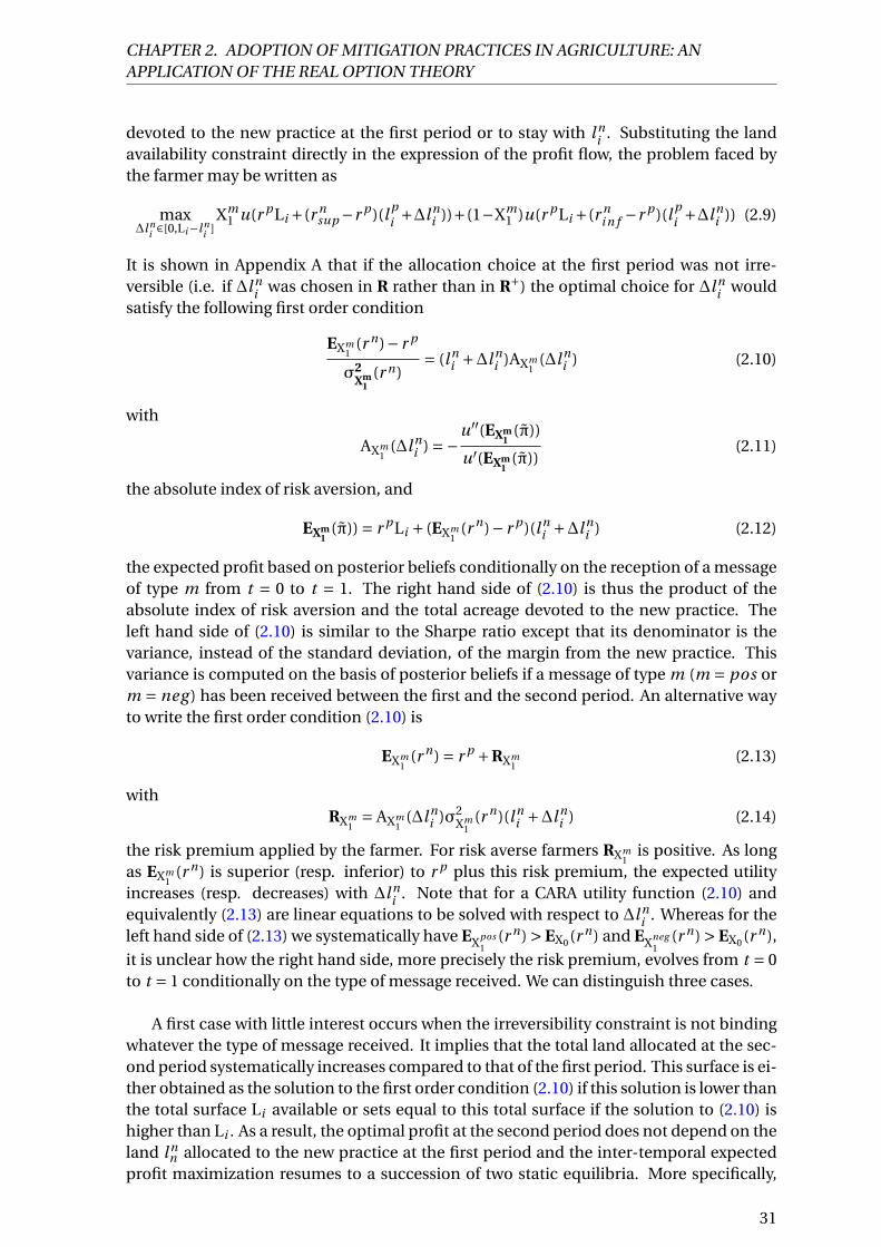
CHAPTER 2. ADOPTION OF MITIGATION PRACTICES IN AGRICULTURE: ANAPPLICATION OF THE REAL OPTION THEORY
devoted to the new practice at the first period or to stay with l ni . Substituting the land
availability constraint directly in the expression of the profit flow, the problem faced bythe farmer may be written as
max∆l n
i ∈[0,Li−l ni ]
Xm1 u(r p Li +(r n
sup −r p )(l pi +∆l n
i ))+(1−Xm1 )u(r p Li +(r n
i n f −r p )(l pi +∆l n
i )) (2.9)
It is shown in Appendix A that if the allocation choice at the first period was not irre-versible (i.e. if ∆l n
i was chosen in R rather than in R+) the optimal choice for ∆l ni would
satisfy the following first order condition
EXm1
(r n)− r p
σ2Xm
1(r n)
= (l ni +∆l n
i )AXm1
(∆l ni ) (2.10)
with
AXm1
(∆l ni ) =−
u′′(EXm1
(π))
u′(EXm1
(π))(2.11)
the absolute index of risk aversion, and
EXm1
(π)) = r p Li + (EXm1
(r n)− r p )(l ni +∆l n
i ) (2.12)
the expected profit based on posterior beliefs conditionally on the reception of a messageof type m from t = 0 to t = 1. The right hand side of (2.10) is thus the product of theabsolute index of risk aversion and the total acreage devoted to the new practice. Theleft hand side of (2.10) is similar to the Sharpe ratio except that its denominator is thevariance, instead of the standard deviation, of the margin from the new practice. Thisvariance is computed on the basis of posterior beliefs if a message of type m (m = pos orm = neg ) has been received between the first and the second period. An alternative wayto write the first order condition (2.10) is
EXm1
(r n) = r p +RXm1
(2.13)
withRXm
1= AXm
1(∆l n
i )σ2Xm
1(r n)(l n
i +∆l ni ) (2.14)
the risk premium applied by the farmer. For risk averse farmers RXm1
is positive. As longas EXm
1(r n) is superior (resp. inferior) to r p plus this risk premium, the expected utility
increases (resp. decreases) with ∆l ni . Note that for a CARA utility function (2.10) and
equivalently (2.13) are linear equations to be solved with respect to ∆l ni . Whereas for the
left hand side of (2.13) we systematically have EXpos1
(r n) > EX0 (r n) and EXneg1
(r n) > EX0 (r n),
it is unclear how the right hand side, more precisely the risk premium, evolves from t = 0to t = 1 conditionally on the type of message received. We can distinguish three cases.
A first case with little interest occurs when the irreversibility constraint is not bindingwhatever the type of message received. It implies that the total land allocated at the sec-ond period systematically increases compared to that of the first period. This surface is ei-ther obtained as the solution to the first order condition (2.10) if this solution is lower thanthe total surface Li available or sets equal to this total surface if the solution to (2.10) ishigher than Li . As a result, the optimal profit at the second period does not depend on theland l n
n allocated to the new practice at the first period and the inter-temporal expectedprofit maximization resumes to a succession of two static equilibria. More specifically,
31
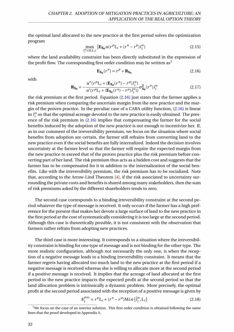
CHAPTER 2. ADOPTION OF MITIGATION PRACTICES IN AGRICULTURE: ANAPPLICATION OF THE REAL OPTION THEORY
the optimal land allocated to the new practice at the first period solves the optimizationprogram
maxl n
i ∈[0,Li ]
{EX0 u(r p Li + (r n − r p )l n
i ) (2.15)
where the land availability constraint has been directly substituted in the expression ofthe profit flow. The corresponding first order condition may be written as1
EX0 (r n) = r p +RX0 (2.16)
with
RX0 =−u′′(r p Li + (EX0 (r n)− r p )l ni )
u′(r p Li + (EX0 (r n)− r p )l ni ))
σ2X0
(r n)l ni (2.17)
the risk premium at the first period. Equation (2.16) just states that the farmer applies arisk premium when comparing the uncertain margin from the new practice and the mar-gin of the proven practice. In the peculiar case of a CARA utility function, (2.16) is linearin l n
i so that the optimal acreage devoted to the new practice is easily obtained. The pres-ence of the risk premium in (2.16) implies that compensating the farmer for the socialbenefits induced by the adoption of the new practice is not enough to incentivize her. If,as in our comment of the irreversibility premium, we focus on the situation where socialbenefits from adoption are certain, the farmer still refrains from converting land to thenew practice even if the social benefits are fully internalized. Indeed the decision involvesuncertainty at the farmer level so that the farmer will require the expected margin fromthe new practice to exceed that of the proven practice plus the risk premium before con-verting part of her land. The risk premium thus acts as a hidden cost and suggests that thefarmer has to be compensated for it in addition to the internalization of the social ben-efits. Like with the irreversibility premium, the risk premium has to be socialized. Notethat, according to the Arrow-Lind Theorem [4], if the risk associated to uncertainty sur-rounding the private costs and benefits is shared among many stakeholders, then the sumof risk premiums asked by the different shareholders tends to zero.
The second case corresponds to a binding irreversibility constraint at the second pe-riod whatever the type of message is received. It only occurs if the farmer has a high pref-erence for the present that makes her devote a large surface of land to the new practice inthe first period at the cost of systematically considering it is too large at the second period.Although this case is theoretically possible, it is not consistent with the observation thatfarmers rather refrain from adopting new practices.
The third case is more interesting. It corresponds to a situation where the irreversibil-ity constraint is binding for one type of message and is not binding for the other type. Themore realistic configuration, although not necessarily the only one, is when the recep-tion of a negative message leads to a binding irreversibility constraint. It means that thefarmer regrets having allocated too much land to the new practice at the first period if anegative message is received whereas she is willing to allocate more at the second periodif a positive message is received. It implies that the acreage of land allocated at the firstperiod to the new practice impacts the expected profit at the second period so that theland allocation problem is intrinsically a dynamic problem. More precisely, the optimalprofit at the second period associated with the reception of a positive message is given by
πpos1 = r p Li + (r n − r p )Mi n
{l n
i ,Li}
(2.18)
1We focus on the case of an interior solution. This first order condition is obtained following the samelines that the proof developed in Appendix A.
32

CHAPTER 2. ADOPTION OF MITIGATION PRACTICES IN AGRICULTURE: ANAPPLICATION OF THE REAL OPTION THEORY
with l ni > l n
i the solution to (2.13) for m = pos that makes πpos1 independent of l n
i . Con-versely, the optimal profit at the second period associated with the reception of a negativemessage is given by
πneg1 = r p Li + (r n − r p )l n
i (2.19)
and depends on l ni . The dynamic land allocation problem that the farmer is facing is then
maxl n
i ∈[0,Li ]
{EX0 u(r p Li + (r n − r p )l n
i )+β[PposEXpos
1u(πpos
1 )+Pneg EXneg1
u(πneg1 )] (2.20)
where the land availability constraint has been directly substituted in the expression ofthe profit flow of the first period. It is shown in Appendix B that the first order conditionassociated to this program is2
EX0 (r n) = r p +RX0 +βPnegu′(r p Li + (EXneg
1(r n)− r p )l n
i )
u′(r p Li + (EX0 (r n)− r p )l ni )
[(r p +RXneg1
)−EXneg1
(r n)] (2.21)
with RX0 the risk premium at the first period, defined in (2.17), whereas RXneg1
is the risk
premium, defined in (2.14) at the second period when a negative message has been re-ceived. Condition (2.21) highlights how the irreversibility premium and the risk premiumare combined in a non-additive way. The second term in the right hand side of (2.21) isthe risk premium associated to the first period and is formally identical to the risk pre-mium already defined in (2.17) and discussed in the first case where the irreversibilityconstraint is never binding. The third term in the right hand side of (2.21) is close to ir-reversibility premium obtained in (2.8) for the risk neutral farmer. It has a similar formexcept that i) the margin from the proven practice is corrected by the risk premium RXneg
1
before computing its difference with the expected margin EXneg1
(r n) from the new practice
and ii) the weight βPneg applied to the difference between the two margins is multiplied
byu′(E
Xneg1
(π))
u′(EX0 (π)) the ratio of the marginal utility of the expected profit at the second period
and the one at the first period3. We conclude that the total premium in (2.21) is the sum ofthe risk premium at the first period and the irreversibility premium corrected to accountfor risk aversion at the second period. This total premium has to be socialized if one wantsthat the hidden cost bear by the farmer vanishes. We provide a graphical example of thenegative adjustment of the level of adoption in t = 0 in Appendix C.
2.5 Endogenous learning process
So far, information has been treated as exogenous in the sense that farmers were bene-fiting from messages whatever the surface of land they collectively devoted to the newpractice. Such a context matches with the information provided by an agricultural re-search center but disregards all information produced by farmers themselves. This sec-tion thus turns to the case of farmers who self-produce information. It addresses thequestion of how to extend the model to this case of endogenous learning and induce fromthis adapted model the subsidy required to internalize the inherent informational exter-nality. A numerical illustration to the case of miscanthus in the French departement ofEure-et-Loire is also provided.
2We focus on the case of an interior solution for l ni .
3This feature can be interpreted as a level of aversion towards profits inequality over time.
33

CHAPTER 2. ADOPTION OF MITIGATION PRACTICES IN AGRICULTURE: ANAPPLICATION OF THE REAL OPTION THEORY
2.5.1 Information as a public good
The two key parameters influencing the learning process in the case of exogenous infor-mation examined supra are the probabilities θsup and θi n f associated to the reception ofrespectively a positive message if the correct scenario is the optimistic one (i.e. r n = r n
sup )and a negative message if the correct scenario is the pessimistic one (i.e. r n = r n
i n f ). These
two parameters capture the noise surrounding the reception of messages. A high value ofθsup (resp. θi n f ) means that there is a low degree of noise surrounding the reception ofa message when the correct scenario is the optimistic (resp. pessimistic) scenario. Goingback to equations (2.1) and (2.2), one easily checks that higher values of both θsup and
θi n f imply a more drastic change in the subjective likelihood ratioXm
11−Xm
1in t = 1 between
the two scenarios compared to the likelihood ratio in t = 0 whatever the type of receivedmessage (with an upward change if a positive message is received and a downward changeis a negative message is received). With endogenous learning, we assume that the degreeof noise depends on the scale of experiments of the new practice which is directly relatedto the total surface allocated to it at period t = 0 over all farmers. As a consequence, eachfarmer contributes to the production of information through the land she allocates to thenew practice, even if farmers are atomistic in the sense that they are too small to considerthat the land they will allocate individually to the new practice influences the learningprocess. Said another way, information is a public good that is unvoluntarily producedby atomistic farmers. The "production" of information is assumed to satisfy the law ofpositive but decreasing marginal returns in the sense that the θs are increasing and con-vex with respect to the total land allocated by farmers to the new practice. Formally, wecapture this idea by setting {
θsup (Ln) = 1−e−ln( 12 )−λsup Ln
θi n f (Ln) = 1−e−ln( 12 )−λi n f Ln (2.22)
with
Ln =∫
il n
i di (2.23)
As farmers are assumed to be identical in our model, this last term is equivalent to Ln =I∗ l n
i where I denotes the (high) number of farmers. According to (22), if no land is al-located to the new practice at period t = 0 then θsup = 1/2 and θi n f = 1/2 which in turnimplies according to (2.1) and (2.2) that the beliefs remain unchanged. This is consistentwith the fact that there is no information if no land is allocated to the new practice. At leasta small surface dedicated over all farmers to the new practice is required to experience itand learn form that experience. It also means that endogeneous learning is incompatiblewith risk neutrality. Indeed it has been shown supra that risk-neutral farmers individuallyopt for a all or nothing adoption strategy. Given that all farmers are identical according tothe assumption of symmetry, it induces that either all risk neutral farmers totally allocatetheir land to the new practice at the first period and the information produced is worth-less because of the irreversibility of adoption or all farmers do not allocate any acreage ofland to the new practice at the first period so that no information is produced, beliefs re-main unchanged and farmers have no new element to make them revised their decisionat the second period. By contrast, in the presence of risk aversion, farmers may chooseto allocate part of their land to the new practice, the exact surface involved being depen-dent of the amount of information anticipated and thus of the total amount of land thatswitches to the new practice at the first period. For i symmetric farmers, the amount of
34

CHAPTER 2. ADOPTION OF MITIGATION PRACTICES IN AGRICULTURE: ANAPPLICATION OF THE REAL OPTION THEORY
land individually allocated to the new practice is determined as a fixed point of the sys-tem formed by the solution in l n
i to program (2.20) for given parameters θsup = 1/2 andθi n f = 1/2 and the value of parameters θsup and θi n f obtained as the functions defined(2.22) and (2.23) of the acreage l n
i individually allocated to the new practice at the firstperiod. Prior detailing the numerical solution obtained for this fixed point in the case ofmiscanthus for the French department Eure-et-Loire in the next subsection, the internal-ization of the informational externality characterizing the case of endogenous learningdeserves some discussion.
With endogenous learning, each farmer contributes to the production of informationas a public good. This contribution is unintentional because farmers do not internalizedthe effects of this production on other farmers, besides the fact that there are atomisticand do not even consider their decision will affect the degree of information they willbenefit from at the second period. The surface of land they individually decide to allo-cate to the new practice is thus socially suboptimal. A subsidy to allocate more land tothe practice is thus required to make individual decisions match with the collective in-terest of farmers and this subsidy comes in addition to the payments discussed supra tosocialize the irreversibility premium combined with the risk premium. Contrary to thesepayments, the required subsidy results from cross informational externalities betweenfarmers and is conceptually more standard: the optimal subsidy per acre of land devotedto the new practice has to be fixed to a level corresponding to the marginal increase of theexpected discounted profit of each farmer at the first period that results from a marginalincrease of unit of the land devoted to the new practice when total land is fixed at itssocial optimum (i.e. when the informational externality is internalized). However, dueto the intricate impact of the total surface devoted to the the new practice on the opti-mal allocation choice of a farmer, we have to rely on numerical computation to asset theamount of subsidy required.
2.5.2 Numerical illustration
We simulate the farmers’ optimal acreage decisions and the values of irreversibility andrisk premia, and amount of subsidy for the internalization of informational externali-ties. We calibrate our numerical simulations with the data from Bocquého and Jacquet[7] about miscanthus and switchgrass adoption decisions by farmers in the French de-partment Eure-et-Loire. They provide real data about yields, output prices, subsidies andvariables costs for miscanthus, switchgrass and conventional crops, namely rape, winterbarley and soft wheat. We use these data for the calculation of the margins from con-ventional and uncertain crops. They also choose a discount rate of 5% and an absoluterisk aversion coefficient of 1,4.10−5. We focus on miscanthus and soft wheat as the con-ventional crop, the most cultivated crop in the studied region according to the publicagricultural census [2]. The utility function is assumed to be on the exponential form,u = 1−e−AΠ. We set:
r sup =e500/ha,
r i n f =e130/ha,
r p =e198/ha,
X0 = 0.33,
35

CHAPTER 2. ADOPTION OF MITIGATION PRACTICES IN AGRICULTURE: ANAPPLICATION OF THE REAL OPTION THEORY
Li = 100ha,
ρ= 0.05,
A =e−11,4.10−5,
I = 1000.
We assume that 1000 farmers choose the optimal level of adoption account beingtaken of the parameters and their choices are included in the computation of the θm
(2.22). The following results consider thus endogenous information. In this configura-tion, without irreversibility RX0 equals e37.7 per hectare and RX1 equals e5.1 per hectare.If we add irreversibility, the quasi-option value under risk neutrality equals zero, becausethe parameters are such that the expectations are high enough to induce adoption andthe farmer would not experience any regrets from adoption. Reversely, under risk aver-sion, the irreversibility premium equals e16.4 per hectare. In this case, the total premium(risk premium in t = 0 plus irreversibility premium under risk aversion) equals e54.1 perhectare. This is the value of the simulated marginal private costs that farmers have to bearif they adopt miscanthus on their farm under this set of parameters. This result is interest-ing because it shows that information has an impact also through the irreversibility effect(around e11 per hectare), and that, only with risk aversion. Under risk neutrality, thefarmer can’t have any regret from adoption, due to the fact that she will either not adoptat all (no information is generated), or adopt at 100% and irreversibility makes informa-tion not relevant. Under risk aversion, partial adoption by the farmers generates informa-tion per se, information which in turn impacts the positive irreversibility premium. Thecalibration allows us to compute the level of subsidy that is needed to compensate for themarginal value of the information externality generated by adopters: 15 cents per hectare,which is very low.
Without irreversibility, the adoption in t = 0 equals 100 hectares as expected (adop-tion is maximal), whereas it equals 88.9 hectares with irreversibility and risk aversion.This result presents a quantification of the impact of irreversibility and uncertainty withendogenous information on the level of adoption, and the adoption potential if the regu-lator chooses to hedge the simulated total premium. Around 11% of the theoretical levelof adoption in t = 0 is lost. It shows the partial adoption from the adjustment in the firstperiod. The theoretical static level of adoption in t = 1 in case of negative message (with-out irreversibility) equals 16.827 hectares under the values of the endogenous θs, whichis significantly under the level of adoption in t = 0 with irreversibility. It illustrates theimpact of negative signals and risk aversion, and the adjustment of the level of adoptionin t = 0 of the farmer who prevents herself from regretting a too high level of adoption.
2.6 Discussion
2.6.1 Implications
Diverse implications can be derived from our results. First, as we observed in the risk-neutral farmer’s part with exogenous information, beliefs play an important role in thewillingness to adopt, because they directly relate to the valuation of the different agricul-tural practices or activities’ profits and thus the opportunity for farmers to adopt or not(initial beliefs and updated beliefs). The comparison between certain profits and uncer-tain profits is a crucial part of the choice for farmers all along the model.
36

CHAPTER 2. ADOPTION OF MITIGATION PRACTICES IN AGRICULTURE: ANAPPLICATION OF THE REAL OPTION THEORY
A quasi real option value is associated to the presence of irreversibility, which leads tothe integration of the possibility to receive a negative message. In this situation, farmersweight their evaluation of comparative margins with what they forecast about the worstscenario they can fall in, and that, from the first period. Under risk neutrality, the weight-ing will only change the propensity to adopt because it can increase the adoption "trig-ger" that is necessary to exceed the status quo’s certain margin. This effect can decreaseincentives to adopt the uncertain practice, and adoption follows a "go-no go" scheme.The irreversibility premium can be considered as a hidden costs that can be socializedthrough a public compensation. A second hidden cost arise under risk aversion: a riskpremium appears at each period’s choice, that corresponds to an additive cost of adop-tion that prevent risk averse farmers from adopting. Partial adoptions can arise in thissituation because of interior solutions to the maximization program. Once again, the reg-ulator can hedge for this premium through a public compensation: it is equivalent to saythat a high number of tax payers share the risk instead of the private farmer. Finally, ifthe irreversibility is binding in case of negative message, and under risk aversion, choicesare not divisible over time anymore, and the total irreversibility premium corresponds tothe combination of a quasi-option value and a risk premium. This premium impacts thefarmer’s evaluation of margins and the related adoption choice from t = 0, and can limither willingness to make a diversification process on the farm, while most of the currentagricultural public policies aim per se at promoting diversification. These features impactadoption from the first period, which is a crucial result because it is directly related to thediffusion of innovations at the early stages (negative messages can "nip diffusion in thebud"). However, when information source is exogenously determined, it is impossibleto assess how farmers’ choices themselves can impact others adoption. A third hiddencost arises from the generation of informational externalities coming from adoption offarmers themselves. Because of our assumptions of homogeneity between farmers in thedepartment and irreversibility, information has no influence under risk neutrality. Re-versely, under risk aversion, partial adoptions induce information generation about themitigation practice and information externalities arise. In this scope, information can beconsidered as a public good which production as to be guaranteed with a subsidy thatencourage adoption on more land. The farmers-adopters must be compensated for theeffect of the information they produce when they adopt on the group and the fact theyhelp achieving the social goal.
We make a numerical illustration of these diverse hidden costs related to uncertaintyon the case of miscanthus planting. Miscanthus is a good instance of mitigation activitythat consists of a perennial fuel-crop whose yields are uncertain and fairly new for most offarmers compared to conventional crops. Our simulation relies on figures from the litera-ture. We show that in this case, the bigger hidden cost concerns the total premium underrisk aversion. This hidden cost refrains farmers from adopting, and we can say that theregulator could achieve good results if this privated cost would be socialized. This resulthighlights that the irreversibility significantly increases the costs associated to uncertaintyand that it must be taken into account in the incentives programs: the level of subsidiesmay have to be strongly increased compared to the usual computation in "certain uni-verse". Nevertheless, the level of the costs is related to the calibration we made in thissimulation. Other cases must be explored, and sensitivity tests must be implemented.
37
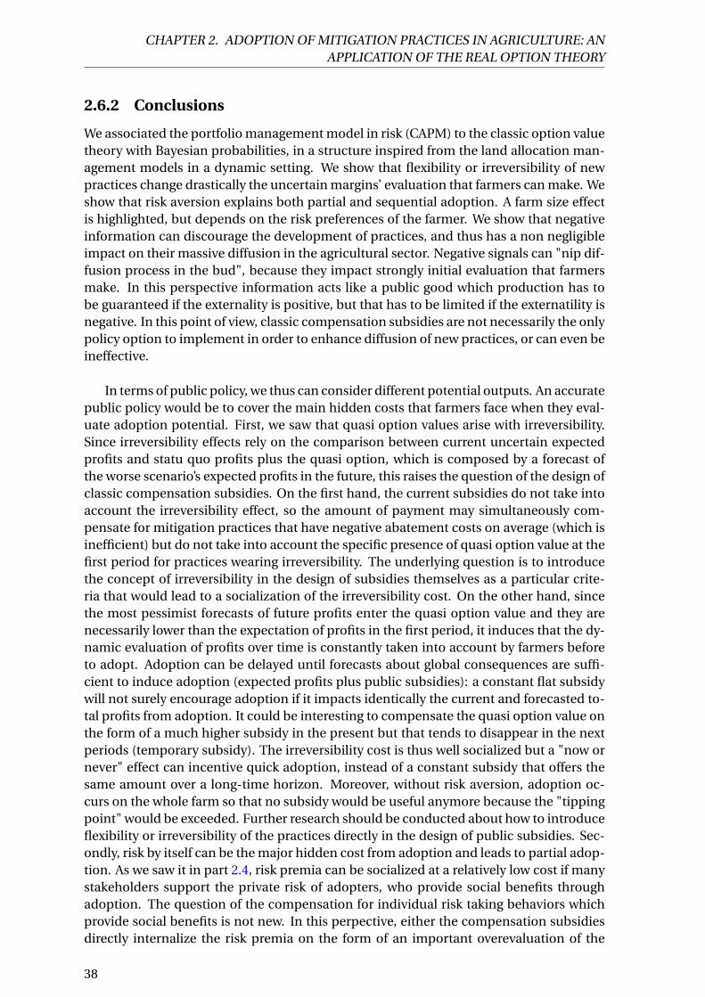
CHAPTER 2. ADOPTION OF MITIGATION PRACTICES IN AGRICULTURE: ANAPPLICATION OF THE REAL OPTION THEORY
2.6.2 Conclusions
We associated the portfolio management model in risk (CAPM) to the classic option valuetheory with Bayesian probabilities, in a structure inspired from the land allocation man-agement models in a dynamic setting. We show that flexibility or irreversibility of newpractices change drastically the uncertain margins’ evaluation that farmers can make. Weshow that risk aversion explains both partial and sequential adoption. A farm size effectis highlighted, but depends on the risk preferences of the farmer. We show that negativeinformation can discourage the development of practices, and thus has a non negligibleimpact on their massive diffusion in the agricultural sector. Negative signals can "nip dif-fusion process in the bud", because they impact strongly initial evaluation that farmersmake. In this perspective information acts like a public good which production has tobe guaranteed if the externality is positive, but that has to be limited if the externatility isnegative. In this point of view, classic compensation subsidies are not necessarily the onlypolicy option to implement in order to enhance diffusion of new practices, or can even beineffective.
In terms of public policy, we thus can consider different potential outputs. An accuratepublic policy would be to cover the main hidden costs that farmers face when they eval-uate adoption potential. First, we saw that quasi option values arise with irreversibility.Since irreversibility effects rely on the comparison between current uncertain expectedprofits and statu quo profits plus the quasi option, which is composed by a forecast ofthe worse scenario’s expected profits in the future, this raises the question of the design ofclassic compensation subsidies. On the first hand, the current subsidies do not take intoaccount the irreversibility effect, so the amount of payment may simultaneously com-pensate for mitigation practices that have negative abatement costs on average (which isinefficient) but do not take into account the specific presence of quasi option value at thefirst period for practices wearing irreversibility. The underlying question is to introducethe concept of irreversibility in the design of subsidies themselves as a particular crite-ria that would lead to a socialization of the irreversibility cost. On the other hand, sincethe most pessimist forecasts of future profits enter the quasi option value and they arenecessarily lower than the expectation of profits in the first period, it induces that the dy-namic evaluation of profits over time is constantly taken into account by farmers beforeto adopt. Adoption can be delayed until forecasts about global consequences are suffi-cient to induce adoption (expected profits plus public subsidies): a constant flat subsidywill not surely encourage adoption if it impacts identically the current and forecasted to-tal profits from adoption. It could be interesting to compensate the quasi option value onthe form of a much higher subsidy in the present but that tends to disappear in the nextperiods (temporary subsidy). The irreversibility cost is thus well socialized but a "now ornever" effect can incentive quick adoption, instead of a constant subsidy that offers thesame amount over a long-time horizon. Moreover, without risk aversion, adoption oc-curs on the whole farm so that no subsidy would be useful anymore because the "tippingpoint" would be exceeded. Further research should be conducted about how to introduceflexibility or irreversibility of the practices directly in the design of public subsidies. Sec-ondly, risk by itself can be the major hidden cost from adoption and leads to partial adop-tion. As we saw it in part 2.4, risk premia can be socialized at a relatively low cost if manystakeholders support the private risk of adopters, who provide social benefits throughadoption. The question of the compensation for individual risk taking behaviors whichprovide social benefits is not new. In this perpective, either the compensation subsidiesdirectly internalize the risk premia on the form of an important overevaluation of the
38

CHAPTER 2. ADOPTION OF MITIGATION PRACTICES IN AGRICULTURE: ANAPPLICATION OF THE REAL OPTION THEORY
current subsidies amount, or other risk management policies can be implemented likespecific insurance depending on the risk sharing characteristics associated to the farm-ers and the practices. Researches are currently conducted about this last point. Thirdly,information production coming from first adopters plays a role from the early stages ofnew practices’ diffusion. This public good’s cost is carried by the first adopters and re-lated benefits are shared by other farmers: a subsidy aiming at paying the first adoptersfor information production may be crucial to induce a mechanic motion of adoption anddiffusion among the agricultural sector.
39

CHAPTER 2. ADOPTION OF MITIGATION PRACTICES IN AGRICULTURE: ANAPPLICATION OF THE REAL OPTION THEORY
This research is part of the Agriculture and Forestry research program by the ClimateEconomics Chair. The authors want to thank the Climate Economics Chair for financial
support. The BETA contributes to the Labex ARBRE ANR-11-LABX-0002-01.
40

CHAPTER 2. ADOPTION OF MITIGATION PRACTICES IN AGRICULTURE: ANAPPLICATION OF THE REAL OPTION THEORY
Bibliography
[1] Just, Richard and Zilberman, David. Stochastic structure, farm size and technologyadoption in developing agriculture. Oxford Economic Papers, 1983. 25
[2] L’Evaluation et la Prospective Agricole Recensements agricoles Ministere del’Agriculture et de l’Alimentation Agreste, La Statistique. URL http://agreste.
agriculture.gouv.fr. 35
[3] Satheesh V Aradhyula and Matthew T Holt. Risk behavior and rational expectationsin the us broiler market. American Journal of Agricultural Economics, 71(4):892–902,1989. 25
[4] K Arrow. J. and RC lind. Uncertainty and Evaluation of Public Investment Decisions.American Economics Review, 60:364–78, 1970. 32
[5] Kenneth J Arrow and Anthony C Fisher. Environmental preservation, uncertainty,and irreversibility. In Classic papers in natural resource economics, pages 76–84.Springer, 1974. 24, 30
[6] Marc Baudry. Un modèle canonique d’option réelle bayésienne et son applicationau principe de précaution. Annales d’Économie et de Statistique, (89):91–119, 2008.26
[7] Géraldine Bocquého and Florence Jacquet. The adoption of switchgrass and mis-canthus by farmers: Impact of liquidity constraints and risk preferences. Energy Pol-icy, 38(5):2598–2607, 2010. 35
[8] Dennis R Capozza and Robert W Helsley. The stochastic city. Journal of Urban Eco-nomics, 28(2):187–203, 1990. 25
[9] Robert G Chambers and Richard E Just. Estimating multioutput technologies. Amer-ican Journal of Agricultural Economics, 71(4):980–995, 1989. 25
[10] Jean-Paul Chavas and Matthew T Holt. Acreage decisions under risk: the case of cornand soybeans. American Journal of Agricultural Economics, 72(3):529–538, 1990. 25
[11] Jean-Paul Chavas and Matthew T. Holt. Economic Behavior Under Uncertainty: AJoint Analysis of Risk Preferences and Technology. The Review of Economics andStatistics, 78(2):329, May 1996. 25
[12] Avinash K. Dixit and Robert S. Pindyck. Investment Under Uncertainty. PrincetonUniversity Press, 1994. 25
[13] Gershon Feder. Farm Size, Risk Aversion and the Adoption of New Technology underUncertainty. Oxford Economic Papers, 32(2):263–283, 1980. 25
[14] Gershon Feder. Adoption of interrelated agricultural innovations: Complementar-ity and the impacts of risk, scale, and credit. American Journal of Agricultural Eco-nomics, 64(1):94–101, 1982. 25
[15] Gershon Feder and Gerald T. O’Mara. Farm size and the diffusion of green revolutiontechnology. Economic Development and Cultural Change, 30(1):59–76, October 1981.25
41

CHAPTER 2. ADOPTION OF MITIGATION PRACTICES IN AGRICULTURE: ANAPPLICATION OF THE REAL OPTION THEORY
[16] Gershon Feder and Roger Slade. The acquisition of information and the adoption ofnew technology. American Journal of Agricultural Economics, 66(3):312–320, 1984.24
[17] Amir K. Abadi Ghadim and David J. Pannell. A conceptual framework of adoption ofan agricultural innovation. Agricultural Economics, 21(2):145–154, 1999. 25, 26
[18] Claude Henry. Investment decisions under uncertainty: the" irreversibility effect".The American Economic Review, 64(6):1006–1012, 1974. 24, 30
[19] M Isik, M Khanna, A Winter-Nelson, et al. Adoption of site-specific technologiesunder uncertainty. In Proceedings of the 5th International Conference on PrecisionAgriculture, Bloomington, Minnesota, USA, 16-19 July, 2000, 1–13. American Societyof Agronomy, 2000. 25
[20] Murat Isik and Madhu Khanna. Stochastic technology, risk preferences, and adop-tion of site-specific technologies. American Journal of Agricultural Economics, 85(2):305–317, 2003. 26
[21] Murat Isik and Wanhong Yang. An analysis of the effects of uncertainty and irre-versibility on farmer participation in the conservation reserve program. Journal ofAgricultural and Resource Economics, pages 242–259, 2004. 25
[22] Richard Jensen. Adoption and diffusion of an innovation of uncertain profitability.Journal of economic theory, 27(1):182–193, 1982. 26
[23] Richard E. Just and David Zilberman. The effects of agricultural development poli-cies on income distribution and technological change in agriculture. Journal of De-velopment Economics, 28(2):193–216, 1988. 25
[24] H Knight Frank. Risk, uncertainty and profit. The Riverside Press, 1921. 26
[25] Duncan Knowler and Ben Bradshaw. Farmers’ adoption of conservation agriculture:A review and synthesis of recent research. Food Policy, 32(1):25–48, February 2007.26
[26] Stefan Köppl. Real options for agricultural investments. Metody Ilosciowe w Badani-ach Ekonomicznych, 14(1):253–264, 2013. 25
[27] Yoram Kroll, Haim Levy, and Harry M Markowitz. Mean-variance versus direct utilitymaximization. The Journal of Finance, 39(1):47–61, 1984. 25
[28] Nicolai V Kuminoff and Ada Wossink. Valuing the option to convert from conven-tional to organic farming. Technical report, 2005. 25
[29] Howard D. Leathers and Melinda Smale. A Bayesian approach to explaining sequen-tial adoption of components of a technological package. American Journal of Agri-cultural Economics, 73(3):734–742, 1991. 24
[30] Haim Levy and Harry M Markowitz. Approximating expected utility by a function ofmean and variance. The American Economic Review, 69(3):308–317, 1979. 25
[31] Harry Markowitz. Portfolio selection. The journal of finance, 7(1):77–91, 1952. 25, 49
42

CHAPTER 2. ADOPTION OF MITIGATION PRACTICES IN AGRICULTURE: ANAPPLICATION OF THE REAL OPTION THEORY
[32] Giancarlo Moschini and David A. Hennessy. Chapter 2 Uncertainty, risk aversion,and risk management for agricultural producers. In Handbook of Agricultural Eco-nomics, volume 1 of Agricultural Production, pages 87–153. Elsevier, January 2001.25
[33] John von Neumann and Oskar Morgenstern. Theory of Games and Economic Behav-ior. Princeton University Press, March 2007. 30
[34] Rulon D. Pope and Randall A. Kramer. Production Uncertainty and Factor Demandsfor the Competitive Firm. Southern Economic Journal, 46(2):489, October 1979. 25
[35] T Jeffrey Price and Michael E Wetzstein. Irreversible investment decisions in peren-nial crops with yield and price uncertainty. Journal of Agricultural and Resource Eco-nomics, 173–185, 1999. 25
[36] Bharat Ramaswami. Production risk and optimal input decisions. American Journalof Agricultural Economics, 74(4):860–869, 1992. 25
[37] Atanu Saha. Risk preference estimation in the nonlinear mean standard deviationapproach. Economic Inquiry, 35(4):770–782, 1997. 25
[38] Agnar Sandmo. On the theory of the competitive firm under price uncertainty. TheAmerican Economic Review, 61(1):65–73, 1971. 25
[39] Paolo Sckokai and Daniele Moro. Modeling the reforms of the common agriculturalpolicy for arable crops under uncertainty. American Journal of Agricultural Eco-nomics, 88(1):43–56, 2006. 25
[40] David Sunding and David Zilberman. Chapter 4 The agricultural innovation process:Research and technology adoption in a changing agricultural sector. In Handbook ofAgricultural Economics, volume 1 of Agricultural Production, pages 207–261. Else-vier, January 2001. 26
[41] Abebayehu Tegene, Keith Wiebe, and Betsey Kuhn. Irreversible investment underuncertainty: Conservation easements and the option to develop agricultural land.Journal of Agricultural Economics, 50(2):203–219, 1999. 25
43

CHAPTER 2. ADOPTION OF MITIGATION PRACTICES IN AGRICULTURE: ANAPPLICATION OF THE REAL OPTION THEORY
44
Appendices
45


Appendix A
This appendix presents the optimal choice of a farmer at the second period given thatl n
i acres of land have been allocated to the new practice at the first period but there is noirreversibility. Let first define
ε= r n −EXm1
(r n) (24)
the difference between the realization of the margin of the new practice and its expectedvalue with posterior beliefs when a message of type m is received. Let also define
π= r p Li + (r n − r p )(l ni +∆l n
i ) (25)
the associated random profit at the second period.
We consider the following expected profit maximization problem:
max∆l n
i ∈[0,Li−l ni ]
EXm1
(u(π)) (26)
The associated first order condition for an interior solution writes
EXm1
(u′(π)r n)−EXm1
(u′(π))r p = 0 (27)
This first order condition is transformed in two steps. In a first step, the property Cov(x, y) =E(x y)−E(x)E(y) (and thus E(x y) = Cov(x, y)+E(x)E(y) is applied to (27). This yields
CovXm1
(u′(π),r n)+EXm1
(u′(π))(EXm1
(r n)− r p ) = 0 (28)
In a second step, it is assumed that ε is sufficiently small to enable the use of linear ap-proximation of the marginal utility in the vicinity of zero :
u′(π) ≈ u′(EXm1
(π))+u′′(EXm1
(π))(π−EXm1
(π)) (29)
It follows on that we may write
EXm1
(u′(π)) ≈ u′(EXm1
(π)) (30)
and, combining with the properties of the covariance
CovXm1
(u′(π),r n) ≈ u′′(EXm1
(π))CovXm1
(π,r n) (31)
Substituting the expression of π and using the notation σ2Xm
1(r n) = CovXm
1(r n ,r n) we can
also writeCovXm
1(u′(π),r n) ≈ u′′(EXm
1(π))(l n
i +∆l ni )σ2
Xm1
(r n) (32)
Accordingly, the first order condition becomes
u′′(EXm1
(π))(l ni +∆l n
i )σ2Xm
1(r n)+u′(EXm
1(π))(EXm
1(r n)− r p ) = 0 (33)
or equivalently
EXm1
(r n) = r p −u′′(EXm
1(π))
u′(EXm1
(π))σ2
Xm1
(r n)(l ni +∆l n
i ) (34)
47
Appendix B
This appendix presents the optimal choice of a farmer at the first period given thatl n
i acres of land can be allocated to the new practice and there is irreversibility (program2.20). Irreversibility is binding only in the case of the reception of a negative message.In this case, the acreage of land allocated at the first period is such that it impacts nega-tively the expected profits at the second period and the farmer would regret her allocationchoice.
We consider the following expected profit maximization problem:
maxl n
i ∈[0,Li ]EX0 (u(π))+β[PposEX
pos1
(u( ˜πpos1 ))+Pneg EX
neg1
(u( ˜πneg1 ))] (35)
The associated first order condition for an interior solution can be written
CovX0 (u′(π),r n)+EX0 (u′(π))(EX0 (r n)−r p )+βPneg [CovXneg1
(u′(π),r n)+EXm1
(u′(π))(EXneg1
(r n)−r p )] = 0(36)
The first order condition becomes
u′′(EX0 (π))l ni σ
2X0
(r n)+EX0 (u′(π))(EX0 (r n)− r p )+βPneg [u′′(EXneg
1(π))l n
i σ2Xneg
1(r n)+EXm
1(u′(π))(EXneg
1(r n)− r p )] = 0
(37)
or equivalently
EX0 (r n) = r p−u′′(EX0 (π))
u′(EX0 (π))σ2
X0(r n)l n
i +βPnegu′(EXneg
1(π))
u′(EX0 (π))[r p−
u′′(EXneg1
(π))
u′(EXneg1
(π))σ2
Xneg1
(r n)l ni −EXneg
1(r n)]
(38)
Appendix C
This appendix presents a graphical illustration of the adjustement in t = 0 due to irre-versibility and risk aversion. If we denote a the share of the portfolio that is at risk we canpose σXt (π) = aσXt (r n). Note that the first order condition in static (equation 34) can berewritten at time t
EXt (r n)− r p
σXt (r n)=−u′′(EXt (π))
u′(EXt (π))σXt (π) (39)
Where the left-hand side corresponds to a Sharpe ratio and the right-hand side corre-sponds to the product of the absolute risk aversion and the standard error of the profit.
For later purpose, we poseEXt (r n )−r p
σXt (r n ) = Jt . At this asymptotic point the farmer is indifferent
between profits expectation and risk, given that more risk must be remunerated by moreprofits. The arbitrage between risk and expectation is here, clear-cut, and allows for thedetermination of the optimal level of adoption l n∗
i . This result is close to the Capital As-sets Pricing Model rationale: the level of remuneration of the taken risk gives the slope ofthe risky asset demand, that corresponds to the Sharpe ratio. We will see later the graphi-cal illustration of that.
With irreversibility, we get back to equation (38), that can be written as a transforma-tion of the previous equation (39) on the form
48

J0 =−u′′(EX0 (π))
u′(EX0 (π))σX0 (π)−βPneg
u′(EXneg1
(π))
u′(EX0 (π))
σXneg1
(r n)
σX0 (r n)[Jneg
1 +u′′(EXneg
1(π))
u′(EXneg1
(π))σXneg
1(π)] (40)
The last feature between brackets on the right-hand side is equivalent to the first ordercondition in t = 1 in case of the reception of a negative message. At the optimum, it equals0 and equation (40) is equivalent to (39). If it is expected negative (which would normallyinduce "disadoption"), we know that the irreversibility can be binding, and it implies anadjustement of the level of adoption from t = 0. It is important to note that a featureσ
Xneg1
(r n )
σX0 (r n ) is added, which is a weighting component: we interpret it as a weighting of the
value of potential "regrets" in the second period from too much adoption by the relativeevolution of risk over time. If it equals 1, the farmer does not forecast that the risk willevolve over time and there is no impact on the level of adjustement. However, if the risk isassumed to increase between both periods, it is superior to 1 and the adjustement will bestronger. The interpretation is symmetric for the case of a decreasing evolution in the risk.
We can draw this result on Figure 1 as an example:
Figure 1 – Partial adjustement of adoption w.r.t. potential bad scenario - author. forecasts
This graph is similar to the Capital Asset Pricing Model rationale, whose assumptionsare closed to those of Markowitz [31]. The choice of the farmer is represented on a two-dimensions graph, with the level of portfolio risk on the x-axis and the portfolio profitsexpectation on the y-axis. The blue dashed line represents the risky asset demand curve.The level of adoption is catched on the x-axis, through the level of risk the farmer is readyto accept. The adoption is bounded by the total farm size Li : if adoption reaches thislevel, the taken risk is maximum. At the point 0 on the x-axis, the level of risk is null andthe farmer does not diversify at all: she only keeps the conventional practice. The bluedot represents the asymptotic point from equation (39) in t = 0. In this situation we as-sume that there is no binding irreversibility, and the level of adoption is given by l n∗
i . If
49
the irreversibility is binding in case of negative message, the farmer will adjust her levelof adoption from the first period, in order to not experience any regrets in the secondperiod. This mechanism can be understood as a displacement of the asymptotic point(orange dot) due to a decrease in the slope of the asset demand curve (dashed orangeline), simultaneous to an increase in the Arrow-Pratt "curve" with respect to the portfoliorisk (orange solid line), which can be understood as a transformed marginal rate of sub-stitution between each unit of risk and the level of profit expectation. The adjusted levelof adoption is given by l n∗∗
i .
50

Chapter 3
Yields volatility and friction in landconversion
Contents3.1 Introduction . . . . . . . . . . . . . . . . . . . . . . . . . . . . . . . . . . . . 52
3.2 Literature review . . . . . . . . . . . . . . . . . . . . . . . . . . . . . . . . . 53
3.2.1 Grassland potential in terms of mitigation strategy . . . . . . . . . . 53
3.2.2 Uncertainty in input production and sources of irreversibility . . . 54
3.2.3 Estimating the role of uncertainty in the producer choices with jointproductions . . . . . . . . . . . . . . . . . . . . . . . . . . . . . . . . . 55
3.3 Land allocation and uncertainty measures . . . . . . . . . . . . . . . . . . 57
3.3.1 Theoretical framework of land allocation and yields . . . . . . . . . 57
3.3.2 Measuring yields uncertainty . . . . . . . . . . . . . . . . . . . . . . . 59
3.4 Empirical application . . . . . . . . . . . . . . . . . . . . . . . . . . . . . . 62
3.4.1 Descriptive statistics . . . . . . . . . . . . . . . . . . . . . . . . . . . . 62
3.4.2 Computation of the uncertainty measures . . . . . . . . . . . . . . . 64
3.4.3 Econometric model . . . . . . . . . . . . . . . . . . . . . . . . . . . . 65
3.5 Results assuming exogeneity of explanatory variables . . . . . . . . . . . 66
3.5.1 Test for colinearity with time variables . . . . . . . . . . . . . . . . . 67
3.5.2 Regressions with below-above average yields variable . . . . . . . . 67
3.5.3 Regressions with volatility variables - without controls . . . . . . . . 68
3.5.4 Regressions with Volatility variables and controls . . . . . . . . . . . 68
3.6 Instrumental regression . . . . . . . . . . . . . . . . . . . . . . . . . . . . . 69
3.6.1 Limits of the exogeneity assumption . . . . . . . . . . . . . . . . . . 69
3.6.2 Instrumental (IV) regressions . . . . . . . . . . . . . . . . . . . . . . . 70
3.6.3 Results of IV regressions . . . . . . . . . . . . . . . . . . . . . . . . . . 71
3.7 Conclusion . . . . . . . . . . . . . . . . . . . . . . . . . . . . . . . . . . . . . 72
51
CHAPTER 3. YIELDS VOLATILITY AND FRICTION IN LAND CONVERSION
3.1 Introduction
The last decades are associated to the combination of simultaneous important issues inthe farming-breeding systems in France. Firstly, the importance of keeping sufficientrevenues to farmers, allowing them to produce enough, aiming to feed the populationand live their life in the same time, while continuing the investment in their farms inthe future. The sustainability of the crop and animal products’ production in economicterms is crucial, while the quick increase of the demand for meat and milk at a globalscale is challenging like never before. In a second time, the increasing preoccupationfor environment-related subject, especially climate change which is strongly impacted bythe agricultural sector (more than 20% in France in 2016 according to CITEPA [8]), ecosys-tems preservation and animal condition, highlights the importance of the way farmers arepracticing their activities. It is especially true concerning the farming-breeding systems,that relies on both animal feeding and animal products’ production, and is an impor-tant producer of greenhouse gases: CH4 through animal eructation and dejection storage,N2O relative crop production intended to feed the cattle and animal dejection use, andcarbon storage and flows related to the weight of land cover management related to thecrop production. Indeed, the forage crop, as a specific land cover (that is related to foragevegetable cropping, cereal and especially ensilage maize cropping, and grass productionthrough all the different kinds of grasslands) represents for itself 45% of the agriculturalsurfaces in France (Huyghe [19], TERUTI dataset). During the second half of the pastcentury, a significant part of grasslands has been destructed in order to produce foragecrops (especially cereals) because of higher productivity gains in these productions andhigher advantages in terms of CAP aids (ibid.). This phenomenon led to intense carbonleakages, while grasslands’ soils are able to store around 70-100tC/ha during a sufficientduration, which represents almost the same amount as forest soils (Arrouays et al. [3]).On the contrary, intensive annual cropping led to carbon losses and soils quality degra-dation (without taking into account the impact of cropping practices in terms of syntheticnitrogenous fertilization). Converting an annual crop into a permanent grassland is esti-mated to store 0.84 to 2.75 t eqCO2/ha/an (ibid.).
As a well-known public report highlighted, among the less costly and most potentiallymassive in terms of net GHG reduction mitigation practices, the grassland managementis one of the most interesting (Bamière et al. [4]). Indeed, two main measures amongthose which have the better reduction/cost ratio are related to grassland: the increase ofpasture duration (-e112/ha/year, around -e500/tCO2eq/year for an average farm) and ofthe temporary grassland duration (-e26/ha/year, around -e180/tCO2eq/year for an av-erage farm) wear a non-negligible reduction potential, and also have negative emissionunit abatement costs. The increase of the weight of pasture and/or grassland in the cattlefeeding management (the "forage mix") implies a mechanic increase of their weight in thecrop rotation. However, the capacity to adopt more grassland in the whole land portfolioof a farmer depends on the marginal opportunity cost of land relative to the production ofinputs. Because of the potential estimated negative abatement costs, we can expect thatthe average marginal profitability of adoption might be positive. But if hidden costs re-lated to uncertainty in the food production (and then risk of feeding interruptions), and itslack of reversibility, occur, one can ask for how much they impact the willingness to con-vert lands. Indeed, croping grasslands is complex and requires some specific knowledgefrom farmers, and the associated yields are significantly volatile. Uncertainty in yieldswould increase the shadow value of land use substitution and prevent farmer from in-
52
CHAPTER 3. YIELDS VOLATILITY AND FRICTION IN LAND CONVERSION
crease the extensive share of grasslands on their lands. This raises new questions: doesvolatility in yields lead to friction in land conversion toward grassland in the livestock sys-tem? What are the consequences in terms of public incentives policy? This preliminarystudy proposes a measurement of the elasticity of the use of each land-cover in livestock-oriented input production in response to uncertainty. A short land allocation frameworkis used, from which the empirical model is derived. An estimation on the French nationalterritory is performed on a balanced panel dataset with different measures of uncertaintyand different estimation strategies.
In Section 3.2, we made a literature review about the livestock-feeding systems (espe-cially grasslands) and the economic methodology that should be useful in our case. InSection 3.3, we present the land-allocation model and our constructed measures of yieldsuncertainty. In Section 3.4, we present the empirical specification, whose results are pre-sented in Sections 3.5, and 3.6 for the instrumental approach. Sections 3.7 is dedicated tocaveats and conclusions.
3.2 Literature review
3.2.1 Grassland potential in terms of mitigation strategy
According to the BANCO report (Bamière et al. [4]), lengthen the duration of temporarygrassland dedicated to graze production is a relevant mitigation: for an negative annualcost around e180/t.CO2eq for an average French breeder farm, it can achieve a carbonstorage of approximatively 1.3 Mt.CO2eq in the grasslands, that corresponds to a net ben-efit of around Me2.3 distributed among adopters. The GHG reduction potential is dueto two reasons, mainly the reduction plate (importance of this production in the agricul-tural sector), and the positive impact of the interrelated integration of herb product in theanimal feeding (good digestibility of herb) and the dejection management if animals arein pasture (more N2O by denitrification but less CH4 because of aerobic conditions and alot more C storage in the grassland). The negative abatement costs are related, accordingto the authors, to the compensation of potential loss of milk production in winter by thegains in terms of less soil work, less fertilizers costs, less ensilage and reaping work andcosts, less dejection spreading costs and less concentrated feeding use (ibid.). In terms ofcarbon storage in soils, estimations of grasslands’ significant potential have been imple-mented through the GES’TIM project (results are published in IDELE [20]).
The presence of negative costs is especially related to diminution of soil work andseedling preparation because the farmers do not have to sow and plant again the parcelannually (Bamière et al. [4]). However, the diffusion of this practice seems to be stableand not sustained, while the goal of the program “4 pour mille” is to increase the durationfor 99% of temporary grasslands by the year 2030. A shared objective of the governmen-tal program called "Zero Emission Nettes" (Zero net emmisions), which puts grasslandsin the center of its diverse carbon neutrality goal’s achieving tools. According to the re-port, some interviewed farmers evoked the fact that despite the possibility to decreasethe cost of cattle alimentation, it can increase their level of implication in the meadowsmanagement and it can be difficult to maintain good yields of graze production. It needs adeep reform of the exploitation management, and yields can decrease after the 4th year ofplantation. The complexity of the meadow management compared to a crop leads to thenecessity of having adapted skills, while the lengthening of meadows duration is related
53

CHAPTER 3. YIELDS VOLATILITY AND FRICTION IN LAND CONVERSION
to their raising part in the farm rotation (ibid.). Furthermore, farmers tend to secure theirgraze provision and are chilly towards changes that can potentially impact their yields atthe harvest. We can see that there are some barriers to adoption related to the intrinsicuncertainty about yields.
3.2.2 Uncertainty in input production and sources of irreversibility
Herb production is known as volatile with pedoclimatic conditions, and any mistake inthe grazing planning can lead to cattle-feeding risk (O’Shea et al. [28], Coléno and Duru[9]). In the same time, put back a land that is in annual forage crop production for instancerequires some changes in the practices: it is associated to specific skills and knowledgesabout herb production, while any big mistake in the grazing management can lead topotential losses (Bamière et al. [4]). In general, adoption of extensive as well as intensivechanges, or innovation, in agricultural activities are often associated to yields uncertainty,and can be related to risk taking or risk avoidance behaviors (Sunding and Zilberman [34];Ghadim and Pannell [16]; Knowler and Bradshaw [23]). We can expect that in a situationof uncertainty, farmers tend to seek information about the true value of yields before tomake any decision. Lybbert et al. [26] show that farmers use the forecast about extremeevent in order to update their beliefs about uncertain outcomes. In this situation, an op-tion value could arise and make it more costly to adopt the forage crop that has the higherlevel of uncertainty. The classic Expected Net Present Value (ENPV) models consider thatthe value of an asset (a non-vacant land in our case), that will explain its exploitation bythe owner, can be measured by the actualized net cash flow that she can expect from theexploitation. The farmer would thus compare the diverse usages she can deploy on herland and chooses the most profitable ones. But uncertainty can act like an implicit cost ifthe farmer values more the option to delay than the option to crop now, in order to avoidan investment in an asset whose true value of yields is difficult to forecast. We can con-sider in this situation that the shadow value of land cover, associated to the opportunitycost of forages crops, is distorted by yields uncertainty.
This problem has been questioned by Dixit et al. [11], as we see in the introductorychapter. If the returns from the new converted asset are uncertain and source of irre-versibility, the decision maker acts like for a “call” option product on the financial mar-ket. Regarding to her expectation about new asset’s returns and its irreversible cost, shecan choose or not to exercise now her option on the asset. If she does not want to lockherself in an uncertain asset or thinks she does not have enough information about theexpectable yields, she can postpone her option exercise and wait until favourable condi-tions seem to be gathered. If the “option value” raises above the present value of an asset,it is better to postpone the trade. The same rationale has been used in some works aboutland conversion and the result is that the conversion threshold can be increased by theuncertainty and irreversibility of new land use (Capozza and Li [6]; Plantinga et al. [30];Schatzki [33]; Cavailhès et al. [7]). This “option value” can explain some frictions in landconversion, by improving the estimation of the conversion thresholds and optimal tim-ing of croping, highlighting the limit of the “certain universe” model (ENPV). Basically,the land manager does not want to "lock" her land in a land-cover that is too uncertainbecause of the forecasts she can make about the value of production.
In another vein, the theory of decision under risk would explain the same type of fric-
54

CHAPTER 3. YIELDS VOLATILITY AND FRICTION IN LAND CONVERSION
tions in land allocation. Risk averse farmers would tend to adopt less of a productiontype if it is more spread around the expectation of yields. In this setting, the problem ofthe farmer corresponds to a portfolio problem under risk with an inclination toward lessrisky investments and a sufficient level of diversification in activities that do not covariate(Feder et al. [14]; Feder [13]; Just and Zilberman [22]). Diversification strategies thus arisedepending on the covariances between the yields of the different forage crops. We canexpect diverse drivers of the impact of the level of volatility in yields on the share of landdedicated to grassland.
Grasslands require some years before to be totally rentable, that causes inertia in theuse of the dedicated land. Moreover, in the specific case of permanent grasslands (+6years old), any tillage and replacement of it by other crops can lead to the suppressionof the "green payment" if it is not validated by the authority, that makes it irreversible ifnot. Annual forage crops do not wear these problems of combination of uncertainty andinertia, and farmers have tend to replace their herb production by more flexible annualcroping during a large part of the second half of the 20th century (Huyghe [19]). We thusassume that there can be an option value due to the association between uncertaintiesand irreversibility (or inertia) whose degree differ with the type of grassland. This is an in-teresting point that we will try to assess too, and it could be useful to compare the classicportfolio management approach from the option value approach. Indeed, risk premiumas well as option value can potentially explain why yields volatility can prevent farmersfrom croping a forage instead of another. But we assume that what can really differentiateherb productions, especially old-seeded grasslands from other, is the irreversibility or atleast intertia that it is related to, which can make farmers lock inside this type of land-cover if the grassland is more than 5 years old. The public regulation aiming at forbiddingtillage of permanent grassland presents the advantage of preserving the actual carbonstock, that is crucial. However, if it prevents farmers from adoption more extensively sus-tainable grassland in land rotations, it lowers the potential in terms of new carbon storage(i.e carbon sink). This work aims at explain by which canals this regulation can limit car-bon sink through grassland, and assume that uncertainty is a key issue. We do not claimthat we assess the impact of the regulation per se.
To conclude this part, we can say that switching the production from an activity intoa new one occurs when the relative returns between the two productions stand above aconversion threshold, from which the conversion brings to the farmers more expectedprofits than the past practice. The opportunity cost of a unit of land in a particular cover,that is related to its statistical marginal impact on final profits, equals the shadow price ofthis land-cover: it allows for accounting all the losses that can come from the substitutionfrom a cover to another (Bayramoglu and Chakir [5]). Yields uncertainty, empirically de-fined as the level of volatility of yields, can distort the shadow value of land-cover, makingit more costly to adopt the more volatile forage crops.
3.2.3 Estimating the role of uncertainty in the producer choices withjoint productions
Before to define more precisely how we will measure uncertainty, the first matter is tochoose a proper way to consider how uncertainty can play a role in the farmer’s profits.Two main ways of estimating the economic choice criteria for land-managers exist, and
55

CHAPTER 3. YIELDS VOLATILITY AND FRICTION IN LAND CONVERSION
their use depends on the case study.
The first is related to the ricardian rent measure, that considers that the value of a landcan be measured by the price of the land, because it integrates the net present value of allrevenues that it can provide to the owner (Capozza and Li [6]; Plantinga and Birdsey [29];Plantinga et al. [30]). The advantage of this approach is that it is tractable, in the sensethat the value of land on the market equals the sum of all the productive gross margins itis related to. The disadvantage is that it assumes an equilibrium and a perfect matchingbetween supply and demand that already met on the market, which is the reason why theprice gives all the information about gross margins. In our case, we study the research foran optimal set of land use inside a producer farm, and production arbitrage that can leadto conversion, destruction of forage land cover according to the extensive capacity of it.Moreover, we do not have a robust national dataset on grasslands prices or rent in Francefor each type of grasslands.
A second stream of land conversion studies is agricultural production economics’ mod-els: here the value of land depends on its capacity to produce a good that enters a profitprogram for the owner, profit which depends also on market prices for the good and pro-duction costs structure (Fezzi and Bateman [15]; Lacroix and Thomas [24]; Bayramogluand Chakir [5]; Moore and Negri [27]; etc.). Hotelling lemma shows that using a quasi-fixed input depends directly on the market price of the input or the per unit monetarybenefit it leads to (subsidy per ha for instance). The tension on lands (through a La-grangian multiplier) explains the repartition of lands in different productive land-covers.In our case, the second stream of studies looks more adapted to the management of cattle-feeding production by farmer-breeder. Indeed, our rationale farmers use annual foragecrops or grassland as joint-technology inputs that are then used for cattle-feeding, andthus output production (milk, meat especially). Their main production posts are animalproducts that they try to optimize, and in this purpose they manage the input mix in themost optimal way they can.
However, we face several specific features. First, a large part of the empirically tractablemodels in the agricultural productions’ economics (second stream) use a dual profit ap-proach (Fezzi and Bateman [15]; Lacroix and Thomas [24]; etc.). The optimization of prof-its in order to find optimal choices of output and input quantity, as well as fixed factorsuses, leads to estimate them through simultaneous equations related to the whole pricessystem. The econometric models are straightly related to this specification. In our case,we do not want the quasi-fixed factors (land allocation each year) to be only expressedthrough the market prices, but also through some input availability-related factors (yields’volatility expressed in diverse forms). Second, a difficulty that arises in our case is that theimpact of forage on profits is very indirect: it is related to the capacity of each forage togive value to animals and animal products through its level of digestibility and differentproduction costs (indirect multi-output technology), things that we can’t observe here atall1. Moreover, in our case study, the markets for inputs do not play their basic incen-tive roles: the majority of forages are produced and consumed entirely on the farm, inthe purpose of insuring input availability for the main production (animal products). Thefarmer seeks to have a good average forage production and the more stable as possible.We assume that she has an utility for yields that relies only on these two main compo-nents. While the preferences of the farmers for more or less volatile productions are not
1Especially because of a lack of data about these variables.
56

CHAPTER 3. YIELDS VOLATILITY AND FRICTION IN LAND CONVERSION
exactly known, we will catch the impact of uncertainty through the composition of landcovers in the forage mix (extensive effect). This composition being directly related to theshadow price of land associated to forage crops yields, that encompasses yields volatilityand we do not have to assume a specific form for preferences. Endogeneity problems willarise, that we will try to address in the empirical part later. Our land allocation model willthus use a mix of appropriate frameworks.
3.3 Land allocation and uncertainty measures
3.3.1 Theoretical framework of land allocation and yields
We assume a continuum of farmers (breeders) at the district level. We focus on the part ofthe farm dedicated to forages, where forage crops have to be allocated to lands. Assumingfor the moment that their characteristics are iid, we consider that the objective functionof a representative farmer can be observed and that the related production choices areadditive across the department. The farmer is endowed with an initial number of forageparcels L (Σl ), that we can sum to 1, and chooses at each period t the type of land-coverh that she will allocate on each parcel. Her final objective is to produce inputs in order tofeed her cattle. Different land-covers h are possible, h ∈ H. The forages are not directlyproduced in the purpose of selling them on the markets: they are entirely produced andconsumed on the farm for the cattle. However, there exists a limited market for forage(especially forage maize), and we will use the prices data we obtained from it: it gives apartial idea about how is valued marketable forage in regional markets. We have no costsdata for these kinds of production, so we will focus on forage crops yields. Thus, we as-sume that the farmer tries to manage the best way as possible the land she has at herdisposal, while taking into account the yields expectation and volatility.
The first step is the following. The rationale farmer looks forward to maximize hervalue function V for forage crops’ yields. At each period, the farmer allocates a foragecrop production to different parts of the total area of her farm, in order to maximize herutility V.
V(l1, ..., lh) = ∑h∈H
lhu(yh) (3.1)
u(yh) is the twice-differentiable utility function for the production and yh are theyields of each forage crop. We assume that the utility is the same for each type of crop,only yields attributes are different. We assume that the sum of the utility on each type ofcrop, multiplied by the share of land in each crop, equals the total utility on the farm. Wedo not specify any preferences for volatility here: we just assume that the whole utility ofthe farmer is given by the sum of utility of what she can harvest from each productions.In static-dynamic, the choice of lh is determined according to the maximization of theutility function for the whole farm. The constraint is related to the total land availability.
maxl1,...,lh
∑h∈H
[lhu(yh)], (3.2)
s.t.L ≥Σlh .
57

CHAPTER 3. YIELDS VOLATILITY AND FRICTION IN LAND CONVERSION
Note that the above constraint can be rewritten as 1 = ΣlhL with lh
L = Ph the share ofeach land cover in the forage mix of the farm. In this case, the yields would be normalizedby area. If we consider the Lagrangian of the objective function and the constraints, andlook for an optimization of the objective function in each lh , we find the following firstorder condition (FOC):
u(yh)−λ= 0,∀lh . (3.3)
Then, we can assume that the forage yields take the form yh = y(µ,σ)h where µ is themean of yields that the farmer can expect for each forage, and σ is a measure of yieldsvariability, both observed at each point in time. λ is the Lagrange’s parameter of the landconstraint and is associated to the possibility of recomposition of the forage mix in termsof quantity of land allocated to forages, or share of land allocated to the forage in thewhole mix ("cost" of the constraint). The allocation is directly explained by the opportu-nity costs between each forage production. We can add that at the equilibrium
δV
δl1= δV
δl2= ... = δV
δlH= λ, (3.4)
for each share of crops, because of the total land constraint that leads to the equaliza-tion of each marginal value on each land. This last equation sets that the relative valuefunction for each land cover explains the repartition of lands (allocation mix). It is ashadow price equation that tells us that the shadow price (or value) of each land undercover h depends on its relative marginal value on the farm. Finally, Ph is associated tou(yh) and the constraint.
According to the condition (3.3), we can expect that the constraint relative to the landallocation leads to a recomposition of the land covers that follows the evolution of yieldsin terms of expectation and volatility, the preferences of the farmers. The FOC tells us thatthere can be corner solutions for each lh : the farmer chooses to totally allocate a parcel ina cover, but it is the sum of each similar cover that gives, on the total farm L and accordingto the total value V, a share that can be different from 0 or 1.
This simple model just allows us to observe the relationship between the allocation-reallocation of a quasi fixed factor, land, and the stochastic yields. This allocation is like anosmotic process, where the value spreads across the different lands through the choicesof the farmer and according to the best valuation, that evolves over time. The hiddencosts or benefits from a higher yields expectation or a higher yields volatility modify theshadow price of land covers, and impact directly the allocation of lands to each type ofproduction. One can argue that the reallocation of land in the total land-forage mix de-pends on the extensive and intensive margins, and thus the physic capacities that farmershave to increase or decrease the level of cultivated (used) land. We answer that the landparameter lh is normalized to the total available land allocated each year to forage cropsin each department, that varies across time in our data. Thus the extensive capacity (orconstraint) is already taken into account in the model, and the rationale we adopt (rela-tive share of land by forage compared to one reference crop) allows to find the optimalallocation of lands ceteris paribus.
The second step is related to the option pricing equation (Hertzler [18]; Sandersonet al. [32], Dixit et al. [11]): the temporal evolution of u(yh) can be assumed to follow an
58

CHAPTER 3. YIELDS VOLATILITY AND FRICTION IN LAND CONVERSION
optimal process of the following "risk-adjusted" instantaneous utility function form ateach t :
δu
δyhµ(yh)+ 1
2
δ2u
δy2h
σ2(yh) = 0. (3.5)
Where µ(yh) is the first moment of the yields and σ(yh) is the second moment of theyields2. This equation tells us that the utility for yields evolves following the dynamicmotions of yields, whose value is known at each period. The impact of this stochasticvaluation on land covers choices is subsequent, following equations (3.3-3.4). We have toprecise a crucial element: we do not introduce the dynamic equation with time prefer-ences in this work. While it is not our question, we try to emphasize the role of evolutionof distribution about yields, through their level of stationarity and variability. Thus, themodel is a static-dynamic model: the decision is taken again at each period, taking intoaccount the new available information. We expect a direct marginal impact of yields mo-tions on land cover allocation through a function F
Ph = F(S(yh),Z). (3.6)
Where Z is a vector of exogenous variables that enter the decision process (especiallymarket prices and cattle size) and S is the vector of interest variables in terms of yieldsuncertainty. There exist an interior solution to the program (3.2) through (3.5) at eachperiod t . In the purpose to validate the proposition underlying equation (3.6), we haveto choose the way we measure the yields’ underlying stochastic processes. Time-varyingvariance indicators are relevant tools to catch variability of yields over time.
3.3.2 Measuring yields uncertainty
Uncertainty is related to the fact that all the information about true yields is not avail-able to the farmer. She does not know what exact value the stochastic yields can take oneach year, and they can be above or below the expected yields. This volatility (i.e. theway exogenous shocks can affect the yields) is observable in each period of time, andeach observation can be gathered to the global knowledge the farmer had about a yieldsdeterministic part (trend, relatively predictable) and degree of walk around these trends(random or unpredictable). A large number of empirical studies that aim at estimatingthe role of production uncertainty go through the well-known risk econometric approachà la Just and Pope [21]. This framework is well-suited for the case of output stochasticityprovoked by inputs use: a production function estimation is computed, where outputsare estimated by inputs, and the heteroskedasticity subsequent to the estimation is con-sidered as a proxy for the level of risk. It is considered as a good proxy of risk becauseit is directly associated to the uncertainty about the results from a specific input and thedistribution of errors associated to an observable distribution of state-of-the-nature bythe farmer. This approach is related to the mean-variance specification of productionrisks. In our case, we do not want to precise the role of an input in the land cover choice,we aim at observing the global level of uncertainty of outputs. We do not need to seespecifically how an input can increase or decrease the level of volatility in ouput produc-tion. The source of uncertainty is assumed to be exogenous and totally exists per se, butis observable by farmers. It can be directly measured on our yields dataset, under the
2We go further in the explanation of these elements in Section 3.3.2.
59

CHAPTER 3. YIELDS VOLATILITY AND FRICTION IN LAND CONVERSION
strong assumption that all farmers in each department can access the same information.However, as we will see later, we suppose an endogeneity issue between our dependentvariables and our uncertainty variables, and we will test an approach that looks like theJust and Pope approach to tackle this issue. We propose different measures of uncertainty.
Below-Above the average yields
In a first attempt to measure the moves of the yields around the mean, we compute ameasurement relative to the deviation of yields of each crop around their long run aver-age within each department (Deschênes and Greenstone [10]). We calculated the distri-bution of yields of each type of interest forage for each district, then separated the yieldsat each period with a dummy variable that tells if they are in the first third, the secondthird (around the mean) and the third third in the yields distribution. The first category isconsidered as years with bad yields (negative shock), while the third one can be consid-ered as year with very good yields (positive shock). This measure is based on a probabilitydistribution that is not time varying. The advantage of this measure is that it is a straightway to calculate shocks (fluctuation), understood as the position of yields in their knownprobability distribution. The disadvantage is that this measure does not really representsthe dynamic evolution of gathered knowledges by the farmer. Indeed, it does not sepa-rate a long run trend that would be perceived by farmer as deterministic and a randomstochasticity of yields, that add knowledge step by step through shocks.
Yields’ stochastic motions
The Dixit et al. [11] measures of uncertainty (Brownian motion and mean-reversion espe-cially) are relevant in order to catch that stochastic motions-like phenomenon, becausethey rely on different interesting properties. First, they follow the Markov property, whichimplies that the future value of yields that can be forecasted each period only depends onits value in the current period. The consequence is that only the current available infor-mation plays a role in order to forecast the value of yields in the next period. No otherinformation at the same period will modify the value of yields, which implies that theuncertainty is measured through an incremental value that follows the periodic shocksthat percuss yields per se across time. The nature of the exogenous shocks are not speci-fied in this setting. When the farmer observes the current value of yields, it thus gatherspure information about how the yields are moving and can deviate from the deterministicforecast. This type of time-varying uncertainty measures were already used in the Black-Scholes-Merton type of models, describing the value of financial options with stochasticasset prices following a Wiener process3. Indeed, these models of uncertainty have es-pecially been used for asset price forecasts’ estimations, more than for commodity pro-duction forecasts. We have to precise that the low stepback in time that we have in ourdata (28 years, that corresponds to 27 degrees of freedom) would lead to potential biasesin the estimation of the uncertainty parameters. We compute the measure of uncertaintyby applying the calculus of standard deviation to the yields at each period and using thepast values of yields. We did that in the rest of the article, which has the advantage of be-ing stricly in correspondance with the theory, but bears the cost that the first calculatedvalues of the standard deviations are biased.
3Most of the literature using this approach assumes constant conditional variance and geometric Brow-nian motion processes.
60

CHAPTER 3. YIELDS VOLATILITY AND FRICTION IN LAND CONVERSION
The Brownian motion allows to express the dynamic motion followed by the yieldsthrough the equation (see Schatzki [33] for the below equations):
d y =µd t +σdW
Where µ is the instantaneous first moment (or expected growing rate or trend), σis the instantaneous standard deviation of the variable and W is a Wiener process withE(dW) = 0 and Var (dW) = d t . σ can be constant but its level updated with informationaccumulation, and describes an increasing variability across time (Postali and Picchetti[31]). This kind of motion is well-suited for commodities market prices’ stochastic pro-cesses. The subsequent measure of volatility is given by:
σBrt = ΣT−1
t=0 (yt − yt−1)2
t
1/2
(3.7)
However, for stationary variables whose stochastic value tends to revert toward themean after experiencing shocks, the Brownian motion specification could overestimatethe level of volatility and the subsequent forecast about the volatility. Indeed, if the vari-able looks like it tends to revert to a long run average and oscillate around it, the fact to seethe stochastic motion as totally unpredictable is biased because in reality agents have abetter possibility to forecast the moves of the variable across time. As we show in section3.4.1, every test we performed shows that our yields data are stationary. In these cases,several specifications are relevant.
The Ornstein-Uhlenbeck (OU) measure is suited for mean-reverting motions. Thesubsequent measure of uncertainty takes the form:
σOUt = νΣ
T−1t=0 (yt − y)2
t
1/2
(3.8)
Where y is a historical mean of yields (or long-run average) that we calculated on eachdepartment’s time serie, and ν is a parameter of mean reversion, that gives the speed ofreversion of yields toward the long run mean. We can also assume that the trend is notconstant on the long run and that the farmers update their beliefs about it, which can becatched through a moving trend at each period. The moving average (MA) measure lookslike the former on but the mean that is taken into account is moving at each period: itdoes not consider the long run "historical" mean, but an updated mean across time. Thesubsequent measure of uncertainty takes the form:
σMAt = ΣT−1
t=0 (yt − yt )2
t
1/2
(3.9)
Where yt = ET−1t=0 (yt ) is the moving-average of yields, updated at each period, that we
calculated on each department’s time serie.
Schatzki [33] used these three types of uncertainty measures in his article and foundvery different results for his estimation of option values for forest conversion. In this arti-cle, the author attributed to Ornstein-Uhlenbeck measures an arbitrarily fixed ν= 0.25 forall the sample. We assume that the level of reversion toward the long-run mean is properto each district. According to the Euler-Maryuama discretization of the Ornstein Uhlen-beck process at time t, the parameter νmust be estimated through an AR(1) estimation ofyields, on the form:
61

CHAPTER 3. YIELDS VOLATILITY AND FRICTION IN LAND CONVERSION
∆yt = a +byt−1 +εt (3.10)
With εt a white noise, and ν=−log (1+b) (Postali and Picchetti [31]).
3.4 Empirical application
3.4.1 Descriptive statistics
We have a panel of forage crops yields and land allocation for 96 French metropolitan dis-tricts, from 1989 to 2017 (Agreste [1]). For each year, we are able to calculate the sharelh of land in each type of forage crops (cereals or diverse types of grasslands) in the to-tal of lands dedicated to forage in the agricultural sector, with lh ∈ (0,1) (see Table 3.1).For the whole country, the weight of managed herb production in the total forage systemis around 70%4. An important thing to note is that the average share of land allocatedto each production is not straightforwardly related to the level of yields of each produc-tion: for instance, forage maize seems not to have a huge land share across departments(around 8%). However, the average yields related to maize are much higher than herbproductions in absolute terms because the production is far more intensive. The pro-ductivity by itself certainly explains the division of land in each production: while marketeffects migh poorly impact the cropping behaviors for forages, the most productive cropcan be cropped on smaller scales. Most of the standard deviations in shares of land in thedistricts sample are especially following a between effect, indicating that there are mostlydifference in the shares’ movements across the sample, rather than within each district.It can be the sign of an heterogeneity of geographical-based characteristics that drive theland-management, as well as local specialization and other fixed effects characteristics.
The average productivity is really diverse concerning herb productions, and probablyrelated to the level of implication and management of farmers: while the most permanentgrasslands seem to have low productivity and to lower the level of global herb productiv-ity, grasslands related to real cropping management by farmer (artificial and temporarygrasslands) have much higher productivities. Within variations as well as between varia-tions in yields are quite important for each production. However, they are not compara-ble in this form because they are associated to a “scale” of productivity in terms of volumethat can hide the true level of variation.
4Some grasslands are natural and low productive, in mountains for instance, and are not considered as“managed” with farming practices even if they are part of the total forage system.
62

CHAPTER 3. YIELDS VOLATILITY AND FRICTION IN LAND CONVERSION
Table 3.1 – Descriptive statistics
Variable (country level) Mean Std. Dev. Min Max Observations
Share in forage and silage maize overall .0831697 .0809431 0 .3456755 N=2431between .0795635 0 .3147234 n=95within .0176908 -.1188234 .2061766 T-bar=25.5895
Share in managed grassland overall .6841905 .2544402 0 1 N=2445between .241909 .0785267 .9854867 n=95within .0604501 .0175238 1.314501 T-bar=25.7368
Share in artificial grassland overall .0359801 .05417 0 .5961298 N=2445between .0678475 0 .5667724 n=95within .0170901 -.0365148 .1467519 T-bar=25.7368
Share in temporary grassland overall .1576005 .1361225 0 .5439466 N=2445between .1306143 0 .4828511 n=95within .0366858 -.0046349 .4379916 T-bar=25.7368
Share in non-permanent grassland overall .1935806 .1435085 0 .6147128 N=2445between .1419873 0 .5837825 n=95within .0345016 .0516038 .4961859 T-bar=25.7368
Share in natural or old-seeded grassland overall .4906098 .2514303 0 1 N=2445between .2450163 .0686073 .9537782 n=95within .0546118 -.1760568 .9022583 T-bar=25.7368
Forage maize yields (100kg/ha) overall 108.9248 27.36707 0 400 N=2343between 18.71835 45 153.2018 n=94within 21.48015 23.01569 419.8813 T-bar=24.9255
General herb yields (100kg/ha) overall 46.30722 21.24689 0 114.8 N=2443between 19.29617 8.097857 96.83182 n=95within 10.26511 -10.48385 94.35865 T-bar=25.7158
Artificial grassland herb yields (100kg/ha) overall 82.1444 21.97608 8.98 160.5 N=2398between 17.03947 45.47643 127.9227 n=94within 14.966 9.964042 156.3265 T=25.5106
Temporary grassland herb yields (100kg/ha) overall 67.91604 18.56736 0 139 N=2394between 13.87018 37.27321 104.43 n=94within 13.27152 -7.621107 122.6518 T=25.4681
Natural and old seeded grassland herb yields (100kg/ha) overall 46.90751 16.83583 0 110 N=2437between 13.60912 9.961538 79.26364 n=95within 10.58169 1.390366 98.94597 T-bar=25.6526
As we show in the previous part, there are different ways of measuring the level ofuncertainty in yields depending on the characteristics of the variables of interest and theobjective of the researcher. A crucial point to explore before to choose the proper mea-sure is the level of stationarity of the yields: it tells us if the yields tend to come back tothe mean after experiencing a shock. We use different tests in order to observe the levelof stationarity of our panel and use the appropriate expression of the subsequent process(Postali and Picchetti [31]). These tests show the (non) stationarity of department-widepanel variables (for yields of maize and all types of herb). In our case the interest variablesbeing non strongly balanced, the Fisher-type test of unit root was the more relevant. Thenull hypothesis is that the variable has a root that equals 1 with its lagged values. H1 con-siders thus that at least one panel is stationary, which means a parameter lower than onefor the lagged value, thus past shocks have a transitory effect on the variable (it followsa certain degree of stationarity), which tends to go back to the mean if there is a mean-reversion or moving-average process. We specified those tests for our yields in the case ofmaize, temporary grassland, artificial grassland, natural and old-seeded grassland and all
63
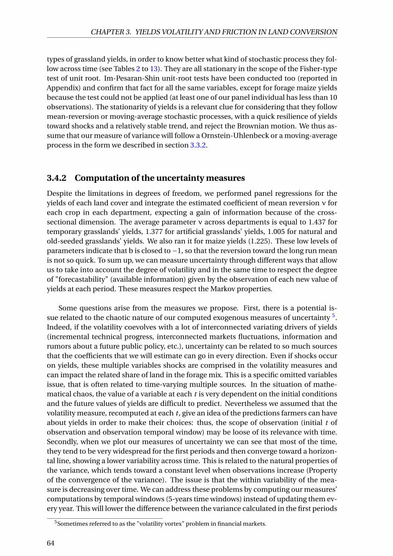
CHAPTER 3. YIELDS VOLATILITY AND FRICTION IN LAND CONVERSION
types of grassland yields, in order to know better what kind of stochastic process they fol-low across time (see Tables 2 to 13). They are all stationary in the scope of the Fisher-typetest of unit root. Im-Pesaran-Shin unit-root tests have been conducted too (reported inAppendix) and confirm that fact for all the same variables, except for forage maize yieldsbecause the test could not be applied (at least one of our panel individual has less than 10observations). The stationarity of yields is a relevant clue for considering that they followmean-reversion or moving-average stochastic processes, with a quick resilience of yieldstoward shocks and a relatively stable trend, and reject the Brownian motion. We thus as-sume that our measure of variance will follow a Ornstein-Uhlenbeck or a moving-averageprocess in the form we described in section 3.3.2.
3.4.2 Computation of the uncertainty measures
Despite the limitations in degrees of freedom, we performed panel regressions for theyields of each land cover and integrate the estimated coefficient of mean reversion ν foreach crop in each department, expecting a gain of information because of the cross-sectional dimension. The average parameter ν across departments is equal to 1.437 fortemporary grasslands’ yields, 1.377 for artificial grasslands’ yields, 1.005 for natural andold-seeded grasslands’ yields. We also ran it for maize yields (1.225). These low levels ofparameters indicate that b is closed to −1, so that the reversion toward the long run meanis not so quick. To sum up, we can measure uncertainty through different ways that allowus to take into account the degree of volatility and in the same time to respect the degreeof "forecastability" (available information) given by the observation of each new value ofyields at each period. These measures respect the Markov properties.
Some questions arise from the measures we propose. First, there is a potential is-sue related to the chaotic nature of our computed exogenous measures of uncertainty 5.Indeed, if the volatility coevolves with a lot of interconnected variating drivers of yields(incremental technical progress, interconnected markets fluctuations, information andrumors about a future public policy, etc.), uncertainty can be related to so much sourcesthat the coefficients that we will estimate can go in every direction. Even if shocks occuron yields, these multiple variables shocks are comprised in the volatility measures andcan impact the related share of land in the forage mix. This is a specific omitted variablesissue, that is often related to time-varying multiple sources. In the situation of mathe-matical chaos, the value of a variable at each t is very dependent on the initial conditionsand the future values of yields are difficult to predict. Nevertheless we assumed that thevolatility measure, recomputed at each t , give an idea of the predictions farmers can haveabout yields in order to make their choices: thus, the scope of observation (initial t ofobservation and observation temporal window) may be loose of its relevance with time.Secondly, when we plot our measures of uncertainty we can see that most of the time,they tend to be very widespread for the first periods and then converge toward a horizon-tal line, showing a lower variability across time. This is related to the natural properties ofthe variance, which tends toward a constant level when observations increase (Propertyof the convergence of the variance). The issue is that the within variability of the mea-sure is decreasing over time. We can address these problems by computing our measures’computations by temporal windows (5-years time windows) instead of updating them ev-ery year. This will lower the difference between the variance calculated in the first periods
5Sometimes referred to as the "volatility vortex" problem in financial markets.
64

CHAPTER 3. YIELDS VOLATILITY AND FRICTION IN LAND CONVERSION
(with a low number of years so a low stepback, which leads to a high potential bias) andthe variance computed with cumulated observations, and it adjusts for real forecasts thatfarmers can do with information they gather in the few past years. Moreover, it can ad-dress a part of the "volatility vortex" problem previously mentioned: allowing for volatilitymeasurement by temporal windows can filter for interconnected time-varying trends andshocks’ impacts. These measures can be interesting in order to observe what can be theshort scope uncertainty impact, and they allow us to add time fixed effects to our panelregression without taking the risk of yield highly biased estimates. We will use both ba-sic volatility measures and the same volatility measures recomputed by 5-years windowsin our estimations. We also estimated the marginal impacts of time-dummies for eachyear on our volatility measures, in order to observe the strength of statistical relationshipsof our measures with time (Table 14). Our moving-average measure by 5-years windows(MAW) for each department then take this form:
σMAWi t =
Σt−5k=t (yk − yk )2
5
1/2
(3.11)
Where yk = Et−5k=t (yk ) is the yields average recalculated for each temporal window. It is
more complex in the case of the Ornstein-Uhlenbeck measure because it is theoreticallyassociated to short-term fluctuations around the long-run average. In its basic form σOU
i t ,the OU measure can be embedded in the "volatility vortex" problem because the dynamicof the measure is connected to each yt . We computed an Ornstein-Ulhenbeck measureby windows (OUW) equals to the average fluctuation of the average yields by windowsrelative to the long-run average, on the following form:
σOUWi t = ν
Σt−5k=t (yk − y)2
5
1/2
(3.12)
Where y still the historical mean of yields. To sum-up, we have four different measuresof volatility: σOU
t the time-varying fluctuations around the long-run (historical) averageyields; σOUW
t the 5-years windows-varying fluctuations around the long-run (historical)average yields; σMA
t the time-varying fluctuations around the moving-average (recom-puted at each t) average yields; σMAW
t the time-varying fluctuations around the moving-average (recomputed for each 5-years windows) average yields.
3.4.3 Econometric model
Based on Hardie and Parks [17], and Ahn et al. [2] we use a linear logistic probabilitymodel specification. This model considers that the estimated relative shares of land ineach cover are like the conditional probability to withdraw a land cover in the sample,given the independent variables that we have about each land cover (and a reference landcover) characteristics. If the static estimated proportion of land in use h is given by Pi h
and we denote x the vector of all explanatory variables and β the vector of parameters toestimate, we can write Pi h in the following form:
Pi h = eβi h .x
1+ ∑h∈H−1
eβi h .x(3.13)
This ensures for the estimated shares of land covers to lay between 0 and 1. The ex-planatory variables are related to the land cover optimal choice model that we expressedin section 3.3.1 (interest variables plus other exogenous explanatory variables). Our first
65

CHAPTER 3. YIELDS VOLATILITY AND FRICTION IN LAND CONVERSION
linear estimation model is directly associated to equation (3.6). The logistic specificationlinks the conditional probability to observe the relative share of a land cover to a referenceland cover that plays the role of a common forage substitution option and a good com-parison point: we assume that ensilage maize is a relevant reference forage crop, becauseit is the intensive alternative option for substitution in cattle feeding compared to all thediverse herb-related forage systems for which we assume a particular uncertainty issue.Thus, we assume that Pi ht = li ht
li mt. The estimation model is expressed as:
Pr ob(li ht ) = ln(Pi ht ) = β0 +βh .xi ht −βm .xi mt + fi +εi t (3.14)
Where m is for ensilage maize, the reference forage crop, i is the district, βs are theparameters to estimate for the intercept and our variables of interest, fi represents dis-trict fixed effects and εi t is the error term. βm is constraint to be equal to 0 for a correctidentification of the model. District fixed effects are straightforward in our setting, dueto the important role that can play each district’s fixed characteristic that we can’t controlfor, in the estimation of the dependent variable. Moreover, we controlled for potentialheteroskedasticity and serial correlations in each estimation by computing a weigthingmatrix of correction à la White [35] and provide heteroskedasticity consistent standarderrors estimations. The final linear model takes the following form:
ln(Pi ht ) = β0 +β1h .Si ht +β2h .Zi ht + fi +εi t (3.15)
3.5 Results assuming exogeneity of explanatory variables
We have two control variables at our disposal. The first one is the selling price index ineach department for forage. As we said in section 3.2.3, the impact of this price is notclear-cut: markets for forage are not like usual markets, and we can’t expect farmers-breeders to behave in the usual way. Nevertheless, because forages are inputs that are pro-duced and consumed on the farm, if the price of ensilage maize for instance, increases, itwill incentive farmers to produce more of it. Indeed, selling on the market is more attrac-tive, and buying it is less attractive so it can incentive farmers to produce more by them-selves and self-consume more of it. Furthermore, this price index is essentially composedwith the price of ensilage maize. We can expect that its marginal impact on the relativeshares of land dedicated to grasslands is negative. The second control variable is a spa-tialized index for animal costs, that is a constructed proxy for the unit cost of bovines.Bovines are the main animal that farmers-breeders use to produce meat and milk, whichare the two main productions from animals in France. Raw data for animal price in eachdepartment are only accessible by region (RICA dataset) and not for each department. Inorder to introduce spatial variability in the index at the department level, we weight eachregional price index by a representative variable of the weight of the production volume ineach department (following Lewbel and Pendakur [25] kind of index). We obtain a com-posite index, that is a good proxy of the bovines buying cost in volume per year, wherevariability is catched through the variation in volume. We accessed data about the cattlesize (bovines) for each department per year. Overall our index is a factor of the regionalprice index for buying bovine and the share of bovine lifestock in the department relativeto the national lifestock. We expect this variable to be a good proxy for intensive costsof production, since the price of an animal integrates its production cost as well as thestream of value-added it can lead to. The regulation of grasslands in France and Europe
66

CHAPTER 3. YIELDS VOLATILITY AND FRICTION IN LAND CONVERSION
followed straighly the CAP reforms. As it is a key explanation for variations in grasslandsallocation, we can be tempted to ran regressions with time effects: it allows for catchingthe effect of policies that were homogeneously applied on all the country over time, andthus the impact of public policies, that is likely to be non-negligeable. However, we foundhigh levels of colinearity between our uncertainty measures and time dummies, whichcan lead to strong multicolinearity biases in our final estimations. This phenomenon isprobably related to the fact that our time-varying uncertainty measures have a significantdynamic nature and structurally depend on past periods.
We ran the regressions for three types of land covers: Temporary grasslands and Ar-tificial grasslands (land covers supposed to be less perennials or non-permanent), andNatural or old-seeded grasslands (land covers supposed to be totally perennials or per-manent)6. The old-seeded grasslands correspond to grasslands older than 6 years. Theresults are different according to the type of uncertainty measure and between both typesof forage. We regressed our dependent variables on the measures of yields fluctuationbelow-above average measures (section 3.3.2) and on the measures of volatility (section3.3.2). We ran Hausman post-estimation tests for all regressions: departement fixed ef-fects are validated for all regressions. Our results are thus with department fixed effect.We will only comment the significant coefficients (minimum confidence level: 10%). Ourregression is in log-level, thus the coefficients are in percentage. However, while coeffi-cients can be surprisingly high or sometimes low, they correspond to a level of averagerelative elasticity, and the total impact depends on the value of the independent variableand the value of the dependent variable (ratio of land) for individual observations. Due toformat issues, the results for regressions with control variables are split in distinct tablesfor each type of grassland. We provide the Fisher tests of global significance for all ourregressions and the R-squares. All the results are available in the appendices.
3.5.1 Test for colinearity with time variables
The Table 14 in appendix shows the estimated marginal impact of time dummies for eachyear on our volatility measures. The goal of these regressions is to assess the potentialmulticolinearity of time effects and uncertainty measures that can emerge in the main re-gressions. Not only individual covariates’ coefficients are important, but the level of globalsignificance of regression through Fisher p-value (last row) and the explanatory power ofregression with R-squared. It is interesting to note thatσOUW
TG ,σOUWAG andσOUW
NOS are not co-linear with time dummies, contrary to all the classic OU measures: it can be the sign thatthe goal of computing uncertainty measures by temporal windows in order to fix chaosin the volatility has eventually been achieved. Note that σMAW
TG is disconnected to time-effects too. These results show that in our panel regression, when we will add time fixedeffect to catch purely time-varying exogenous processes, we will avoid multicolinearitybias for these four variables.
3.5.2 Regressions with below-above average yields variable
We regressed the ratio of land in each type of grasslands by our categorical variables ofyields shocks for each type of grass. Positive or negative shocks are the categories that weconsider in the regressions, with the 2nd category as the reference variable. We also madeestimations with the lagged value of this shocks variable (t −1). Tables 15 to 17 are naive
6All the regressions have been ran with Stata 12.1r.
67

CHAPTER 3. YIELDS VOLATILITY AND FRICTION IN LAND CONVERSION
regressions by type of shocks on grasslands’ yields. Table 18 show regressions of all theshocks together on the three types of grasslands. We add ensilage maize shocks in theseregressions, in order to try this new control and see the relationship with the reference"asset" represented by maize.
Tables 15 to 18 presented in Appendix lead to the following summary result:
Result 1: Positive shocks on Natural and old-seeded grasslands’ yields seem to be as-sociated with a global persistent positive impact on adoption of all types of grasslands(relative to maize). It can be the sign that the yields of the most massive share of grass-lands in the whole grasslands in the country (NOS) is a global indicator of the good yearsfor herb production, and the willingness to develop herb systems (role in terms of infor-mation). Negative shocks on Temporary grasslands’ yields seem to lead to a contractionin the other types of grasslands on the short-run. We also shows a clear substitution di-versification strategy between Artificial grassland and ensilage maize.
The estimations of yields’ shocks impacts on grasslands adoption are limited becausethe shocks do not catch real time-varying uncertainties (stochastic motion) and they sup-pose perfect uniform information access over time. They present the advantage of givinga first idea of the role of stochastic deviations on land-use decisions.
3.5.3 Regressions with volatility variables - without controls
Tables 19 to 24 presented in Appendix lead to the following summary result:
Result 2: OU measures show a relatively robust negative impact on Temporary grass-lands’ ratio, while positive for Artificial grasslands’ ratio. MA measures always show apositive (but weakly robust) impact on Temporary and Artifical grasslands’ ratios. Time-effects always affect the results and make coefficients not significant anymore, except inthe case of OU measures by 5-years windows for Temporary grasslands, which is con-firmed with time fixed effects.
3.5.4 Regressions with Volatility variables and controls
Tables 25 and 26 presented in Appendix lead to the following summary result:
Result 3: Only basic yields’ volatility indicators for Temporary and Artificial grasslandsare robust when we add controls. The impacts of control variables are, for their part, rela-tively robust: the selling price index for forage always displays a highly significant negativeimpact on the ratio of land dedicated to grasslands, while the spatialized index for animalcosts displays a positive impact in the case of Temporary and Natural and old-seededgrasslands.
Results 1 to 3 are interesting in two manners: firstly, they show that fluctuations aretaken into account by farmers in their portfolio management. We observe some inter-actions between land covers and the yields shocks, and trade-offs between forage landcovers. They allow us to have a measure of the marginal impact of volatility across timeon land cover allocation, that corresponds to the elasticity of land cover allocation withrespect to uncertainty. However, these results show diverse degrees of robustness, which
68

CHAPTER 3. YIELDS VOLATILITY AND FRICTION IN LAND CONVERSION
especially raise questions about potential endogeneity issues.
We also may have a potential omitted variable: the covariance between yields of differ-ent forages. For instance, if the the volatility of herb yields in temporary grasslands is highbut negatively covariates with other type of forage production, farmers may tend to adoptit more in order to diversify their portfolio, thus insuring themselves against shortages.We catch it in our regression of yields shocks from maize yields and grasslands yields.The results show diverse portfolio allocation strategies in terms of risk and productionefficiency. The first effect looks like a diversification-specialization strategy: farmers al-locate lands in crop that do no covariate in order to insure their feeding capacity. Themore maize and artificial grassland (legume crops) yields will covariate, the less it is in-teresting for them to adopt both on the farm (specialization). The role of diversificationas a self-insurance is clear in this situation (see Just and Zilberman [22]). The second ef-fect shows a different phenomenon. The more Natural and old-seeded grasslands andTemporary grasslands (mix of classic gramineous and sometimes legume crops) yieldswill covariate, the more farmers will adopt both: in this situation diversification is not arisk management strategy. If ensilage maize and gramineous are perceived by farmersas complementary (and not substitute), more covariance is good because a variation inthe yields of one crop gives informations about how can evolve the other. This informa-tional learning effect is the other explanation of diversification strategy that is not directlyrelated to risk management but related to improvement in the accuracy of prediction ofyields (Ghadim and Pannell [16]).
Finally, it is likely that there are some endogeneity biases that reduce the accuracy ofour estimations. Indeed, some variables probably explain simultaneously the choice ofland covers and the yields (farmers’ average ability, lands characteristics, etc.), and theformer maybe explains the later (precedent crop effect, etc.). The farmer tries to optimizeevery posts of production on her farm at the same time, that can lead to omitted variableand simultaneity bias. We also observed the impact of adding time fixed effects. In or-der to correct that biases, we want to perfom an IV regression where our yields would beinstrumented by a totally exogenous variable. The weather seems to us as a straightfor-ward solution: indeed, meteorological shocks are totally exogenous, explain a large partof yields variability, and we can expect that they are exogenous from the dependent vari-able because the potential effect they could have on land use choice goes directly throughthe yields.
3.6 Instrumental regression
3.6.1 Limits of the exogeneity assumption
We assumed until now that our independent variables of interest were exogenous and thatthe estimated marginal impacts, catched through coefficients βh , were unbiased. This as-sumption is quite strong: variables that we didn’t introduce in the model can simultane-ously impact dependent and independent variables. First, the volatility of yields can gothrough multiple sources, proper to the farmers and their behaviors, that can explain theland cover choices too: abilities, distribution of lands in term of quality, diverse farmingstrategies and objectives, can be endogenous to both dependent variables and volatilityvariables. These variables are omitted in our model. Secondly, land covers choices can
69

CHAPTER 3. YIELDS VOLATILITY AND FRICTION IN LAND CONVERSION
explain a part of the actual yields at the end of the croping campaign, and both variablesare probably embedded in a productive cycle that can lead to simultaneity biases. Thebias can be written in the general form that follows:
δPh
δzi ht= β1h + δεi t
δzi ht(3.16)
This bias can be either positive or negative and lead to significant fallacies. A firststrategy used to tackle this bias is to use a lag operator of the endogenous explanatoryvariable. The endogenous variable is estimated with its lagged values. The error termsare assumed to be not autocorrelated in order to respect the Gauss Markov theorem. Anissue arises in our case: we cannot assume that there are no autocorrelation over timebetween our error terms because all the elements that impact our uncertainty variablesover time can still have an impact in t , then the estimated coefficient may not be BLUEanymore7. Another common methodology that allows to tackle this endogeneity issue isinstrumentation with an exogenous variable. We follow this strategy in this section. We donot presuppose a bias with certainty, but we want to hedge against all the possible fallaciesin order to provide robust results. We provide post-estimation tests for endogeneity foreach regression.
3.6.2 Instrumental (IV) regressions
Meteorological data are the natural exogenous variables that we focused on. Indeed, theyare totally exogenous and we assume that they strongly impact yields. Moreover, we as-sume that if they could have an impact on land use, it wouldn’t be outside of yields: theimpact of meteorological shocks on land allocation to forage crops can only go throughyields and how they are impacted by them. We gathered meteorological data from MeteoFrance by town by day from 1990 to 2017. They mainly consist of data about precipita-tions, temperature, level of humidity, evapotranspiration, and minimum and maximumtemperatures. We computed the mean and standard deviation of these variables per yearfor each city. Then, we average these variables by department by attributing each town toits department. We thus balanced our panel with aggregated meteorological data whichare assumed to be homogeneously distributed within the spatial units (we assume a po-tential aggregation bias). The vector of meteorological variable is denoted I.
An instrument is considered as good if it is strongly correlated with the instrumentedvariable and not much correlated with the error terms. For each dependent and inde-pendent variable, we selected the instruments by computing pairwise correlation matri-ces between each variable, then trying to find the best regressions as possible. We keeponly variables which are relevant (i.e. correlated with the endogenous variables), and forwhich pairwise correlations were significant at the 10% level. Coefficients are comprisedbetween −1 and 1. Our protocole is the following, and has been determined with respectto the limits of what our dataset was able to provide: first, we selected the instruments(meteorological variable) that yield a pairwise correlation coefficient (in absolute terms)higher than 0.20 with the endogenous variables. If we did not find such coefficient, wetried instrumentation with the most correlated meteorological data. We also prioritizedvariables that yield a pairwise correlation coefficient (in absolute terms) lower or equalto 0.10 with the dependent variables. However, we also tested instruments which can
7Best Linear Unbiased Estimator.
70

CHAPTER 3. YIELDS VOLATILITY AND FRICTION IN LAND CONVERSION
have a higher level of correlation with these dependent variables, because of our assump-tion that the impact goes essentially through yields. We added instruments, if necessary,and dropped some of them, in order to catch the best estimation results. This is why forfew instrumental regressions, the most correlated meteorological variable is not our finalchoice, if another strongly correlated variable yield better regression result, after control-ling for good fit of the instrumentation obviously. We thus have selected specific instru-ments for each volatility variable.
The resulting models are two-stage least-squares (2SLS) generalization of fixed-effectspanel-data regressions with instrumentation, of the form:
ln(Pi ht ) = β0 +βIVh . ˆSi ht +β2h .Zi ht + fi +εi t
ˆSi ht = β′0 +β3h .Ii ht +β4h .Zi ht +ε′i t
Where the second step is estimated first, and the subsequent estimates are introducedin the first step. For each regression, we computed an endogeneity post-estimation test(Sargan Hansen-Hausman test). If the test is significant, then the uncertainty variable isvalidated as endogenous because H0 poses that the variable is exogenous. We also com-puted an underidentification test (Kleibergen-Paap LM statistic) that tests if the instru-ments are sufficiently good in the first step. The null hypothesis is that we have under-identification, so we have to reject it in order to validate the instrumentation. We alsopresented overidentification test (Sargan Hansen J stat) for which the null hypothesis isthat the instrumental equation is not overidentified, so our 2SLS is validated if H0 is notrejected. Finally, we show the Fisher tests for each regression is order to observe the levelof global significance of each model. Sometimes our R-squared are negative, that is not aproblem in terms of significance of the estimation, but highlights some big caveats aboutthe explanatory power of the estimation.
3.6.3 Results of IV regressions
We only estimated IV regressions for the cases that we selected according to the protocoledescribed in section 3.6.2 (if a correct instrument is available). Thus, as we did not findany good instrument in our criteria for the moving average uncertainty measure for Tem-porary grasslands and Natural and old-seeded grasslands, we do not have regressions forthem. If the tests aiming at observing the goodness of the instruments were not validated,we made again the estimation while changing the instruments, until we yield the best re-sults. We will only comment the significant coefficients (at least 10% of significance) andthe regressions that have been validated in terms of instrumentation (see section 3.6.2)and global inference (last rows of tables 29 and 30).
Tables 27 and 28: We provided the results of correlations coefficient matrix betweenour volatility measures and the diverse aggregated meteorological variables we gathered.The star indicates a 10% significance level. The final instruments that we selected appearin bold.
Tables 29 and 30 presented in Appendix lead to the following summary result:
71

CHAPTER 3. YIELDS VOLATILITY AND FRICTION IN LAND CONVERSION
Result 4: The negative impacts of σOUTG and σOUW
TG on the Temporary grasslands’ ratiois confirmed. The negative impact of σMA
AG and the positive impact of σOUAG on the Artificial
grasslands’ ratio is confirmed. We show that our diverse measures of volatility imply di-verse results on Natural and old-seeded grasslands.
Our regressions yield very low R-squared in most of the cases. We also found neg-ative R-squared in some of our instrumental regressions. It shows that our estimationsometimes has a low explanatory power in terms of summed squared estimation errors.However, the global (Fisher tests) or local (student-t by variable) levels of our estimationswere most of the time very high. The main explanation of the negative R-squared is thatthe instrumental panel regressions with fixed effects do not yields the constant covariate(intercept) estimation, unlike the basic fixed effects panel regressions for which Stata at-tributes average value of the fixed effects. In this scope, we please the readers to focusmore on the Fisher global tests of significance.
Summary of main results: The regressions with yields shocks of the different typesof forages show some degrees of diversification strategies between forage in the "foragemix". While maize and artificial grasslands seem to be "stochastically" substituable, per-manent grasslands and non-permanent grasslands seem to be "stochastically" comple-mentary. The OU volatility impact negatively temporary grasslands ratio and positivelyarticifial grasslands ratio, but the more robust impact is associated to the OU measurenegative impact on temporary grasslands ratio, even with our measures by 5-years win-dows and with time fixed effects. The MA volatility presents the reverse results: the im-pact is positive for temporary grasslands ratio and negative for artificial grasslands ratio.These main results are relatively robust to control variables for basic volatility measures(not those by 5-years windows). Before IV regressions, we can say that the level of volatil-ity globally impact non-permanent grasslands ratios. Instrumental regressions generallyconfirm them and also show new impacts on permanent (natural and old-seeded) grass-lands ratio. Volatility measures (OU as well as MA) present a very strong positive impact,while the MA measure by 5-years windows present a negative impact on the permanentgrasslands ratio. This can be the sign of a strong endogeneity (stronger than for otherregressions) that were hiding real impacts of yields volatility.
3.7 Conclusion
We developed a short land cover allocation model and a related econometric model in or-der to explain the impact that can have yields uncertainties on the forage mix in France.We developed different measures of uncertainty, from a basic assumption of shocks alongthe yields distributions, to average fluctuations measures in line with the stochastic vari-ables motions’ theory (à la Dixit et al. [11]).
Shocks on natural and old-seeded grasslands’ yields seem to provide information about"herb" yields and impact the allocation of all kinds of grasslands. Some diversificationstrategies have been identified between complementary grasslands. The general propo-sition of these results is that complementarity or substitution between crops in terms ofstochasticity has to be taken into account if the regulator wants to enhance grasslandadoption in rotations. Grasslands have to be an "interesting option": farmers-breederstend to secure their forage yields, and thus try to manage their forage production follow-ing the yields volatilities and covariations between them. It also reinforces the evidences
72

CHAPTER 3. YIELDS VOLATILITY AND FRICTION IN LAND CONVERSION
that it is necessary to incorpore uncertainty in dynamic croping plan decisions modelling,which aims at improving simulation models (Dury et al. [12]).
Uncertainty measured as volatility (variability) of yields has diverse impacts accordingto the way we calculated it. But it is clear that it seems to impact more non-permanentgrasslands ratio relative to maize. Ornstein-Uhlenbeck uncertainty measures especially(related to a long-run average assumed to be known by the farmer) show a behavior ofavoidance for adoption of Temporary grassland. This particularly sounds like a real optionbehavior, associated to the aversion of farmers to lock themselves in Temporary grass-lands that can become permanent after 5 years, and can’t be destroyed. Prohibiting thereplacement of old-seeded grasslands may lead to less and less adoption of temporarygrassland, and artificial grassland to a lesser extent. However, our diverse measures some-times provided very different results when we assume exogeneity of the independent vari-ables: it is due to some limits that we partly address with instrumental regressions. Mostof the time, OU measures have a negative and relatively robust marginal impact on Tem-porary grasslands’ ratios. Forbidding the tillage of old grassland is well-suited for the con-servation of existing carbon stocks. But it interacts with the carbon flows in grasslandsif it prevents farmers from creating new grasslands, which are huge carbon sinks. Thisarbitrage between carbon sink and stock in grassland and the policy assessment must beaddressed with ex ante and ex post public policy evaluation methods.
Yields uncertainties impact the opportunity costs of land covers, sometimes positivelyand sometimes negatively, but mainly non-permanent grasslands. First observation, onecould assume that these diverse effects are related to the difference between our uncer-tainty measure: the OU measure is associated to variability around the long run mean,while moving-average, variability around the short run mean. It could have an impacton the role that play each measure in the forecastability of yields: the first one would berelated to long run strategies and adaptation to external conditions in general, while thesecond one would be more related to year-to-year adjustment to secure the livestock’sfeeding with local adjustments. Second observation: option value is associated to a situ-ation of uncertainty with irreversibility of adoption; however without irreversibility, it isdifficult to infer a specific behavior from farmers, who can tend to love this uncertainty oravoid it (depending on their preferences and beliefs).
Our work present some caveats. The first caveat is related to our micro-economicland-allocation model: it neither relies on ricardian rent theory (widely used), nor oneconomics of agricultural production models of land use (with dual profits function). Weattempt to make a clear model of static-dynamic choices combining uncertainty in aninstantaneous utility functional form and optimal land use choice in a utility maximiza-tion. This allows to stay general in terms of mathematical results and expectation in termsof empirical results, thus we do not have to specify preferences or a form for the utilityfunction. Moreover, the way forage markets work do not follow the usual input marketsassumptions (there is a high level of self-consumption), and the utility between forageproduction and animal production is not completely separable for all farmers: it wouldbe interesting to go farther in this direction. Also, we make strong assumptions to go fromthe micro-level to the department-aggregated model, and when we choose not to intro-duce any time preferences. Finally, we observe extensive margins, because we assume wecan control for most of intensive margins through our cattle-size spatialized index in theregressions with controls (section 3.5). It is still a possible additional limit of the model.
73

CHAPTER 3. YIELDS VOLATILITY AND FRICTION IN LAND CONVERSION
We assume that intensive margins are already optimally developed. A second caveat isthat there is an intrinsic limit in the assumption of constant conditional variance, essen-tially because the forage yields present leptokurtotic distributions in our sample (samelimit as in the Black-Sholes (B-S) models, that aims at providing optimal option pricing).In the B-S case, the value (or price) of an option or an asset is conditional to the value of itsunderlying asset (the distribution is thus conditional). This model fits perfectly optionsmarkets, especially if the distribution is also assumed to be conditional to past shocks(stochastic persistance of shocks on the financial markets). In our case, we do not lookat conditional variance per se, we look at the totally exogenous variability or volatility ofyields. Moreover, our volatility measures are not constant over time because they are up-dated each year. Another caveat is associated to the fact that the linear logistic economet-ric specification in the form we used it can require that we perform all regressions in thesame time (SUR model) in order to tackle simultaneity of land-cover allocation choices.We tried it with naive regressions but the estimations were computationaly very costlyand it was almost impossible to add any control variable or time effects. It would be inter-esting to go farther in this direction in another work. Finally, the choice of ensilage maizeas the reference crop relies on ad hoc assumptions: we did not test for the relevance ofthis choice. This crop also has been choosen because data on maize were available.
74

CHAPTER 3. YIELDS VOLATILITY AND FRICTION IN LAND CONVERSION
Bibliography
[1] Ministère de l’Agriculture et de l’Alimentation Agreste: La Statistique l’Evaluation etla Prospective Agricole. Recensements Agricoles. Statistique Agricole Annuelle. 62
[2] S. Ahn, A. J. Plantinga, and R. J. Alig. Predicting future forestland area: a comparisonof econometric approaches. Forest Science, 46(3):363–376, 2000. 65
[3] D. Arrouays, J. Balesdent, J.-C. Germon, P. Jayet, J. Soussana, P. Stengel, and D. Bu-reau. Contribution à la lutte contre l’effet de serre (stocker du carbone dans les solsagricoles de France?). Expertise Scientifique Collective, INRA, Paris, 2002. 52
[4] Sylvain Pellerin and Laure Bamière and Denis Angers and Fabrice Béline and MarcBenoit and Jean-Pierre Butault and Claire Chenu and Caroline Colnenne-David andStephane De Cara and Nathalie Delame and Michel Doreau and Pie. Quelle contri-bution de l’agriculture française à la réduction des émissions de gaz à effet de serre?Potentiel d’atténuation et coût de dix actions techniques. Technical Report, 2013. 52,53, 54
[5] B. Bayramoglu and R. Chakir. The impact of high crop prices on the use of agro-chemical inputs in france: A structural econometric analysis. Land Use Policy, 55:204–211, 2016. 55, 56
[6] D. Capozza and Y. Li. The intensity and timing of investment: The case of land. TheAmerican Economic Review, 889–904, 1994. 54, 56
[7] J. Cavailhès, M. Hilal, and P. Wavresky. L’influence urbaine sur le prix des terres agri-coles et ses conséquences pour l’agriculture. Economie et Statistique, 444(1):99–125,2011. 54
[8] CITEPA. Inventaire secten. June 2019. URL http://www.citepa.org/fr/
activites/inventaires-des-emissions/secten. 52
[9] F. Coléno and M. Duru. A model to find and test decision rules for turnout date andgrazing area allocation for a dairy cow system in spring. Agricultural Systems, 61(3):151–164, 1999. 54
[10] O. Deschênes and M. Greenstone. The economic impacts of climate change: evi-dence from agricultural output and random fluctuations in weather. American Eco-nomic Review, 97(1):354–385, 2007. 60
[11] A. K. Dixit, R. K. Dixit, and R. S. Pindyck. Investment under uncertainty. Princetonuniversity press, 1994. 54, 58, 60, 72
[12] J. Dury, N. Schaller, F. Garcia, A. Reynaud, and J. E. Bergez. Models to support crop-ping plan and crop rotation decisions. a review. Agronomy for sustainable develop-ment, 32(2):567–580, 2012. 73
[13] G. Feder. Adoption of interrelated agricultural innovations: Complementarity andthe impacts of risk, scale, and credit. American Journal of Agricultural Economics, 64(1):94–101, 1982. 55
[14] G. Feder et al. Farm size, risk aversion, and the adoption of new technology underuncertainty. World Bank, 1980. 55
75

CHAPTER 3. YIELDS VOLATILITY AND FRICTION IN LAND CONVERSION
[15] C. Fezzi and I. J. Bateman. Structural agricultural land use modeling for spatial agro-environmental policy analysis. American Journal of Agricultural Economics, 93(4):1168–1188, 2011. 56
[16] A. K. A. Ghadim and D. J. Pannell. A conceptual framework of adoption of an agricul-tural innovation. Agricultural economics, 21(2):145–154, 1999. 54, 69
[17] I. W. Hardie and P. J. Parks. Land use with heterogeneous land quality: an applicationof an area base model. American Journal of Agricultural Economics, 79(2):299–310,1997. 65
[18] G. Hertzler. Dynamic decisions under risk: application of ito stochastic control inagriculture. American Journal of Agricultural Economics, 73(4):1126–1137, 1991. 58
[19] C. Huyghe. Prairies et cultures fourragères en France: Entre logiques de production etenjeux territoriaux. Editions Quae, 2005. 52, 55
[20] IDELE. Le stockage de carbone par les prairies : Une voie d’atténuation de l’impactde l’élevage herbivore sur l’effet de serre, emphTechnical report, 2010. 53
[21] R. E. Just and R. D. Pope. Production function estimation and related risk considera-tions. American Journal of Agricultural Economics, 61(2):276–284, 1979. 59
[22] R. E. Just and D. Zilberman. Stochastic structure, farm size and technology adoptionin developing agriculture. Oxford Economic Papers, 35(2):307–328, 1983. 55, 69
[23] D. Knowler and B. Bradshaw. Farmers’ adoption of conservation agriculture: A re-view and synthesis of recent research. Food policy, 32(1):25–48, 2007. 54
[24] A. Lacroix and A. Thomas. Estimating the environmental impact of land and produc-tion decisions with multivariate selection rules and panel data. American Journal ofAgricultural Economics, 93(3):784–802, 2011. 56
[25] A. Lewbel and K. Pendakur. Tricks with hicks: The easi demand system. AmericanEconomic Review, 99(3):827–63, 2009. 66
[26] T. J. Lybbert, C. B. Barrett, J. G. McPeak, and W. K. Luseno. Bayesian herders: Up-dating of rainfall beliefs in response to external forecasts. World Development, 35(3):480–497, 2007. 54
[27] M. R. Moore and D. H. Negri. A multicrop production model of irrigated agriculture,applied to water allocation policy of the bureau of reclamation. Journal of Agricul-tural and Resource Economics, 29–43, 1992. 56
[28] R. O’Shea, M. Bougard, J. Breen, C. O’Donoghue, and M. Ryan. Greenhouse gas (ghg)mitigation and technology adoption theory: extended grazing as a case study. Tech-nical report, 2015. 54
[29] A. J. Plantinga and R. A. Birdsey. Optimal forest stand management when benefitsare derived from carbon. Natural Resource Modeling, 8(4):373–387, 1994. 56
[30] A. J. Plantinga, R. N. Lubowski, and R. N. Stavins. The effects of potential land de-velopment on agricultural land prices. Journal of Urban Economics, 52(3):561–581,2002. 54, 56
76

CHAPTER 3. YIELDS VOLATILITY AND FRICTION IN LAND CONVERSION
[31] F. A. Postali and P. Picchetti. Geometric brownian motion and structural breaks in oilprices: a quantitative analysis. Energy Economics, 28(4):506–522, 2006. 61, 62, 63
[32] T. Sanderson, T. Capon, and G. Hertzler. Defining, measuring and valuing economicresilience. Free access online on Researchgate, 2017. 58
[33] T. Schatzki. Options, uncertainty and sunk costs:: an empirical analysis of land usechange. Journal of Environmental Economics and Management, 46(1):86–105, 2003.54, 61
[34] D. Sunding and D. Zilberman. The agricultural innovation process: research andtechnology adoption in a changing agricultural sector. Handbook of AgriculturalEconomics, 1:207–261, 2001. 54
[35] White. A heteroskedasticity-consistent covariance matrix estimator and a direct testfor heteroskedasticity. Econometrica, 1:817–838, 1980. 66
77

CHAPTER 3. YIELDS VOLATILITY AND FRICTION IN LAND CONVERSION
This research is part of the Agriculture and Forestry research program by the ClimateEconomics Chair. The author wants to thank especially Professors Andrew Plantinga,Olivier Deschênes, and all the Environmental Markets Laboratory team from the BrenSchool of Environmental Sciences and Management (University of California, Santa
Barbara). The author also thanks Nathalie Delame for her help with the dataset (PublicEconomy Laboratory, INRA AgroParisTech, France). The author is grateful to the Climate
Economics Chair for financial support. The BETA contributes to the Labex ARBREANR-11-LABX-0002-01. Last but not least, the author thanks all the researchers that
provided a precious help with their recommendations, in research seminars as well as inbilateral discussions.
78

Appendices
79

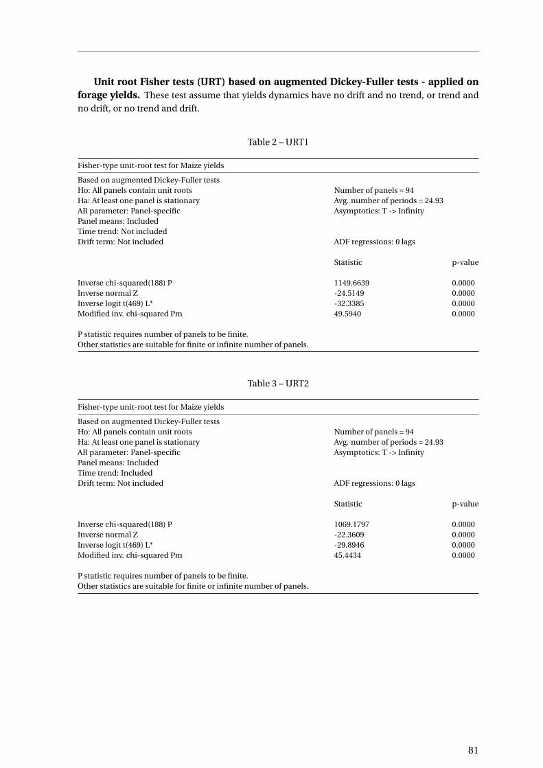
Unit root Fisher tests (URT) based on augmented Dickey-Fuller tests - applied onforage yields. These test assume that yields dynamics have no drift and no trend, or trend and
no drift, or no trend and drift.
Table 2 – URT1
Fisher-type unit-root test for Maize yields
Based on augmented Dickey-Fuller testsHo: All panels contain unit roots Number of panels = 94Ha: At least one panel is stationary Avg. number of periods = 24.93AR parameter: Panel-specific Asymptotics: T -> InfinityPanel means: IncludedTime trend: Not includedDrift term: Not included ADF regressions: 0 lags
Statistic p-value
Inverse chi-squared(188) P 1149.6639 0.0000Inverse normal Z -24.5149 0.0000Inverse logit t(469) L* -32.3385 0.0000Modified inv. chi-squared Pm 49.5940 0.0000
P statistic requires number of panels to be finite.Other statistics are suitable for finite or infinite number of panels.
Table 3 – URT2
Fisher-type unit-root test for Maize yields
Based on augmented Dickey-Fuller testsHo: All panels contain unit roots Number of panels = 94Ha: At least one panel is stationary Avg. number of periods = 24.93AR parameter: Panel-specific Asymptotics: T -> InfinityPanel means: IncludedTime trend: IncludedDrift term: Not included ADF regressions: 0 lags
Statistic p-value
Inverse chi-squared(188) P 1069.1797 0.0000Inverse normal Z -22.3609 0.0000Inverse logit t(469) L* -29.8946 0.0000Modified inv. chi-squared Pm 45.4434 0.0000
P statistic requires number of panels to be finite.Other statistics are suitable for finite or infinite number of panels.
81

Table 4 – URT3
Fisher-type unit-root test for Maize yields
Based on augmented Dickey-Fuller testsHo: All panels contain unit roots Number of panels = 94Ha: At least one panel is stationary Avg. number of periods = 24.93AR parameter: Panel-specific Asymptotics: T -> InfinityPanel means: IncludedTime trend: Not includedDrift term: Included ADF regressions: 0 lags
Statistic p-value
Inverse chi-squared(188) P 1402.11 0.0000Inverse normal Z -30.3047 0.0000Inverse logit t(469) L* -40.0399 0.0000Modified inv. chi-squared Pm 63.0524 0.0000
P statistic requires number of panels to be finite.Other statistics are suitable for finite or infinite number of panels.
Table 5 – URT4
Fisher-type unit-root test for Artificial grassland yields
Based on augmented Dickey-Fuller testsHo: All panels contain unit roots Number of panels = 94Ha: At least one panel is stationary Avg. number of periods = 25.51AR parameter: Panel-specific Asymptotics: T -> InfinityPanel means: IncludedTime trend: Not includedDrift term: Not included ADF regressions: 0 lags
Statistic p-value
Inverse chi-squared(188) P 1314.2409 0.0000Inverse normal Z -27.4870 0.0000Inverse logit t(469) L* -36.9915 0.0000Modified inv. chi-squared Pm 58.0814 0.0000
P statistic requires number of panels to be finite.Other statistics are suitable for finite or infinite number of panels.
82

Table 6 – URT5
Fisher-type unit-root test for Artificial grassland yields
Based on augmented Dickey-Fuller testsHo: All panels contain unit roots Number of panels = 94Ha: At least one panel is stationary Avg. number of periods = 25.51AR parameter: Panel-specific Asymptotics: T -> InfinityPanel means: IncludedTime trend: IncludedDrift term: Not included ADF regressions: 0 lags
Statistic p-value
Inverse chi-squared(188) P 1059.4200 0.0000Inverse normal Z -23.2950 0.0000Inverse logit t(469) L* -29.5221 0.0000Modified inv. chi-squared Pm 44.9401 0.0000
P statistic requires number of panels to be finite.Other statistics are suitable for finite or infinite number of panels.
Table 7 – URT6
Fisher-type unit-root test for Artificial grassland yields
Based on augmented Dickey-Fuller testsHo: All panels contain unit roots Number of panels = 94Ha: At least one panel is stationary Avg. number of periods = 25.51AR parameter: Panel-specific Asymptotics: T -> InfinityPanel means: IncludedTime trend: Not includedDrift term: Included ADF regressions: 0 lags
Statistic p-value
Inverse chi-squared(188) P 1518.3537 0.0000Inverse normal Z -32.1668 0.0000Inverse logit t(469) L* -43.1689 0.0000Modified inv. chi-squared Pm 68.6078 0.0000
P statistic requires number of panels to be finite.Other statistics are suitable for finite or infinite number of panels.
83
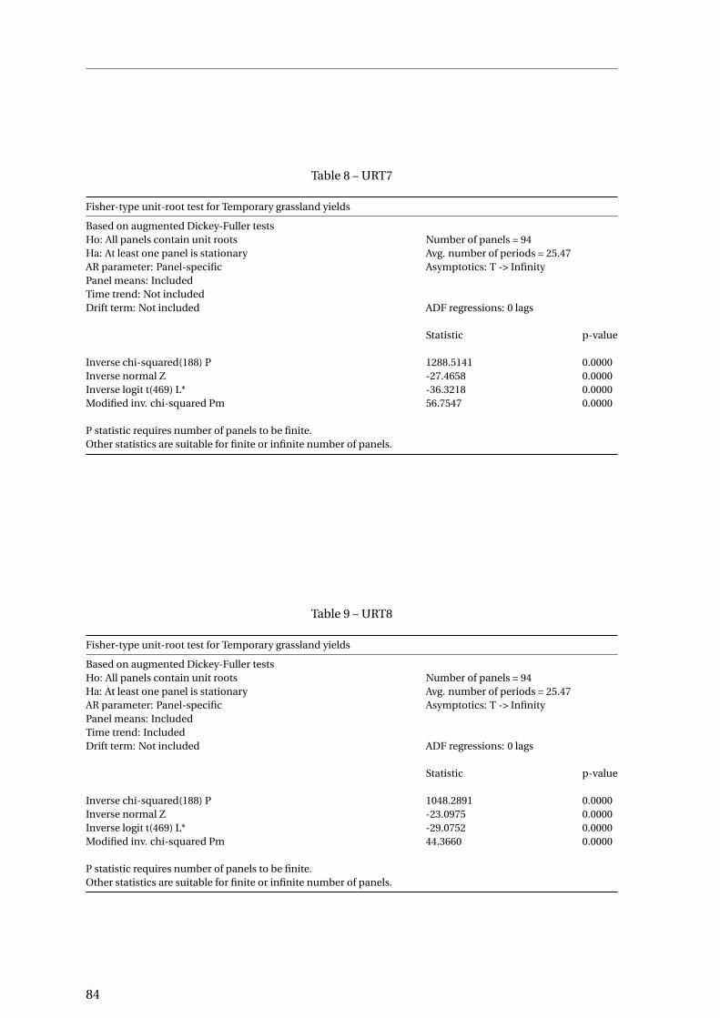
Table 8 – URT7
Fisher-type unit-root test for Temporary grassland yields
Based on augmented Dickey-Fuller testsHo: All panels contain unit roots Number of panels = 94Ha: At least one panel is stationary Avg. number of periods = 25.47AR parameter: Panel-specific Asymptotics: T -> InfinityPanel means: IncludedTime trend: Not includedDrift term: Not included ADF regressions: 0 lags
Statistic p-value
Inverse chi-squared(188) P 1288.5141 0.0000Inverse normal Z -27.4658 0.0000Inverse logit t(469) L* -36.3218 0.0000Modified inv. chi-squared Pm 56.7547 0.0000
P statistic requires number of panels to be finite.Other statistics are suitable for finite or infinite number of panels.
Table 9 – URT8
Fisher-type unit-root test for Temporary grassland yields
Based on augmented Dickey-Fuller testsHo: All panels contain unit roots Number of panels = 94Ha: At least one panel is stationary Avg. number of periods = 25.47AR parameter: Panel-specific Asymptotics: T -> InfinityPanel means: IncludedTime trend: IncludedDrift term: Not included ADF regressions: 0 lags
Statistic p-value
Inverse chi-squared(188) P 1048.2891 0.0000Inverse normal Z -23.0975 0.0000Inverse logit t(469) L* -29.0752 0.0000Modified inv. chi-squared Pm 44.3660 0.0000
P statistic requires number of panels to be finite.Other statistics are suitable for finite or infinite number of panels.
84

Table 10 – URT9
Fisher-type unit-root test for Temporary grassland yields
Based on augmented Dickey-Fuller testsHo: All panels contain unit roots Number of panels = 94Ha: At least one panel is stationary Avg. number of periods = 25.47AR parameter: Panel-specific Asymptotics: T -> InfinityPanel means: IncludedTime trend: Not includedDrift term: Included ADF regressions: 0 lags
Statistic p-value
Inverse chi-squared(188) P 1516.6980 0.0000Inverse normal Z -32.2471 0.0000Inverse logit t(469) L* -43.1281 0.0000Modified inv. chi-squared Pm 68.5224 0.0000
P statistic requires number of panels to be finite.Other statistics are suitable for finite or infinite number of panels.
Table 11 – URT10
Fisher-type unit-root test for Natural and old-seeded grassland yields
Based on augmented Dickey-Fuller testsHo: All panels contain unit roots Number of panels = 95Ha: At least one panel is stationary Avg. number of periods = 25.65AR parameter: Panel-specific Asymptotics: T -> InfinityPanel means: IncludedTime trend: Not includedDrift term: Not included ADF regressions: 0 lags
Statistic p-value
Inverse chi-squared(188) P 1067.7273 0.0000Inverse normal Z -23.1330 0.0000Inverse logit t(469) L* -29.4048 0.0000Modified inv. chi-squared Pm 45.0265 0.0000
P statistic requires number of panels to be finite.Other statistics are suitable for finite or infinite number of panels.
85
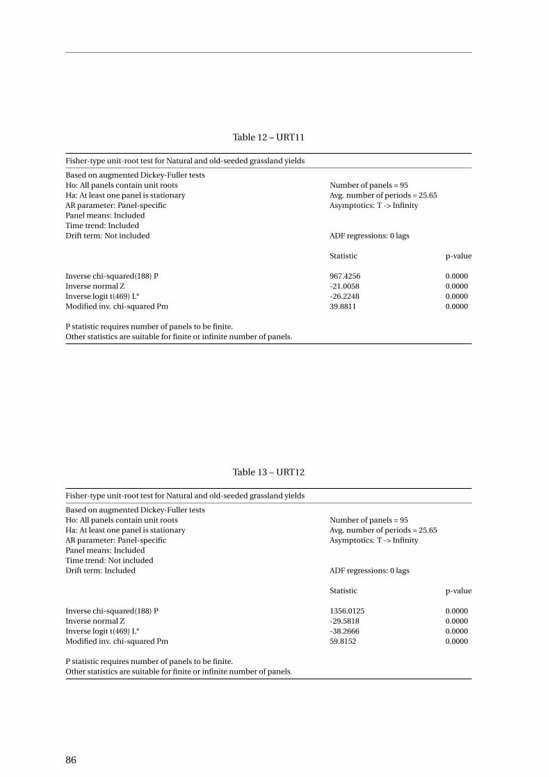
Table 12 – URT11
Fisher-type unit-root test for Natural and old-seeded grassland yields
Based on augmented Dickey-Fuller testsHo: All panels contain unit roots Number of panels = 95Ha: At least one panel is stationary Avg. number of periods = 25.65AR parameter: Panel-specific Asymptotics: T -> InfinityPanel means: IncludedTime trend: IncludedDrift term: Not included ADF regressions: 0 lags
Statistic p-value
Inverse chi-squared(188) P 967.4256 0.0000Inverse normal Z -21.0058 0.0000Inverse logit t(469) L* -26.2248 0.0000Modified inv. chi-squared Pm 39.8811 0.0000
P statistic requires number of panels to be finite.Other statistics are suitable for finite or infinite number of panels.
Table 13 – URT12
Fisher-type unit-root test for Natural and old-seeded grassland yields
Based on augmented Dickey-Fuller testsHo: All panels contain unit roots Number of panels = 95Ha: At least one panel is stationary Avg. number of periods = 25.65AR parameter: Panel-specific Asymptotics: T -> InfinityPanel means: IncludedTime trend: Not includedDrift term: Included ADF regressions: 0 lags
Statistic p-value
Inverse chi-squared(188) P 1356.0125 0.0000Inverse normal Z -29.5818 0.0000Inverse logit t(469) L* -38.2666 0.0000Modified inv. chi-squared Pm 59.8152 0.0000
P statistic requires number of panels to be finite.Other statistics are suitable for finite or infinite number of panels.
86

Table 14 – Control regressions for time effects and multicolinearity
VARIABLES σOUTG σOUW
TG σMATG σMAW
TG σOUAG σOUW
AG σMAAG σMAW
AG σOUNOS σOUW
NOS σMANOS σMAW
NOS
Dummy t1991 -5.555*** 3.163*** -6.881** 3.231*** -2.734*** 1.521***(-2.610) (4.704) (-2.413) (3.904) (-3.025) (3.295)
Dummy t1992 -8.427*** 5.984*** -10.36*** 6.092*** -4.007*** 3.552***(-4.181) (8.827) (-3.873) (6.847) (-4.671) (7.238)
Dummy t1993 -10.00*** 6.510*** -12.58*** 6.698*** -4.868*** 3.941***(-5.119) (9.782) (-4.852) (7.425) (-5.851) (7.971)
Dummy t1994 -11.11*** -0.0574 6.411*** -2.099 -13.70*** 0.596 6.862*** -1.184 -5.435*** -0.505 3.926*** -0.275(-5.751) (-0.0829) (9.679) (-1.607) (-5.396) (0.737) (7.613) (-0.801) (-6.643) (-0.726) (7.948) (-0.282)
Dummy t1995 -12.17*** -0.808 5.839*** -1.996 -14.85*** 0.333 6.328*** -1.551 -5.935*** -1.037 3.570*** -0.296(-6.379) (-1.227) (9.219) (-1.541) (-5.943) (0.448) (7.282) (-1.092) (-7.386) (-1.502) (7.671) (-0.307)
Dummy t1996 -12.49*** -0.673 5.662*** -1.732 -14.96*** 0.733 6.312*** 0.470 -5.902*** -0.387 3.638*** 0.696(-6.576) (-0.920) (9.112) (-1.323) (-6.026) (0.991) (7.450) (0.332) (-7.328) (-0.539) (7.870) (0.663)
Dummy t1997 -13.32*** -0.811 5.292*** -1.987 -15.65*** 0.454 6.192*** -1.328 -6.252*** 0.0673 3.405*** -0.159(-7.054) (-1.142) (8.747) (-1.511) (-6.354) (0.609) (7.547) (-0.894) (-7.836) (0.0959) (7.620) (-0.159)
Dummy t1998 -14.02*** -1.429** 5.064*** -2.135 -16.25*** 0.186 6.162*** -0.761 -6.492*** -0.903 3.334*** -0.731(-7.466) (-2.024) (8.474) (-1.579) (-6.636) (0.257) (7.553) (-0.513) (-8.182) (-1.364) (7.497) (-0.732)
Dummy t1999 -14.10*** -0.473 5.275*** -3.018** -16.37*** 0.910 6.422*** -2.391* -6.544*** -0.696 3.480*** -0.145(-7.509) (-0.647) (8.678) (-2.505) (-6.696) (1.235) (7.800) (-1.793) (-8.255) (-1.026) (7.744) (-0.152)
Dummy t2000 -13.93*** -0.627 5.477*** -0.349 -16.20*** 0.695 6.657*** -0.395 -6.420*** -0.525 3.689*** 0.228(-7.393) (-0.919) (8.824) (-0.254) (-6.631) (0.916) (8.051) (-0.259) (-7.998) (-0.737) (7.880) (0.214)
Dummy t2001 -14.42*** -0.283 5.228*** -1.215 -16.78*** 0.769 6.351*** -0.425 -6.634*** -0.442 3.568*** 0.569(-7.680) (-0.403) (8.528) (-0.839) (-6.893) (1.073) (7.796) (-0.287) (-8.306) (-0.657) (7.709) (0.557)
Dummy t2002 -14.84*** -0.377 5.042*** -1.434 -17.22*** 0.984 6.148*** -0.535 -6.817*** 0.00370 3.482*** 1.249(-7.920) (-0.539) (8.277) (-1.121) (-7.094) (1.385) (7.621) (-0.368) (-8.551) (0.00557) (7.573) (1.145)
Dummy t2003 -13.40*** -0.917 6.192*** 0.560 -15.95*** 0.336 7.222*** 2.042 -6.089*** -0.170 4.337*** 2.185**(-7.161) (-1.309) (10.11) (0.439) (-6.564) (0.452) (8.966) (1.463) (-7.657) (-0.228) (9.355) (2.326)
Dummy t2004 -13.70*** -0.713 6.184*** -2.139 -16.34*** 1.202 7.070*** -0.141 -6.165*** 0.0205 4.588*** 1.355(-7.344) (-0.948) (10.35) (-1.608) (-6.751) (1.556) (8.927) (-0.0999) (-7.764) (0.0292) (10.16) (1.362)
Dummy t2005 -13.88*** -0.881 6.112*** -0.803 -16.63*** 0.343 6.920*** 0.447 -6.249*** -0.735 4.632*** -0.639(-7.450) (-1.259) (10.27) (-0.622) (-6.880) (0.457) (8.805) (0.316) (-7.869) (-1.025) (10.26) (-0.621)
Dummy t2006 -14.12*** -0.216 6.024*** -1.099 -16.93*** 0.600 6.773*** 1.152 -6.352*** -0.143 4.648*** 1.859*(-7.590) (-0.312) (10.22) (-0.813) (-7.015) (0.792) (8.693) (0.727) (-8.003) (-0.195) (10.36) (1.878)
Dummy t2007 -13.92*** -0.373 6.315*** -0.0772 -16.97*** 0.826 6.871*** 1.837 -6.213*** 0.477 5.013*** 2.197**(-7.472) (-0.542) (10.59) (-0.0595) (-7.038) (1.102) (8.828) (1.203) (-7.829) (0.653) (11.30) (2.189)
Dummy t2008 -13.90*** -0.464 6.399*** -0.258 -16.99*** 0.696 6.941*** 1.375 -6.125*** 0.0431 5.225*** 0.956(-7.437) (-0.682) (10.55) (-0.202) (-7.046) (0.950) (8.877) (0.924) (-7.694) (0.0647) (11.68) (0.891)
Dummy t2009 -14.14*** -0.339 6.282*** -1.530 -17.31*** 0.0171 6.751*** -2.289 -6.236*** 0.301 5.180*** 1.304(-7.572) (-0.465) (10.37) (-1.094) (-7.188) (0.0236) (8.660) (-1.548) (-7.844) (0.408) (11.63) (1.265)
Dummy t2010 -14.27*** -0.923 6.228*** -1.591 -17.31*** 0.471 6.784*** 1.200 -6.292*** 0.0195 5.168*** 1.634(-7.646) (-1.380) (10.29) (-1.149) (-7.173) (0.581) (8.615) (0.793) (-7.913) (0.0266) (11.63) (1.547)
Dummy t2011 -14.13*** -0.735 6.363*** -0.448 -17.14*** 0.717 6.949*** 0.356 -6.245*** -0.548 5.236*** 1.599(-7.556) (-1.018) (10.44) (-0.351) (-7.097) (0.935) (8.804) (0.236) (-7.838) (-0.867) (11.73) (1.588)
Dummy t2012 -14.25*** -0.994 6.325*** -1.574 -17.24*** 0.518 6.926*** 1.202 -6.294*** 0.178 5.220*** 0.232(-7.634) (-1.396) (10.45) (-1.180) (-7.147) (0.654) (8.803) (0.810) (-7.909) (0.238) (11.71) (0.219)
Dummy t2013 -14.32*** -0.695 6.310*** 0.256 -17.34*** 0.188 6.899*** -0.471 -6.263*** -0.129 5.284*** 2.257**(-7.698) (-1.002) (10.56) (0.196) (-7.213) (0.264) (8.910) (-0.337) (-7.864) (-0.175) (11.85) (2.178)
Dummy t2014 -14.15*** -0.415 6.470*** 0.186 -17.06*** 0.614 7.161*** 0.438 -6.054*** -0.0391 5.522*** 0.895(-7.603) (-0.595) (10.78) (0.146) (-7.096) (0.828) (9.224) (0.290) (-7.551) (-0.0524) (12.28) (0.874)
Dummy t2015 -14.17*** -0.453 6.492*** -1.699 -17.09*** 0.684 7.177*** -1.381 -6.023*** 0.316 5.559*** -0.624(-7.605) (-0.634) (10.75) (-1.302) (-7.102) (0.907) (9.187) (-0.925) (-7.451) (0.426) (12.15) (-0.599)
Dummy t2016 -14.14*** -0.341 6.537*** -0.690 -17.22*** 0.568 7.106*** 0.932 -6.008*** -0.00680 5.576*** 1.075(-7.591) (-0.515) (10.82) (-0.526) (-7.171) (0.735) (9.187) (0.619) (-7.408) (-0.00978) (12.14) (1.107)
Constant 31.68*** 8.745*** 4.959*** 17.97*** 36.05*** 8.724*** 5.760*** 18.55*** 15.83*** 7.982*** 3.525*** 12.29***(17.90) (17.43) (10.79) (18.95) (15.64) (16.91) (9.321) (18.22) (21.52) (16.98) (10.77) (17.01)
Fixed effects Yes Yes Yes Yes Yes Yes Yes Yes Yes Yes Yes Yes
Observations 2,565 2,074 2,565 2,018 2,565 2,078 2,565 2,022 2,565 2,111 2,565 2,057R-squared 0.166 0.005 0.098 0.012 0.141 0.003 0.073 0.015 0.141 0.006 0.139 0.020F 7.200 0.454 8.850 1.197 5.387 0.315 6.250 1.456 6.247 0.593 15.79 1.917p Fisher 0 0.988 0 0.236 0 0.999 0 0.0746 0 0.936 0 0.00549
Robust t-statistics in parentheses*** p<0.01, ** p<0.05, * p<0.1
87

Table 15 – Yields shocks’ impact on Temporary grasslands ratio
VARIABLES P(TG) P(TG) P(TG) P(TG) P(TG) P(TG)
Negative shocks TG -0.0281(-0.848)
Positive shocks TG 0.0469(1.623)
lag(1) Negative shocks TG 0.0356(1.182)
lag(1) Positive shocks TG 0.0544**(1.994)
Negative shocks AG -0.0217(-0.535)
Positive shocks AG 0.0351(1.047)
lag(1) Negative shocks AG -0.00275(-0.0753)
lag(1) Positive shocks AG 0.0134(0.371)
Negative shocks NOS 0.209(0.736)
Positive shocks NOS 0.839***(2.828)
lag(1) Negative shocks NOS 0.437(1.477)
lag(1) Positive shocks NOS -0.130(-0.626)
Constant 1.037*** 1.032*** 1.039*** 1.061*** 0.835*** 0.632**(53.49) (56.78) (43.66) (43.91) (2.971) (2.156)
Observations 2,314 2,221 2,314 2,221 2,314 2,221R-squared 0.005 0.002 0.003 0.000 0.005 0.004Number of geo 94 94 94 94 94 94F 3.192 1.996 1.632 0.189 12.47p Fisher 0.0456 0.142 0.201 0.828 1.60e-05Robust t-statistics in parentheses*** p<0.01, ** p<0.05, * p<0.1
88

Table 16 – Yields shocks’ impact on Artificial grasslands ratio
VARIABLES P(AG) P(AG) P(AG) P(AG) P(AG) P(AG)
Negative shocks AG 0.00322(0.0834)
Positive shocks AG 0.00475(0.150)
lag(1) Negative shocks AG 0.0309(0.765)
lag(1) Positive shocks AG -0.0185(-0.514)
Negative shocks TG -0.0444(-1.252)
Positive shocks TG -0.0409(-1.110)
lag(1) Negative shocks TG 0.0352(1.220)
lag(1) Positive shocks TG -0.0284(-0.674)
Negative shocks NOS 0.321***(6.006)
Positive shocks NOS 0.921***(4.405)
lag(1) Negative shocks NOS 0.477***(17.60)
lag(1) Positive shocks NOS 0.271***(14.30)
Constant -0.786*** -0.806*** -0.753*** -0.804*** -1.103*** -1.274***(-37.16) (-33.33) (-33.78) (-35.14) (-20.76) (-47.42)
Observations 2,317 2,224 2,316 2,224 2,316 2,224R-squared 0.000 0.001 0.001 0.002 0.004 0.003Number of geo 94 94 94 94 94 94F 0.0115 0.904 0.964 2.155 18.64p 0.989 0.408 0.385 0.122 1.56e-07Robust t-statistics in parentheses*** p<0.01, ** p<0.05, * p<0.1
89

Table 17 – Yields shocks’ impact on Natural and old-seeded grasslands ratio
VARIABLES P(NOS) P(NOS) P(NOS) P(NOS) P(NOS) P(NOS)
Negative shocks NOS -0.0153(-0.113)
Positive shocks NOS 1.189***(3.114)
lag(1) Negative shocks NOS 0.464(1.650)
lag(1) Positive shocks NOS 1.326***(6.743)
Negative shocks TG -0.0459*(-1.720)
Positive shocks TG 0.0278(1.272)
lag(1) Negative shocks TG 0.0254(1.068)
lag(1) Positive shocks TG 0.0379(1.268)
Negative shocks AG -0.0175(-0.499)
Positive shocks AG 0.0425(1.543)
lag(1) Negative shocks AG 0.000478(0.0136)
lag(1) Positive shocks AG 0.0202(0.657)
Constant 2.432*** 1.957*** 2.425*** 2.395*** 2.410*** 2.410***(18.08) (7.025) (168.5) (136.3) (123.2) (115.3)
Observations 2,316 2,223 2,316 2,223 2,316 2,223R-squared 0.017 0.014 0.008 0.002 0.006 0.001Number of geo 94 94 94 94 94 94F 28.03 3.483 0.861 2.326 0.308p Fisher 2.97e-10 0.0348 0.426 0.103 0.735
Robust t-statistics in parentheses*** p<0.01, ** p<0.05, * p<0.1
90

Table 18 – All yields shocks’ impact on the three types of grasslands
VARIABLES P(AG) P(TG) P(NOS) P(AG) P(TG) P(NOS)
lag(1) Negative shocks maize 0.115*** -0.0285 0.0305(0.0366) (0.0399) (0.0282)
lag(1) Positive shocks maize -0.105*** 0.0228 -0.0233(0.0358) (0.0301) (0.0196)
lag(1) Negative shocks TG -0.0107 0.0348 0.0166(0.0420) (0.0304) (0.0249)
lag(1) Positive shocks TG -0.00124 0.0512 0.0368(0.0510) (0.0330) (0.0291)
lag(1) Negative shocks NOS 0.209 0.162 0.291(0.129) (0.139) (0.190)
lag(1) Positive shocks NOS 0.442*** 0.0406 1.439***(0.0844) (0.0887) (0.117)
lag(1) Negative shocks AG 0.00256 0.00174 -0.00726(0.0491) (0.0405) (0.0363)
lag(1) Positive shocks AG 0.00866 -0.00897 0.0119(0.0476) (0.0429) (0.0342)
Negative shocks maize 0.0945** -0.0413 -0.00388(0.0428) (0.0379) (0.0269)
Positive shocks maize -0.107*** 0.0385 -0.0108(0.0338) (0.0295) (0.0193)
Negative shocks TG -0.0854* -0.0248 -0.0549**(0.0480) (0.0362) (0.0227)
Positive shocks TG -0.0225 0.0350 0.0163(0.0459) (0.0335) (0.0265)
Negative shocks NOS 0.274*** 0.259 0.0111(0.0705) (0.278) (0.136)
Positive shocks NOS 0.899*** 0.842*** 1.180***(0.225) (0.312) (0.399)
Negative shocks AG 0.0180 0.0149 0.0191(0.0484) (0.0474) (0.0373)
Positive shocks AG 0.0261 0.00120 0.0220(0.0411) (0.0398) (0.0315)
Constant -1.029*** 0.863*** 2.090*** -1.026*** 0.776*** 2.411***(0.128) (0.141) (0.195) (0.0787) (0.270) (0.132)
Observations 2,218 2,215 2,217 2,316 2,314 2,316R-squared 0.031 0.005 0.021 0.028 0.015 0.026Number of geo 94 94 94 94 94 94F - - - 5.665 4.732 9.091p Fisher - - - 7.34e-06 6.84e-05 3.75e-09
Robust standard errors in parentheses*** p<0.01, ** p<0.05, * p<0.1
91
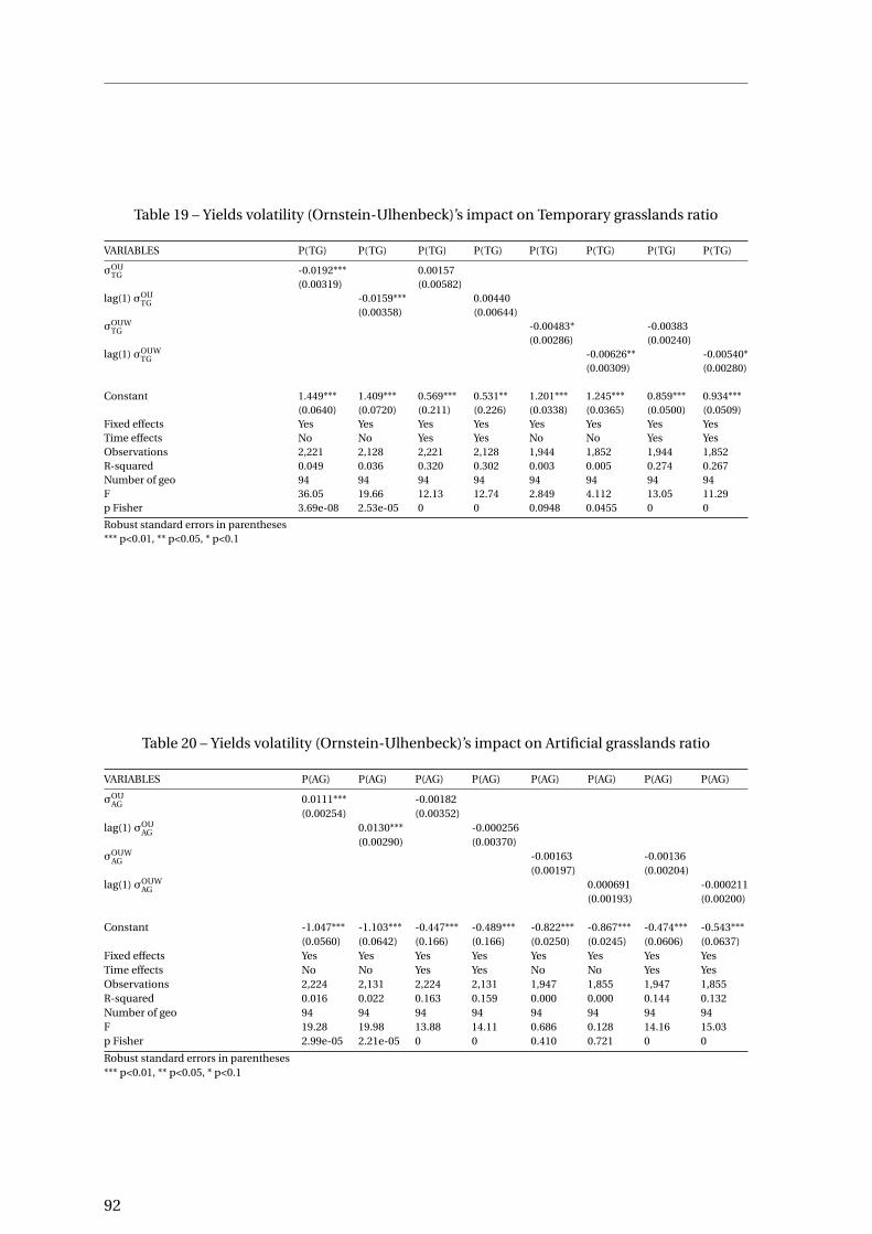
Table 19 – Yields volatility (Ornstein-Ulhenbeck)’s impact on Temporary grasslands ratio
VARIABLES P(TG) P(TG) P(TG) P(TG) P(TG) P(TG) P(TG) P(TG)
σOUTG -0.0192*** 0.00157
(0.00319) (0.00582)lag(1) σOU
TG -0.0159*** 0.00440(0.00358) (0.00644)
σOUWTG -0.00483* -0.00383
(0.00286) (0.00240)lag(1) σOUW
TG -0.00626** -0.00540*(0.00309) (0.00280)
Constant 1.449*** 1.409*** 0.569*** 0.531** 1.201*** 1.245*** 0.859*** 0.934***(0.0640) (0.0720) (0.211) (0.226) (0.0338) (0.0365) (0.0500) (0.0509)
Fixed effects Yes Yes Yes Yes Yes Yes Yes YesTime effects No No Yes Yes No No Yes YesObservations 2,221 2,128 2,221 2,128 1,944 1,852 1,944 1,852R-squared 0.049 0.036 0.320 0.302 0.003 0.005 0.274 0.267Number of geo 94 94 94 94 94 94 94 94F 36.05 19.66 12.13 12.74 2.849 4.112 13.05 11.29p Fisher 3.69e-08 2.53e-05 0 0 0.0948 0.0455 0 0
Robust standard errors in parentheses*** p<0.01, ** p<0.05, * p<0.1
Table 20 – Yields volatility (Ornstein-Ulhenbeck)’s impact on Artificial grasslands ratio
VARIABLES P(AG) P(AG) P(AG) P(AG) P(AG) P(AG) P(AG) P(AG)
σOUAG 0.0111*** -0.00182
(0.00254) (0.00352)lag(1) σOU
AG 0.0130*** -0.000256(0.00290) (0.00370)
σOUWAG -0.00163 -0.00136
(0.00197) (0.00204)lag(1) σOUW
AG 0.000691 -0.000211(0.00193) (0.00200)
Constant -1.047*** -1.103*** -0.447*** -0.489*** -0.822*** -0.867*** -0.474*** -0.543***(0.0560) (0.0642) (0.166) (0.166) (0.0250) (0.0245) (0.0606) (0.0637)
Fixed effects Yes Yes Yes Yes Yes Yes Yes YesTime effects No No Yes Yes No No Yes YesObservations 2,224 2,131 2,224 2,131 1,947 1,855 1,947 1,855R-squared 0.016 0.022 0.163 0.159 0.000 0.000 0.144 0.132Number of geo 94 94 94 94 94 94 94 94F 19.28 19.98 13.88 14.11 0.686 0.128 14.16 15.03p Fisher 2.99e-05 2.21e-05 0 0 0.410 0.721 0 0
Robust standard errors in parentheses*** p<0.01, ** p<0.05, * p<0.1
92

Table 21 – Yields volatility (Ornstein-Ulhenbeck)’s impact on Natural and old-seeded grasslandsratio
VARIABLES P(NOS) P(NOS) P(NOS) P(NOS) P(NOS) P(NOS) P(NOS) P(NOS)
σOUNOS -0.00795 -0.00611
(0.00481) (0.00703)lag(1) σOU
NOS -0.00134 0.000510(0.00496) (0.00678)
σOUWNOS 0.00366 0.00340
(0.00225) (0.00209)lag(1) σOUW
NOS 0.00157 0.00152(0.00229) (0.00226)
Constant 2.500*** 2.434*** 2.442*** 2.363*** 2.399*** 2.417*** 2.388*** 2.398***(0.0497) (0.0513) (0.131) (0.125) (0.0166) (0.0169) (0.0454) (0.0456)
Fixed effects Yes Yes Yes Yes Yes Yes Yes YesTime effects No No Yes Yes No No Yes YesObservations 2,223 2,130 2,223 2,130 1,946 1,854 1,946 1,854R-squared 0.003 0.000 0.043 0.042 0.001 0.000 0.045 0.047Number of geo 94 94 94 94 94 94 94 94F 2.735 0.0734 9.075 9.124 2.642 0.470 9.668 8.708p Fisher 0.102 0.787 0 0 0.107 0.495 0 0
Robust standard errors in parentheses*** p<0.01, ** p<0.05, * p<0.1
Table 22 – Yields volatility (Moving average)’s impact on Temporary grasslands ratio
VARIABLES P(TG) P(TG) P(TG) P(TG) P(TG) P(TG) P(TG) P(TG)
σMATG 0.0451*** 0.00889
(0.00702) (0.00739)lag(1) σMA
TG 0.0434*** 0.00925(0.00693) (0.00788)
σMAWTG -0.00100 -0.00202
(0.00145) (0.00136)lag(1) σMAW
TG 0.000552 -0.000841(0.00126) (0.00116)
Constant 0.565*** 0.610*** 0.575*** 0.628*** 1.161*** 1.161*** 0.849*** 0.885***(0.0779) (0.0765) (0.0619) (0.0602) (0.0249) (0.0217) (0.0409) (0.0444)
Fixed effects Yes Yes Yes Yes Yes Yes Yes YesTime effects No No Yes Yes No No Yes YesObservations 2,221 2,128 2,221 2,128 1,944 1,852 1,944 1,852R-squared 0.071 0.070 0.321 0.303 0.000 0.000 0.273 0.264Number of geo 94 94 94 94 94 94 94 94F 41.26 39.27 13.31 13.61 0.475 0.193 13.61 13.70p Fisher 5.59e-09 1.14e-08 0 0 0.492 0.662 0 0
Robust standard errors in parentheses*** p<0.01, ** p<0.05, * p<0.1
93

Table 23 – Yields volatility (Moving average)’s impact on Artificial grasslands ratio
VARIABLES P(AG) P(AG) P(AG) P(AG) P(AG) P(AG) P(AG) P(AG)
σMAAG -0.0178* 0.00765
(0.00987) (0.0111)lag(1) σMA
AG -0.0165* 0.00859(0.00937) (0.0104)
σMAWAG -0.000402 -0.000493
(0.00175) (0.00150)lag(1) σMAW
AG -0.000326 -0.000445(0.00179) (0.00160)
Constant -0.577*** -0.608*** -0.560*** -0.549*** -0.835*** -0.852*** -0.482*** -0.537***(0.125) (0.118) (0.0959) (0.0896) (0.0337) (0.0346) (0.0626) (0.0605)
Fixed effects Yes Yes Yes Yes Yes Yes Yes YesTime effects No No Yes Yes No No Yes YesObservations 2,224 2,131 2,224 2,131 1,947 1,855 1,947 1,855R-squared 0.009 0.008 0.163 0.160 0.000 0.000 0.144 0.132Number of geo 94 94 94 94 94 94 94 94F 3.241 3.092 14.00 14.43 0.0530 0.0330 15.58 15.65p Fisher 0.0751 0.0820 0 0 0.818 0.856 0 0
Robust standard errors in parentheses*** p<0.01, ** p<0.05, * p<0.1
Table 24 – Yields volatility (Moving average)’s impact on Natural and old-seeded grasslands ratio
VARIABLES P(NOS) P(NOS) P(NOS) P(NOS) P(NOS) P(NOS) P(NOS) P(NOS)
σMANOS 0.00827 -0.00518
(0.00593) (0.00869)lag(1) σMA
NOS 0.00740 -0.00338(0.00581) (0.00903)
σMAWNOS 0.00186 0.00181
(0.00138) (0.00143)lag(1) σMAW
NOS -0.000649 -0.00104(0.00109) (0.000953)
Constant 2.353*** 2.363*** 2.363*** 2.382*** 2.402*** 2.436*** 2.392*** 2.422***(0.0467) (0.0454) (0.0415) (0.0354) (0.0172) (0.0137) (0.0453) (0.0466)
Fixed effects Yes Yes Yes Yes Yes Yes Yes YesTime effects No No Yes Yes No No Yes YesObservations 2,223 2,130 2,223 2,130 1,946 1,854 1,946 1,854R-squared 0.003 0.002 0.043 0.043 0.001 0.000 0.045 0.047Number of geo 94 94 94 94 94 94 94 94F 1.946 1.621 8.861 9.181 1.826 0.354 8.395 8.877p Fisher 0.166 0.206 0 0 0.180 0.553 0 0
Robust standard errors in parentheses*** p<0.01, ** p<0.05, * p<0.1
94

Table 25 – Yields volatility (Ornstein-Uhlenbeck)’s impact with controls on all grasslands ratio
VARIABLES P(TG) P(TG) P(AG) P(AG) P(NOS) P(NOS)
σOUTG -0.0251***
(-4.642)σOUW
TG -0.00333(-0.926)
σOUAG 0.0147***
(2.948)σOUW
AG -0.00234(-0.710)
σOUNOS -0.00829
(-1.176)σOUW
NOS -0.00226(-0.804)
Selling price index for forages -0.00112*** -0.00189*** -0.00196*** -0.00184*** -0.00141*** -0.00179***(-4.742) (-6.498) (-5.353) (-5.371) (-5.003) (-6.561)
Spatialized index for animal costs 0.283** 0.220** 0.101 0.0789 0.201*** 0.167***(2.144) (2.089) (0.507) (0.393) (2.678) (2.749)
Constant 1.370*** 1.131*** -0.940*** -0.611*** 2.461*** 2.495***(8.163) (9.592) (-4.676) (-2.661) (28.92) (32.85)
Fixed effects Yes Yes Yes Yes Yes YesObservations 1,107 985 1,107 985 1,107 985R-squared 0.061 0.024 0.055 0.019 0.022 0.030Number of geo 62 62 62 62 62 62F 19.96 21.19 13.77 10.92 15.25 17.02p Fisher 3.92e-09 1.60e-09 5.77e-07 7.78e-06 1.63e-07 3.83e-08
Robust t-statistics in parentheses*** p<0.01, ** p<0.05, * p<0.1
Table 26 – Yields volatility (Moving average)’s impact with controls on all grasslands ratio
VARIABLES P(TG) P(TG) P(AG) P(AG) P(NOS) P(NOS)
σMATG 0.0353***
(3.123)σMAW
TG -0.00142(-1.000)
σMAAG -0.0150*
(-1.720)σMAW
AG -0.00103(-0.689)
σMANOS 0.00728
(1.278)σMAW
NOS 0.000478(0.398)
Selling price index for forages -0.00133*** -0.00189*** -0.00194*** -0.00183*** -0.00144*** -0.00179***(-5.048) (-6.726) (-4.990) (-5.427) (-5.323) (-6.540)
Spatialized index for animal costs 0.0767 0.224** 0.167 0.0873 0.168** 0.166***(0.814) (2.147) (0.816) (0.435) (2.615) (2.742)
Constant 0.743*** 1.124*** -0.512** -0.623** 2.364*** 2.473***(4.800) (9.598) (-2.021) (-2.652) (24.10) (32.54)
Observations 1,107 985 1,107 985 1,107 985R-squared 0.045 0.024 0.032 0.019 0.022 0.029Number of geo 62 62 62 62 62 62F 9.662 18.06 11.56 11.28 16.39 16.70p Fisher 2.62e-05 1.68e-08 4.27e-06 5.55e-06 6.35e-08 4.92e-08
Robust t-statistics in parentheses*** p<0.01, ** p<0.05, * p<0.1
95

Table 27 – Correlation coefficients table for volatility measures (Ornstein-Uhlenbeck) and meteo-rological data
σOUTG σOUW
TG σOUAG σOUW
AG σOUNOS σOUW
NOS
Average temperature 0.0832* 0.1258* 0.0124 -0.0696* 0.1925* 0.2665*Average effective rainfall -0.1226* -0.1078* -0.0857* -0.0503* -0.1518* -0.1545*Average liquid precipitation -0.1605* -0.0653* -0.1343* -0.0634* -0.1574* -0.1164*Average minimum temperature 0.2270* 0.0014 0.1590* -0.0419* 0.1938* 0.0283Average maximum temperature -0.1830* 0.0905* -0.1475* 0.0059 -0.0955* 0.1577*Average real evapotranspiration 0.0084 -0.1124* 0.0081 -0.0800* -0.0732* -0.1663*Average potential evapotranspiration -0.1904* 0.0736* -0.1563* -0.0382* -0.1048* 0.1846*Average atmospheric radius 0.2508* -0.0431* 0.2292* -0.0241 0.1948* -0.0717*Average visible radius -0.0985* -0.0277 -0.0338 -0.0749* -0.0810* 0.0151Average specific humidity 0.1624* 0.0981* 0.0601* -0.0605* 0.1915* 0.1654*Average relative humidity 0.1866* -0.0361 0.0813* -0.0061 0.0880* -0.1324*Std dev temperature -0.2234* -0.1118* -0.1646* -0.0674* -0.2566* -0.1295*Std dev effective rainfall -0.2156* -0.1722* -0.1283* -0.0687* -0.2311* -0.1462*Std dev liquid precipitation -0.1407* -0.1184* -0.0499* -0.0401* -0.1761* -0.1314*Std dev minimum temperature -0.2449* -0.0349 -0.1909* -0.0533* -0.2536* -0.0823*Std dev maximum temperature -0.2327* -0.0989* -0.1642* -0.0073 -0.2415* -0.1478*Std dev real evapotranspiration -0.2154* -0.0643* -0.1921* -0.0717* -0.2053* -0.0488*Std dev potential evapotranspiration 0.0972* -0.0159 0.0845* -0.0467* 0.0470* -0.0785*Std dev atmospheric radius 0.2470* -0.0417* 0.2239* -0.0322 0.1911* -0.0741*Std dev visible radius -0.0120 -0.1242* 0.0480* 0.0226 -0.1188* -0.1885*Std dev specific humidity -0.1397* -0.1119* -0.1336* -0.0755* -0.1772* -0.0769*Std dev relative humidity 0.1104* -0.0716* 0.1267* -0.0222 0.0215 -0.1228*
Table 28 – Correlation coefficients table for volatility measures (Moving average) and meteorolog-ical data
σMATG σMAW
TG σMAAG σMAW
AG σMANOS σMAW
NOS
Average temperature 0.0754* 0.0745* 0.0222 0.0913* 0.0916* 0.1183*Average effective rainfall -0.1219* -0.1338* -0.0985* -0.2007* -0.0992* -0.1651*Average liquid precipitation -0.0174 -0.0893* -0.0151 -0.1095* 0.0328 -0.1093*Average minimum temperature -0.0659* -0.0155 -0.0989* -0.0038 -0.1678* -0.0432*Average maximum temperature 0.1112* 0.0881* 0.1331* 0.1188* 0.2130* 0.1403*Average real evapotranspiration -0.0029 -0.1257* -0.0047 -0.0953* -0.0057 -0.1454*Average potential evapotranspiration -0.0705* -0.0852* -0.0380* -0.0292 0.0048 -0.0413*Average atmospheric radius -0.1329* -0.0710* -0.1199* -0.0697* -0.2474* -0.0939*Average visible radius -0.0986* -0.2159* -0.0423* -0.1538* -0.0608* -0.1970*Average specific humidity 0.1443* 0.1494* 0.0673* 0.1172* 0.1203* 0.1358*Average relative humidity 0.2497* 0.1923* 0.1643* 0.1335* 0.1898* 0.1332*Std dev temperature -0.2294* -0.2827* -0.1848* -0.2692* -0.2141* -0.3243*Std dev effective rainfall -0.2114* -0.2284* -0.1465* -0.2657* -0.1824* -0.3027*Std dev liquid precipitation -0.1995* -0.1830* -0.1441* -0.2048* -0.2194* -0.2652*Std dev minimum temperature -0.1451* -0.1855* -0.1162* -0.1983* -0.1091* -0.2230*Std dev maximum temperature -0.1994* -0.1919* -0.1625* -0.1858* -0.1757* -0.2602*Std dev real evapotranspiration -0.2090* -0.2034* -0.1975* -0.1896* -0.1811* -0.2920*Std dev potential evapotranspiration -0.2089* -0.1438* -0.1858* -0.1361* -0.2895* -0.1979*Std dev atmospheric radius -0.1310* -0.0724* -0.1205* -0.0782* -0.2456* -0.1010*Std dev visible radius -0.0081 -0.0329 0.0483* -0.0247 -0.0246 -0.1772*Std dev specific humidity -0.1479* -0.2079* -0.1508* -0.2350* -0.1561* -0.2679*Std dev relative humidity -0.1275* -0.1243* -0.0974* -0.1001* -0.2607* -0.1869*
96

Table 29 – Instrumentation of yields volatility (Ornstein Uhlenbeck)’s impact on all grasslands ra-tios
VARIABLES P(TG) P(TG) P(AG) P(AG) P(NOS) P(NOS)
σOUTG -0.120***
(0.00989)σOUW
TG -0.170***(0.0581)
σOUAG 0.0761***
(0.00768)σOUW
AG -0.779(1.050)
σOUNOS 0.396***
(0.152)σOUW
NOS -4.291(57.75)
Observations 2,167 1,274 2,170 1,274 1,274 1,274R-squared -1.356 -2.457 -0.532 -23.162 -1.349 -1,650.212Number of geo 92 77 92 77 77 77F 146.5 8.592 98.20 0.549 6.821 0.00552P Fisher 0.0000 0.0034 0.0000 0.4587 0.0091 0.9408
Robust standard errors in parentheses*** p<0.01, ** p<0.05, * p<0.1
Overidentification testHansen J stat - Chi2 p value 0.8025 - - - 0.9835 -Underidentification testLM test - Chi2 p value 0.0000 0.0004 0.0000 0.4481 0.0022 0.9409Endogeneity postestimation testSargan Hansen test - Chi2 p value 0.0000 0.0000 0.0000 0.0036 0.0010 0.0013
Validation in terms of instrumentation Yes Yes Yes No Yes NoValidation in global inference (Fisher) Yes Yes Yes No Yes No
97

Table 30 – Instrumentation of yields volatility (Moving average)’s impact on all grasslands ratios
VARIABLES P(TG) P(TG) P(AG) P(AG) P(NOS) P(NOS)
σMATG 0.0602**
(0.0267)σMAW
TG -0.854(4.646)
σMAAG -0.155***
(0.0187)σMAW
AG -0.483(0.635)
σMANOS 0.0296***
(0.00822)σMAW
NOS -0.140**(0.0615)
Observations 2,167 1,274 2,170 1,899 2,169 1,274R-squared 0.064 -318.104 -0.552 -44.334 -0.015 -5.535Number of geo 92 77 92 92 92 77F 5.091 0.0337 68.72 0.579 12.92 5.199p Fisher 0.0242 0.8543 0.0000 0.4470 0.0003 0.0228
Robust standard errors in parentheses*** p<0.01, ** p<0.05, * p<0.1
Overidentification testHansen J stat - Chi2 p value - - - - - 0.9392Underidentification testLM test - Chi2 p value 0.0000 0.8542 0.0000 0.4397 0.0000 0.0354Endogeneity postestimation testSargan Hansen test - Chi2 p value 0.5672 0.0032 0.0000 0.0000 0.0044 0.0000
Validation in terms of instrumentation No No Yes No Yes YesValidation in global inference (Fisher) Yes No Yes No Yes Yes
98
Chapter 4
Role of farmers’ risk and ambiguitypreferences on fertilization decisions: anexperiment
Contents4.1 Introduction . . . . . . . . . . . . . . . . . . . . . . . . . . . . . . . . . . . . 100
4.2 Literature review . . . . . . . . . . . . . . . . . . . . . . . . . . . . . . . . . 101
4.3 Questionnaire . . . . . . . . . . . . . . . . . . . . . . . . . . . . . . . . . . . 103
4.3.1 Part 1 of the questionnaire: Elicitation of preferences . . . . . . . . . 103
4.3.2 Participants, order effect and incentives . . . . . . . . . . . . . . . . 104
4.3.3 Parts 2 and 3 of the questionnaire: fertilization and socio-demographiccharacteristics . . . . . . . . . . . . . . . . . . . . . . . . . . . . . . . . 105
4.4 Results . . . . . . . . . . . . . . . . . . . . . . . . . . . . . . . . . . . . . . . 106
4.4.1 Elicitation of risk and ambiguity preferences . . . . . . . . . . . . . . 106
4.4.2 Descriptive statistics . . . . . . . . . . . . . . . . . . . . . . . . . . . . 109
4.4.3 Pairwise correlations and marginal impact estimations . . . . . . . 115
4.5 Conclusion . . . . . . . . . . . . . . . . . . . . . . . . . . . . . . . . . . . . . 118
99

CHAPTER 4. ROLE OF FARMERS’ RISK AND AMBIGUITY PREFERENCES ONFERTILIZATION DECISIONS: AN EXPERIMENT
4.1 Introduction
Reducing GHG emissions in the agricultural sector is a major environmental policy chal-lenge in France, where the sector was responsible in 2017 for 20.4% of the total GHG emis-sions (CITEPA [15]). The agricultural sector, associated to the forest one, is the main sectorable to sequester atmospheric carbon, so that it represents a great potential of mitigation.Mitigation practices that are proposed to farmers in the context of the European CommonAgricultural Policy (CAP) encourage farmers to diversify their activities, integrate legumi-nous crop, improve land rotation, develop better link between a good feeding for the live-stock and vegetal protein production, and especially limit the use of pollutant inputs. Inthis context, reducing synthetic nitrogenous fertilization or improving fertilization effi-ciency is an important mitigation strategy.
However, farmers poorly adopt such practices, even when they are associated to neg-ative abatement costs such as the reduction of nitrogenous fertilization (Pellerin et al.[33]). Several determinants of the non-adoption have been identified in the literature.For example, the level of education and the farm size were the most reliable variables thatseem to significantly positively impact adoption. Our idea is that hidden costs linked tothe existence of uncertainty may explain (almost partly) the non-adoption of fertilizationreduction to mitigate climate change. Indeed, adoption of new practices generate pro-duction uncertainty on the farmer’s profits1. The farmers are not certain of the efficiencyof the practices, and the resulting outcome is uncertain. For example, fertilization is arisk-decreasing activity, so that changing the farmer’s habits may be difficult, in partic-ular because the reduction of fertilization is associated to uncertain effect on the profit.As a consequence, the farmer’s preferences toward risk and ambiguity should also play arole in this adoption process. In this context, the question that we address is the following: What is the impact of farmer’s preferences towards risk and ambiguity on fertilizationchoices ? In line with that question, the role of the follow-up advices (in terms of fertiliza-tion) provided by the agent of the agricultural cooperative will also be analyzed.
This research question refers to two different literatures aiming at the elicitation offarmer’s risk and ambiguity preferences. The first literature gathers studies based on re-vealed preferences method, which provides an estimate based on real farmer’s choices(production, input). The second literature is composed with articles using stated pref-erences method. This method provides a quantification of the risk attitude through ex-periment based on simple decisions taken in a controlled environment to provide a puremeasurement. In this paper, we propose to elicit risk and ambiguity aversion parametersthrough simple lottery choices, and then, to use these parameters as potential explana-tory variables for farmer’s fertilization choices. We then combine experimental data onrisk and ambiguity aversion with real data on the fertilization choices and follow-up ad-vices2.
The rest of the paper is organized as follows. In Section 4.2 we precisely position ourresearch as regard to the two literatures briefly evoked above, the one using revealed pref-erences method and the other based on stated preferences method. Section 4.3 presents
1In addition to production uncertainty, a price uncertainty may also appeared. However, as the mitiga-tion practice considered (fertilization) does not imply a change of the agricultural product or a change ofmarket, we only focused on production uncertainty.
2A similar approach has been proposed in Brunette et al. [11] where risk preferences parameter has beenestimated through lottery choices and then used to explain the probability to harvest of foresters.
100
CHAPTER 4. ROLE OF FARMERS’ RISK AND AMBIGUITY PREFERENCES ONFERTILIZATION DECISIONS: AN EXPERIMENT
the questionnaire. The results are presented in Section 4.4, and Section 4.5 provides thediscussion and conclusion of the paper.
4.2 Literature review
Following the modeling approaches of Moschini and Hennessy [32], Pope and Kramer[34], and Roosen and Hennessy [36], inter alia, the use of an input by a producer can beimpacted by risk if the input is risk-increasing or decreasing (in yields), depending on theproducer’s risk preferences: a risk averse agent will use less of a risk increasing input thana risk neutral one, and reciprocally. This result has been specifically extended in the caseof input use and agricultural policies by Leathers and Quiggin [28] who show that a policycan be partly inefficient if the risks associated to the input and producer’s preferences to-ward risk are not taken into account. For instance, taxing a risk-increasing polluting inputin order to disincentive its use by farmers can lead to disappointing results because riskaverse farmers can try to maintain a sufficiently high level of its use to avoid risk. Thisphenomenon can explain why yields risk and risk preferences are hidden costs of pol-lution policies, especially for agricultural policies, and low level of participation can beobserved.
The relationships between nitrogenous fertilization and risk is well-documented inempirical studies, that especially use revealed preferences methods or agronomic simula-tions. Stuart et al. [38] show that applying more nitrogenous fertilizer is a risk-decreasingactivity, and depends on farmers’ perception about risk and their trust in the informa-tion provided about fertilization reduction. Financial insertion and background risks,as well as the level of competition and the dependency toward contractors create risksthat prevent farmers from reducing their use of nitrogenous fertilizer to maintain a suf-ficient level of yields. Sheriff [37] shows that all farmers put a nitrogenous fertilizer rateaccording to the yields expectation independently of risk preferences, thus uncertaintyimpacts this rate. Moreover, risk aversion and risk perception impact fertilizer use byfarmers, in the same way than in the Pope and Kramer [34] rationale: it depends on therisk-decreasing or risk-increasing nature of the input. Bontems and Thomas [8] studythe role of risk aversion and additional information on nitrogenous fertilizers applica-tions, and found that a large proportion of their sample of farmers was risk averse, andrisk aversion led to an over-fertilization accounting for 7.1% of total fertilizer costs perhectare on average. The value of information, associated to the practice of fertilizationsplittings and observation of nitrogen availability between splits, account for 23.53% offertilizer costs per hectare. Dequiedt and Servonnat [17] developed the mathematicalconditions for risk aversion to lead to higher rate of fertilization. They tested their re-sults on a sample and found that an important proportion of French farmers were riskaverse and that these preferences led to 29.4% more nitrogenous applications by hectare.This account for approximately e75.8/ha, and increase the marginal abatement costs offertilization reduction. The gains that farmers can receive if the application recommen-dations by extension agents would take into account risk and risk aversion have beenstudied by Gandorfer et al. [22]. Through different measures of risk, they compute theoptimal level of nitrogenous rate in different scenarii in order to reach certainty equiva-lents in the same perspective than objective yields. Among their results, they found thatfertilization decreases especially the probability of negative profits, and for the scenarii ofhigh risk aversion the consideration of risk premia leads to an average gains per hectarefor the farmers. Monjardino et al. [31] also show that the risk and risk preferences sig-
101

CHAPTER 4. ROLE OF FARMERS’ RISK AND AMBIGUITY PREFERENCES ONFERTILIZATION DECISIONS: AN EXPERIMENT
nificantly modify the level of optimal nitrogenous fertilization to apply in order to closethe gap between certain yields goals and actual yields. Globally, the theoretical resultsof the modeling approaches are often validated by empirical studies, showing that riskperception, risk preferences and arbitrage between yields mean and variance, impact thelevel of nitrogenous fertilization. This relationship depends on natural conditions, but isrelatively robust in one direction: risk aversion seems to incentive farmers to apply morefertilizer rate on their crops, and consequently increases the cost of reducing applications.Other elements related to uncertainty and information, trust in information sources andrisk profile of farmers have also a role to play.
More recently, another literature emerged based on experimental economics and pro-posed to elicit risk and ambiguity aversion parameters through simple lottery choices.Measuring directly risk attitudes through experiments offers diverse advantages. It allowsfor the specific isolation of risk attitudes from other behavioral parameters because of thedesign of the experimentation: contextualized or not, it aims to purely measure the riskattitudes, and not estimating them like with the revealed preferences methods. It thusprevents some endogeneity biases related to the simultaneous contribution of percep-tions, context and individual preferences to the final decision. Binswanger [4] is the firstto submit lotteries to samples of farmers in order to elicit their risk preferences. The ex-periment presents a comparison of lotteries from the less to the riskier, and ask farmersto choose their preferred lotteries. The more they like risky lotteries, the more risk lovingthey are, and reciprocally. The author found that Indians farmers were on average riskaverse, and that it can have an influence on a lot of phenomenon (investment, credit, in-novation adoption etc.). These initial researches served as an impulse in the literature,so that lots of elicitation procedures appeared. One of the famous procedure, the Mul-tiple Price List (MPL) method, was popularized by Holt and Laury [25]. The idea is tosubmit to the subjects ten paired-lottery choices, and to observe the switching point, i.e.the choice for which they switch from the safe option to the risky one. This switchingpoint allows then to infer a coefficient of relative risk aversion, supposing a power utilityfunction3. This MPL method has already been used to elicit the farmer’s risk preferences.Reynaud and Couture [35] implemented an experiment with French farmers aiming tocompare three different elicitation procedures among which the MPL one. They showthat the estimate of risk aversion is procedure-dependent. Bocquého et al. [6] conductedan experiment on a sample of 100 French farmers, and show that they exhibited attitudesin accordance to expected utility preferences assumption, and that they were risk averse.Chakravarty and Roy [14] extended this MPL procedure to ambiguity aversion elicitation.Their respondents were risk averse but ambiguity neutral in the gain domain, but riskseeking and ambiguity seeking in the loss domain. Bougherara et al. [9] elicited the riskand ambiguity preferences of 197 French farmers. They show that farmers are risk andambiguity averse.
The estimates provided by experimental economics are often used to explain real agri-cultural decisions. The studies that did this provided divergent results. Ghadim et al. [23]showed that Australian farmers adopt new crops depending on their risk aversion, riskperceptions and the perceived covariance between the yields of the different crops. Cottyet al. [16] found that impatient farmers tend to secure their current consumption by fer-
3Other procedures follow with for example the Ordered Lottery Selection (OLS) method popularized byEckel and Grossman [19]. In this procedure, the subject has to indicate at which lottery she accepts to playamong five ones.
102

CHAPTER 4. ROLE OF FARMERS’ RISK AND AMBIGUITY PREFERENCES ONFERTILIZATION DECISIONS: AN EXPERIMENT
tilizing more if they are risk averse, while patient farmers do the reverse if they are riskaverse because they need to smooth their consumption over time. Hellerstein et al. [24],through a Holt and Laury’s experiment, found that more risk aversion led to less diversi-fication, less likelihood to adopt an insurance contract. Liu [29] shows that risk aversioncan lead to significant delay in adoption of new varieties of crops. Engle-Warnick et al.[20] and Barham et al. [1] both observed with experiments (respectively in Peru and inthe US) that ambiguity aversion decreases the probability to adopt a new crop variety iffarmers are not sure of the associated distribution of yields or if the new variety increasesthe level of ambiguity about yields. In the latter, the authors even show that risk aversionhas no impact on adoption of risk-decreasing crop, suggesting that ambiguity alone cansometimes has an effect per se.
4.3 Questionnaire
The questionnaire was in three parts (see Appendix 4.5). The first one was composedof lottery choices to elicit risk aversion and ambiguity aversion parameters. The secondpart is related to the farmers’ practices in terms of fertilization and also contains someinformation about their property. The last part is dedicated to socio-demographic char-acteristics.
4.3.1 Part 1 of the questionnaire: Elicitation of preferences
The preferences are elicited through a MPL method, as proposed by Holt and Laury [25]for risk, and Chakravarty and Roy [14] for ambiguity. Appendix 4.5 presents the lotterychoices under risk and ambiguity. For each task, individuals are presented with ten deci-sions between two lotteries (Option A and Option B). For each decision, the subject has tochoose between a safe option (Option A) and a risky one (Option B) for risk (Table 8), andbetween a risky decision (Option A) and an ambiguous one (Option B) for ambiguity (Ta-ble 9). The number of safe choices allows to infer a coefficient for the relative risk aversioncoefficient assuming a power utility function as: U(x) = xr with r the relative risk aversioncoefficient and x the wealth. The expected utility is given by Eu(x) = pU(x) with p theobjective probability associated to a set of risky outcomes. Table 4.1 presents this classi-fication. Under the same assumption, Table 4.2 presents the classification for ambiguityaversion following Chakravarty and Roy [14] for their φ function representing ambiguitypreferences. Given s the subjective probability belief over a set of ambiguous outcomes,the total expected value function over outcomes can be written as V(x) = sφ[Eu(x)], withφ(z) = za . The concavity of U gives the level of risk aversion, while the concavity ofφ givesthe level of ambiguity aversion.
From these tables two indicators may be extracted. The first one is the number ofsafe choices to represent risk aversion and the number of risky choices to represent theambiguity aversion. In both cases, the higher the number is, the higher the strength of theaversion will be. The second indicator that may be computed is an individual’s averagerisk and ambiguity coefficient. Indeed, using the center of the interval, we can attributeto each subject their corresponding coefficient. These two indicators are then used as afarmer’s characteristic and considered as a potential explanatory variable for fertilizationchoices.
103

CHAPTER 4. ROLE OF FARMERS’ RISK AND AMBIGUITY PREFERENCES ONFERTILIZATION DECISIONS: AN EXPERIMENT
Table 4.1 – Risk aversion classification based on lottery choices
Number of Bounds for relative Classificationsafe choices risk aversion
0 and 1 r <−0.95 Highly risk-loving2 −0.95 < r <−0.49 Very risk-loving3 −0.49 < r <−0.15 Risk-loving4 −0.15 < r < 0.15 Risk-neutral5 0.15 < r < 0.41 Slightly risk averse6 0.41 < r < 0.68 Risk averse7 0.68 < r < 0.97 Very risk averse8 0.97 < r < 1.37 Highly risk averse
9 and 10 1.37 < r Stay in bed
Table 4.2 – Ambiguity aversion classification based on lottery choices
Number of Bounds for relative Classificationrisky choices ambiguity aversion
0 s > 1.92 Extremely ambiguity-loving1 1.92 < s < 1.59 Highly ambiguity-loving2 1.59 < s < 1.35 Very ambiguity-loving3 1.35 < s < 1.15 Ambiguity-loving4 1.15 < s < 1 Slightly ambiguity-loving5 1 < s < 0.86 Ambiguity neutral6 0.86 < s < 0.75 Slightly ambiguity averse7 0.75 < s < 0.66 Ambiguity averse8 0.66 < s < 0.43 Very ambiguity averse9 0.43 < s < 0.30 Highly ambiguity averse
10 s ≥ 0.30 Extremely ambiguity averse
4.3.2 Participants, order effect and incentives
The questionnaire was submitted to a sample of 45 French farmers from four French agri-cultural cooperatives. The questionnaire was realized during meetings organized by thecooperatives, between November 2018 and March 2019. The researchers were presentduring the meeting to present the questionnaire and answer to any potential questionsfrom the farmers.
The first part of the questionnaire used methodology from experimental economicsto elicit farmer’s preferences. In this part, we don’t use financial incentives as traditionallydone in such tasks in experimental economics. Several reasons explain this choice. First,this is a common practice to not incentivize the elicitation task when experiment used“real subjects” as farmers (see Reynaud and Couture [35]) or forest owners (Brunette et al.[10]; Brunette et al. [11]). In addition, Camerer and Hogarth [13] and Beattie and Loomes[3] showed that, since questions are related to simple lottery choices, monetary incentivesdo not seem to significantly affect the decisions. In the same vein, some papers show theabsence of difference in terms of decisions between lottery choices using hypothetical orreal payoffs (Battalio et al. [2], Wik et al. [40]).
Another concern when using elicitation task from experimental economics is the or-
104

CHAPTER 4. ROLE OF FARMERS’ RISK AND AMBIGUITY PREFERENCES ONFERTILIZATION DECISIONS: AN EXPERIMENT
der effect, i.e. the order in which the subjects answer to the various tasks. In order tocontrol for order effect, half of the distributed questionnaire begun with the elicitation ofpreferences towards risk first and then, the elicitation of ambiguity preferences, and theopposite occurs for the other half.
4.3.3 Parts 2 and 3 of the questionnaire: fertilization and socio-demographiccharacteristics
The survey specifically focuses on the bigger parcel of the farmer’s exploitation (exceptgrasslands). The bigger parcel is more likely to host the main crop of the exploitation dur-ing the agricultural campaign and the crop for which the farmer expects to grow most ofher profits (scale effect, intensity effect). Specific questions associated to parameters thatcan explain the nitrogenous needs, and the nitrogenous fertilization decisions are askedin order to provide relevant control variables: spreadable area on the parcel, type of prece-dent crop, soil type, potential organic fertilizer use and fertilizer tillage. Parcel locations(department, municipalities) as well as the status of the farmer with this parcel (owner,tenant) and the potential cropping contract are asked too.
The actual and expected yields are crucial for the farmers since the risk the farmerwould face relative to fertilization is related to how she seeks to reach this yields objec-tive. Since actual yields give us vague general information about the level of efficiency offertilization decisions, the yields goal before the end of the campaign is a proxy of whatyields could have be expected at the beginning and the difference between both is a proxyof the actual shocks that farmer faces on the crop. We expect to use this proxy as a poten-tial explanatory variable of the fertilization’s level, in interaction with risk and ambiguitypreferences.
Concerning the synthetic nitrogenous fertilization, precise questions have been asked.The synthetic nitrogenous fertilization and its potential N2O emission depends on multi-ple parameters: the dose of fertilizer, the spreading method type, the splitting of spreadingaccording to the plant needs, all those elements being related to the current regulation onnitrogenous fertilization. We thus explore all these elements in order to have a completeview of how can synthetic nitrogenous be used, and we associated these elements to theregulation, and more important, to the advices farmers received about them from theircooperative agent. To sum-up the fertilization part, as we want to test the way risk andambiguity preferences can impact N2O emission from synthetic nitrogenous fertilizationand the capacity to follow the official advices about fertilization, we seek quantity andquality variables about actual fertilization, and also quantity and quality variables aboutadvices in order to construct difference variables. In order to gather more control vari-ables, we asked farmers the amount they receive from CAP subsidies (and the specificpart associated to “green” behaviors), if they contracted an optional yields insurance, thetotal area of their farm and their possible participation in a farmers union.
In a last part we asked classical questions about socio-demographic variables that canimpact risk and ambiguity preferences as well as global economic behaviors and charac-teristics of the farmers. Age, marital status, education as well as revenues (inter alia) wereasked, and two last questions with free text answer about opinion of the farmer aboutfertilization and fertilization regulation, and about the present survey. The survey is to-tally anonymous, in order to ensure farmers that their response concerning fertilization
105

CHAPTER 4. ROLE OF FARMERS’ RISK AND AMBIGUITY PREFERENCES ONFERTILIZATION DECISIONS: AN EXPERIMENT
(a sensitive topic) will not be associated to them.
4.4 Results
4.4.1 Elicitation of risk and ambiguity preferences
These graphs show the results of risk and ambiguity preferences elicitation for all the sam-ple (35 non empty answers).
Figure 4.1 – Number of safe choices selected by the farmers
Figure 4.2 – Number of risky choices selected by the farmers
106

CHAPTER 4. ROLE OF FARMERS’ RISK AND AMBIGUITY PREFERENCES ONFERTILIZATION DECISIONS: AN EXPERIMENT
Figure 4.3 – Number of risky choices selected by the farmers
Figures 4.1 and 4.2 show the distributions of preferences in our sample. The aver-age Number of Safe Choices (NSC - risk) is 6, while the average Number of Risky Choices(NRC - ambiguity) is around 5. The major part of respondents is risk averse (70.27%) while14.86% of farmers are risk neutral and the remaining 14.86% are risk loving. The majorpart of respondents is ambiguity neutral (38.24%) and ambiguity loving (38.24) and 23.5%are ambiguity averse (34 non empty answers). Each number of safe (risky) choices corre-sponds to a range of coefficients of risk (ambiguity) aversion. We attribute a coefficientto each number of safe (risky) choices by taking the midpoint of each class, so that eachrespondent has a coefficient4. The average coefficient of risk aversion is 0.615 (preva-lence of risk aversion) and the average coefficient of ambiguity aversion is 0.91 (close toambiguity neutrality). These results are in line with the findings of Bougherara et al. [9]for risk aversion (0.614), but not for the ambiguity aversion (0.722), where the French re-spondents farmers were more ambiguity averse. The results are very close from those ofBarham et al. [1], finding a prevalence of risk aversion preferences in terms of populationproportion, and 38% of ambiguity neutrality, 38% of ambiguity loving and 24% of ambi-guity aversion on a sample of Midwestern (US) farmers. The good fit of our measureswith some results from these previous researches is an important outcome, in terms ofreplicability and external validity of the elicitation methodology. The Figure 4.3 presentsbox plots of the dispersion of preferences for risk and ambiguity in our sample. We cansee that the risk lottery’s responses are more spread than for the ambiguity lottery’s re-sponses, but the later present some outliers.
We constructed a categorical variable with three modalities: if the respondent is risk(ambiguity) loving it takes the value 1, if the respondent is risk (ambiguity) neutral it takesthe value 2, if the respondent is risk (ambiguity) averse it takes the value 3. The modality2 is attributed if the farmer made 4 safe choices in the risk experiment and 5 risky choicesin the ambiguity experiment. If the answer is below this neutrality number, the farmer is
4For the extreme categories we assume 2 and -2 under risk (as Reynaud and Couture [35]), which corre-spond to 2.55 and -0.75 under ambiguity if we assume the same computation method.
107
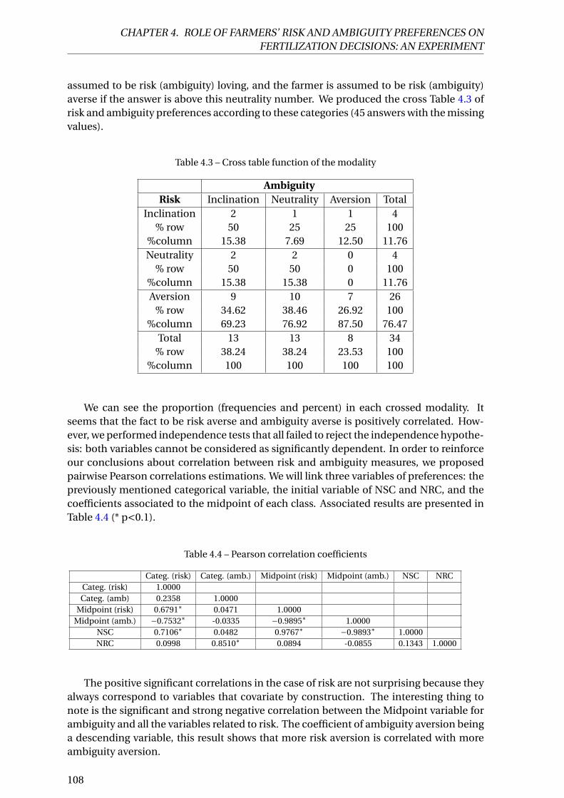
CHAPTER 4. ROLE OF FARMERS’ RISK AND AMBIGUITY PREFERENCES ONFERTILIZATION DECISIONS: AN EXPERIMENT
assumed to be risk (ambiguity) loving, and the farmer is assumed to be risk (ambiguity)averse if the answer is above this neutrality number. We produced the cross Table 4.3 ofrisk and ambiguity preferences according to these categories (45 answers with the missingvalues).
Table 4.3 – Cross table function of the modality
AmbiguityRisk Inclination Neutrality Aversion Total
Inclination 2 1 1 4% row 50 25 25 100
%column 15.38 7.69 12.50 11.76Neutrality 2 2 0 4
% row 50 50 0 100%column 15.38 15.38 0 11.76Aversion 9 10 7 26
% row 34.62 38.46 26.92 100%column 69.23 76.92 87.50 76.47
Total 13 13 8 34% row 38.24 38.24 23.53 100
%column 100 100 100 100
We can see the proportion (frequencies and percent) in each crossed modality. Itseems that the fact to be risk averse and ambiguity averse is positively correlated. How-ever, we performed independence tests that all failed to reject the independence hypothe-sis: both variables cannot be considered as significantly dependent. In order to reinforceour conclusions about correlation between risk and ambiguity measures, we proposedpairwise Pearson correlations estimations. We will link three variables of preferences: thepreviously mentioned categorical variable, the initial variable of NSC and NRC, and thecoefficients associated to the midpoint of each class. Associated results are presented inTable 4.4 (* p<0.1).
Table 4.4 – Pearson correlation coefficients
Categ. (risk) Categ. (amb.) Midpoint (risk) Midpoint (amb.) NSC NRCCateg. (risk) 1.0000Categ. (amb) 0.2358 1.0000
Midpoint (risk) 0.6791∗ 0.0471 1.0000Midpoint (amb.) −0.7532∗ -0.0335 −0.9895∗ 1.0000
NSC 0.7106∗ 0.0482 0.9767∗ −0.9893∗ 1.0000NRC 0.0998 0.8510∗ 0.0894 -0.0855 0.1343 1.0000
The positive significant correlations in the case of risk are not surprising because theyalways correspond to variables that covariate by construction. The interesting thing tonote is the significant and strong negative correlation between the Midpoint variable forambiguity and all the variables related to risk. The coefficient of ambiguity aversion beinga descending variable, this result shows that more risk aversion is correlated with moreambiguity aversion.
108
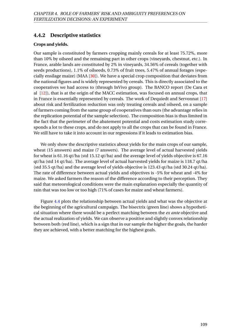
CHAPTER 4. ROLE OF FARMERS’ RISK AND AMBIGUITY PREFERENCES ONFERTILIZATION DECISIONS: AN EXPERIMENT
4.4.2 Descriptive statistics
Crops and yields.
Our sample is constituted by farmers cropping mainly cereals for at least 75.72%, morethan 10% by oilseed and the remaining part in other crops (vineyards, chestnut, etc.). InFrance, arable lands are constituted by 2% in vineyards, 34.56% of cereals (together withseeds productions), 1.1% of oilseeds, 0.73% of fruit trees, 5.47% of annual forages (espe-cially ensilage maize) (MAA [30]). We have a special crop composition that deviates fromthe national figures and is widely represented by cereals. This is directly associated to thecooperatives we had access to (through InVivo group). The BANCO report (De Cara etal [12]), that is at the origin of the MACC estimation, was focused on annual crops, thatin France is essentially represented by cereals. The work of Dequiedt and Servonnat [17]about risk and fertilization reduction was only treating cereals and oilseed, on a sampleof farmers coming from the same group of cooperatives than ours (the advantage relies inthe replication potential of the sample selection). The composition bias is thus limited inthe fact that the perimeter of the abatement potential and costs estimation study corre-sponds a lot to these crops, and do not apply to all the crops that can be found in France.We still have to take it into account in our regressions if it leads to estimation bias.
We only show the descriptive statistics about yields for the main crops of our sample,wheat (15 answers) and maize (7 answers). The average level of actual harvested yieldsfor wheat is 61.16 qt/ha (std 15.12 qt/ha) and the average level of yields objective is 67.16qt/ha (std 14 qt/ha). The average level of actual harvested yields for maize is 118.7 qt/ha(std 35.5 qt/ha) and the average level of yields objective is 123.43 qt/ha (std 30.24 qt/ha).The rate of difference between actual yields and objectives is -5% for wheat and -4% formaize. We asked farmers the reason of the difference according to their perception. Theysaid that meteorological conditions were the main explanation especially the quantity ofrain that was too low or too high (71% of cases for maize and wheat farmers).
Figure 4.4 plots the relationship between actual yields and what was the objective atthe beginning of the agricultural campaign. The bisectrix (green line) shows a hypotheti-cal situation where there would be a perfect matching between the ex ante objective andthe actual realization of yields. We can observe a positive and slightly convex relationshipbetween both (red line), which is a sign that in our sample the higher the goals, the harderthey are achieved, with a better matching for the highest goals.
109

CHAPTER 4. ROLE OF FARMERS’ RISK AND AMBIGUITY PREFERENCES ONFERTILIZATION DECISIONS: AN EXPERIMENT
Figure 4.4 – Relationship between actual and objective yields
We constructed a rate of deviation on the form actual yi el d s−g oal sg oal s in order to observe
the level of deviation on a normalized basis, which allows volume comparisons. Resultsare presented in Figure 4.5.
Figure 4.5 – Deviation rate between actual and objective yields
The average rate is -8.24% (std 0.14%, 37 answers). We can observe that the average
110

CHAPTER 4. ROLE OF FARMERS’ RISK AND AMBIGUITY PREFERENCES ONFERTILIZATION DECISIONS: AN EXPERIMENT
rate of yields objective achievement by crops is most of the time negative, strong for somecrops (ensilage maize especially), and positive for two crops (maize seeds and sunflower).The 2018’s agricultural campaign was particularly difficult for a lot of farmers all over thecountry. We can’t deny that it could have an impact on lot of variables, and maybe alsothose related to uncertainty.
Synthetic nitrogen fertilization.
95.6% of the respondents applied synthetic nitrogen fertilizers on their parcel. The shareof operational costs associated to synthetic nitrogen fertilizers use on the declared parcelsis 26% on average (24 answers). This is important if we set that in general, labor (wage),mechanical soil work (fuel, etc.), seeds, other fertilizers, phytosanitary products and po-tentially irrigation might be contingent operational costs on the same parcel.
The nitrogen balance sheets give the total nitrogen fertilizers application on the parcelduring the agricultural campaign (in kgN/ha). It does not make a lot of sense to observethe general statistics for this variable because it highly depends on the crop, and inter-crop comparisons have no actual interest in our topic. We still can say that the averagelevel of fertilization is around 151 kgN/ha (std 72.5 kgN/ha, 37 non-empty answers) asindicated on Figure 4.6. This graph shows how farmers tend to follow advices from theircooperative agent in terms of fertilization for the annual cropping. We can observe thatfarmers relatively apply as much fertilizers as the advice, except some outliers. We stillcan say that there are more deviations when the advice is higher.
Figure 4.6 – Relationship between actual and adviced fertilization
Reducing the global synthetic nitrogen application balance sheet is an important mit-igation practice. But it relies on the actual nitrogen rates in the soils, and depends on thealternative practice in case of insufficient nitrogen rate. While alternatives (like legume
111

CHAPTER 4. ROLE OF FARMERS’ RISK AND AMBIGUITY PREFERENCES ONFERTILIZATION DECISIONS: AN EXPERIMENT
crop in intermediary cropping) are not always applicable or efficient enough, another ap-proach is to split the applications and to modulate each application in order to optimizethe leaching by crops according to their needs over time, and thus to reduce the loss bynon-absorption and the emission of N2O by volatilization. This is especially the first ap-plication at the beginning of the campaign (during the crop growth cycle) that can besource of modulation, and advisers try to push farmers to put less nitrogen fertilizers atthe beginning and if needed, to compensate with more fertilizer at the next application.Moreover, the first application is associated to much more emissions (Sheriff [37]). Tech-nically, the reduction of fertilization at the first splitting relies on the fact that it can still benitrogenous from the last campaign and the precedent crop if soils are correctly managedbetween campaigns. In another vein, the first application is crucial and source of uncer-tainty if badly implemented: the beginning of the growth cycle is very important for theremaining of the campaign and for the yields goals to be reached (as well as quality goals).Moreover, it can be impossible to make sidedressing applications of nitrogen in the ad-vanced stages of the growing-blooming cycle depending on uncertain water access andfield work conditions, so that risk averse farmers would tend to apply more nitrogen thanrisk neutral farmers at the first application (Sheriff [37]; Bontems and Thomas [8]; Fein-erman et al. [21]). However, the assumption that farmers attribute clear objective profitsdistribution to the fertilization practices is weak, since the issue may fairly be that the un-certainty can be deeper about the future states-of-the-nature, due to the embeddednessof several uncertain bio-physical factors in the forecasts related to sidedressing possibil-ities. We seek to see how splitting is implemented by the farmers from our sample, andalso if it deviates from the advices coming from the cooperative agents, in relationshipwith risk and ambiguity preferences. The average level of fertilization at the first appli-cation is around 50.5 kgN/ha (std 24.7 kgN/ha, 37 non-empty answers). Once again, itdepends a lot on crops and inter-crop comparisons are not our interest. We compute thesame graph than Figure 4.6 for the first application of fertilizer. The same kind of behav-iors is observable in Figure 4.7.
We developed indicators about the degree to which farmers tend to follow advicesin terms of total synthetic nitrogen fertilizers application, of fertilizer application for thefirst application, and for the number of splitting. Farmers’ preferences under uncertaintymay impact the willingness to follow advices, if the assumption of uncertainty associ-ated to their consequences is valid. The two first indicators share the same structure:actual pr acti ce−ad vi ce
ad vi ce . They are a normalized rate of matching, that is negative if farmersput less than advised, positive if they put more, null if they perfectly match the advice.The more they go far from 0, the more the farmer deviated from the advice. The averagerate of matching for the total fertilization is -0.08 (std 0.21, 33 answers), and for the firstapplication it is -0.043 (std 0.28, 23 answers). For the number of splitting and the relatedadvice, that is a relative integer, the indicator is just a difference between the actual num-ber and the advised number. 0.5 means a semi-split: it is a situation where two differentsplittings were possible for the adviser (2 or 3, 4 or 5 for instance), and the farmer hadthe choice. The average number of difference between advices and actual practices is 0.1(std 0.5, 29 answers). 79% of farmers applied exactly what they were told to in terms ofsplitting.
17 respondents have been placed in a "vulnerable zone" for the questioned parcel, aspecific recognition of environmental quality on the parcel and the risk in terms of eco-logical destruction if certain farming practices are used (around 37% but there are a lot of
112

CHAPTER 4. ROLE OF FARMERS’ RISK AND AMBIGUITY PREFERENCES ONFERTILIZATION DECISIONS: AN EXPERIMENT
Figure 4.7 – Relationship between actual and adviced first application
missing answers). This official zoning implies obligation and forbidden practices, espe-cially in terms of nitrogen fertilization. In our sample, the average maximum authorizedquantity of nitrogen fertilization is 154.6 kgN/ha (16 answers). 20.6% declared havinga mandatory fertilization method, such as using only organic fertilizer, liquid product,ovine manure (34 answers). These statistics give an idea of the weight of regulation onrespondents, despite the regular lack of answers to these questions.
Other practices and characteristics.
We asked farmers who applied organic fertilizer (manure for instance) on the parcel howthey did take into account the amount of nitrogen contained in this product. Among the34 answers we collected, 35.56% only used the reference table (very generalist in terms ofinformation), 20% only used an analysis of the product (the most precise source of infor-mation), and 4.4% both, while 15.56% did not take the amount of nitrogen into account.This application of organic-based nitrogen was taken into account for the synthetic nitro-gen application by 90.32% of respondents (31 answers). Thus, we can see that the preciselevel of nitrogen that is applied is not always known by farmers before they apply fertilizeron their parcels. 59.38% of farmers that applied organic fertilizer buried it through tillage(32 answers). Only 4.9% of farmers did not apply any nitrogen fertilizer. 56% applied bothon their parcel, while 39% applied only synthetic fertilizer and none of the farmers ap-plied only organic fertilizers (41 answers).
Respondents come from Drôme (31.71%), Meuse (21.95%), Tarn (21.95%), CharenteMaritime (12.20%), Isère (7.32%), and Meurthe (4.88%). We can see that we have a widegeographic dispersion with a non-homogeneous composition. This presents the advan-tage of getting us a control for some fixed local characteristics that can be catched throughthe department membership (or the town, that we know too). The disadvantage is that we
113
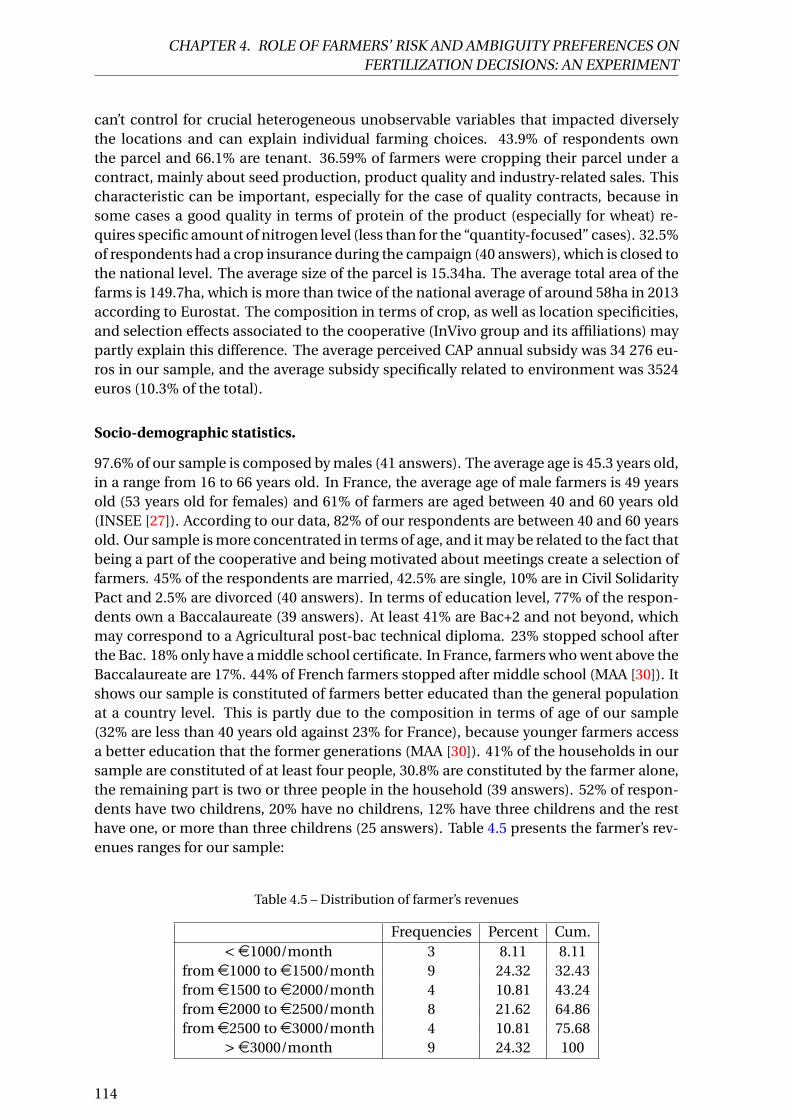
CHAPTER 4. ROLE OF FARMERS’ RISK AND AMBIGUITY PREFERENCES ONFERTILIZATION DECISIONS: AN EXPERIMENT
can’t control for crucial heterogeneous unobservable variables that impacted diverselythe locations and can explain individual farming choices. 43.9% of respondents ownthe parcel and 66.1% are tenant. 36.59% of farmers were cropping their parcel under acontract, mainly about seed production, product quality and industry-related sales. Thischaracteristic can be important, especially for the case of quality contracts, because insome cases a good quality in terms of protein of the product (especially for wheat) re-quires specific amount of nitrogen level (less than for the “quantity-focused” cases). 32.5%of respondents had a crop insurance during the campaign (40 answers), which is closed tothe national level. The average size of the parcel is 15.34ha. The average total area of thefarms is 149.7ha, which is more than twice of the national average of around 58ha in 2013according to Eurostat. The composition in terms of crop, as well as location specificities,and selection effects associated to the cooperative (InVivo group and its affiliations) maypartly explain this difference. The average perceived CAP annual subsidy was 34 276 eu-ros in our sample, and the average subsidy specifically related to environment was 3524euros (10.3% of the total).
Socio-demographic statistics.
97.6% of our sample is composed by males (41 answers). The average age is 45.3 years old,in a range from 16 to 66 years old. In France, the average age of male farmers is 49 yearsold (53 years old for females) and 61% of farmers are aged between 40 and 60 years old(INSEE [27]). According to our data, 82% of our respondents are between 40 and 60 yearsold. Our sample is more concentrated in terms of age, and it may be related to the fact thatbeing a part of the cooperative and being motivated about meetings create a selection offarmers. 45% of the respondents are married, 42.5% are single, 10% are in Civil SolidarityPact and 2.5% are divorced (40 answers). In terms of education level, 77% of the respon-dents own a Baccalaureate (39 answers). At least 41% are Bac+2 and not beyond, whichmay correspond to a Agricultural post-bac technical diploma. 23% stopped school afterthe Bac. 18% only have a middle school certificate. In France, farmers who went above theBaccalaureate are 17%. 44% of French farmers stopped after middle school (MAA [30]). Itshows our sample is constituted of farmers better educated than the general populationat a country level. This is partly due to the composition in terms of age of our sample(32% are less than 40 years old against 23% for France), because younger farmers accessa better education that the former generations (MAA [30]). 41% of the households in oursample are constituted of at least four people, 30.8% are constituted by the farmer alone,the remaining part is two or three people in the household (39 answers). 52% of respon-dents have two childrens, 20% have no childrens, 12% have three childrens and the resthave one, or more than three childrens (25 answers). Table 4.5 presents the farmer’s rev-enues ranges for our sample:
Table 4.5 – Distribution of farmer’s revenues
Frequencies Percent Cum.<e1000/month 3 8.11 8.11
frome1000 toe1500/month 9 24.32 32.43frome1500 toe2000/month 4 10.81 43.24frome2000 toe2500/month 8 21.62 64.86frome2500 toe3000/month 4 10.81 75.68
>e3000/month 9 24.32 100
114

CHAPTER 4. ROLE OF FARMERS’ RISK AND AMBIGUITY PREFERENCES ONFERTILIZATION DECISIONS: AN EXPERIMENT
4.4.3 Pairwise correlations and marginal impact estimations
Correlations.
We performed pairwise correlations estimations (Pearson or Spearman) between all ourmeasures of risk and ambiguity attitudes with interest variables: the total level of nitro-gen fertilization, the level of fertilization at the first application, the number of splittingin fertilizers application, the rate of differential between the total advised application andwhat has been actually applied, the rate of differential between the actual and advisedfirst application, and the rate of differential between the number of advised and actualsplitting. We found no significant correlations with the Pearson coefficient applied oncontinuous variables. The Pearson coefficient fails at estimating correlation coefficientfor ordinal or categorical variables. The Spearman rank-order coefficient is suited to esti-mate correlation coefficients with categorical variables. We found only one almost signif-icant (p-value = 0.13) positive Spearman correlations between the NRC (ambiguity) andthe level of fertilization at the first application (Spearman = 0.28). This would be the signthat farmer applies more nitrogen at the first fertilization splitting when they are ambi-guity averse. Sheriff [37], and Bontems and Thomas [8] show that sidedressing nitrogenfertilization can be cost-efficient (better use of input) but depends on the propensity offarmers to take the risk that future natural conditions can prevent them from doing otherapplications after the first splitting. We find a negative relationship between our categor-ical variable of risk aversion and the number of fertilization splitting, but the coefficientis not significant. The main result with the Spearman rank-order coefficient shows a newrelationship: ambiguity aversion leads farmers who agreed to split applications to applymore at the first stage in a situation where they are totally uncertain about what the futureconditions will be. That can be the sign that when the risk of splitting is taken, ambiguityaversion encourages farmers to hedge against the probabilistic uncertainty that they areexposed to. However, lot of other factors can explain that phenomenon, that we can’t testsince we are not ceteris paribus. Moreover, the low level of observations and the unbal-anced nature of the answers between respondents and questions make the estimationsand tests limited.
Taking into account sampling design in regressions.
The observations of our sample were not individually selected: we performed our experi-ment randomly on the farmers that we had at our disposal in usual meetings that occuredin the cooperatives. However, the probability of being “selected” in our sample directlydepends on individual characteristics of the respondents (crop, soil, etc.) that lead themto be a part of these experiment groups and can simultaneously impact individuals’ de-cisions. Those characteristics are heterogeneously repeated in the sample, so that thecomposition of the sample is not the same as for the total population. Any regressionthat would be runned without correcting for these sampling selections would attributefalse phenomenons to the whole population of farmers, while the results would be onlyaccurate for the sample at stake. Ignoring selection weight can thus lead to biases in es-timation, and it is possible to fix this issue by attributing probability weight to each ob-servation. Finding the proper variables that can be used to make good sampling weightsdepends on the available data and on the assumption we can make about the probabilityof selection. The crop the farmers choose on their parcel seems to us a good weightingvariable, since the composition of our sample is widely determined by crops and targetingcooperative that work with annual non-perennial crop was one of our selection criteria.
115

CHAPTER 4. ROLE OF FARMERS’ RISK AND AMBIGUITY PREFERENCES ONFERTILIZATION DECISIONS: AN EXPERIMENT
The composition bias can be important, since two main crops compose our sample andwear specific agronomic and economic characteristics (wheat and maize). Moreover, thisquestion has been generally well-filled by respondents. Adding probability weighting isfeasible with Stata: the dependent and independent variables of each row is multiplied bya weight that corresponds to the inverse of the probability of having put each crop on theparcel and the variance-covariance matrix is estimated through a robust sandwich esti-mator. The more a crop represents a big proportion in the sample, the smallest will be themultiplied factor.
Our observations were collected by group (local cooperatives) so that there can be cor-relation between error terms between observations in a same group, leading to a failureof the homoskedasticity assumption. These clustering can be taken into account in theregressions by applying adjustment weighting coefficients to subgroups standard errorscovariance matrix in order to correct heteroskedasticity. We can assume that the localcooperative groups from which the farmers come are natural clusters among which re-spondents are concentrated, and some unobservable phenomena can affect the groupuniformly. This subgroup catches correlation between behaviors as well as a part of ex-ogenous natural hazards. We can also use a White [39] heteroskedasticity consistent stan-dard errors estimation in order to fix for heteroskedasticity issues, but it does not allowfor clustered variability to be corrected, and the adjustment is at the individual level. Wewill compare both.
Regressions results.
We will only comment regression with significant coefficients. Given the limited numberof observations, most of the relevant regressions were the ones with at least thirty obser-vations. This is the higher average number of observations we obtained. Given the lownumber of degrees of freedom, we limited our regressions to one independent variable.
Table 4.6 – Total fertilization
VARIABLES
Risk lovers -28.25 -50.60 -50.60(54.07) (41.58) (49.03)
Risk averse -58.16 -48.84** -48.84***(41.43) (19.57) (5.471)
Ambiguity lovers -12.25 18.80 18.80(32.17) (28.91) (14.96)
Ambiguity averse -30.70 -14.52 -14.52(37.48) (40.08) (21.10)
NSC 3.754 6.827 6.827(6.278) (4.775) (5.393)
NRC -3.424 -6.235 -6.235(6.794) (6.461) (4.430)
Constant 191.2*** 186.9*** 186.9*** 157.4*** 142.4*** 142.4*** 122.7*** 103.5*** 103.5* 162.6*** 177.0*** 177.0***(38.24) (8.863) (4.501) (22.75) (25.72) (8.803) (39.03) (34.51) (35.30) (36.34) (33.83) (22.89)
Weighting (crop) No Yes Yes No Yes Yes No Yes Yes No Yes YesClustering (cooperative) No No Yes No No Yes No No Yes No No Yes
Observations 31 31 31 31 31 31 31 31 31 31 31 31R-squared 0.074 0.047 0.047 0.023 0.031 0.031 0.012 0.042 0.042 0.009 0.030 0.030F 1.121 3.595 117.5 0.336 0.610 1.590 0.357 2.045 1.603 0.254 0.931 1.982p-Fisher 0.340 0.0408 0.00142 0.717 0.550 0.338 0.555 0.163 0.295 0.618 0.342 0.254
Standard errors in parentheses*** p<0.01, ** p<0.05, * p<0.1
We can see in Table 4.6 that in the most robust regressions that we have (third col-umn), the fact to be in the risk averse category leads to a significant lower level of total
116

CHAPTER 4. ROLE OF FARMERS’ RISK AND AMBIGUITY PREFERENCES ONFERTILIZATION DECISIONS: AN EXPERIMENT
Table 4.7 – Fertilization at the first splitting
VARIABLES
Risk lovers 1.750 1.825 1.825(19.35) (6.614) (7.242)
Risk averse -0.207 -4.310 -4.310(14.82) (6.873) (5.037)
Ambiguity lovers -3.667 6.471 6.471(8.682) (8.172) (6.882)
Ambiguity averse 3.762 4.886 4.886(10.11) (12.61) (2.738)
NSF 0.732 1.529 1.529(2.171) (1.567) (1.198)
NRC 2.094 1.422 1.422*(1.796) (2.005) (0.527)
Constant 51.25*** 53.14*** 53.14*** 48.67*** 45.44*** 45.44*** 47.07*** 41.02*** 41.02*** 37.76*** 41.08*** 41.08***(13.68) (3.747) (4.580) (6.139) (6.655) (2.332) (13.50) (10.77) (6.668) (9.606) (10.03) (4.301)
Weighting (crop) No Yes Yes No Yes Yes No Yes Yes No Yes YesClustering (cooperative) No No Yes No No Yes No No Yes No No Yes
Observations 31 31 31 31 31 31 31 31 31 31 31 31R-squared 0.001 0.009 0.009 0.019 0.019 0.019 0.004 0.020 0.020 0.045 0.018 0.018F 0.00873 0.318 0.537 0.277 0.315 8.685 0.114 0.953 1.628 1.360 0.503 7.282p-Fisher 0.991 0.730 0.632 0.760 0.732 0.0565 0.738 0.337 0.292 0.253 0.484 0.0739
Standard errors in parentheses*** p<0.01, ** p<0.05, * p<0.1
fertilization compared to the reference category of risk neutral farmers (coeff. = -48.84significant at the 1% level). Reversely, the fact to be more ambiguity averse (NRC) has apositive marginal impact on the quantity of nitrogen fertilizers applied at the first split(coeff. = 1.422 significant at the 10% level). These results have to be interpreted simulta-neously.
The first one indicates a phenomenon that is symmetric to numerous common as-sumptions about the positive impact of risk aversion on nitrogenous fertilization. Whilethe role of risk aversion on fertilization, as we saw in the literature review, is not clear-cutand depends on the risk-increasing or decreasing nature of the input (and thus dependson the natural states-of-the-nature in terms of meteorological conditions, and comple-mentarity with water and pesticide uses), nitrogen fertilizers seem to be not consideredas a risk-decreasing input in our sample. This lowers the assumption that risk aversioncan be a barrier to adoption of practices that reduces the total quantity of fertilizers use,because it reversely looks like a driver of reduction. However, it is notable that the riskaversion variable at stake is the categorical one: the reference category that we choose forcomparison is the category 2, for risk neutrality. The coefficient is thus the average levelof fertilizers of risk averse farmers in general compared to risk neutral farmers in general.
The second result is the most original. Ambiguity aversion leads to put more fertilizersat the first application split (see Table 4.7), which is equivalent to say that having an aver-sion for making bets on outcome whose probabilistic distribution is uncertain encouragesfarmers to hedge against future possible nitrogen lacks. We interpret this result as follows:if cooperative agents ask farmers to split their application, the first application is the mostcrucial, not only because it happens at the beginning of the growing stage for the crop, butespecially because the farmer does not know if it will be possible for her to fertilize againat the future stages, because future states-of-the-nature are deeply uncertain. The possi-bility to make future splittings is dependent on this inability to make complete forecastsabout entangled natural conditions. If we want to connect more the interpretation to thelotteries experiment, we can say that the ambiguity averse farmers insure themselves by
117

CHAPTER 4. ROLE OF FARMERS’ RISK AND AMBIGUITY PREFERENCES ONFERTILIZATION DECISIONS: AN EXPERIMENT
putting more fertilizers at the first splitting, which is exactly the thing cooperative agentsdo not want them to do, because they prefer to bet on a risky practice than an ambiguousone5. That would be the sign that the result confirms the risk-increasing nature of fertil-izers, but farmers are sufficiently ambiguity averse so that they prefer to bear this risk, inorder to cover themselves compared to the ambiguous situation. However, this impact ismuch smaller than the negative impact of risk aversion on total fertilization. Moreover,splitting practices induce dynamic evaluation of profits and optimal input uses, as shownin Bontems and Thomas [8], which implies other potential explanations, like informationvalue. We do not test for that in this study. The benefits from splitting is, according toBontems and Thomas [8], to allow the farmers to gather information about the true nitro-gen needs of the crops and to be more efficient in their first and sidedressing application,thus reducing the production costs. We show in this study that ambiguity aversion mayimpact the total benefits from information value, and is a complementary driver of fertil-ization decisions.
The low number of observation for each regression (31) nuances our results. Addingcontrol variables for crops (17 modalities), soil quality (21 modalities), precedent crops(22 modalities), interactions between risk and ambiguity preferences, differences betweenactual yields and yields goals and the perception of experienced risks at the last campaignby farmers, and several controls for agricultural practices and socioeconomic and demo-graphic variables would produce more robust results and limit the biases that we mayexperience. Because each modality of the categorical variables represents a covariate, thenecessary number of observations would have to be significantly higher. The dependentvariables related to fertilization being directly explained by obvious variables like the cropthat has been put on the parcel by the farmers or the soil quality, which are informationthat we asked in the questionnaire, it would be crucial to make our regression with thesecontrols. This is an important caveat of our econometric analysis.
The indicators about the degree to which farmers tend to follow advices in terms oftotal synthetic nitrogen fertilizers application, of fertilizer application for the first appli-cation, and for the number of splitting were not sufficiently matched with answer aboutrisk and ambiguity preferences, so that a too limited number of observations were gather-able. It reinforce our willingness to have more observations.
4.5 Conclusion
We implemented an experiment on farmers in collaboration with their cooperative group(InVivo group) in order to test on real data our main assumption: uncertainty may be abarrier to nitrogen fertilization reduction. We test two levels of preferences toward un-certainty, risk attitudes (known probability) and ambiguity attitudes (unknown probabil-ity). In the scope of our goal to estimate the interactions between those measures andthe mitigation potential associated to fertilizer reduction, we seeked to test the role ofthese individual behavioral attitudes on diverse practices related to fertilization, aboutthe fertilization practices directly (global level of fertilizer, level of fertilization at the firstsplitting, number of splittings) and the farmers’ willingness to follow advices from theircooperative agents who try to lead them toward less emitting production practices. Wealso planned to estimate the role of several agricultural, regulatory and socioeconomic
5Adding variables of interactions between risk and ambiguity preferences is an extension we plan to do.
118

CHAPTER 4. ROLE OF FARMERS’ RISK AND AMBIGUITY PREFERENCES ONFERTILIZATION DECISIONS: AN EXPERIMENT
characteristics, and their embedded with uncertainty preferences, on fertilization prac-tices and propensity to follow advices.
We found that our respondents were mostly risk averse, and ambiguity neutral or in-clined. Our measures are closed to some previous studies on farmers. The representa-tiveness of our sample in terms of crops is low (with comparison to French farmers) butis closed from the previous studies about nitrogen fertilization reduction, which oftentest the same kind of crops, cereals and oilseeds. The last campaign were globally not agood year for our respondents, who slightly failed on average to reach their yields goals.Our respondents did not follow perfectly what was advised in terms of fertilization, andan important part of them has to be in compliance with fertilization regulatory rules ontheir parcel. They present some important statistical differences with the national farm-ers population, in terms of size of farm (bigger), age (younger) and education (more edu-cated).
We performed OLS regressions with considerations of sampling design in order to pro-duce the most robust estimations as possible. We found significant marginal impacts onlyfor two dependent variables (when sample weights and clustering are introduced), the to-tal quantity of nitrogen fertilizer use, and the quantity of fertilizer use at the first splitting.Being risk averse is associated to a lower level of total fertilization (-48.8 kgN/ha on aver-age) with respect to the reference category (risk neutrality). This result is interesting butdifficult to analyze, because it can be the sign that nitrogen fertilizers are perceived asrisk-increasing by farmers, or risk-decreasing (or neutral) but the global level of risk wereperceived as very low by farmers who self-insure with fertilizers. It could be the sign ofdiverse water and fertilizer use characteristics (Feinerman et al. [21]) and interaction be-tween pest invasion risk with good growing conditions and crops growth level related tofertilizer use (Horowitz and Lichtenberg [26]). However, we can say that the total level offertilization may be always associated to yields goals and agricultural knowledge of farm-ers for which they might have an objective probabilistic “mapping”, and a clear ex antestochastic production plan for the whole campaign. The second main result is the posi-tive marginal impact of ambiguity aversion (NRC variable) on the level of fertilization atthe first splitting (+1.42kg/ha for each higher level of risky choice). While this result isunique to our knowledge, it echoes some previous researches that highlighted the deepuncertainty that lay behind the splitting practice. Indeed, splitting fertilization is a goodway to adapt the fertilizer application to the crops’ needs, but it relies on technical fea-sibility of postponed applications, which itself directly depends on unpredictable pedo-meteorological conditions, and their short-term deeply uncertain fluctuations. Uncertainevolution of states-of-the-nature can’t be ex ante forecasted at the time of the first applica-tion, but the farmer can have subjective priors and be more or less pessimistic about whatcan be expected. In this scope, ambiguity aversion impacts positively the level of fertil-ization at the first application. However, the marginal impact is low, implying that eventhe global effect is negligible compared to the first result. The net total estimated impactof our preferences measures on the total fertilization is negative. Moreover, the first re-sult is significant because of sampling weight, while the second is significant because ofclustered heterosckedastic-robust standard errors. The first case is not surprising. On theother hand, the second fact indicates that the significance of the result depends on theconsideration of specific cluster-dependent unobservable variables, like very local fluc-tuations and characteristics. It is interesting because it can echo our interpretation aboutthe NRC result, that ambiguity associated to the first splitting is embedded in the indi-
119

CHAPTER 4. ROLE OF FARMERS’ RISK AND AMBIGUITY PREFERENCES ONFERTILIZATION DECISIONS: AN EXPERIMENT
vidual deep uncertainty about technical and natural feasibility of postponed splittings,which may be essentially local-specific and thus, partly shared by farmers from a givencooperative. In another vein, it is possible that the cluster-corrected standard errors fixesunobserved shocks on group-variations that are directly related to the differences thatcould have appear in the measurement processes between cooperative. While we triedto make exactly the same experiment on each farmers, it may have had slight differenceswhich provoked group-specific measurement errors (day, time in the day, context etc.).This is specific to field experiments compared to laboratory experiments.
We have several external and internal validity issues. We are limited by the number ofrespondents and the subsequent number of valid answers in our estimations. This limitsthe external validity of our results. Our experiment may be seen as a pilot for a wider ex-periment, in order to observe if our current results are robust or not to all the necessarycontrols. In terms of internal validity, it would be an interesting extension associated tothe fact that we do not test for time preferences impact in this study. Time preferences ex-plain choices at each step of the production, as well as decisions in terms of practices andproduction goals. Secondly, the use of the MPL procedure entails advantages and caveats.These lotteries rely on the widely accepted assumption of a CRRA (power) utility function,and its form (chained lotteries with switching point) allows for the precise measurementof the level of risk aversion on the continuous distribution of gains. Moreover, its wideuse in the literature allows for a good level of comparativeness of our results. The maincaveats entangle the limit in identification of the actual preferences of the respondent.First, if the preferences of the agent do not follow a CRRA utility function, or more gen-erally, if the individual has preferences not in line with expected utility framework, thenthe method is not relevant. This would lead to the risk that our subsequent regressionswould have a limited internal invalidity and thus, limited results. Second, as we men-tioned in the literature review, some critics have been developed by Drichoutis and Lusk[18]. However, these caveats did not prevent several studies to produce creditable results(see literature review).
There are two main implications in terms of public policies. First, this study partlyshows that risk and ambiguity attitudes impact abatement costs associated to nitrogenfertilization reduction. While ambiguity aversion is a hidden costs of innovative fertiliza-tion practices like splitting, risk aversion can be a "hidden abatement benefit" for globalreduction of nitrogen application. We can conclude that these phenomena question theoptimality of flat rate subsidies. Fluctuations in production conditions can make fluctu-ate the abatement costs mechanically, and subsidies aiming at offsetting potential lossesfrom reduction can become a windfall for farmers that would, in their majority, adjusttheir use of fertilizer by themselves. This feature induces a questioning of usual recom-mendations under risk consideration, like subsidized crop insurance that would coveryields risk and by this mean, encourages farmers to lower their fertilization: it dependson the interaction between nitrogen fertilizers and the environment they are applied in,and the crop, thus it can even have counter-productive effects on N2O mitigation (Sheriff[37]). If we get back to the work of Bontems and Thomas [7], we can say that fertilizationsplitting wears a huge benefit in terms of information value. This explains why farmerswould be not so reluctant to adopt this practice. However, if ambiguity aversion increasesthe level of application at the first splitting and thus, increases emissions, it could be goodto rather reducing uncertainty through generalized soil testing in order to securize infor-mation while developing new methods to ensure that sidedressing will be certainly mak-
120

CHAPTER 4. ROLE OF FARMERS’ RISK AND AMBIGUITY PREFERENCES ONFERTILIZATION DECISIONS: AN EXPERIMENT
able later in the campaign. Trials can also be offered under diverse forms in order toimprove farmers knowledges about the reaction of crops to these new forms of nitrogenmanagement over the growing period.
121

CHAPTER 4. ROLE OF FARMERS’ RISK AND AMBIGUITY PREFERENCES ONFERTILIZATION DECISIONS: AN EXPERIMENT
Bibliography
[1] B.L. Barham, J.P. Chavas, D. Fitz, V.R. Salas, and L. Schechter. The roles of risk andambiguity in technology adoption. Journal of Economic Behavior & Organization,97:204–218, 2014. 103, 107
[2] R. Battalio, J. Kagel, and K. Jiranyakul. Testing between alternative models of choiceunder uncertainty: Some initial results. Journal of Risk and Uncertainty, 3(1):2550–,1990. 104
[3] J. Beattie and G. Loomes. The impact of incentives upon risky choice experiments.Journal of Risk and Uncertainty, 14:155–168, 1997. 104
[4] H.P. Binswanger. Risk attitudes of rural households in semi-arid tropical India. Eco-nomic and Political Weekly, pages A49–A62, 1978. 102
[5] H.P. Binswanger. Attitudes toward risk: Experimental measurement in rural India.American Journal of Agricultural Economics, 62:395–407, 1980.
[6] G. Bocquého, F. Jacquet, and A. Reynaud. Expected utility or prospect theory max-imisers? assessing farmers’ risk behaviour from field-experiment data. EuropeanReview of Agricultural Economics, 41:135–172, 2014. 102
[7] Bontems and Thomas. Information value and risk premium in agricultural produc-tion: the case of split nitrogen application for corn. American Journal of AgriculturalEconomics, 82(1):59–70, 2000. 120
[8] P. Bontems and A. Thomas. Information value and risk premium in agricultural pro-duction: The case of split nitrogen application for corn. American Journal of Agricul-tural Economics, 82:59–70, 2000. 101, 112, 115, 118
[9] D. Bougherara, X. Gassmann, L. Piet, and A. Reynaud. Structural estimation of farm-ers’ risk and ambiguity preferences: A field experiment. European Review of Agricul-tural Economics, 44(5):782–808, 2017. 102, 107
[10] M. Brunette, L. Cabantous, S. Couture, and A. Stenger. The impact of governmen-tal assistance on insurance demand under ambiguity: A theoretical model and anexperimental test. Theory and Decision, 75:153–174, 2013. 104
[11] M. Brunette, J. Foncel, and E. Kéré. Attitude towards risk and production decision :An empirical analysis on french private forest owners. Environmental Modeling andAssessment, 22(6):563–576, 2017. 100, 104
[12] De Cara, Stéphane (a); Delame, Nathalie (a); Dequiedt, Benjamin; Camuel, Alexan-dre. BANCO Consortium technical report, 1(19):7–42, 2017. 109
[13] C.F. Camerer and R. Hogarth. The effects of financial incentives in experiments: Areview and capital-labor-production framework. Journal of Risk and Uncertainty, 1(19):7–42, 1999. 104
[14] S. Chakravarty and J. Roy. Recursive expected utility and the separation of attitudestowards risk and ambiguity: An experimental study. Theory and Decision, 66(3):199–228, 2009. 102, 103
122

CHAPTER 4. ROLE OF FARMERS’ RISK AND AMBIGUITY PREFERENCES ONFERTILIZATION DECISIONS: AN EXPERIMENT
[15] CITEPA. Inventaire secten, 2019. URL https://www.citepa.org/fr/activites/
inventaires-des-emissions/secten. 100
[16] T. Le Cotty, E. Maître d’Hôtel, R. Soubeyran, and J. Subervie. Linking risk aversion,time preference and fertiliser use in burkina faso. The Journal of Development Stud-ies, 54(11):1991–2006, 2018. 102
[17] B. Dequiedt and E. Servonnat. Risk as a limit or an opportunity to mitigate ghg emis-sions? the case of fertilisation in agriculture. Working Papers Climate Economic Chair(CEC), 1606(3):–, 2016. 101, 109
[18] A.C. Drichoutis and J.L. Lusk. What can multiple price lists really tell us about riskpreferences? Journal of Risk and Uncertainty, 53(2-3):89–106, 2016. 120
[19] C.C. Eckel and P.J. Grossman. Forecasting risk attitudes: An experimental study usingactual and forecast gamble choices. Journal of Economic Behavior & Organization,68(1):1–7, 2008. 102
[20] J. Engle-Warnick, J. Escobal, and S. Laszlo. Ambiguity aversion as a predictor of tech-nology choice: Experimental evidence from peru. CIRANO - Scientific Publications,2007s-01, 2007. 103
[21] Eli Feinerman, E Kwan Choi, and Stanley R Johnson. Uncertainty and split nitrogenapplication in corn production. American Journal of Agricultural Economics, 72(4):975–985, 1990. 112, 119
[22] M. Gandorfer, D. Pannell, and A. Meyer-Aurich. Analyzing the effects of risk anduncertainty on optimal tillage and nitrogen fertilizer intensity for field crops in ger-many. Agricultural Systems, 104(8):615–622, 2011. 101
[23] A.K.A. Ghadim, D.J. Pannell, and M.P. Burton. Risk, uncertainty, and learning inadoption of a crop innovation. Agricultural Economics, 33(1):1–9, 2005. 102
[24] D. Hellerstein, N.A. Higgins, and J. Horowitz. The predictive power of risk preferencemeasures for farming decisions. European Review of Agricultural Economics, 40(5):807–833, 2013. 103
[25] C.A. Holt and S.K. Laury. Risk aversion and incentive effects. The American EconomicReview, 92(5):1644–1655, 2002. 102, 103
[26] John K Horowitz and Erik Lichtenberg. Risk-reducing and risk-increasing effects ofpesticides. Journal of Agricultural Economics, 45(1):82–89, 1994. 119
[27] INSEE. Tableaux de l’économie française, 2018. URL https://www.insee.fr/fr/
statistiques/. 114
[28] H.D. Leathers and J.C. Quiggin. Interactions between agricultural and resource pol-icy: The importance of attitudes toward risk. American Journal of Agricultural Eco-nomics, 73(3):757–764, 1991. 101
[29] E.M. Liu. Time to change what to sow: Risk preferences and technology adoptiondecisions of cotton farmers in China. The Review of Economics and Statistics, 95:1386–1403, 2013. 103
123
CHAPTER 4. ROLE OF FARMERS’ RISK AND AMBIGUITY PREFERENCES ONFERTILIZATION DECISIONS: AN EXPERIMENT
[30] MAA. Agreste, la statistique, l’evaluation et la prospective agricole. 2019. 109, 114
[31] M. Monjardino, T. McBeath, J. Ouzman, R. Llewellyn, and B. Jones. Farmer risk-aversion limits closure of yield and profit gaps: A study of nitrogen managementin the southern Australian wheatbelt. Agricultural Systems, 137:108–118, 2015. 101
[32] G. Moschini and D.A. Hennessy. Uncertainty, risk aversion, and risk management foragricultural producers. Handbook of Agricultural Economics,in: B. L. Gardner & G. C.Rausser (ed.), Handbook of Agricultural Economics, edition 1, 1(2):88–153, 2001. 101
[33] Sylvain Pellerin, Laure Bamière, Denis Angers, Fabrice Béline, Marc Benoit, Jean-Pierre Butault, Claire Chenu, Caroline Colnenne-David, Stephane De Cara, NathalieDelame, Michel Doreau, Pierre Dupraz, Philippe Faverdin, Florence Garcia-Launay,Melynda Hassouna, Catherine Hénault, Marie-Helene Jeuffroy, Katja Klumpp, Au-rélie Metay, Dominic Moran, Sylvie Recous, Elisabeth Samson, Isabelle Savini, andLenaïc Pardon. Quelle contribution de l’agriculture française à la réduction desémissions de gaz à effet de serre? Potentiel d’atténuation et coût de dix actions tech-niques. Technical Report hal-01186943, HAL, 2013. 100
[34] R.D. Pope and R.A. Kramer. Production uncertainty and factor demands for the com-petitive firm. Southern Economic Journal, 46(2):489–502, 1979. 101
[35] A. Reynaud and S. Couture. Stability of risk preference measures: Results from a fieldexperiment on French farmers. Theory and Decision, 73:203–221, 2012. 102, 104, 107
[36] J. Roosen and D.A. Hennessy. Tests for the role of risk aversion on input use. Ameri-can Journal of Agricultural Economics, 85(1):30–43, 2003. 101
[37] G. Sheriff. Efficient waste? why farmers over-apply nutrients and the implications forpolicy design. Applied Economic Perspectives and Policy, 27(4):542–557, 2005. 101,112, 115, 120
[38] D. Stuart, R.L. Schewe, and M. McDermott. Reducing nitrogen fertilizer applicationas a climate change mitigation strategy: Understanding farmer decision-making andpotential barriers to change in the US. Land Use Policy, 36(1):210–218, 2014. 101
[39] H. White. A heteroskedasticity-consistent covariance matrix estimator and a directtest for heteroskedasticity. Econometrica, 48(4):817–838, 1980. 116
[40] M. Wik, T.A. Kebede, O. Bergland, and S.T. Holden. On the measurement of risk aver-sion from experimental data. Applied Economics, 36(21):2443–2451, 2004. 104
124

Appendices
125


The ten-paired lottery-choice
Table 8 – The ten-paired lottery-choice decisions under risk
Decisions Option A Option BProba. Payoff Proba. Payoff Proba. Payoff Proba. Payoff
1 10% e 7 90% e 5 10% e 13 90% e 02 20% e 7 80% e 5 20% e 13 80% e 03 30% e 7 70% e 5 30% e 13 70% e 04 40% e 7 60% e 5 40% e 13 60% e 05 50% e 7 50% e 5 50% e 13 50% e 06 60% e 7 40% e 5 60% e 13 40% e 07 70% e 7 30% e 5 70% e 13 30% e 08 80% e 7 20% e 5 80% e 13 20% e 09 90% e 7 10% e 5 90% e 13 10% e 0
10 100% e 7 0% e 5 100% e 13 0% e 0
Table 9 – The ten-paired lottery-choice decisions under ambiguity
Decisions Option A: urn A Option B: urn BIn urn A, the distribution of In urn B, the distributionballs is 5 black and 5 white of balls is not known
Chosen color Chosen color Chosen color Chosen colorobtained not obtained obtained not obtained
1 e 13 e 0 e 9 e 02 e 12 e 0 e 9 e 03 e 11 e 0 e 9 e 04 e 10 e 0 e 9 e 05 e 9 e 0 e 9 e 06 e 8 e 0 e 9 e 07 e 7 e 0 e 9 e 08 e 6 e 0 e 9 e 09 e 4 e 0 e 9 e 0
10 e 2 e 0 e 9 e 0
Questionnaire
Survey on the use of synthetic nitrogen fertilizers
The survey you are going to participate aims at studying the climate change mitigationmeasures of the French agricultural sector. In particular, the survey focuses on farmers’fertilization decisions. Nitrogen fertilization is one of the main greenhouse gas emissionsin the agricultural sector. The aim is to improve the understanding and determinantsof fertilization decisions, particularly by focusing on an economic parameter reflectingindividual preferences for risky choices.
This survey is conducted as part of a joint project between the INRA (National In-stitute for Agronomic Research), the Climate Economics Chair (CEC), and InVivo. Morespecifically, this work is part of a thesis in Economics, conducted within INRA.
The questionnaire will consist of three parts. In the first part, it will be necessary tomake hypothetical choices between two options. These choices will help measure your
127

individual attitude towards risk. This method is widely used in economics to reveal toindividuals their preferences for more or less risky situations. The second part will becomposed of questions relating to your management decisions and, more particularly,fertilization. The final part of the survey will focus on your socio-economic characteris-tics.
There are no good or bad answers during the survey, just different behaviors to ob-serve. For the purposes of the survey, you must answer all the questions. The confiden-tiality of the information contained in this questionnaire is ensured by the anonymity ofthe respondent. Your answers will remain confidential. The results will be presented insynthetic form in scientific publications with scrupulous respect for the anonymity of therespondents. Once the data is processed, it will be returned to you individually and youcan compare your results to the average of our sample and your cooperative.
The lack of communication between participants is a guarantee of success. We askyou not to discuss with other participants during the survey.
1st part: Choice between two optionsThis first part is composed of two series of 10 decisions represented by two tables.All questions correspond to fictitious situations for which we ask you to answer as if
you were facing a real situation, taking the necessary time to choose the answers that bestcorrespond to your preferences.
First table:For each of the 10 decisions (lines) you must choose which of the two options (A or B) youprefer. Let’s take an example. Decision 1 of the table reads as follows:- Option A: gete7 with 10% chance ore5 with 90% chance.- Option B: gete13 with 10% chance ore0 with 90% chance.This decision 1 can also be represented in the form of a circular graph as well:
13€
10%
5€
90%
7€
10%
0 €
90%
The following decisions read in the same way, only the probabilities associated withearnings change. Please complete the boxes below the table.
- I choose option A for decisions 1 to�.You can answer with a number between 1 and 10. If you choose 3 it implies that option A is chosen for the
first three lines, then B for the following ones. If you choose 1 it implies that you choose A only for the first
line, and B for the others. If you do not put anything that implies that you choose B for all lines: you will
have to answer 1 in the next question.
- I choose option B for decisions� at 10.
128

Decisions Option A Option BProba. Payoff Proba. Payoff Proba. Payoff Proba. Payoff
1 10% e 7 90% e 5 10% e 13 90% e 02 20% e 7 80% e 5 20% e 13 80% e 03 30% e 7 70% e 5 30% e 13 70% e 04 40% e 7 60% e 5 40% e 13 60% e 05 50% e 7 50% e 5 50% e 13 50% e 06 60% e 7 40% e 5 60% e 13 40% e 07 70% e 7 30% e 5 70% e 13 30% e 08 80% e 7 20% e 5 80% e 13 20% e 09 90% e 7 10% e 5 90% e 13 10% e 0
10 100% e 7 0% e 5 100% e 13 0% e 0
Second table:For each of the 10 decisions (lines) you must choose which of the two options (A or B) youprefer. This time, both options are likened to a draw in an urn composed of 10 balls ofblack or white colors. Option A corresponds to an urn composed of 5 black balls and 5white balls. If you choose this option, you know that you have 5 chances out of 10 (or 1chance out of 2) to win. In other words, the probability of winning is equal to 50%.
Option B corresponds to an urn whose exact composition is not known. If you choosethis option you do not know exactly your chance to win. This varies between 0 chanceout of 10 (for example, you choose the white ball, and the urn contains only black balls)and 10 chances out of 10 (for example, you choose the white ball and the urn contain onlywhite balls). In other words, the probability of winning is between 0% and 100%.
Prior to the 10 decisions, you will have to choose the color that you consider as win-ning, black or white.Choose a color: BLACK � or WHITE �
Let’s take an example. Decision 1 of the table reads as follows:- Option A: gete13 with 1 chance out of 2 (50%) ore0 with 1 chance out of 2 (50%).- Option B: gete9 ore0, but you do not know the chances of winning associated.This decision 1 can also be represented in the form of an urn as here:
Urn A : 5 white balls and 5 black balls. Urn B : 10 balls, distribution not known.
- Chosen color obtained : €13 - Chosen color obtained : €9
- Chosen color not obtained: €0 - Chosen color not obtained: €0
?
The following decisions read in the same way, only the potential gains for Option Achange. Please complete the boxes below the table.
129
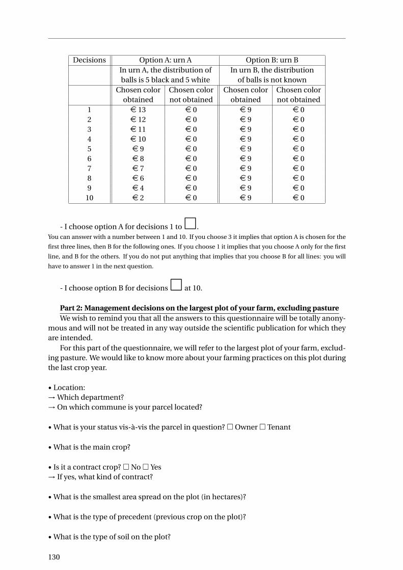
Decisions Option A: urn A Option B: urn BIn urn A, the distribution of In urn B, the distributionballs is 5 black and 5 white of balls is not known
Chosen color Chosen color Chosen color Chosen colorobtained not obtained obtained not obtained
1 e 13 e 0 e 9 e 02 e 12 e 0 e 9 e 03 e 11 e 0 e 9 e 04 e 10 e 0 e 9 e 05 e 9 e 0 e 9 e 06 e 8 e 0 e 9 e 07 e 7 e 0 e 9 e 08 e 6 e 0 e 9 e 09 e 4 e 0 e 9 e 0
10 e 2 e 0 e 9 e 0
- I choose option A for decisions 1 to�.You can answer with a number between 1 and 10. If you choose 3 it implies that option A is chosen for the
first three lines, then B for the following ones. If you choose 1 it implies that you choose A only for the first
line, and B for the others. If you do not put anything that implies that you choose B for all lines: you will
have to answer 1 in the next question.
- I choose option B for decisions� at 10.
Part 2: Management decisions on the largest plot of your farm, excluding pastureWe wish to remind you that all the answers to this questionnaire will be totally anony-
mous and will not be treated in any way outside the scientific publication for which theyare intended.
For this part of the questionnaire, we will refer to the largest plot of your farm, exclud-ing pasture. We would like to know more about your farming practices on this plot duringthe last crop year.
• Location:→ Which department?→ On which commune is your parcel located?
• What is your status vis-à-vis the parcel in question? � Owner � Tenant
• What is the main crop?
• Is it a contract crop? � No � Yes→ If yes, what kind of contract?
• What is the smallest area spread on the plot (in hectares)?
• What is the type of precedent (previous crop on the plot)?
• What is the type of soil on the plot?
130

• What was your target for early returns (in qt/ha)?
• What were your real yields after harvest (in qt/ha)?
→ If objective and real returns have been different, please explain why:
• Have you applied one (or more) organic nitrogen fertilizer on this plot? � No � Yes→ If yes, how much (in kg/ha)?→How was the amount of nitrogen contained in this (these) intake (s) taken into account?� Analysis � Reference table � It was not taken into account→ Does mineral nitrogen fertilizer advice take into account this quantity? � No � Yes
• Have you buried the fertilizer? � No � Yes
In terms of mineral nitrogen fertilization:
• Please indicate the amount of mineral nitrogen recommended by your nitrogen advi-sory agency on this plot (in kgN/ha)?
• Was there any advice on the first nitrogen intake? � No � Yes→ If yes, how much (in kg/ha)?
• Have you been advised to split contributions? � No � Yes→ If yes, how much ?
• Did you split the contributions? � No � Yes→ If yes, how much ?
Regulatory Doses:• Is there a maximum that you should not exceed on this parcel? � No � Yes.→ If yes, how much (in kg/ha)?
• Is there a type of spreading that you must follow? � No � Yes→ If yes, which one?→ If yes, what is this regulatory constraint related to? � Vulnerable area � MAE � Other
Actual decisions of mineral nitrogen fertilization:• How much did you actually apply to this parcel in total (in kgN/ha)?
• And at the first intake (in kgN/ha)?→ Explain the reasons for your choice:
• What is the share of synthetic nitrogen fertilizer costs in your total expenses for this par-cel (in %)?
Some additional questions on your farm:
• How much PAC assistance do you receive in total (ine/year)?
131

→ Of this total amount, which amount corresponds to specific environmental aids andthe reduction of the chemical spreading do you perceive (MAE or other) (ine/year)?
• Have you signed this year a voluntary agricultural yield insurance? � No � Yes
• What is the total area of your farm (in hectares)?
• Are you part of an operator’s union? � No � Yes→ If yes which?
Part 3: Socio-economic characteristicsAnswers to these questions are essential to properly analyze your decisions. We re-
mind you that your answers will be treated anonymously.
• What is your age in years ?
• Sex: � Man � Woman
• Marital status: � Single � Married � Pacsé
• Level of studies :� Without diploma � Brevet � Bac� Baccalaureate + (specify the number of years of study after baccalaureate:....)
• Number of people in the household: � 1 � 2 � 3 � 4 and moreAmong them, how much children ?
• In what interval are the total monthly incomes of your household (net of taxes)?� <e1000/net/month � from 1000 toe1500/net/month� from 1500 toe2000/net/month � from 2000 toe2500/net/month� from 2500 toe3000/net/month � >e3000/net/month
• Here you can express your opinion on synthetic nitrogen fertilizers and policies to reg-ulate their use:
• Here you can give us your opinion on the survey (strengths, possible difficulties encoun-tered, etc.):
Email address for the return of the results:
THANKS FOR YOUR HELPWE WILL TRANSMIT YOUR INDIVIDUAL RESULTS WHEN THEY WILL BE PROCESSED
132

Chapter 5
Concluding comments
Contents5.1 Uncertainty, irreversibility and information at the core of farmers’ re-
luctance to adopt . . . . . . . . . . . . . . . . . . . . . . . . . . . . . . . . . 134
5.2 Volatility in grass yields can prevent us from taking benefits from thepotential of grasslands carbon sink . . . . . . . . . . . . . . . . . . . . . . 135
5.3 Not only risk but ambiguity aversion impact N2O emissions mitigationrelated to nitrogenous fertilization practices . . . . . . . . . . . . . . . . . 136
133

CHAPTER 5. CONCLUDING COMMENTS
This thesis focuses on the role of uncertainty as a barrier to adoption of mitigationpractices in the agricultural sector. The literature explicitly shows that most of these prac-tices may be of high technical quality and source of benefits for farmers. However, thesemitigation practices can wear uncertainty and farmers can have misperceptions of thepotential profits. This uncertainty prevents them from adopting if it negatively impactsthe farmers profits evaluation or the utility they expect from their farming activities. Iden-tifying the drivers of uncertainty’s effect on adoption and quantifying it about some givenpractices is a first step that we did in this thesis. Our findings contribute to a better un-derstanding of individuals’ adoption choices drivers and a better identification of the en-vironmental and agricultural policies targets and design.
The effect of uncertainty on agents’ microeconomic choices is often introduced throughseparated channels in the litterature. We adopted a strategy of merging these diverse con-cepts, that can be associated in order to produce improvements in the comprehensionof farmers’ adoption decisions. This approach leads us to do three main studies whichpartly answer the main question in an eclectic way.
5.1 Uncertainty, irreversibility and information at the coreof farmers’ reluctance to adopt
We show that in a situation of uncertainty, typically with mitigation sufficiently disrup-tive or innovative in the usual farm management, uncertainty generates three different(possibly coexistent) hidden costs, and bad information can limit diffusion from earlystages. We merge the diversification processes toward environmental friendly practiceswith a real option approach embedded with information through beliefs updatings. Thisframework allows us to take into account specific (physical) constraints of agriculturalproductions: the maximum land available constraint and the portfolio of land alloca-tion in different activities. Irreversibility is introduced progressively. We introduce riskpreferences and risk premia, while it is rarely used in real option theory. More precisely,we show that irreversibility makes dynamic choices non-separable, and negative signalsare potentially lowering the willingness to adopt through the worse forecasts farmers canmake. Under risk neutrality, a quasi-option value arises with irreversibility, which is a firsthidden cost. Under risk aversion, risk premia are added as a second hidden cost at eachperiod, that depends on individual preferences toward risk. Thirdly, with irreversibilityand risk aversion, an irreversibility premium composed by risk premia plus quasi-optionvalue that coexist, weights the profits evaluation from the first period and act like a hid-den cost. Irreversibility and the choice dynamic create an asymmetry between bad andgood signals’ impact on profits evaluation. Bad signals at early stages can "nip diffusionin the bud". While most of current agricultural public incentives target diversification offarming practices toward mitigation practices, we claim that policy makers should takeinto account flexibility or irreversibility of these practices in their design, and socializethe costs associated to uncertainty in order to unlock diffusion of practices with negativeabatement costs.
Different extensions can be done later on. First, we want to append a farm internalsignal production into the information function. This extension would allow us to showarbitrage than can be made by farmers between adopting and taking benefit from theirown information production about the potential good new practice, or not adopting and
134

CHAPTER 5. CONCLUDING COMMENTS
observe external signals. The role of risk aversion and irreversibility may be of a greatimportance in this decision process, and may allow us to make a clear distinction in thedriver of being a early or a lately adopter, with all the subsequent implications in the dif-fusion process. Secondly, the cost-efficiency of our political propositions has to be as-sessed. We claim that given the fact that some mitigation practices wear negative abate-ment costs, issues can arise from other perspectives than a classic matter of compensa-tion from losses, and alternative policies can suffice to unlock adoptions if they reduceuncertainty and provide knowledge about practices quality to farmers. In this purpose,targeting one region where conditions seem reunited for high level of adoption and suc-cess of farm transformation, and spread good information around, can be a solution thatlower the cost for the policy maker and achieve better results than current measures (flatinclusive subsidies). The cost-efficiency of providing higher but decreasing and tempo-rary subsidies for mitigations wearing irreversibility, must be checked too.
5.2 Volatility in grass yields can prevent us from taking ben-efits from the potential of grasslands carbon sink
Increasing the share of grasslands into rotations of farmers-breeders can induce poten-tial huge benefits for them. But volatility of herb yields, their high level of interactionwith meteorological conditions and the lower number of technical levers associated toherb management with respect to this meteorological dependency compared to annualforage crops is a well-known issue in the topic of herb systems promotion. We develop ashort static-dynamic model of stochastic land allocation and different measures of uncer-tainty, related to yields shocks and to yields volatility. We test empirically our assumptionsthrough a classic land-use econometric panel model estimation with fixed-effects, andran several regressions in order to check the robustness of results with respect to diverseassumptions : naive regressions, time dummies, control variables, and finally instrumen-tation method in order to tackle endogeneity. We show that Natural and old-seeded grass-lands’ yields shocks impact positively land-use ratio of each type of grasslands in the for-age mix, as well as the alternative annual crop (ensilage maize) whose yields shocks im-pact Artificial grasslands like in a risk-hedging diversification strategy. This result showshow yields fluctuations lead to arbitrage between grasslands and strongly impact theiruse. We show that the temporary grasslands ratio in the forage mix is negatively impactedby OU measures and positively by MA measures, while the Artificial grasslands ratio in theforage mix is positively impacted by OU measures and negatively by MA measures, whilethe results are not clear-cut for Natural and old-seeded grasslands. We interpret this dif-ference by the fact that OU measures can be attributed to long-term volatility forecastswhile MA measures can rather be associated to short-term volatility forecasts. Given theestimated marginal impact of uncertainty, it is a crucial component of farmers-breederschoices, and has a non-negligible effect on the possibility of further development of grass-lands in rotations. This impact must be hedged by the regulator in order to reach the po-litical goal of grasslands promotion.
A tension can arise between policies aiming at conserving the carbon stocks of perma-nent grasslands by forbidding their destruction, and the potential of carbon sink relatedto adopting new grasslands for the current livestock. Uncertainty may induce that thisenvironmental policy has a perverse effect, leading farmers not to lock into grasslands,whose yields are too uncertain compared to annual intensive crops, if they increase too
135

CHAPTER 5. CONCLUDING COMMENTS
much the duration of non-permanent grasslands. This conclusion leads to a clear propo-sition for an extension: in order to check this assumption, it would be interesting to makea complete assessment of sustainable carbon storage in soil in grasslands over time andsequestration potential across years, together with integrating abatement costs, uncer-tainty and irreversibility. Making parameters associated to regulation move (especiallyconsidering grasslands destruction and subsidies design) can be a good simulation of theprocesses involved and the impact on GHG net emissions. Simulating the impact of pro-viding centralized forage stocks in case of negative shocks, other insurance strategies, orthe impact of the development of new levers aiming at improving herb production stabil-ity can be of interest too.
5.3 Not only risk but ambiguity aversion impact N2O emis-sions mitigation related to nitrogenous fertilization prac-tices
Individual’s preferences in a situation of uncertainty are known to impact practices asso-ciated to intensive margins. Nitrogen fertilization is a good example of that. Meanwhile,farmers together with cooperatives agents try to find margins in fertilization practicesthat can allow to achieve yields goals while limiting N2O emissions, and policy makersencourage farmers to reduce nitrogen fertilization by compensating the average poten-tial loss due to nitrogen limitation. Nitrogen fertilizers have an effect on the stochasticityassociated to yields, and farmers already know well the probabilistic distribution of yieldsrelated to input uses. Then, depending on the risk-decreasing or increasing nature of thefertilizer and farmers’ preferences, nitrogen will be more or less applied, so that recip-rocally emissions abatement will be enhanced or limited. Ambiguity preferences wouldcatch a deeper level of uncertainty and adopting new practices of fertilizer application canfall in this particular situation, if you multiply the number of possible outcomes embed-ded with different states-of-the-nature. We test experimentally if there exist significantimpacts of risk and ambiguity preferences on fertilization practices: total fertilization andfertilization at the first splitting. We used a MPL approach and a questionnaire for farm-ing practices and socio-economics variables on a sample of 45 French Farmers. Some ofour results are close to previous results in the literature, and we find that our sample isslightly statistically different from French farmers at the national level for some charac-teristics. We find that risk averse farmers apply less nitrogen fertilizer than risk neutralone in total. However, we also find that the more farmers are ambiguity averse, the morethey apply nitrogen fertilizer at the first splitting.
We interpret the first result as a consequence of the possible risk-increasing nature offertilizer with respect to the meteorological conditions during the last agricultural cam-paign. The second result would be related to the deep uncertainty which is associated tothe splitting practice, because it relies on a difficulty to forecast future natural conditionsthat will allow or not sidedressing. Because risk aversion decreases whole fertilization itcan be interpreted as a abatement co-benefit, while ambiguity aversion can be consid-ered as a hidden abatement costs because splitting practice is a well-known approach todecrease N2O emissions from fertilization. However, we have not enough observations tocontrol for crucial variables, like the cultivated crop on the parcel, the precedent crop andsoil type. We can’t either make parallel analysis with key variables, like insurance coverageor sales contracts types, or other interactions and control variables. Other extensions are
136

CHAPTER 5. CONCLUDING COMMENTS
possible and can be done in future works: controlling for discounting behaviors, doing acontextualized experiment, testing for prospects and probabilities transformation are allextensions that we are currently considering. Developing a theoretical behavioral modelthat explains the ambiguity aversion effect we found experimentally, as well as finding in-novative policies that can have an impact on ambiguity-related behaviors will be needed.
137

CHAPTER 5. CONCLUDING COMMENTS
138

Chapter 6
Summary of the thesis (French)
139

L’incertitude en tant que frein à l’adoption demesures d’atténuation en agriculture
Camille TEVENART
16 octobre 2019

CHAPTER 6. SUMMARY OF THE THESIS (FRENCH)
Cette thèse porte sur le rôle de l’incertitude en tant que frein à l’adoption de mesuresd’atténuation par les agriculteurs. Le changement climatique est un enjeu de poids faceauquel de nombreuses politiques publiques ont été mises en place dans les différentssecteurs de l’économie, notamment en France. Son atténuation est l’un des principauxchallenges auquel les producteurs de biens et services font face, et l’agriculture n’est pasen reste compte tenu du niveau de ses émissions et de son potentiel de réduction d’émis-sions nettes. Plusieurs mécanismes incitatifs ont été mis en place afin d’encourager lesagriculteurs à mener individuellement des actions d’atténuation de leurs émissions, viales changements d’un certain nombre de pratiques de production agricoles. La théorieéconomique classique visant à internaliser le coût du changement climatique dans lesproductions agricoles conduit à mesurer le coût d’abattement de pratiques dites de référen-ces et d’établir le niveau de taxe optimal permettant d’atteindre des objectifs de réductionfixés par les pouvoirs publics. Dans le cas de taxes "négatives" (subvention), il s’agit derémunérer les agriculteurs pour des actions de réduction des émissions en compensantl’ensemble des coûts supportés par ceux-ci s’ils modifient leurs pratiques par rapport auxpratiques conventionnelles. C’est ainsi que fonctionne la quasi-totalité de la politiqued’atténuation du changement climatique en agriculture en France, notamment du faitde la non-participa-tion du secteur au marché EU-ETS et de la difficulté de mettre enplace un système de régulation stricte des pratiques qui augmenterait les charges opéra-tionnelles des agriculteurs, dont un nombre important supporte déjà des charges élevéeset une concurrence accrue sur les marchés internationaux : en effet, le développementrural et agricole est un enjeu collatéral fort des politiques agro-environnementales.
Dans cette perspective, un certain nombre de questions se sont posées récemmentà propos de ces politiques incitatives. Premièrement, leur efficacité est remise en caused’un point de vue ex post. En effet, si les résultats en terme d’adoption concrète de nou-velles pratiques dans la constellation d’exploitations agricoles sont difficilement mesura-bles, les émissions totales du secteur agricole sont en revanche celles qui diminuent lemoins tous secteurs confondus, rendant les objectifs de réduction des émissions de plusen plus éloignés. Par ailleurs, le secteur peine souvent à se transformer, comme le mon-trent l’échec du programme Ecophyto concernant l’utilisation de produits phytosani-taires, ou autre exemple, le lent taux de progression de l’agriculture biologique dans l’ensem-ble du secteur. L’agriculture semble être le secteur économique national le plus inerteen terme de changements de pratiques liés à l’atténuation. Deuxièmement, l’estimationdes coûts d’abattement associés aux principales pratiques d’atténuation a montré qu’unnombre significatif de pratiques présentent des coûts négatifs, autrement dit des béné-fices nets pour les agriculteurs qui les adopteraient sur leur exploitation. Ce résultat n’estpas unique, en agriculture comme dans d’autres secteurs, en France comme ailleurs.La présence de bénéfices nets potentiels à la réduction des émissions pose cependantla question des freins qui peuvent limiter la diffusion de pratiques d’atténuation. Cesfreins économiques, qui cohabitent avec des freins sociologiques et comportementaux,agissent comme des coûts "cachés" qui sont non seulement absents du calcul des coûtsd’abattement car non pris en compte pour l’instant dans les coûts mesurables, mais surtoutmènent à des défaillances potentielles des politiques publiques qui ne les intègrent pasdans leur design. Les subventions étant censées permettre de corriger des défaillances demarchés, se retrouvent inefficaces sans cette correction, ce qui limite l’atteinte des objec-tifs politiques environnementaux. Différents coûts "cachés" sont évoqués dans la littéra-ture portant sur l’adoption de nouvelles pratiques en agriculture, et parmi eux, l’un desprincipaux est l’incertitude. Cette thèse se propose d’explorer ce sujet, en montrant com-
2

CHAPTER 6. SUMMARY OF THE THESIS (FRENCH)
ment l’incertitude peut, via différents canaux, limiter l’adoption de pratiques d’atténuationpar les agriculteurs. Les méthodologies adoptées sont éclectiques : passant de la modéli-sation théorique, à l’économétrie, à l’expérimentation, nous nous proposons d’aborder laquestion de recherche sous différents angles, théoriques comme empiriques.
Le premier chapitre (1) constitue un état de l’art stylisé de la littérature portant sur lerôle de l’incertitude sur les choix de changement de production des agriculteurs. Aprèsavoir caractérisé les principales pratiques d’atténuation du changement climatique enagriculture de manière générale, nous passons en revue les principaux canaux par lesquelsl’incertitude peut engendrer des freins aux changements de pratique agricole. Ces canauxsont ceux que nous empruntons au cours de la thèse, selon les besoins du sujet d’étude dechaque chapitre. Nous les présentons tels qu’ils sont presque toujours présentés dans lalittérature, c’est-à-dire séparés et faisant l’objet de conclusions parfois très différentes. Ladistinction Knightienne entre risque et incertitude (que nous appelons ici, incertitude ausens stricte) a beaucoup compté dans cette dichotomie historique. Le risque et les com-portements face au risque sont les premiers drivers que nous présentons : présents dansla littérature d’économie agricole depuis très longtemps, ils constituent une explicationfondamentale de nombreux comportements de production des agriculteurs. Les agricul-teurs ayant de l’aversion pour le risque cherchent à se couvrir contre celui-ci ou à éviterde prendre de nouveaux risques qui ne seraient pas couverts par suffisamment de profitsupplémentaire ou par un mécanisme de couverture du risque. Ces comportements, quisont fortement liés aux caractéristiques des pratiques en terme de prise de risque, peu-vent constituer un coût caché qui, s’il n’est pas intégré dans les incitations économiques,empêche les exploitants d’adopter de nouvelles pratiques. L’abondante littérature surcette question montre que le sujet mérite d’être appliqué aux pratiques d’atténuation,afin d’améliorer la conception des subventions et autres politiques incitatives. Le risquecorrespond cependant à des cas où les profits sont incertains mais probabilisables ob-jectivement, ce qui correspond à un niveau de connaissance élevé des pratiques asso-ciées. C’est le contraire dans le cas de l’incertitude au sens stricte (suivant la distinctionde Knight) qui est associée à des cas où la pratique d’atténuation est suffisamment inno-vante pour que les agriculteurs n’aient pas assez de recul et de connaissance sur les prof-its associés. Il s’agit du deuxième canal que nous présentons. L’incertitude est en généralmodélisée dans cette situation via des croyances subjectives que les agents peuvent for-mer sur les distributions de profits des nouvelles pratiques. Ce second courant de littéra-ture, moins abondant en agriculture, met l’accent sur la dépendance des producteurs àleurs croyances initiales mais également à ce qu’ils peuvent observer de la vraie valeur desprofits engendrés par l’innovation, donc, à l’information reçue par l’exploitant. Générale-ment étudiée dans le prisme de la théorie des options réelles, elle donne un rôle profondà l’irréversibilité de l’adoption d’innovation, dans ce qu’elle conduit à un regret poten-tiel si celle-ci se révèle moins profitable que la pratique conventionnelle. L’agriculteurne sachant pas initialement la distribution réelle des profits de la nouvelle pratique, ilpeut être poussé à recueillir suffisamment d’information afin de déterminer son choixoptimal. Contrairement au risque, où l’accent est donné à la forme de la distributionconnue des profits et aux préférences individuelles pour certaines formes de distribu-tions (plus ou moins dispersées notamment), l’incertitude au sens stricte met l’accentsur les croyances et les anticipations sur les profits espérés, ainsi que leur mise à jourau cours du temps et leur comparaison face au statu quo. Nous introduisons le fait quesi la distinction knightienne est généralement cruciale car chaque courant de pensée sedéveloppe sur des hypothèses, fonctionne sur des méthodologies, et mène à des conclu-
3

CHAPTER 6. SUMMARY OF THE THESIS (FRENCH)
sions et préconisation bien différentes, elle peut cependant être allégée dans l’étude decertaines pratiques d’atténuation selon les besoins méthodologiques du chercheur. Ledernier canal par lequel l’incertitude peut constituer un frein à l’adoption de nouvellepratique est l’ambiguïté. Elle correspond à une situation dans laquelle un "risque derisque" pèse sur les profits des pratiques agricoles, c’est-à-dire, que les probabilités as-sociées à la distribution objective des profits sont elles-mêmes incertaines. Des pratiquesrelativement connues des agriculteurs, associées à des connaissances suffisantes sur lerisque qu’elles revêtent, peuvent devenir source d’une incertitude plus profonde si desmodifications qu’on y apporte entraînent un doute sur la distribution de profits qui peu-vent en être générés. Imaginons qu’une pratique courante et connue soit remise en causepar un conseiller agricole afin de modifier le mode d’administration d’un intrant déjà util-isé ou le mode de gestion d’une culture déjà cultivée sur la ferme, dans le but de tirerparti d’un gain d’efficacité à la marge : ce changement de pratique peut conduire simul-tanément à des économies et à une réduction des émissions de gaz à effet-de-serre. Lesprocessus biophysiques inhérents à la production agricole, qui sont une interconnexioncomplexe de phénomènes naturels stochastiques dans lesquels l’agriculteurs doit nor-malement apporter des leviers agronomiques, mènent à une remise en cause de ce quel’agriculteur croit être la distribution correcte de ses profits. Dans ce cas, plusieurs distri-butions peuvent cohabiter dans l’esprit de l’exploitant, une situation qu’il peut déprécieret vis-à-vis de laquelle il peut chercher à se prémunir et se couvrir. La littérature est as-sez récente sur le sujet, et particulièrement limitée dans le cas de l’adoption de pratiquesd’atténuation en agriculture. Nous introduisons l’intérêt que cette approche revêt, en tantque troisième canal. Enfin, nous présentons les contributions de chaque chapitre.
Le second chapitre (2) constitue une approche théorique de la question de recherche,dont la principale caractéristique est d’introduire l’irréversibilité de l’adoption d’une nou-velle pratique au cœur de la préoccupation de l’agriculteur, du fait de l’incertitude, con-jointement aux préférences face au risque. Ici, les probabilités associées aux profits in-certains sont considérées comme des croyances subjectives bayésiennes, mais les profitssont cependant susceptibles d’être considérés comme risqués par l’agriculteur. Cela im-plique la conjonction d’un phénomène de type option réelle induisant une prime d’irréver-sibilité et de l’apparition de primes de risque, ainsi que la possibilité d’externalités infor-mationnelles liées à la mise-à-jour bayésienne des croyances. La structure du modèlenous permet d’extraire les coûts "cachés" liés à la valeur d’option et au risque de manièreséparée, mais pouvant cohabiter ou être liés selon les caractéristiques de l’exploitant et dela nouvelle pratique. L’externalité informationnelle notamment, n’est supposée possibleque dans le cas d’adoption partielle que nous expliquons grâce à l’aversion au risque. Ilest ainsi possible que l’effet de l’irréversibilité ne limite pas l’adoption sans aversion aurisque, mais que ce soit le cas avec aversion au risque si cela conduit à une externalité in-formationnelle générée par les premiers adoptants. Nous illustrons ces résultats dans unesimulation avec calibration sur données réelles dans le cas de l’adoption de miscanthus,une culture servant à la production de bio-fuel, qui est une culture pérenne aux profitsincertains. Nous présentons une situation originale permettant de mesurer les différentscoûts et l’impact sur le niveau d’adoption, mais aussi d’illustrer ce phénomène spécifiqued’externalité informationnelle en cas d’aversion au risque.
Le troisième chapitre (3) s’attache à mesurer empiriquement l’impact de l’incertitudesur l’allocation de terres fourragères aux prairies en France. En effet, l’adoption de plus deprairies dans les rotations (pour fauche ou pâturage) constitue une pratique d’atténuation
4
CHAPTER 6. SUMMARY OF THE THESIS (FRENCH)
à très forts potentiels et co-bénéfices environnementaux, et à coût d’abattement négatif.Nous partons de l’hypothèse que l’incertitude sur les rendements herbagers peut con-stituer un frein à leur plus ample adoption en ce qu’elle peut réduire la valeur implicitede l’usage "prairies" des terres agricoles à destination fourragère, vis-à-vis de cultures an-nuelles étant moins complexes et pour lesquelles l’agriculteur a plus de leviers de sta-bilisation tel que le maïs ensilage. Devoir verrouiller une partie de ses terres dans desprairies, même temporaires, peut ainsi être difficile du fait de la volatilité des rende-ments herbagers. Nous nous proposons de mesurer l’impact de l’incertitude sur les ren-dements grâce à un modèle économétrique d’usage des terres en panel sur les départe-ments métropolitains, dans le cas des trois principaux types de prairies fourragères : lesprairies temporaires et artificielles (non permanentes) et les prairies naturelles ou seméesdepuis plus de 5 ans (permanentes). Un avantage de cette distinction dans les donnéeset que chaque type de prairie n’est pas de la même nature et ne revêt pas le même niveaud’irréversibilité. L’incertitude est mesurée via différents indicateurs que nous avons voulucomplémentaires. Des problèmes d’endogénéité nous conduisent à employer la méth-ode instrumentale en utilisant des données météorologiques agrégées, et à chercher pardifférents moyens les résultats les plus robustes. Ceux-ci montrent que l’incertitude im-pacte différemment les parts relatives des divers types de prairies fourragères dans les ro-tations départementales, de manière souvent symétrique. L’incertitude impacte surtoutl’allocation de terres aux prairies non-permanentes, parfois positivement et parfois néga-tivement. Certains effets de complémentarité entre les diverses options de fourrages encas de chocs sont aussi visibles. L’ensemble de ces phénomènes conduit à la conclu-sion que l’incertitude joue un rôle particulièrement fort dans la propension à adopter desprairies dans les rotations, rôle qui doit être pris en compte dans les politiques publiquesdans le but d’inciter correctement à leur déploiement. Par exemple, l’allocation aux prai-ries temporaires, qui sont destinées à devenir des prairies permanentes protégées si ellesne sont pas déplacées ou détruites au bout de cinq ans (et doivent donc stocker du car-bone), est particulièrement impactée négativement par notre mesure de volatilité de longterme : plus la volatilité est intense et plus nous mesurons une désallocation dans ce typede prairie, ce qui pourrait remettre en cause la production de nouvelles prairies perma-nentes et donc le puit de carbone associé, à cause d’un effet d’irréversibilité.
Dans un quatrième chapitre (4) nous abordons le cas de la réduction de la fertilisationazotée, mesure d’atténuation fondamentale, qui concerne une pratique déjà bien con-nue des agriculteurs. La modulation des apports en fertilisants azotés peut conduire àdes gains d’efficacité et une réduction des émissions de N2O. Portés par de précédentesrecherches sur le rôle des préférences face au risque sur le niveau de fertilisation, noustentons d’apporter une confirmation ou non des précédents résultats sur le sujet maisaussi d’étendre l’étude aux préférences face à l’ambiguïté. Nous utilisons pour ce fairedes méthodes expérimentales de mesure des préférences suffisamment validées dans lalittérature et les combinons avec des questions économiques et agronomiques sur les dé-cisions de fertilisation. L’étude a été réalisée sur un échantillon de 45 agriculteurs. Dif-férentes techniques économétriques sont appliquées afin de prendre en compte le plande sondage complexe et extraire du mieux possible des résultats significatifs. Il est mon-tré que les agriculteurs ayant de l’aversion pour le risque fertilisent moins sur l’ensemblede la campagne agricole que les agriculteurs neutres au risque. Cela implique que les fer-tilisants azotés doivent être perçus comme impactant positivement le niveau de risque,et dans ce cas l’aversion au risque n’est pas un coût "caché" à la réduction de la fertili-sation azotée. Le niveau d’aversion à l’ambiguïté n’impacte pas le niveau de fertilisation
5

CHAPTER 6. SUMMARY OF THE THESIS (FRENCH)
totale. En revanche, nous montrons qu’il conduit à mettre significativement plus de fer-tilisants azotés au premier apport en cas de "splitting", une technique visant à ajuster lesapports aux besoins des plantes en séparant les applications, ce qui fait partie des pra-tiques d’atténuation possibles liées à la fertilisation azotée. Ainsi, mettre plus de fertil-isants pourrait conduire à émettre plus de N2O et donc réduire l’intérêt environnemen-tal d’une telle pratique. Nous interprétons ce résultat comme une conséquence directede l’incertitude profonde qui règne en cas de "splitting" sur les possibilités d’applicationpostérieure et la réponse des cultures à ce type de procédé. Ce résultat montre que lespratiques d’atténuation, selon leurs caractéristiques spécifiques en terme d’interactionsentre les conditions pédoclimatiques et les décisions de production, peuvent se révélerambigües, ce qui impliquerait un coût "caché" de type nouveau à prendre en compte.
Le dernier chapitre (5) conclut la thèse. Après avoir replacé le travail dans la questionde recherche globale, nous résumons les contributions de chaque chapitre en ouvrant lesperspectives futures que nos résultats impliquent. Nous rappelons l’intérêt de ce travail: mieux comprendre les comportements des agriculteurs, démontrer que l’incertitudepeut mener à des freins à l’adoption de pratiques d’atténuation via différents vecteurs, etqu’elle doit impérativement être prise en compte par les politiques publiques afin d’attein-dre les objectifs environnementaux que les pouvoirs publics ont fixé.
6