Uncertainty Analysis

2141-375 Measurement and Instrumentation

Measurement Error

Mea

sure

d va

lue,

x

x

'xTrue data

Bias error

Precision error in xi

Measurement number

Uncertainty defines an interval about the measured v alue within which we suspect the true value must fallWe call the process of identifying and quantifying e rrors as uncertainty analysis.

Design-Stage Uncertainty Analysis

Design-stage uncertainty analysis refers to an initia l analysis performed prior to the measurement

Useful for selecting instruments, measurement techniq ues and to estimate the minimum uncertainty that would resu lt from the measurement .

Design-Stage Uncertainty Analysis

%)( 220 Puuu cd += RSS method for combining error

Design-state uncertainty22

0 cd uuu +=

Design-state uncertainty

Interpolation error

0uInstrument error

cu

Zero-Order Uncertainty (Interpolation Error)Even when all error are zero, the value of the measurand must be

affected by the ability to resolve the information pro vided by the instrument. This is called zero-order uncertainty. At z ero-order, we assume that the variation expected in the measurand will be less than that caused by the instrument resolution. And that al l other aspects of the measurement are perfectly controlled (ideal condi tions)

(95%) resolution 2/10 ±=u

Design-Stage Uncertainty Analysis

Instrument Uncertainty, uc

This information is available from the manufacturer ’s catalog

x

y

resolution

yo

uncertainty1/2 resolution

Design-Stage Uncertainty Analysis

0-1000 cm H2O±15 V dc0-5 V0-50oC nominal at 25oC

±0.5%FSOLess than ±0.15%FSO±0.25%of reading0.02%/oC of reading from 25oC0.02%/oC FSO from 25oC

OperationInput rangeExcitationOutput rangeTemperature rangePerformanceLinearity error eL

Hysteresis error eh

Sensitivity error eS

Thermal sensitivity error eST

Thermal zero drift eZT

Specifications: Typical Pressure Transducer

The root of sum square approach:

223

22

21 nrss eeeee L+++= (95%)

Example: Consider the force measuring instrument described by the catalog data that follows. Provide an estimate of the uncertainty attributable to this instrument and the instrument design state uncertainty.

Known: Instrument specifications

Solution:

Assume: Values representation of instrument 95% pro bability

Design-Stage Uncertainty Analysis

Force measuring instrumentResolution: 0.25 N Range: 0 - 100 NLinearity: within 0.20 N over range Repeatability: within 0.30 N over range

Design-state uncertainty22

0 cd uuu +=

Design-state uncertainty

0u cu

½ Resolution = 0.125 N N 36.03.02.0 2222 ±=+±=+ rl ee

N 38.036.0125.0 22 ±=+±=du

Example: A voltmeter is to be used to measure the output from a pressure transducer that outputs an electrical signal. The nominal pressure expected will be ~3 psi (3 lb/in2). Estimate the design-state uncertainty in this combination. The following information is available:

Known: Instrument specifications

Solution:

Assume: Values representation of instrument 95% pro bability

Design-Stage Uncertainty Analysis

VoltmeterResolution: 10 µV Accuracy: within 0.001% of reading

TransducerRange: ±5 psiSensitivity: 1 V/psiInput power: 10 Vdc ± 1%Output: ±5 VLinearity: within 2.5 mV/psi over rangeRepeatability: within 2 mV/psi over rangeResolution: negligible

Design-Stage Uncertainty Analysis

Design-state uncertainty

( ) ( )22

PdEdd uuu +=

Design-state uncertainty

Design-state uncertainty

( ) ( ) ( )220 EcEEd uuu +=

Design-state uncertainty Design-state uncertainty

( ) ( ) ( )220 PcPPd uuu +=

Design-state uncertainty

Error Propagation

Computation of the overall uncertainty for a measur ement system consisting of a chain of components or several instruments

Let R is a known function of the n independent variables xi1, xi2 , xi3, …, xiL

),,,( 21 LxxxfR K=

L is the number of independent variables. Each variab le contains some uncertainty ( ux1, ux2, ux3,…, uxL) that will affect the result R.

%)( ' PuRR R±=

Application of Taylor’s expansion gives, (neglect t he higher order term)

xLL

xx

LxLLxx

ux

fu

x

fu

x

f

xxxfuxuxuxfRR

∂∂

++∂∂

+∂∂

+≈±±±=∆±

...

),...,,(),...,,(

22

11

212211

The best estimate value, R’

Where ),...,,( 21 LxxxfR =

Error Propagation

( ) %)( 1

2

22

22

2

11

Pu

ux

fu

x

fu

x

fu

L

ixii

xLL

xxR

∑=

±=

∂∂

++

∂∂

+

∂∂

±=

θ

K

The combination of uncertainty of all variables (pr obable estimate of uR)

Where θθθθi is the sensitivity index relate to the uncertainty of xi

ii x

f

∂∂

=θ

Example: For a displacement transducer having a calibration curve y = KE, estimate the uncertainty in displacement y for E = 5.00 V, if K = 10.10 mm/V with uk = ±0.10 mm/V and uE = ±0.01 V at 95% confidence

Solution: Find uy

Error Propagation

Known: y = KEE = 5.00 V uE = 0.01 VK = 10.10 mm/V uk = 0.10 mm/V

( ) ( )22KKEEy uuu θθ +±=

KE

yE =

∂∂

=θ EK

yK =

∂∂

=θ

uE = 0.01 V uK = 0.10 mm/V

yy uKEuyy ±=±='

( ) ( )

( ) ( ) mm 51.0mm/V 10.0V 5V 01.0mm/V 10.10 22

22

±=×+×±=

+±= KEy EuKuu

Sequential Perturbation

A numerical approach can also be used to estimated the propagation of uncertainty. This refers to as sequential perturba tion. This method is straightforward and uses the finite difference to a pproximate the derivatives (sensitivity index)

1) Calculate the average result from the independen t variables

),...,,( 21 LxxxfR =

2) Increase the independent variables by their resp ect uncertainties and recalculate the result based on each of these n ew values. Call these values +

iR

),...,,(

),...,,(

),,...,,(

21

2212

2111

LLL

L

L

uxxxfR

xuxxfR

xxuxfR

+=

+=

+=

+

+

+

3) Decrease the independent variables by their resp ect uncertainties and recalculate the result based on each of these n ew values. Call these values −

iR

Sequential Perturbation

4) Calculate the difference for each element

RRR

RRR

ii

ii

−=

−=−−

++

δ

δ

5) Finally, evaluate the approximation of the uncer tainty contribution from each variables

ii

ii

i uRR

R θδδ

δ ≈+

=−+

2

The uncertainty in the result

( )2/1

1

2

±= ∑

=

L

iiR Ru δ

),...,,(

),...,,(

),,...,,(

21

2212

2111

LLL

L

L

uxxxfR

xuxxfR

xxuxfR

−=

−=

−=

−

−

−

Example: For a displacement transducer having a calibration curve y = KE, estimate the uncertainty in displacement y for E = 5.00 V, if K = 10.10 mm/V with uk = ±0.10 mm/V and uE = ±0.01 V at 95% confidence

Solution: Find uy

Error Propagation

Known: y = KEE = 5.00 V uE = 0.01 VK = 10.10 mm/V uk = 0.10 mm/V

i u i x i +u i x i -u i R i+ R i

- δδδδ R i+ δδδδ R i

- δδδδ R i

1 E 5 0.01 5.01 4.99 50.60 50.40 0.10 -0.10 0.10

2 K 10.1 0.1 10.20 10.00 51.00 50.00 0.50 -0.50 0.50

x i

( ) ( )22KEy RRu δδ +±=

yy uKEuyy ±=±='

( )( ) mm 50.50510.10 === KEy

Steps in measurement process1) Calibration2) Data-acquisition3) Data-reduction (Analysis)

Error Sources

Calibration error

K,12,11ee

Data-acquisition error

K,22,21ee

Data-reduction error

K,32,31ee

eij

i = Error source groupi = 1 for Calibration Errori = 2 for Data-acquisition Errori = 3 for Data-reduction Error

j = Elemental error

Calibration Error Source Group

Element (j) Error Source 1 Calibration curve fit 2 Truncation error

Etc.

Data-Acquisition Error Source Group

Data-Reduction Error Source Group

Element (j) Error Source 1 Measurement system operating conditions 2 Sensor-transducer stage (instrument error) 3 Signal conditioning stage (instrument error) 4 Output stage (instrument error) 5 Process operating conditions 6 Process installation effects 7 Environmental effects 8 Spatial variation error 9 Temporal variation error

Etc.

Element (j) Error Source 1 Primary to interlab standard 2 Interlab to transfer standard 3 Transfer to lab standard 4 Lab standard to measurement system 5 Calibration technique

Etc.

Multiple-Measurement Uncertainty Analysis

The procedure for a multiple-measurement uncertaint y analysis

Identify the elemental errors in each of the three source groups(calibration, data acquisition, and data reduction)

Estimate the magnitude of bias and precision error in each of the elemental errors

Estimate any propagation of uncertainty through to the result

Calibrate e11, e12 ,...

Data acquisition e21, e22 ,...

Data reduction e31, e32 ,...

e1j=P1j+B1j e2j=P2j+B2j e3j=P3j+B3j

This section develops a method for the estimate of the uncertainty in the value assigned to a measured variable based on repe ated measurements

Multiple-Measurement Uncertainty Analysis

Consider the measurement of variable, x which is subject to elemental precision errors, Pij and bias, Bij in each of three source groups. Let i = 1, 2, 3 refer to the error source groups ( calibration er ror i = 1, data acquisition error i = 2, data-reduction i = 3) and j = 1,2,…,K refer to each of up to any Kerror elements of error eij

Source Precision index Pi

[ ] 2/1222

21 ... ikiii PPPP +++=

Source Bias limit Bi

[ ] 2/1222

21 ... ikiii BBBB +++=

[ ] 2/123

22

21 BBBB ++=

Measurement Precision index P

[ ] 2/123

22

21 PPPP ++=

Measurement Bias limit B

3 ,2 ,1=i

3 ,2 ,1=i

Multiple-Measurement Uncertainty Analysis

The measurement uncertainty in x, ux

( ) (95%) , 295

2 PtBu vx +=

The degrees of freedom, v (Welch-Satterthwaite formula)

( )∑∑

∑∑

= =

= =

= 3

1 1

4

23

1 1

2

/i

K

jijij

i

K

jij

vP

P

v

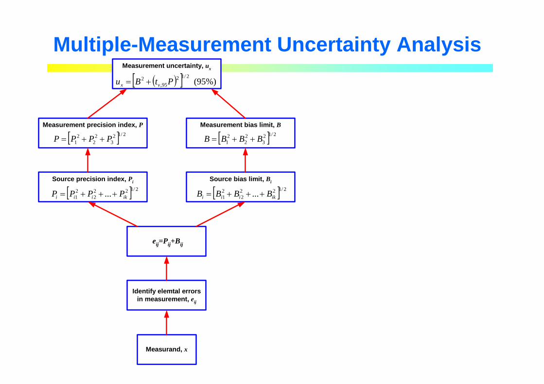
Multiple-Measurement Uncertainty Analysis

Measurand, x

Identify elemtal errorsin measurement, eij

eij=Pij+Bij

Source precision index, Pi Source bias limit, Bi

Measurement bias limit, BMeasurement precision index, P

Measurement uncertainty, ux

[ ] 2/1222

21 ... ikiii BBBB +++=[ ] 2/122

221 ... ikiii PPPP +++=

[ ] 2/123

22

21 PPPP ++= [ ] 2/12

322

21 BBBB ++=

( )[ ] (95%) 2/12

95,2 PtBu vx +=

Measurement bias limit, BMeasurement precision index, P

Measurement uncertainty, ux

Example: After an experiment to measure stress in a load beam, an uncertainty analysis reveals the following source errors in stress measurement whose magnitude were computed from elemental errors

B1 = 1.0 N/cm2 B2 = 2.1 N/cm2 B3 = 0 N/cm2

P1 = 4.6 N/cm2 P2 = 10.3 N/cm2 P3 = 1.2 N/cm2

v1 = 14 v2 = 37 v3 = 8If the mean value of the stress in the measurement is 223.4 N/cm2, determine the best estimate of the stress

Solution: Find uσσσσ

Known: Experimental error source indices

Assume: All elemental error have been included

Multiple-Measurement Uncertainty Analysis

[ ] 2/123

22

21 PPPP ++= [ ] 2/12

322

21 BBBB ++=

( )[ ] (95%) 2/12

95,2 PtBu vx +=

Propagation Uncertainty Analysis to a result

The measurement uncertainty , uR

The degrees of freedom, v

[ ]

[ ]{ }∑

∑

=

=

= L

ixixii

L

ixii

vP

P

v

1

4

2

1

2

/θ

θ

( ) (95%) , 295

2RvRR PtBu +=

∑=

±=L

ixiiR PP

1

2][θ ∑=

±=L

ixiiR BB

1

2][θwhere

Consider the result, R which is determined from the function of the n independent variables xi1, xi2 , xi3, …, xiL

%)( ' PuRR R±=

Example: The density of a gas, ρρρρ, which is believed to follow the ideal gas equation of state, ρρρρ = p/RT, is to be estimated through separate measurements of pressure, p, and temperature, T. the gas is housed with in a rigid impermeable vessel. The literature accompanying the pressure measurement system states an accuracy to within 1% of the reading an that accompanying the temperature measuring system suggest 0.6oR. Twenty measurements of pressure, Np = 20, and ten measurements of temperature, NT = 10, are made with the following statistical outcome:

Where psfa refers to lb/ft2 absolute. Determine a best estimate of the density. The gas constant is R = 54.7 ft lb/lbm

oR

Solution: Find

Known:

Assume: Gas behaves as an ideal gas

Propagation Uncertainty Analysis to a result

psfa 91.2253=p psfa 21.167=pS

R4.560 o=T R0.3 o=TS

Tp STSp ,,,

R lb/lbft 7.54 / om== RRTPρ

ρρρ u+='

Propagation Uncertainty Analysis to a result

( )[ ] (95%) 2/12

95,2 PtBu v+=ρ

( ) ( )22TTpp BBB θθ +±= ( ) ( )22

TTpp PPP θθ +±=

( ) ( )[ ]( ) ( ) TTTppp

TTpp

vPvP

PPv

// 44

222

θθ

θθ

+

+=where

RTpp

1=

∂∂

=ρ

θ

R lb/lbft 7.54 / om== RRTPρ

2RT

p

TT −=∂∂

=ρ

θ

where