Uncertainties in transient capture zones

Velimir V VesselinovHydrology, Geochemistry, and Geology Group Earth and Environmental Sciences (EES-6)Los Alamos National Laboratory, Los Alamos NM 87545, USAvvv@lanl.gov

LA-UR-06-2305CMWR XVI

Computational Methods in Water ResourcesCopenhagen, Denmark, June 19-22 2006

Capture zones

Well 1

Well 2

Source

Background

delineation of capture zones of water supply wells is important for the efficient protection of groundwater resources

capture zones are typically estimated using models

frequently, transients in groundwater flow and their effect on the dispersion of the potential contaminant plumes are ignored in the capture-zone analyses

Capture zone definitions: Steady-state zones are delineated using (future?) steady-state flow

field

Transient zones are delineated using transient flow field:

transients in the flow field

transients in the contaminant releases

instantaneous releases: snapshots of the capturing associated with a given release time

continuous releases: cumulative capturing of contaminants over the release period

t=t2

Impact of transients on contaminant plume

Well 1

Well 2

Well 1

Well 2

Source Source

Contaminant source is within capture zones of both wells … … but steady-state / advective-only capture zone analyses will give us an incorrect result.

t=t1

Methodology 2D synthetic capture-zone analysis

uniform medium

2 wells with temporally varying rates

confined groundwater flow is solved numerically (for convenience); analytical solutions are available as well

capture zones are delineated using forward particle tracking under both advective and advective-dispersive regimes

dimensionless model parameters are derived based on analytical expressions

Codes grid-generation: LaGriT (Trease et al., 1996) flow simulation: FEHM (Zyvoloski et al., 2001) particle-tracking: FEHM (Robinson, 2002)

Model domain

x/d

y/d

-10 -5 0 5 100

2

4

6

8

10

dimensionless coordinates: x/d, y/d, where d is the distance between wells

Region of capture-zone analyses

x/d

y/d

-2 -1 0 1 20

0.5

1

1.5

2

Q

Q

tC

tC

Well 1

Well 2

Temporal variability of pumping rates

tC

tC tC

To reduce the effect of initial conditions, 10 pumping cycles are applied before the analysis of transient capture-zone commences

Dimensionless model parameters pumping rate / advective transport velocity: QtC/(md2φ) [–]

obtained by comparison of quasi-steady-state advective velocity Q/(mdφ) [L/T] and velocity required for a water particle to move distance d for time tC, i.e. d/tC [L/T]

pumping time interval: tCa/d2 [–]

coordinates: x/d, y/d [–]

longitudinal / transverse dispersivities: αL/d, αT/d [–]

where:• k = permeability [L/T]• a = hydraulic diffusivity [L2/T] (a=k/SS, SS=specific storage [L–1] )• Q = pumping rate [L3/T]• tC = pumping time interval [T]• d = distance between the pumping wells [L]• m = aquifer thickness [L]• φ = advective porosity [–]

m = 100 md = 100 mtC = 1000 dQ =1 /sa = 864 m2/dφ = 0.01

Particle-tracking simulation of impacts of transients on the contaminant plumes

Steady-state capture zones

steady-state flow field instantaneous/continuous

releases

In this case, steady-state capture zones are not affected by the uncertainties in the model parameters

LEGEND:RED – capture zone of the left wellBLUE – capture zone of the right well

Transient capture zones

transient flow field instantaneous (after 10 pumping cycles) and continuous releases

Investigated uncertainties

transport velocity hydraulic diffusivity longitudinal/transverse dispersivities release times: instantaneous/continuous

QtC/(md2φ)=0.864

tCa/d2=86.4

QtC/(md2φ)=4.32

QtC/(md2φ)=8.64 QtC/(md2φ)=17.3

Impact of transport velocities

QtC/(md2φ)<0.01

SLOW

FAST

The slower the transport velocities, the higher the number of capture-zone fingers

Steady-state vs transient capture zones

QtC/(md2φ)<0.01tCa/d2=86.4

Transient capture zones obtained for the case of very low transport velocities and steady-state capture zones are equivalent

steady-state

QtC/(md2φ)=8.64

tCa/d2=86.4

tCa/d2=0.864

tCa/d2=864 faster propagation of pressures

confined conditions

Impact of hydraulic diffusivity

The lower the hydraulic diffusivity, the wider the capture-zone fingers

slower propagation of pressures unconfined conditions

Impact of dispersion

αL/d =0.1αT/d =0.01

QtC/(md2φ)=8.64tCa/d2=86.4

Low velocity (Steady-state) High velocity

LEGEND:Color range between RED and BLUE represents the capturing percentage

QtC/(md2φ)<0.01tCa/d2=86.4

Transient capture zones:Impact of longitudinal/transverse dispersivities

QtC/(md2φ)=8.64tCa/d2=86.4

αL/d =0.1αT/d =0.01

αL/d =0.1αT/d =0.001

αL/d =0.1αT/d =0.1

αL/d =0.01αT/d =0.01

In the high velocity transient case, αL is important, while αThas a minor effect on the estimates

Low-velocity transient (steady-state) capture zones:Impact of longitudinal/transverse dispersivities

αL/d =0.1αT/d =0.01

αL/d =0.1αT/d =0.001

αL/d =0.01αT/d =0.01

αL/d =0.1αT/d =0.1

In the low-velocity transient (steady-state) case, αT is important, while αL has a minor effect on the estimatesQtC/(md2φ)<0.01

tCa/d2=86.4

Transient capture zones:Impact of release times

QtC/(md2φ)=8.64tCa/d2=86.4

Q

Q

tC

tC

Well 1

Well 2tC

tC tC

Capture zones change with the release time

Transient capture zones:Impact of release times

QtC/(md2φ)=8.64tCa/d2=86.4

Q

Q

tC

tC

Well 1

Well 2tC

tC tC

Animation of transient capture zones at different release times

Transient capture zones:Continuous releases

QtC/(md2φ)=8.64tCa/d2=86.4

Smearing of the capture zones due to continuous releases

LEGEND:Color range between RED and BLUE represents the capturing percentage

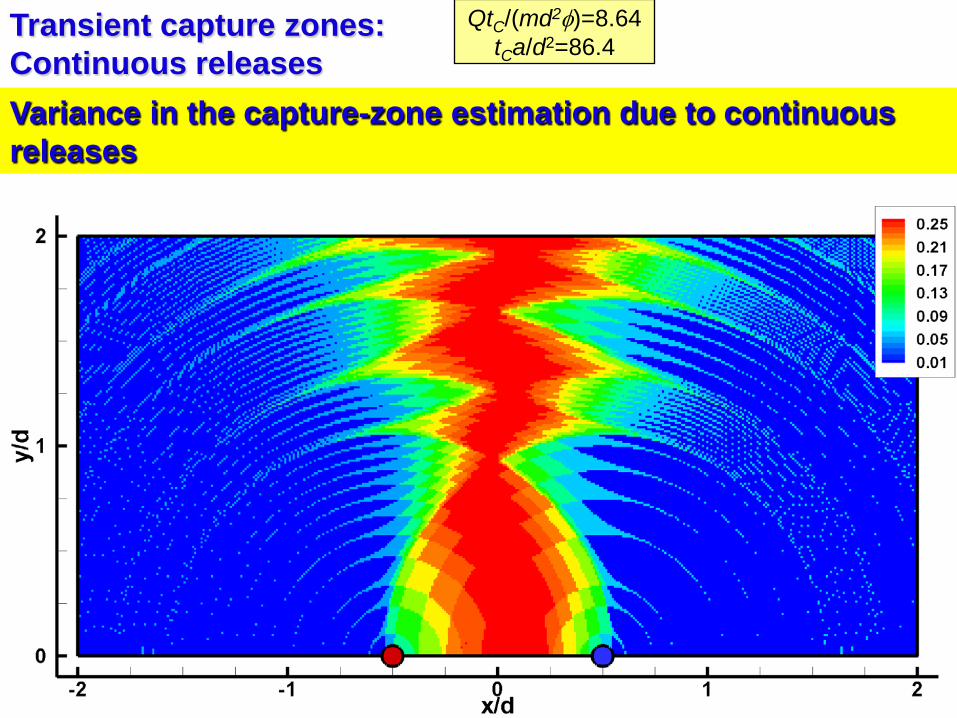
QtC/(md2φ)=8.64tCa/d2=86.4

Transient capture zones:Continuous releasesVariance in the capture-zone estimation due to continuous releases

0

10

20

30

40

50

60

1947

1949

1951

1953

1955

1957

1959

1961

1963

1965

1967

1969

1971

1973

1975

1977

1979

1981

1983

1985

1987

1989

1991

1993

1995

1997

1999

2001Year

Pum

ping

rate

[kg/

s]

PM-1

PM-2

PM-3

PM-4

PM-5

O-1

O-4

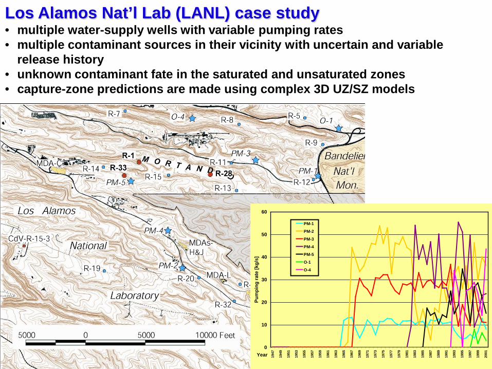
Los Alamos Nat’l Lab (LANL) case study• multiple water-supply wells with variable pumping rates• multiple contaminant sources in their vicinity with uncertain and variable

release history• unknown contaminant fate in the saturated and unsaturated zones• capture-zone predictions are made using complex 3D UZ/SZ models

PM5

PM4

PM3

PM2

O4

x [m]

y[m

]

16000 18000 20000 22000

-132000

-131000

-130000

-129000

-128000

-127000O-1O-4PM-1PM-2PM-3PM-4PM-5MortanPM-5PM-4PM-3PM-2PM-1O-4O-1

Mortandad Canyon

Transient capture zones at the water-table

PM5

PM4

PM3

PM2

O4

x [m]

y[m

]

16000 18000 20000 22000

-132000

-131000

-130000

-129000

-128000

-127000

number of wells54321

Mortandad Canyon

Number of wells capturing contamination from each location

Transient capture zones at the water-table

Findings/Conclusions Transients are important to consider in capture zone analyses

Significance of transients for capture-zone analyses depends on amplitude/frequency of the transients in the groundwater flow

and transport (well pumping/contaminant releases), rate of propagation of contaminants (pore velocities) contaminant dispersion (dispersivities) rate of propagation of hydraulic pressures (hydraulic diffusion)

Uncertainties in the transient capture zone estimates depend predominantly on: transport velocities longitudinal dispersivity in the case of high transport velocities,

and transverse dispersivity in the case of low transport velocities release times

Transient capture zones can be effectively delineated even for very complex models through parallelization