umbayesadaptintro sm2
DESCRIPTION
Bayesian Clinical TrialsTRANSCRIPT

Introduc)on to Bayesian Adap)ve Methods
Lecture notes modified from Dr. Melanie Quintana, Fall, 2013

Common Trial: How do I get to work?

Common Trial: How do I get to work?
• Start a new job and need to figure out the fastest way to get to work – Could take the highway – Could take the back roads
• How do you decide which way to go? • How do you decide how to decide?

Common Trial: How do I get to work?
– Put 30 envelopes in your car where each has one of 3 routes wriPen on the inside. Randomly select an envelope each morning and drive that route. Record drive )me and at the end of the 30 days choose the route with the quickest average drive )me.
– Drive one route on the first day. Make note of how long it took you. Drive a different route the next day. If it took you longer than the first route you switch back to driving the first route the next day……

Common Trial: How do I get to work?
• Adap)ve aspects of fastest route trial? – Adap)ve Randomiza)on
• If one route took too long once you tried it you would be less likely to try it again.
– Arm Dropping • If a route took WAY too long then you may want to drop it all together from your op)ons and never take it again
– Early Stopping • How long un)l you had enough “data” to convince you of the fastest route?

Example: RESPECT Trial
• Inves)gate whether the closure of pa)ent foramen ovale (PFO) using the Amplatzer PFO Occluder is superior to medical therapy in preven)ng stroke
• Randomized 1:1 to closure and medical therapy groups • Original Design: – Report primary results once 25 events (strokes) had been observed
– If 19 or more of these strokes were in the medical therapy group declare success!
– Es)mated 80% power to show a reduc)on in risk with closure of approximately 75%

Example: RESPECT Trial
• An)cipated Regret – Imagine that we run the trial and it is a near miss… – What reasons can you see that would have made it unsuccessful?

Example: RESPECT Trial
• Data at )me of primary analysis – 980 pa)ents enrolled in the study across 69 sites
• 499 in the device group • 481 in the control group
– 851 (86.8%) remained in ac)ve follow-‐up • dropout rate was 9.2% in the closure group • 17.2% in the medical therapy group
– In the inten)on-‐to-‐treat cohort, there were 9 events in the device group and 16 events in the control group. • Inves)gators were not able to claim success

Example: RESPECT Trial
0 2 4 6 8
0.80
0.85
0.90
0.95
1.00
Years to Event
Even
t−fre
e Pr
obab
ility
Device Group(n=9)
Control Group(n=16)
HR, 0.49 (95% CI, 0.20−1.08)Post. Prob. HR < 1 = 96%

Example: RESPECT Trial
• What went wrong? – Differen)al drop out: Many of the pa)ents in the medical therapy group dropped out of the study or went to the closure group
– Does not appear to be a closure benefit within the first year • Biological reasoning behind this: takes )me for the hole to close

Example: RESPECT Trial
• What could we have done differently? – Allow the data to tell us when to stop – Posterior probability that closure was superior to medical therapy (HR <1) at )me of primary analysis was 0.96.
– Would you have chosen to stop the trial?

What are Adap)ve Designs?
• Adap)ve Design – A design that “changes” depending on observed values in the trial
• Prospec)ve Adap)ve Design – A design that has pre-‐specified dynamic aspects that are determined by the accruing informa)on
• Every )me I say “Adap)ve Design” I mean “Prospec)vely Adap)ve Design”

What are Adap)ve Trials? • Trials in which key design parameters change during trial execu)on based upon a priori predefined rules and accumula)ng data from the trial to achieve goals of validity, scien)fic efficiency, and safety
– Planned: All possible adapta)ons defined a priori – Well-‐defined: Criteria for adap)ng clearly explained – Key parameters: Not minor inclusion or exclusion criteria, rou)ne amendments, etc.
– Validity: Reliable sta)s)cal inference

What are Adap)ve Trials? Trials that change based on prospec3ve rules & the accruing informa3on • Adap)ve sample sizes based on predic)ve probabili)es
– Stop early for success – Terminate early for fu)lity
• Adap)ve randomiza)on – For sta)s)cal efficiency – For improved pa)ent treatment – Drop/Re-‐enter arms or dose groups
• Adapt to responding sub-‐popula)ons • Adap)ve borrowing of informa)on • Seamless Phase 2/3 Designs

• Drug already approved in Japan but not in the US.
• It seems efficacious there, but the popula)on here might be different.
• For the sake of pa)ents we start randomizing 3:1 so most pa)ents get something we think is effec)ve. • We incorporate borrowing from the Japanese trial to effec)vely increase the control popula)on. But if the control group here has a different rate than in Japan, maybe we borrow less and even change the randomiza)on probability here back to 2:1 or even 1:1.

Typical Prospec)ve Adap)ve Design
Analyze Available Data
Continue Data Collection
Begin Data Collection with Initial Allocation and Sampling Rules
Stopping Rule Met?
Stop Trial or Begin Next Phase in Seamless
Design
Revise Allocation and Sampling Rules
per Adaptive Algorithm

Adap)ve Advantages
• Companies save resources and successful drugs/devices get to market faster – Stop a trial early if it is most likely fu)le and move on to the next promising drug/device
– Stop a trial early for success • More pa)ents get treated with the bePer drug /device during the trial – Would you rather be the last pa)ent enrolled in a clinical trial or the first person treated aper its results are published?

Adap)ve Design Tools Using Bayesian tools to help us design the trial? • Posterior Probability
– Probability that the drug is effec)ve given the data you have seen so far – Probability that the dose is the maximum effec)ve dose given the data
you have seen so far • Can use these to allocate pa)ents and to declare success
• Predic/ve Probability – Probability trial will be successful aper outstanding data you have not yet
observed – Can help us determine the likelihood that a trial will be successful before
it even starts • Example… will our Phase 3 trial be successful given our Phase 2 data??
– Help us decide if we want to stop the currently enrolling trial due to fu)lity
• Clinical Trial Simula/ons – Simula)ons of scenarios of how the trial could go – Help us test our design

−4 −2 0 2 4
0.0
0.1
0.2
0.3
0.4
What is Bayesian?
Frequen/st • θ is an unknown constant
• If the true mean, θ, were 0, how likely is
2? Pr X |θ = 0( )
X ~ N θ ,12( )

What is Bayesian?
Bayesian
• θ is a random variable!
• What is the distribu)on of θ aper observing X?
X ~ N θ ,12( )
Pr θ | X( )

What is Bayesian?
• How do we get there? – From to ?
• Bayes Theorem (the theorem of Inverse Probability) is the “crank” that gets from Pr(A|B) to Pr(B|A)
X ~ N θ ,12( ) Pr θ | X( )
Pr B | A( ) = Pr A | B( )Pr B( )Pr A | B( )Pr B( ) + Pr A | BC( )Pr BC( )

What is Bayesian?
Pr B | A( ) = Pr A | B( )Pr B( )Pr A | B( )Pr B( ) + Pr A | BC( )Pr BC( )
Prior Probability
Likelihood (data)
Posterior Probability
Prior Beliefs + Data = Posterior Probability

Simple Bayes Example
• Coin, Pr(HEADS) = π • π = 0.25 or π =0.75, equally likely. • DATA: Flip coin twice, both heads. • π ???

Simple Bayes Example
=0.75( )2 0.5( )
0.75( )2 0.5( ) + 0.25( )2 0.5( )
= 0.90
Pr B | A( ) = Pr A | B( )Pr B( )Pr A | B( )Pr B( ) + Pr A | BC( )Pr BC( )
Pr p = 0.75 |DATA( )
=Pr DATA | p = 0.75( )Pr p = 0.75( )
Pr DATA | p = 0.75( )Pr p = 0.75( ) + Pr DATA | p = 0.25( )Pr p = 0.25( )

Bayes Rule More Generally
• For our simple example θ= π • Don’t really just have two op)ons – π = 0.25 or π =0.75 – π = any con)nuous value from 0 to 1
π θ | X( ) = L X |θ( )π θ( )L X |θ( )π θ( )dθ∫

Bayes Rule More Generally
0.0 0.4 0.8
01
23
4
Prior Beta(1,1)
Pi
Den
sity
0.0 0.4 0.8
01
23
4
After S
Pi
Den
sity
0.0 0.4 0.8
01
23
4
After SS
Pi
Den
sity
0.0 0.4 0.8
01
23
4
After SSF
Pi
Den
sity
0.0 0.4 0.8
01
23
4
After SSFS
Pi
Den
sity
0.0 0.4 0.8
01
23
4
After SSFSF
Pi
Den
sity
0.0 0.4 0.8
01
23
4
After SSFSFS
Pi
Den
sity
0.0 0.4 0.8
01
23
4
After SSFSFSS
Pi
Den
sity
0.0 0.4 0.8
01
23
4
After SSFSFSSSFSSSSSSFS
Pi
Den
sity

Interac)ve Drug Development Example
• Suppose in Phase II, with 20 pa)ents on Dose 2, we saw 6 successes and 14 failures
• Assume a prior distribu)on for Pr(Response) (p) of beta(1,1)
• What is the posterior distribu)on of p? – What is the posterior probability p>.20 – 95 % probability that the response rate is between ___ and ___?

Posterior Probability
!!
Data|p~Bin(6,20)p~Beta(1,1)p|Data~? !!
Beta(a,b)= Γ(a+b)Γ(a)Γ(b) x
(a−1)(1− x)(b−1)
Γ(a)= (a−1)!
!!
pr(p|Data)∝pr(Data|p)pr(p)
∝ 206
⎛
⎝⎜⎞
⎠⎟p6(1− p)14
∝ 20!6!14!p
6(1− p)14
∝ Γ(21)Γ(7)Γ(15)p
(7−1)(1− p)(15−1)
!!Beta(7,15)

Posterior Probability
0.0 0.2 0.4 0.6 0.8 1.0
01
23
4
Prior Distributionp~Beta(1,1)
p
Density
0.0 0.2 0.4 0.6 0.8 1.0
01
23
4
Posterior Distributionp|data~Beta(7,15)
p
Density

01
23
4
Posterior Prob. Response Rate > .20
p
Density
0.0 0.2 1.0
Posterior Probability
Pr(p>.20|6S and 14F) = 0.89

Posterior Probability 0
12
34
Posterior 95% CI
p
Density
0.15 0.520.0 1.0
Interac)ve Drug Development Example
• With 20 pa)ents on Dose 2 we saw 6 successes and 14 failures
• Assume a prior distribu)on for Pr(Response) (p) of beta(1,1)
• What is the posterior distribu)on of p? • What is the predic)ve probability of success in 300 pa)ent Phase 3 given this data?

Predic)ve Probability
• If we have 74 or more successes out of 300 we will win Phase 3 (alpha = .025)
• How likely is it that we will see 74 or more successes given data we have seen so far?
• What is the the distribu)on of future data given data we have seen so far?

Predic)ve Probability
• Simulate a (p | data) from beta(7,15) • Simulate an (x | p) from bin(300,p) • Distribu)on of x’s is beta-‐binomial – the predic)ve distribu)on – Can count the propor)on of these x’s that are greater than or equal to 74 to get the predic)ve probability of success in Phase 3
Pr(x | data) = pr(x | p) pr(p | data) dp∫=
300x
⎛⎝⎜
⎞⎠⎟∫ px 1− p( )300−x Γ(22)
Γ 7( )Γ(15) p7−1 1− p( )15−1 dp
Beta-‐Binomial Dist

0 50 100 150 200 250 300
0.00
0.01
0.02
0.03
0.04
0.05
Binomial Distributionp=6/20
Number Successes Phase III
Den
sity
0 50 100 150 200 250 300
0.00
0.01
0.02
0.03
0.04
0.05
Predictive Distributionp~Beta(7,15)
Number Successes Phase III
Den
sity
Condi)onal Probability vs. Predic)ve Probability
0.75
0.98

• Beta-‐binomial has much more variability… we are much less confident that we will be successful in phase 3 than if we would have just assumed the response rate was 6/20 (= 0.3) and found the condi)onal power in phase 3 given this response rate!
• What does the predic)ve probability look like if we recruit an addi)onal 20 and we see we see 12/40 at our next interim analysis?

0 50 100 150 200 250 300
0.00
0.01
0.02
0.03
0.04
0.05
Binomial Distributionp=12/40
Number Successes Phase III
Den
sity
0 50 100 150 200 250 300
0.00
0.01
0.02
0.03
0.04
0.05
Predictive Distributionp~Beta(13,29)
Number Successes Phase III
Den
sity
Condi)onal Probability vs. Predic)ve Probability
0.80
0.98

• Same condi)onal power (since we are condi)oning on same value of p=0.3) but predica)ve power changes even though the es)mate of the response rate does not change!
• Predic)ve power takes into considera)on how much data we have seen and how certain we are of the response rate.

0 50 100 150 200 250 300
0.00
0.01
0.02
0.03
0.04
0.05
Binomial Distributionp=30/100
Number Successes Phase III
Den
sity
0 50 100 150 200 250 300
0.00
0.01
0.02
0.03
0.04
0.05
Predictive Distributionp~Beta(31,101)
Number Successes Phase III
Den
sity
Condi)onal Probability vs. Predic)ve Probability
0.87
0.98

Bayesian Advantages to Trial Design
• Provide Intui)ve Inference – Posterior probability of treatment effect – Posterior probability that the es)mate of the treatment effect is
in some interval – What most people think their frequen)st confidence intervals and
p-‐values are telling them • Provide predic)ve probabili)es of success before and during
trials – Take into account uncertainty of the treatment effect – Change based on how much data we have seen
• Synthesis of Evidence – Mul)ple sources of informa)on can be combined (previous trials) – Expert opinion can play a role in inference

Trial Simula)on
• For complex adap)ve designs you can not calculate opera)ng characteris)cs analy)cally (Type I Error and Power)
(integra)on can not be done in closed form) • Simula)on the only way to do this…

Interac)ve Drug Development
• An example in drug development considering molecule with unknown effect to assess in a dose finding Phase 2 trial. – 3 doses of the molecule
• The goal of the trial will be to determine if the molecule should be developed in Phase 3, and if so which dose should be developed. – The company will have resources for a 300 pa)ent Phase 3 trial
• Your goal is to design their Phase 2 trial in stages, adap)ng the number of pa)ents assigned to each dose aper each stage.

Interac)ve Drug Development
• Primary Endpoint: – Dose efficacy (0 = no response, 1 = beneficial response)
• An effec)ve dose is any dose that has Pr(response) >= 20%
• Note that in a 300 person trail, we “win” the trial if we observe at least 74 responses.

Interac)ve Drug Development
• Thus there are 300 pa)ents to allocate to the dose arms of your choice. – The trial is divided into 5 groups of 60 pa)ents, recruited sequen)ally
– There are 4 interim analyses where you will get efficacy data and will have to decide one of three things: • Terminate the trial for fu)lity • Stop the trial for success, pick dose and advance to Phase 3 tes)ng
• Con)nue to collect data, alloca)ng the next 60 pa)ents.

Simula)on of Interac)ve Drug Development
• Example Prospec)ve Design: – Interim analysis every 60 pa)ents – Begin adap)ve alloca)on aper we see first 60 pa)ents • Sample pa)ents based on probability that each dose is “best”
• “best” dose is defined as the dose that provides that highest response rate
– Propose to stop for fu)lity if predic)ve probability of success in Phase III for max dose is < 0.10
– Propose to stop for early success if predic)ve probability of success in Phase III for max dose is >.95

Simula)on of Interac)ve Drug Development: N=60
*Start with 20 pa)ents on each dose
*Low probability Dose 1 is max
●
● ●
0.0
0.2
0.4
0.6
0.8
1.0
Pr(Response)
Dose
Pr(R
espo
nse)
−
− −
−
− −
1 2 3 1 2 3
Subject Allocation
Dose
Num
ber o
f Sub
ject
s
050
100
150
200
1 2 3
Prob. Dose has Max Response
Dose
Prob
abilit
y
0.0
0.2
0.4
0.6
0.8
1.0
1 2 3
PPS in Phase III
Dose
Prob
abilit
y
0.0
0.2
0.4
0.6
0.8
1.0

Simula)on of Interac)ve Drug Development: N=120
*Do not allocate many new pa)ents to dose 1
●
●●
0.0
0.2
0.4
0.6
0.8
1.0
Pr(Response)
Dose
Pr(R
espo
nse)
−
− −
−
−−
1 2 3 1 2 3
Subject Allocation
Dose
Num
ber o
f Sub
ject
s
050
100
150
200
1 2 3
Prob. Dose has Max Response
Dose
Prob
abilit
y
0.0
0.2
0.4
0.6
0.8
1.0
1 2 3
PPS in Phase III
Dose
Prob
abilit
y
0.0
0.2
0.4
0.6
0.8
1.0

Simula)on of Interac)ve Drug Development: N=180
*Stop for success if PPS in Phase III is >.95 for max dose
●
●
●
0.0
0.2
0.4
0.6
0.8
1.0
Pr(Response)
Dose
Pr(R
espo
nse)
−
−−
−
−
−
1 2 3 1 2 3
Subject Allocation
Dose
Num
ber o
f Sub
ject
s
050
100
150
200
1 2 3
Prob. Dose has Max Response
Dose
Prob
abilit
y
0.0
0.2
0.4
0.6
0.8
1.0
1 2 3
PPS in Phase III
Dose
Prob
abilit
y
0.0
0.2
0.4
0.6
0.8
1.0
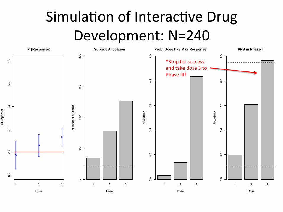
Simula)on of Interac)ve Drug Development: N=240
*Stop for success and take dose 3 to Phase III!
●
●
●
0.0
0.2
0.4
0.6
0.8
1.0
Pr(Response)
Dose
Pr(R
espo
nse)
−
−
−
−
−
−
1 2 3 1 2 3
Subject Allocation
Dose
Num
ber o
f Sub
ject
s
050
100
150
200
1 2 3
Prob. Dose has Max Response
Dose
Prob
abilit
y
0.0
0.2
0.4
0.6
0.8
1.0
1 2 3
PPS in Phase III
Dose
Prob
abilit
y
0.0
0.2
0.4
0.6
0.8
1.0

Simula)on of Interac)ve Drug Development
• What scenarios should we simulate under?

Simula)on of Interac)ve Drug Development
• What scenarios should we simulate under?
Pr(Response)
Dose 1 Dose 2 Dose 3
All Null .2 .2 .2
All Good Max Max Max
One Good .2 .2 Max
Increase .2 1/2Max + .1 Max
• Max Response Rate? – .3,.4,.5
Simula)on of Interac)ve Drug Development
• What opera)ng characteris)cs should we report?

Simula)on of Interac)ve Drug Development
• What opera)ng characteris)cs should we report? – Probability of stopping for success or for fu)lity • Early or Late?

Simula)on of Interac)ve Drug Development
• What opera)ng characteris)cs should we report? – Probability of stopping for success or for fu)lity • Early or Late?
– Mean subjects used • On average how many pa)ents did we use

Simula)on of Interac)ve Drug Development
• What opera)ng characteris)cs should we report? – Probability of stopping for success or for fu)lity • Early or Late?
– Mean subjects used • On average how many pa)ents did we use
– Mean dura)on of trial • On average how many interims did it take us to either stop for success or fu)lity
– Probability each dose was chosen as the “best”

Simula)on of Interac)ve Drug Development
Prob. of Success
Prob. of Fu/lity
Mean Subjects
Mean Dura/on
Prob. Dose is Best
Scenario Max Response Dose 1 Dose 2 Dose 3
All Null (.2-‐.2-‐.2)
.2 0.04 0.13 280.56 4.68 0.34 0.31 0.35
All Good (Max-‐Max-‐Max)
.3 0.82 0.00 162.12 2.70 0.37 0.32 0.31
.4 1.00 0.00 75.60 1.26 0.32 0.34 0.34
.5 1.00 0.00 61.08 1.02 0.34 0.33 0.33
One Good (.2-‐.2-‐Max)
.3 0.49 0.01 231.30 3.86 0.04 0.06 0.91
.4 0.99 0.00 112.86 1.88 0.01 0.00 0.98
.5 1.00 0.00 76.20 1.27 0.01 0.00 0.99
Increase (.2-‐.5Max+.1-‐Max)
.3 0.52 0.02 223.44 3.72 0.04 0.00 0.96
.4 0.99 0.00 108.00 1.80 0.01 0.00 0.99
.5 1.00 0.00 76.80 1.28 0.00 0.00 1.00

Simula)on of Interac)ve Drug Development
• What are the moving parts that we may want to fine tune? – PPS threshold for success: • Are we sending too many null trials to Phase 3? • Are we not sending enough successful trials?

Simula)on of Interac)ve Drug Development
Prob. of Success
Prob. of Fu/lity
Mean Subjects
Mean Dura/on
Prob. Dose is Best
Scenario Max Response Dose 1 Dose 2 Dose 3
All Null (.2-‐.2-‐.2)
.2 0.04 0.13 280.56 4.68 0.34 0.31 0.35
All Good (Max-‐Max-‐Max)
.3 0.82 0.00 162.12 2.70 0.37 0.32 0.31
.4 1.00 0.00 75.60 1.26 0.32 0.34 0.34
.5 1.00 0.00 61.08 1.02 0.34 0.33 0.33
One Good (.2-‐.2-‐Max)
.3 0.49 0.01 231.30 3.86 0.04 0.06 0.91
.4 0.99 0.00 112.86 1.88 0.01 0.00 0.98
.5 1.00 0.00 76.20 1.27 0.01 0.00 0.99
Increase (.2-‐.5Max+.1-‐Max)
.3 0.52 0.02 223.44 3.72 0.04 0.00 0.96
.4 0.99 0.00 108.00 1.80 0.01 0.00 0.99
.5 1.00 0.00 76.80 1.28 0.00 0.00 1.00

Simula)on of Interac)ve Drug Development
• What are the moving parts that we may want to fine tune? – PPS threshold for success: • Are we sending too many null trials to Phase 3? • Are we not sending enough successful trials?
– PPS threshold for fu)lity: • Are we stopping a trial that may go on to be successful? • Are we not stopping enough null trials?

Simula)on of Interac)ve Drug Development
Prob. of Success
Prob. of Fu/lity
Mean Subjects
Mean Dura/on
Prob. Dose is Best
Scenario Max Response Dose 1 Dose 2 Dose 3
All Null (.2-‐.2-‐.2)
.2 0.04 0.13 280.56 4.68 0.34 0.31 0.35
All Good (Max-‐Max-‐Max)
.3 0.82 0.00 162.12 2.70 0.37 0.32 0.31
.4 1.00 0.00 75.60 1.26 0.32 0.34 0.34
.5 1.00 0.00 61.08 1.02 0.34 0.33 0.33
One Good (.2-‐.2-‐Max)
.3 0.49 0.01 231.30 3.86 0.04 0.06 0.91
.4 0.99 0.00 112.86 1.88 0.01 0.00 0.98
.5 1.00 0.00 76.20 1.27 0.01 0.00 0.99
Increase (.2-‐.5Max+.1-‐Max)
.3 0.52 0.02 223.44 3.72 0.04 0.00 0.96
.4 0.99 0.00 108.00 1.80 0.01 0.00 0.99
.5 1.00 0.00 76.80 1.28 0.00 0.00 1.00

Simula)on of Interac)ve Drug Development
• Example Change in Prospec)ve Design: – Interim analysis every 60 pa)ents – Begin adap)ve alloca)on aper we see first 60 pa)ents • Sample pa)ents based on probability that each dose is the max
– Propose to stop for fu)lity if predic)ve probability of success in Phase III for max dose is < 0.15
– Propose to stop for success if predic)ve probability of success in Phase III for max dose is >.90

Simula)on of Interac)ve Drug Development
Prob. of Success
Prob. of Fu/lity
Mean Subjects
Mean Dura/on
Prob. Dose is Best
Scenario Max Response Dose 1 Dose 2 Dose 3
All Null (.2-‐.2-‐.2)
.2 0.12 0.25 253.20 4.22 0.34 0.32 0.34
All Good (Max-‐Max-‐Max)
.3 0.93 0.00 116.46 1.94 0.33 0.33 0.35
.4 1.00 0.00 63.96 1.07 0.32 0.36 0.32
.5 1.00 0.00 60.12 1.00 0.35 0.31 0.34
One Good (.2-‐.2-‐Max)
.3 0.70 0.02 181.02 3.02 0.08 0.07 0.86
.4 1.00 0.00 93.72 1.56 0.02 0.02 0.96
.5 1.00 0.00 67.92 1.13 0.01 0.01 0.98
Increase (.2-‐.5Max+.1-‐Max
.3 0.69 0.03 183.18 3.05 0.09 0.00 0.91
.4 1.00 0.00 93.84 1.56 0.02 0.00 0.98
.5 1.00 0.00 67.56 1.13 0.01 0.00 0.99

Clinical Trial Simula)on We simulate trials to see how our adap3ve design machine works • Scenarios
– Stress test the machine under different assumed truths (drug doesn’t work, drug is really good, etc…)
• Sample Trials – Watch progress of a virtual trial. The real trial should not be the first )me
your design is run – Don’t want surprises during the trial – Great for debugging (even when you think it’s right) – Great way to illustrate the adap)ve process to collaborators,
management, IRBs, DMCs, investors, etc. • Opera)ng Characteris)cs
– Aggregate results of many sample trials under many different scenarios to get an overall picture of how the design will perform
– Usually have to control Type I error rate by trial & error • Set cri)cal value, run 1,000 sims, check Type I error • Adjust to get Type I error in worst case scenario at 2.5% or 5%