UMAP: Uniform ManifoldApproximation and Projection for

Dimension Reduction

Leland McInnes and John HealyTu�e Institute for Mathematics and Computing

leland.mcinnes@gmail.com jchealy@gmail.com

February 13, 2018

Abstract

UMAP (Uniform Manifold Approximation and Projection) is a novelmanifold learning technique for dimension reduction. UMAP is constructedfrom a theoretical framework based in Riemannian geometry and algebraictopology. �e result is a practical scalable algorithm that applies to realworld data. �e UMAP algorithm is competitive with t-SNE for visual-ization quality, and arguably preserves more of the global structure withsuperior run time performance. Furthermore, UMAP as described has nocomputational restrictions on embedding dimension, making it viable as ageneral purpose dimension reduction technique for machine learning.

1 IntroductionDimension reduction seeks to produce a low dimensional representation of highdimensional data that preserves relevant structure (relevance o�en being appli-cation dependent). Dimension reduction is an important problem in data sciencefor both visualization, and as a potential pre-processing step for machine learn-ing.

As a fundamental technique for both visualization and preprocessing, dimen-sion reduction is being applied in a broadening range of �elds and on ever in-creasing sizes of datasets. It is thus desirable to have an algorithm that is bothscalable to massive data and able to cope with the diversity of data available. Di-mension reduction algorithms tend to fall into two categories; those that seek topreserve the distance structure within the data or those that favor the preserva-tion of local distances over global distance. Algorithms such as PCA [8], MDS

1

arX

iv:1

802.

0342

6v1

[st

at.M

L]

9 F

eb 2

018

[9], and Sammon mapping [20] fall into the former category while t-SNE [15][26], Isomap [24], LargeVis [22], Laplacian eigenmaps [1] [2], di�usion maps [4],NeRV [28], and JSE [12] all fall into the la�er category.

UMAP (Uniform Manifold Approximation and Projection) seeks to provideresults similar to t-SNE but builds upon mathematical foundations related to thework of Belkin and Niyogi on Laplacian eigenmaps. In particular, we seek toaddress the issue of uniform distributions on manifolds through a combinationof Riemannian geometry and the work of David Spivak [21] in category theoreticapproaches to geometric realization of fuzzy simplicial sets.

In this paper we introduce a novel manifold learning technique for dimen-sion reduction. We provide a sound mathematical theory grounding the tech-nique and a practical scalable algorithm that applies to real world data. t-SNE isthe current state-of-the-art for dimension reduction for visualization. Our algo-rithm is competitive with t-SNE for visualization quality and arguably preservesmore of the global structure with superior run time performance. Furthermore,UMAP’s topological foundations allow it to scale to signi�cantly larger data setsizes than are feasible for t-SNE. Finally, UMAP has no computational restric-tions on embedding dimension, making it viable as a general purpose dimensionreduction technique for machine learning.

In section 2 we describe the theory underlying the algorithm. In section 3 weprovide practical results on real world datasets.

2 �e UMAP algorithmIn overview, UMAP uses local manifold approximations and patches togethertheir local fuzzy simplicial set representations. �is constructs a topological rep-resentation of the high dimensional data. Given a low dimensional representa-tion of the data, a similar process can be used to construct an equivalent topolog-ical representation. UMAP then optimizes the layout of the data representationin the low dimensional space, minimizing the cross-entropy between the twotopological representations.

�e construction of fuzzy topological representations can be broken downinto the two problems: approximating a manifold on which the data is assumedto lie; and constructing a fuzzy simplicial set representation of the approximatedmanifold. In explaining the algorithm we will �rst discuss the method of approx-imating the manifold for the source data. Next we will discuss how to constructa fuzzy simplicial set structure from the manifold approximation. We will then

2

discuss the construction of the fuzzy simplicial set associated to a low dimen-sional representation (where the manifold is simply Rd), and how to optimizethe representation. Finally we will discuss some of the implementation issues.

2.1 Uniformdistribution of data on amanifold and geodesicapproximation

�e �rst step of our algorithm is to �nd an estimate of the manifold we assumethe data lies on. �e manifold may be known apriori (as simply Rn) or mayneed to be inferred from the data. Suppose the manifold is not known in ad-vance and we wish to approximate geodesic distance on it. Let the input data beX = {X1, . . . , XN}. As in the work of Belkin and Niyogi on Laplacian eigen-maps [1] [2], for theoretical reasons it is bene�cial to assume that the data isuniformly distributed on the manifold. In practice, real world data is rarely sonicely behaved. However, if we assume that the manifold has a Riemannian met-ric not inherited from the ambient space, we can �nd a metric such that the datais approximately uniformly distributed with regard to that metric.

Formally, letM be the manifold we assume the data to lie on, and let g bethe Riemannian metric onM. �us, for each point p ∈M we have gp, an innerproduct on the tangent space TpM.

Lemma 1. Let (M, g) be a Riemannianmanifold in an ambientRn, and let p ∈Mbe a point. If g is locally constant about p in an open neighbourhoodU such that g isa constant diagonal matrix in ambient coordinates, then in a ball B ⊆ U centeredat p with volume πn/2

Γ(n/2+1)with respect to g, the geodesic distance from p to any

point q ∈ B is 1rdRn(p, q), where r is the radius of the ball in the ambient space and

dRn is the existing metric on the ambient space.

Proof. Let x1, . . . , xn be the coordinate system for the ambient space. A ball BinM under Riemannian metric g has volume given by∫

B

√det(g)dx1 ∧ · · · ∧ dxn.

If B is contained in U , then g is constant in B and hence√

det(g) is constantand can be brought outside the integral. �us, the volume of B is

√det(g)

∫B

dx1 ∧ ... ∧ dxn =√det(g)

πn/2rn

Γ(n/2 + 1),

3

where r is the radius of the ball in the ambient Rn. If we �x the volume of theball to be πn/2

Γ(n/2+1)we arrive at the requirement that

det(g) =1

r2n.

Now, since g is assumed to be diagonal with constant entries we can solve for gitself as

gij =

1r2

if i = j,

0 otherwise. (1)

�e geodesic distance onM under g from p to q (where p, q ∈ B) is de�ned as

infc∈C

∫ b

a

√g(c(t), c(t))dt,

where C is the class of smooth curves c onM such that c(a) = p and c(b) = q,and c denotes the �rst derivative of c onM. Given that g is as de�ned in (1) wesee that this can be simpli�ed to

1

rinfc∈C

∫ b

a

√〈c(t), c(t)〉dt

=1

rinfc∈C

∫ b

a

‖c(t)‖dt

=1

rdRn(p, q)

(2)

If we assume the data to be uniformly distributed onM (with respect to g)then any ball of �xed volume should contain approximately the same number ofpoints ofX regardless of where on the manifold it is centered. Conversely, a ballcentered at Xi that contains exactly the k-nearest-neighbors of Xi should have�xed volume regardless of the choice of Xi ∈ X . Under Lemma 1 it follows thatwe can approximate geodesic distance from Xi to its neighbors by normalisingdistances with respect to the distance to the kth nearest neighbor of Xi.

In essence, by creating a custom distance for each Xi, we can ensure thevalidity of the assumption of uniform distribution on the manifold assumption.�e cost is that we now have an independent notion of distance for each and

4

every Xi, and these notions of distance may not be compatible. �at is, we havea family of discrete metric spaces (one for each Xi) that we wish to merge into aconsistent global structure. �is can be done in a natural way by converting themetric spaces into fuzzy simplicial sets.

2.2 Fuzzy topological representationWe will convert to fuzzy topological representations as means to merge the in-compatible local views of the data. �e topological structure of choice is that ofsimplicial sets. For more details on simplicial sets we refer the reader to [7] and[6]. Our approach draws heavily upon the work of David Spivak in [21], andmany of the de�nitions and theorems below are drawn from those notes.

De�nition 1. �e category ∆ has as objects the �nite order sets [n] = {1, . . . , n},with morphims given by (non-strictly) order-preserving maps.

De�nition 2. A simplicial set is a functor from ∆op to Sets, the category of sets.

Simplicial sets provide a combinatorial approach to the study of topologicalspaces. In contrast, we are dealing with metric spaces, and require a similar struc-ture that carries with it metric information. Fortunately the complete theory forthis has already been developed by Spivak in [21]. Speci�cally, he extends theclassical theory of singular sets and topological realization (from which the com-binatorial de�nitions of simplicial sets were originally derived) to fuzzy singularsets and metric realization. We will brie�y detail the necessary terminology andtheory below, following Spivak.

Let I be the unit interval (0, 1] ⊆ R with topology given by intervals of theform (0, a) for a ∈ (0, 1]. �e category of open sets (with morphisms given byinclusions) can be imbued with a Grothendieck topology in the natural way forany poset category.

De�nition 3. A presheaf P on I is a functor from Iop toSets. A fuzzy set is apresheaf on I such that all maps P(a ≤ b) are injections.

Presheaves on I form a category with morphisms given by natural transfor-mations. We can thus form a category of fuzzy sets by simply restricting to thosepresheaves that are fuzzy sets. We note that such presheaves are trivially sheavesunder the Grothendieck topology on I . A section P([0, a)) can be thought of asthe set of all elements with membership strength at least a. We can now de�nethe category of fuzzy sets.

5

De�nition 4. �e category Fuzz of fuzzy sets is the full subcategory of sheaveson I spanned by fuzzy sets.

De�ning fuzzy simplicial sets is simply a ma�er of considering presheaves of∆ valued in the category of fuzzy sets rather than the category of sets.

De�nition 5. �e category of fuzzy simplicial sets sFuzz is the category withobjects given by functors from ∆op to Fuzz, and morphisms given by natural trans-formations.

Alternatively, a fuzzy simplicial set can be viewed as a sheaf over ∆ × I ,where ∆ is given the trivial topology and ∆ × I has the product topology. Wewill use ∆n

<a to denote the sheaf given by the representable functor of the object([n], (0, a)). �e importance of this fuzzy (shea��ed) version of simplicial sets istheir relationship to metric spaces. We begin by considering the larger categoryof extended-pseudo-metric spaces.

De�nition 6. An extended-pseudo-metric space (X, d) is a set X and a mapd : X ×X → R≥0 ∪ {∞} such that

1. d(x, y) > 0, and x = y implies d(x, y) = 0;

2. d(x, y) = d(y, x); and

3. d(x, z) 6 d(x, y) + d(y, z).

�e category of extended-pseudo-metric spacesEPMet has as objects extended-pseudo-metric spaces and non-expansive maps as morphisms. We denote the subcategoryof �nite extended-pseudo-metric spaces FinEPMet.

�e choice of non-expansive maps in De�nition 6 is due to Spivak, but wenote that it closely mirrors the work of Carlsson and Memoli in [3] on topologicalmethods for clustering as applied to �nite metric spaces. �is choice is signi�cantsince pure isometries are too strict and do not provide large enough Hom-sets.

In [21] Spivak constructs a pair of adjoint functors, Real and Sing betweenthe categories sFuzz and EPMet. �ese functors are the natural extension of theclassical realization and singular set functors from algebraic topology (see [7] or[16] for example). We are only interested in �nite metric spaces, and thus usethe analogous adjoint pair FinReal and FinSing. Formally we de�ne the �niterealization functor as follows:

6

De�nition 7. De�ne the functor FinReal : sFuzz→ FinEPMet by se�ing

FinReal(∆n<a) , ({x1, x2, . . . , xn}, da),

where

da(xi, xj) =

{− log(a) if i 6= j,

0 otherwise.

and then de�ning

FinReal(X) , colim∆n

<a→XFinReal(∆n

<a).

A morphism (σ,≤) : ([n], ([0, a)) → ([m], ([0, b)) only exists for a ≤ b, andin that case we can de�ne

FinReal((σ,≤)) : FinReal(∆n<a)→ FinReal(∆m

<b)

to be the map

({x1, x2, . . . , xn}, da) 7→ ({xσ(1), xσ(2), . . . , xσ(n)}, db),

which is non-expansive since a ≤ b implies da ≥ db.Since FinReal preserves colimits it admits a right adjoint, the fuzzy singular

set functor FinSing. To de�ne the fuzzy singular set functor we require somefurther notation. Given a fuzzy simplicial set X let Xn

<a be the set X([n], (0, a)).We can then de�ne the fuzzy singular set functor in terms of the action of itsimage on ∆× I .

De�nition 8. De�ne the functor FinSing : FinEPMet→ sFuzz by

FinSing(Y )n<a , homFinEPMet(FinReal(∆n<a), Y ).

With the necessary theoretical background in place, the means to handle thefamily of incompatible metric spaces described above becomes clear. Each metricspace in the family can be translated into a fuzzy simplicial set via the fuzzysingular set functor, distilling the topological information while still retainingmetric information in the fuzzy structure. Ironing out the incompatibilities of theresulting family of fuzzy simplicial sets can be done by simply taking a (fuzzy)union across the entire family. �e result is a single fuzzy simplicial set whichcaptures the relevant topological and underlying metric structure of the manifoldM.

7

It should be noted, however, that the fuzzy singular set functor applies toextended-pseudo-metric spaces, which are a relaxation of traditional metric spaces.�e results of Lemma 1 only provide accurate approximations geodesic distancelocal to Xi for distances measured from Xi – the geodesic distances betweenother pairs of points within the neighborhood of Xi are not well de�ned. Indeference to this uncertainty we de�ne distances between Xj and Xk in theextended-pseudo metric space local to Xi (where i 6= j and i 6= k) to be in�-nite (local neighborhoods of Xj and Xk will provide suitable approximations).

For real data it is safe to assume that the manifoldM is locally connected.In practice this can be realized by measuring distance in the extended-pseudo-metric space local to Xi as geodesic distance beyond the nearest neighbor ofXi. Since this sets the distance to the nearest neighbor to be equal to 0; this isonly possible in the more relaxed se�ing of extended-pseudo-metric spaces. Itensures, however, that each 0-simplex is the face of some 1-simplex with fuzzymembership strength 1, meaning that the resulting topological structure derivedfrom the manifold is locally connected. We note that this has a similar practicale�ect to the truncated similarity approach of Lee and Verleysen [13], but derivesnaturally from the assumption of local connectivity of the manifold.

Combining all of the above we can de�ne the fuzzy topological representationof a dataset.

De�nition 9. Let X = {X1, . . . , XN} be a dataset in Rn. Let {(X, di)}i=1...N bea family of extended-pseudo-metric spaces with common carrier set X such that

di(Xj, Xk) =

dM(Xj, Xk)− ρ if i = j or i = k,

∞ otherwise .

where ρ is the distance to the nearest neighbor of Xi and dM is geodesic distanceon the manifoldM, either known apriori, or approximated as per lemma 1.

�e fuzzy topological representation of X isn⋃i=1

FinSing((X, di)).

�e (fuzzy set) union provides the means to merge together the di�erent met-ric spaces. �is provides a single fuzzy simplicial set as the global representationof the manifold formed by patching together the many local representations.

Given the ability to construct such topological structures, either from a knownmanifold, or by learning the metric structure of the manifold, we can perform

8

dimension reduction by simply �nding low dimensional representations thatclosely match the topological structure of the source data. We now considerthe task of �nding such a low dimensional representation.

2.3 Optimizing a low dimensional representationLet Y = {Y1, . . . , YN} ⊆ Rd be a low dimensional (d� n) representation of Xsuch that Yi represents the source data point Xi. In contrast to the source datawhere we want to estimate a manifold on which the data is uniformly distributed,we know the manifold for Y is Rd itself. �erefore we know the manifold andmanifold metric apriori, and can compute the fuzzy topological representationdirectly. Of note, we still want to incorporate the distance to the nearest neighboras per the local connectedness requirement. �is can be achieved by supplyinga parameter that de�nes the expected distance between nearest neighbors in theembedded space.

Given fuzzy simplicial set representations ofX and Y , a means of comparisonis required. If we consider only the 1-skeleton of the fuzzy simplicial sets we candescribe each as a fuzzy graph, or, more speci�cally, a fuzzy set of edges. Tocompare two fuzzy sets we will make use of fuzzy set cross entropy. For thesepurposes we will revert to classical fuzzy set notation. �at is, a fuzzy set isgiven by a reference set A and a membership strength function µ : A → [0, 1].Comparable fuzzy sets have the same reference set. Given a sheaf representationP we can translate to classical fuzzy sets by se�ing A =

⋃a∈(0,1] P([0, a)) and

µ(x) = sup{a ∈ (0, 1] | x ∈P([0, a))}.

De�nition 10. �e cross entropy C of two fuzzy sets (A, µ) and (A, ν) is de�nedas

C((A, µ), (A, ν)) ,∑a∈A

µ(a) log

(µ(a)

ν(a)

)+ (1− µ(a)) log

(1− µ(a)

1− ν(a)

).

Similar to t-SNE we can optimize the embedding Y with respect to fuzzy setcross entropy C by using stochastic gradient descent. However, this requiresa di�erentiable fuzzy singular set functor. If the expected minimum distancebetween points is zero the fuzzy singular set functor is di�erentiable for thesepurposes, however for any non-zero value we need to make a di�erentiable ap-proximation (chosen from a suitable family of di�erentiable functions).

�is completes the algorithm: by using manifold approximation and patch-ing together local fuzzy simplicial set representations we construct a topological

9

representation of the high dimensional data. We then optimize the layout of datain a low dimensional space to minimize the error between the two topologicalrepresentations.

2.4 ImplementationPractical implementation of this algorithm requires k-nearest-neighbor calcula-tion and e�cient optimization via stochastic gradient descent.

E�cient approximate k-nearest-neighbor computation can be achieved viathe Nearest-Neighbor-Descent algorithm of Dong et al. [5]. �e error intrinsicin a dimension reduction technique means that such approximation is more thanadequate for these purposes.

In optimizing the embedding under the provided objective function, we fol-low work of Tang et al. [22]; making use of probabilistic edge sampling andnegative sampling [17]. �is provides a very e�cient approximate stochasticgradient descent algorithm since there is no normalization requirement. Fur-thermore, since the normalized Laplacian of the fuzzy graph representation ofthe input data is a discrete approximation of the Laplace-Betrami operator of themanifold (see [1] and [2]), we can provide a suitable initialization for stochasticgradient descent by using the eigenvectors of the normalized Laplacian.

Combining these techniques results in highly e�cient embeddings, whichwe will discuss in the next section. A reference implementation can be found athttps://github.com/lmcinnes/umap.

3 Experimental resultsWhile the strong mathematical foundations of UMAP were the motivation forits development, it must ultimately be judged by its practical e�cacy. In thissection we examine the �delity and performance of low dimensional embeddingsof multiple diverse real world data sets under UMAP. �e following datasets wereconsidered:

COIL 20 [18] A set of 1440 greyscale images consisting of 20 objects under 72di�erent rotations spanning 360 degrees. Each image is a 128x128 image whichwe treat as a single 16384 dimensional vector for the purposes computing dis-tance between images.COIL 100 [19] A set of 7200 colour images consisting of 100 objects under 72di�erent rotations spanning 360 degrees. Each image consists of 3 128x128 in-

10

tensity matrices (one for each color channel). We treat this as a single 49152dimensional vector for the purposes of computing distance between images.Statlog (Shuttle) [14] is a NASA dataset consisting of various data associated tothe positions of radiators in the space shu�le, including a timestamp. �e datasethas 58000 points in a 9 dimensional feature space.MNIST [11] is a dataset of 28x28 pixel grayscale images of handwri�en digits.�ere are 10 digit classes (0 through 9) and 70000 total images. �is is treated as70000 di�erent 784 dimensional vectors.F-MNIST [29] or Fashion MNIST is a dataset of 28x28 pixel grayscale imagesof fashion items (clothing, footwear and bags). �ere are 10 classes and 70000total images. As with MNIST this is treated as 70000 di�erent 784 dimensionalvectors.GoogleNews word vectors [17] is a dataset of 3 million words and phrasesderived from a sample of Google News documents and embedded into a 300 di-mensional space via word2vec.

For all the datasets except GoogleNews we use Euclidean distance betweenvectors. For GoogleNews, as per [17], we use cosine distance (or angular distancein t-SNE which does support non-metric distances).

3.1 �alitative analysis�e current state of the art for dimension reduction for visualisation purposes isthe t-SNE algorithm of Hinton and Van der Maaten [27] (and variations there-upon). In comparison to previous techniques, including PCA [8], multidimen-sional scaling [9], and Isomap [23], t-SNE o�ers a dramatic improvement in �nd-ing and preserving local structure in the data. �is makes t-SNE the benchmarkagainst which any dimension reduction technique must be compared.

We claim that the quality of embeddings produced by UMAP is comparableto t-SNE when reducing to two or three dimensions. For example, Figure 1 showsboth UMAP and t-SNE embeddings of the COIL20, MNIST, Fashion MNIST, andGoogle News datasets. While the precise embeddings are di�erent, UMAP dis-tinguishes the same structures as t-SNE.

It can be argued that UMAP has captured more of the global and topologicalstructure of the datasets than t-SNE. More of the loops in the COIL20 datasetare kept intact, including the intertwined loops. Similarly the global relation-ships among di�erent digits in the MNIST digits dataset are more clearly cap-tured with 1 (red) and 0 (dark red) at far corners of the embedding space, and

11

Figure 1: Comparison of UMAP and t-SNE embeddings for a number of real worlddatasets. More of the loops in the COIL20 dataset are kept intact, including theintertwined loops by UMAP. Similarly the global relationships among di�erentdigits in the MNIST digits dataset are more clearly captured with 1 (red) and 0(dark red) at far corners of the embedding space, and 4,7,9 (yellow, sea-green,and violet) and 3,5,8 (orange, chartreuse, and blue) separated as distinct clumpsof similar digits. In the Fashion MNIST dataset the distinction between clothing(dark red, yellow, orange, vermilion) and footwear (chartreuse, sea-green, andviolet) is made more clear.

12

4,7,9 (yellow, sea-green, and violet) and 3,5,8 (orange, chartreuse, and blue) sep-arated as distinct clumps of similar digits. In the Fashion MNIST dataset thedistinction between clothing (dark red, yellow, orange, vermilion) and footwear(chartreuse, sea-green, and violet) is made more clear. Finally, while both t-SNEand UMAP capture groups of similar word vectors, the UMAP embedding ar-guably evidences a clearer global structure among the various word clusters.

3.2 Performance and ScalingFor performance comparisons we chose to compare with MulticoreTSNE [25],which we believe to be the fastest extant implementation of t-SNE at this time,even when run in single core mode. It should be noted that MulticoreTSNE isa heavily optimized implementation wri�en in C++ based on Van der Maaten’sbhtsne [26] code. In contrast our UMAP implementation was wri�en in Python(making use of the numba [10] library for performance). MulticoreTSNE was runin single threaded mode to make fair comparisons to our single threaded UMAPimplementation.

Benchmarks against the various real world datasets were performed on aMacbook Pro with a 3.1 GHz Intel Core i7 and 8GB of RAM. Scaling benchmarkson the Google News dataset were performed on a server with Intel Xeon E5-2697v4 processors and 512GB of RAM due to memory constraints on loading thefull size dataset.

Table 1: Runtime of UMAP and t-SNE on various datasetsdataset dataset size t-SNE UMAPCOIL20 1440x16384 20s 7sCOIL100 72000x49152 683s 121sShu�le 58000x9 741s 140sMNIST 70000x784 1337s 98s

F-MNIST 70000x784 906s 78sGoogleNews 200000x300 16214s 821s

As can be seen in Table 1, t-SNE scales with both dataset size and dataset di-mension. In contrast, scaling of our UMAP implementation is largely dominatedby dataset size. It is also worth noting that while Barnes-Hut t-SNE is reliant onquad-trees or oct-trees in low dimensional embedding space, the UMAP imple-mentation has no such restrictions, and thus scales easily with respect to embed-

13

Figure 2: Runtime performance scaling of t-SNE and UMAP on various sized sub-samples of the full Google News dataset. �e lower t-SNE line is the wall clockruntime for Multicore t-SNE using 8 cores.

14

ding dimension. �is allows UMAP to be used as a general purpose dimensionreduction technique rather than merely as a visualization technique.

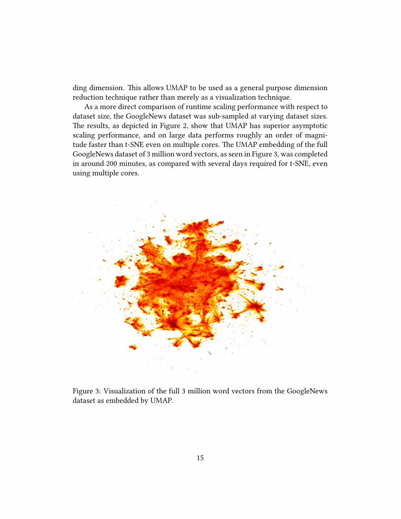
As a more direct comparison of runtime scaling performance with respect todataset size, the GoogleNews dataset was sub-sampled at varying dataset sizes.�e results, as depicted in Figure 2, show that UMAP has superior asymptoticscaling performance, and on large data performs roughly an order of magni-tude faster than t-SNE even on multiple cores. �e UMAP embedding of the fullGoogleNews dataset of 3 million word vectors, as seen in Figure 3, was completedin around 200 minutes, as compared with several days required for t-SNE, evenusing multiple cores.

Figure 3: Visualization of the full 3 million word vectors from the GoogleNewsdataset as embedded by UMAP.

15

4 ConclusionsWe have developed a general purpose dimension reduction technique that isgrounded in strong mathematical foundations. �e algorithm is demonstrablyfaster than t-SNE and provides be�er scaling. �is allows us to generate highquality embeddings of larger data sets than had been previously a�ainable.

References[1] Mikhail Belkin and Partha Niyogi. Laplacian eigenmaps and spectral tech-

niques for embedding and clustering. In Advances in neural informationprocessing systems, pages 585–591, 2002.

[2] Mikhail Belkin and Partha Niyogi. Laplacian eigenmaps for dimensionalityreduction and data representation. Neural computation, 15(6):1373–1396,2003.

[3] Gunnar Carlsson and Facundo Memoli. Classifying clustering schemes.Foundations of Computational Mathematics, 13(2):221–252, 2013.

[4] Ronald R Coifman and Stephane Lafon. Di�usion maps. Applied and com-putational harmonic analysis, 21(1):5–30, 2006.

[5] Wei Dong, Charikar Moses, and Kai Li. E�cient k-nearest neighbor graphconstruction for generic similarity measures. In Proceedings of the 20th In-ternational Conference on World Wide Web, WWW ’11, pages 577–586, NewYork, NY, USA, 2011. ACM.

[6] Greg Friedman et al. Survey article: an elementary illustrated introductionto simplicial sets. Rocky Mountain Journal of Mathematics, 42(2):353–423,2012.

[7] Paul G Goerss and John F Jardine. Simplicial homotopy theory. SpringerScience & Business Media, 2009.

[8] Harold Hotelling. Analysis of a complex of statistical variables into princi-pal components. Journal of educational psychology, 24(6):417, 1933.

[9] J. B. Kruskal. Multidimensional scaling by optimizing goodness of �t to anonmetric hypothesis. Psychometrika, 29(1):1–27, Mar 1964.

16

[10] Siu Kwan Lam, Antoine Pitrou, and Stanley Seibert. Numba: A llvm-basedpython jit compiler. In Proceedings of the Second Workshop on the LLVMCompiler Infrastructure in HPC, LLVM ’15, pages 7:1–7:6, New York, NY,USA, 2015. ACM.

[11] Yann Lecun and Corinna Cortes. �e MNIST database of handwri�en digits.

[12] John A Lee, Emilie Renard, Guillaume Bernard, Pierre Dupont, and MichelVerleysen. Type 1 and 2 mixtures of kullback–leibler divergences as costfunctions in dimensionality reduction based on similarity preservation.Neurocomputing, 112:92–108, 2013.

[13] John A Lee and Michel Verleysen. Shi�-invariant similarities circumventdistance concentration in stochastic neighbor embedding and variants. Pro-cedia Computer Science, 4:538–547, 2011.

[14] M. Lichman. UCI machine learning repository, 2013.

[15] Laurens van der Maaten and Geo�rey Hinton. Visualizing data using t-sne.Journal of machine learning research, 9(Nov):2579–2605, 2008.

[16] J Peter May. Simplicial objects in algebraic topology, volume 11. Universityof Chicago Press, 1992.

[17] Tomas Mikolov, Ilya Sutskever, Kai Chen, Greg S Corrado, and Je� Dean.Distributed representations of words and phrases and their compositional-ity. In Advances in neural information processing systems, pages 3111–3119,2013.

[18] Sameer A. Nene, Shree K. Nayar, and Hiroshi Murase. Columbia objectimage library (coil-20. Technical report, 1996.

[19] Sameer A. Nene, Shree K. Nayar, and Hiroshi Murase. object image library(coil-100. Technical report, 1996.

[20] John W Sammon. A nonlinear mapping for data structure analysis. IEEETransactions on computers, 100(5):401–409, 1969.

[21] David I Spivak. Metric realization of fuzzy simplicial sets. Self publishednotes.

17

[22] Jian Tang, Jingzhou Liu, Ming Zhang, and Qiaozhu Mei. Visualizing large-scale and high-dimensional data. In Proceedings of the 25th InternationalConference on World Wide Web, pages 287–297. International World WideWeb Conferences Steering Commi�ee, 2016.

[23] Joshua B. Tenenbaum. Mapping a manifold of perceptual observations. InM. I. Jordan, M. J. Kearns, and S. A. Solla, editors, Advances in Neural Infor-mation Processing Systems 10, pages 682–688. MIT Press, 1998.

[24] Joshua B Tenenbaum, Vin De Silva, and John C Langford. A globalgeometric framework for nonlinear dimensionality reduction. science,290(5500):2319–2323, 2000.

[25] Dmitry Ulyanov. Multicore-tsne. https://github.com/DmitryUlyanov/Multicore-TSNE, 2016.

[26] Laurens Van Der Maaten. Accelerating t-sne using tree-based algorithms.Journal of machine learning research, 15(1):3221–3245, 2014.

[27] Laurens van der Maaten and Geo�rey Hinton. Visualizing data using t-SNE.Journal of Machine Learning Research, 9:2579–2605, 2008.

[28] Jarkko Venna, Jaakko Peltonen, Kristian Nybo, Helena Aidos, and SamuelKaski. Information retrieval perspective to nonlinear dimensionality re-duction for data visualization. Journal of Machine Learning Research,11(Feb):451–490, 2010.

[29] Han Xiao, Kashif Rasul, and Roland Vollgraf. Fashion-mnist: a novel imagedataset for benchmarking machine learning algorithms, 2017.

18