ultrasonic characterization of cell pellet … phd thesis 2014.pdf · 1.2 limitations of current...
TRANSCRIPT

ULTRASONIC CHARACTERIZATION OF CELL PELLET BIOPHANTOMS AND TUMORS USING QUANTITATIVE ULTRASOUND MODELS
BY
AIGUO HAN
DISSERTATION
Submitted in partial fulfillment of the requirements for the degree of Doctor of Philosophy in Electrical and Computer Engineering
in the Graduate College of the University of Illinois at Urbana-Champaign, 2014
Urbana, Illinois
Doctoral Committee: Professor William D. O’Brien, Jr., Chair
Associate Professor Michael L. Oelze Professor Michael F. Insana
Professor Jianming Jin Dr. Emilie Franceschini, Centre National de la Recherche Scientifique
ii
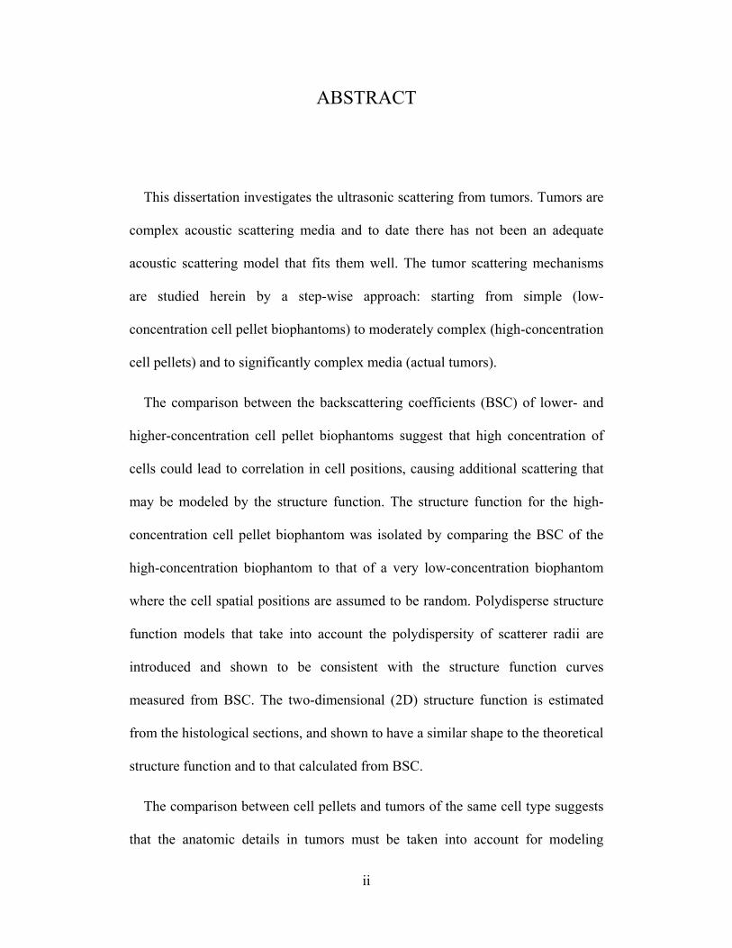
ABSTRACT
This dissertation investigates the ultrasonic scattering from tumors. Tumors are
complex acoustic scattering media and to date there has not been an adequate
acoustic scattering model that fits them well. The tumor scattering mechanisms
are studied herein by a step-wise approach: starting from simple (low-
concentration cell pellet biophantoms) to moderately complex (high-concentration
cell pellets) and to significantly complex media (actual tumors).
The comparison between the backscattering coefficients (BSC) of lower- and
higher-concentration cell pellet biophantoms suggest that high concentration of
cells could lead to correlation in cell positions, causing additional scattering that
may be modeled by the structure function. The structure function for the high-
concentration cell pellet biophantom was isolated by comparing the BSC of the
high-concentration biophantom to that of a very low-concentration biophantom
where the cell spatial positions are assumed to be random. Polydisperse structure
function models that take into account the polydispersity of scatterer radii are
introduced and shown to be consistent with the structure function curves
measured from BSC. The two-dimensional (2D) structure function is estimated
from the histological sections, and shown to have a similar shape to the theoretical
structure function and to that calculated from BSC.
The comparison between cell pellets and tumors of the same cell type suggests
that the anatomic details in tumors must be taken into account for modeling

iii
purposes, in addition to the scattering from cells. Also, histology studies suggest
that the structure functions in tumors are slightly different from those in cell
pellets: the tumor cell spatial arrangement is slightly more random compared to
cell pellets. The effect of the structure function on parameter estimation is
discussed. Further work is shown to be required for modeling the tumor structure
function.
Additionally, the comparison between different tumor types shows that
ultrasound backscattering is sensitive to unique tumor structures. The EHS tumor
has a distribution of clustered cells and shows a different BSC and structure
function pattern than the tumors that have a homogenous distribution of cells. A
scattering model is developed to detect the clustering feature.
Overall, the dissertation improves our understanding of the acoustic scattering
mechanisms in tumors, and improves the tumor scattering modeling.

iv
ACKNOWLEDGMENTS
First of all, I wish to express my grateful appreciation to my research advisor,
Dr. William D. O’Brien, Jr., for his encouragement, guidance and support
throughout this investigation. I also wish to thank my committee members, Dr.
Michael L. Oelze, Dr. Michael F. Insana, Dr. Jianming Jin and Dr. Emilie
Franceschini for their suggestions and help.
I must acknowledge Dr. Rita J. Miller, Jim Blue, Rami Abuhabsah, Jamie R.
Kelly, Matt Lee, and Ellora Sen-Gupta for their technical support in cell injection,
tumor excision, cell culture and cell pellet fabrication. Histology evaluation by
Dr. Sandhya Sarwate is also appreciated.
I am grateful to Sue Clay, Julie Ten Have, and Mary Mahaffey for their
essential administrative support, and to my co-workers from diversified
backgrounds in the Bioacoustics Research Laboratory for their valuable
discussions.
Finally, I would like to acknowledge the support and encouragement from my
family and friends throughout this challenging period.

v
TABLE OF CONTENTS
LIST OF ABBREVIATIONS .............................................................................. viii CHAPTER 1 INTRODUCTION ........................................................................... 1 1.1 Quantitative Ultrasound .................................................................................... 1 1.2 Limitations of Current QUS Models ................................................................. 2 1.3 The Proposed Study .......................................................................................... 4 CHAPTER 2 ACOUSTIC SCATTERING THEORY .......................................... 7 2.1 Backscattering Coefficient ................................................................................ 7 2.2 Uncorrelated Scatterers ..................................................................................... 8
2.2.1 Exact solutions ........................................................................................ 9 2.2.2 Approximate solutions .......................................................................... 10 2.2.3 The effect of size distribution ............................................................... 11
2.3 Correlated Scatterers ....................................................................................... 12 2.3.1 Structure function ................................................................................. 12 2.3.2 Structure function models ..................................................................... 14
2.4 Chapter Summary ........................................................................................... 17 2.5 Figures............................................................................................................. 18 CHAPTER 3 THE SCATTERING OF HIGH-CONCENTRATION BIOPHANTOMS .................................................................................................. 24 3.1 Background and Introduction ......................................................................... 24 3.2 Polydisperse Structure Functions .................................................................... 27
3.2.1 Polydisperse Model I ............................................................................ 28 3.2.2 Polydisperse Model II ........................................................................... 29
3.3 Experimental and Data Reduction Methods ................................................... 31 3.3.1 Biophantom construction ...................................................................... 31 3.3.2 Experimental setup and BSC estimation method ................................. 33 3.3.3 Histology processing ............................................................................ 35 3.3.4 B-spline fit and structure function estimation ...................................... 35
3.4 Results and Discussions .................................................................................. 37 3.4.1 BSC estimates and B-spline fit ............................................................. 37 3.4.2 Experimental and theoretical structure functions ................................. 38 3.4.3 Inverse problem .................................................................................... 40 3.4.4 Comparison to Gaussian and fluid-filled sphere BSC models ............. 42 3.4.5 The theoretical structure function for Concentration 1 ........................ 43 3.4.6 Theoretical implications of the polydisperse structure function models ............................................................................................................ 44 3.4.7 Practical usefulness of the polydisperse structure function models ..... 46
3.5 Chapter Summary ........................................................................................... 47 3.6 Figures............................................................................................................. 48 3.7 Tables .............................................................................................................. 58

vi
CHAPTER 4 BSC RESULTS FROM ANIMAL TUMORS .............................. 60 4.1 Introduction ..................................................................................................... 60 4.2 Materials and Methods .................................................................................... 62
4.2.1 Cell pellet biophantom construction ..................................................... 62 4.2.2 Animal use, cell injection and tumor sample preparation .................... 63 4.2.3 Ultrasound scanning procedure, BSC estimation method and histology processing ...................................................................................... 64
4.3 BSC and Attenuation Results and Discussion ................................................ 64 4.3.1 Tumors versus cell pellets .................................................................... 64 4.3.2 EHS tumor results ................................................................................. 70 4.3.3 Spontaneous fibroadenoma results ....................................................... 71 4.3.4 Discussion on the ex vivo condition ..................................................... 72
4.4 Chapter Summary ........................................................................................... 73 4.5 Figures............................................................................................................. 74 CHAPTER 5 ESTIMATING STRUCTURE FUNCTION FROM HISTOLOGICAL TISSUE SECTIONS .............................................................. 91 5.1 Background and Introduction ......................................................................... 91 5.2 Methods........................................................................................................... 93
5.2.1 Structure function estimation................................................................ 94 5.2.2 Pair correlation function estimation ..................................................... 95
5.3 Results and Discussions .................................................................................. 96 5.3.1 Simulations ........................................................................................... 96 5.3.2 Cell pellets ............................................................................................ 97 5.3.3 Tumors versus cell pellets .................................................................... 99 5.3.4 EHS and clustering ............................................................................. 100 5.3.5 Significance and limitations ............................................................... 101
5.4 Chapter Summary ......................................................................................... 102 5.5 Figures........................................................................................................... 103 CHAPTER 6 TUMOR SCATTERING MODELING ....................................... 120 6.1 Background and Introduction ....................................................................... 120 6.2 Effect of Structure Function on Model Parameter Estimation ...................... 122
6.2.1 Methods .............................................................................................. 122 6.2.2 Results ................................................................................................ 124 6.2.3 Discussions ......................................................................................... 124
6.3 A Model for the EHS Tumor ........................................................................ 126 6.4 Chapter Summary ......................................................................................... 127 6.5 Figures........................................................................................................... 128 CHAPTER 7 CONCLUSIONS AND FUTURE WORK .................................. 133 7.1 Structure Function Estimation and Modeling for Cell Pellets ...................... 134 7.2 The Comparison between Cell Pellets and Tumors ...................................... 134 7.3 Structure Function Estimation from Histological Sections .......................... 135 7.4 Tumor Scattering Modeling .......................................................................... 136

vii
APPENDIX A ANALYTICAL EXPRESSION OF THE STRUCTURE FUNCTION FOR POLYDISPERSE MODEL I ................................................ 138 APPENDIX B ANALYTICAL EXPRESSION OF THE STRUCTURE FUNCTION FOR POLYDISPERSE MODEL II ............................................... 142 REFERENCES ................................................................................................... 144

viii
LIST OF ABBREVIATIONS
2D Two-dimensional
2DZM Two-dimensional impedance map
3D Three-dimensional
3DZM Three-dimensional impedance map
BSC Backscattering coefficient
CHO Chinese hamster ovary
DPBS Dulbecco’s phosphate buffered saline
EAC Effective acoustic concentration
EHS Engelbreth-Holm-Swarm
ESD Effective scatterer diameter
H&E Hematoxylin and eosin
FF Fluid-filled
MAT 13762 MAT B III
NS Neyman-Scott
OZ Ornstein-Zernike
PY Percus-Yevick
QUS Quantitative ultrasound
ROI Region of interest

ix
RF Radio frequency
1
CHAPTER 1
INTRODUCTION
1.1 Quantitative Ultrasound
Diagnostic ultrasound is a significant modality in the medical imaging world. It
is safe, noninvasive, inexpensive and easily accessible. One of the most widely
used techniques in conventional ultrasound is known as B-mode imaging [1].
Acoustic reflection or scattering occur when there is an acoustic impedance
(defined as the sound speed times the mass density) contrast between two tissue
layers. B-mode images qualitatively display the brightness of the radio-frequency
(RF) echo signal, allowing for medical diagnosis. The B-mode image formation
process is simple and reliable. Medical diagnosis using B-mode imaging,
however, is often highly subjective and operator-dependent because of its
qualitative nature.
There are many approaches to constructing quantitative ultrasonic images
directly from the qualitative B-mode images. Image processing techniques such as
texture analysis has been explored for many years to extract image features such
as first- and second-order parameters including the mean, standard deviation,
entropy, and run length parameters [2]-[4]. However, these approaches only had
limited success, because the extracted quantitative parameters are system-
dependent.

2
To obtain operator- and system-independent quantitative information from the
tissue under investigation would require alternative ways of processing the RF
data. One approach is to utilize the frequency-dependent information of the RF
data and estimate the attenuation and backscatter coefficient (BSC) which are
intrinsic properties of the tissue and are not dependent on the ultrasonic system or
the operator [5], [6]. Further, acoustic scattering models that mimic tissue
anatomic structures can be fitted to the BSC versus frequency curve to estimate
acoustic properties of the scatterers, such scatterer size, shape, number density,
and acoustic impedance. The attenuation, BSC, and model-derived acoustic
parameters have been used for charactering of the eye [7], [8], prostate [9], kidney
[10], heart [11], [12], blood [13]-[16], breast [17]-[20], liver [21]-[23], cancerous
lymph nodes [24], and apoptotic cells [25], [26], and for evaluating disease
treatment [27].
1.2 Limitations of Current QUS Models
Further success of model-based QUS techniques relies on the understanding of
the tissue scattering mechanisms and the development of appropriate scattering
models that match the anatomic tissues structure. To date, the scattering
mechanisms in biological tissues have not been well understood, and the currently
available scattering models for QUS have limitations.
First, the major scattering site has not been fully identified in many cases.
Applying a simple scattering model such as the spherical Gaussian model [6] or
the fluid-fill sphere model [6] to the tissue would not yield the best result. The

3
simple model may not fit to the BSC data, and the physical/biological meanings
of model parameters are not always clear. For instance, the effective scatterer
diameter (ESD) derived from many QUS models could be interpreted as the
diameter of the cell nucleus, of the whole cell, or of other tissue structures, when
the physical sites responsible for scattering are not identified. Although the
estimated ESD may still be valuable for differentiation purposes [17], [18], the
diagnostic potential is limited and will be significantly improved if the model
parameter is correlated to a specific anatomic site or physiological state.
Second, major factors that may contribute to scattering have not been fully
explored. It has been well established in physics that the scatterer size, shape,
acoustic properties, number density, and spatial arrangement can all contribute to
scattering. Yet for tissues which factors are essential to scattering and which
factors are not has not been fully explored. This information is critical to
scattering modeling, because essentially all models have to take into account the
most important factors while ignoring the least important.
Third, many currently available models are limited to the Rayleigh region
(ka << 1, where k is the wave number and a is the scatterer size). Although the
low-frequency condition is satisfied for current clinical systems that operated in
frequencies lower than 20 MHz, models that deal with higher frequencies are
required with the emergence of high-frequency (>20 MHz) ultrasound [28]. In
fact, studying the scattering at higher frequencies will help to understand the
scattering mechanisms as well. Characterizing tissues at high frequency may yield

4
tissue property information that cannot otherwise be extracted from low-
frequency signals.
1.3 The Proposed Study
The purpose of this dissertation is to improve our understanding of the
scattering process in tissues, and eventually develop more accurate scattering
models. Biological tissues are diverse and complex. This dissertation is focused
on mammary tumors. Tumors are complex scattering media and to date there has
not been an adequate scattering model that fits it well. Studying the scattering of
tumors has medical significance: inexpensive and non-invasive tools are needed
for tumor diagnosis, and QUS has the potential to provide such a tool to diagnose
and classify tumors with high sensitivity and specificity.
There are several approaches to understanding tissue scattering. The three-
dimensional acoustic impedance map (3DZM) [29]-[31] has been used to identify
the scattering site. The 3DZMs were created by aligning serial photomicrographs
of stained histologic tumor sections. Acoustic impedance values were assigned to
the different stained colors. Another approach is to measure acoustic properties on
various tissue/cell components. For instance, the sound speed of isolated nuclei
and whole cells has been measured to study if the nucleus or the whole cell is the
scattering site [32]. Furthermore, simulations have been applied to study the
scattering process. Vlad et al. [33] performed two-dimensional simulations to
study how the cellular size variance influences ultrasound backscatter. Saha et al.
[34] performed a three-dimensional simulation to produce BSC from red blood

5
clusters, where the red blood cells in a cluster were stacked following the
hexagonal close packing structure. More complex studies include three-
dimensional simulation of the scattering for both longitudinal and shear waves
[35].
The cell pellet technique is another approach to understanding tissue scattering.
It has been demonstrated that a model termed the concentric-sphere model that
matches the geometry of a eukaryotic cell is accurate for low-concentration cell
pellet biophantoms. The biophantoms consist of live cells embedded in a plasma-
thrombin supportive background [36]. The BSC increases linearly with cell
concentration. The follow-up study [37] showed that the linear relationship
between BSC and cell concentration does not hold when the concentration is high.
Based on the cell pellet technique, in this dissertation we will use a step-wise
approach to systematically studying the scattering from tumors, i.e., to dissect the
scattering by analyzing at one time each factor that may significantly contribute to
scattering. To that end, we will compare the scattering from simple media (low
concentrations of cells), moderately complex media (high concentrations of cells),
and significantly complex media (actual tissue/tumors). The study of low-
concentration cells [36] already addressed the problem of what is responsible for
scattering from low-concentration cell pellet biophantoms. The comparison of
various concentrations may give insight into the effect of concentration on
scattering: cell concentration could affect the spatial distribution of cells. The
comparison between cells and actual tissue/tumors may demonstrate what is
unique in a specific tissue that contributes to scattering. The overall hypothesis is

6
that the scattering from tumors is dependent on three aspects: the shape and
acoustic properties of tumor cells, the spatial organization of tumor cells, and the
unique anatomic structure of each tumor type. The comparison among different
degrees of scattering media complexity can test the overall hypothesis, and lead to
improved modeling.
The overall experimental approach is to construct a variety of samples, scan the
samples using high-frequency ultrasound transducers (10 – 105 MHz), fix the
samples for further histology analysis, estimate the attenuation and BSC from the
RF data, compare the BSC of different samples, study the histological slides, and
develop and test scattering models.
The dissertation is organized as follows: Chapter 2 introduces basic scattering
theory and reviews acoustic scattering models applied to biological media.
Chapter 3 compares the scattering from low- and high-concentration cell pellet
biophantoms, and develops polydisperse structure function models to address the
effect of cell spatial distribution. Chapter 4 presents the BSC results of various
tumor types, compares the tumor BSC to the cell pellet BSC when such a
comparison is possible, and shows how unique tumor structures can affect
scattering. Chapter 5 introduces a histology-based method for estimating the
structure function, which provides independent evidence supporting the analytical
structure functions developed in Chapter 3, and provides guidelines for
developing scattering models for tumors. Chapter 6 addresses the issue of how to
develop scattering models that take into account unique tumor structures.

7
CHAPTER 2
ACOUSTIC SCATTERING THEORY
This chapter reviews the acoustic scattering theories related to soft biological
tissues. The aim is to predict the backscattering coefficient (BSC). The scatterers
are assumed to be discrete particles. Concepts of form factor and structure
function are introduced. The effect of scatterer size polydispersity is also
discussed.
2.1 Backscattering Coefficient
Consider a plane wave of unit amplitude incident on a scattering volume V that
contains N discrete scatterers. The total scattered field far from the scattering
volume behaves as a spherical wave (Equation (4) of [6]):
1
( ) ( ) j
ikr Ni
s jj
ep e
R
K rr K , (2.1)
where r is the observation position with respect to the origin, R r , jr is the
position of the jth scatterer, k is the propagation constant ( /k c where is
the angular frequency and c is the propagation speed). The factor ( )j K is the
scattering amplitude of the jth scatterer and describes the spatial frequency
Portions of this chapter are adapted from A. Han and W. D. O’Brien, Jr., “Structure function for high-concentration biophantoms of polydisperse scatterer sizes,” IEEE Trans. Ultrason. Ferroelectr. Freq. Control, accepted for publication, 2014. Used with permission.

8
dependence of the scattered pressure; j is a function of the scattering vector K
whose magnitude is given by 2 sin( / 2)k K , where is the scattering angle
( for backscattering). j is dependent on the scatterer size, shape and
acoustic properties.
The differential cross section per unit volume d (i.e., the power scattered into
a unit solid angle observed far from the scattering volume divided by the product
of the incident intensity and the scattering volume) may be expressed as
22
10
1( ) ( ) j
Nis
d jj
R Ie
VI V
K rK K , (2.2)
where sI and 0I denote the scattering intensity and incident intensity,
respectively, and 2 represents the squared modulus of the quantity.
BSC is defined as the differential cross section per unit volume to
backscattering direction ( 2kK ). The frequency-dependent BSC is an intrinsic
property of tissue, describes how effectively the tissue backscatters ultrasound,
and can be obtained experimentally by analyzing the RF data.
2.2 Uncorrelated Scatterers
If the scatterers are spatially uncorrelated (which often occurs when the
scattering volume contains a sparse concentration of scatterers without
clustering), the phase terms jie K r in Equation (2.2) may be assumed to be

9
uncorrelated. The differential cross section per unit volume for this case is
denoted as ,d incoherent , and may be expressed as
2
,1
1( ) ( )
N
d incoherent jjV
K K , (2.3)
which becomes
2
1
1(2 ) (2 )
N
incoherent jj
BSC k kV
(2.4)
for backscattering.
2.2.1 Exact solutions
For a simple scatterer shape, the exact solution of the scattering amplitude
(2 )j k may be calculated precisely by solving the wave equation. Commonly
used scatterer shapes include the fluid sphere filled in fluid [38], solid cylinders
and spheres [39], and two-fluid-concentric spheres in fluid [40]. The exact
solutions have complex expressions with multiple parameters. The simplest case,
the fluid sphere in fluid, requires at least five parameters: the scatterer radius, the
speed of sound and mass density of the scatterer, and the speed of sound and mass
density of the background.
Figure 2.1 gives an example of what the BSC versus frequency curve looks like
for the fluid-filled spheres and the concentric spheres using the exact solutions.
Note that the spatial frequency k is converted to temporal frequency in MHz, and
monodisperse scatterers are assumed.

10
2.2.2 Approximate solutions
Alternatively, a simpler expression of the scattering amplitude ( )j K may be
calculated from the spatial autocorrelation function, if the scatterers have acoustic
property values (density, ρ, and compressibility, κ) very close to those of the
background medium, and Equation (2.3) becomes (Equation (12a) of [6]),
4
2 3, 02
( ) ( )16
isd incoherent
k Vn b e d
K rK r r , (2.5)
where n is the scatterer number density (i.e., average number of scatterers per unit
volume), sV is the average scatterer volume, 20 is the mean-square variation in
acoustic impedance per scatterer, and ( )b r is the spatial autocorrelation
function of the scattering volume and depends on the scatterer shape. The integral
3( ) ib e d
K rr r is the form factor, which approaches unity when the
frequency approaches zero.
For backscattering, Equation (2.5) becomes
4
202
(2 ) (2 )16
sincoherent
k VBSC k n F k
, (2.6)
where (2 )F k is the form factor. Common form factors are [6]
2
11
3 (2 )(2 )
2
j kaF k
ka
(fluid sphere) (2.7)
22 1(2 ) (2 )F k j ka (spherical shell) (2.8)

11
2 20.827
3(2 ) effk aF k e (Gaussian) (2.9)
The BSC expressions in Equations (2.6) – (2.9) have fewer parameters and
simpler forms than the exact solution does. The simpler expressions are applicable
under the condition that the acoustic property contrast is low between the scatterer
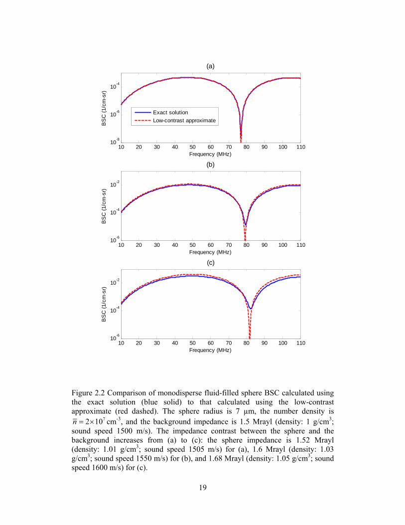
and the background. Figure 2.2 compares the fluid-filled sphere BSC calculated
using the exact solution using the Anderson model [38] to that calculated using
the low-contrast approximation using Equations (2.6) and (2.7). As the impedance
contrast between the sphere and the background increases, the approximate
solution becomes less accurate. Monodisperse spheres (radius = 7 µm) are
assumed for calculation.
2.2.3 The effect of size distribution
Typical BSC versus frequency curves have peaks and dips, and the positions of
the peaks and dips are primarily determined by the scatterer size for a given sound
speed. If the scatterers are polydisperse in size, a distribution of scatterer size will
result in smoother peaks and dips. Figure 2.3 shows the polydisperse fluid-filled
sphere BSC calculated using dist 0(2 ) (2 , ) ( ) ,BSC k BSC k x f x dx
where
dist (2 )BSC k is the BSC of the polydisperse spheres, x is the spherical radius,
( )f x is the probability density function of the spherical radius, and (2 , )BSC k x is
the BSC of monodisperse spheres that have a radius x. The quantity
(2 , )BSC k x was calculated using the exact solution (the Anderson model [38])
and the low-contrast approximation (Equations (2.6) and (2.7)), respectively. The
sphere radius is assumed to have a uniform distribution between 6 and 8 µm. The
12
size distribution makes the sharp dip (around 80 MHz) appear smoother
comparing Figure 2.2 and Figure 2.3. Further, the discrepancy between the exact
solution and the low-contrast approximate is decreased when the scatterers are
polydisperse compared to monodisperse. This result suggests that the low-contrast
approximate result may be used for polydisperse scatterers if fewer parameters are
desired for the model.
2.3 Correlated Scatterers
The spatial positions of scatterers are often correlated. The cell positions are
strongly correlated if the concentration is high. Spatial correlation in scatterer
positions can also occur at low concentrations, for example, when there is
clustering.
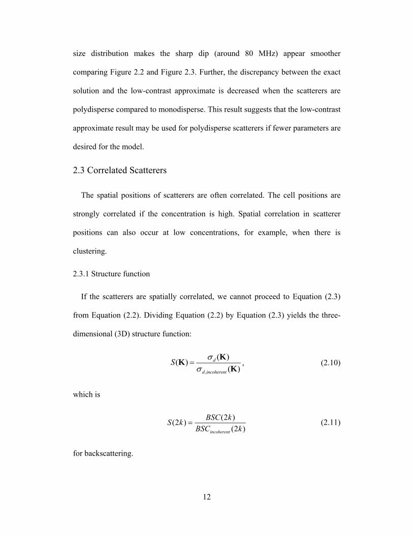
2.3.1 Structure function
If the scatterers are spatially correlated, we cannot proceed to Equation (2.3)
from Equation (2.2). Dividing Equation (2.2) by Equation (2.3) yields the three-
dimensional (3D) structure function:
,
( )( )
( )d
d incoherent
S
KK
K, (2.10)
which is
(2 )
(2 )(2 )incoherent
BSC kS k
BSC k (2.11)
for backscattering.

13
The structure function defined in Equations (2.10) and (2.11) is a quantity
describing the effect on scattering caused by the pattern of the spatial arrangement
of the scatterers. If we assume that the scattering amplitudes ( )j K are identical
for all the scatterers, Equation (2.2) may be simplified as
2
1 1
1( ) ( ) j j
N Ni i
d jj j
n e eN
K r K rK K , (2.12)
where N
nV
is the number density of the scatterers. By substituting Equation
(2.3) and Equation (2.12) into Equation (2.5), and making appropriate
simplifications, the structure function may be expressed as
1 1
1( ) j j
N Ni i
j j
S e eN
K r K rK , (2.13)
where the structure function is determined by the scatterer positions, and is not
dependent on the scattering amplitude ( )j K .
If the exact position of each scatterer is known, the structure function can be
calculated deterministically. Note that Equation (2.13) may also be expressed as
2
1
1( ) j
Ni
j
S eN
K rK , (2.14)
which means that the structure function is simply the squared modulus of the
Fourier transform of the scatterer positions. Equation (2.14) is used in Chapter 5
to estimate the structure function of a tissue from a 2D histology slide.

14
If the exact positions of the scatterers are unknown, the structure function
has to be determined statistically. In this case, the structure function can be
calculated from the statistical distribution (e.g., pair correlation function) of the
scatterer positions. Equation (2.13) is mathematically equivalent to [41]
( ) 1 ( ) 1 iS n g e d K rK r r , (2.15)
where the structure function is expressed in terms of the pair-correlation function
( )g r , a quantity related to the probability of finding two scatterers separated by
the distance r. With Equation (2.15), the structure function can be interpreted as
the 3D Fourier transform of the total correlation function ( ) ( ) 1h g r r . The
total correlation may be obtained by solving the set of equations formed by the
Ornstein-Zernike (OZ) integral equation [42] and a closure relation. The OZ
equation splits the total correlation ( )h r into the direct correlation ( )c r and the
indirect correlation by the equation 0
( ) ( ) (| ' |) (| ' |) 'h r c r n h r r c r dr
. The
closure relation couples the same quantities h and r. Depending on different
models of closure relation, the structure function will be different.
2.3.2 Structure function models
A number of structure function models have been successfully used in
ultrasonic tissue characterization, particularly in blood characterization. The
Percus-Yevick (PY) structure function [43] is typically used to model the
structure of dense medium that does not have clustering. To address the clustering
effect, the structure function derived from the Neyman-Scott (NS) point process
was used for blood characterization [44]. Additionally, a second-order Taylor

15
approximation of structure function [45] was developed to achieve a
mathematically simple expression.
A) Percus-Yevick approximation
The PY approximation is a commonly used closure relation valid for a random
distribution of non-overlapping spheres (the sphere positions are not truly random
because they are non-overlapping). With PY closure, an analytical expression of
the structure function has been obtained for backscattering [46]-[48]:
1
(2 )1 (2 )PYS k
nC k
, (2.16)
13 2 3
0
sin(4 )(2 ) 32
4
kasC k a s s s ds
kas , (2.17)
34
3
an
, 2
4
(1 2 )
(1 )
,
2
4
6 (1 / 2)
(1 )
,
2
4
(1 2 )
2(1 )
, (2.18)
where a is the sphere radius, s is a dummy variable of integration, and is the
sphere volume fraction.
Figure 2.4 shows a comparison among the PY structure functions at various
volume fractions (similar results can be found in [47] and [48]. The PY structure
function approaches unity as the concentration becomes extremely low. A peak
starts to appear around ka = 2 as the concentration increases. The peak becomes
relatively sharp as the concentration becomes considerably large. This sharp peak
is not observed from tissue data, because the scatterers in tissue are polydisperse
in nature, whereas the PY structure function given in Equations (2.16) – (2.18) is

16
only valid for identical scatterers. Structure functions that are based on the PY
closure relation but take into account the scatterer polydispersity are developed in
Chapter 3, and applied to the high-concentration cell-pellet biophantoms.
B) Neyman-Scott point process
The NS process is a random point process commonly used to model clusters of
points [44]. The NS process applied in [44] assumes that the spatial distribution of
cluster centers follows a Poison distribution, and the spheres within the cluster
follow a Gaussian distribution (more spheres in the cluster center). The resulting
structure function is given by
2 22( ) /(2 ) 1 ( 1) ka
NSS k W e , (2.19)
2c c c( / )W n n , (2.20)
1/
c
11
2fD
n , (2.21)
where nc and 2c are the mean and variance of the number of scatterers per
cluster, fD is the fractal dimension that morphologically characterizes the growth
process of the aggregates ( 3fD for compact spherical aggregates), W is the
packing factor which increases when the number of cells per aggregate grows,
and Δ is the size factor which decreases when the spatial dimension of the cluster
increases.
Figure 2.5 plots the NS structure functions calculated using four sets of
parameters. The NS structure function approaches unity when the average number

17
of scatterers per cluster is one. This observation means that the NS structure
function only models the clustering effect, but does not take into account the
concentration effect on scatterer position correlation. Therefore, it only works for
low scatterer concentrations (volume fraction less than 5%). As the number of
scatterers per cluster increases, the structure function increases in the low-
frequency range (ka < 0.5), whereas it remains unity at the high-frequency range.
C) Second-order Taylor approximation
A second-order Taylor approximation of structure function was given in [45] as
2212(2 )
5TaylorS k W D ka , (2.22)
where W is the packing factor, and D equals the aggregate radius divided by the
scatterer radius. W and D have been shown to increase during blood aggregation
[45].
Figure 2.6 plots the structure functions calculated by Equation (2.22) using four
sets of parameters picked from Table V of [45].
2.4 Chapter Summary
The scattering from soft tissue is affected not only by the properties of
individual scatterers (e.g., scatterer size, shape, acoustic impedance contrast), but
also by the scatterer position correlation. The scatterer positions can be
significantly affected by clustering, high concentration, etc. Success has been
achieved in literature using the structure function to address the scatterer position

18
correlation issue. However, limitations also exist in available structure function
models.
2.5 Figures
10 20 30 40 50 60 70 80 90 100 11010
-7
10-6
10-5
10-4
10-3
10-2
Frequency (MHz)
BS
C (
1/cm
-sr)
Concentric sphere (ain
= 4 m, aout
= 7 m)
Single fluid-filled sphere (a = 7 m)
Single fluid-filled sphere (a = 4 m)
Figure 2.1 Comparison of calculated BSC versus frequency curves for the concentric sphere model and the single fluid-filled sphere model using the exact solutions. The parameters used for the concentric sphere (blue solid) are: inner sphere radius ain = 4 µm, outer shell radius aout = 7 µm, inner sphere impedance Zin = 1.6 Mrayl (density: 1.03 g/cm3; sound speed: 1550 m/s), outer shell impedance Zout = 1.55 Mrayl (density: 1.01 g/cm3; sound speed 1535 m/s), background impedance Z0 = 1.5 Mrayl (density: 1 g/cm3; sound speed 1500 m/s), and number density 72 10n cm-3. The parameters used for the larger fluid-filled sphere (dotted magenta) are: radius a = 4 µm, sphere impedance Z = 1.55 Mrayl (density: 1.01 g/cm3; sound speed 1535 m/s), background impedance Z0 = 1.5 Mrayl (density: 1 g/cm3; sound speed 1500 m/s), and number density
72 10n cm-3. The parameters used for the smaller fluid-filled sphere (dashed red) are the same as the larger one except that the sphere radius is set to be 4 µm.
19
10 20 30 40 50 60 70 80 90 100 11010
-8
10-6
10-4
Frequency (MHz)
BS
C (
1/cm
-sr)
(a)
Exact solution
Low-contrast approximate
10 20 30 40 50 60 70 80 90 100 11010
-6
10-4
10-2
Frequency (MHz)
BS
C (
1/cm
-sr)
(b)
10 20 30 40 50 60 70 80 90 100 11010
-6
10-4
10-2
Frequency (MHz)
BS
C (
1/cm
-sr)
(c)
Figure 2.2 Comparison of monodisperse fluid-filled sphere BSC calculated using the exact solution (blue solid) to that calculated using the low-contrast approximate (red dashed). The sphere radius is 7 µm, the number density is
72 10n cm-3, and the background impedance is 1.5 Mrayl (density: 1 g/cm3; sound speed 1500 m/s). The impedance contrast between the sphere and the background increases from (a) to (c): the sphere impedance is 1.52 Mrayl (density: 1.01 g/cm3; sound speed 1505 m/s) for (a), 1.6 Mrayl (density: 1.03 g/cm3; sound speed 1550 m/s) for (b), and 1.68 Mrayl (density: 1.05 g/cm3; sound speed 1600 m/s) for (c).

20
10 20 30 40 50 60 70 80 90 100 11010
-8
10-6
10-4
Frequency (MHz)
BS
C (
1/cm
-sr)
(a)
Exact solution
Low-contrast approximate
10 20 30 40 50 60 70 80 90 100 11010
-6
10-4
10-2
Frequency (MHz)
BS
C (
1/cm
-sr)
(b)
10 20 30 40 50 60 70 80 90 100 11010
-6
10-4
10-2
Frequency (MHz)
BS
C (
1/cm
-sr)
(c)
Figure 2.3 Comparison of polydisperse fluid-filled sphere BSC calculated using the exact solution (blue solid) to that calculated using the low-contrast approximate (red dashed). The parameters are the same as Figure 2.2, except that the sphere radius is assumed to following a uniform distribution between 6 and 8 µm.

21
Figure 2.4 Comparison among PY structure functions at five different volume fractions: 1%, 10%, 50%, 60%, and 74%, computed using Equations (2.16) – (2.18).

22
0 0.1 0.2 0.3 0.4 0.5 0.6 0.7 0.8 0.9 10
2
4
6
8
10
12
14
16
ka
S(2
k)
nc = 1, c
2 = 0
nc = 5, c
2 = 4
nc = 15, c
2 = 4
nc = 15, c
2 = 40
Figure 2.5 Comparison among NS structure functions for four parameter sets: (a) nc = 1, 2
c = 0, (b) nc = 5, 2c = 4, (c) nc = 15, 2
c = 4, and (d) nc = 5, 2c = 40,
using Equations (2.19) – (2.21). fD is assumed to be 3 for all four curves.

23
0 0.1 0.2 0.3 0.4 0.5 0.6 0.7 0.8 0.9 1-70
-60
-50
-40
-30
-20
-10
0
10
ka
S(2
k)
W = 1.4, D = 2.4
W = 6.8, D = 5.3
W = 0.5, D = 1.1
W = 0.2, D = 0.7
Figure 2.6 Comparison among structure functions calculated by second-order Taylor approximation using four parameter sets: (a) W = 1.4, D = 2.4, (b) W = 6.8, D = 5.3, (c) W = 0.5, D = 1.1, and (d) W = 0.2, D = 0.7.

24
CHAPTER 3
THE SCATTERING OF HIGH-CONCENTRATION BIOPHANTOMS
This chapter addresses the problem of dense media scattering using structure
functions. The effect of scatterer polydispersity on the structure functions is
investigated. Structure function models based on polydisperse scatterers are
theoretically developed and experimentally evaluated against the structure
functions obtained from cell pellet biophantoms.
3.1 Background and Introduction
A previous study [36] demonstrated that a concentric-sphere model that
matches the geometry of a eukaryotic cell is accurate for low-concentration cell
pellet biophantoms that consist of live cells embedded in a plasma-thrombin
supportive background. The study [36] also showed that the ultrasonic backscatter
coefficient (BSC) increases linearly with cell concentration. The follow-up study
[37] showed that the linear relationship between BSC and cell concentration does
not hold when the concentration is high. There was no adequate model that could
apply to the high-concentration cell pellet biophantoms. In the meantime,
This chapter is adapted from A. Han and W. D. O’Brien, Jr., “Structure function for high-concentration biophantoms of polydisperse scatterer sizes,” IEEE Trans. Ultrason. Ferroelectr. Freq. Control, accepted for publication, 2014. Used with permission.
25
modeling such dense media is of practical significance because the cell
concentration is high in real tissues such as mammary tumors.
Given the acoustic scattering theory reviewed in Chapter 2, it is hypothesized
that higher concentration causes stronger spatial correlation in the cell positions.
The structure function could be useful to address this problem.
The structure function has been applied in a number of areas of ultrasonic
scattering. To give a more comprehensive review than what have been mentioned
in Chapter 2, the concept of structure function was introduced for the first time by
Twersky [41], [49] to model ultrasonic scattering. The structure function was used
to model the differential cross section per unit volume for a random distribution
of identical scatterers [41] and for a mixture of similarly shaped but differently
sized particles [49]. In the field of QUS techniques for tissue characterization,
Franceschini et al. [15] recommended a method to model the scattering from
densely packed cells in tumors using BSC models that take into account the
structure function. They performed experiments on concentrated tissue-mimicking
phantoms and showed the superiority of the BSC models that take into account
the structure function in comparison with other classical BSC models that do not
account for the structure function. Vlad et al. [33] performed two-dimensional
simulations to study the difference in the backscattering coefficient between the
particle distribution with uniform and heterogeneous sizes. They also made a
comparison with the Percus-Yevick packing factor – the low-frequency limit of
the PY structure function. In [33] and another study [50], particle size variance

26
was shown to be affecting the structure function and BSC behavior in the case of
highly concentrated scattering medium.
Although structure function has seen many applications in ultrasonic scattering,
none of the available structure function models in the field of medical ultrasound
work well for high-concentration cell pellet biophantoms. Most models were
developed for specific conditions and have limitations. For example, the PY
structure function starts to show a sharp peak (Figure 2.4) when the concentration
becomes relatively high (volume fraction > 50%). Such a sharp peak is not
physically realistic. The NS model deals with clustering and does not take into
account the concentration issue. Therefore, a new structure function model is
needed.
To best model the structure function and demonstrate its effect, it is desirable to
separate the effect of the form factor. Therefore, instead of modeling the BSC that
is affected by both the structure function and the form factor, we focus only on
modeling the structure function in this chapter.
Specifically, we will develop analytical structure function models for randomly
distributed scatterers that are polydisperse in size, and evaluate the models against
the cell pellet biophantoms both forwardly and inversely. More specifically, we
will estimate the BSCs of cell pellet biophantoms at two concentrations, a very
low concentration where the cells are randomly distributed, and a very high
concentration where the cells are closely packed to mimic the condition of a
tumor. The structure function that is related to the spatial distribution of cell
positions will be isolated by comparing the BSCs of the two concentrations. The
27
theoretical structure function will be calculated from three models and compared
to the experimentally estimated values. The inverse problem will also be explored
to generate cell size estimates. Three distinct cell lines will be studied to
demonstrate repeatability.
A number of advantages exist in the models developed and the approach used
in this chapter: (1) By studying only the structure function rather than the BSC,
the effect of spatial scatterer position correlation on scattering is separated and
thus can be better studied. (2) The developed structure function models will be
able to elucidate the effects of scatterer size distribution on scattering. For
instance, the polydisperse structure function models suggest that the size
distribution could affect the BSC by affecting not only the incoherent scattering
component (which is well established), but also the structure function. (3) The
models have minimal dependence on the form factor, which is a significant
advantage because identifying the best form factor for a tissue is challenging. (4)
The models are in analytical forms and have a limited number of variables, which
makes the inverse problem easier to solve. (5) The study is strengthened by
evaluating the models in a forward manner using high-frequency (the center of the
frequency band is around ka = 2) experimental data from biophantoms that
mimics tumors.
3.2 Polydisperse Structure Functions
We will start with the PY structure function model introduced in Chapter 2.
The sharp peak (Figure 2.4) occurs in the structure function curve at high

28
concentration because the scatterers were assumed to be identical spheres when
Equations (2.16) – (2.18) were derived. Intuitively, identical spheres could lead to
a spatial arrangement that is more periodic than polydisperse spheres would under
the high-concentration situation. Taking into account the polydispersity in sphere
size could reduce the sharp peak in the PY structure function. Two polydisperse
structure function models are developed to achieve this goal. For comparison
purposes, the PY structure function introduced in Chapter 2 is also called the
Monodisperse Model in this chapter, and will be compared to the polydisperse
models.
3.2.1 Polydisperse Model I
In this model, the scatterers are assumed to be non-overlapping spheres that are
polydisperse in size but monodisperse in scattering amplitudes ( )j K . Note that
the assumption of monodisperse scattering amplitude is unrealistic if the system is
polydisperse in size, because the scattering amplitude is a function of scatterer
size. We make the monodisperse scattering amplitude assumption simply as a
mathematical approximation such that Equation (2.15) will still hold, and the
structure function will be determined solely by the pair-correlation function. As
such, the structure function may be written in terms of partial structure
functions (2 )ijH k as given by Blum and Stell [51] using PY closure as in [52]
0 0
(2 ) 1 (2 ) ( ) ( )ij i j i jS k n H k f x f x dx dx
, (3.1)
where ( )f x is the probability density function of the sphere radius, x.

29
The structure function has an analytical expression following Equation (3.1) if
the sphere size follows a Γ (Schulz) distribution with a probability density
function [52]
1 ( 1)1 1
( ) , 0,1, 2,...!
z z xz a
z
zf x x e z
z a
, (3.2)
where a is the mean of the radius, and z is the Schulz width factor which measures
the width of the distribution (a greater z representing a narrower distribution). The
Γ distribution has been widely used to model polydisperse biological systems, and
is an ideal distribution to use for cells.
The analytical expression of the structure function for Polydisperse Model I is
listed in Appendix A. The structure function is expressed as a function of mean
sphere radius a, Schulz width factor z, wave number k, and sphere volume
fraction η. The structure functions at various Schulz width factors are shown in
Figure 3.1. When z , the Polydisperse Model I yields the same result as that
of Monodisperse Model, which could serve as a code sanity check. As the
polydispersity of sphere radius increases (i.e., z decreases), the peak of the
structure function curve reduces accordingly.
3.2.2 Polydisperse Model II
Polydisperse Model I does show decreased peak values compared to the
Monodisperse Model for high concentrations as expected. However, an unrealistic
assumption was made during the development of Polydisperse Model I: the
scatterers were assumed to be polydisperse in size but monodisperse in scattering
amplitudes ( ).j K This assumption allows for convenient mathematical

30
approximation to be made. To investigate if the assumption is reasonable,
Polydisperse Model II is developed and compared to Polydisperse Model I.
For Polydisperse Model II, the scatterers are assumed to be non-overlapping
spheres that are polydisperse in both size and scattering amplitude, and the sphere
size is assumed to follow a Γ distribution. As a result of the polydispersity in
scattering amplitude, the scattering amplitude cannot be factored out in Equation
(2.2). Therefore, Equations (2.13) and (2.15) are not valid any more. To derive the
structure function expression for this case, we express the BSC as
2
0
0 0
(2 ) | (2 ) | ( )
(2 ) (2 ) (2 ) ( ) ( )
j j j
i j ij i j i j
BSC k n k f x dx
n k k H k f x f x dx dx
. (3.3)
Equation (3.3) is a modification of Equation (1) of [53]. Similar expressions may
also be found in [49]. The first integral 2
0| (2 ) | ( )j j jn k f x dx
of Equation (3.3)
represents the quantity (2 )incoherentBSC k . The second integral of Equation (3.3)
represents the excess scattering caused by the spatial correlation in scatterer
positions. Substituting Equation (3.3) into Equation (2.11) yields the structure
function for Polydisperse Model II:
0 0
2
0
(2 ) (2 ) (2 ) ( ) ( )(2 ) 1
| (2 ) | ( )
i j ij i j i j
j j j
k k H k f x f x dx dxS k
k f x dx
. (3.4)
This structure function is dependent on the scattering amplitude (2 )j k .
Therefore, a specific form of scattering amplitude is needed to evaluate Equation
(3.4). The scattering amplitude that is used herein is derived from the fluid-filled

31
sphere form factor in Equation (2.7) for which the integrals in Equation (3.4) have
analytical expressions. The resulting expression for the structure function is listed
in Appendix B. The structure function is expressed as a function of the mean
sphere radius a, Schulz width factor z, wave number k, and sphere volume
fraction η. The structure functions for Polydisperse Model I and Polydisperse
Model II are compared at various degrees of polydispersity (Figure 3.2). The peak
at around ka = 2 in the structure function curve is lower for Polydisperse Model II
than for Polydisperse Model I when the scatterers are polydisperse (Figure 3.2(a)-
(c)), suggesting that the monodisperse scattering amplitude assumption made for
Monodisperse Model I does affect the structure function result. However, the
discrepancy between the two polydisperse models tends to be reduced as the
polydispersity is reduced. As a code sanity check, Polydisperse Model I and
Polydisperse Model II generate identical results when the scatterers are essentially
monodisperse (Figure 3.2(d)).
3.3 Experimental and Data Reduction Methods
3.3.1 Biophantom construction
The cell pellet biophantoms were composed of a known number of cells clotted
in a mixture of bovine plasma (Sigma-Aldrich, St. Louis, MO) and bovine
thrombin (Sigma-Aldrich, St. Louis, MO). Three cell lines, Chinese hamster
ovary [CHO, American Type Culture Collection (ATCC) #CCL-61, Manassas,
VA], 13762 MAT B III (MAT, ATCC #CRL-1666) and 4T1 (ATCC #CRL-
2539), were used to create the cell pellet biophantoms. The three cell lines were
chosen because: (1) they represent normal and tumor cell lines (normal cells:

32
CHO, tumor cells: MAT and 4T1), and (2) they represent different cell sizes (see
Figure 3.3 for measured cell radius histograms and the corresponding Schulz
distribution fit). Two cell concentrations (Table 3.1) were realized for each cell
line, with each concentration having two to three independent replicates of
biophantoms.
The detailed procedure of constructing cell pellet biophantoms is as follows.
The cells were cultured in an ATCC-recommended medium along with 8.98% of
fetal bovine or calf serum (Hyclone Laboratories, Logan, UT) and 1.26% of
antibiotic (Hyclone Laboratories, Logan, UT). A Reichert Bright-Line®
hemacytometer (Hausser Scientific, Buffalo, NY) was used to count viable cells
to yield the number of cells per known volume. Equal volumes of the dye Trypan
Blue (Hyclone Laboratories, Logan, UT) and cell suspension were gently mixed
by pipetting and then added to the counting chambers of the hemacytometer.
Trypan Blue was used to differentiate nonviable cells (stained as blue cells) from
viable cells (displayed as bright cells). At this point, the cells had an average of
over 90% viability. A known number of viable cells was placed in a 50-mL
conical centrifuge tube (Corning® Incorporated, Corning, NY), and spun in a 4 °C
centrifuge at 2500 rpm for 10 min, and the supernatant was removed. Then, 90 µL
of bovine plasma were added to the cell sediment in the centrifuge tube, which
was then vortexed. Next, 60 µL of bovine thrombin were added, and the mixture
was lightly agitated to coagulate and form a biophantom. The biophantom was
transferred onto a planar Plexiglas® plate, and submerged in Dulbecco’s

33
Phosphate Buffered Saline (DPBS) (Sigma-Aldrich, St. Louis, MO) for ultrasonic
scanning.
3.3.2 Experimental setup and BSC estimation method
The biophantoms were ultrasonically scanned using three single-element,
weakly focused transducers (20-MHz transducer IS2002HR, from Valpey Fisher
Cooperation, Hopkinton, MA; 40- and 80-MHz transducers from NIH High-
frequency Transducer Resource Center, University of Southern California, Los
Angeles, CA; see Table 3.2). The total frequency range covered was 11 to 105
MHz.
The transducers were interfaced with a UTEX UT340 pulser/receiver (UTEX
Scientific Instruments Inc., Mississauga, ON, Canada) that operated in the pitch-
catch mode. A 50DR-001 BNC attenuator (JFW Industries Inc., Indianapolis, IN)
was connected to the pulser to attenuate the driving pulse to avoid transducer
saturation. An RDX-6 diplexer (Ritec Inc., Warwick, RI) was used to separate the
transmitted and received signals because only the transmitted signal needed to be
attenuated. The received RF signals were acquired using a 10-bit Agilent
U1065A-002 A/D card (Agilent Technologies, Santa Clara, CA) set to sample at 1
GHz. The transducers were moved using a precision motions control system
(Daedal Parker Hannifin Corporation, Irwin, PA) that has a linear spatial accuracy
of 1 µm. The biophantoms were placed on the Plexiglas® plate during ultrasound
scans. The scans were performed in a small tank filled with DPBS at room
temperature (Figure 3.4).

34
Attenuation and BSC measurements were performed for each sample. The
attenuation was determined to allow for attenuation compensation during the BSC
estimation process. An insertion-loss broadband technique [54] was used to
estimate the attenuation. The insertion loss was determined by comparing the
power spectra of the echoes reflected off the top surface of the Plexiglas® with
and without the sample being inserted in the ultrasound path. The transducer
focus was positioned at the Plexiglas® surface when the signal was being
recorded. The effect of DPBS attenuation was compensated for when the
biophantom attenuation was estimated from the insertion loss. The attenuation
(dB/cm) of a sample was generated by averaging the attenuation obtained from 36
independent locations laterally across the sample.
The BSC scanning procedure started with acquiring the reference signals from
the DPBS-Plexiglas® interface whose pressure reflection coefficient at room
temperature is known (= 0.37). The reference signals were acquired at the set of
axial positions that covered the –6 dB depth of focus with a step size of a half
wavelength. Next, a raster scan on the biophantom sample was performed with a
lateral step size of one beam width. The transducer focus was positioned in the
sample during the scan. The scan covered a sufficient length both axially and
laterally to make sure that a sufficient number of regions of interest (ROIs) could
be acquired and processed. Eleven equally spaced slices were imaged for each
sample, and the number of A-lines per sample varied depending on the transducer
frequency and sample size. The BSC was estimated from the RF data using a
planar reference method [55] to remove equipment-dependent effects. To generate

35
a BSC versus frequency curve for a sample scanned by a single transducer, (i) a
BSC estimate was made for each ROI based on the gated RF echo data from that
ROI, (ii) a mean BSC was estimated for each of the 11 slices by averaging the
BSCs from all the ROIs within that slice, and (iii) the 11 mean BSCs were
averaged.
3.3.3 Histology processing
Immediately after scanning, the sample was placed into a histology processing
cassette and fixed by immersion in 10% neutral-buffered formalin (pH 7.2) for a
minimum of 12 h for histopathologic processing. The sample was then embedded
in paraffin, sectioned, mounted on glass slides and stained with hematoxylin and
eosin (H&E) for further evaluation by light microscopy (Olympus BX–51,
Optical Analysis Corporation, Nashua, NH, USA).
3.3.4 B-spline fit and structure function estimation
Two concentrations (Table 3.1) were studied for each cell line: the higher
concentration was chosen to be as high as possible to mimic the cell concentration
in tumors, and the lower concentration was chosen to be sufficiently low such that
the structure function can be assumed to be unity, while still high enough to
ensure sufficient signal-to-noise ratio in the backscatter data. Based on these
conditions, the structure function for the higher concentration may be obtained
experimentally by
( )
( )( )
L H
H L
n BSC fS f
n BSC f , (3.5)

36
where Ln and Hn represent the number density for the lower and the higher
concentrations, respectively, ( )LBSC f and ( )HBSC f represent the BSC for the
lower and the higher concentrations, respectively.
There were a number of BSC versus frequency curves obtained from multiple
transducers and multiple realizations for each concentration of each cell line. A B-
spline fit was performed on these curves to generate a single fitted curve that
covered the entire frequency range (11 – 105 MHz) for a concentration of a cell
line. The fitted BSC values were used for structure function estimation using
Equation (3.5).
The B-spline is a commonly used smoothing spline for large data sets. The
advantage of a smoothing spline is that the resulting curve is not required to pass
through each data point. The resulting B-spline curve is a linear combination of M
B-spline basis functions, where M is the degrees of freedom, and the B-spline
basis functions are spaced at different locations to provide local shape control. In
this dissertation, we fit cubic B-splines with five degrees of freedom, giving us
five B-spline basis curves at five equally spaced locations in the frequency range.
The best-fit B-spline is then a linear combination of five B-spline basis functions:
5
1
( ) ( )i ii
fbs b f
, (3.6)
where ( )ib f is the ith B-spline basis function, and i is the corresponding
coefficient of each basis function to control the shape locally. The calculation of

37
( )ib f and the least square estimation of i are performed using custom programs
developed in MATLAB® (The Mathworks Inc., Natick, MA).
3.4 Results and Discussions
3.4.1 BSC estimates and B-spline fit
The attenuation-compensated BSC estimates for the biophantoms are shown in
Figure 3.5 for each cell line. The BSC curves of all realizations were plotted to
show the degree of measurement uncertainty and/or the uncertainty in
concentration control. Overall, multiple realizations had consistent BSC results.
The BSC behaviors in Figure 3.5 reveal significant information about the
structure function. The BSC shape is significantly different between the lower and
higher concentrations for all three cell lines. This observation confirms that it is
necessary to consider the structure function for the higher concentration
condition. The BSC magnitude appears to be similar between the lower and
higher concentrations at lower frequencies (f < 30 MHz), whereas the difference
in BSC magnitudes of the two concentrations start to increase at higher
frequencies (f ~ 60 MHz). A physical interpretation of this behavior is that the
effect of cell position correlation on scattering for the high-concentration case is
destructive at frequencies lower than 30 MHz, and is constructive (or less
destructive) at around 60 MHz. This interpretation is consistent with the shape of
the theoretical structure functions presented in Figures 2.4, 3.1, and 3.2: the
structure functions are lower than unity at lower ka values, and are peaking at
around ka = 2. Furthermore, a peak at around 60 MHz, and a dip at around 90

38
MHz are observed for every BSC curve. The peak and dip behavior for the lower-
concentration case is explained by form factors (e.g., fluid-filled sphere,
concentric spheres) that match the geometry and acoustic impedance distribution
of individual cells. The peak for the higher concentration is sharper compared
with the lower concentration. None of the commonly used form factors for soft
materials could yield such a sharp peak, indicating that other factors such as the
structure function might contribute to the sharp peak.
3.4.2 Experimental and theoretical structure functions
The experimental structure function (Figure 3.6) for Concentration 2 (see Table
3.1) was determined using Equation (3.5) assuming the structure function was
unity for Concentration 1 as discussed in details in Section 3.4.5. The theoretical
structure functions (including the two polydisperse models developed in this
chapter and the Monodisperse Model (PY) reviewed in Chapter 2, Figure 3.6) for
Concentration 2 were calculated using the three structure function models. For the
theoretical calculation, the volume fraction was assumed to be 74% for
Concentration 2. The values of parameters a and z used for theoretical calculation
were the same as the Schulz distribution fit results presented in Figure 3.3. To
convert from k to f, a propagation speed of 1540 m/s was assumed throughout this
chapter.
Figure 3.6 shows that the theoretical structure functions from the three models
have a peak-dip pattern consistent with that of the experimental structure function.
The positions of the peaks and dips are well aligned between the theoretical and
experimental curves. However, the exact magnitude of the major peak varies

39
between the theoretical and experimental curves. The Monodisperse Model shows
the highest peak, which extends well above 7 and is clipped in Figure 3.6.
Polydisperse Model I shows a lower peak, and Polydisperse Model II shows the
lowest peak among all three models. Relative to the magnitude of the peak,
Polydisperse Model II has the best agreement to the experimental curve, and
therefore seems to be the most accurate model out of the three.
Although the theoretical curves of the two polydisperse models show
agreement with the experimental curves, the agreement is not perfect. A perfect
agreement is not expected, because the scattering of cells is so complex that many
factors could contribute to scattering. The structure function only models one
factor, the spatial correlation of cell positions, and shows that this factor is
important. Other factors, such as multiple scattering, might explain in general why
the polydisperse models do not perfectly agree with experimental data. That being
said, we try herein to explain, within the framework of structure function, a
number of observed discrepancies between the models and the experimental data.
The polydisperse models seem to work better for CHO and MAT than for 4T1.
This observation might be attributed to the fact that 4T1 has the highest degree of
polydispersity among all the three cell lines. A higher degree of polydispersity
leads to a smoother peak in the structure function. A smooth peak is easier to be
shifted due to measurement errors than a sharp peak. Another noticeable
difference between the theoretical and experimental curves is that the peak of the
theoretical curves is higher than that of the experimental curves. There could be a
number of explanations for this difference. We might have underestimated the

40
polydispersity of cells. We have considered only the polydispersity in cell size,
but not the polydispersity in cell shape. Experimental errors might as well
contribute to the difference. For instance, if the attenuation was underestimated
for the higher concentration, then the BSC might be underestimated consequently,
resulting in an underestimated experimental structure function. Also, the volume
fraction of 74% might have uncertainty. If the actual volume fraction was slightly
deviated from 74%, then the theoretical structure function in Figure 3.6 would be
slightly different as well.
3.4.3 Inverse problem
The usefulness of Polydisperse Models I and II is demonstrated herein via
solving the inverse problem: estimating the mean radius from experimental
structure functions.
The mean radius a and the Schulz width factor z were the unknowns in the
inverse problem. The volume fraction was assumed to be known a priori
(η = 74%). The two unknowns were estimated by fitting the theoretical structure
function SFtheo(f) to the experimental structure function SFexp(f). Specifically, we
perform an exhaustive search procedure for values of
( , ) [4 m,12 m] [5,100]a z to minimize the cost function:
2theo exp( , ) || ( ) ( ) ||i i
i
C a z SF f SF f (3.7)
over the frequency range 11–105 MHz.
41
The results of the search show that a unique global minimum always exists for
the CHO, MAT, and 4T1 cell pellets for Polydisperse Model I and Polydisperse
Model II. A typical logarithm of the cost function ( , )C a z is shown in Figure
3.7(a). The mean radius estimates and the Schulz width factor estimates are
shown in Figure 3.7(b) and Figure 3.7(c), respectively. Overall Polydisperse
Models I and II yield relatively accurate mean radius estimates, with a maximum
percentage error of 13.5% for Polydisperse Model I and 6.7% for Polydisperse
Model II for all three cell lines evaluated. As expected, Polydisperse Model II
provides slightly better size estimates than does Polydisperse Model I. The Schulz
width factor estimates are not as accurate as the mean radius estimates. Both
polydisperse models underestimate the Schulz width factor, i.e., overestimate the
degree of polydispersity in cell size, possibly because the polydispersity in cell
shape might also contribute to scattering and could decrease the estimated Schulz
width factor value. It is not surprising that Polydisperse Model II yields a better
Schulz width factor estimate than does Polydisperse Model I, because
Polydisperse Model II takes into account the polydispersity in scattering
amplitude to some extent, whereas Polydisperse Model I does not. Although the
Schulz width factor z is underestimated by the models, the estimated z values are
accurate in relative terms: 4T1 has the lowest z values, both measured and
estimated, and MAT has the highest z values, both measured and estimated.
The fitted structure function curves (Figure 3.8) show good agreement with the
experimental curves in terms of peak positions. This observation is consistent
with the relatively good accuracy in size estimates, because the position of the

42
peak is mainly determined by the cell size. Polydisperse Model II appears to have
better-fitted curves than Polydisperse Model I in terms of agreement in the peak
magnitude (Figure 3.8). This observation might explain why Polydisperse Model
II has better Schulz width factor estimates, because the peak magnitude is
presumably related to the Schulz width factor more than to the mean radius.
3.4.4 Comparison to Gaussian and fluid-filled sphere BSC models
To test whether fitting the structure function curves could yield better mean cell
radius than fitting BSC curves, we fit two commonly used BSC models, the
spherical Gaussian (Equations (2.6) and (2.9)) and the fluid-filled sphere model
(Equations (2.6) and (2.7)), to the high-concentration BSC curves presented in
Figure 3.5. Both BSC models take into account only the geometry and acoustic
impedance profile of the cells, but not the spatial correlation of cell positions. The
detailed estimation procedure can be found in [18]. The estimated effective
scatterer radius from the two BSC models is compared with the estimated mean
cell radius from the two polydisperse structure function models (Figure 3.9). The
two polydisperse structure function models show advantage in terms of estimating
the cell radius. They yield relatively accurate mean cell radius estimates, whereas
the two BSC models do not. One might argue that the effective scatterer size
estimates from the two BSC models might correspond to the size of cell nucleus.
In fact, this argument pointed out a significant disadvantage of the two BSC
models: it is difficult to relate the effective scatterer size estimates to real tissue
anatomy. It is not clear if the effective scatterer size estimates relate to the cell
radius, the nucleus radius, or anything else. This ambiguity does not exist in the

43
polydisperse structure function models. The estimated mean scatterer radius from
the polydisperse structure function models can only be related to the cell radius,
because the models describe the spatial correlation of scatterer positions which is
affected by the cells as opposed to the nuclei.
3.4.5 The theoretical structure function for Concentration 1
A basic assumption for the experimental structure function curves presented in
Figure 3.6 is that the structure function is unity for Concentration 1. This
subsection investigates if the assumption is reasonable.
We start with calculating the theoretical structure function curves for
Concentration 1 predicted by Monodisperse Model, Polydisperse Model I, and
Polydisperse Model II (Figure 3.10), and compare them to unity. The volume
fraction values in Table 3.1 (2.7% for CHO, 3.4% for MAT, and 6.1% for 4T1)
and the size distribution parameters in Figure 3.3 are used for theoretical structure
function calculation. At frequencies above 40 MHz, Figure 3.10 shows no
noticeable difference between unity and the theoretical structure function curves
for Concentration 1. Slight (compared with Concentration 2) but noticeable
difference appears at the lower frequency end. Overall, the unity assumption of
structure function for Concentration 1 appears to be reasonable, which may be
further demonstrated by comparing the difference between size parameters
estimated with and without the unity assumption.
Size parameters were estimated in Section 3.4.3 by fitting the theoretical
structure function curves to the experimental curves, under the unity assumption.
If the unity assumption does not hold, then the accurate way of fitting the data to

44
an equation would be to fit the ratio of the theoretical structure function of
Concentration 2 to Concentration 1, to the “experimental” structure function
curves presented in Figure 3.6. Therefore, Equation (3.7) should be revised as
2
theo,conc2exp
theo,conc1
( )( , ) ( )
( )i
ii i
SF fC a z SF f
SF f , (3.8)
where the subscripts conc1 and conc2 represent Concentration 1 and
Concentration 2, respectively. The cell size parameters (a and z) estimated using
this approach (Equation 3.8) appear to be sufficiently close to those estimated
using the unity assumption (Table 3.3), suggesting that the unity assumption is
reasonable.
The above analysis also suggests that the frequency matters for determining at
what concentration levels the structure function can be assumed to be unity. A
previous study [48] at lower frequencies (ka < 0.5) showed that the structure
function cannot be assumed to be unity for concentrations greater than 2.5%. The
frequency range of the study in this chapter extends up to ka = 3. For such a broad
frequency range, a volume fraction of around 6.1% still seems to be sufficiently
low for assuming a unity structure function. For high concentrations such as 74%
volume fraction, however, the structure function is significant for both lower and
higher frequencies.
3.4.6 Theoretical implications of the polydisperse structure function models
The central problem we are trying to address is to elucidate the mechanism(s)
of ultrasonic scattering at high concentrations and to model the scattering. The

45
results seem to support the hypothesis that the scattering at high concentrations is
determined by both the scattering from individual scatterers [ (2 )i k ] and the
correlation of scatterer positions (the structure function). Without taking into
account the contributions from the correlation of scatterer positions, it proves
extremely difficult to interpret the BSC data for high-concentration media. The
sharp peak in the BSC of high-concentration biophantoms (Figure 3.5) cannot be
explained alone by the fluid-filled sphere model or the more complex concentric
spheres model that has worked well for the low-concentration case. Neither the
fluid-filled sphere model nor the concentric spheres model provides a satisfactory
fit to the high-concentration BSC data. Force-fitting those models to the data does
not yield reasonable size estimates either. On the other hand, the structure
function models could explain the data better and yields relatively accurate size
estimates. This fact indicates the important role of correlation of scatterer
positions on scattering.
The models also demonstrate the significant role of polydispersity on structure
function. The Monodisperse Model, which does not take into account the
polydispersity of scatterers, does not fit the data very well, although it could
qualitatively explain the peaks in the experimental structure functions. Two types
of treatment to the polydispersity issue have been considered: Polydisperse Model
I assumes polydispersity in scatterer size and monodispersity in individual
scattering amplitudes (2 ),i k whereas Polydisperse Model II assumes
polydispersity in both scatterer sizes and scattering amplitudes. Both polydisperse
46
models show acceptable results, with Polydisperse Model II having slightly better
performance than Polydisperse Model I.
3.4.7 Practical usefulness of the polydisperse structure function models
The structure function provides additional new information about tissue
structure, independent of the information provided by BSC and attenuation. From
the structure function, we may be able to estimate tissue properties such as the
mean scatterer radius and the Schulz width factor. In the future, parameters such
as the Schulz width factor could potentially be explored for tissue characterization
using high-frequency ultrasound. For instance, the Schulz width factor could be
used for detecting cell death, as an earlier work [33] has shown that the cellular
size variance increases after cell death.
The structure functions expressed in the models have a limited number of
parameters. The structure function is not dependent on the acoustic property
contrast between the scatterer and the background. For instance, the acoustic
impedance contrast between the scatterer and the background is not affecting the
structure function. Neither is mass density an issue to be considered in the
models. The limited number of parameters makes it more likely to find a unique
global minimum in the inverse problem.
The experimental setup in this chapter requires the measurement of
biophantoms of two concentrations, with the lower concentration serving the
reference purpose. This was designed primarily for dissecting the BSC,
demonstrating the role of scattering position correlation on scattering, and
quantifying that role in terms of structure function. It is difficult to directly

47
implement this setup in clinical settings. However, with the models developed
through this setup, we are progressing toward accurately modeling the BSC from
high-concentration scattering media by combining the structure functions with
appropriate form factors. If that were successful, then the requirement of
measuring a low-concentration biophantom as a reference would be eliminated.
3.5 Chapter Summary
The correlation of scatterer positions has significant contributions to the
scattering of dense media. This contribution could be modeled by the structure
functions. The polydispersity of the scatterer size has a significant effect on the
structure functions, and should be taken into account in structure function models.
The two polydisperse structure function models developed in this chapter could
lead to improved modeling of scattering from dense media.

48
3.6 Figures
Figure 3.1 Comparison among structure functions at five different Schulz width factor values: 5, 10, 50, 100, and 105, computed by Polydisperse Model I. The structure function at z = 105 computed by Polydisperse Model I (solid line) is identical to that computed by Monodisperse Model (circles). The volume fraction is assumed to be 74% for all the curves.

49
Figure 3.2 Comparison between structure functions of Polydisperse Model I (dotted line) and Polydisperse Model II (solid line) at (a) z = 10, (b) z = 50, (c) z = 100, and (d) z = 107. The volume fraction is assumed to be 74% for all the curves.

50
Figure 3.3 Measured cell radius distribution and Schulz distribution fit for (a) CHO cells, (b) MAT cells, and (c) 4T1 cells. The size of live cells was measured by light microscope using a procedure detailed in [36]. The normalized histograms were generated from results of 500 CHO, 200 MAT, and 200 4T1 cell size measurements. The mean radius is 6.7, 7.3, and 8.9 µm for CHO, MAT, and 4T1 cells, respectively. The fitted Schulz width factor z is 51.9, 65.8, and 31.9 for CHO, MAT, and 4T1 cells, respectively.

51
Figure 3.4 Diagram of the experimental setup for attenuation and BSC measurements.

52
Figure 3.5 BSC versus frequency for (a) CHO, (b) MAT, and (c) 4T1 cell pellet biophantoms measured using three transducers with center frequencies at 20, 40, and 80 MHz, respectively. The B-spline curve is also displayed for each concentration.

53
Figure 3.6 Comparison between experimental structure functions (solid gray lines) and theoretical structure functions (dotted lines: Monodisperse Model, dashed lines: Polydisperse Model I, solid dark lines: Polydisperse Model II) for high-concentration (a) CHO, (b) MAT, and (c) 4T1 cell pellet biophantoms.

54
Figure 3.7 (a) A representative 2D cost function map: the logarithm of the cost function C(a, z) for Polydisperse Model II obtained from experimental structure function for CHO. (b) A comparison between the mean radii estimated by Polydisperse Models I and II and direct light microscope measures. (c) A comparison between the estimated and directly measured parameter z. The legends in (c) are the same as in (b).

55
Figure 3.8 A comparison between experimental and best-fit structure function curves for (a) CHO, (b) MAT, and (c) 4T1.

56
Figure 3.9 A comparison between the estimated effective scatterer radius from two BSC models (the spherical Gaussian and the fluid-filled sphere model) and the estimated mean cell radius from the two polydisperse structure function models.

57
Figure 3.10 Theoretical structure function curves for Concentration 1 predicted by (a-b) Monodisperse Model, (c) Polydisperse Model I, and (d) Polydisperse Model II, along with the curves for Concentration 2 for comparison. (b) is a zoomed-in version of (a).

58
3.7 Tables
Table 3.1 Summary of the cell concentrations for cell pellet biophantoms of the three cell lines. The cell concentration is represented by number density in million cells/mL (Mcell/mL) and volume fraction (%).
Cell line
Concentration 1 Concentration 2
Number density
(Mcell/mL)
Volume fraction
(%)
Number density
(Mcell/mL)
Volume fraction
(%)
CHO 20 2.7 556 74
MAT 20 3.4 442 74
4T1 20 6.1 244 74
Table 3.2 Transducer information and characteristics.
Center frequency
(MHz)
–10 dB bandwidth
(MHz)
Wavelength at center
frequency (µm)
f-number –6 dB depth
of field (mm)
–6 dB beam width (µm)
20 11–33 75.0 3.0 4.0 230
40 26–65 37.5 3.0 2.4 113
80 49–105 18.8 3.0 1.2 56.4

59
Table 3.3 Comparison between cell size parameters estimated with and without the assumption that the structure function curve for Concentration 1 is unity. The numbers in parentheses represents estimated values without the unity assumption.
Cell line
Estimated mean radius a (µm) Estimated Schulz width factor z
Polydisperse
Model I
Polydisperse
Model II
Polydisperse
Model I
Polydisperse
Model II
CHO 6.4 (6.4) 7.0 (7.0) 9.8 (10.4) 26.0 (26.1)
MAT 6.6 (6.7) 7.1 (7.1) 10.8 (11.0) 46.6 (46.8)
4T1 7.7 (7.9) 8.3 (8.3) 7.5 (8.5) 21.8 (22.0)

60
CHAPTER 4
BSC RESULTS FROM ANIMAL TUMORS
This chapter presents high-frequency BSC results for various tumor types to
provide a database for understanding the scattering from tumors and modeling
tumor structures. Complementing the BSC data from the tumors is high-
concentration cell pellets of the same cell lines when available. Additionally, the
high-frequency attenuation results are also presented. The comparison between
the tumor and cell pellet BSC for the same cell line will provide insight into
understanding the scattering from tumors.
4.1 Introduction
Chapter 3 has discussed modeling the scattering of high-concentration cell
pellet biophantoms. To progress from moderate complexity to significant
complexity, this chapter deals with real tumors. To take advantage of the
modeling results presented in Chapter 3, a comparison between the cell pellet and
tumor of the same cell line is highly desirable. Such a comparison will help
understanding the scattering mechanism(s) in tumors.
Portions of this chapter are adapted from A. Han, R. Abuhabsah, R. J. Miller, S. Sarwate, and W. D. O'Brien, Jr., “The measurement of ultrasound backscattering from cell pellet biophantoms and tumors ex vivo,” J. Acoust. Soc. Am., vol. 134, no. 1, pp. 686–693, 2013. Used with permission.

61
The concentration of the biophantoms is chosen to be the highest to mimic the
tumor: the biophantoms are made of densely packed cells without supportive
materials. The dense cell pellet has actually been used as a model of real
tissues/tumors for high-frequency QUS studies due to its simplicity of preparation
and ease of implementation [19], [56], [57]. However, the cell pellet and tumors
are different in many ways, which could make their ultrasound backscatter differ
from each other. The tumors have more complex components and structures than
cell pellets. There are cells, complex extracellular matrix and vasculatures in a
tumor, whereas there are only cells in a cell pellet. The scattering from the tumor
will be even more complex if there are regions of necrosis or apoptosis.
In addition to the comparison between cell pellets and tumors of the same cell
type, the comparison among different tumor types will also reveal useful
information on how different tumor structures may scatter ultrasound differently.
For this reason, we have scanned several different tumor types. Doing so also has
other benefits. It will enrich the database for high-frequency tumor scattering data
to the scientific community. It will also provide an opportunity to demonstrate the
powerfulness, as well as potential limitations, of QUS techniques for tumor
classification.
The results of five tumor types will be presented in this chapter: spontaneous
fibroadenoma, carcinoma (4T1, ATCC #CRL-2539), adenocarcinoma (MAT
[13762 MAT B III], ATCC #CRL-1666), malignant fibroblast sarcoma (LMTK,
ATCC #CCL-1.3), and sarcoma (EHS [Englebreth-Holm-Swarm], ATCC #CRL-
2108). The last four are injected tumors. Three tumor types (MAT, 4T1, LMTK)

62
have tumor cells that can be used to construct a cell pellet. Each of the five tumor
types may have some unique structures. The spontaneous fibroadenoma consists
of a large amount of connective tissues. The 4T1, MAT, and LMTK tumors have
a homogenous distribution of tumor cells, with minimal extracellular matrix.
However, their cell radii are slightly different; their growth rates are different; and
each may have its unique structure as well. The EHS tumor is known to have a
heterogeneous distribution of tumor cells, with abundant extracellular materials.
The EHS cells are arranged in groups usually containing less than 20 cells per
group.
With abundant available data, this chapter will present (1) the comparison
between 4T1 tumors and cell pellets, MAT tumors and cell pellets, and LMTK
tumors and cell pellets, respectively, in terms attenuation and BSC curves; (2) the
EHS tumor results in comparison to 4T1; and (3) the fibroadenoma results. The
reason for including attenuation data in comparison is that attenuation is related to
the macro-molecular components of the media, and comparing attenuation can
help understanding the tissue components.
4.2 Materials and Methods
4.2.1 Cell pellet biophantom construction
The cell pellet biophantoms used in this chapter were composed of densely
packed cells without any supportive background materials. Three tumor cell lines,
the MAT, 4T1, and LMTK, were used to create the cell pellets, each cell line
having three to five independent replicates of cell pellets.

63
The cell culture and harvest procedures were the same as described in Section
3.3.1. The cell pellet biophantom construction procedure was slightly different. A
known number of viable cells was placed in a 50-mL conical centrifuge tube and
spun in a 4 °C centrifuge at 2500 rpm for ten minutes, and the supernatant was
removed. Thereafter, the 50-mL conical tube was centrifuged again at 4 °C and
2500 rpm for three minutes, and the supernatant was removed. A heated surgical
blade was used to cut off the top portion of the 50-mL centrifuge tube 1 cm above
the remaining cell sediment. A spatula was used to collect the cell sediment and
place it on a planar Plexiglas® plate. After a ten minute wait, the cell sediment and
Plexiglas® plate were carefully submerged in Dulbecco’s Phosphate Buffered
Saline (DPBS) (Sigma-Aldrich®, MO, USA) for ultrasonic scanning.
4.2.2 Animal use, cell injection and tumor sample preparation
The MAT, 4T1, LMTK, and EHS cells were injected into Fischer 344 rats,
BALB/c mice, athymic nude mice, and C57BL/6 mice, respectively, to grow into
tumors. All animals were purchased from Harlan® Laboratories, Inc.
(Indianapolis, IN, USA). Sprague-Dawley rats that had spontaneous
fibroadenoma were also purchased (the fibroadenoma has to be confirmed by
histological slides after the tumors were scanned). To excise the tumors, the
animals were anesthetized via CO2. The excised tumors were trimmed such that
the thickness did not exceed 2 mm. This was done to reduce total attenuation and
achieve a good signal-to-noise ratio for the insertion-loss attenuation measures.
The excised tumors were placed on a planar Plexiglas® plate. The tumors and the
Plexiglas® plate were submerged in DPBS for ultrasonic scanning. Eventually

64
thirteen MAT, fifteen 4T1, thirteen LMTK, thirteen EHS, and nine fibroadenoma
samples were successfully excised, scanned and analyzed.
The experimental protocol was approved by the Institutional Animal Care and
Use Committee of the University of Illinois and satisfied all campus and National
Institutes of Health rules for the humane use of laboratory animals. Animals were
housed in an Association for Assessment and Accreditation of Laboratory Animal
Care (Rockville, MD, USA)-approved animal facility and provided food and
water ad libitum.
4.2.3 Ultrasound scanning procedure, BSC estimation method and histology processing
See Section 3.3.2 for ultrasound scanning procedure, and the attenuation and
BSC estimation methods. See Section 3.3.3 for the histology processing method.
All the samples were scanned using the 20-, 40-, and 80-MHz transducers (Table
3.2), except that the fibroadenoma samples were scanned using only the 20- and
40-MHz transducers due to the extremely high attenuation of the samples.
4.3 BSC and Attenuation Results and Discussion
4.3.1 Tumors versus cell pellets
A) BSC results
The attenuation-compensated BSC estimates from both cell pellets and tumors
are shown in Figures 4.1, 4.2, and 4.3 for 4T1, MAT, and LMTK, respectively.
The BSC curves are presented in a fashion that the curve from each individual
realization of each sample type is shown. This type of presentation allows one to
infer how large the measurement uncertainty is. For instance, the five MAT cell

65
pellet curves in Figure 3.2 appear to have the narrowest distribution. This
distribution can serve as an indication of the upper limit of measurement
uncertainty. One may also note that the tumors have a much wider distribution in
BSC curves than cell pellets. Such a wide distribution in tumors can then be
reasonably attributed to large inter-tumor variation rather than measurement
uncertainty if we consider the upper limit of measurement uncertainty indicated
by the MAT cell pellet data. Overall, it is observed that tumors have a wider BSC
distribution than that of the cell pellets for both cell lines, because the cell pellets
are well-controlled biophantoms, whereas tumors are less controlled and thus
have larger variance in nature. Also shown in the BSC plots are the BSC shape
trends for each sample type represented by the B-spline curves.
To compare tumors against cell pellets, Figures 4.1 – 4.3 are examined
separately. Figure 4.1 shows that, for the 4T1 cell line, the tumors and cell pellets
share similar BSC values over the entire frequency range under investigation
except around 65 MHz where the BSC of the cell pellets is slightly higher than
that of the tumors. There appears to be a slight but noticeable peak at 65 MHz for
the cell pellet BSC, whereas the tumor BSC curves are flatter. The peak in cell
pellets has been attributed to the structure function as analyzed in Chapter 3. The
fact that the peak does not appear in the tumor curve indicates that the structure
function in tumors might be different. For instance, the tumor cell arrangement
might happen to be more random than in a cell pellet. Nevertheless, the overall
BSC shapes and magnitude are similar for 4T1 cell pellets and tumors. This
similarity is not observed for the MAT, or LMTK cell lines, however. Figure 4.2

66
shows two distinct BSC shape trends for the MAT cell pellets and tumors, and
Figure 4.3 shows two distinct BSC shape trends for the LMTK cell pellets and
tumors. Before attempting to explain such distinction between MAT cell pellets
and tumors, and between LMTK cell pellets and tumors, the attenuation results
and histopathologic evaluation of cell pellets and tumors are presented first.
B) Attenuation results
The attenuation (dB/cm) results are presented in Figures 4.4 – 4.6 as a function
of frequency. In Figure 4.4, the 4T1 cell pellet attenuation curves are not readily
separable from those of the 4T1 tumors. However, the MAT cell pellet attenuation
curves are completely separated from the MAT tumor attenuation curves (Figure
4.5). The attenuation curves almost overlap for LMTK cell pellets and tumors
(Figure 4.6).
C) Histology
The H&E stained histological slides are shown in Figures 4.7, 4.8, and 4.9 for
4T1, MAT, and LMTK, respectively.
No apparent difference is observed between the histological images of the 4T1
cell pellets and 4T1 tumors (Figure 4.7). The microscopic features of the 4T1
cells in these two types of preparations are similar. The extracellular matrix is
scant and minimal necrosis is seen.
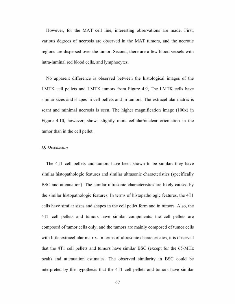
67
However, for the MAT cell line, interesting observations are made. First,
various degrees of necrosis are observed in the MAT tumors, and the necrotic
regions are dispersed over the tumor. Second, there are a few blood vessels with
intra-luminal red blood cells, and lymphocytes.
No apparent difference is observed between the histological images of the
LMTK cell pellets and LMTK tumors from Figure 4.9, The LMTK cells have
similar sizes and shapes in cell pellets and in tumors. The extracellular matrix is
scant and minimal necrosis is seen. The higher magnification image (100x) in
Figure 4.10, however, shows slightly more cellular/nuclear orientation in the
tumor than in the cell pellet.
D) Discussion
The 4T1 cell pellets and tumors have been shown to be similar: they have
similar histopathologic features and similar ultrasonic characteristics (specifically
BSC and attenuation). The similar ultrasonic characteristics are likely caused by
the similar histopathologic features. In terms of histopathologic features, the 4T1
cells have similar sizes and shapes in the cell pellet form and in tumors. Also, the
4T1 cell pellets and tumors have similar components: the cell pellets are
composed of tumor cells only, and the tumors are mainly composed of tumor cells
with little extracellular matrix. In terms of ultrasonic characteristics, it is observed
that the 4T1 cell pellets and tumors have similar BSC (except for the 65-MHz
peak) and attenuation estimates. The observed similarity in BSC could be
interpreted by the hypothesis that the 4T1 cell pellets and tumors have similar

68
scattering sites (whether being cell nuclei or whole cells or a combination of both)
given their similar components. The observed similarity in attenuation could be
analyzed in two aspects: the scattering and the absorption (note: attenuation is the
combined effect of both scattering and absorption). The scattering from 4T1 cell
pellets and tumors has been shown to be similar in terms of BSC. The absorptions
are speculated to be similar based on the observation that 4T1 cell pellets and
tumors have similar components and on the fact that acoustic absorption occurs
primarily at the macromolecular level. With similar BSCs and absorptions, it
makes sense that the attenuation estimates are found to be similar for 4T1 cell
pellets and tumors. Therefore, the similarity in ultrasonic characteristics is a result
of the similarity in histopathologic features. The 4T1 cell line represents an
example where the tumor has relatively simple scattering structures such that the
scattering from the tumor could be similar to that from the cell pellet.
In contrast to 4T1, the MAT cell pellets and tumors show different BSC and
attenuation estimates, which can be attributed to their different histopathologic
features. The main difference between MAT cell pellets and tumors histologically
is that regions of necrosis were found in MAT tumors but not in MAT cell pellets.
The scatterers are significantly different in necrotic regions than other regions
where tumor cells are intact. There are no scatterers that are as big as tumor cells
or cell nuclei in necrotic regions. The necrotic areas consist of fragmented
cytoplasm and nuclei rather than intact nuclei and cytoplasm with definite shape.
This fragmented cellular material is of variable size. Therefore, necrosis can be an
important factor causing the BSC estimates to be significantly different in the

69
MAT tumors versus cell pellets. In addition to BSC, the absorptions are likely to
be different as well, due to necrosis in MAT tumors. With different BSCs and
absorptions, it makes sense that the attenuation estimates are different for MAT
cell pellets and tumors. Therefore, MAT is an example where the tumor is more
complex than the cell pellet and the anatomic structures such as necrosis are
playing a role in scattering.
The situation for LMTK is different from the above two cases. The LMTK cell
pellets and tumors have similar histopathologic features and similar attenuation
results. The similarity in attenuation suggests that the macromolecular
components are similar in the two types of media. The BSC behaviors are
dramatically different, however. The BSC values are closer to each other for
LMTK cell pellets and tumors at lower frequencies (<25 MHz). This might be
explained by the observation that the histopathogic features are similar under the
40x microscope image. The higher degree of cellular/nuclear orientation seen in
the LMTK tumor on the 100x image might be a reason for the BSC discrapency
between the LMTK cell pellets and the tumors at higher frequencies. Again, the
structure function might be playing a role here. A higher degree of cellular
orientation could mean the cell positions are more random.
The comparison between tumors and cell pellets of the same cell lines has
provided insights into the scattering in tumors: (1) the 4T1 result is encouraging
in the sense that it demonstrates the scattering from tumors of homogeneous
morphology can be as similar as the scattering from the cell pellets of the same
cell lines. The scattering model theories for such tumors can be developed by
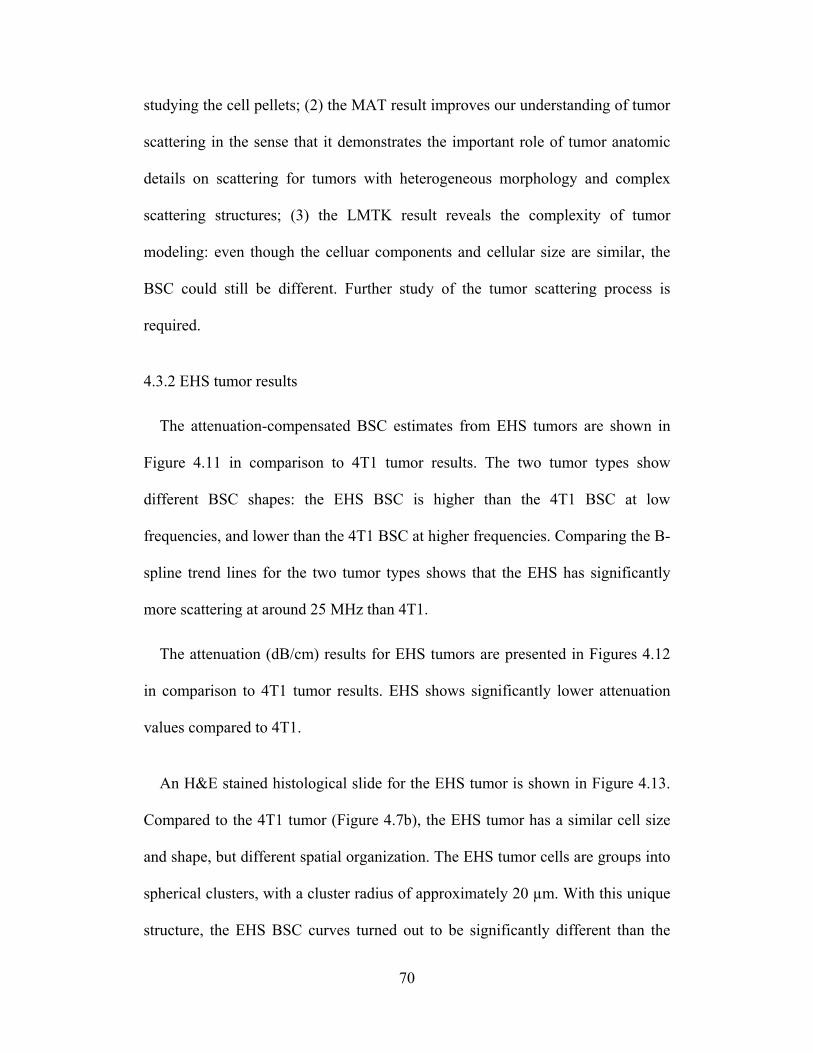
70
studying the cell pellets; (2) the MAT result improves our understanding of tumor
scattering in the sense that it demonstrates the important role of tumor anatomic
details on scattering for tumors with heterogeneous morphology and complex
scattering structures; (3) the LMTK result reveals the complexity of tumor
modeling: even though the celluar components and cellular size are similar, the
BSC could still be different. Further study of the tumor scattering process is
required.
4.3.2 EHS tumor results
The attenuation-compensated BSC estimates from EHS tumors are shown in
Figure 4.11 in comparison to 4T1 tumor results. The two tumor types show
different BSC shapes: the EHS BSC is higher than the 4T1 BSC at low
frequencies, and lower than the 4T1 BSC at higher frequencies. Comparing the B-
spline trend lines for the two tumor types shows that the EHS has significantly
more scattering at around 25 MHz than 4T1.
The attenuation (dB/cm) results for EHS tumors are presented in Figures 4.12
in comparison to 4T1 tumor results. EHS shows significantly lower attenuation
values compared to 4T1.
An H&E stained histological slide for the EHS tumor is shown in Figure 4.13.
Compared to the 4T1 tumor (Figure 4.7b), the EHS tumor has a similar cell size
and shape, but different spatial organization. The EHS tumor cells are groups into
spherical clusters, with a cluster radius of approximately 20 µm. With this unique
structure, the EHS BSC curves turned out to be significantly different than the
71
4T1 curves. The excessive scattering at 25 MHz seems to have come from the
spherical clustering structure: 25 MHz corresponds to a ka value of 2 for a 20-µm
radius.
In addition to the unique spherical clustering structure, the EHS tumor appears
to have more extracellular matrix than any other tumor types discussed in this
chapter so far. Extracellular matrix has different macromolecular components
than tumor cells, which might be the reason why the EHS attenuation is
significantly lower than the 4T1 tumor attenuation.
The EHS results demonstrate how detailed tumor structure could affect
ultrasound backscatter characteristics. Scattering models that appropriately takes
into account these structure details will have great potential in tumor
characterization.
4.3.3 Spontaneous fibroadenoma results
Four rats that had spontaneous fibrous tumors were evaluated, and three of
them were diagnosed from histology to have fibroadenoma. The BSC and
attenuation results from those three rats are presented in this subsection. Unlike
the MAT, 4T1, or LMTK tumors, each of the spontaneous fibroadenoma tumors
had a much larger size (greater than 10 mm in diameter). Therefore, three samples
were trimmed from each tumor at different locations, and a total of nine samples
from three tumors (animals) were scanned and evaluated.

72
The BSC and attenuation results for the three animals are shown in Figure 4.14
and Figure 4.15, respectively. The BSC figure shows that Animal 1 has a
significantly higher BSC in the tumor than Animal 2 does. Both Animal 1 and
Animal 2 have a steeper BSC versus frequency slope than Animal 3 does. The
attenuation figure shows that both Animal 1 and Animal 2 have a much higher
attenuation that Animal 3 does. Also, the within-animal variance in attenuation is
much less than the cross-animal variance. Histology analysis found that the
tumors for Animals 1 and 2 were mostly infarcted and hyalanized, whereas the
tumor for Animal 3 was not (Figure 4.16). The histopathologic feature suggests
that high-frequency ultrasound is sensitive to different disease conditions for the
same disease, as long as the tissue structure changes with disease conditions.
4.3.4 Discussion on the ex vivo condition
The tumor results that have been discussed in this chapter were obtained from
ex vivo scans. Working on ex vivo tumors has both advantages and disadvantages.
The excised tumor samples allow for accurate attenuation estimation using the
insertion-loss technique. Also, the excised tumor samples can be trimmed such
that no skin layer is present in the acoustic path, which eliminates the problem of
compensating for transmission loss. Furthermore, working on ex vivo samples
allows for the study of high-frequency data. It is not feasible to scan the tumors in
vivo using high-frequency (e.g., 80 MHz) single-element transducers. The
disadvantage of working on the ex vivo data is that the ex vivo condition could be
different from the in vivo condition. For instance, there is blood supply in vivo,

73
but not ex vivo, which could cause the scattering to be different. Therefore, the ex
vivo BSC results do not necessarily represent the in vivo BSC results.
To get a sense of how close the ex vivo BSC results are to the in vivo results,
the ex vivo BSC results for the 4T1 and MAT tumors discussed in Section 4.3.1
are compared to the in vivo BSC results from another study [58]. In [58], thirteen
4T1 tumors and eight MAT tumors were scanned in vivo using three imaging
systems and five transducers covering the frequency range 3–22 MHz. This
frequency range has some overlap with the bandwidth of the 20-MHz transducer
used for the ex vivo scans in this dissertation. Therefore, the B-spline fits of the
MAT and 4T1 tumor BSC results from the 20-MHz transducer were compared to
the B-spline fits of the in vivo BSC results from [58]. Figure 4.17 shows the result
of this comparison. The in vivo and ex vivo BSC results were similar for the 4T1
tumors. The in vivo MAT tumor BSC appears to be slightly higher than the ex
vivo MAT tumor BSC.
4.4 Chapter Summary
This chapter summarizes the high-frequency attenuation and BSC results from
various tumor types. The comparison between tumors and cell pellets of the same
cell types provides a start point for accurately model tumor scattering. The fact
that MAT and LMTK each has different BSCs between the tumor and the cell
pellet suggests a closer analysis between the cell pellet and the tumor is required
to proceed with tumor scattering modeling. The EHS and fibroadenoma results
provide more examples of how unique tumor structures can affect the BSC, which
presents opportunities for tumor modeling as well. More detailed analysis of the

74
tumor structures, structure functions, and modeling will be discussed in Chapters
5 and 6.
4.5 Figures
Figure 4.1 BSC versus frequency for five 4T1 cell pellets (blue) and fifteen 4T1 tumor samples (red). The two B-spline curves show the trend shapes for the cell pellets and tumors, respectively.

75
Figure 4.2 BSC versus frequency for five MAT cell pellets (blue) and thirteen LMTK tumor samples (red). The two B-spline curves show the trend shapes for the cell pellets and tumors, respectively.

76
Figure 4.3 BSC versus frequency for three LMTK cell pellets (blue) and thirteen LMTK tumor samples (red). The two B-spline curves show the trend shapes for the cell pellets and tumors, respectively.

77
Figure 4.4 Attenuation (dB/cm) versus frequency for five 4T1 cell pellets (blue) and fifteen 4T1 tumor samples (red).

78
Figure 4.5 Attenuation (dB/cm) versus frequency for five MAT cell pellets (blue) and thirteen MAT tumor samples (red).

79
Figure 4.6 Attenuation (dB/cm) versus frequency for three LTMK cell pellets (blue) and thirteen LMTK tumor samples (red).
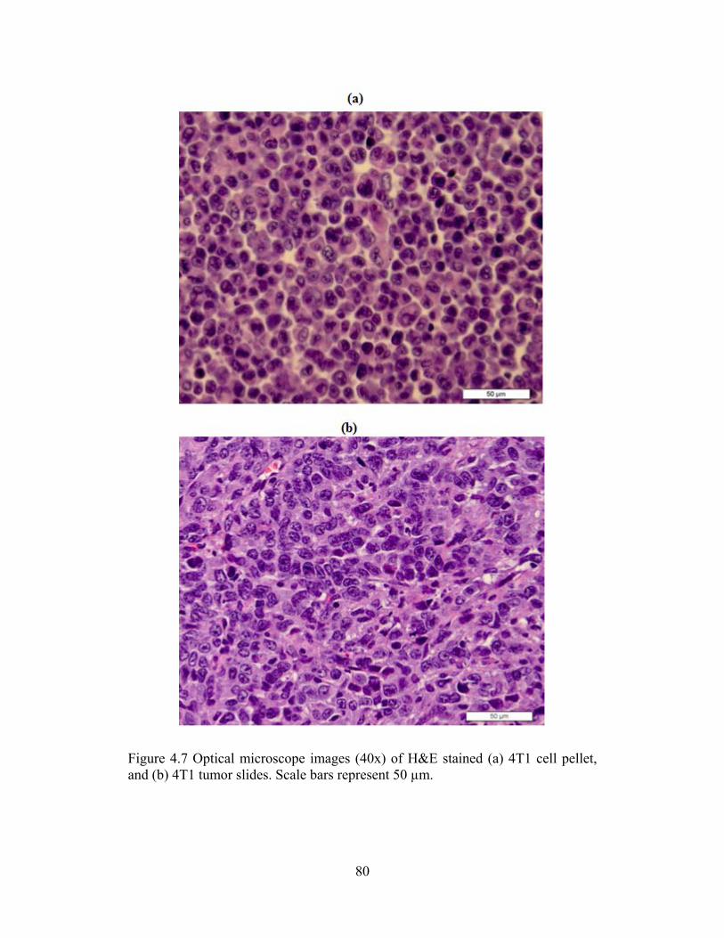
80
Figure 4.7 Optical microscope images (40x) of H&E stained (a) 4T1 cell pellet, and (b) 4T1 tumor slides. Scale bars represent 50 µm.
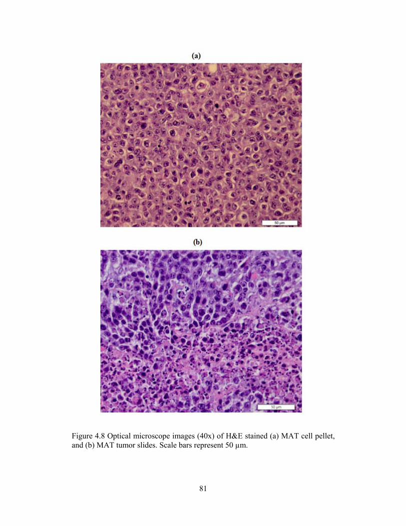
81
Figure 4.8 Optical microscope images (40x) of H&E stained (a) MAT cell pellet, and (b) MAT tumor slides. Scale bars represent 50 µm.
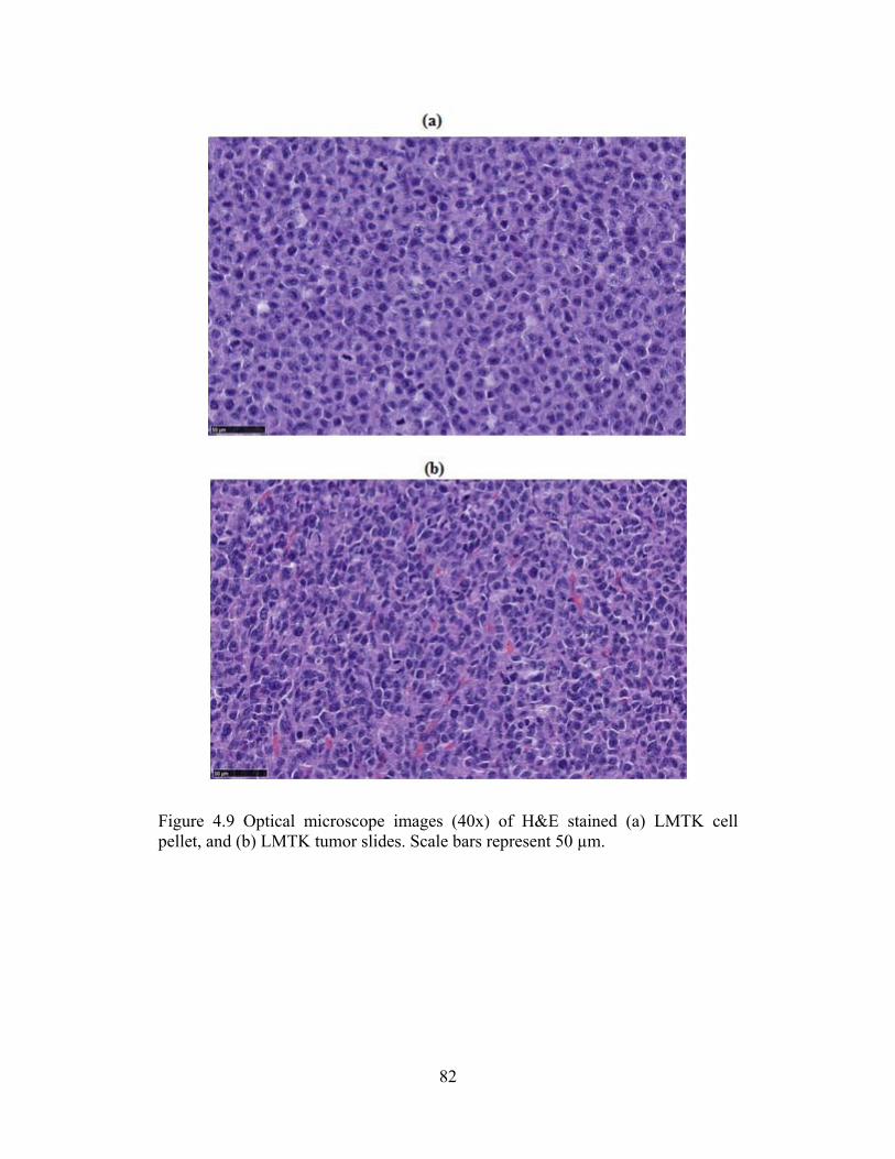
82
Figure 4.9 Optical microscope images (40x) of H&E stained (a) LMTK cell pellet, and (b) LMTK tumor slides. Scale bars represent 50 µm.

83
Figure 4.10 Optical microscope images (100x) of H&E stained (a) LMTK cell pellet, and (b) LMTK tumor slides. Scale bars represent 20 µm.

84
20 40 60 80 1001E-4
1E-3
0.01
0.1
4T1 - experimental EHS - experimental 4T1 - B-spline EHS - B-splineB
SC
[1/(
cm-s
r)]
Freq (MHz)
Figure 4.11 BSC versus frequency for EHS tumors (red) in comparison with 4T1 tumors (blue). The two B-spline curves show the trend shapes for the EHS (gray) and 4T1 (black), respectively.

85
20 40 60 80 100
20
40
60
80
100
120
140
Atte
nuat
ion
(dB
/cm
)
Freq (MHz)
4T1 - 20 MHz 4T1 - 40 MHz 4T1 - 80 MHz EHS - 20 MHz EHS - 40 MHz EHS - 80 MHz
Figure 4.12 Attenuation (dB/cm) versus frequency for EHS tumors (red) in comparison with 4T1 tumors (blue).
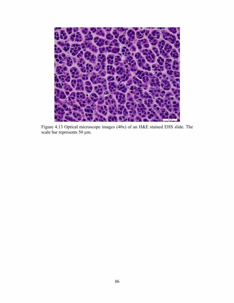
86
Figure 4.13 Optical microscope images (40x) of an H&E stained EHS slide. The scale bar represents 50 µm.

87
Figure 4.14 BSC versus frequency for nine fibroadenoma samples from three animals (rats) evaluated using the 20- and 40-MHz transducers.

88
Figure 4.15 Attenuation (dB/cm) versus frequency for nine fibroadenoma samples from three animals (rats) evaluated using the 20- and 40-MHz transducers.

89
Figure 4.16 Optical microscope images (40x) of H&E stained rat fibroadenoma slides: (a) infarcted and hyalanized, from Animal 1, and (b) not infarcted or hyalanized, from Animal 3. Scale bars represent 50 µm.

90
Figure 4.17 Comparison between the in vivo and ex vivo B-spline BSC curves for 4T1 and MAT tumors. The in vivo results were adapted from Figure 2 of [58], where the blue solid is the B-spline fit to the BSC results obtained from thirteen 4T1 tumors scanned in vivo using three imaging systems and five transducers, and the pink solid is the B-spline fit to the BSC results from eight MAT tumors scanned in vivo using the same imaging systems and transducers. 90% confidence interval is displayed for the in vivo results. The ex vivo B-spline curves (blue dashed for 4T1 and red dashed for MAT) were obtained from BSC results acquired by the 20-MHz transducer (Figures 4.1 and 4.2). No confidence interval is displayed for the ex vivo results for clarity.
.

91
CHAPTER 5
ESTIMATING STRUCTURE FUNCTION FROM HISTOLOGICAL TISSUE SECTIONS
This chapter discusses the estimation of structure function from histological
tissue sections. The 2D structure functions are estimated for high-concentration
cell pellets and tumors. The structure function estimated from the cell pellet
histological tissue sections is related to the experimental and theoretical structure
functions discussed in Chapter 3. The estimated structure function for tumors is
compared to that for cell pellets to give insight into how tumor structures are
affecting acoustic scattering. The structure functions related to unique structures
are discussed. Also mentioned in this chapter is the 2D pair correlation function
extracted from the histological tissue sections to help understanding the structure
function.
5.1 Background and Introduction
In Chapter 3, the structure function has been estimated for high-concentration
cell pellets from the BSC data. The estimated structure function curve has been
attributed to the possibility that the high-concentration condition makes the spatial
arrangement of cell positions less random than it would be for low concentrations.
Two polydisperse structure function models have been developed to describe the
effect of high concentration on cell spatial arrangement and the structure function.
The models theoretically predict a structure function curve that agrees well with

92
the experimental one, particularly in terms of the peak position. However, the
models are not direct evidence to support the hypothesis that the structure
function curves estimated from the BSC curves are a result of the cell spatial
position correlation.
To provide direct evidence, we plan to examine the histological sections of the
samples. Ideally, if the 3D cell positions are known, the exact structure function
can be calculated using Equations (2.13) – (2.14). Unfortunately, determining the
3D cell positions is very difficult and may not be feasible. A less ideal alternative
would be to study the cell positions in 2D and determine the 2D structure function
SA(2k), where the subscript A represents 2D (area). Precisely relating the 2D
structure function estimated from a thin section of finite thickness to the actual 3D
structure function is a difficult stereological problem, and to date there is no
generally applicable solution. However, studying the 2D structure function may
provide a qualitative comparison between the cell position correlation and the
backscattered data.
In addition to the structure function, the 2D pair correlation function A ( )g r can
be determined from the tissue sections as well. The pair correlation function
provides a more intuitive way of understanding the spatial distribution of cells. In
3D, the pair correlation V ( )g r for a particular distribution of particles is defined as
the probability of finding a particle at distance of r away from a given reference
particle, relative to that for a distribution of completely uncorrelated particles.
Therefore, V ( ) 1g r for a distribution of uncorrelated particles. If the particle
positions are correlated, the local number density at a distance r from the

93
reference particle is determined by V ( )ng r , where n is the average number
density of the entire system. The concept is the same for 2D. For an isotropic
distribution of spheres of similar size, the pair correlation function A ( )g r
estimated from a 2D section is a rough approximation for the 3D pair correlation
function V ( )g r [59].
Estimating the structure function and pair correlation function from histological
slides will eventually improve the understanding of tumor scattering. Chapter 4
points out that the BSC curves can be different for cell pellets and tumors of the
same cell line (e.g., LMTK), although both the cell pellets and tumors are
composed of primarily the same type of cells. It is hypothesized that the
difference in BSC might have come from the difference in the spatial distribution
of tumor cells. The 2D histological section study will provide an opportunity to
test the hypothesis by exploring exactly how the distribution is different.
Furthermore, the cell spatial distributions for different tumor structures can be
compared, which will provide guidelines for tumor structure modeling.
5.2 Methods
An H&E stained tissue section was viewed under a light microscope (Olympus
BX–51, Optical Analysis Corporation, Nashua, NH, USA). For each tissue slide,
a 40 X TIF format picture was taken using the digital camera that was in sync
with the microscope (see Figure 4.13 for a typical picture). Each image contained
a 50 µm scale bar on the lower right of the image. The dimension of the image
was 2560 × 1920 pixels, with a resolution of 5.72 pixels per micron. Only an area

94
of 1920 × 1920 pixels was analyzed for pair correlation and structure function
estimation. This area covers the majority of the original image except a 640 ×
1920 rectangle on the right side that contains the scale bar. The analyzed image
area corresponds to a physical dimension of 336 × 336 µm2. For each scanned
biological sample type, two to three pictures from separate tissue sections were
taken and analyzed.
A custom MATLAB routine was developed to allow manual determination of
the nuclear center for each cell on the image (the nucleus center was assumed to
overlap the cell center). The manual determination process was completed by
clicking on the nucleus center on the image opened in MATLAB (Figure 5.1).
The nuclear center coordinates were automatically recorded for further
processing. As an example, 700 nuclear centers were found from the image shown
in Figure 5.1, and plotted separately in Figure 5.2.
5.2.1 Structure function estimation
A matrix of the dimension 1920 × 1920 was created. The matrix dimension was
the same as the pixel dimension of the image (Figure 5.1). The matrix elements
that were corresponding to nuclear centers were assigned a value of one, with all
remaining matrix elements being assigned a value of zero. The nuclear centers
were essentially gridded. The gridding will not cause a problem because the
gridding resolution (5.7 µm-1) is sufficiently high compared to the cell/nuclear
size. A fast Fourier transform was performed on the matrix. The squared modulus
of the 2D Fourier transform (Figure 5.3), normalized to unity for large wave
numbers, is the 2D structure function for all directions. A radial symmetry of the

95
structure function is observed, suggesting the isotropy of the system. Therefore, a
radial averaging was performed, which resulted in a structure function A ( )S k that
is only dependent on the modulus of the wave number. For backscattering, we are
interested in A (2 )S k . Converting k to frequency in MHz using a speed of sound
1540 m/s will generate the frequency-dependent 2D structure function (e.g.,
Figure 5.4).
5.2.2 Pair correlation function estimation
The pair correlation function was estimated using the algorithm described in
[60]. The algorithm is briefly summarized as follows. To calculate A ( )g r , a value
of distance resolution dr was picked first. The distance resolution cannot be too
small because of limited number of points on the 2D image (Figure 5.2). It cannot
be too large either, to avoid blurring any important structures in the pair
correlation curve. A distance resolution of 0.87 µm (equivalent to five pixels of
the original image) was chosen. For each distance r at which the pair correlation
function was to be calculated, each nuclear center was chosen as a reference point
in turn. The number of nuclear centers that were at a distance between r and r + dr
away from the reference point was counted, and averaged for all the reference
points. This number was then normalized by 2 rdr (the area of the ring), and
divided by the average number of nuclear centers per unit area. The edge effect
was also properly accounted for. Specifically, when calculating the pair
correlation function based on reference nuclear centers near the edge of the
image, the circle of some radius r may extend outside the image. The edge effect
was correctly accounted for by determining how much angular extent of the circle

96
lies within the image. An example of estimated pair correlation function is shown
in Figure 5.5.
5.3 Results and Discussions
5.3.1 Simulations
For comparison purposes, the estimated pair correlation functions and structure
functions from three simulated point distributions are presented herein, before
presenting the results from the tissue histological images. The three simulated 2D
point distributions are: (a) the points are randomly distributed in the image
(Figure 5.6a); (b) the points are clustered, with weaker clustering (Figure 5.6b);
and (c) the points are clustered, with stronger clustering (Figure 5.6c). The same
number density is used for the three simulations (900 points on a 336 × 336 µm2
area).
The pair correlation function extracted from Figure 5.6a is approximately unity
over the entire range of analyzed distance (Figure 5.7), as expected. The two
clustering point distributions yield pair correlation functions that have high values
at closer distances, and the pair correlation function gradually reduces to unity as
the distance increases (Figure 5.7). The primary effect of clustering is the
increased pair correlation function at closer distances. The stronger the clustering
is, the higher the pair correlation function is at closer distances.
Similarly, the structure function extracted from Figure 5.6a is approximately
unity over the entire frequency range being analyzed. Clustering increases the

97
lower-frequency component of the structure function. The strong clustering is, the
higher the low-frequency structure function is (Figure 5.8).
The simulation results are presented for two reasons. The simulation results
allow for comparison between simulations and the actual results from tumors.
More importantly, the results demonstrate the feasibility of extracting the pair
correlation function and structure function from a 2D region of similar
dimensions and numbers of points.
5.3.2 Cell pellets
The estimated 2D structure function curves are presented in Figure 5.9 for
high-concentration (74% volume fraction; same as Concentration II in Chapter 3)
cell pellets of four cell lines: CHO, MAT, 4T1, and LMTK. The general trend of
the 2D structure function curves appears to be similar to the structure function
calculated from the ultrasonic scattering data (Figure 3.6), and to the polydisperse
structure function curves in Chapter 3.
A one-to-one comparison between the 2D structure function and the structure
function from ultrasonic scattering is shown in Figure 5.10, Figure 5.11, and
Figure 5.12 for CHO, MAT, and 4T1, respectively. The peak position agree very
well (within 5 MHz) between the two structure function curves for each of the
three cell lines. The shape agreement is also observed for CHO and MAT. The
magnitude agreement is not as good; only MAT shows good agreement in
structure function curves (Figure 5.11). For CHO, the acoustic structure function
is in general lower than the 2D structure function across the frequency range
(Figure 5.10). The peak magnitude barely exceeds unity for the acoustic structure

98
function for CHO. The acoustic structure function curve could have been under
estimated due to number density uncertainty, etc.
In general, the 2D structure function curves at least show convincing qualitative
agreement with the curves and theories presented in Chapter 3. Also, the peak
position of the 2D structure function curve shows good correlation with cell size:
4T1 has the largest cell size (cell radius: 8.9 µm) out of the four cell lines,
whereas the other three cell lines have similar but smaller cell sizes (cell radius:
6.8, 7.3, and 7.3 µm for CHO, MAT, and LMTK, respectively). Therefore, the
structure function peak for 4T1 is at the lowest frequency compared to other cell
lines, and the structure function peak of the other cell lines are located at similar
frequencies.
The estimated pair correlation curves (Figure 5.13) for the four cell lines give
insight into what aspects of cell arrangement have cause the structure function
behavior. All four cell lines have a zero pair correlation for
approximately 5r m . This is because the cells are considered non-overlapping
spheres. The width of the zero-correlation region is determined by the cell
diameter. The 4T1 curve has the widest zero-correlation region because of the
large cell radius. Note that the 2D pair correlation function is only a very rough
approximation of the 3D case, because cells at different depths could appear to be
slightly overlapping in 2D, reducing the width of the zero-correlation regions.
Although very significant, the non-overlapping condition alone is not the reason
for the observed structure function behavior. What has caused the observed
structure function behavior is a combination of the non-overlapping condition and

99
the high concentration. Because of the high concentration, the pair correlation
curve immediately sees a sharp peak above unity after the zero-correlation region.
If the cell concentration had been much lower, then the sharp peak could not have
been observed, and the resulting structure function curve would have been closer
to unity.
5.3.3 Tumors versus cell pellets
The structure function and pair correlation function were estimated for 4T1,
MAT, LMTK, and EHS tumors. Necrotic regions were not analyzed for MAT
tumors, because it is hard to find the nuclear center in the necrotic region.
Therefore, the MAT results may not fully reflect the entire MAT tumor structure.
The tumor structure functions are compared to the cell pellet structure functions
for 4T1, MAT, and LMTK (Figure 5.14). The tumors appear to have less structure
function effect than the cell pellets do. The tumor has a lower structure function
than the cell pellet of the same cell type at frequencies lower than 50 MHz,
meaning that the tumor cell arrangement has a less destructive effect in the
destructive frequency range. In the constructive frequency range (around the
scattering peak), the tumor shows a less constructive effect as well. The observed
2D structure functions in Figure 5.14 are well correlated to the BSC curves in
Figures 4.1 – 4.3 also. Overall the tumor structure function curves are smoother
than the cell pellet curves. This could suggest that the cell arrangement is more
random in tumors than in cell pellets.
The pair correlation function comparison between cell pellets and tumors
(Figure 5.15) shows three important features: (a) the zero-correlation region is

100
wider for the cell pellets than for the tumor; (b) the correlation peak occurs at a
closer distance for the tumor than for the cell pellet; (c) the peak values are higher
for the cell pellet than for the tumor. The three features reveal the structural
difference between cell pellets and tumors. Feature (a) might be explained by the
fact that some cells may be pushed in tumors so that the centers between certain
cell pairs are shortened. The same reason could be attributed to feature (b).
Feature (c) suggests that the cell arrangement in tumors is more random than in
cell pellets, consistent with structure function observation.
5.3.4 EHS and clustering
The EHS tumor is different from 4T1, MAT, and LMTK in the cell
arrangement: the cells are grouped in EHS, with typically less than 20 cells per
group, whereas other tumors do not show such a clustering phenomenon. To show
how cell clustering affects the structure function in tumors, the 2D structure
functions are compared for all the four tumor types (Figure 5.16). The tumor
structure functions seem to be similar, except that the EHS show higher structure
function values around 25 MHz compared to other tumor types. This phenomenon
can explain the experimental BSC behavior of EHS compared to other tumor
types (e.g., Figure 4.11): EHS shows more scattering at around 25 MHz than
other tumor types. Therefore, the results suggest that the additional scattering at
25 MHz for EHS is related to the EHS tumor cell arrangement.
The pair correlation function comparison between EHS and other tumor types
(Figure 5.17) provides more detailed information about cell spatial arrangement.
EHS has a slightly higher peak around 10 µm than other tumor types. More

101
interestingly, there is a dip around 15 µm in the EHS curve but not in other tumor
curves (Figure 5.17). This dip might be a result of the clustering structure. There
is empty space between different clusters, resulting in decreased probability of
finding a nuclear center in that space. If this hypothesis is true, then the dip
position would be related to the cluster size.
Comparing the EHS pair correlation function with the simulation results for
clustered points (Figure 5.7), it is hard to find any similarity between the two. In
fact, the EHS pair correlation function appears to be more similar to that of non-
clustering tumors (although noticeable difference exists). Note that non-
overlapping condition was not applied to the simulations. Therefore, the
comparison between EHS and simulation results suggests that the effect of
clustering on structure function is significantly reduced due to the non-
overlapping condition. Also, the close distance between the EHS tumor clusters
may have further reduced the effect of clustering on structure function.
5.3.5 Significance and limitations
The 2D structure function and pair correlation function estimated from
histological sections provide direct evidence to show that the cell spatial
arrangement affects acoustic scattering in real tumors. The result also
qualitatively confirms the polydisperse structure function model developed in
Chapter 3. It provides guidelines as to how to model the structure function
properly. Overall the results significantly improved the understanding of how
tumors scatter ultrasound.

102
However, there are several limitations in the 2D histological section study.
First, the 2D structure function and pair correlation function are not exactly the
same as those in 3D. Therefore, we would not be able to directly divide the BSC
by the 2D structure function to estimate the incoherent BSC. Second, the number
of histological sections analyzed for each sample type is not large enough. Only
three images on average have been analyzed for each sample type. Third, manual
determination of the nuclear center is time-intensive, and subject to human error.
Automatic procedures are currently not available.
5.4 Chapter Summary
This chapter has introduced histology analysis methods that can be used to
relate histological features to scattering and the structure function. The method of
extracting the 2D structure function and pair correlation function from
histological sections is shown to be feasible. The 2D structure function and pair
correlation function have been successfully estimated from 2D histological
sections for various sample types. The comparisons among different sample types
improve our understanding of how tumor microstructure (particularly cell
arrangement) affects scattering. Specifically, the tumor cells are shown to be more
randomly distributed than in cell pellets. Tumor cell clustering is shown to
moderately affect the structure function, and should be taken into consideration
when scattering models are being developed.

103
5.5 Figures
Figure 5.1 An optical microscope image (40x magnification; 1920 × 1920 pixels) superimposed with nuclear centers in yellow dots that were manually determined. Displayed are 700 nuclear center points.

104
Figure 5.2 Nuclear centers extracted from Figure 5.1 plotted on the XY plane. The coordinates were gridded (sampled), with a spatial sampling rate of 5.7 µm-1.

105
Figure 5.3 Two-dimensional plot of the squared modulus of the fast Fourier transform of the points plotted on Figure 5.2.

106
Figure 5.4 An estimated structure function versus frequency curve, obtained by radial averaging of the modulus of the 2D Fourier transform shown in Figure 5.3.

107
Figure 5.5 An estimated pair correlation function versus distance curve, obtained from points presented in Figure 5.2.

108
Figure 5.6 Simulated 2D distributions of random points for, (a) a completely random distribution, (b) a clustering distribution with weaker clustering, and (c) a clustering distribution with stronger clustering.

109
Figure 5.7 Estimated pair correlation functions from the point distributions shown in Figure 5.6.

110
Figure 5.8 Estimated structure functions from the point distributions shown in Figure 5.6.

111
Figure 5.9 Comparison among the average estimated structure functions from the histological sections for high-concentration CHO, 4T1, MAT, and LMTK cell pellets. Each curve is an average of three independent measures on different histological images.

112
Figure 5.10 Comparison between the 2D structure function estimated from histological slides and the structure function obtained from ultrasonic backscattering coefficients (see Figure 3.6a) for high-concentration CHO cell pellets. The blue curve is an average of three independent measures on different histological images.
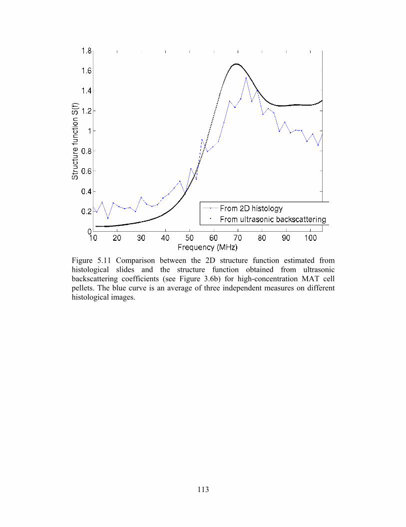
113
Figure 5.11 Comparison between the 2D structure function estimated from histological slides and the structure function obtained from ultrasonic backscattering coefficients (see Figure 3.6b) for high-concentration MAT cell pellets. The blue curve is an average of three independent measures on different histological images.

114
Figure 5.12 Comparison between the 2D structure function estimated from histological slides and the structure function obtained from ultrasonic backscattering coefficients (see Figure 3.6c) for high-concentration 4T1 cell pellets. The blue curve is an average of three independent measures on different histological images.

115
Figure 5.13 Comparison among the average estimated pair correlation functions from the histological sections for high-concentration CHO, 4T1, MAT, and LMTK cell pellets. Each curve is an average of three independent measures on different histological images.

116
0 20 40 60 80 100 1200
1
2(a)
Str
uctu
re f
unct
ion
S A(f
)
4T1 Cell Pellet4T1 Tumor
0 20 40 60 80 100 1200
1
2(b)
MAT Cell PelletMAT Tumor
0 20 40 60 80 100 1200
1
2(c)
Frequency (MHz)
LMTK Cell PelletLMTK Tumor
Figure 5.14 Comparison between the average 2D structure function curves for (a) 4T1 cell pellets and tumors, (b) MAT cell pellets and tumors, and (c) LMTK cell pellets and tumors.

117
0 5 10 15 20 25 30 350
1
2(a)
Pai
r co
rrel
atio
n fu
nctio
n g A
(r)
4T1 Cell Pellet4T1 Tumor
0 5 10 15 20 25 30 350
1
2(b)
MAT Cell PelletMAT Tumor
0 5 10 15 20 25 30 350
1
2(c)
r (m)
LMTK Cell PelletLMTK Tumor
Figure 5.15 Comparison between the average pair correlation curves for (a) 4T1 cell pellets and tumors, (b) MAT cell pellets and tumors, and (c) LMTK cell pellets and tumors.

118
0 20 40 60 80 100 1200
0.2
0.4
0.6
0.8
1
1.2
1.4
Frequency (MHz)
Str
uctu
re f
unct
ion
S A(f
)
4T1 Tumor
MAT TumorLMTK Tumor
EHS Tumor
Figure 5.16 Comparison among the average 2D structure function curves for 4T1, MAT, LMTK, and EHS tumors.

119
0 10 20 30 400
0.5
1
1.5
r (m)
Pai
r co
rrel
atio
n fu
nctio
n g A
(r)
4T1 Tumor
MAT TumorLMTK Tumor
EHS Tumor
Figure 5.17 Comparison among the average 2D pair correlation function curves for 4T1, MAT, LMTK, and EHS tumors.
120
CHAPTER 6
TUMOR SCATTERING MODELING
This chapter discusses modeling the scattering of different tumor structures.
Two cases are considered herein, the tumor cells are homogenously distributed
(e.g., 4T1, LMTK), and the tumor cells are clustered (e.g., EHS). The effect of
the structure function on scatterer parameter estimation is discussed. A new
scattering model that is capable of detecting tumor cell clustering is developed.
6.1 Background and Introduction
Commonly used scattering models for tumors are based on the assumption that
the scatterer positions are uncorrelated. The fluid-filled sphere model and the
Gaussian form factor model are two such examples. For these two models, the
BSC is determined by two parameters, the effective scatterer size and the
effective acoustic concentration (EAC). The EAC is the product of the number of
scatterers per unit volume and the square of the fractional change in the
impedance between the scatterer and the surrounding medium. The effective
scatterer size affects the slope and the magnitude of the BSC versus frequency
curve. The EAC only affects the magnitude of the BSC curve.
Previous chapters have shown that the spatial correlation among scatterer
positions in tumors plays a significant role in scattering, and modifies the BSC
curve substantially. Therefore, models such as the fluid-filled sphere model and

121
the Gaussian form factor model may not give accurate parameter estimates. It is
important to evaluate how the structure function affects model parameter
estimates, by comparing the parameters estimated using models that do not take
into account the structure function versus parameters estimated using models that
take into account the structure function. Also, a comparison between different
structure function models would be interesting.
For the above reasons, three models are compared in this chapter to evaluate
the effect of structure function on parameter estimates: the fluid-filled sphere
model (denoted FF), the fluid-filled sphere model incorporating the structure
function estimated from 2D histological slides (denoted SF0), and the fluid-filled
sphere model incorporating a polydisperse structure function (denoted SF1; the
polydisperse structure function is Polydisperse Model I described in Chapter 3).
SF0 is included in comparison because the 2D structure function estimated from
histology is the only available structure function estimated directly from tumors,
although 2D and 3D can be different. SF1 is included in comparison because it is
a theoretical model that works reasonably well for high-concentration cell pellets
at high frequencies where there is a peak in the BSC curve. The theoretical
structure function used in SF1 is not the same curve as the estimated 2D structure
function used in SF0. Therefore, SF0 and SF1 represent two different structure
function models.
The structure function for tumors with cell clustering is different than that for
tumors that have a homogenous cell distribution (Figure 5.16). SF1 is developed
for a homogenous cell distribution, but not for a clustering structure. A model that

122
is capable of detecting the clustering structure is desirable. For the EHS tumors,
the clustering of cells not only changes the structure function, but may also alter
the scattering sites as well – the cell clump may become a scattering site as well
because of possible impedance contrast between the clump and the extracellular
matrix. Therefore, a model that assumes two primary scatter sizes is developed for
the EHS tumor and is applied for detecting clustering.
6.2 Effect of Structure Function on Model Parameter Estimation
6.2.1 Methods
Three models (FF, SF0, SF1) are applied to the experimental BSC data from
MAT, 4T1, LMTK, and EHS tumor data. The scatterers are assumed to follow a
gamma distribution as described in Equation (3.2). To reduce the number of
unknowns for the inverse problem, the Schulz width factor z is assumed to be 50
for all three models, based on measurements made in Chapter 3.
The first model, FF, is calculated using
2 4 20
1 1(2 ) 1 ' ( '' '')
2 4FFBSC k n k k k , (6.1)
where n is the scatterer number density, 20 is the mean-square variation in
acoustic impedance per scatterer as in Equation (2.5), the product 20n is the
EAC, and the quantities , ' , '' , and '' are defined in Equation (A.5).
Equation (6.1) is an analytical expression of the BSC for fluid-filled spheres with
gamma-distributed radii. Equation (6.1) is a slightly modified form of Equation
(19) in [53].

123
The second model, SF0, is calculated by
0 0(2 ) (2 ) ( )SF FFBSC k BSC k S k , (6.2)
where (2 )FFBSC k is calculated using Equation (6.1), and the structure function
0 ( )S k is assumed to be known, calculated for each tumor type by performing a
seventh-order polynomial fit to the corresponding structure function curve
presented in Figure 5.16.
The third model, SF1, is calculated by
1 1(2 ) (2 ) ( )SF FFBSC k BSC k S k , (6.3)
where the structure function 1( )S k is calculated using Equation (A.1).
The unknowns for model FF are the average radius a and the effective acoustic
concentration EAC (dB/mL). The unknowns for model SF0 are the same as for
model FF. The unknowns for model SF1 are the average radius a, the EAC, and
the volume fraction. A least squares minimization is performed using an
exhaustive search approach, to find parameter values that minimize the mean
square error between the log-scaled experimental and theoretical BSCs.
Considering that the parameter estimation is often dependent on frequency,
three frequency ranges are analyzed: 11 – 31 MHz (data from the 20-MHz
transducer), 11 – 52 MHz (data from the 20- and 40-MHz transducers), and 11 –
105 MHz (data from the 20-, 40- and 80-MHz transducers). Frequency ranges that
contain only the data from 40- or 80-MHz transducers are not used, because the
high-frequency BSC curve for tumors tends to be horizontal.
124
6.2.2 Results
The estimated scatterer radii and effective acoustic concentrations for MAT,
4T1, LMTK, and EHS tumors using the three models are shown in Figure 6.1 (11-
31 MHz), Figure 6.2 (11-52 MHz), and Figure 6.3 (11-105 MHz). The estimated
scatterer volume fraction using model SF1 is shown in Figure 6.4.
Comparing FF and SF0, FF underestimates the scatterer radius or the effective
acoustic concentration in most cases compared to SF0. Comparing SF0 and SF1,
SF0 always underestimates the scatterer radius and overestimates the effective
acoustic concentration, regardless of which frequency range is being used.
Comparing the frequency ranges, all the models tend to have lower radius
estimates and higher EAC estimates. However, the volume fraction estimated
from model SF1 does not show a clear dependence on which frequency range is
used for MAT, 4T1, and LMTK tumors (Figure 6.4). The volume fraction
estimates for those three tumor types are in a reasonable range. The EHS shows a
higher volume fraction estimate than the other tumor types. This observation
allows for distinction between EHS and other tumor types. However, a higher
volume fraction estimate for EHS tumors is not consistent with the fact that EHS
tumors have a greater amount of the extracellular matrix than the other three
tumor types. This inconsistency may be caused by cell clustering in EHS.
6.2.3 Discussions
The comparison among three models shows the model parameter estimates are
sensitive to the structure function. Different estimated values are obtained when
different structure functions are used. The structure function can alter both the
125
magnitude and the frequency dependence of the BSC curve. Therefore, both the
scatterer size and the effective acoustic concentration estimations may be
affected.
For the lower frequency range (11 – 31 MHz, Figure 6.1) typically used in most
QUS studies, the structure function has values that are much lower than unity,
which effectively reduces the BSC magnitude. The widely used FF model that
does not take into account this effect underestimates the effective acoustic
concentration (Figure 6.1b). The SF1 model that works reasonably well for the
high-concentration cell pellets overestimates the effective acoustic concentration
compared to SF0 as a reference, because the structure function in SF1 has values
that are much lower than the measured 2D structure function used in SF0.
Therefore, the polydisperse structure function models developed in Chapter 3
appear to overestimate the regularity of the spatial arrangement of tumor cells.
The polydisperse structure functions work better for cell pellets because the cell
pellets have a more regular cell arrangement than tumors, as is evidence in Figure
5.14 where the cell pellet structure functions are lower than the tumor structure
functions at lower frequencies.
The phenomenon that the estimated scatterer size and effective acoustic
concentration depends on the analysis frequency has been observed frequently in
QUS studies. This dependency is undesirable, because it obscures the biological
meaning of the parameters. Parameters estimates that are independent of analysis
frequency may be more robust for tissue characterization purposes. Model SF1
has an advantage in this aspect because it is capable of generating scatterer
126
volume fraction estimate that is independent of analysis frequency, despite the
fact that the model underestimates the randomness in tumor cell arrangement.
Note that model SF1 is developed for a homogenous distribution of cells, hence
the scatterer volume fraction estimate for EHS tumors is not accurate and can
only be used for classification purpose.
6.3 A Model for the EHS Tumor
This subsection introduces a model that describes the clustering feature of the
EHS tumor cells. The model assumes that the cell clumps are scattering sites in
addition to the individual spheres. The BSC is expressed as:
1/30( ) ( , , ) ( , , )FF FFBSC f BSC a EAC f BSC aN CI EAC f , (6.1)
where FFBSC is the fluid-filled sphere BSC, N is the number of spheres per
cluster, EAC is the acoustic concentration of the spheres, and 0CI is the
clustering index which means the ratio of cluster EAC to sphere EAC in the
model. The size distribution of the spheres may be taken into account in the
model also. For the subsequent analysis, the spherical radius is assumed to follow
a Schulz distribution. A Schulz width factor z = 50 is used to take into account the
polydispersity of the spherical radius.
The reasons why the clustering index 0CI may be used to characterize the
“clustering strength” are the follows: (1) For a given N, if most of the spheres are
not clustered and only a small portion of the spheres are clustered, then the
number density, consequently the EAC, of the clusters would be lower compared
to the case when more spheres are clustered. (2) If the impedance contrast

127
between the clusters and the extracellular matrix is higher, the scattering from the
cluster would be higher as a result.
The proposed model is applied to MAT, 4T1, LMTK, and EHS tumors to
estimate the clustering index 0CI (in dB) of each tumor type (Figure 6.5). The
EHS shows the highest clustering index for all the frequency ranges, suggesting
that the model is able to detect the clustering structure. Also, the MAT shows a
higher clustering index than the 4T1 and LMTK, which might be attributed to the
necrosis in the MAT tumors. The necrosis in the MAT tumors effectively creates
a clustering phenomenon because of missed cells due to necrosis.
6.4 Chapter Summary
The effects of structure function on scatterer parameter estimation have been
discussed. The scatterer radius and effective acoustic concentration of the widely
used fluid-filled sphere model have shown to be sensitive to the choice of
structure function. The polydisperse structure functions developed in Chapter 3
underestimated the randomness of the cell arrangement in tumors. More accurate
structure functions for tumors are required to model tumor scattering more
accurately. As an example of modeling unique tumor structures, the new model
developed for EHS has been shown to be able to detect clustering and model the
clustered tumor cell structure.

128
6.5 Figures
Figure 6.1 (a) Estimated scatterer radii, and (b) estimated effective acoustic concentrations for MAT, 4T1, LMTK, and EHS tumors using three models (FF, SF0, and SF1) in the frequency range of 11 – 31 MHz. The estimated parameter value for a tumor type represents the average from all the samples of that tumor type, and error bars represent the standard deviation.

129
Figure 6.2 (a) Estimated scatterer radii, and (b) estimated effective acoustic concentrations for MAT, 4T1, LMTK, and EHS tumors using three models (FF, SF0, and SF1) in the frequency range of 11 – 52 MHz. The estimated parameter value for a tumor type represents the average from all the samples of that tumor type, and error bars represent the standard deviation.
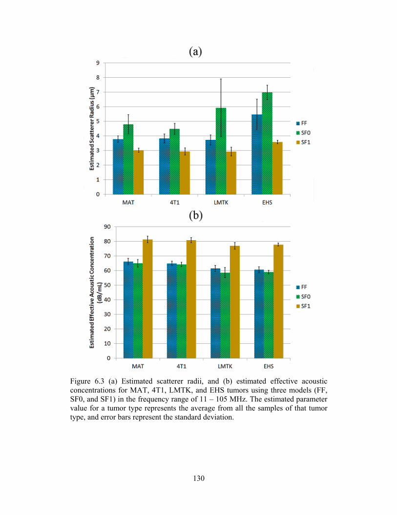
130
Figure 6.3 (a) Estimated scatterer radii, and (b) estimated effective acoustic concentrations for MAT, 4T1, LMTK, and EHS tumors using three models (FF, SF0, and SF1) in the frequency range of 11 – 105 MHz. The estimated parameter value for a tumor type represents the average from all the samples of that tumor type, and error bars represent the standard deviation.

131
Figure 6.4 Estimated volume fractions for MAT, 4T1, LMTK, and EHS tumors using model SF1 in three different frequency ranges. The estimated parameter value for a tumor type represents the average from all the samples of that tumor type, and error bars represent the standard deviation.

132
Figure 6.5 Estimated clustering indexes for MAT, 4T1, LMTK, and EHS tumors in three different frequency ranges. The estimated parameter value for a tumor type represents the average from all the samples of that tumor type, and error bars represent the standard deviation.

133
CHAPTER 7
CONCLUSIONS AND FUTURE WORK
This dissertation investigates the scattering from tumors by studying the
scattering from biological media of different degrees of complexity. Our
understanding of the acoustic scattering processes in tumors has been improved
through this investigation. The comparison between lower and higher
concentrations of cell pellets demonstrates that the concentration affects the
spatial arrangement of cells, and thus the structure function and BSC. The
structure function of high-concentration cell pellets is modeled reasonably well by
the proposed polydisperse structure function models. The comparison between
cell pellets and tumors of the same cell types, and between different tumor types,
reveals that unique tumor structures could have special scattering patterns. The
estimated 2D structure function and pair correlation function from histological
slides confirm the significance of structure function in dense media, support the
proposed structure function models for high-concentration cell pellets, and reveal
the cell arrangement difference between cell pellets and tumors. The unique
clustering tumor structure can be detected using models that take into account the
clustering structure. The modeling of the scattering from tumors with
homogenously distributed tumor cells requires further study. This chapter
concludes the dissertation and suggests possible directions for future studies.

134
7.1 Structure Function Estimation and Modeling for Cell Pellets
The structure function has been isolated from the BSC by comparing two
concentrations of cell pellets. The experiment could be improved by including
more concentrations and extending to lower concentrations. For model validation
purposes, physical phantoms of similar scatterer sizes and concentrations to the
cell pellets could be produced and scanned.
Another future direction could be to study the effect of the finite transducer
beamwidth on the estimation of the structure function. The theories and models
discussed in this dissertation are based on the assumption that the particles are
scanned by a plane wave extending infinitely in space. The sound field produced
by a weakly-focused single-element transducer has a finite boundary. The
scattering volume is thus limited. The structure function of a limited scattering
volume can be different from that of a much larger volume. Theoretical and
experimental studies should address issues such as determining the minimal
required scattering volume for obtaining a satisfactory estimate of the structure
function.
7.2 The Comparison between Cell Pellets and Tumors
The comparison between cell pellets and tumors of the same cell types is the
key to understanding tumor scattering. The observed difference in BSC between
cell pellets and tumors of the same cell types has been attributed to the unique
tumor structures such as regions of necrosis and the presence of blood vessel in
tumors, and the structure function differences between cell pellets and tumors.

135
However, the above factors still do not fully explain why the homogenous
LMTK tumor has an entirely different BSC behavior than the LMTK cell pellet
does. Investigating additional factors that may cause the difference will
significantly improve tumor scattering modeling. Further studies could be focused
on histology analysis. Automatic or semi-automatic image processing techniques
that are capable of detecting objects on a histological image can be developed and
applied to analyze the histology systematically. The idea of object detection
should not be limited to nucleus or cytoplasm. Rather, any object that is of the
scale of interest could be detected and analyzed. Further, different staining
techniques could be explored. Structure differences that cannot be distinguished
by the currently used H&E staining might be seen if another staining method is
applied. Additionally, the two-dimensional impedance map (2DZM) techniques
that are currently being developed by other researchers will have the potential to
be used for identifying the additional factors that caused the difference in
scattering between LMTK cell pellets and tumors.
7.3 Structure Function Estimation from Histological Sections
Directly measuring the structure function from histology is a useful approach to
understanding the structure function. The current study on estimating the structure
function from 2D histological sections could be improved by a number of future
steps. First, more images should be analyzed to yield a more accurate estimation
of the 2D structure function. Different magnifications, different image sizes can
be explored as well. Second, an automatic or semi-manual cell (or nucleus) center
detection algorithms could be developed to allow for the analysis of more images.

136
Third, theoretical stereological studies can be pursued to develop computational
techniques for estimating the 3D structure function from the 2D structure
function.
Future studies may also extend to measuring the 3D structure function directly
by analyzing series adjacent thin slices, similar to the 3DZM approach.
7.4 Tumor Scattering Modeling
Tumor scattering modeling has the potential to be improved by taking into
account the structure functions. Accurate analytical structure functions for tumors
are not yet available. Such structure functions could be developed by modifying
existing structure functions such as the polydisperse structure functions
introduced in Chapter 3, according to the cell spatial arrangement in tumors.
Alternatively, empirical structure function curves could be derived from the
structure function curves for the tumors at various cell radii and volume fractions.
The new model introduced in Chapter 6 for EHS modeling has been shown to
work well in detecting the clustering feature of EHS. However, it has not been
tested on other tumors that have a similar clustering cell arrangement. The model
will be more convincing if it is tested in future studies on another tissue with a
clustering cell structure. Nevertheless, the new model is encouraging in the sense
that it demonstrates how sensitive QUS is to unique tumor structures, and how the
unique tumor structure may be detected by scattering models.
In a practical point of view, it could be a future step to develop scattering
models that are sensitive to a particular structure, or scattering models that can

137
yield parameters that are not dependent on the analysis frequency. Such models
will improve the applicability of QUS techniques. A long-term goal of this
investigation is to provide scattering models that can be used clinically for tissue
characterization. Future studies and analysis have to be extended to in vivo data.
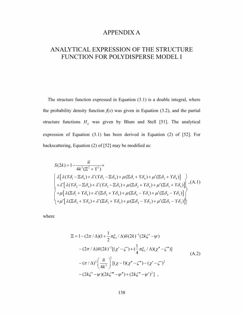
138
APPENDIX A
ANALYTICAL EXPRESSION OF THE STRUCTURE
FUNCTION FOR POLYDISPERSE MODEL I
The structure function expressed in Equation (3.1) is a double integral, where
the probability density function f(x) was given in Equation (3.2), and the partial
structure functions ijH was given by Blum and Stell [51]. The analytical
expression of Equation (3.1) has been derived in Equation (2) of [52]. For
backscattering, Equation (2) of [52] may be modified as:
3 2 2
1 6 2 4 1 6 2 4
2 4 3 5 2 4 3 5
1 6 2 4 6 1 4 2
2 4 3 5 4 2
(2 ) 14 ( )
( ) ( ) ( ) ( )
( ) ( ) ( ) ( )
( ) ( ) ( ) ( )
( ) ( ) ( )
nS k
k
5 3( )
, (A.1)
where
33
22
22 2
2
2
11 (2 / )(1 / ) (2 ) (2 )
21
(2 / ) (2 ) [( ) ( / )( )]4
( / ) [( 1)( ) ( )4
(2 )(2 ) (2 ) ] ,
n k k
n k
n
k
k k k
(A.2)

139
3 23
22
22
2
22
2
22
2
1(2 / )(1 / ) (2 ) ( 2 1)
21
(2 / ) (2 ) [2 ( / )(2 )]4
( / ) [(2 )( )]4
2( / ) (2 )( )4
( / ) (24
n k k
n k k k
nk
k
nk
k
nk
k
)( 1)] ,
(A.3)
and
1 3( / ){2 ( / )[ (2 )]}2
nk
k ,
22 ( / ) (2 )
2
nk
k ,
23 ( / ) (2 )
2
nk
k ,
4 ( / )[2 ( / ) ( )]2
nk
k ,
25 2( / ) [ ( 1) ]
2
nk
k ,
26 ( / ) ( )
2
n
k , (A.4)
and
bc ,

140
2 ( 1)b c c ,
3 ( 1)( 2)b c c c ,
/2 11 sin[ tan (2 )]cv c bk ,
( 1)/2 11 sin[( 1) tan (2 )]cbcv c bk ,
2 ( 2)/2 11( 1) sin[( 2) tan (2 )]cb c c v c bk ,
c/2 122 sin[ tan ( )]c v c bk ,
1 (c 1)/2 122 sin[( 1) tan ( )]c bcv c bk ,
c/2 11 cos[ tan (2 )]v c bk ,
( 1)/2 11 cos[( 1) tan (2 )]cbcv c bk ,
2 ( 2)/2 11( 1) cos[( 2) tan (2 )]cb c c v c bk ,
c/2 122 cos[ tan ( )]c v c bk ,
1 (c 1)/2 122 cos[( 1) tan ( )]c bcv c bk ,
2 11 [1 (2 ) ]v bk , 2 1
2 [4 (2 ) ]v bk , (A.5)
and

141
2
2 ( 1)nb c c , 3
3 ( 1)( 2)nb c c c , 31 / 6 ,
2 / ( 1)b a z , 1c z .
We would like to point out two typographic errors in the expression of in
Equation (2) of [52]. The expression of is correctly printed in Equation (A.2)
above. Also, we would like to point out that Equation (A.5) was modified from
Table I of [53] for backscattering.

142
APPENDIX B
ANALYTICAL EXPRESSION OF THE STRUCTURE FUNCTION FOR POLYDISPERSE MODEL II
We start from Equation (3.4) to derive the analytical expression of the structure
function for Polydisperse Model II derived from the fluid-filled sphere form
factor. The probability density function f(x) and the partial structure functions ijH
in Equation (3.4) were the same as those in Equation (3.1). The scattering
amplitude (2 )i k in Equation (3.4) takes the following form derived from the
fluid-filled sphere form factor:
(2 ) [sin(2 ) 2 cos(2 )]8
zi i i ik kx kx kx
k
, (B.1)
where 02( )z
Z Z
Z
, which describes the acoustic impedance contrast between
the sphere (Z) and the background (Z0). However, the acoustic impedance contrast
is irrelevant to Polydisperse Model II because 8
z
k
is a common factor between the
numerator and denominator of the fraction in Equation (3.4), and is cancelled out.
Calculating the double integral in Equation (3.4) gives the analytical expression
of (2 )S k for Polydisperse Model II as
(2 )
(2 ) 1(2 )
N
D
I kS k
I k , (B.2)

143
where
(2 ) ( ) /NI k k n ,
3 2 2
1 6 2 4 1 6 2 4
2 4 3 5 2 4 3 5
1 6 2 4 6 1 4 2
2 4 3 5
1(2 )
8 ( )
( ) ( ) ( ) ( )
( ) ( ) ( ) ( )
( ) ( ) ( ) ( )
( ) ( )
DI kk
4 2 5 3
,
( ) ( )
and
( ) ,
( ) ,
1 ,
.
k
k
k
k

144
REFERENCES
[1] C. F. Schueler, H. Lee, and G. Wade, “Fundamentals of digital ultrasonic processing,” IEEE Trans. Sonics Ultrason., vol. 31, no. 4, pp. 195–217, Jul. 1984.
[2] V. G. Murmis, J. J. Gisvold, T. M. Kinter, and J. F. Greenleaf, “Texture analysis of ultrasound B-scans to aid diagnosis of cancerous lesions in the breast,” in IEEE Ultrason. Symp. Proc., 1988, pp. 839–842.
[3] S. Krass, R. Brennecke, T. Voigtlaender, R. Kuprat, P. Staehr, H. J. Rupprecht, A. Fisch, H. Darius, and J. Meyer, “Tissue classification by texture and spectral analysis of intracoronary ultrasound radio-frequency data,” in Comput. Cardiol., 1988, pp. 641–643.
[4] F. M. J. Valckx and J. M. Thijssen, “Characterization of echographic image texture by cooccurrence matrix parameters,” Ultrasound Med. Biol., vol. 23, no. 4, pp. 559–571, 1997.
[5] F. L. Lizzi, M. Greenebaum, E. J. Feleppa, and M. Elbaurn, “Theoretical framework for spectrum analysis in ultrasonic tissue characterization,” J. Acoust. Soc. Am., vol. 73, no. 4, pp. 1366–1373, Apr. 1983.
[6] M. F. Insana, R. F. Wagner, D. G. Brown, and T. J. Hall, “Describing small-scale structure in random media using pulse-echo ultrasound,” J. Acoust. Soc. Am., vol. 87, no. 1, pp. 179–192, Jan. 1990.
[7] E. J. Feleppa, F. L. Lizzi, D. J. Coleman, and M. M. Yaremko, “Diagnostic spectrum analysis in ophthalmology: A physical perspective,” Ultrasound Med. Biol., vol. 12, no. 8, pp. 623–631, 1986.
[8] D. J. Coleman, R. H. Silverman, M. J. Rondeau, H. C. Boldt, H. O. Lloyd, F. L. Lizzi, T. A. Weingeist, X. Chen, S. Vangveeravong, and R. Folberg, “Noninvasive in vivo detection of prognostic indicators for high-risk uveal melanoma: Ultrasound parameter imaging,” Ophthalmology, vol. 111, no. 3, pp. 558–564, 2004.
[9] E. J. Feleppa, A. Kalisz, J. B. Sokil-Melgar, F. L. Lizzi, T. Liu, A. L. Rosado, M. C. Shao, W. R. Fair, Y. Wang, M. S. Cookson, V. E. Reuter, and W. D. W. Heston, “Typing of prostate tissue by ultrasonic spectrum analysis,” IEEE Trans. Ultrason. Ferroelectr. Freq. Control, vol. 43, no. 4, pp. 609–619, 1996.

145
[10] M. F. Insana, T. J. Hall, J. G. Wood, and Z. Y. Yan, “Renal ultrasound using parametric imaging techniques to detect changes in microstructure and function,” Invest. Radiol., vol. 28, no. 8, pp. 720–725, 1993.
[11] J. G. Miller, J. E. Perez, J. G. Mottley, E. I. Madaras, P. H. Johnston, E. D. Blodgett, L. J. Thomas, and B. E. Sobel, “Myocardial tissue characterization: An approach based on quantitative backscatter and attenuation,” in IEEE Ultrason. Symp. Proc, 1983, pp. 782–793.
[12] P. K. Tamirisa, M. R. Holland, J. G. Miller, and J. E. Perez, “Ultrasonic tissue characterization: Review of an approach to assess hypertrophic myocardium,” Echocardiography, vol. 18, no. 7, pp. 593–597, 2001.
[13] L. Y. L. Mo and R. S. C. Cobbold, “Theoretical models of ultrasonic scattering in blood,” in Ultrasonic Scattering in Biological Tissues, K. K. Shung and G. A. Thieme, Eds., Boca Raton, FL: CRC, 1993, ch. 5, pp. 125–170.
[14] F. T. H. Yu, E. Franceschini, B. Chayer, J. K. Armstrong, H. J. Meiselman, and G. Cloutier, “Ultrasonic parametric imaging of erythrocyte aggregation using the structure factor size estimator,” Biorheology, vol. 46, no. 4, pp. 343–363, 2009.
[15] E. Franceschini, B. Metzger, and G. Cloutier, “Forward problem study of an effective medium model for ultrasound blood characterization,” IEEE Trans. Ultrason. Ferroelect. Freq. Control, vol. 58, no. 12, pp. 2668–2679, 2012.
[16] E. Franceschini, R. K. Saha, and G. Cloutier, “Comparison of three scattering models for ultrasound blood characterization,” IEEE Trans. Ultrason. Ferroelect. Freq. Control, vol. 60, no. 11, pp. 2321–2334, 2013.
[17] M. L. Oelze, W. D. O’Brien, Jr., J. P. Blue, and J. F. Zachary, “Differentiation and characterization of rat mammary fibroadenomas and 4T1 mouse carcinomas using quantitative ultrasound imaging,” IEEE Trans. Med. Imag., vol. 23, no. 6, pp. 764–771, 2004.
[18] M. L. Oelze and W. D. O’Brien, Jr., “Application of three scattering models to characterization of solid tumors in mice,” Ultrason. Imaging, vol. 28, no. 2, pp. 83–96, 2006.
[19] M. L. Oelze and J. F. Zachary, “Examination of cancer in mouse models using high-frequency quantitative ultrasound,” Ultrasound Med. Biol., vol. 32, pp. 1639–1648, 2006.
[20] L. A. Wirtzfeld, K. Nam, Y. Labyed, G. Ghoshal, A. Haak, E. Sen-Gupta, Z. He, N. R. Hirtz, R. J. Miller, S. Sarwate, D. G. Simpson, J. A. Zagzebski, T. A. Bigelow, M. L. Oelze, T. J. Hall, and W. D. O'Brien Jr., “Techniques and

146
evaluation from a cross-platform imaging comparison of quantitative ultrasound parameters in an in vivo rodent fibroadenoma model,” IEEE Trans. Ultrason. Ferroelectr. Freq. Control, vol. 60, pp. 1386–1400, 2013.
[21] B. Garra, M. Insana, T. Shawker, R. F. Wagner, M. Bradford, and M. Russell, “Quantitative ultrasonic detection and classification of diffuse liver disease: Comparison with human observer performance,” Invest. Radiol., vol. 24, no. 3, pp. 196–203, 1989.
[22] M. P. Andre, A. Han, E. Heba, J. Hooker, R. Loomba, C. B. Sirlin, J. W. Erman, Jr., and W. D. O’Brien, Jr., “Accurate diagnosis of nonalcoholic fatty liver disease in human participants via quantitative ultrasound,” in IEEE Int. Ultrason. Symp. Proc., 2014, pp. 2375–2377.
[23] A. Han, J. W. Erdman, Jr., D. G. Simpson, M. P. Andre, and W. D. O’Brien, Jr., “Early detection of fatty liver disease in mice via quantitative ultrasound,” in IEEE Int. Ultrason. Symp. Proc., 2014, pp. 2363–2366.
[24] J. Mamou, A. Coron, M. L. Oelze, E. Saegusa-Beecroft, M. Hata, P. Lee, J. Machi, E. Yanagihara, P. Laugier, and E. J. Feleppa, “Three-dimensional high-frequency backscatter and envelope quantification of cancerous human lymph nodes,” Ultrasound Med. Biol., vol. 37, no. 3, pp. 345–357, 2011.
[25] M. C. Kolios, G. J. Czarnota, M. Lee, J. W. Hunt, and M. D. Sherar, “Ultrasonic spectral parameter characterization of apoptosis,” Ultrasound Med. Biol., vol. 28, no. 5, pp. 589–597, 2002.
[26] B. Banihashemi, R. Vlad, B. Debeljevic, A. Giles, M. C. Kolios, and G. J. Czarnota, “Ultrasound imaging of apoptosis in tumor response: Novel preclinical monitoring of photodynamic therapy effects,” Cancer Res., vol. 68, no. 20, pp. 8590–8596, 2008.
[27] R. M. Vlad, S. Brand, A. Giles, M. C. Kolios, and G. J. Czarnota, “Quantitative ultrasound characterization of responses to radiotherapy in cancer mouse models,” Clin. Cancer Res., vol. 15, no. 6, pp. 2067–2075, 2009.
[28] D. H. Turnbull, J. A. Ramsay, G. S. Shivji, T. S. Bloomfield, L. From, D. N. Sauder, and F. S. Foster, “Ultrasound backscatter microscope analysis of mouse melanoma progression,” Ultrasound Med. Biol., vol. 22, pp. 845–853, 1996.
[29] J. Mamou, M. L. Oelze, W. D. O’Brien Jr., and J. F. Zachary, “Identifying ultrasonic scattering sites from three-dimensional impedance maps,” J. Acoust. Soc. Am., vol. 117, pp. 413–423, 2005.
[30] A. J. Dapore, M. R. King, J. Harter, S. Sarwate, M. L. Oelze, J. A. Zagzebski, M. N. Do, T. J. Hall, and W. D. O'Brien, Jr., “Analysis of human fibroadenomas

147
using three-dimensional impedance maps,” IEEE Trans. Med. Imag., vol. 30, pp. 1206–1213, 2011.
[31] A. D. Pawlicki, A. J. Dapore, S. Sarwate, and W. D. O'Brien, Jr., “Three-dimensional impedance map analysis of rabbit liver,” J. Acoust. Soc. Am., vol. 130, pp. EL334–EL338, 2011.
[32] L. R. Taggart, R. E. Baddour, A. Giles, G. J. Czarnota, and M. C. Kolios, “Ultrasound characterization of whole cells and isolated nuclei,” Ultrasound Med. Biol., vol. 22, pp. 389–401, 2007.
[33] R. M. Vlad, R. K. Saha, N. M. Alajez, S. Ranieri, G. J. Czarnota, and M. C. Kolios, “An increase in cellular size variance contributes to the increase in ultrasound backscatter during cell death,” Ultrasound Med. Biol., vol. 36, no. 9, pp. 1546–1558, 2010.
[34] R. K. Saha, E. Franceschini, and G. Cloutier, “Assessment of accuracy of the structure-factor-size-estimator method in determining red blood cell aggregate size from ultrasound spectral backscatter coefficient,” J. Acoust. Soc. Am., vol. 129, no. 4, pp. 2269–2277, 2011.
[35] T. E. Doyle, A. T. Tew, K. H. Warnick, and B. L. Carruth, “Simulation of elastic wave scattering in cells and tissues at the microscopic level,” J. Acoust. Soc. Am., vol. 125, no. 3, pp. 1751–1767, 2009.
[36] M. Teisseire, A. Han, R. Abuhabsah, J. P. Blue, Jr., S. Sarwate, and W. D. O’Brien Jr., “Ultrasonic backscatter coefficient quantitative estimates from Chinese hamster ovary cell pellet biophantoms,” J. Acoust. Soc. Am., vol. 128, pp. 3175–3180, 2010.
[37] A. Han, R. Abuhabsah, J. P. Blue, Jr., S. Sarwate, and W. D. O'Brien, Jr., “Ultrasonic backscatter coefficient quantitative estimates from high-concentration Chinese hamster ovary cell pellet biophantoms,” J. Acoust. Soc. Am., vol. 130, pp. 4139–4147, 2011.
[38] V. C. Anderson, “Sound scattering from a fluid sphere,” J. Acoust. Soc. Am., vol. 22, pp. 426–431, 1950.
[39] J. J. Faran, “Sound scattering by solid cylinders and spheres,” J. Acoust. Soc. Am., vol. 23, pp. 405–418, 1951.
[40] J. McNew, R. Lavarello, and W. D. O’Brien Jr., “Sound scattering from two concentric fluid spheres,” J. Acoust. Soc. Am., vol. 125, pp. 1–4, 2009.
[41] V. Twersky, “Low-frequency scattering by correlated distributions of randomly oriented particles,” J. Acoust. Soc. Am., vol. 81, no. 5, pp. 1609–1618, 1987.

148
[42] L. S. Ornstein and F. Zernike, “Accidental deviations of density and opalescence at the critical point of a single substance,” Proc. Acad. Sci. Amsterdam, vol. 17, pp. 793–806, 1914.
[43] J. K. Percus and G. J. Yevick, “Analysis of classical statistical mechanics by means of collective coordinates,” Phys. Rev., vol. 110, pp. 1–13, 1958.
[44] D. Savery and G. Cloutier, “A point process approach to assess the frequency dependence of ultrasound backscattering by aggregating red blood cells,” J. Acoust. Soc. Am., vol. 110, pp. 3252–3262, 2001.
[45] F. T. H. Yu and G. Cloutier, “Experimental ultrasound characterization of red blood cell aggregation using the structure factor size estimator,” J. Acoust. Soc. Am., vol. 122, pp. 645–656, 2007.
[46] M. S. Wertheim, “Exact solution of the Percus-Yevick integral equation for hard spheres,” Phys. Rev. Lett., vol. 10, pp. 321–323, 1963.
[47] N. W. Ashcroft and J. Lekner, “Structure and resistivity of liquid metals,” Phys. Rev., vol. 145, no. 1, pp. 83–90, 1966.
[48] E. Franceschini and R. Guillermin, “Experimental assessment of four ultrasound scattering models for characterizing concentrated tissue-mimicking phantoms,” J. Acoust. Soc. Am., vol. 132, no. 6, pp. 3735–3747, 2012.
[49] V. Twersky, “Low-frequency scattering by mixtures of correlated nonspherical particles,” J. Acoust. Soc. Am., vol. 84, no. 1, pp. 409–415, 1988.
[50] R. K. Saha and M. C. Kolios, “Effects of cell spatial organization and size distribution on ultrasound backscattering,” IEEE Trans. Ultrason. Ferroelectr. Freq. Control, vol. 58, no. 10, pp. 2118–2131, 2011.
[51] L. Blum and G. Stell, “Polydisperse systems. I. Scattering function for polydisperse fluids of hard or permeable spheres,” J. Chem. Phys., vol. 71, pp. 42–46, 1979.
[52] W. L. Griffith, R. Triolo, and A. L. Compere, “Analytical structure function of a polydisperse Percus-Yevick fluid with Schulz (gamma) distributed diameters,” Phys. Rev. A., vol. 33, no. 3, pp. 2197–2200, 1986.
[53] W. L. Griffith, R. Triolo, and A. L. Compere, “Analytical scattering function of a polydisperse Percus-Yevick fluid with Schulz- (Γ-) distributed diameters,” Phys. Rev. A., vol. 35, no. 5, pp. 2200–2206, 1987.
[54] K. A. Wear, T. A. Stiles, G. R. Frank, E. L. Madsen, F. Cheng, E. J. Feleppa, C. S. Hall, B. S. Kim, P. Lee, W. D. O’Brien, Jr., M. L. Oelze, B. I. Raju, K. K.

149
Shung, T. A. Wilson, and J. R. Yuan, “Interlaboratory comparison of ultrasonic backscatter coefficient measurements from 2 to 9 MHz,” J. Ultrasound Med., vol. 24, no. 9, pp. 1235–1250, 2005.
[55] X. Chen, D. Phillips, K. Q. Schwarz, J. G. Mottley, and K. J. Parker, “The measurement of backscatter coefficient from a broadband pulse-echo system: A new formulation,” IEEE Trans. Ultrason. Ferroelectr. Freq. Control, vol. 44, pp. 515–525, 1997.
[56] A. S. Tunis, R. E. Baddour, G. J. Czarnota, A. Giles, A. E. Worthington, M. D. Sherar, and M. C. Kolios, “Using high frequency ultrasound envelope statistics to determine scatterer number density in dilute cell solutions,” in IEEE Ultrason. Symp. Proc, 2005, pp. 878–881.
[57] A. S. Tunis, G. J. Czarnota, A. Giles, M. D. Sherar, J. W. Hunt, and M. C. Kolios, “Monitoring structural changes in cells with high frequency ultrasound signal statistics,” Ultrasound Med. Biol., vol. 31, no. 8, pp. 1041–1049, 2005.
[58] L. A. Wirtzfeld, G. Ghoshal, I. M. Rosado-Mendez, K. Nam, Y. Park, A. D. Pawlicki1, R. J. Miller, D. G. Simpson, J. A. Zagzebski, M. L. Oelze, T. J. Hall, and W. D. O’Brien, Jr., “Quantitative ultrasound comparison of MAT and 4T1 mammary tumors in mice and rats across multiple imaging systems,” J. Ultrasound Med., accepted for publication, 2014.
[59] S. N. Chiu, D. Stoyan, W. S. Kendall, and J. Mecke, Stochastic Geometry and Its Applications, 3rd ed. Chichester, U.K. Wiley, 2013.
[60] J. C. Crocker and D. G. Grier, “Methods of digital video microscopy for colloidal studies,” J. Colloid Interface Sci., vol. 179, pp. 298–310, 1996.