1

Ultra Dense Small Cell Networks: Turning Densityinto Energy Efficiency

Sumudu Samarakoon, Student Member, IEEE, Mehdi Bennis, Senior Member, IEEE, WalidSaad, Senior Member, IEEE, Merouane Debbah, Fellow, IEEE and Matti Latva-aho, Senior Member, IEEE

Abstract—In this paper, a novel approach for joint powercontrol and user scheduling is proposed for optimizing energy ef-ficiency (EE), in terms of bits per unit energy, in ultra dense smallcell networks (UDNs). Due to severe coupling in interference,this problem is formulated as a dynamic stochastic game (DSG)between small cell base stations (SBSs). This game enables tocapture the dynamics of both the queues and channel states of thesystem. To solve this game, assuming a large homogeneous UDNdeployment, the problem is cast as a mean-field game (MFG)in which the MFG equilibrium is analyzed with the aid of low-complexity tractable partial differential equations. Exploiting thestochastic nature of the problem, user scheduling is formulatedas a stochastic optimization problem and solved using the driftplus penalty (DPP) approach in the framework of Lyapunovoptimization. Remarkably, it is shown that by weaving notionsfrom Lyapunov optimization and mean-field theory, the proposedsolution yields an equilibrium control policy per SBS whichmaximizes the network utility while ensuring users’ quality-of-service. Simulation results show that the proposed approachachieves up to 70.7% gains in EE and 99.5% reductions in thenetwork’s outage probabilities compared to a baseline modelwhich focuses on improving EE while attempting to satisfy theusers’ instantaneous quality-of-service requirements.

Index Terms—Dynamic stochastic game, Lyapunov optimiza-tion, mean field games, ultra dense network, 5G

I. INTRODUCTION

Wireless network densification is viewed as a promisingapproach to enable a 1000x improvement in wireless cellularnetwork capacity [1]–[4]. Indeed, 5G systems are expected tobe ultra-dense in terms of transmitters and receivers renderingnetwork optimization highly complex [2] and [5]. In such ultradense network (UDN) environments, resource managementproblems, such as power control and user equipment (UE)scheduling, become significantly more challenging due to thescale of the network [2], [6]. In addition, the spatio-temporaltraffic demand fluctuations in the network, the dynamics inchannel conditions, and the increasing overhead due to the

This work is supported by the TEKES grant 2364/31/2014, the Academyof Finland (289611), the 5Gto10G project, the SHARING project underthe Finland grant 128010, the U.S. National Science Foundation (NSF)under Grants CNS-1460333, CNS-1460316, and CNS-1513697, and the ERCStarting Grant 305123 MORE (Advanced Mathematical Tools for ComplexNetwork Engineering).

S. Samarakoon, M. Bennis and M. Latva-aho are with the Depart-ment of Communications Engineering, University of Oulu, Finland (e-mail:{sumudu,bennis,matti.latva-aho}@ee.oulu.fi).

W. Saad is with Wireless@VT, Bradley Department of Electrical and Com-puter Engineering, Virginia Tech, Blacksburg, VA (email: walids@vt.edu).

M. Debbah is with Mathematical and Algorithmic Sciences Lab, HuaweiFrance R&D, Paris, France, (email: merouane.debbah@huawei.fr) and withthe Large Systems and Networks Group (LANEAS), CentraleSupelec, Uni-versite Paris-Saclay, 3 rue Joliot-Curie, 91192 Gif-sur-Yvette, France.

need for coordination will further exacerbate the challenges ofresource management in UDNs. For instance, the uncertaintiesin terms of queue state information (QSI) and channel stateinformation (CSI) as well as their evolution over time willplay a pivotal role in resource optimization.

Due to the involvement of large number of devices andthe severe coupling of their control parameters with one an-other, the current state-of-the-art approaches used in classical,small scale network deployments are inadequate to studythe resource optimization in UDNs. Thus, power control,UE scheduling, interference mitigation, and base station (BS)deployment strategies for energy-efficient UDN have beenrecently investigated in a number of works such as [1] and[5]–[11]. The work in [6] investigates the potential gainsand limitations of energy efficiency (EE) for outdoor UDNsconsidering small cells idle mode capabilities and BS/UEdensification. In [7], an analytical framework was proposed fordesigning UDNs that maximizes EE by modeling the networkusing stochastic geometry and obtaining new lower bound onthe average spectral efficiency. The authors in [8] investigatehow different BS and antenna deployment strategies, for bothindoor and outdoor UDNs, can impact EE. In [9], a powercontrol and UE scheduling mechanism is proposed for UDNof clustered small cells which have access to a databaseconsisting signal-to-noise ratio values of each BS-UE link.The work in [10] proposes an optimization framework whichallows flexible UE association among densely deployed BSsby minimizing the signaling overhead. The authors in [11]study how to improve EE of an UDN by jointly optimizingthe resource utilization and the temporal variances in thetraffic load. These studies provide valuable insights of bothperformance gains and limitations of UDNs. However, mostof these works [6]–[10], ignore uncertainties in QSI, do notproperly model network dynamics, and typically focus onthe problems of UE scheduling and resource allocation inisolation. Instead, in practice, there is a need to treat thoseproblems jointly while accounting for the QSI dynamics anduncertainty. Moreover, none of these existing works study thebehavior of the ultra dense system setting in which the numberof BSs and UEs grows infinitely large.

Recently, mean-field games (MFGs) received significantattention in the context of cellular networks with large numberof players [12]–[16]. In MFGs, a large population consistsof small interacting individual players and their decisionmaking strategies are studied [12], [13]. Due to the size ofthe population, the impacts of individual states and decisionsare negligible while the abstract behavior of the population is

arX

iv:1

603.

0368

2v2

[cs

.NI]

14

Mar

201

6

2

modeled by a mean-field (MF). As a result, the MF regimeallows to cast the multi-player problem into a more tractablesingle player problem which depends on the state distributionof the population. In [14], concurrent packet transmissionsamong large number of transmitter-receiver pairs with theobjective of minimizing transmit power under the uncertaintiesof QSI and CSI are investigated using MFGs. The authorsin [15] study an energy efficient power control problem in mul-tiple access channels whereas transmitters strategies dependon their receivers, battery levels and the strategies of others.In [16], a competition of wireless resource sharing amonglarge number of agents is investigated as an MFG. Despitetheir interesting analytical perspective, these existing worksremain limited to traditional macrocellular networks and donot address the challenges of small cell networks. Moreover,for simplicity, these works consider models with a single UEper BS or they address multi-user scenarios with conventionalUE scheduling schemes (proportional-fair, round-robin, first-in-first-out). Thus, the opportunity to improve the proposedsolutions for multi-user cases by smart UE scheduling has notbeen treated yet.

When considering multiple UEs associated with SBS, UEscheduling directly affects the performance of each SBS. Dueto the dynamic nature of channels and arbitrary arrivals, theUE scheduling process becomes a stochastic optimizationproblem [17]–[20]. To solve such stochastic optimizationproblems while ensuring queue stability, the dual-plus-penalty(DPP) theorem from the Lyapunov optimization frameworkcan be used [17]–[22]. Lyapunov DPP approach simplifiesthe stochastic optimization problem into multiple subproblemswhich can be solved at each time instance. Remarkably, thissimplification ensures the convergence to the optimal solutionof the original stochastic optimization problem [17]–[20]. Thework in [19] presents a utility optimal scheduling algorithmfor processing networks based on Lyapunov DPP approach.In [21], Lyapunov DPP method is used to solve stochasticoptimization problem with non-convex objective functions.In [22], a Lyapunov DPP framework is used to dynamicallyselect service nodes for multiple video streaming UEs in awireless network. It can be noted that the Lyapunov DPPapproach is a powerful tool for solving stochastic optimizationproblems. However, to implement the above technique indecentralized control mechanisms, i) the objective functionshould be chosen such that it can be decoupled among thecontrol nodes as in [19] or ii) necessary bounds need to beidentified for the coupling term as the authors in [22] evaluatea lower bound for the capacity in order to mitigate couplingdue to interference. Therefore, a suitable method to makean accurate evaluation on the coupled term (interference inwireless UDNs) needs to be investigated.

The main contribution of this paper is to propose a noveljoint power control and user scheduling mechanism for ultra-dense small cell networks with large number of small cell basestations (SBSs). In the studied model, the objective of SBSsis to maximize their own time average energy efficiency (EE)in terms of the amount of bits transmitted per joule of energyconsumption. Due to the ultra-dense deployment, severe mu-tual interference is experienced by all SBSs and thus, must be

properly managed. To this end, SBSs have to compete withone another in order to maximize their EEs while ensuringUEs’ quality-of-service (QoS). This competition is cast as adynamic stochastic game (DSG) in which players are the SBSsand their actions are their control vectors which determine thetransmit power and user scheduling policy. Due to the non-tractability of the DSG, we study the problem in the mean-fieldregime which enables us to capture a very dense small celldeployment. Thus, employing a homogeneous control policyamong all the SBSs in the network, the solution of the DSGis obtained by solving a set of coupled partial differentialequations (PDEs) known as Hamilton-Jacobi-Bellman (HJB)and Fokker-Planck-Kolmogorov (FPK) equations [12]. Theresulting equilibrium is known as the mean-field equilibrium(MFE). We analyze the sufficient conditions for the existenceof an MFE in our problem and we prove that all SBSsconverge to this MFE. Exploiting the stochastic nature of theobjective with respect to QSI and CSI, the UE schedulingprocedure is modeled as a stochastic optimization problem.To ensure the queue stability and thus, UE’s QoS, the UEscheduling problem is solved within a DPP-based Lyapunovoptimization framework [17], [22]. An algorithm is proposedin which each SBS schedules its UEs as a function of CSI,QSI and the mean-field of interferers. Remarkably, it is shownthat combining the power allocation policy obtained from theMFG and the DPP-based scheduling policy enables SBSs toautonomously determine their optimal transmission parameterswithout coordination with other neighboring cells. To the bestof our knowledge, this is the first work combining MFG andLyapunov frameworks within the scope of UDNs. Simulationresults show that the proposed approach achieves up to 70.7%gains in EE and 99.5% reductions in the network’s outageprobabilities compared to a baseline model which improvesEE while satisfying users’ instantaneous quality-of-servicerequirements.

The rest of this paper is organized as follows. Section IIpresents the system model, formulates the DSG with finitenumber of players and discusses the sufficient conditions toobtain an equilibrium for the DSG. In Section III, using theassumptions of large number of players the DSG is cast asa MFG and solved. The solution for UE scheduling at eachSBS based on DPP framework is examined in Section IV. Theresults are discussed in Section V and finally, conclusions aredrawn in Section VI.

II. SYSTEM MODEL AND PROBLEM DEFINITION

Consider a downlink of an ultra dense wireless small cellnetwork that consists of a set of B SBSs B using a commonspectrum with bandwidth ω. These SBSs serve a set M ofM UEs. Here, M = M1 ∪ · · · ∪ MB where Mb is the setof UEs served by SBS b ∈ B. For UE scheduling, we use ascheduling vector λb(t) =

[λbm(t)

]∀m∈Mb

for SBS b whereλbm(t) = 1 indicates that UE m ∈Mb is served by SBS b attime t and λbm(t) = 0 otherwise. The channel gain betweenUE m ∈Mb and SBS b at time t is denoted by hbm(t) and anadditive white Gaussian noise with zero mean and σ2 variance

3

is assumed. The instantaneous data rate of UE m is given by:

rbm(t) = ωλbm(t) log2

(1 +

pb(t)|hbm(t)|2Ibm(t) + σ2

), (1)

where pb(t) ∈ [0, pmaxb ] is the transmission power of SBS

b, |hbm(t)|2 is the channel gain between SBS b and UE m,Ibm(t) =

∑∀b′∈B\{b} pb′(t)|hb′m(t)|2 is the interference term.

We assume that SBS b sends qbm(t) bits to UE m ∈ Mb.Thus, the time evolution of the b-th SBS queue, is given by:

dqb(t) = ab(t)− rb(t,Y (t),h(t)

)dt, (2)

where ab(t) and rb(·) are the vectors of arrivals and transmis-sion rates at SBS b and is the vector of channel gains. More-over, a vector of control variables Y (t) =

[yb(t),y−b(t)

]

is defined such that yb(t) =[λb(t), pb(t)

]is the SBS local

control vector and y−b(t) is the control vector of interferingSBSs. The evolution of the channels are assumed to varyaccording to the following known stochastic model [23]:

dhb(t) = G(t,hb(t)

)dt+ ζdzb(t), (3)

where the deterministic part hb(t))

= [G(t, hbm(t)

)]m∈M

considers path loss and shadowing while the random partzb(t) = [zbm(t)]m∈M with positive constant ζ includes fastfading and channel uncertainties. The evolution of the entiresystem can be described by the QSI and the CSI as per (2) and(3), respectively. Thus, we define x(t) =

[xb(t)

]b∈B ∈ X as

the state of the system at time t with xb(t) =[qb(t),hb(t)

]

over the state space X = (X1 ∪ · · · ∪ XB). The feasibility setof SBS b’s control at state x(t) is defined as Yb

(t,x(t)

)=

{λbm(t,x(t)

)∈ {0, 1}, 0 ≤ pb

(t,x(t)

)≤ p

max}. Note thatwe will frequently use Y (t) instead Y

(t,x(t)

)for notational

simplicity. As the system evolves, UEs need to be scheduledat each time slot based on QSI and CSI. The service qualityof UE is ensured such that the average queue of packetsintended for UE m ∈ Mb at its serving SBS b is finite, i.e.qbm = limt→∞

1t

∑t−1τ=0 qbm(τ) ≤ ∞.

The objective of this work is to determine the con-trol policy per SBS b which maximizes a utility func-tion fb(·) while ensuring UEs’ quality of service (QoS).The utility of a SBS at time t is its EE which is de-fined as 1†rb

(t,Y (t),h(t)

)/(pb(t) + p0). Here, p0 is the

fixed circuit power consumption at an SBS [24]. Let Y =limt→∞

1t

∑t−1τ=0 Y (τ) be the limiting time average expec-

tation of the control variables Y (t). Formally, the utilitymaximization problem for SBS b can be written as:

maximizeyb

fb(yb, y−b), (4a)

subject to qbm ≤ ∞ ∀m ∈Mb, (4b)(2), (3), (4c)yb(t) ∈ Yb(t,x) ∀t. (4d)

Furthermore, we assume that SBSs serve their scheduledUEs for a time period of T . Therefore, we use the notionof time scale separation between transmit power allocationand UE scheduling processes, hereinafter. For SBS b ∈ B,the transmit power allocation pb(t) is determined for eachtransmission and thus, is a fast process. However, UE schedul-ing λb(t) is fixed for a duration of T to ensure a stable

transmission. Therefore, UE scheduling is a slower processthan power allocation.

A. Resource management as a dynamic stochastic game

We focus on finding a control policy which solves (4) over atime period [0, T ] for a given set of scheduled UEs consideringthe state transitions x(0) → x(T ). Therefore, we define thefollowing time-and-state-based utility for SBS b:

Γb(0,x(0)

)= Γb

(0,x(0),Y (0)

)

= E[ ∫ T

0

fb(τ,x(τ),Y (τ)

)dτ]. (5)

The goal of each SBS is to maximize this utility over yb(τ) =[λ?b(τ), pb(τ)

]for a given UE scheduling λ?(τ) subject to

the system state dynamics dx(t) = Xtdt + Xzdz(t), ∀b ∈B,∀m ∈M where:

Xt =[abm(t)− rbm

(t,Y (t),h(t)

), G(t, hbm(t)

)]m∈M,b∈B

,

and Xz = diag(0|M|, ζ1).As the network state evolves as a function of QSI and

CSI, the strategies of the SBSs must adapt accordingly. Thus,maximizing the utility Γb

(0,x(0)

)for b ∈ B under the

evolution of the network states can be modeled as a dynamicstochastic game (DSG) as follows:

Definition 1: For a given UE scheduling mechanism, thepower control problem can be formulated as a dynamicstochastic game G = (B, {Yb}b∈B, {Xb}b∈B, {Γb}b∈B) where:• B is the set of players which are the SBSs.• Yb is the set of actions of player b ∈ B which encompass

the choices of transmit power pb for given scheduled UEsλb.

• Xb is the state space of player b ∈ B consisting QSI qband CSI hb.

• Γb is the average utility of player b ∈ B that depends onthe state transition x(t)→ x(T ) as follows:

Γb(t,x(t)

)= E

[ ∫ Ttfb(τ,x(τ),Y (τ)

)dτ]. (6)

One suitable solution for the defined DSG is the closed-loopNash equilibrium (CLNE) defined as follows:

Definition 2: The control variables Y ?(t) =(y?b(t),y

?−b(t)

)∈ Y

(t,x(t)

)constitute a closed-loop

Nash equilibrium if, for Y(t,x(t)

)=(Y1

(t,x(t)

)∪ · · · ∪

Y|B|(t,x(t)

)),

E[ ∫ Ttfb(τ,x(τ),y?b(τ),y?−b(τ)

)dτ]

≥ E[ ∫ Ttfb(τ,x(τ),yb(τ),y?−b(τ)

)dτ], (7)

is satisfied ∀ b ∈ B, ∀ Y (t) ∈ Y(t,x(t)

)and ∀ x(t) ∈ X .

To satisfy (7), each SBS must have the knowledge of its ownstate xb(t) and a feedback on the optimal strategy y?−b(t) ofthe rest of SBSs and thus, the achieved equilibrium is knownas a CLNE. We denote by Γ?

(t,x(t)

)=[Γ?b(t,x(t)

)]b∈B the

trajectories of the utilities induced by the NE. The existenceof the NE is ensured by the existence of a joint solution

4

Γ(t,x(t)

)=[Γb(t,x(t)

)]∀b∈B to the following |B| coupled

HJB equations [12]:

∂∂t [Γb

(t,x(t)

)] + max

yb(t,x(t))

[Xt

∂∂x [Γb

(t,x(t)

)]

+ fb(t,x(t),Y (t))

+ 12 tr(X2z∂2

∂x2 [Γb(t,x(t)

)])]

= 0, (8)

defined for each SBS b ∈ B and tr(·) is the matrix traceoperation.

Proposition 1: (Existence of a closed-loop NE in G) Asufficient condition for the existence of a closed-loop NE in Gis that for all (v?, p?), we must have 2v?(p? + p0) + β ln(1 +

βp?) 6= 0 where β = |hbm(t)2|Ibm(t)+σ2 for all b ∈ B and their

scheduled UEs m ∈M.Proof: Proving the existence of a solution to the HJB

equation given in (8) each SBS provides a sufficient conditionfor the existence of a NE for the DSG [12]. Thus, there existsa solution if the function

F(x(t),y−b(t),

∂[Γb(t,x(t))]∂qb

)= maxyb(t,x(t))

[fb((t,x(t),Y (t)

)

− rbm(t,x(t),Y (t))∂[Γb(t,x(t))]

∂qb

], (9)

is smooth [25]. According to (6), the average utilityΓb (t,x(t)) that depends on the state transition x(t) →x(T ) is independent of the current choice of controls yb(t).Therefore, the terms ∂[Γb(t,x(t))]

∂qb, ∂[Γb(t,x(t))]

∂hband ∂2[Γb(t,x(t))]

∂h2b

become constant with respect to yb(t) and thus, are neglectedsince they do not impact on F (·). Considering the firstderivative, the maximizer needs to satisfy ∂fb

∂yyb− ∂rb∂yb

∂Γb

∂qb= 0

which yields,

v(p+ p0)2 = β(p+ p0)− (1 + βp) log(1 + βp), (10)

where p is the transmit power of the respective SBS and v =∂Γb

∂qbβ. Note that we have omitted the dependencies over time

and states for notational simplicity.In order to evaluate the smoothness of

F(x(t),y−b(t),

∂[Γb(t,x(t))]∂qb

), we use the implicit

function theorem [26]. Thus, we define a functionF(v, p) = v(p + p0)2 − β(p + p0) + (1 + βp) log(1 + βp)and check whether F(v, p) = 0 is held. If F(v, p) = 0is held, there exists ϕ : < → < such that p? = ϕ(v?)

and ∂[ϕ(v?)]∂v = ∂[F(v?,p?)]

∂v /∂[F(v?,p?)]∂p < ∞. Since

∂[ϕ(v?)]∂v = (p?+p0)2

2v?(p?+p0)+β ln(1+βp?) , the smoothness isensured by

2v?(p? + p0) + β ln(1 + βp?) 6= 0. (11)

Note that we consider ∂Γb

∂qb> 0 and thus, v > 0 and v is

bounded above, i.e. 0 < v < ∞. A bounded v ensures thesolution to (10) remains finite (finite transmit power) whilev > 0 guarantees 2v?(p? + p0) + β ln(1 + βp?) > 0 for allfeasible transmit powers. Thus, the above sufficient condition(11) is held for all the particular choices of v and p.

Solving |B| mutually coupled HJB equations is complexwhen |B| > 2. Furthermore, it requires gathering QSI andCSI from all the SBSs throughout the network which incurs

a tremendous amount of information exchange. Hence, itis impractical for UDNs with large |B|. However, as |B|grows extremely large, it can be observed that the set ofall players transform into a continuum and their individualitybecomes indistinguishable. In such a scenario, we can solvethe dynamic stochastic game using the tools of mean-fieldtheory, as explained next.

III. OPTIMAL POWER CONTROL: A MEAN-FIELDAPPROACH

As the number of SBSs becomes large (|B| → ∞), weassume that the interference tends to be bounded in orderto have non-zero rates as observed in [14], [15] and [27].Moreover, each SBS implements a transmission policy basedon the knowledge of its own state. SBSs in such an environ-ment are indistinguishable from one another thus, resultingin a continuum of players. This is a reasonable assumptionin UDNs because the impact of an individual SBS’s decisionon the system is negligible from the macroscopic view unlesssuch a decision is adopted by a considerable large portion ofthe population. As an example, the choice of a SBS to increaseits energy consumption by 1 Watt in a system consistingof thousands of SBSs consuming couple of megawatts isinsignificant. However, it is a significant increment of energyconsumption if the same decision is made by 10% of thepopulation together. Remarkably, increasing the number ofSBSs infinitely large and allow them to become a continuumallows us to simplify the solution of all |B| HJB equations byreducing them to two equations as discussed below.

At a given time and state(t,x(t)

)and for a scheduled UE

m, the impact of other SBSs on the choice of a given SBSb ∈ B appears in the interference term:

Ibm(t,x(t)

)=∑∀b′∈B\{b} pb′

(t,x(t)

)|hb′m(t)|2.

As the number of SBSs grows large, we consider that the in-terference is bounded as shown in [27]–[29] and [30] since thepath loss is modeled according to the inverse-square law. Thus,the interference term can be rewritten by using a normalizationfactor for the channels [27]. Let η/|B| be the normalizationfactor where η is SBS density and thus, the channel gainbecomes hbm(t) =

√ηhbm(t)√|B|

with E [|hbm(t)|2] = 1. Thus,

the interference can be rewritten as (12) with a SBS statedistribution ρ|B|(t) = [ρ|B|

(t,x′)]x′∈X where

ρ|B|(t,x′) =

1

|B||B|∑b=1

δ(xb(t) = x′

). (13)

Here, δ(·) is the Dirac delta function and x′ ∈ X .Now, we assume that each SBS has only the knowledge

of its own state and, thus, it will implement a homogeneoustransmission policy, i.e. pb

(t,x(t)

)= p

(t,xb(t)

)for all b ∈

B, based the knowledge that it has available. Furthermore,the transmission policy satisfies E [

∫ T0p2(t,xb(t)

)dt] < ∞.

With the above assumptions, the SBS states x1(t), . . . ,x|B|(t)for all t become exchangeable under the transmission policyp [31], [32], i.e.,

L(x1(t), . . . ,x|B|(t)

)= L

(xπ(1), . . . ,xπ(|B|)

)for p, ∀t,

(14)

5

Ibm(t,x(t)

)=

η

|B|∑

∀b′∈B\{b}

pb′(t,x(t)

)|x(t)|2 =

η

|B|∑

∀b′∈B

pb′(t,x(t)

)|x(t)|2 − η

|B|pb(t,x(t)

)|hbm(t)|2

= η

∫

Xpb′(t,xb′)|hb′m|2ρ|B|(t,xb′)dxb′ −

η

|B|pb(t,x(t)

)|hbm(t)|2.

(12)

UE m

BS b

Mean field InterferenceIm

(t,ρ(t)

)

Ab(t)qb(t)

pb(t), λb(t)

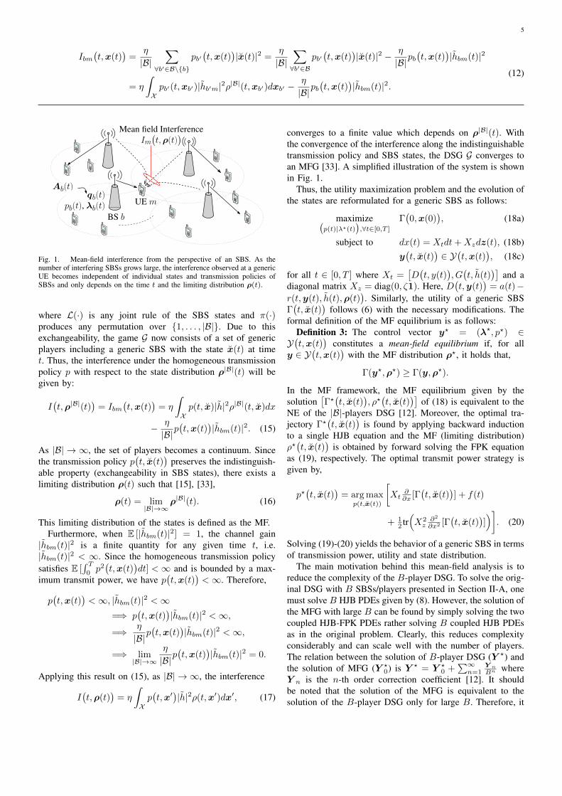
Fig. 1. Mean-field interference from the perspective of an SBS. As thenumber of interfering SBSs grows large, the interference observed at a genericUE becomes independent of individual states and transmission policies ofSBSs and only depends on the time t and the limiting distribution ρ(t).

where L(·) is any joint rule of the SBS states and π(·)produces any permutation over {1, . . . , |B|}. Due to thisexchangeability, the game G now consists of a set of genericplayers including a generic SBS with the state x(t) at timet. Thus, the interference under the homogeneous transmissionpolicy p with respect to the state distribution ρ|B|(t) will begiven by:

I(t,ρ|B|(t)

)= Ibm

(t,x(t)

)= η

∫

Xp(t, x)|h|2ρ|B|(t, x)dx

− η

|B|p(t,x(t)

)|hbm(t)|2. (15)

As |B| → ∞, the set of players becomes a continuum. Sincethe transmission policy p

(t, x(t)

)preserves the indistinguish-

able property (exchangeability in SBS states), there exists alimiting distribution ρ(t) such that [15], [33],

ρ(t) = lim|B|→∞

ρ|B|(t). (16)

This limiting distribution of the states is defined as the MF.Furthermore, when E [|hbm(t)|2] = 1, the channel gain

|hbm(t)|2 is a finite quantity for any given time t, i.e.|hbm(t)|2 < ∞. Since the homogeneous transmission policysatisfies E [

∫ T0p2(t,x(t)

)dt] <∞ and is bounded by a max-

imum transmit power, we have p(t,x(t)

)<∞. Therefore,

p(t,x(t)

)<∞, |hbm(t)|2 <∞

=⇒ p(t,x(t)

)|hbm(t)|2 <∞,

=⇒ η

|B|p(t,x(t)

)|hbm(t)|2 <∞,

=⇒ lim|B|→∞

η

|B|p(t,x(t)

)|hbm(t)|2 = 0.

Applying this result on (15), as |B| → ∞, the interference

I(t,ρ(t)

)= η

∫

Xp(t,x′

)|h|2ρ(t,x′)dx′, (17)

converges to a finite value which depends on ρ|B|(t). Withthe convergence of the interference along the indistinguishabletransmission policy and SBS states, the DSG G converges toan MFG [33]. A simplified illustration of the system is shownin Fig. 1.

Thus, the utility maximization problem and the evolution ofthe states are reformulated for a generic SBS as follows:

maximize(p(t)|λ?(t)

),∀t∈[0,T ]

Γ(0,x(0)

), (18a)

subject to dx(t) = Xtdt+Xzdz(t), (18b)y(t, x(t)

)∈ Y

(t,x(t)

), (18c)

for all t ∈ [0, T ] where Xt =[D(t, y(t)

), G(t, h(t)

)]and a

diagonal matrix Xz = diag(0, ζ1). Here, D(t,y(t)

)= a(t)−

r(t,y(t), h(t),ρ(t)). Similarly, the utility of a generic SBS

Γ(t, x(t)

)follows (6) with the necessary modifications. The

formal definition of the MF equilibrium is as follows:Definition 3: The control vector y? = (λ?, p?) ∈Y(t,x(t)

)constitutes a mean-field equilibrium if, for all

y ∈ Y(t,x(t)

)with the MF distribution ρ?, it holds that,

Γ(y?,ρ?) ≥ Γ(y,ρ?).

In the MF framework, the MF equilibrium given by thesolution

[Γ?(t, x(t)

), ρ?(t, x(t)

)]of (18) is equivalent to the

NE of the |B|-players DSG [12]. Moreover, the optimal tra-jectory Γ?

(t, x(t)

)is found by applying backward induction

to a single HJB equation and the MF (limiting distribution)ρ?(t, x(t)

)is obtained by forward solving the FPK equation

as (19), respectively. The optimal transmit power strategy isgiven by,

p?(t, x(t)

)= arg max

p(t,x(t))

[Xt

∂∂x [Γ

(t, x(t)

)] + f(t)

+ 12 tr(X2z∂2

∂x2 [Γ(t, x(t)

)])]. (20)

Solving (19)-(20) yields the behavior of a generic SBS in termsof transmission power, utility and state distribution.

The main motivation behind this mean-field analysis is toreduce the complexity of the B-player DSG. To solve the orig-inal DSG with B SBSs/players presented in Section II-A, onemust solve B HJB PDEs given by (8). However, the solution ofthe MFG with large B can be found by simply solving the twocoupled HJB-FPK PDEs rather solving B coupled HJB PDEsas in the original problem. Clearly, this reduces complexityconsiderably and can scale well with the number of players.The relation between the solution of B-player DSG (Y ?) andthe solution of MFG (Y ?

0) is Y ? = Y ?0 +

∑∞n=1

Y n

Bn whereY n is the n-th order correction coefficient [12]. It shouldbe noted that the solution of the MFG is equivalent to thesolution of the B-player DSG only for large B. Therefore, it

6

∂∂t [Γ

(t, x(t)

)] + max

p(t,x(t))

[D(t,y?(t)

)∂∂q [Γ

(t, x(t)

)] + f(t) +

(G(t, h) ∂

∂h+ ζ2

2∂2

∂h2

)Γ(t, x(t)

)]= 0,

∂∂h

[G(t, h)ρ

(t, x(t)

)]− ζ2

2∂2

∂h2[ρ(t, x(t)

)] + ∂

∂q

[D(t,y?(t)

)ρ(t, x(t)

)]+ ∂tρ

(t, x(t)

)= 0,

(19)

0 100 200 300 400 500 600 700 800 9000

20

40

60

80

100

Number of SBSs

Itera

tio

ns

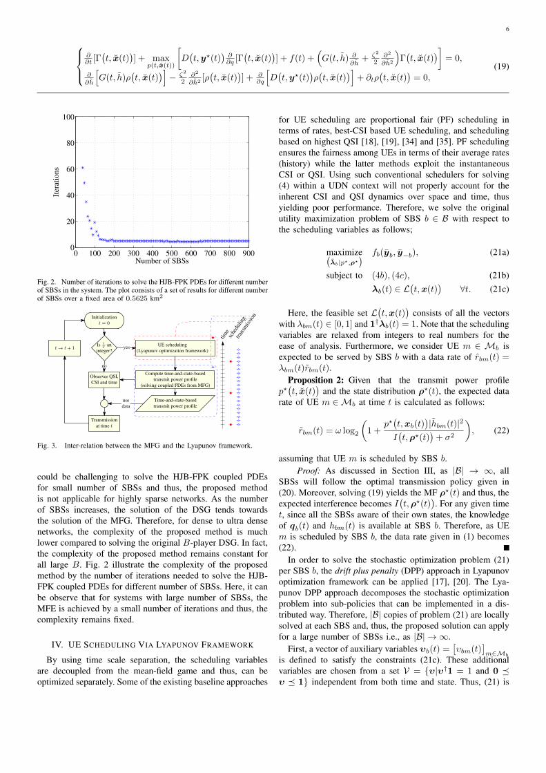
Fig. 2. Number of iterations to solve the HJB-FPK PDEs for different numberof SBSs in the system. The plot consists of a set of results for different numberof SBSs over a fixed area of 0.5625 km2

Initializationt = 0

Is tT an

integer?

Compute time-and-state-basedtransmit power profile

(solving coupled PDEs from MFG)

Observer QSI,CSI and time

t → t+ 1

Time-and-state-basedtransmit power profile

Transmissionat time t

yes

no

usedata

UE scheduling(Lyapunov optimization framework)

time

sche

dulin

gtra

nsm

issio

n

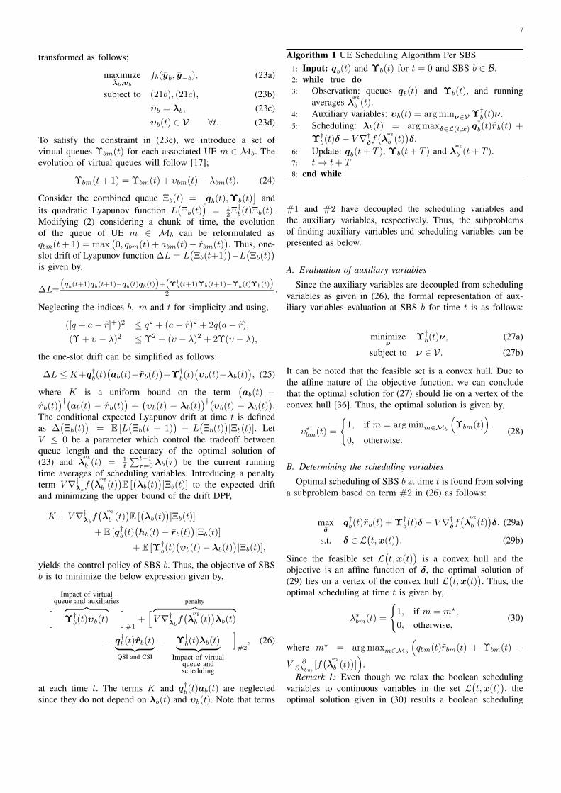
Fig. 3. Inter-relation between the MFG and the Lyapunov framework.

could be challenging to solve the HJB-FPK coupled PDEsfor small number of SBSs and thus, the proposed methodis not applicable for highly sparse networks. As the numberof SBSs increases, the solution of the DSG tends towardsthe solution of the MFG. Therefore, for dense to ultra densenetworks, the complexity of the proposed method is muchlower compared to solving the original B-player DSG. In fact,the complexity of the proposed method remains constant forall large B. Fig. 2 illustrate the complexity of the proposedmethod by the number of iterations needed to solve the HJB-FPK coupled PDEs for different number of SBSs. Here, it canbe observe that for systems with large number of SBSs, theMFE is achieved by a small number of iterations and thus, thecomplexity remains fixed.

IV. UE SCHEDULING VIA LYAPUNOV FRAMEWORK

By using time scale separation, the scheduling variablesare decoupled from the mean-field game and thus, can beoptimized separately. Some of the existing baseline approaches

for UE scheduling are proportional fair (PF) scheduling interms of rates, best-CSI based UE scheduling, and schedulingbased on highest QSI [18], [19], [34] and [35]. PF schedulingensures the fairness among UEs in terms of their average rates(history) while the latter methods exploit the instantaneousCSI or QSI. Using such conventional schedulers for solving(4) within a UDN context will not properly account for theinherent CSI and QSI dynamics over space and time, thusyielding poor performance. Therefore, we solve the originalutility maximization problem of SBS b ∈ B with respect tothe scheduling variables as follows;

maximize(λb|p?,ρ?

) fb(yb, y−b), (21a)

subject to (4b), (4c), (21b)λb(t) ∈ L

(t,x(t)

)∀t. (21c)

Here, the feasible set L(t,x(t)

)consists of all the vectors

with λbm(t) ∈ [0, 1] and 1†λb(t) = 1. Note that the schedulingvariables are relaxed from integers to real numbers for theease of analysis. Furthermore, we consider UE m ∈ Mb isexpected to be served by SBS b with a data rate of rbm(t) =λbm(t)rbm(t).

Proposition 2: Given that the transmit power profilep?(t, x(t)

)and the state distribution ρ?(t), the expected data

rate of UE m ∈Mb at time t is calculated as follows:

rbm(t) = ω log2

(1 +

p?(t,xb(t)

)|hbm(t)|2

I(t,ρ?(t)

)+ σ2

), (22)

assuming that UE m is scheduled by SBS b.Proof: As discussed in Section III, as |B| → ∞, all

SBSs will follow the optimal transmission policy given in(20). Moreover, solving (19) yields the MF ρ?(t) and thus, theexpected interference becomes I

(t,ρ?(t)

). For any given time

t, since all the SBSs aware of their own states, the knowledgeof qb(t) and hbm(t) is available at SBS b. Therefore, as UEm is scheduled by SBS b, the data rate given in (1) becomes(22).

In order to solve the stochastic optimization problem (21)per SBS b, the drift plus penalty (DPP) approach in Lyapunovoptimization framework can be applied [17], [20]. The Lya-punov DPP approach decomposes the stochastic optimizationproblem into sub-policies that can be implemented in a dis-tributed way. Therefore, |B| copies of problem (21) are locallysolved at each SBS and, thus, the proposed solution can applyfor a large number of SBSs i.e., as |B| → ∞.

First, a vector of auxiliary variables υb(t) =[υbm(t)

]m∈Mb

is defined to satisfy the constraints (21c). These additionalvariables are chosen from a set V = {υ|υ†1 = 1 and 0 �υ � 1} independent from both time and state. Thus, (21) is

7

transformed as follows;

maximizeλb,υb

fb(yb, y−b), (23a)

subject to (21b), (21c), (23b)υb = λb, (23c)υb(t) ∈ V ∀t. (23d)

To satisfy the constraint in (23c), we introduce a set ofvirtual queues Υbm(t) for each associated UE m ∈ Mb. Theevolution of virtual queues will follow [17];

Υbm(t+ 1) = Υbm(t) + υbm(t)− λbm(t). (24)

Consider the combined queue Ξb(t) =[qb(t),Υb(t)

]and

its quadratic Lyapunov function L(Ξb(t)

)= 1

2Ξ†b(t)Ξb(t).Modifying (2) considering a chunk of time, the evolutionof the queue of UE m ∈ Mb can be reformulated asqbm(t+ 1) = max

(0, qbm(t) + abm(t)− rbm(t)

). Thus, one-

slot drift of Lyapunov function ∆L = L(Ξb(t+1)

)−L(Ξb(t)

)

is given by,

∆L=

(q†b(t+1)qb(t+1)−q†b(t)qb(t)

)+(Υ†

b(t+1)Υb(t+1)−Υ†b(t)Υb(t)

)2 .

Neglecting the indices b, m and t for simplicity and using,

([q + a− r]+)2 ≤ q2 + (a− r)2 + 2q(a− r),(Υ + υ − λ)2 ≤ Υ2 + (υ − λ)2 + 2Υ(υ − λ),

the one-slot drift can be simplified as follows:

∆L ≤ K+q†b(t)(ab(t)−rb(t)

)+Υ†b(t)

(υb(t)−λb(t)

), (25)

where K is a uniform bound on the term(ab(t) −

rb(t))†(ab(t) − rb(t)

)+(υb(t) − λb(t)

)†(υb(t) − λb(t)

).

The conditional expected Lyapunov drift at time t is definedas ∆

(Ξb(t)

)= E [L

(Ξb(t + 1)

)− L

(Ξb(t)

)|Ξb(t)]. Let

V ≤ 0 be a parameter which control the tradeoff betweenqueue length and the accuracy of the optimal solution of(23) and λ

avg

b (t) = 1t

∑t−1τ=0 λb(τ) be the current running

time averages of scheduling variables. Introducing a penaltyterm V∇†λb

f(λ

avg

b (t))E [(λb(t)

)|Ξb(t)] to the expected drift

and minimizing the upper bound of the drift DPP,

K + V∇†λbf(λ

avg

b (t))E [(λb(t)

)|Ξb(t)]

+ E [q†b(t)(hb(t)− rb(t)

)|Ξb(t)]

+ E [Υ†b(t)(υb(t)− λb(t)

)|Ξb(t)],

yields the control policy of SBS b. Thus, the objective of SBSb is to minimize the below expression given by,

[Impact of virtual

queue and auxiliaries︷ ︸︸ ︷Υ†b(t)υb(t)

]#1

+[

penalty︷ ︸︸ ︷V∇†λb

f(λ

avg

b (t))λb(t)

− q†b(t)rb(t)︸ ︷︷ ︸QSI and CSI

− Υ†b(t)λb(t)︸ ︷︷ ︸Impact of virtual

queue andscheduling

]#2, (26)

at each time t. The terms K and q†b(t)ab(t) are neglectedsince they do not depend on λb(t) and υb(t). Note that terms

Algorithm 1 UE Scheduling Algorithm Per SBS1: Input: qb(t) and Υb(t) for t = 0 and SBS b ∈ B.2: while true do3: Observation: queues qb(t) and Υb(t), and running

averages λavg

b (t).4: Auxiliary variables: υb(t) = arg minν∈V Υ†b(t)ν.5: Scheduling: λb(t) = arg maxδ∈L(t,x) q

†b(t)rb(t) +

Υ†b(t)δ − V∇†δf(λ

avg

b (t))δ.

6: Update: qb(t+ T ), Υb(t+ T ) and λavg

b (t+ T ).7: t→ t+ T8: end while

#1 and #2 have decoupled the scheduling variables andthe auxiliary variables, respectively. Thus, the subproblemsof finding auxiliary variables and scheduling variables can bepresented as below.

A. Evaluation of auxiliary variables

Since the auxiliary variables are decoupled from schedulingvariables as given in (26), the formal representation of aux-iliary variables evaluation at SBS b for time t is as follows:

minimizeν

Υ†b(t)ν, (27a)

subject to ν ∈ V. (27b)

It can be noted that the feasible set is a convex hull. Due tothe affine nature of the objective function, we can concludethat the optimal solution for (27) should lie on a vertex of theconvex hull [36]. Thus, the optimal solution is given by,

υ?bm(t) =

{1, if m = arg minm∈Mb

(Υbm(t)

),

0, otherwise.(28)

B. Determining the scheduling variables

Optimal scheduling of SBS b at time t is found from solvinga subproblem based on term #2 in (26) as follows:

maxδ

q†b(t)rb(t) + Υ†b(t)δ − V∇†δf(λ

avg

b (t))δ, (29a)

s.t. δ ∈ L(t,x(t)

). (29b)

Since the feasible set L(t,x(t)

)is a convex hull and the

objective is an affine function of δ, the optimal solution of(29) lies on a vertex of the convex hull L

(t,x(t)

). Thus, the

optimal scheduling at time t is given by,

λ?bm(t) =

{1, if m = m?,

0, otherwise,(30)

where m? = arg maxm∈Mb

(qbm(t)rbm(t) + Υbm(t) −

V ∂∂λbm

[f(λ

avg

b (t))])

.Remark 1: Even though we relax the boolean scheduling

variables to continuous variables in the set L(t,x(t)

), the

optimal solution given in (30) results a boolean scheduling

8

vector. Thus, we claim that relaxing (21) does not change theoptimality of the scheduling.

The Lyapunov DPP method ensures that the gap betweenthe time average penalty and the optimal solution is boundedby the term K

|V | [18], [20], and [22]. Thus, the optimality of thesolution is ensured by the choice of a sufficiently large |V |.The interrelation between the MFG and the Lyapunov opti-mization is illustrated in Fig. 3 and UE scheduling algorithmwhich solves (23) is given in Algorithm 1.

V. NUMERICAL RESULTS

For simulations, the dimensions of the problem mustbe simplified in order to solve the coupled PDEs usinga finite element method. We used the MATLAB PDEPEsolver for this purpose. The utility of an SBS at time tis its EE 1†r(t)/

(p(t) + p0) and the ultimate goal is to

maximize the average expected energy efficiency defined asE[ ∫ T0

01†r(t)/

(p(t) + p0)dt

]. Here, T0 is the duration of the

entire simulation and p0 is the fixed circuit power consumptionat an SBS [24]. We assume that channels are not time-varying and thus, the state is solely defined by the QSI1.The initial limiting distribution, ρ

(0,x(0)

), are assumed to

follow a Gaussian distributions with means 0.5 and variance0.1. The choice of the final utility, the boundary condition,Γ(T,x(T )

)= −4 exp

(x(T )

)is to encourage the scheduled

UE to obtain an almost empty queue by the end of itsscheduled period T . The arrival rate A(t) for a UE is modeledas a Poisson process with a mean of A = 200 kbps. Forsimulations, the QSI is normalized by the queuing capacityof an SBS which is assumed to be Qmax = 10A kb. More-over, for simulations we assume that the transmit power isp ∈ [0, 1] Watts, the circuit power consumption is p0 = 1 Watt,and the variance of Gaussian noise is σ2 = −70 dBm. Thesystem parameters and channel models are based on [37].

The proposed method is compared to a baseline methodwhich uses a proportional fair UE scheduler and an adaptivetransmission policy. Similar to the proposed method, SBSsin the baseline method seek to maximize EE by optimizingthe transmit powers. However, in the baseline, SBSs arenot able to optimize their control parameters over the statesdue to the fact that they are oblivious to the states of therest of the network. Thus, the SBSs in the baseline methodadopt a myopic approach in which they seek to maximizethe instantaneous EE 1†r(t)/

(p(t) + p0) by optimizing p(t)

for each t subject to UEs’ instantaneous QoS requirement.Moreover, each SBS needs to estimate the interference in orderto solve its optimization problem. Here, we assume that SBSsuse the time average interference from their past experienceand consider it as a valid estimation for the interference. TheSBS density of the system is defined by the average inter-site-distance (ISD) normalized by half of the minimum ISD,i.e. 1 unit of ISD implies an average distance of 20 m. Theaverage load per SBS is k = M

B while during the discussionon results, we use low load for k = 2 UEs per SBS and high

1 Note that the assumption of fixed channels for simulations does not impactthe theoretical contribution. Furthermore, even under non-fading channels, theprovided results can model the ergodic behavior of the system.

0

0.2

0.4

0.6

0.8

1

0

0.2

0.4

0.6

0.8

1

0

0.05

0.1

0.15

0.2

0.25

0.3

0.35

0.4

Time (t)Queue state

(QSI)

MF

dis

trib

uti

on (

ρ )

0.05

0.1

0.15

0.2

0.25

0.3

(a) MF distribution at the equlibrium as a function of time and QSI.

0 0.2 0.4 0.6 0.8 10

0.05

0.1

0.15

0.2

0.25

0.3

0.35

Time (t)

MF

dis

trib

uti

on

( ρ

)

q(t)=0

q(t)=0.1

q(t)=0.2

q(t)=0.4

q(t)=0.8

(b) Evolution of the limiting distribution for a given QSI.

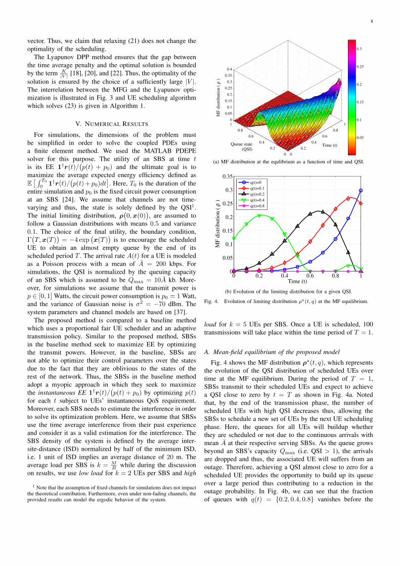
Fig. 4. Evolution of limiting distribution ρ?(t, q) at the MF equilibrium.

load for k = 5 UEs per SBS. Once a UE is scheduled, 100transmissions will take place within the time period of T = 1.

A. Mean-field equilibrium of the proposed model

Fig. 4 shows the MF distribution ρ?(t, q), which representsthe evolution of the QSI distribution of scheduled UEs overtime at the MF equilibrium. During the period of T = 1,SBSs transmit to their scheduled UEs and expect to achievea QSI close to zero by t = T as shown in Fig. 4a. Notedthat, by the end of the transmission phase, the number ofscheduled UEs with high QSI decreases thus, allowing theSBSs to schedule a new set of UEs by the next UE schedulingphase. Here, the queues for all UEs will buildup whetherthey are scheduled or not due to the continuous arrivals withmean A at their respective serving SBSs. As the queue growsbeyond an SBS’s capacity Qmax (i.e. QSI > 1), the arrivalsare dropped and thus, the associated UE will suffers from anoutage. Therefore, achieving a QSI almost close to zero for ascheduled UE provides the opportunity to build up its queueover a large period thus contributing to a reduction in theoutage probability. In Fig. 4b, we can see that the fractionof queues with q(t) = {0.2, 0.4, 0.8} vanishes before the

9

0

0.2

0.4

0.6

0.8

1

0

0.2

0.4

0.6

0.8

10.2

0.4

0.6

0.8

1

Time (t)Queue state

(QSI)

Eq

uil

ibri

um

tra

nsm

it p

ow

er [

W]

0.4

0.5

0.6

0.7

0.8

0.9

1

(a) Transmit power at the MF equilibrium as a function of time andQSI.

0 0.2 0.4 0.6 0.8 1

0.4

0.5

0.6

0.7

0.8

0.9

1

Time (t)

Eq

uil

ibri

um

tra

nsm

it p

ow

er [

W]

q(t)=0

q(t)=0.2

q(t)=0.4

q(t)=0.6

q(t)=0.8

q(t)=1

(b) Evolution of the transmit power for a given QSI.

Fig. 5. Evolution of transmit power p?(t, q) at the MF equilibrium.

transmission duration ends. As time evolves, the queues getempty based on the rates prior to new arrivals and thus, anoscillation is observed for the queue fractions with q(t) = 0.4while q(t) = 0 exhibits a monotonic increase.

The transmit power policy at the MF equilibrium is shownin Fig. 5. It can be observed that a higher transmit power isneeded when the QSI is high and this power can be reduced atlow QSI, showing the overall EE of the proposed approach. Att = 0, a moderate transmit power is used even for UEs withhigh QSI. Thus, SBSs prevent unnecessary interference withinthe system. As the scheduling period arrives to an end, werecall that the choice of Γ

(T,x(T )

)= −4 exp

(x(T )

)forces

SBSs to obtain smaller QSI at t = T . For UEs with low QSI,SBSs use moderate transmit power to maximize EE. However,for UEs with high QSI, SBSs use higher transmit power toprovide high data rates in order to empty their respectivequeues as well as preventing outages. Thus, as time evolves,SBSs increase their transmit power for UEs with high QSI asillustrated in Fig. 5b thereby improving the final utility.

B. Energy efficiency and outage comparisonsIn Fig. 6a, we show the EE of the system in terms of the

number of bits transmitted per joule of energy consumed as

3.5 4 4.5 5 5.5 6 6.50

2

4

6

8

10

Inter site distance

Aver

age

ener

gy

eff

icie

ncy

[b

its/

J/H

z]

ultra dense sparse

Baseline model: k=5

Baseline model: k=2

Proposed model: k=5

Proposed model: k=2

low load

high load

(a) Comparison of EE in terms of transmit bits per unit energy for lowand high loads k = {2, 5}.

3.5 4 4.5 5 5.5 6 6.510

−5

10−4

10−3

10−2

10−1

100

Inter site distance

Outa

ge

pro

bab

ilit

y

ultra dense sparse

Baseline model: k=5

Baseline model: k=2

Proposed model: k=5

Proposed model: k=2

low load

high load

(b) Comparison of outage probabilities for low and high loads k ={2, 5}.

Fig. 6. Comparison of the behavior of EE and outage probabilities fordifferent SBS densities.

a function of ISD. Here, the load represents the number ofUEs served by an SBS. For a dense network (ISD = 3.5), theproposed method will improve EE of about 5% compared tothe baseline model with k = 2. However, as the load increasesto k = 5, this EE improvement will reach up to 48.8%. Theseimproved EE for the dense scenario shown in the proposedapproach is due to its ability to adapt to the dynamics ofthe network, as enabled by the stochastic game formulationand its MF approximation. Naturally, as the network becomesless dense, the advantages of the proposed approach willbe smaller. For instance, for a non-dense network with anISD = 6.5 and k = 5 UEs per SBS, performance advantagesof the MF approach decreases to 4.8% as shown in Fig. 6a. Fora very lightly loaded and non-dense network, such as whenISD = 6.5 and k = 2 UEs per SBS, the use of the baselinemethod will be slightly more advantageous when compared tothe proposed approach. This advantage is of about 14.1% ofimprovement in the EE.

Fig. 6b illustrates the outage probability as a function ofISD. Here, the outage probability is defined as the fraction ofunsatisfied UEs whose arrivals are dropped due to limitationsof the queue capacity. It can be noted that the proposed

10

2 3 4 5 60

1

2

3

4

5

6

7

8

Load per BS

Av

erag

e en

ergy

eff

icie

ncy

[b

its/

J/H

z]

high loadlow load

Baseline model: ISD=3.5

Baseline model: ISD=5.75

Proposed model: ISD=3.5

Proposed model: ISD=5.75

ultra−dense

sparse

(a) Comparison of EE for sparse and dense networks ISD = {5.75, 3.5}.

2 3 4 5 610

−6

10−5

10−4

10−3

10−2

10−1

100

Load per BS

Ou

tage

pro

bab

ilit

y

high loadlow load

Baseline model: ISD=3.5

Baseline model: ISD=5.75

Proposed model: ISD=3.5

Proposed model: ISD=5.75

ultra dense

sparse

(b) Comparison of outage probability for sparse and dense networksISD = {5.75, 3.5}.

Fig. 7. Comparison of the behavior of EE and outage probabilities fordifferent loads.

method uses smart UE scheduling and transmit power policybased on QSI which ensures a higher UE QoS. Although thebaseline model optimizes the transmit power with the goalof improving EE, it is unable to track the QSI dynamics andadapt the UE scheduling accordingly. Thus, higher numberof UEs suffer from outages. As the network becomes highlyloaded and more dense (i.e., as the number of SBSs and UEsincrease), the number of UEs in outage will naturally increasefor both approaches. This is due to the increased interferenceand the high average waiting time due to increased numberof UEs. From Fig. 6b, we observe that the proposed methodyields 91.8% and 41.8% reductions in outages compared to thebaseline model for both low and high loads, respectively, inUDNs. For a sparse network, the outage reductions are 92.2%and 99.5% for low and high loads, respectively.

Fig. 7a shows how EE varies with the number of UEs perSBS (i.e., load). We can observe that the proposed methodshows higher EE gains for dense networks. For k = 6 UEsper SBS and ISD = 3.5, the proposed method yields an EEgain of 70.7% compared to the baseline model while reaching20.3% as the network becomes sparse with ISD = 5.75. Thegains in the proposed method for dense scenarios are due

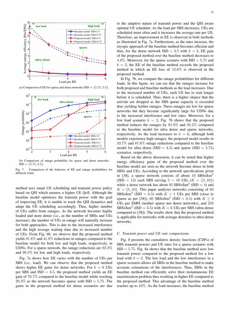
to the adaptive nature of transmit power and the QSI awareoptimal UE scheduler. As the load per SBS decreases, UEs arescheduled more often and it increases the average rate per UE.Therefore, an improvement in EE is observed in both methodsas illustrated in Fig. 7a. Furthermore, as the rates increase, themyopic approach of the baseline method becomes efficient andthus, for the dense network ISD = 3.5 with k = 2, EE gainof the proposed method over the baseline method decreases to4.8%. Moreover, for the sparse scenario with ISD = 5.75 andk = 2, the EE of the baseline method exceeds the proposedmethod in which an EE loss of 12.6% is observed in theproposed method.

In Fig. 7b, we compare the outage probabilities for differentloads. In this figure, we can see that the outages increase forboth proposed and baseline methods as the load increases. Dueto the increased number of UEs, each UE has to wait longerbefore it is scheduled. Thus, there is a higher chance that thearrivals are dropped as the SBS queue capacity is exceededthus yielding further outages. These outages are low for sparsenetworks but they become significantly large for UDNs dueto the increased interference and low rates. Moreover, for alow load scenario k = 2, Fig. 7b shows that the proposedmethod reduces the outages by 91.8% and 92.2% comparedto the baseline model for ultra dense and sparse networks,respectively. As the load increases to k = 6, although bothmodels experience high outages, the proposed model results in33.7% and 87.6% outage reductions compared to the baselinemodel for ultra dense (ISD = 3.5) and sparse (ISD = 5.75)scenarios, respectively.

Based on the above discussion, it can be noted that higherenergy efficiency gains of the proposed method over thebaseline model are seen as the network become dense in bothSBSs and UEs. According to the network specifications givenin [38], a sparse network consists of about 10 SBSs/km2

(ISD = 12) each SBS serving 5 ∼ 10 UEs (K = {5, 10})while a dense network has about 95 SBSs/km2 (ISD = 4) andK = {5, 10}. This paper analyzes networks consisting of 60SBSs/km2 (ISD = 6.5) with K = 1 UEs per SBS (close tosparse as per [38]), 60 SBSs/km2 (ISD = 6.5) with K ≥ 3UEs per SSBS (neither sparse nor dense networks), and 250SBSs/km2 (ISD = 3.5) with K = 6 UEs per SBS (ultra-densecompared to [38]). The results show that the proposed methodis applicable for networks with average densities to ultra-densenetworks.

C. Transmit power and UE rate comparisons

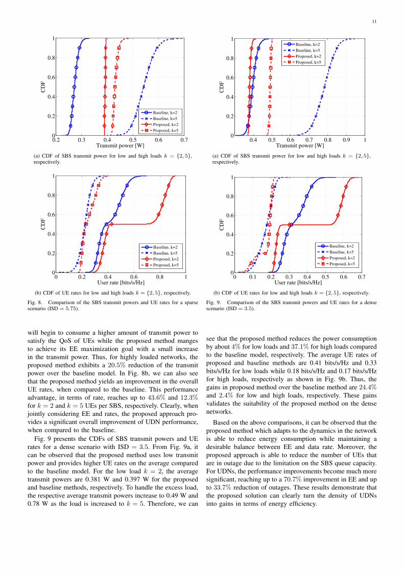
Fig. 8 presents the cumulative density functions (CDFs) ofSBS transmit powers and UE rates for a sparse scenario withISD = 5.75. Fig. 8a shows that the baseline method uses lowtransmit power compared to the proposed method for a lowload with k = 2. The low load and the low interference in asparse scenario allows all SBSs in the baseline method to makeaccurate estimations of the interferences. Thus, SBSs in thebaseline method can efficiently solve their instantaneous EEmaximization problem thus resulting in higher EE compared tothe proposed method. This advantage of the baseline methodreaches up to 43%. As the load increases, the baseline method

11

0.2 0.3 0.4 0.5 0.6 0.70

0.2

0.4

0.6

0.8

1

Transmit power [W]

CD

F

Baseline, k=2

Baseline, k=5

Proposed, k=2

Proposed, k=5

(a) CDF of SBS transmit power for low and high loads k = {2, 5},respectively.

0 0.2 0.4 0.6 0.8 10

0.2

0.4

0.6

0.8

1

User rate [bits/s/Hz]

CD

F

Baseline, k=2

Baseline, k=5

Proposed, k=2

Proposed, k=5

(b) CDF of UE rates for low and high loads k = {2, 5}, respectively.

Fig. 8. Comparison of the SBS transmit powers and UE rates for a sparsescenario (ISD = 5.75).

will begin to consume a higher amount of transmit power tosatisfy the QoS of UEs while the proposed method mangesto achieve its EE maximization goal with a small increasein the transmit power. Thus, for highly loaded networks, theproposed method exhibits a 20.5% reduction of the transmitpower over the baseline model. In Fig. 8b, we can also seethat the proposed method yields an improvement in the overallUE rates, when compared to the baseline. This performanceadvantage, in terms of rate, reaches up to 43.6% and 12.3%for k = 2 and k = 5 UEs per SBS, respectively. Clearly, whenjointly considering EE and rates, the proposed approach pro-vides a significant overall improvement of UDN performance,when compared to the baseline.

Fig. 9 presents the CDFs of SBS transmit powers and UErates for a dense scenario with ISD = 3.5. From Fig. 9a, itcan be observed that the proposed method uses low transmitpower and provides higher UE rates on the average comparedto the baseline model. For the low load k = 2, the averagetransmit powers are 0.381 W and 0.397 W for the proposedand baseline methods, respectively. To handle the excess load,the respective average transmit powers increase to 0.49 W and0.78 W as the load is increased to k = 5. Therefore, we can

0.4 0.5 0.6 0.7 0.8 0.9 10

0.2

0.4

0.6

0.8

1

Transmit power [W]

CD

F

Baseline, k=2

Baseline, k=5

Proposed, k=2

Proposed, k=5

(a) CDF of SBS transmit power for low and high loads k = {2, 5},respectively.

0 0.1 0.2 0.3 0.4 0.5 0.6 0.70

0.2

0.4

0.6

0.8

1

User rate [bits/s/Hz]

CD

F

Baseline, k=2

Baseline, k=5

Proposed, k=2

Proposed, k=5

(b) CDF of UE rates for low and high loads k = {2, 5}, respectively.

Fig. 9. Comparison of the SBS transmit powers and UE rates for a densescenario (ISD = 3.5).

see that the proposed method reduces the power consumptionby about 4% for low loads and 37.1% for high loads comparedto the baseline model, respectively. The average UE rates ofproposed and baseline methods are 0.41 bits/s/Hz and 0.33bits/s/Hz for low loads while 0.18 bits/s/Hz and 0.17 bits/s/Hzfor high loads, respectively as shown in Fig. 9b. Thus, thegains in proposed method over the baseline method are 24.4%and 2.4% for low and high loads, respectively. These gainsvalidates the suitability of the proposed method on the densenetworks.

Based on the above comparisons, it can be observed that theproposed method which adapts to the dynamics in the networkis able to reduce energy consumption while maintaining adesirable balance between EE and data rate. Moreover, theproposed approach is able to reduce the number of UEs thatare in outage due to the limitation on the SBS queue capacity.For UDNs, the performance improvements become much moresignificant, reaching up to a 70.7% improvement in EE and upto 33.7% reduction of outages. These results demonstrate thatthe proposed solution can clearly turn the density of UDNsinto gains in terms of energy efficiency.

12

0 0.2 0.4 0.6 0.8 1−11

−10

−9

−8

−7

−6

−5

−4

−3

Final queue state Q(T)

Uti

lity

bo

un

dar

y c

on

dit

ion

Exponential bound

Uniform bound

Linear bound

Fig. 10. Different boundary conditions used for the utility at the end ofscheduling period.

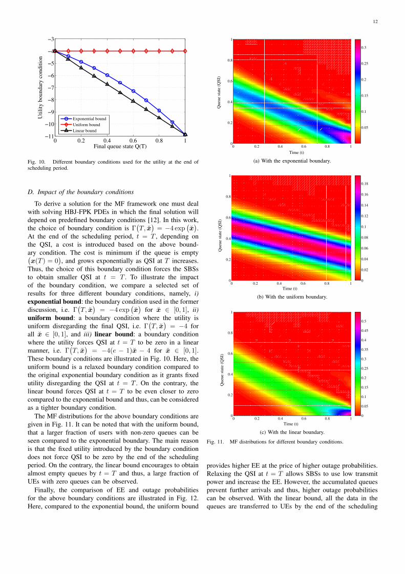
D. Impact of the boundary conditions

To derive a solution for the MF framework one must dealwith solving HBJ-FPK PDEs in which the final solution willdepend on predefined boundary conditions [12]. In this work,the choice of boundary condition is Γ

(T, x

)= −4 exp

(x).

At the end of the scheduling period, t = T , depending onthe QSI, a cost is introduced based on the above bound-ary condition. The cost is minimum if the queue is empty(x(T ) = 0

), and grows exponentially as QSI at T increases.

Thus, the choice of this boundary condition forces the SBSsto obtain smaller QSI at t = T . To illustrate the impactof the boundary condition, we compare a selected set ofresults for three different boundary conditions, namely, i)exponential bound: the boundary condition used in the formerdiscussion, i.e. Γ

(T, x

)= −4 exp

(x)

for x ∈ [0, 1], ii)uniform bound: a boundary condition where the utility isuniform disregarding the final QSI, i.e. Γ

(T, x

)= −4 for

all x ∈ [0, 1], and iii) linear bound: a boundary conditionwhere the utility forces QSI at t = T to be zero in a linearmanner, i.e. Γ

(T, x

)= −4(e − 1)x − 4 for x ∈ [0, 1].

These boundary conditions are illustrated in Fig. 10. Here, theuniform bound is a relaxed boundary condition compared tothe original exponential boundary condition as it grants fixedutility disregarding the QSI at t = T . On the contrary, thelinear bound forces QSI at t = T to be even closer to zerocompared to the exponential bound and thus, can be consideredas a tighter boundary condition.

The MF distributions for the above boundary conditions aregiven in Fig. 11. It can be noted that with the uniform bound,that a larger fraction of users with non-zero queues can beseen compared to the exponential boundary. The main reasonis that the fixed utility introduced by the boundary conditiondoes not force QSI to be zero by the end of the schedulingperiod. On the contrary, the linear bound encourages to obtainalmost empty queues by t = T and thus, a large fraction ofUEs with zero queues can be observed.

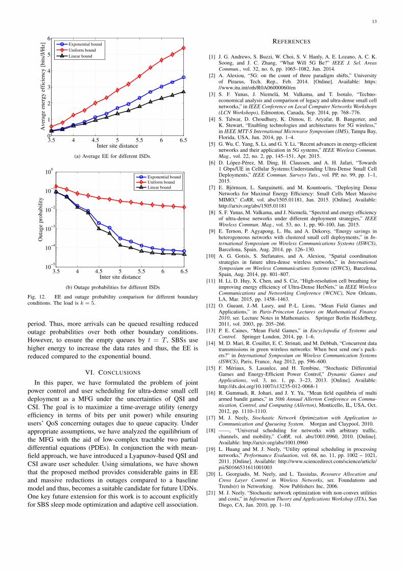
Finally, the comparison of EE and outage probabilitiesfor the above boundary conditions are illustrated in Fig. 12.Here, compared to the exponential bound, the uniform bound

0 0.2 0.4 0.6 0.8 10

0.2

0.4

0.6

0.8

1

Time (t)

Queue s

tate

(Q

SI)

0.05

0.1

0.15

0.2

0.25

0.3

(a) With the exponential boundary.

0 0.2 0.4 0.6 0.8 10

0.2

0.4

0.6

0.8

1

Time (t)

Queue s

tate

(Q

SI)

0

0.02

0.04

0.06

0.08

0.1

0.12

0.14

0.16

0.18

(b) With the uniform boundary.

0 0.2 0.4 0.6 0.8 10

0.2

0.4

0.6

0.8

1

Time (t)

Queue s

tate

(Q

SI)

0

0.05

0.1

0.15

0.2

0.25

0.3

0.35

0.4

0.45

0.5

(c) With the linear boundary.

Fig. 11. MF distributions for different boundary conditions.

provides higher EE at the price of higher outage probabilities.Relaxing the QSI at t = T allows SBSs to use low transmitpower and increase the EE. However, the accumulated queuesprevent further arrivals and thus, higher outage probabilitiescan be observed. With the linear bound, all the data in thequeues are transferred to UEs by the end of the scheduling

13

3.5 4 4.5 5 5.5 6 6.50

1

2

3

4

5

6

Inter site distance

Av

erag

e en

ergy

eff

icie

ncy

[b

its/

J/H

z]

Exponential bound

Uniform bound

Linear bound

(a) Average EE for different ISDs.

3.5 4 4.5 5 5.5 6 6.510

−5

10−4

10−3

10−2

10−1

100

Inter site distance

Outa

ge

pro

bab

ilit

y

Exponential bound

Uniform bound

Linear bound

(b) Outage probabilities for different ISDs

Fig. 12. EE and outage probability comparison for different boundaryconditions. The load is k = 5.

period. Thus, more arrivals can be queued resulting reducedoutage probabilities over both other boundary conditions.However, to ensure the empty queues by t = T , SBSs usehigher energy to increase the data rates and thus, the EE isreduced compared to the exponential bound.

VI. CONCLUSIONS

In this paper, we have formulated the problem of jointpower control and user scheduling for ultra-dense small celldeployment as a MFG under the uncertainties of QSI andCSI. The goal is to maximize a time-average utility (energyefficiency in terms of bits per unit power) while ensuringusers’ QoS concerning outages due to queue capacity. Underappropriate assumptions, we have analyzed the equilibrium ofthe MFG with the aid of low-complex tractable two partialdifferential equations (PDEs). In conjunction the with mean-field approach, we have introduced a Lyapunov-based QSI andCSI aware user scheduler. Using simulations, we have shownthat the proposed method provides considerable gains in EEand massive reductions in outages compared to a baselinemodel and thus, becomes a suitable candidate for future UDNs.One key future extension for this work is to account explicitlyfor SBS sleep mode optimization and adaptive cell association.

REFERENCES

[1] J. G. Andrews, S. Buzzi, W. Choi, S. V. Hanly, A. E. Lozano, A. C. K.Soong, and J. C. Zhang, “What Will 5G Be?” IEEE J. Sel. AreasCommun., vol. 32, no. 6, pp. 1065–1082, Jun. 2014.

[2] A. Alexiou, “5G: on the count of three paradigm shifts,” Universityof Piraeus, Tech. Rep., Feb. 2014. [Online]. Available: https://www.itu.int/oth/R0A06000060/en

[3] S. F. Yunas, J. Niemela, M. Valkama, and T. Isotalo, “Techno-economical analysis and comparison of legacy and ultra-dense small cellnetworks,” in IEEE Conference on Local Computer Networks Workshops(LCN Workshops), Edmonton, Canada, Sep. 2014, pp. 768–776.

[4] S. Talwar, D. Choudhury, K. Dimou, E. Aryafar, B. Bangerter, andK. Stewart, “Enabling technologies and architectures for 5G wireless,”in IEEE MTT-S International Microwave Symposium (IMS), Tampa Bay,Florida, USA, Jun. 2014, pp. 1–4.

[5] G. Wu, C. Yang, S. Li, and G. Y. Li, “Recent advances in energy-efficientnetworks and their application in 5G systems,” IEEE Wireless Commun.Mag., vol. 22, no. 2, pp. 145–151, Apr. 2015.

[6] D. Lopez-Perez, M. Ding, H. Claussen, and A. H. Jafari, “Towards1 Gbps/UE in Cellular Systems:Understanding Ultra-Dense Small CellDeployments,” IEEE Commun. Surveys Tuts., vol. PP, no. 99, pp. 1–1,2015.

[7] E. Bjornson, L. Sanguinetti, and M. Kountouris, “Deploying DenseNetworks for Maximal Energy Efficiency: Small Cells Meet MassiveMIMO,” CoRR, vol. abs/1505.01181, Jun. 2015. [Online]. Available:http://arxiv.org/abs/1505.01181

[8] S. F. Yunas, M. Valkama, and J. Niemela, “Spectral and energy efficiencyof ultra-dense networks under different deployment strategies,” IEEEWireless Commun. Mag., vol. 53, no. 1, pp. 90–100, Jan. 2015.

[9] E. Ternon, P. Agyapong, L. Hu, and A. Dekorsy, “Energy savings inheterogeneous networks with clustered small cell deployments,” in In-ternational Symposium on Wireless Communications Systems (ISWCS),Barcelona, Spain, Aug. 2014, pp. 126–130.

[10] A. G. Gotsis, S. Stefanatos, and A. Alexiou, “Spatial coordinationstrategies in future ultra-dense wireless networks,” in InternationalSymposium on Wireless Communications Systems (ISWCS), Barcelona,Spain, Aug. 2014, pp. 801–807.

[11] H. Li, D. Huy, X. Chen, and S. Ciz, “High-resolution cell breathing forimproving energy efficiency of Ultra-Dense HetNets,” in IEEE WirelessCommunications and Networking Conference (WCNC), New Orleans,LA, Mar. 2015, pp. 1458–1463.

[12] O. Gueant, J.-M. Lasry, and P.-L. Lions, “Mean Field Games andApplications,” in Paris-Princeton Lectures on Mathematical Finance2010, ser. Lecture Notes in Mathematics. Springer Berlin Heidelberg,2011, vol. 2003, pp. 205–266.

[13] P. E. Caines, “Mean Field Games,” in Encyclopedia of Systems andControl. Springer London, 2014, pp. 1–6.

[14] M. D. Mari, R. Couillet, E. C. Strinati, and M. Debbah, “Concurrent datatransmissions in green wireless networks: When best send one’s pack-ets?” in International Symposium on Wireless Communication Systems(ISWCS), Paris, France, Aug 2012, pp. 596–600.

[15] F. Meriaux, S. Lasaulce, and H. Tembine, “Stochastic DifferentialGames and Energy-Efficient Power Control,” Dynamic Games andApplications, vol. 3, no. 1, pp. 3–23, 2013. [Online]. Available:http://dx.doi.org/10.1007/s13235-012-0068-1

[16] R. Gummadi, R. Johari, and J. Y. Yu, “Mean field equilibria of multiarmed bandit games,” in 50th Annual Allerton Conference on Commu-nication, Control, and Computing (Allerton), Monticello, IL, USA, Oct.2012, pp. 1110–1110.

[17] M. J. Neely, Stochastic Network Optimization with Application toCommunication and Queueing System. Morgan and Claypool, 2010.

[18] ——, “Universal scheduling for networks with arbitrary traffic,channels, and mobility,” CoRR, vol. abs/1001.0960, 2010. [Online].Available: http://arxiv.org/abs/1001.0960

[19] L. Huang and M. J. Neely, “Utility optimal scheduling in processingnetworks,” Performance Evaluation, vol. 68, no. 11, pp. 1002 – 1021,2011. [Online]. Available: http://www.sciencedirect.com/science/article/pii/S0166531611001003

[20] L. Georgiadis, M. Neely, and L. Tassiulas, Resource Allocation andCross Layer Control in Wireless Networks, ser. Foundations andTrends(r) in Networking. Now Publishers Inc, 2006.

[21] M. J. Neely, “Stochastic network optimization with non-convex utilitiesand costs,” in Information Theory and Applications Workshop (ITA), SanDiego, CA, Jan. 2010, pp. 1–10.

14

[22] D. Bethanabhotla, G. Caire, and M. J. Neely, “Adaptive video streamingfor wireless networks with multiple users and helpers,” IEEE Trans.Commun., vol. 63, pp. 268–285, Jan. 2015.

[23] T. S. Rappaport, Wireless Communications: Principles and Practice,2nd ed. Prentice Hall, 2002.

[24] C. Shuguang, A. J. Goldsmith, and A. Bahai, “Energy-constrainedmodulation optimization,” IEEE Trans. Wireless Commun., vol. 4, no. 5,pp. 2349–2360, Sep 2005.

[25] L. C. Evans, Partial Differential Equations, ser. Graduate Studies inMathematics. American Mathematical Society, 2010.

[26] O. R. B. de Oliveira, “The Implicit and the Inverse Function theorems:easy proofs,” CoRR, vol. abs/1212.2066, 2012. [Online]. Available:http://arxiv.org/abs/1212.2066

[27] R. Couillet and M. Debbah, Random Matrix Methods for WirelessCommunications. Cambridge University Press, 2011.

[28] R. Hekmat, Ad-hoc Networks: Fundamental Properties and NetworkTopologies. Springer Science & Business Media, Sep. 2006.

[29] R. Hekmat and X. An, “Relation between interference and neighbor at-tachment policies in ad-hoc and sensor networks,” International Journalof Hybrid Information Technology, vol. 1, no. 2, Apr. 2008.

[30] M. Haenggi and R. K. Ganti, “Interference in Large Wireless Networks,”Foundations and Trends R© in Networking, vol. 3, no. 2, pp. 127–248,Nov. 2009.

[31] G. Koch and F. Spizzichino, Exchangeability in Probability and Statis-tics: International Conference Proceedings. Elsevier Science Ltd, 1982.

[32] P. Gagliardini and C. Gourieroux, Granularity Theory with Applicationsto Finance and Insurance. Elsevier Science Ltd, 2014.

[33] H. Tembine and M. Huang, “Mean field difference games: McKean-Vlasov dynamics,” in IEEE Conference on Decision and Control andEuropean Control Conference (CDC-ECC), Orlando, Florida, USA, Dec.2011, pp. 1006–1011.

[34] R. Kwan, C. Leung, and J. Zhang, “Proportional Fair Multiuser Schedul-ing in LTE,” IEEE Signal Process. Lett., vol. 16, no. 6, pp. 461–464,Jun. 2009.

[35] R. Fritzsche, P. Rost, and G. P. Fettweis, “Robust Rate Adaptation andProportional Fair Scheduling with Imperfect CSI,” IEEE Trans. WirelessCommun., vol. PP, no. 99, pp. 1–1, 2015.

[36] S. Boyd and L. Vandenberghe, Convex Optimization. CambridgeUniversity Press, 2004.

[37] 3GPP, “Evolved universal terrestrial radio access (E-UTRA); Furtheradvancements for E-UTRA physical layer aspects,” 3rd Generation Part-nership Project (3GPP), TR 36.814-900, Mar. 2010. [Online]. Available:http://www.3gpp.org/ftp/Specs/archive/36 series/36.814/36814-900.zip

[38] ——, “Small cell enhancements for E-UTRA and E-UTRAN - Physicallayer aspects,” 3rd Generation Partnership Project (3GPP), TR 36.872,Dec. 2013. [Online]. Available: http://www.3gpp.org/ftp/Specs/archive/36 series/36.872/36872-c10.zip

Sumudu Samarakoon received his B. Sc. (Hons.)degree in Electronic and Telecommunication En-gineering from the University of Moratuwa, SriLanka and the M. Eng. degree from the AsianInstitute of Technology, Thailand in 2009 and 2011,respectively. He is currently pursuing hid Dr. Techdegree in Communications Engineering at the Uni-versity of Oulu, Finland. Sumudu is also a memberof the research staff of the Centre for WirelessCommunications (CWC), Oulu, Finland. His mainresearch interests are in heterogeneous networks,

radio resource management, machine learning, and game theory.

Mehdi Bennis received his M.Sc. degree in Electri-cal Engineering jointly from the EPFL, Switzerlandand the Eurecom Institute, France in 2002. From2002 to 2004, he worked as a research engineer atIMRA-EUROPE investigating adaptive equalizationalgorithms for mobile digital TV. In 2004, he joinedthe Centre for Wireless Communications (CWC)at the University of Oulu, Finland as a researchscientist. In 2008, he was a visiting researcher at theAlcatel-Lucent chair on flexible radio, SUPELEC.He obtained his Ph.D. in December 2009 on spec-

trum sharing for future mobile cellular systems.His main research interests are in radio resource management, heteroge-

neous networks, game theory and machine learning in 5G networks andbeyond. He has co-authored one book and published more than 100 researchpapers in international conferences, journals and book chapters. He wasthe recipient of the prestigious 2015 Fred W. Ellersick Prize from theIEEE Communications Society. Dr. Bennis serves as an editor for the IEEETransactions on Wireless Communications.

Walid Saad (S’07, M’10, SM15) Walid Saad re-ceived his Ph.D degree from the University of Osloin 2010. Currently, he is an Assistant Professor andthe Steven O. Lane Junior Faculty Fellow at theDepartment of Electrical and Computer Engineer-ing at Virginia Tech, where he leads the NetworkScience, Wireless, and Security (NetSciWiS) labo-ratory, within the Wireless@VT research group. Hisresearch interests include wireless networks, gametheory, cybersecurity, and cyber-physical systems.Dr. Saad is the recipient of the NSF CAREER award

in 2013, the AFOSR summer faculty fellowship in 2014, and the YoungInvestigator Award from the Office of Naval Research (ONR) in 2015. Hewas the author/co-author of five conference best paper awards at WiOpt in2009, ICIMP in 2010, IEEE WCNC in 2012, IEEE PIMRC in 2015, and IEEESmartGridComm in 2015. He is the recipient of the 2015 Fred W. EllersickPrize from the IEEE Communications Society. Dr. Saad serves as an editorfor the IEEE Transactions on Wireless Communications, IEEE Transactionson Communications, and IEEE Transactions on Information Forensics andSecurity.

Merouane Debbah (S’01-AM’03-M’04-SM’08-1030 F’15) entered the Ecole Normale Superieurede Cachan (France) in 1996 where he received hisM.Sc and Ph.D. degrees respectively. He worked forMotorola Labs (Saclay, France) from 1999-2002 andthe Vienna Research Center for Telecommunications(Vienna, Austria) until 2003. From 2003 to 2007, hejoined the Mobile Communications department ofthe Institut Eurecom (Sophia Antipolis, France) asan Assistant Professor. Since 2007, he is a Full Pro-fessor at CentraleSupelec (Gif-sur-Yvette, France).

From 2007 to 2014, he was the director of the Alcatel-Lucent Chair onFlexible Radio. Since 2014, he is Vice-President of the Huawei FranceR&D center and director of the Mathematical and Algorithmic Sciences Lab.His research interests lie in fundamental mathematics, algorithms, statistics,information & communication sciences research. He is an Associate Editorin Chief of the journal Random Matrix: Theory and Applications and was anassociate and senior area editor for IEEE Transactions on Signal Processingrespectively in 2011-2013 and 2013-2014. Merouane Debbah is a recipient ofthe ERC grant MORE (Advanced Mathematical Tools for Complex NetworkEngineering). He is a IEEE Fellow, a WWRF Fellow and a member of theacademic senate of Paris-Saclay. He has managed 8 EU projects and morethan 24 national and international projects. He received 14 best paper awards,among which the 2007 IEEE GLOBECOM best paper award, the Wi-Opt2009 best paper award, the 2010 Newcom++ best paper award, the WUNCogCom Best Paper 2012 and 2013 Award, the 2014 WCNC best paperaward, the 2015 ICC best paper award, the 2015 IEEE CommunicationsSociety Leonard G. Abraham Prize and 2015 IEEE Communications SocietyFred W. Ellersick Prize as well as the Valuetools 2007, Valuetools 2008,CrownCom2009, Valuetools 2012 and SAM 2014 best student paper awards.He is the recipient of the Mario Boella award in 2005, the IEEE GlavieuxPrize Award in 2011 and the Qualcomm Innovation Prize Award in 2012.

15

Matti Latva-aho received the M.Sc., Lic.Tech. andDr. Tech (Hons.) degrees in Electrical Engineeringfrom the University of Oulu, Finland in 1992, 1996and 1998, respectively. From 1992 to 1993, hewas a Research Engineer at Nokia Mobile Phones,Oulu, Finland after which he joined Centre forWireless Communications (CWC) at the Universityof Oulu. Prof. Latva-aho was Director of CWCduring the years 1998-2006 and Head of Departmentfor Communication Engineering until August 2014.Currently he is Professor of Digital Transmission

Techniques at the University of Oulu. His research interests are related tomobile broadband communication systems and currently his group focuseson 5G systems research. Prof. Latva-aho has published 300+ conference orjournal papers in the field of wireless communications.