uknowledge / university of kentucky libraries
TRANSCRIPT

University of Kentucky University of Kentucky
UKnowledge UKnowledge
University of Kentucky Master's Theses Graduate School
2011
INFLUENCE OF FAN OPERATION ON FAN ASSESSMENT INFLUENCE OF FAN OPERATION ON FAN ASSESSMENT
NUMERATION SYSTEM (FANS) TEST RESULTS NUMERATION SYSTEM (FANS) TEST RESULTS
Gabriela Munhoz Morello University of Kentucky, [email protected]
Right click to open a feedback form in a new tab to let us know how this document benefits you. Right click to open a feedback form in a new tab to let us know how this document benefits you.
Recommended Citation Recommended Citation Morello, Gabriela Munhoz, "INFLUENCE OF FAN OPERATION ON FAN ASSESSMENT NUMERATION SYSTEM (FANS) TEST RESULTS" (2011). University of Kentucky Master's Theses. 153. https://uknowledge.uky.edu/gradschool_theses/153
This Thesis is brought to you for free and open access by the Graduate School at UKnowledge. It has been accepted for inclusion in University of Kentucky Master's Theses by an authorized administrator of UKnowledge. For more information, please contact [email protected].

ABSTRACT OF THESIS
INFLUENCE OF FAN OPERATION ON FAN ASSESSMENT NUMERATION SYSTEM (FANS) TEST RESULTS
The use of velocity traverses to measure in-situ air flow rate of ventilation fans can be subject to significant errors. The Fan Assessment Numeration System (FANS)
was developed by the USD-ARS Southern Poultry Research Laboratory and refined at the University of Kentucky to measure air flow of fans in-situ. The procedures for using
the FANS unit to test fans in-situ are not completely standardized. This study evaluated the effect of operating fan positions relative to the FANS unit for ten 1.22 m diameter fans in two types of poultry barns, with fans placed immediately next to each other and
1.6 m apart. Fans were tested with the FANS unit placed near both the intake and discharge sides of the tested fans. Data were analyzed as two Generalized Randomized
Complete Block designs (GRCB), with a 2 (FANS inside or outside) x 6 (operating fan combinations) factorial arrangement of treatments. Results showed significant differences as much as 12.6 ± 4.4% between air flow values obtained under conditions of different
operating fan combinations. Placing the FANS unit outside provided valid fan test results. A standardized procedure for using the FANS unit to test fans in-situ was elaborated and
presented in this work.
KEYWORDS: Fan Assessment Numeration System (FANS), Fan Performance,
Ventilation Rate, In-Situ Fan Performance, Poultry Houses.
Gabriela Munhoz Morello
06/15/2011
INFLUENCE OF FAN OPERATION ON FAN ASSESSMENT NUMERATION SYSTEM (FANS) TEST RESULTS.
By
Gabriela Munhoz Morello
Dr. Douglas G. Overhults
Director of Thesis
Dr. Dwayne Edwards
Director of Graduate Studies
06/15/2011

RULES FOR THE USE OF DISSERTATIONS
Unpublished dissertations submitted for the Master’s degree and deposited in the
University of Kentucky Library are as a rule open for inspection, but are to be used only with due regard to the rights of the authors. Bibliographical references may be noted, but quotations or summaries of parts may be published only with permission of the author,
and with the usual scholarly acknowledgements.
Extensive copying or publication of the thesis in whole or in part also requires the consent of the Dean of the Graduate School of the University of Kentucky.
A library that borrows this dissertation for use by its patrons is expected to secure the signature of each user.
Name Date

THESIS
Gabriela Munhoz Morello
The Graduate School
University of Kentucky
2011

INFLUENCE OF FAN OPERATION ON FAN ASSESSMENT NUMERATION SYSTEM (FANS) TEST RESULTS
THESIS
A thesis submitted in partial fulfillment of the
requirements for the degree of Master of Science in Biosystems and Agricultural Engineering
At the University of Kentucky
By
Gabriela Munhoz Morello
Lexington, Kentucky
Director: Dr. Douglas G. Overhults, Associate Extension Professor Biosystems and
Agricultural Engineering
Lexington, Kentucky
2011
Copyright © Gabriela Munhoz Morello 2011

To those who inspire and guide me
on accomplishing my dreams.

Àqueles que me inspiram e conduzem
a realizar meus sonhos.

iii
ACKNOWLEDGMENTS
Many people contributed either directly or indirectly to the elaboration of the
following thesis and I feel honored to have enjoyed and benefited from their insights and
companions. First, I wish to thank my thesis Chair, Dr. Douglas Overhults, for his
guidance during the Masters program. Dr. Overhults contributed with innumerous
instructive comments, which allowed me to accomplish this high quality work. Dr.
Overhults together with his wife, Elaine, ensured that all the necessary support was
provided for my living and work environments, for which I am really thankful. Their
presence and care made me feel at home.
Next, I wish to thank Dr. George Day for his excellent advices and thoughts,
which I will carry with me everywhere I go throughout my academic career and life. Dr.
Day and his family included me, along with the other members of our research group, as
parts of a larger beloved family. In addition, I would like to thank Dr. Richard Gates for
sharing his knowledge and work experience with me, which was essential to accomplish
this project. Dr. Daniella Moura was the first person to motivate me to pursue the
academic career and I am deeply grateful for all her motivation, help and friendship.
My appreciation goes to the Kentucky poultry producers (who remain anonymous
for confidentiality purposes), Mr. John Earnest Jr., Mr. Steven Ford, Ms. Christina
Lyvers, Ms. Karla Lima and Ms. Carla Soares, who contributed with the data collection
for the project, as well as the entire Biosystems and Agricultural Engineering community,
which welcomed me to University of Kentucky. Also, I would like to thank my
“Lexington familiy” Ms. Maira Pecegueiro do Amaral, Ms. Tatiana Gravena Ferreira,
Mr. Rodrigo Zandonadi, Dr. Enrique Alves, Dr. Guilherme Del Nero Maia and Mr. Joe

iv
Luck, who helped me either with my Masters program or with my personal life in
Lexington, KY. These people shared wonderful moments with me, which will eternally
remain in my mind and heart.
I would like to extend my appreciation to the friends that I made during my
Masters program, such as Mr. Lucas de Melo, Mr. Flávio Damasceno and our large
Brazilian community in the United States, who brought me joy everyday during my
Masters program. I wish to acknowledge all my friends from Brazil and family who
warmly welcomed me to Brazil whenever I could visit them, especially my uncle Mr.
Marcelo Morello, my grandparents Ms. Maria and Mr. João Bueno, my aunt and her
husband Ms. Keli and Mr. Gustavo Medeiros, my great-aunt and great-uncle Ms. Izete
and Mr. Edson de Ávila and their family, my sister Ms. Mirella Morello, my “step-
grandmother” Ms. Angelina Barrichelo, my “step-father” Mr. Paulo Victor Licre, my
friends Ms. Livia Gontijo, Ms. Sulimar Nogueira and my group of friends “the félas”.
I wish to acknowledge my mother Ms. Kátia Bueno for motivating me to pursue
graduate studies since I started my undergraduate studies and for being an example of
success in her professional life. In addition, I want to thank my father Mr. Marcos
Morello for the financial support to my studies, while I was in Brazil, and for the
moments of laughs that we shared during my visits to my home country. I appreciate Mr.
Luiz Carrijo for the help and care dedicated to my mother and her family during my
absence.
Special thanks go to my grandmother, Ms. Gleuza Munhoz Morello, who instilled
in me, from an early age, the desire and skills to obtain the Master’s in the Engineering
School, as well as to keep studying and learning throughout my life. Also, I wish to thank

v
my grandfather Mr. José Carlos Morello, for patiently waiting for me and picking me up
after every English class, during nine years of studying this language. The English classes
allowed me to write and communicate in English and made it possible to accomplish my
Masters degree at University of Kentucky as well as to write the following thesis in
English. I would like to acknowledge my boyfriend, Mr. Ígor Moreira Lopes, for the
love, complicity and for helping me with my research work, as well as his parents, Ms.
Glória and Mr. Geraldo Lopes, for the encouragement, advices and friendship.
Finally, I would like to thank the University of Kentucky, the College of
Agriculture and the College of Engineering for the opportunity. I wish to thank the
Kentucky Poultry Federation and the Kentucky Agricultural Development Board for
financial support of my project. I wish to acknowledge the entire community of the
Agricultural Engineering department, FEAGRI, at UNICAMP, for the excellent quality
of education from which I benefited during my undergraduate studies. I am really proud
to have been part of this community that played a big roll on my process of becoming an
Agricultural Engineer and a Master.

vi
AGRADECIMENTOS
Muitos contribuíram tanto direta quanto indiretamente para a elaboração desta
tese de Mestrado e sinto-me honrada por ter usufruído e beneficiado-me de seus
conhecimentos e companhias. Agradeço, primeiramente, ao diretor de minha tese, Dr.
Douglas Overhults, pela sua orientação durante o programa de Mestrado. Dr. Overhults
contribuiu com inúmeros comentários construtivos, que permitiram-me concretizar este
trabalho de alta qualidade. Junto de sua esposa, Elaine, Dr. Overhults garantiu todo o
suporte necessário ao meu ambiente de trabalho e à minha vivência durante o programa
de Mestrado. Suas presenças e carinho fizeram-me sentir acolhida em seu lar.
Agradeço, na sequência, ao Dr. George Day pelos seus excelentes conselhos e
reflexões, os quais carregarei comigo onde estiver, ao longo de minha carreira acadêmica
e vida profissional. Dr. Day e sua família incluíram - me, juntamente aos demais alunos
de nosso grupo de pesquisa, como parte de uma maior e querida família. Agradeço,
também, ao Dr. Richard Gates por compartilhar seus conhecimentos e experiência, que
foram essenciais para a realização deste trabalho. Dra. Daniella Jorge de Moura foi a
primeira pessoa, dentre meus professores universitários, a orientar-me e motivar-me a
seguir a carreira acadêmica. Sou, portanto, muito grata ao seu incentivo, ajuda e amizade.
Reconheço os produtores avícolas de Kentucky, que permanecem anônimos por
motivos de confidencialidade, além do Sr. John Earnest Jr., Sr. Steven Ford, Srta. Carla
Soares, Srta. Karla Lima e Srta. Christina Lyvers que contribuiram com as coletas de
dados de meu Mestrado e, também, à toda comunidade do Departamento de Biosistemas
e Engenharia Agrícola, que recepcionou-me na Universidade de Kentucky. Destaco
minha “família de Lexington, KY”, composta pela Sra. Maíra Pecegueiro do Amaral,
vii
Srta. Tatiana Gravena Ferreira, Sr. Rodrigo Zandonadi, Dr. Enrique Alves, Dr. Guilherme
Del Nero Maia, e Sr. Joe Luck, que ajudaram-me tanto em meu Mestrado, quanto em
minha vida pessoal em Lexingon, KY. Compartilhamos momentos maravilhosos, que
serão eternos em minha mente e coração.
Estendo minha apreciação aos amigos que fiz durante o programa de Mestrado,
como o Sr. Lucas de Melo, Sr. Flávio Damasceno e a todos os integrantes da nossa
grande comunidade Brasileira em Lexington, KY, que me proporcionaram alegria
durante todos os dias de meu Mestrado. Gostaria de reconhecer todos os meus amigos do
Brasil e minha família, que me recepcionaram carinhosamente durante todas as minhas
visitas ao país, especialmente meu tio, Sr. Marcelo Morello, meus avós, Sra. Maria e Sr.
João Bueno, minha tia e seu marido, Sra. Keli e Sr. Gustavo Medeiros, meus tios avós,
Sra. Izete e Sr. Edson de Ávila e família, minha irmã, Srta. Mirella Morello, minha “avó
adotiva”, Sra. Angelina Barrichelo, meu “amigo-pai”, Sr. Paulo Victor Licre, minhas
“amigas-irmãs”, Srta. Livia Gontijo e Srta. Sulimar Nogueira, além dos “Félas”, amigos
queridos.
Aprecio o incentivo dado pela minha mãe, Sra. Kátia Bueno, a buscar a pós-
graduação desde os primeiros dias de aula como aluna de graduação. Orgulho-me pelo
exemplo dado por ela de sucesso e dedicação à sua carreira profissional. Sou grata ao
meu pai, Sr. Marcos Morello, pelo seu suporte financeiro durante os meus estudos no
Brasil, assim como aos momentos alegres que compartilhamos em minhas visitas ao país.
Agradeço, também, ao Sr. Luiz Carrijo pela dedicação e carinho à minha família materna,
durante minha ausência.

viii
Dedico um agradecimento especial à minha avó, Sra. Gleuza Munhoz Morello,
que me fez adquirir, desde criança, a determinação e as habilidades necessárias para obter
o Mestrado em Engenharia, além do desejo de continuar estudando e aprendendo durante
toda a minha vida. Agradeço, também, ao meu avô Sr. José Carlos Morello por buscar-
me e esperar-me, pacientemente, após o término de cada aula de Inglês, durante nove
anos de estudo. As aulas de Inglês possibilitaram-me escrever e comunicar no referido
idioma, o que tornou possível a execução desta tese e obtenção do título de Mestre na
Universidade de Kentucky. Sou profundamente grata pelo amor e cumplicidade de meu
amigo e namorado, Sr. Ígor Moreira Lopes, que muito me ajudou no trabalho de pesquisa
e no dia a dia. Agradeço aos seus pais, Sra. Glória e Sr. Geraldo Lopes, pelos conselhos,
encorajamento, carinho e amizade.
Agradeço à Universidade de Kentucky, bem como às Faculdades de Agricultura e
Engenharia pela oportunidade e investimento dados a mim. Estendo o meu
agradecimento à Federação Avícola de Kentucky e à Diretoria de Desenvolvimento
Agrícola de Kentucky pelo apoio financeiro conferido a mim e ao projeto de Mestrado.
Gostaria, por fim, de reconhecer a Faculdade de Engenharia Agrícola da UNICAMP
(Universidade Estadual de Campinas) pela excelente qualidade de ensino, do qual
beneficiei-me durante a graduação. Tenho muito orgulho de ter sido parte desta
comunidade, que teve participação fundamental no processo de tornar-me Engenheira
Agrícola e, hoje, Mestre.

ix
TABLE OF CONTENTS
ACKNOWLEDGMENTS -------------------------------------------------------------------------------------------------- III
AGRADECIMENTOS ------------------------------------------------------------------------------------------------------VI
TABLE OF CONTENTS ---------------------------------------------------------------------------------------------------- IX
LIST OF TABL ES----------------------------------------------------------------------------------------------------------- XII
LIST OF FIGURES -------------------------------------------------------------------------------------------------------- XIII
CHAPTER 1 INTRODUCTION ----------------------------------------------------------------------------------------1
1.1 SUMMARY----------------------------------------------------------------------------------------------------------1
1.2 JUSTIFICATION -----------------------------------------------------------------------------------------------------2
1.3 OBJECTIVES --------------------------------------------------------------------------------------------------------3
1.3.1 Goal -------------------------------------------------------------------------------------------------------3
1.3.2 Specific Objectives -------------------------------------------------------------------------------------3
CHAPTER 2 LITERATURE REVIEW ---------------------------------------------------------------------------------5
2.1 FAN PERFORMANCE CURVE---------------------------------------------------------------------------------------6
2.2 MEASURING VENTILATION RATE – INDIRECT ANIMAL CALORIMETRY------------------------------------------8
2.3 MEASURING VENTILATION RATE – MANUFACTURER FAN PERFORMANCE CURVES ------------------------ 11
2.4 ALTERNATIVE METHODS FOR MEASURING VENTILATION RATE OR FAN AIR FLOW IN -SITU.--------------- 14
2.5 MEASURING VENTILATION RATE - FANS UNIT --------------------------------------------------------------- 17
2.5.1 Design Features -------------------------------------------------------------------------------------- 17
2.5.2 Fan Test and Data Acquisition ------------------------------------------------------------------- 19
2.5.3 Use of the FANS unit -------------------------------------------------------------------------------- 21
CHAPTER 3 MATERIALS AND METHODS---------------------------------------------------------------------- 25
3.1 FARMS VISITED--------------------------------------------------------------------------------------------------- 25
3.1.1 Farm 1 – under Contract to Poultry Company 1 --------------------------------------------- 25
3.1.2 Farm 2 – under Contract to Poultry Company 2 --------------------------------------------- 28
3.1.3 Farm 3 – under Contract to Poultry Company 2 --------------------------------------------- 31
3.1.4 Farm 4 – under Contract to Poultry Company 2. -------------------------------------------- 33
3.2 FANS UNIT CALIBRATION -------------------------------------------------------------------------------------- 34
3.3 FAN PERFORMANCE TESTS IN-SITU----------------------------------------------------------------------------- 38
3.3.1 Fan Performance Test Setups – FANS Unit next to the Intake Side of the Test Fan 38

x
3.3.2 Fan Performance Test Setups – FANS Unit near the Discharge Side of the Test Fan
39
3.3.3 Fan Performance Test Setups – Readings Setup--------------------------------------------- 40
3.3.3.1 Static Pressure Measurement-------------------------------------------------------------------- 40
3.3.3.2 Air Flow and Static Pressure Readings ---------------------------------------------------------- 42
3.3.3.3 Power Readings ------------------------------------------------------------------------------------ 42
3.3.3.4 Barn Air Speed Readings -------------------------------------------------------------------------- 45
3.3.3.5 Other Measurements – Temperature, Barometric Pressure, Relative Humidity --------- 45
3.3.4 Fan Performance Test - Procedure -------------------------------------------------------------- 46
3.4 EXPERIMENT PROTOCOL ---------------------------------------------------------------------------------------- 47
3.4.1 Treatments -------------------------------------------------------------------------------------------- 48
3.4.1.1 Treatments to Satisfy Objective 1 – Treatments “P” (operating fan positions relative to
FANS unit and test fan). --------------------------------------------------------------------------------------------------- 48
3.4.1.2 Treatments to Satisfy Objective 2 – Treatments “S” FANS unit s ide: Inside the barn
(FANS next to the Intake Side of the Test Fan) or Outside the barn (FANS near the Discharge Side of the Test
Fan). 55
3.4.1.3 Satisfying Objective 3 ----------------------------------------------------------------------------- 60
3.4.1.4 Air Flow Readings per Treatment---------------------------------------------------------------- 60
3.5 EXPERIMENTAL DESIGN ----------------------------------------------------------------------------------------- 60
3.6 STATISTICAL ANALYSIS------------------------------------------------------------------------------------------- 62
CHAPTER 4 RESULTS AND DISCUSSION ----------------------------------------------------------------------- 65
4.1 EXPERIMENT 1 (E1) – FANS FROM POULTRY COMPANY 1 --------------------------------------------------- 65
4.1.1 Fan Tests with the FANS Unit on the Intake Side of each Test Fan (Inside
Treatment)-Experiment 1-------------------------------------------------------------------------------------------------- 66
4.1.2 Fan Tests with the FANS Unit near the Discharge Side of each Test Fan (Outside
Treatment)-Experiment 1.------------------------------------------------------------------------------------------------- 72
4.1.3 Contour Plots for Results with the FANS Unit Inside and Outside – Experiment 1 - 79
4.2 EXPERIMENT 2 (E2) – FARMS 2, 3 & 4, OPERATED BY POULTRY COMPANY 2 ----------------------------- 86
4.2.1 Fan Tests with the FANS Unit next to the Intake Side of each Test Fan (Inside
Treatment)-Experiment 2-------------------------------------------------------------------------------------------------- 86
4.2.2 Fan Tests with the FANS Unit near the Discharge Side of each Test Fan (Outside
Treatment) – Experiment 2.----------------------------------------------------------------------------------------------- 92
4.2.3 Contour Plots for Results with the FANS Unit Inside and Outside – Experiment 2 - 98
4.3 BARN AIR VELOCITY ANALYSIS-------------------------------------------------------------------------------- 104
CHAPTER 5 SUMMARY AND CONCLUSIONS--------------------------------------------------------------- 107

xi
5.1 EXPERIMENT 1 (E 1) – FARM 1, OPERATED BY POULTRY COMPANY 1 ------------------------------------ 107
5.2 EXPERIMENT 2 (E 2) – FARMS 2, 3 AND 4, OPERATED BY POULTRY COMPANY 2------------------------ 108
5.3 GENERAL FINDINGS-------------------------------------------------------------------------------------------- 110
5.4 PROCEDURE FOR USING THE FANS UNIT IN-SITU ----------------------------------------------------------- 111
5.5 RECOMMENDATIONS FOR FUTURE WORK ------------------------------------------------------------------- 114
APPENDICES ------------------------------------------------------------------------------------------------------------ 115
APPENDIX A. SECOND ORDER POLYNOMIAL REGRESSIONS ----------------------------------------------------- 115
A.1. Regression Results of Experiment 1 (E 1) ---------------------------------------------------- 115
A.2. Regression Results of Experiment 2 (E2)----------------------------------------------------- 119
APPENDIX B. STATISTICAL RESULTS ------------------------------------------------------------------------------- 123
B.1. Mixed Procedure Syntax used for Experiment 1 and 2 ---------------------------------- 123
B.2. Mixed Procedure Results of Experiment 1 (E1) -------------------------------------------- 124
B.3. Mixed Procedure Results of Experiment 2 (E 2) -------------------------------------------- 128
APPENDIX C. BARN AIR VELOCITY ANALYSIS --------------------------------------------------------------------- 132
C.1. Results for Experiment 1 (E 1) ------------------------------------------------------------------ 132
C.2. Results for Experiment 2 (E 2) ------------------------------------------------------------------ 133
REFERENCES ------------------------------------------------------------------------------------------------------------ 134
VITA ----------------------------------------------------------------------------------------------------------------------- 139

xii
LIST OF TABLES
TABLE 3.1. MOTOR INFORMATION FOR GLASS PAC CANADA FANS. ----------------------------------------------------------------- 26
TABLE 3.2. POSITION OF TEST FANS INSIDE FARM 1, POULTRY BARNS IN KENTUCKY – U.S.A. ------------------------------------ 28
TABLE 3.3. MOTOR INFORMATION FOR CHORE TIME TURBO FANS.----------------------------------------------------------------- 29
TABLE 3.4. POSITION OF TEST FANS IN FARM 2, POULTRY BARN IN KENTUCKY – U.S.A. ------------------------------------------ 30
TABLE 3.5. MOTOR INFORMATION FOR 1.22 M DIAMETER CHORE TIME TURBO FANS. ------------------------------------------- 32
TABLE 3.6. POSITION OF TEST FANS IN FARM 3, POULTRY BARN IN KENTUCKY – U.S.A. ------------------------------------------ 32
TABLE 3.7. MOTOR INFORMATION FOR CHORE TIME TURBO FANS.----------------------------------------------------------------- 34
TABLE 3.8. TREATMENT SPECIFICATIONS. --------------------------------------------------------------------------------------------- 52
TABLE 4.1. SIGNIFICANT AVERAGED DIFFERENCES IN AIR FLOW RATE BETWEEN “P” TREATMENTS WITH THE FANS UNIT NEXT TO
THE INTAKE SIDE OF THE TEST FAN – EXPERIMENT 1.-------------------------------------------------------------------------- 70
TABLE 4.2. COMPARISON OF FANS INSIDE VERSUS FANS OUTSIDE WITHIN THE SAME “P” TREATMENT – EXPERIMENT 1.
AVERAGE DIFFERENCES IN AIR FLOW CALCULATED FOR ALL TESTED FANS AND SP. ------------------------------------------ 76
TABLE 4.3. SIGNIFICANT AND NO LONGER SIGNIFICANT AVERAGED DIFFERENCES IN AIR FLOW RATE BETWEEN “P” TREATMENTS
WITH THE FANS UNIT NEAR THE DISCHARGE SIDE OF THE TEST FAN – EXPERIMENT 1. ------------------------------------- 77
TABLE 4.4. AVERAGE AIR VELOCITIES FROM ANEMOMETERS 1 THROUGH 5 FOR THE ALONE, MIDDLE AND UPSTREAM
TREATMENTS - INSIDE. ---------------------------------------------------------------------------------------------------------- 81
TABLE 4.5. AVERAGE AIR VELOCITIES FROM ANEMOMETERS 1 THROUGH 5 FOR THE ALONE, MIDDLE AND UPSTREAM
TREATMENTS - OUTSIDE. -------------------------------------------------------------------------------------------------------- 84
TABLE 4.6. SIGNIFICANT AVERAGED DIFFERENCES IN AIR FLOW RATE BETWEEN “P” TREATMENTS WITH THE FANS UNIT NEXT TO
THE INTAKE SIDE OF THE TEST FAN – EXPERIMENT 2.-------------------------------------------------------------------------- 90
TABLE 4.7. COMPARISON OF FANS INSIDE VERSUS FANS OUTSIDE WITHIN THE SAME “P” TREATMENT – EXPERIMENT 2.
AVERAGE DIFFERENCES IN AIR FLOW CALCULATED FOR ALL TESTED FANS AND SP. ------------------------------------------ 95
TABLE 4.8. SIGNIFICANT AND NO LONGER SIGNIFICANT AVERAGED DIFFERENCES IN AIR FLOW RATE BETWEEN “P” TREATMENTS
WITH THE FANS UNIT NEAR THE DISCHARGE SIDE OF THE TEST FAN – EXPERIMENT 2. ------------------------------------- 97
TABLE 4.9. AVERAGE AIR VELOCITIES FROM ANEMOMETERS 1 THROUGH 5 FOR THE ALONE, MIDDLE AND UPSTREAM
TREATMENTS (INSIDE). -------------------------------------------------------------------------------------------------------- 101
TABLE 4.10. AVERAGE AIR VELOCITIES FROM ANEMOMETERS 1 THROUGH 5 FOR THE ALONE, MIDDLE AND UPSTREAM
TREATMENTS (OUTSIDE). ----------------------------------------------------------------------------------------------------- 104

xiii
LIST OF FIGURES
FIGURE 2.1. EXAMPLE OF FAN PERFORMANCE CURVES. --------------------------------------------------------------------------------6
FIGURE 2.2. 1.22 M DIAMETER FAN AND SYSTEM PERFORMANCE CURVES. -----------------------------------------------------------7
FIGURE 2.3. FAN PERFORMANCE – FARM 1, SAME FAN – OLD VS. NEW PULLEY. --------------------------------------------------- 13
FIGURE 2.4. BACK VIEW OF THE 1.22 M (48 IN) FANS UNIT SET UP NEAR THE DISCHARGE SIDE OF THE FAN: A. SCREW, B.
VERTICAL TRAVERSE, C. MOTOR, D. CONTROL BOX, E. ARRAY WITH PROPELLER ANEMOMETERS, F. CARRY HANDLE, G.
CHAIN DRIVE. -------------------------------------------------------------------------------------------------------------------- 18
FIGURE 2.5. FRONT VIEW OF THE 1.22 M (48 IN) FANS UNIT SET UP NEXT TO THE INTAKE SIDE OF AN EXHAUST FAN. --------- 19
FIGURE 2.6. FANS INTERFACE 1.4 .0.1, BIOSYSTEMS AND AG. ENGINEERING DEPARTMENT, UNIVERSITY OF KENTUCKY. ----- 20
FIGURE 3.1. POULTRY BARNS AT FARM 1, UNDER CONTRACT TO POULTRY COMPANY 1. NUMBERS 1, 2 AND 3 DESIGNATE
BARNS 1, 2 AND 3 AT FARM 1.------------------------------------------------------------------------------------------------- 25
FIGURE 3.2. EXHAUST END OF A REPRESENTATIVE BARN AT FARM 1 WITH EXHAUST FAN PLACEMENT ILLUSTRATED. FANS WERE
PLACED IMMEDIATELY NEXT TO EACH OTHER. ---------------------------------------------------------------------------------- 26
FIGURE 3.3. EXHAUST END OF A REPRESENTATIVE BARN AT FARM 1. FIVE 1.22 M DIAMETER GLASS PAC CANADA FANS AND
TWO 1.32 M DIAMETER HIRED HAND FANS. ---------------------------------------------------------------------------------- 27
FIGURE 3.4. REPRESENTATIVE BARN AT FARM 1 WITH FANS PLACEMENT ILLUSTRATED. THE CIRCLE INDICATES THE TEST FAN
AMONG FIVE 1.22 M DIAMETER GLASS PAC CANADA FANS PLACED IMMEDIATELY NEXT TO EACH OTHER. THE ARROWS
INDICATE FOUR 0.91 M DIAMETER GLASS PAC CANADA FANS. -------------------------------------------------------------- 27
FIGURE 3.5. POULTRY BARNS FROM FARM 2, OPERATED BY POULTRY COMPANY 2. NUMBER “4” DESIGNATES BARN 4 AT FARM
2. --------------------------------------------------------------------------------------------------------------------------------- 28
FIGURE 3.6. REPRESENTATIVE BARN AT FARM 2 WITH EXHAUST FAN PLACEMENT ILLUSTRATED. FANS WERE SPACED 1.6 M FROM
EACH OTHER. THE CIRCLE INDICATES THE TEST FAN. --------------------------------------------------------------------------- 29
FIGURE 3.7. EXHAUST END OF A REPRESENTATIVE BARN AT FARM 2. FOUR 1.22 M DIAMETER CHORE TIME TURBO FANS AND
ONE 0.91 M DIAMETER CHORE TIME FAN. ------------------------------------------------------------------------------------ 29
FIGURE 3.8. WEST END OF BARN 1AT FARM 2. TWO 0.91 M DIAMETER CHORE TIME FANS. ------------------------------------ 30
FIGURE 3.9. POULTRY BARNS AT FARM 3, UNDER CONTRACT TO POULTRY COMPANY 2. NUMBER “4” DESIGNATES BARN 4 AT
FARM 3.-------------------------------------------------------------------------------------------------------------------------- 31
FIGURE 3.10. EXHAUST END OF A REPRESENTATIVE BARN AT FARM 3. FOUR 1.22 M DIAMETER CHORE TIME TURBO FANS AND
ONE 0.91 M DIAMETER CHORE TIME FAN. 1.22 M DIAMETER FANS WERE SPACED 1.6 APART. RED CIRCLE INDICATES TEST
FAN. ------------------------------------------------------------------------------------------------------------------------------ 32
FIGURE 3.11. POULTRY BARNS AT FARM 4, UNDER CONTRACT TO POULTRY COMPANY 2. NUMBER “3” DESIGNATES BARN 3 AT
FARM 4.-------------------------------------------------------------------------------------------------------------------------- 33
FIGURE 3.12. REPRESENTATIVE BARN AT FARM 4 WITH EXHAUST FANS PLACEMENT ILLUSTRATED. FANS WERE SPACED 1.6 M
APART. THE CIRCLE DENOTES THE TEST FAN. ----------------------------------------------------------------------------------- 33

xiv
FIGURE 3.13. FANS CALIBRATION BEING RUN IN THE BESS LAB CHAMBER, BIOENVIRONMENTAL AND STRUCTURAL SYSTEMS
LABORATORY, UNIVERSITY OF ILLINOIS, URBANA – IL. ----------------------------------------------------------------------- 35
FIGURE 3.14. 48-0023 FANS CALIBRATION. ---------------------------------------------------------------------------------------- 36
FIGURE 3.15. FANS INTERFACE 1.4.0.0 .1 – CALIBRATION PROCEDURE.----------------------------------------------------------- 37
FIGURE 3.16. FANS UNIT (SERIAL NUMBER: 48-0023) PLACEMENT NEXT TO THE INTAKE SIDE OF THE TEST FAN, CART, FOAM
GASKET AND STRAPS. ------------------------------------------------------------------------------------------------------------ 38
FIGURE 3.17. FANS UNIT (SERIAL NUMBER: 48-0023) NEAR THE DISCHARGE SIDE OF THE TEST FAN, OUTSIDE SETUP. -------- 39
FIGURE 3.18. FANS UNIT (SERIAL NUMBER: 48-0023) OUTSIDE SETUP, STATIC PRESSURE SENSOR.----------------------------- 40
FIGURE 3.19. DIFFERENTIAL PRESSURE TRANSDUCER (SETRA SYSTEMS MODEL 265, SERIES 0811)----------------------------- 41
FIGURE 3.20. HOSES ON THE FANS UNIT FOR STATIC PRESSURE MEASUREMENT. ------------------------------------------------- 41
FIGURE 3.21. SERIAL CABLE CONNECTED TO THE FANS UNIT. ----------------------------------------------------------------------- 42
FIGURE 3.22. READING THROUGH COMPUTER SOFTWARE. -------------------------------------------------------------------------- 42
FIGURE 3.23. POWER METER - AEMC POWERPAD JR, MODEL 8230. CORPORATE & MANUFACTURING ADDRESS: CHAUVIN
ARNOUX®, INC. D.B.A. AEMC® INSTRUMENTS 15 FARADAY DRIVE DOVER, NH 03820 U.S.A,
HTTP://WWW.AEMC.COM/.---------------------------------------------------------------------------------------------------- 43
FIGURE 3.24. POWER CORDS. ARROW 1 INDICATES THE EXTENSION CORD BETWEEN THE POWER SUPPLY AND POWER METER.
ARROW 2 INDICATES THE EXTENSION POWER CORD BETWEEN THE POWER METER AND THE FAN. ------------------------- 44
FIGURE 3.25. SETUP OF AEMC POWERPAD JR, MODEL 8230. THE ARROW INDICATES THE CONNECTOR CORD WITH
SEPARATED WIRES FOR CLAMP-ON MEASUREMENTS AND SPLICED CONNECTIONS FOR VOLTAGE PROBES.----------------- 44
FIGURE 3.26. KESTREL 4200, POCKET AIR FLOW TRACKER (OPERATIONAL RANGE OF 0 – 99.999,00 M3
H-1
± 3.0%) ------- 45
FIGURE 3.27. BARN AIR SPEED MEASUREMENTS – 12 M FROM TUNNEL FANS AT THE HEIGHT OF THE CENTER OF TUNNEL FANS,
1.5 M, (NOT TO SCALE).--------------------------------------------------------------------------------------------------------- 45
FIGURE 3.28. TEMPERATURE/HUMIDITY SENSOR - ROTRONIC HYGROSKOP GT-1 ROTRONIC INSTRUMENT CORP. 135
ENGINEERS RD SUITE 150 HAUPPAUGE NY,11788 ------------------------------------------------------------------------- 46
FIGURE 3.29. BAROMETER AIRGUIDE INSTRUMENT CO. ----------------------------------------------------------------------------- 46
FIGURE 3.30. TACHOMETER, MONARCH POCKET TACH 10 MONARCH INSTRUMENT 15 COLUMBIA DRIVE AMHERST, NH,
03031. -------------------------------------------------------------------------------------------------------------------------- 46
FIGURE 3.31. FANS UNIT (SERIAL NUMBER: 48-0023), ANEMOMETER PROPELLERS. -------------------------------------------- 47
FIGURE 3.32. FANS UNIT AND TEST FAN IN THE UPSTREAM POSITION (PLAN VIEW, NOT TO SCALE) - FANS NEXT TO THE INTAKE
SIDE OF THE TEST FAN IN A REPRESENTATIVE BARN OF FARMS 2, 3 OR 4.---------------------------------------------------- 49
FIGURE 3.33. FANS UNIT AND TEST FAN IN THE DOWNSTREAM POSITION (PLAN VIEW, NOT TO SCALE) - FANS NEXT TO THE
INTAKE SIDE OF THE TEST FAN IN A REPRESENTATIVE BARN OF FARMS 2, 3 OR 4. ------------------------------------------- 50
FIGURE 3.34. FANS UNIT AND FAN TEST IN THE MIDDLE POSITION (PLAN VIEW, NOT TO SCALE) - FANS NEXT TO THE INTAKE
SIDE OF THE TEST FAN IN A REPRESENTATIVE BARN OF FARMS 2, 3 OR 4.---------------------------------------------------- 50

xv
FIGURE 3.35. FAN BEING TESTED ALONE BY THE FANS UNIT (PLAN VIEW, NOT TO SCALE) - FANS NEXT TO THE INTAKE SIDE OF
THE TEST FAN IN A REPRESENTATIVE BARN OF FARMS 2, 3 OR 4.------------------------------------------------------------- 51
FIGURE 3.36. OPERATING FANS ON THE SAME SIDEWALL AS THE FANS UNIT AND THE TEST FAN (PLAN VIEW, NOT TO SCALE) -
FANS NEXT TO THE INTAKE SIDE OF THE TEST FAN IN A REPRESENTATIVE BARN OF FARMS 2, 3 OR 4. -------------------- 51
FIGURE 3.37. OPERATING FANS ON THE OPPOSITE SIDEWALL FROM THE FANS UNIT AND THE TEST FAN (PLAN VIEW, NOT TO
SCALE) - FANS NEXT TO THE INTAKE SIDE OF THE TEST FAN IN A REPRESENTATIVE BARN OF FARMS 2, 3 OR 4.----------- 52
FIGURE 3.38. FANS UNIT AND TEST FAN IN THE DOWNSTREAM POSITION (PLAN VIEW, NOT TO SCALE) - FANS NEXT TO THE
INTAKE SIDE OF THE TEST FAN IN A REPRESENTATIVE BARN OF FARM 1.------------------------------------------------------ 53
FIGURE 3.39. OPERATING FANS IN THE SAME SIDEWALL AS THE FANS UNIT AND THE TEST FAN (PLAN VIEW, NOT TO SCALE) -
FANS NEXT TO THE INTAKE SIDE OF THE TEST FAN IN A REPRESENTATIVE BARN OF FARM 1. ------------------------------- 54
FIGURE 3.40. OPERATING FANS IN THE OPPOSITE SIDEWALL FROM THE FANS UNIT AND THE TEST FAN (PLAN VIEW, NOT TO
SCALE) - FANS NEXT TO THE INTAKE SIDE OF THE TEST FAN IN A REPRESENTATIVE BARN OF FARM 1. --------------------- 54
FIGURE 3.41. FANS UNIT ON THE INTAKE SIDE OF THE TEST FAN, INSIDE THE BARN (PLAN VIEW, NOT TO SCALE). --------------- 55
FIGURE 3.42. FANS UNIT NEAR THE DISCHARGE SIDE OF THE TEST FAN, OUTSIDE THE BARN (PLAN VIEW, NOT TO SCALE). ----- 56
FIGURE 3.43. FANS UNIT AND TEST FAN IN THE UPSTREAM POSITION (PLAN VIEW, NOT IN SCALE) – FANS UNIT NEAR THE
DISCHARGE SIDE OF THE TEST FAN IN A REPRESENTATIVE BARN OF FARMS 2, 3 OR 4. -------------------------------------- 57
FIGURE 3.44. FANS UNIT AND TEST FAN IN THE DOWNSTREAM POSITION (PLAN VIEW, NOT TO SCALE) – FANS UNIT NEAR THE
DISCHARGE SIDE OF THE TEST FAN IN A REPRESENTATIVE BARN OF FARMS 2, 3 OR 4. -------------------------------------- 57
FIGURE 3.45. FANS UNIT AND TEST FAN IN THE MIDDLE POSITION (PLAN VIEW, NOT TO SCALE) – FANS UNIT NEAR THE
DISCHARGE SIDE OF THE TEST FAN IN A REPRESENTATIVE BARN OF FARMS 2, 3 OR 4. -------------------------------------- 58
FIGURE 3.46. FAN BEING TESTED ALONE BY THE FANS UNIT (PLAN VIEW, NOT TO SCALE) – FANS UNIT NEAR THE DISCHARGE
SIDE OF THE TEST FAN IN A REPRESENTATIVE BARN OF FARMS 2, 3 OR 4.---------------------------------------------------- 58
FIGURE 3.47. OPERATING FANS ON THE SAME SIDEWALL AS THE FANS UNIT AND TEST FAN (TOP VIEW, NOT TO SCALE) – FANS
UNIT NEAR THE DISCHARGE SIDE OF THE TEST FAN IN A REPRESENTATIVE BARN OF FARMS 2, 3 OR 4. --------------------- 59
FIGURE 3.48. OPERATING FANS ON THE OPPOSITE SIDEWALL FROM THE FANS UNIT AND THE TEST FAN (TOP VIEW, NOT TO
SCALE) – FANS UNIT NEAR THE DISCHARGE SIDE OF THE TEST FAN IN A REPRESENTATIVE BARN OF FARMS 2, 3 OR 4.--- 59
FIGURE 3.49. LAYOUT OF THE GRCB DESIGN FOR E 1 WITH FIVE BLOCKS, EIGHT SP`S (COVARIATES), 12 GROUPS OF
EXPERIMENTAL UNITS (REPRESENTED BY SQUARES) WITH A TOTAL OF 96 EXPERIMENTAL UNITS PER BLOCK, 6 X 2
TREATMENT COMBINATIONS AND 40 REPLICATIONS. SAME DESIGN STRUCTURE WAS APPLIED TO E 2. ------------------- 62
FIGURE 4.1. FAN PERFORMANCE CURVES, FANS UNIT INSIDE, E1_F1. ------------------------------------------------------------ 66
FIGURE 4.2. FAN PERFORMANCE CURVES, FANS UNIT INSIDE, E1_F2. ------------------------------------------------------------ 67
FIGURE 4.3. FAN PERFORMANCE CURVES, FANS UNIT INSIDE, E1_F3. ------------------------------------------------------------ 67
FIGURE 4.4. FAN PERFORMANCE CURVES, FANS UNIT INSIDE, E1_F4. ------------------------------------------------------------ 68
FIGURE 4.5. FAN PERFORMANCE CURVES, FANS UNIT INSIDE, E1_F5. ------------------------------------------------------------ 68
FIGURE 4.6. FAN PERFORMANCE CURVES, FANS UNIT OUTSIDE, E1_F1. ---------------------------------------------------------- 72

xvi
FIGURE 4.7. FAN PERFORMANCE CURVES, FANS UNIT OUTSIDE, E1_F2. ---------------------------------------------------------- 73
FIGURE 4.8. FAN PERFORMANCE CURVES, FANS UNIT OUTSIDE, E1_F3. ---------------------------------------------------------- 73
FIGURE 4.9. FAN PERFORMANCE CURVES, FANS UNIT OUTSIDE, E1_F4. ---------------------------------------------------------- 74
FIGURE 4.10. FAN PERFORMANCE CURVES, FANS UNIT OUTSIDE, E1_5.---------------------------------------------------------- 74
FIGURE 4.11. AIR VELOCITY ACROSS THE FANS UNIT OPENING – ALONE INSIDE, E1_F2. DASHED LINES INDICATE THE POSITIONS
OF ANEMOMETERS 1 THROUGH 5. --------------------------------------------------------------------------------------------- 79
FIGURE 4.12. AIR VELOCITY ACROSS THE FANS UNIT OPENING – MIDDLE INSIDE, E1_F2. DASHED LINES INDICATE THE
POSITIONS OF ANEMOMETERS 1 THROUGH 5.--------------------------------------------------------------------------------- 80
FIGURE 4.13. AIR VELOCITY ACROSS THE FANS UNIT OPENING – UPSTREAM INSIDE, E1_F2. DASHED LINES INDICATE THE
POSITIONS OF ANEMOMETERS 1 THROUGH 5.--------------------------------------------------------------------------------- 80
FIGURE 4.14. AIR VELOCITY ACROSS A 1.22 M FANS UNIT OPENING, SAMA ET AL. (2008).VERTICAL LINES REPRESENT THE
ANEMOMETER POSITIONS. ------------------------------------------------------------------------------------------------------ 82
FIGURE 4.15. AIR VELOCITY ACROSS THE FANS UNIT OPENING – ALONE OUTSIDE, E1_F2. DASHED LINES INDICATE THE
POSITIONS OF ANEMOMETERS 1 THROUGH 5.--------------------------------------------------------------------------------- 83
FIGURE 4.16. AIR VELOCITY ACROSS THE FANS UNIT OPENING – MIDDLE OUTSIDE, E1_F2. DASHED LINES INDICATE THE
POSITIONS OF ANEMOMETERS 1 THROUGH 5.--------------------------------------------------------------------------------- 83
FIGURE 4.17. AIR VELOCITY ACROSS THE FANS UNIT OPENING – UPSTREAM OUTSIDE, E1_F2 DASHED LINES INDICATE THE
POSITIONS OF ANEMOMETERS 1 THROUGH 5.--------------------------------------------------------------------------------- 84
FIGURE 4.18. FAN PERFORMANCE CURVES, FANS UNIT INSIDE, E2_F1. ----------------------------------------------------------- 87
FIGURE 4.19. FAN PERFORMANCE CURVES, FANS UNIT INSIDE, E2_F2. ----------------------------------------------------------- 87
FIGURE 4.20. FAN PERFORMANCE CURVES, FANS UNIT INSIDE, E2_F3. ----------------------------------------------------------- 88
FIGURE 4.21. FAN PERFORMANCE CURVES, FANS UNIT INSIDE, E2_F4. ----------------------------------------------------------- 88
FIGURE 4.22. FAN PERFORMANCE CURVES, FANS UNIT INSIDE, E2_F5. ----------------------------------------------------------- 89
FIGURE 4.23. FAN PERFORMANCE CURVES, FANS UNIT OUTSIDE, E2_F1. -------------------------------------------------------- 92
FIGURE 4.24. FAN PERFORMANCE CURVES, FANS UNIT OUTSIDE, E2_F2. -------------------------------------------------------- 93
FIGURE 4.25. FAN PERFORMANCE CURVES, FANS UNIT OUTSIDE, E2_F3. -------------------------------------------------------- 93
FIGURE 4.26. FAN PERFORMANCE CURVES, FANS UNIT OUTSIDE, E2_F4. -------------------------------------------------------- 94
FIGURE 4.27. FAN PERFORMANCE CURVES, FANS UNIT OUTSIDE, E2_F5. -------------------------------------------------------- 94
FIGURE 4.28. AIR VELOCITY ACROSS THE FANS UNIT OPENING – ALONE INSIDE, E2_F3. DASHED LINES INDICATE THE POSITIONS
OF ANEMOMETERS 1 THROUGH 5. --------------------------------------------------------------------------------------------- 99
FIGURE 4.29. AIR VELOCITY ACROSS THE FANS UNIT OPENING – MIDDLE INSIDE, E2_F3. DASHED LINES INDICATE THE
POSITIONS OF ANEMOMETERS 1 THROUGH 5.------------------------------------------------------------------------------- 100
FIGURE 4.30. AIR VELOCITY ACROSS THE FANS UNIT OPENING – UPSTREAM INSIDE, E2_F3. DASHED LINES INDICATE THE
POSITIONS OF ANEMOMETERS 1 THROUGH 5.------------------------------------------------------------------------------- 100

xvii
FIGURE 4.31. AIR VELOCITY ACROSS THE FANS UNIT OPENING – ALONE OUTSIDE, E2_F3. DASHED LINES INDICATE THE
POSITIONS OF ANEMOMETERS 1 THROUGH 5.------------------------------------------------------------------------------- 102
FIGURE 4.32. AIR VELOCITY ACROSS THE FANS UNIT OPENING – MIDDLE OUTSIDE, E2_F3. DASHED LINES INDICATE THE
POSITIONS OF ANEMOMETERS 1 THROUGH 5.------------------------------------------------------------------------------- 103
FIGURE 4.33. AIR VELOCITY ACROSS THE FANS UNIT OPENING – UPSTREAM OUTSIDE, E2_F3. DASHED LINES INDICATE THE
POSITIONS OF ANEMOMETERS 1 THROUGH 5.------------------------------------------------------------------------------- 103

1
CHAPTER 1
INTRODUCTION
1.1 Summary
The FANS (Fan Assessment Numeration System) Unit is a device that was
developed to measure fan performance in-situ. Testing a fan in-situ provides the actual
fan performance as it is installed and operating with all accessories in place. The FANS
device was invented by the USDA-ARS Southern Poultry Research Laboratory
(Simmons et al., 1998) and refined at University of Kentucky (Gates et al., 2004, Sama et
al., 2008).
The FANS Unit has been adopted as a reference method of measuring in-situ fan
performance (air flow versus static pressure) in livestock barns for numerous field
research projects. Researchers take the FANS unit to livestock barns, place it against the
intake or discharge side of the test fan and measure air flow for different values of barn
static pressure, so that fan performance curves can be built. However, procedures for
using FANS units to conduct in-situ fan tests are not completely standardized.
One procedure for changing barn static pressure is to turn on and off different fans
inside a barn. Morello et al. (2010) studied the effect of different fans operating inside a
barn on fan test results using a 1.22 m FANS unit when placed next to the intake side of
the test fans and verified that the FANS unit provided significant differences in air flow
as a function of its position relative to the other operating fans in the barn. There is no
true guideline developed describing the procedure for testing fans using the FANS unit
in-situ, thus, a more complete study of static pressure management during fan tests with
the FANS unit is needed in order to avoid possible air flow penalties during fan tests in-
situ.
The purpose of this study was to determine how the operation of different fan
combinations during in-situ fan performance tests affect results obtained from a FANS
unit, as well as to elaborate a procedure of using the FANS unit in-situ which minimizes
possible air flow penalties. Tests were conducted in ten tunnel ventilated broiler barns,

2
and one or two 1.22 m diameter exhaust fans per barn were chosen for repeated testing
while different combinations of fans were operated.
1.2 Justification
The FANS unit measures fan performance in-situ. Ventilation fans are tested
under their actual conditions, including present state of maintenance, dust and dirt on
blades and shutters, belt and pulley wear, and blade and pulley replacements. Casey et al.
(2008) found that fans presented differences in fan performance up to 24% owing to dirt
and corrosion, resistance to flow imposed by different shutters (made of aluminum or
plastic), differences in motor, as well as bearing wear (run time and age).
FANS units have been adopted in building emissions studies as well as to test fan
performance inside animal housing. Gates et al. (2005) presented a method of measuring
ammonia emission from poultry barns, in which ventilation rate was obtained from fan
performance curves (air flow vs. static pressure) provided by a FANS unit. The total
ventilation rate obtained was then used to calculate ammonia emission rates in poultry
barns. Gay et al. (2006) determined ammonia emission rates in four tom turkey houses
(two brooder and two growout). Liang et al. (2005) and Wheeler et al. (2006) used
similar methods for layer and broiler housing, respectively.
These researchers all obtained ammonia concentrations by using electrochemical
sensors in a PMU (portable monitoring unit). Ventilation rates were obtained from fan
performance curves, which were established by using a FANS unit. In this study, all
individual fans in the growout houses were tested with a FANS unit over a range of static
pressure from 0 to 60 Pa. More recently, numerous researchers working under the U.S.
EPA (Environmental Protection Agency) Air Consent Agreement have determined
baseline emissions for dairy, swine and poultry. FANS units were used in most cases to
provide calibrations for mechanically ventilated buildings used in the study (Moody et
al., 2008).
FANS units have been thoroughly tested and calibrated inside laboratory,
however, it is not known if the FANS units may affect the results of a fan tested in-situ

3
when nearby fans are operating simultaneously. Simmons et al. (1998) studied the effect
of proximity of adjacent 1.22 m diameter fans on the volumetric flow rates of each fan
and detected a substantial reduction in air flow rate when adjacent fans were 0.3 m from
each other. Li et al. (2009) studied the effect on fan test results when using a FANS unit
placed next to the intake side of the test fan versus placing the unit near the discharge of a
test fan and sealing it to the FANS unit with a non-permeable fabric. Less than 5%
differences, not statistically significant, were found on FANS test results when the unit
was placed next to the intake side of the test fan as compared to the discharge side of it.
However, no standardized methodology exists relative to which fans or how many fans
can be turned on and off in order to control the static pressure.
An evaluation of fan performance obtained with FANS units with different
conditions of fan tests in the barn is needed to develop a procedure for testing fans in-
situ. The objective of this study was, therefore, to determine how the operation of
different fan combinations during in-situ fan performance tests affect results obtained
from a 1.22 m FANS unit, as well as to elaborate a procedure of using the FANS unit in-
situ which minimizes possible air flow penalties.
1.3 Objectives
1.3.1 Goal
The goal of this study was to evaluate the effect of different operating fan
combinations relative to a FANS unit and test fan position and, based on the results of
this evaluation, to develop a standardized procedure for testing ventilation fans in-situ
using FANS.
1.3.2 Specific Objectives
1. Assess the influence of the position of different operating fan combinations on
the fan performance curve obtained using a 1.22 m FANS unit.
2. Assess the effect on fan test results using a 1.22 m FANS unit placed near the
intake side versus the discharge side of the test fan.

4
3. Evaluate if the FANS unit is the cause of possible differences in fan
performance results by analyzing the interaction between the effects of operating
fans combination (1) and placing FANS near the intake or discharge sides of the
FANS (2).

5
CHAPTER 2
LITERATURE REVIEW
Measuring fan performance in-situ is essential to obtain information about the
actual performance of a determined fan. Section 2.1 of this work presents an overview of
fan performance curves. Zhu et al. (2000) reported that ventilation rate plays a key role in
determining the gas and odor emissions rates for animal buildings. Gates et al. (2009)
described the uncertainty analysis for a measurement system used in emissions research.
The authors concluded that emission rate uncertainties are primarily associated with the
uncertainty of building ventilation rate estimate. The authors reported that the ventilation
rate uncertainty contributed to 78% and 98.9% of emission rate uncertainty for a 5% and
25% standard uncertainty in fan ventilation rate measurement, respectively. Gates et al.
(2009) inferred that the use of an accurate method for building ventilation rate
measurement, such as the FANS unit, is critical in controlling uncertainty in emission
rate.
Several factors cause the fan performance to degrade over time, such as dust and
dirt accumulation on the blades and belt wear (Bottcher et al., 1996). Casey et al. (2008)
reported up to 24% variation in fan performance attributed to accumulated dirt and
corrosion, resistances imposed by shutters, as well as motor and bearing wear due to run
time and aging. Janni et al. (2005) monitored sow gestation barns for emissions of
ammonia (NH3), carbon dioxide (CO2), hydrogen sulfide (H2S), odor, and particulate
matter, 10 μm or less (PM10). Fan performances were obtained using a FANS unit and it
was found that the air flow was reduced by 30 to 60% when the fan drive belts were
slightly loose compared to the air flow obtained when the belts were properly tightened.
Casey et al. (2006) reported three main methods of obtaining air flow rates in-
situ which have been used to estimate ventilation rates in mechanically ventilated
facilities. One of the methods is the FANS unit method, which is described in Section 2.5
of the present work. The second method is based upon the CO2 and heat produced by the
livestock, as described in Section 2.2. The third method is based upon the use of the
manufacturer`s data of fan performance and static pressure measured in the building

6
(Section 2.3). There are several other methods that can be used for assessing barn
ventilation rate, as well as fan performances and a few examples of them are given in
Section 2.4.
2.1 Fan Performance Curve
A combination of efficiency, relative cost, acoustics and physical size should be
considered when selecting a fan to provide a specific air flow rate (McQuiston, 2005).
The efficiency is related to a fan`s capacity for moving air at the operational static
pressure and to the power consumption. Fan performance curves provide useful data for
fan selection, as well as information about the fan and system interaction. Also, building
ventilation rates can be estimated from fan performance curves. These curves are
obtained by measuring air flow rate of fans at different values of system static pressure.
Air flow rate can be regressed as a second order polynomial function of static pressure, as
illustrated in Figure 2.1.
Figure 2.1. Example of fan performance curves.
0 10 20 30 40 50 600
5
10
15
Static Pressure [Pa]
Air
Flo
w [
m3 s
-1]
0.91 m Fan (36 in)
1.22 m Fan (48 in)

7
Figure 2.1 shows examples of fan performance curves obtained with a 1.22 m
FANS unit for a 0.91 m and a 1.22 m diameter fan. Both fans have plastic shutters and
fiber glass housing. The 1.22 m diameter fan was also equipped with a plastic discharge
cone. Fan tests were run at five values of static pressure (10, 20, 30, 40, 50 Pa), which are
common static pressure conditions inside poultry barns. The vertical and horizontal lines
in Figure 2.1 indicate the fan performances at 30 Pa. The 0.91 m diameter fan was
capable of moving approximately 3.5 m3 s-1 at 30 Pa, while the 1.22 m diameter fan was
capable of moving approximately 7.8 m3 s-1 at the same static pressure.
The system, such as livestock buildings, interacts with fan performance, thus fan
performance curves can be plotted with system curves to determine the real fan
performance in a building (Figure 2.2). The real fan performance is important
information to determine number and size of fans that can provide enough air flow or the
air velocity necessary in a building.
Figure 2.2. 1.22 m diameter fan and system performance curves.

8
Figure 2.2 shows an example of a 1.22 m diameter fan and system performance
curves. If the 1.22 m diameter fan of Figure 2.2 is added to the system, the system will
operate at a static pressure of 35 Pa and the fan will move approximately 7.5 m3.s-1. If
instead of one fan, two 1.22 m diameter fans were added to the same system, the static
pressure in the building would be higher and the fans would operate at a lower capacity.
Fan performance curves can also contribute to assessing building leakage. Lopes
et al. (2010) evaluated the air leakage in 14 poultry barns located in Kentucky, U.S.A.
Fan performance curves were obtained with a FANS unit for representative fans in each
of the 14 buildings. The barn was then completely closed and different fan combinations
were energized and the static pressure was recorded. The previously determined fan
performance curves were used to calculate the amount of air leaking at the recorded static
pressure values.
The ventilation rate in the building can be estimated once fan performances, fan
operation time and system static pressure are known. Ventilation rate provides essential
information for emission calculations, energy efficiency studies and potential building
modification. Fan performance curves provide a clear and simple way of evaluating fan
capacity at different static pressure conditions.
2.2 Measuring Ventilation Rate – Indirect Animal Calorimetry
Ventilation rate can be obtained from mass balance methods, which are governed
by indirect calorimetry relationships. Gates et al. (2005) proposed using the FANS unit
and indirect CO2 balance as methods for determining ventilation rates at poultry barns, in
ammonia emission studies. These methods have been successfully used to establish
baseline values of ammonia emissions for the U.S.A.
Li et al. (2005) compared direct and indirect measurements of ventilation rate
obtained from fans located in layer barns using manure belts. Direct measurement of
ventilation rate was performed using a FANS unit, whereas the indirect ventilation rate
measurement was accomplished using the CO2 balance method, based on the principle of
indirect animal calorimetry. The indirect method relied primarily on updated metabolic

9
rate of birds. Daily manure removal allowed the CO2 emission from manure to be
neglected. The indirect method was shown to be a viable alternative to determine
building ventilation rate in this work.
Liang et al. (2005) investigated ammonia emissions from U.S.A. laying hen
houses in Pennsylvania and Iowa and used the CO2 balance method to calculate the
building ventilation rates. Two electrochemical ammonia sensors and an infrared CO2
sensor were used in a Portable Measurement Unit (PMU) for this study. Ammonia and
CO2 concentrations were measured in cycles consisting of 24 min purging with fresh
outside air and 6 min sampling of the exhaust air stream to avoid errors caused by the
saturation of electrochemical sensors owing to continuous exposure to ammonia-laden
air. Equation 2.1 shows how the ventilation rates are calculated from the CO2 balance in
the buildings.
( )
[ ] [ ]
Equation 2. 1
Where,
Q = Ventilation rate of building;
CO2, bird = Rate of production of CO2, from birds;
CO2, manure = Rate of production of CO2, from manure;
[CO2]e = CO2 concentration in the exhaust air from the building;
[CO2]I = CO2 concentration in the incoming air from the building.
This method of obtaining ventilation rate has long been recognized and explored
(Liang et al., 2005). However, this method depends on heat production data from the
literature and/or estimations of the bird and manure production of CO2. Liang et al.
(2005) derived bird CO2 production from recently updated total heat production (THP)

10
and respiration quotient (RQ) for laying hens of different ages. Manure CO2 production
was experimentally obtained during downtime (in between flocks), by monitoring CO2
concentration when one to four fans were operating at different static pressures. Also, the
four fans used for determining manure CO2 production rates were calibrated using a
FANS unit.
Xin et al. (2009) compared ventilation rates obtained directly by continuously
measuring fan performance through the FANS unit method with the indirect methods of
estimating building ventilation rate by CO2 balance or by CO2 concentration difference.
This last method consisted of regressing ventilation rate as a function of CO2
concentration difference between the inside and outside of broiler barns. The authors
verified that both indirect methods of estimating ventilation rate were not significantly
different from the direct measurement of ventilation rate for an averaging period of 30
min. The authors emphasized that the use of up-to-date metabolic rate data for the
animals is imperative in deriving the CO2 balance ventilation rate to maximize the quality
of the results.
The CO2 balance method can be used to estimate ventilation rates of naturally
ventilated houses, where the use of fan-wheel anemometers to measure the building air
flow rate would be labor intensive and expensive to install (Phillips et al., 1998).
However, the use of this CO2 production technique is less accurate than the direct
measurement of ventilation rate. Also, certain heat production data from literature dating
20 to 50 years ago has been questioned because of the significant advancement in animal
genetics and nutrition (Casey et al., 2006).
Chepete and Xin (2002) performed a comprehensive review and comparative
analysis of poultry heat production (HP) and moisture production (MP) data in the
literature. The authors found that poultry total heat production (THP), sensible heat
production (SHP), latent heat production (LHP) and MP substantially changed over the
years owing to factors such as genetics, nutrition, housing and management
improvements. This study demonstrated the need to conduct an intensive and systematic
program of research to update HP and MP for modern poultry.

11
Chepete and Xin (2004) evaluated the effects of applying newly collected bird
SHP and MP data versus relatively old literature data to design ventilation rates in laying
hen barns. The authors evaluated SHP and MP data at the bird level and the room level
(birds and surroundings). Chapete and Xin (2004) found that ventilation rate obtained
using the old room level SHP and MP data was 10% higher and 18% lower for
temperature control and moisture control, respectively, than ventilation rate calculated
from new room level data. Also, ventilation rate obtained from the old bird level SHP and
MP was 5% higher and 57% lower for temperature and moisture control, respectively
than ventilation rate derived with new bird level data.
2.3 Measuring Ventilation Rate – Manufacturer Fan Performance Curves
Gay et al. (2003) quantified odor, total reduced sulfur (TRS) and ammonia levels
emitted from 200 distinct animal facilities in Minnesota. During their study, static
pressure was measured and ventilation rates for mechanically ventilated houses were
calculated by summing the air flow from all of the fans in the facilities, obtained from fan
performance curves provided by the manufacturers. The authors developed a valuable
database on odor, TRS and ammonia emissions for the Minnesota livestock producers.
The emission data obtained from swine and dairy were similar to data provided by other
researchers.
Ni et al. (1998b) studied the ammonia emission of a grow-finish swine building
with a deep pit. Ventilation rate was calculated by summing all the air flow from the fans
in the barns. Fan air flow was calculated from an equation of air flow as a linear function
of static pressure, obtained from the manufacturer. The authors quantified ammonia
emissions from the swine facility and found a higher mass of ammonia emitted per day
per 500 kg of pig than emission values from other studies. They attributed their higher
emission rates per 500 kg of pig mainly to the warm summer weather during this
experiment.
Researchers have used the manufacturer fan performance data to calculate
ventilation rates in animal buildings. However, there are some factors to be considered

12
when using this method to estimate air flow rates. When fans are mounted inside animal
houses, there are a few accessories that are added to fans, such as shutters, cones and
safety guards. When there is dirt accumulation in any of these accessories or corrosion of
blades fan performance can be altered.
Casey et al. (2008) reported up to 24% variation in fan performance attributed to
accumulated dirt and corrosion, resistances imposed by shutters, as well as motor and
bearing wear due to run time and aging. When comparing the manufacturer fan
performance curve with the in-situ fan performance curves, Casey et al. (2008) found that
the manufacturer curve provided air flow up to 21% higher than the air flow obtained in-
situ from the worst performing fan in one of the experiment sites and up to 14% lower air
flow than the best performing fan in another experiment site.
A few other design factors, such as outer diameter, blade numbers, shapes and
angles affect fan performances. Wang et al. (2010) studied the influence of these design
factors on the performance of small cooling fans. The authors found that within the same
blade height, air flow rate increases with the increasing blade twist angle. Also, within
the same revolution, the air velocities were found to increase from the hub surface to the
tip of the blades. Many times, animal producers will replace fan blades and other
accessories that are damaged or corroded, which could change the original fan
performance, measured by the manufacturer, demonstrating the importance of in-situ fan
performance measurements.
Janni et al. (2005) monitored sow gestation barns for emissions of ammonia
(NH3), carbon dioxide (CO2), hydrogen sulfide (H2S), odor, and particulate matter 10 μm
or less (PM10). Fan performances were obtained using a FANS unit and it was found that
the air flow was reduced by 30 to 60% when the fan drive belts were slightly loose
compared to the air flow obtained when the belts were properly tightened. Therefore,
factors such as belt wear and slippage can cause substantial under ventilation in the barns.
Using the fan performance data from the manufacturers to calculate ventilation rates
could overestimate the total air flow in barns where fans have different belt condition
from the original design.
13
Bottcher et al. (1996) measured the speed of fans of 0-5 versus 5 years of age.
The authors found significant differences in RPM Performance Ratio (RPR) between the
new and older fans. RPR was slightly lower for the older fans. Also, belt wear alone
reduced fan speed by up to 20%, even with the belts under appropriate tension. Bottcher
et al. (1996) inferred that timely replacement of belts is essential to keep the fan
performance closer to original specifications and emphasized that measuring fan speed of
fans inside facilities may be necessary to diagnose ventilation problems, since air flow is
proportional to fan speed.
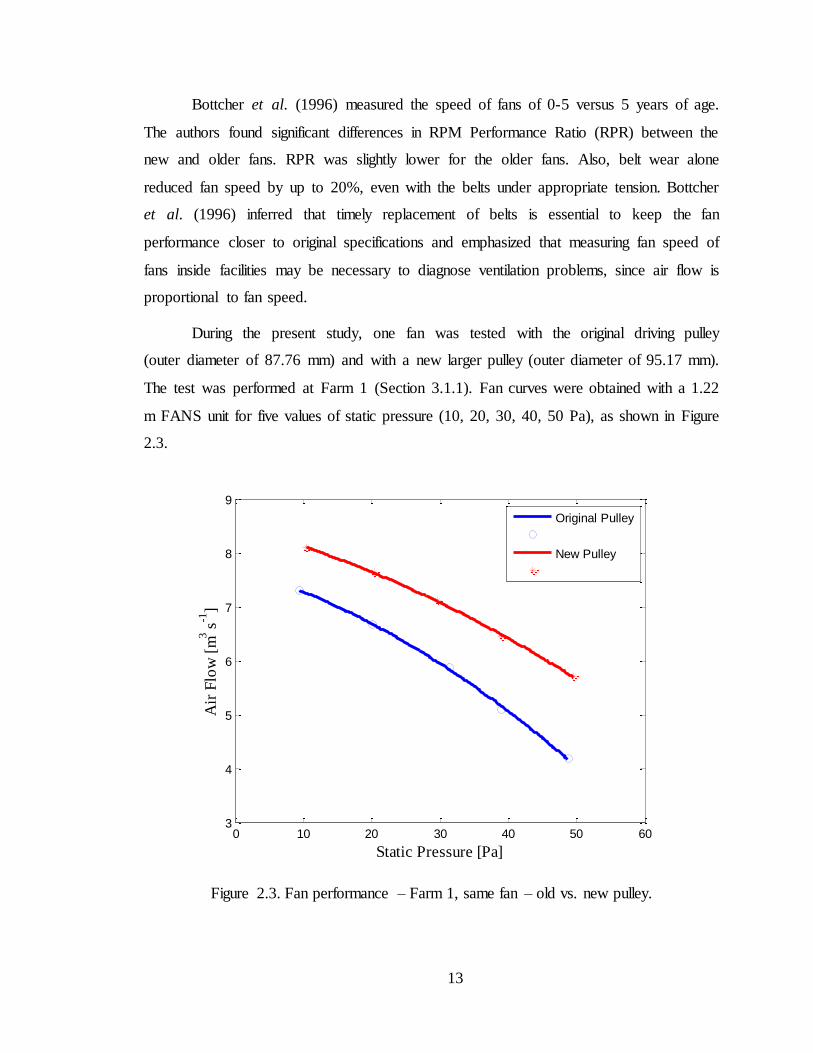
During the present study, one fan was tested with the original driving pulley
(outer diameter of 87.76 mm) and with a new larger pulley (outer diameter of 95.17 mm).
The test was performed at Farm 1 (Section 3.1.1). Fan curves were obtained with a 1.22
m FANS unit for five values of static pressure (10, 20, 30, 40, 50 Pa), as shown in Figure
2.3.
Figure 2.3. Fan performance – Farm 1, same fan – old vs. new pulley.
0 10 20 30 40 50 603
4
5
6
7
8
9
Static Pressure [Pa]
Air
Flo
w [
m3 s
-1]
Original Pulley
New Pulley
14
The new driving pulley was larger than the original one, thus the diameter ratio
between the new driving pulley and the driven pulley was reduced, thus increasing the
fan rotational speed. Test results showed that the fan moved approximately 20.2 ± 8.9 %
more air with the larger driver pulley than it did with the original pulley for all values of
static pressure measured. Also, the fan rotated 8.98 ± 0.08 % faster with the larger driver
pulley for all values of static pressure measured. Despite the drop in fan efficiency,
increase in motor wear and possible safety issues related to the pulley replacement, the
fan capacity was improved and, for this reason, the producer replaced the original driving
pulley with the larger one. Ventilation rate information in this type of situation should
only be measured in-situ, once the manufacturer fan performance data is no longer
applicable to this fan.
2.4 Alternative Methods for Measuring Ventilation Rate or Fan Air Flow in -situ.
Lima et al. (2010) evaluated negative and positive pressure ventilation systems in
poultry buildings. The author studied the litter quality, environmental conditions, as well
as ammonia and carbon dioxide emissions from poultry barns equipped with either
ventilation system. Fan ventilation rate was obtained through the traverse method
(ASHRAE, 2005), using a hot-wire anemometer. Lacey et al. (2003) studied particulate
matter and ammonia emission factors for tunnel ventilated broiler houses and used a vane
thermo–anemometer (451126, Extech, Waltham, Mass.) to measure building ventilation
rates. However, velocity rates were not obtained at the fan cross sections, but from 15
points across the building section, 40 m from the house exhaust end.
The fan traverse method consists of a straight average of individual point
velocities measured in the center of equal areas over the plane through which the air is
flowing. The velocities can be determined by the Log – Tchebycheff (log-T) rule, which
is recommended for rectangular ducts, or by the equal – area method (ASHRAE, 2005).
When using the Log – T rule in a rectangular duct, a minimum of 25 measurement points
should be used, whereas for a circular duct the Log-Linear method should be used at
three symmetrically disposed diameters. The traverse measurement may be performed

15
with various types of anemometers. This method is effective, however it requires time
and implies labor to measure air velocities at many different points.
The hot-wire anemometer consists of a Thermal Resistance Device (RTD),
thermocouple junction or thermistor sensor enclosed within the end of a probe
(ASHRAE, 2005). Hot – wire anemometers measure air velocity directly and are able to
sense low air velocities (from 0 to 0.51 m s-1) with a typical accuracy of 2 to 5% over the
entire velocity range. However, the hand–held type of hot-wire anemometer has a few
limitations for its use in the field. The unidirectional sensor, for example, must be
carefully aligned in the air stream to achieve accurate results. Also, the sensor must be
kept clean, since its calibration can be compromised by dirt or contaminants. Although
the sensor provides a high speed response, there may be fluctuating velocity
measurements for turbulent flows.
Vane anemometers are light wind-driven wheels connected through a gear train to
a set of recording dials that read linear distance of air passing during a period of time
(ASHRAE, 2005). This type of anemometer is available in different sizes and each one
requires individual calibration. This type of anemometer has limitations at low air
velocities. Many vane anemometers have starting speeds of 0.25 m s-1 and do not sense
extremely low air velocities as well as the hot-wire anemometer.
Demmers et al. (1999) evaluated ammonia emissions from two mechanically
ventilated livestock buildings in the UK. A tracer gas (CO) method was used for
measuring ventilation rates from naturally ventilated livestock buildings. The ventilation
rates were compared to the rates estimated using fan wheel anemometers and significant
correlations were found between the estimated ventilation rate using the tracer method
and the measured ventilation rate using fan wheel anemometers.
The tracer gas method is performed by introducing a known mass of tracer into a
building and estimating the ventilation rate using the equation of conservation of mass
(Equation 2.2, Demmers et al., 1999).
( ) ( )
( ) ( ) Equation 2.2
16
Where,
Q(t) = Ventilation rate;
φp (t) = Tracer production rate;
Ci(t) = Internal tracer concentration;
Ce(t) = Background tracer concentration.
Demmers et al. (1999) chose carbon monoxide (CO) as a tracer gas, because its
density is similar to air density, it is reasonably chemically inert and has a low
background concentration. Also, an introduced tracer provides more accurate ventilation
rates than tracers resulting from animal metabolic activities, such as carbon dioxide or
heat. Although the authors found ventilation rates to be 6 to 12% underestimated
compared to the direct method of measuring air flow rate, this variation is generally
accepted for the gas tracer method of estimating building ventilation.
The difficulties with this method include keeping the CO concentrations within
maximum allowable and minimum measurable limits, identifying all air inlets and outlets
in the buildings, delayed response in CO concentrations to changes in the CO release and
to variation in the ventilation rate. Also, perfect air mixing in the building is assumed to
use the gas tracer method, which can result in uncertainty in the calculation of ventilation
rates.
Maghirang et al. (1998) evaluated a freely rotating propeller to measure fan air
flow rates in livestock buildings. The device consisted of two 20 cm blades that rotated
freely in proportion to the flow rate moved by test fans. A photoelectric sensor was
placed on each blade to measure the rotational speed of the impeller, while a power
supply/display unit monitored and recorded the measured speeds. The impeller device
was validated in a wind tunnel test chamber constructed according to the Air Movement
and Control Association AMCA Standard 210-85 and air flow was regressed as a linear
function of the impeller rotational speed.
Strong relationships between air flow and impeller rotational speed were obtained
in the laboratory. Still, care should be taken when using this device to test fans in – situ.
17
Reductions in performance of test fans of up to 12.8% were found during the field tests.
These reductions were related to the size of test fans and to static pressure conditions,
when the impeller was placed next to the intake of a test fan. According to the authors,
reduction in air flow can be accounted for the pressure loss associated with the impeller
and by the restriction in air flow associated with the duct where the impeller was
mounted. The authors, therefore, suggested that larger diameter ducts could be used to
minimize pressure loss during fan tests. On the other hand, placing the impeller device on
the discharge side of the test fan tended to increase the air flow moved by 41cm and
51cm fans in up to 11.8%.
2.5 Measuring Ventilation Rate - FANS Unit
2.5.1 Design Features
The FANS (Fan Assessment Numeration System) Unit is a device that was
developed to measure fan performance in-situ. Testing a fan in-situ provides the actual
fan performance as it is installed and operating with all accessories in place. The FANS
unit was invented by the URSDA-ARS Southern Poultry Research Laboratory (Simmons
et al., 1998) and refined at University of Kentucky (Gates et al., 2004, Sama et al., 2008).
The 1.22 m FANS unit has an array of five propeller anemometers (Gill Propeller
Anemometer, model 27106T, R. M. Young Company) mounted on a horizontal bar that
travels upward and downward measuring air speed of fans up to 1.37 m in diameter. The
anemometers consist of four 20 cm blades made of carbon fiber thermoplastic. The
propeller anemometer operational range is 0 – 40 m s-1 for axial flow and 0 – 35 m s-1 for
all angles flow, with an accuracy of ± 1%.
The array of propeller anemometers is located on a rectangular bar constructed
from 25.4 mm square tubing with a 1.6 mm wall thickness (Gates et al., 2002). The array
is supported on vertical traverses consisting of dual rail linear bearings connected to
rotating lead screws. One of the screws is driven by a gear motor, while the second screw
is driven by a chain, which connects both screws. The side frame sections are identical
and have vertical square tubes on the inside section that support the traverses, through

18
holes drilled every 50 mm (1.97 in). On the outside section of the side frames, there are
4.8 mm (3/16 in) thick aluminum plates with attached carry handles to facilitate the
transport of the FANS unit. The bottom and top frames have tubing for mounting the
control box and motor, as well as a chain tensioner, respectively (Gates et al., 2002).
The front section of the frame was faced with a curved surface, made of 0.4547
mm aluminum sheets (26 gauge) to promote a smooth air flow entrance with low
dynamic loss (Gates et al., 2002) through the FANS unit. The motor output shaft located
near the bottom frame of the FANS unit was joined to the vertical screw via flexible
coupling. Figure 2.4 and Figure 2.5 show the FANS unit assembled with all the
components previously described.
Figure 2.4. Back view of the 1.22 m (48 in) FANS unit set up near the discharge side of the fan: a. Screw, b. Vertical traverse, c. Motor, d. Control box, e. Array with
propeller anemometers, f. Carry handle, g. Chain drive.
a b
c
e
f
d
g

19
Figure 2.5. Front view of the 1.22 m (48 in) FANS unit set
up next to the intake side of an exhaust fan.
The motor (Figure 2.4) runs the screw which moves a sprocket, which moves the
chain located on the top frame. The chain, in turn, moves the other screw on the opposite
side frame. Therefore, both screws rotate at the same speed, making the array travel up
and down in a horizontal position. More information and details about the FANS unit
design and calibration can be found in Simmons et al. (1998b), Gates et al. (2002), Gates
et al. (2004) and Sama et al. (2008).
2.5.2 Fan Test and Data Acquisition
Five thousands samples of air velocity are acquired per second from each of the
five analog inputs of the anemometers (Sama et al., 2008), while the array traverses from
one limit switch to the other (bottom or top of FANS), during a fan test using a 1.22 m
FANS unit. These samples are averaged and result in approximately 1340 averaged
velocity readings, uniformly distributed across the FANS section. These readings

20
comprise one test, which lasts about 185 seconds. The FANS computer software
calculates a total average air speed during a fan test and multiplies it by the FANS
opening area, which produces an average air flow through the FANS unit during a
performance test.
FANS software was developed specifically to operate FANS units. The most
updated version of the FANS unit software is FANS Interface 1.4.0.1 (2010), written in
VisualBasic and developed at the Biosystems and Agricultural Engineering Department
at the University of Kentucky. Figure 2.6 shows the FANS User Interface 1.4.0.1.
Figure 2.6. FANS Interface 1.4.0.1, Biosystems and Ag. Engineering Department,
University of Kentucky.
A fan test is started by clicking on the button “Run Test” shown in Figure 2.6.
After clicking on “Run Test”, the array will travel up or down towards the limit switch,
while the propeller anemometers measure air speed. The array can be stopped, raised or
lowered, if desired. When the test is done, approximately 185 seconds after its start, the
interface will show an average air flow measured during the entire test in the box “Air
Flow”. Also, the average static pressure will be given in the box “Δ Pressure”. The test
results of air flow and static pressure, as well as averaged values of voltage output from
each anemometer are automatically saved in a Comma Separated Value data file during
the test. Environmental conditions, such as temperature, barometric pressure and relative

21
humidity can be added in the respective boxes, shown in Figure 2.6, and thus
automatically saved in the same file. However, the environmental measurements must be
performed separately from the FANS unit (Sub-section 3.3.3.5).
2.5.3 Use of the FANS unit
Casey et al. (2007) reported that a principal source of uncertainty in measuring air
emissions has to do with measurement of the building ventilation rates, since effects such
as harsh environment, fan maintenance, wind effects and others make the ventilation rate
measurement difficult even for mechanically ventilated buildings. The authors studied the
repeatability when using FANS unit to measure air flow of ventilation fans. Also, fan
tests were performed at the fan test chamber at the University of Illinois
Bioenvironmental and Structural Systems (BESS) Laboratory, with and without the
FANS unit. Fan performance curves obtained when the FANS unit was present were
compared with fan performance curves obtained when there was no FANS unit near the
test fan.
The authors found that the FANS unit is very repeatable in its determination of air
flow rate and there does not appear to be any need to conduct repeated measurements.
The FANS unit induced an air flow penalty of 2% only on 1.22 m diameter Chore Time
Turbo fans (38233-2) used in the study at static pressure lower than 30 Pa. However, the
authors reported that there was no penalty associated with the FANS unit when testing
fans with diameters of 0.91 m or less and 1.22 m diameter fans with capacities of less
than 34.000 m3 h-1.
Jacobson et al. (2001) measured baseline emission rates of odor, ammonia,
hydrogen sulfide, carbon dioxide and particulate matter from six types of livestock
buildings located at different states. The authors emphasized that measuring ventilation
rate is critical for estimating building emission rates. The ventilation rates used in this
study were obtained by using the fan status (on/off), static pressure measurement and
with the ventilation capacity of the fans located in the barns, obtained with a FANS unit.

22
Hoff et al. (2004) evaluated the hydrogen sulfide, ammonia, PM10 and odor
emissions from swine and poultry houses in six regions throughout the United States. The
authors mentioned that the gas tracer method of estimating the building ventilation rate,
although long recognized and used for years, suffers from inaccuracy when there is
incomplete air mixing in the building and is very instrument intensive. Therefore, Hoff et
al. (2004) reported that the gas tracer method is not accurate enough for emission studies
and opted to use a FANS unit to measure performance of ventilation fans during this
study.
Gates et al. (2005) proposed a method for measuring ammonia emissions from
broiler and layer barns, which suggested the direct measurement of ventilation rate using
the FANS unit and the CO2 balance method for larger layer houses. The suggested
method of estimating ammonia emissions has been successfully used to establish baseline
values for the U.S.A. The authors calculated that if the direct measurement of ventilation
rate using the FANS unit was not used, the building emission rate could be overestimated
up to approximately 17.5% using BESS laboratory data for fan tests. The cause of the
differences between the ventilation rates obtained from in-situ measures and ventilation
rates obtained in the laboratory was mainly attributed to installation, operation and
maintenance factors (Gates et al. 2005).
Several factors cause fan performance to degrade over time, such as dust and dirt
accumulation on the blades and belt wear (Bottcher et al., 1996). Casey et al. (2008)
reported up to 24% variation in fan performance attributed to accumulated dirt and
corrosion, resistances imposed by shutters, as well as motor and bearing wear due to run
time and aging. Janni et al. (2005) monitored sow gestation barns for emissions of
ammonia (NH3), carbon dioxide (CO2), hydrogen sulfide (H2S), odor, and particulate
matter 10 μm or less (PM10). Fan performances were obtained using a FANS unit and it
was found that the air flow was reduced by 30 to 60% when the fan drive belts were
slightly loose compared to the air flow obtained when the belts were properly tightened.
Gay et al. (2006) determined the ammonia emission rates in four tom turkey
houses (two brooder and two growout). The ventilation rates were obtained using the
FANS unit and fan run time data. All individual fans were tested with a FANS unit,
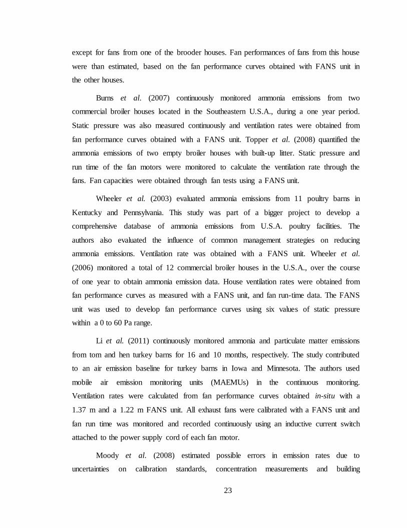
23
except for fans from one of the brooder houses. Fan performances of fans from this house
were than estimated, based on the fan performance curves obtained with FANS unit in
the other houses.
Burns et al. (2007) continuously monitored ammonia emissions from two
commercial broiler houses located in the Southeastern U.S.A., during a one year period.
Static pressure was also measured continuously and ventilation rates were obtained from
fan performance curves obtained with a FANS unit. Topper et al. (2008) quantified the
ammonia emissions of two empty broiler houses with built-up litter. Static pressure and
run time of the fan motors were monitored to calculate the ventilation rate through the
fans. Fan capacities were obtained through fan tests using a FANS unit.
Wheeler et al. (2003) evaluated ammonia emissions from 11 poultry barns in
Kentucky and Pennsylvania. This study was part of a bigger project to develop a
comprehensive database of ammonia emissions from U.S.A. poultry facilities. The
authors also evaluated the influence of common management strategies on reducing
ammonia emissions. Ventilation rate was obtained with a FANS unit. Wheeler et al.
(2006) monitored a total of 12 commercial broiler houses in the U.S.A., over the course
of one year to obtain ammonia emission data. House ventilation rates were obtained from
fan performance curves as measured with a FANS unit, and fan run-time data. The FANS
unit was used to develop fan performance curves using six values of static pressure
within a 0 to 60 Pa range.
Li et al. (2011) continuously monitored ammonia and particulate matter emissions
from tom and hen turkey barns for 16 and 10 months, respectively. The study contributed
to an air emission baseline for turkey barns in Iowa and Minnesota. The authors used
mobile air emission monitoring units (MAEMUs) in the continuous monitoring.
Ventilation rates were calculated from fan performance curves obtained in-situ with a
1.37 m and a 1.22 m FANS unit. All exhaust fans were calibrated with a FANS unit and
fan run time was monitored and recorded continuously using an inductive current switch
attached to the power supply cord of each fan motor.
Moody et al. (2008) estimated possible errors in emission rates due to
uncertainties on calibration standards, concentration measurements and building

24
ventilation rates. Gates et al. (2009) reported that the ventilation rate uncertainty
contributed to 78% and 98.9% of emission rate uncertainty for a 5% and 25% standard
uncertainty in fan ventilation rate measurement, respectively. Moody et al. (2008)
inferred that ventilation rate uncertainty is critical for controlling emission rate
uncertainty and the FANS unit contributed to reducing ventilation rate uncertainties.
Moody et al. (2008) emphasized that if less sophisticated methodologies were used to
estimate ventilation rate, the emission rate uncertainties could be substantially larger.
Therefore, researchers working under the US EPA (Environmental Protection Agency)
Air Consent Agreement adopted the FANS unit method to measure fan performance and
determine baseline emissions for dairy, swine and poultry houses.

25
CHAPTER 3
MATERIALS AND METHODS
3.1 Farms visited
Data were collected at five poultry barns in western Kentucky. Tests were
conducted with empty barns (between flocks), during the months of July through August,
2010. A total of ten 1.22 m diameter fans were tested at four farms operated by two
different poultry companies, designated as Poultry Company 1 and Poultry Company 2.
Five fans were tested in three different barns at Farm 1, under contract to Poultry
Company 1, while the other five fans were tested in one barn at each of Farms 2, 3 and 4,
all growout facilities for the Poultry Company 2. Additional information about the fans
tested in this study is available in Sub-sections 3.1.1 trough 3.1.4 of this chapter.
3.1.1 Farm 1 – under Contract to Poultry Company 1
A total of five fans were tested from three different barns (1, 2 and 3, Figure 3.1),
in Farm1, from Poultry Company 1.
Figure 3.1. Poultry barns at Farm 1, under contract to Poultry Company 1. Numbers 1,
2 and 3 designate Barns 1, 2 and 3 at Farm 1.
Each of the barns from Poultry Company 1 were 14 x 164 m, oriented East to
West, equipped with ten 1.22 m diameter Glass Pac Canada belt-driven fans (GP
48100299), placed immediately next to each other (Figure 3.2) on the sidewalls at the
2 3
1
26
exhaust end of the barn. The fans had plastic shutters, fiber glass housing and no
discharge cones. The motor information is given in Table 3.1.
Figure 3.2. Exhaust end of a representative barn at Farm 1 with exhaust fan placement illustrated. Fans were placed immediately
next to each other.
Table 3.1. Motor information for Glass Pac Canada fans.
Motor A O Smith
Model K56A25A78 Series 2098
Amperage 11/5.5 A
Voltage 115/230 V Power 1 HP
Speed 1725/1425 RPM
Figure 3.3 shows two additional fans on the exhaust end of a barn at Farm 1,
which were 1.32 m diameter Hired Hand Funnel Flow fans (FF-52-B-3F-SE-1.5S-246S-
0-0-VB), with butterfly dampers, fiber glass housing, and cones.
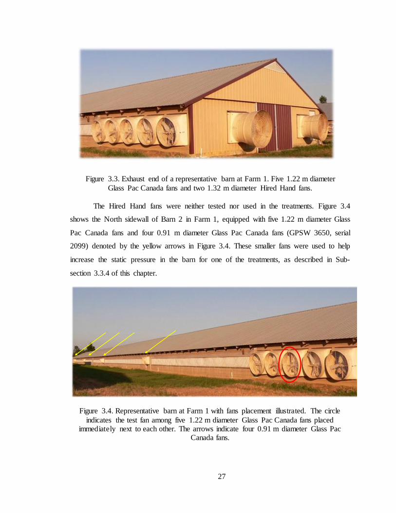
27
Figure 3.3. Exhaust end of a representative barn at Farm 1. Five 1.22 m diameter
Glass Pac Canada fans and two 1.32 m diameter Hired Hand fans.
The Hired Hand fans were neither tested nor used in the treatments. Figure 3.4
shows the North sidewall of Barn 2 in Farm 1, equipped with five 1.22 m diameter Glass
Pac Canada fans and four 0.91 m diameter Glass Pac Canada fans (GPSW 3650, serial
2099) denoted by the yellow arrows in Figure 3.4. These smaller fans were used to help
increase the static pressure in the barn for one of the treatments, as described in Sub-
section 3.3.4 of this chapter.
Figure 3.4. Representative barn at Farm 1 with fans placement illustrated. The circle
indicates the test fan among five 1.22 m diameter Glass Pac Canada fans placed immediately next to each other. The arrows indicate four 0.91 m diameter Glass Pac
Canada fans.

28
Fans tested inside barns 1, 2 and 3 from Farm 1 were all 1.22 m diameter Glass
Pac Canada fans located right in the center of each group of five exhaust fans, as
illustrated in Figure 3.4 and denoted by the red oval. The reason for choosing the fans
located at the center of each group of five fans for the fan testing was to allow all
treatments to be applied for the same fan. Table 3.2 shows the locations of each test fan,
inside barns from Poultry Company 1 (Farm 1).
Table 3.2. Position of test fans inside Farm 1, poultry barns in Kentucky – U.S.A.
Barn Fan tested Location
1 F1 South sidewall, third fan from the exhaust end of the barn F2 North sidewall, third fan from the exhaust end of the barn
2 F3 North sidewall, third fan from the exhaust end of the barn F4 South sidewall, third fan from the exhaust end of the barn
3 F5 North sidewall, third fan from the exhaust end of the barn
3.1.2 Farm 2 – under Contract to Poultry Company 2
A total of two fans were tested in barn 4, at Farm 2 under contract to Poultry
Company 2 (Figure 3.5).
Figure 3.5. Poultry barns from Farm 2, operated by Poultry Company 2. Number “4”
designates Barn 4 at Farm 2.
Farm 2, from Poultry Company 2, has four 13 x 166 m barns, oriented East to
West. Each barn is equipped with eight 1.22 m diameter belt driven Chore Time Turbo
Fans (38233-2) spaced 1.6 m apart (Figure 3.6) on the exhaust end sidewalls, with plastic
shutters, fiber glass housing and plastic cones. Table 3.3 contains information about the
fan motors.
4

29
Figure 3.6. Representative barn at Farm 2 with exhaust fan placement illustrated. Fans
were spaced 1.6 m from each other. The circle indicates the test fan.
Table 3.3. Motor information for Chore Time Turbo fans.
Motor General Electric
Industrial Systems
Model 5KCR49UN0462AT Amperage 4.4/5.1 A
Voltage 230 V Power 1 HP Speed 1725/1425 RPM
Motor capable of operating with two frequency supplies (60 and 50 Hz).
Figure 3.7 shows one additional fan on the exhaust end of a barn in Farm 2 from
Poultry Company 2, which was a 0.91 m diameter Chore Time fan, with plastic shutters,
fiber glass housing, and no cone. The 0.91 m diameter Chore Time fan was neither tested
nor used in the treatments.
Figure 3.7. Exhaust end of a representative barn at Farm 2. Four 1.22 m diameter Chore
Time Turbo fans and one 0.91 m diameter Chore Time fan.
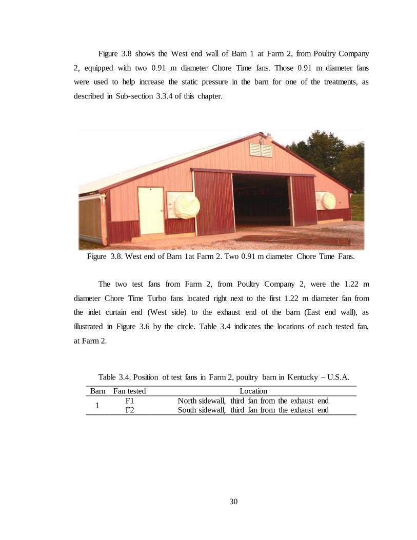
30
Figure 3.8 shows the West end wall of Barn 1 at Farm 2, from Poultry Company
2, equipped with two 0.91 m diameter Chore Time fans. Those 0.91 m diameter fans
were used to help increase the static pressure in the barn for one of the treatments, as
described in Sub-section 3.3.4 of this chapter.
Figure 3.8. West end of Barn 1at Farm 2. Two 0.91 m diameter Chore Time Fans.
The two test fans from Farm 2, from Poultry Company 2, were the 1.22 m
diameter Chore Time Turbo fans located right next to the first 1.22 m diameter fan from
the inlet curtain end (West side) to the exhaust end of the barn (East end wall), as
illustrated in Figure 3.6 by the circle. Table 3.4 indicates the locations of each tested fan,
at Farm 2.
Table 3.4. Position of test fans in Farm 2, poultry barn in Kentucky – U.S.A.
Barn Fan tested Location
1 F1 North sidewall, third fan from the exhaust end F2 South sidewall, third fan from the exhaust end
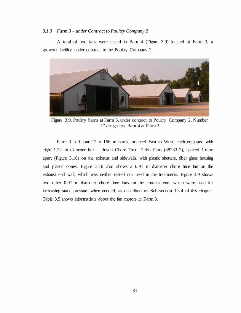
31
3.1.3 Farm 3 – under Contract to Poultry Company 2
A total of two fans were tested in Barn 4 (Figure 3.9) located at Farm 3, a
growout facility under contract to the Poultry Company 2.
Figure 3.9. Poultry barns at Farm 3, under contract to Poultry Company 2. Number
“4” designates Barn 4 at Farm 3.
Farm 3 had four 12 x 166 m barns, oriented East to West, each equipped with
eight 1.22 m diameter belt – driven Chore Time Turbo Fans (38233-2), spaced 1.6 m
apart (Figure 3.10) on the exhaust end sidewalls, with plastic shutters, fiber glass housing
and plastic cones. Figure 3.10 also shows a 0.91 m diameter chore time fan on the
exhaust end wall, which was neither tested nor used in the treatments. Figure 3.9 shows
two other 0.91 m diameter chore time fans on the curtains end, which were used for
increasing static pressure when needed, as described on Sub-section 3.3.4 of this chapter.
Table 3.5 shows information about the fan motors in Farm 3.
4

32
Figure 3.10. Exhaust end of a representative barn at Farm 3. Four 1.22 m diameter Chore
Time Turbo fans and one 0.91 m diameter Chore Time fan. 1.22 m diameter fans were spaced 1.6 apart. Red circle indicates test fan.
Table 3.5. Motor information for 1.22 m diameter Chore Time Turbo fans.
Motor General Electric
Industrial Systems
Model 5KCR49UN0462AT Amperage 4.4/5.4A
Voltage 230 V Power 1 HP
Speed 1725/1425 RPM
Motor capable of operating with two frequency supplies (60 and 50 Hz).
The two test fans in Farm 3 were 1.22 m diameter Chore Time Turbo fans located
right next to the first 1.22 m diameter fan from the tunnel curtains (West side) to the
exhaust end of the barn (East end wall), as indicated in Figure 3.10 by the red circle.
Table 3.6 shows the locations of each tested fan, in Farm 3.
Table 3.6. Position of test fans in Farm 3, poultry barn in Kentucky – U.S.A.
Barn Fan tested Location
4 F3 North sidewall, third fan from the exhaust end of the barn F4 South sidewall, third fan from the exhaust end of the barn

33
3.1.4 Farm 4 – under Contract to Poultry Company 2.
One fan (T5) was tested in Barn 3 (Figure 3.11) at Farm 3.
Figure 3.11. Poultry barns at Farm 4, under contract to Poultry Company 2. Number
“3” designates Barn 3 at Farm 4.
Farm 4 had three 13 x 164 m barns, oriented East to West, equipped with eight
1.22 m diameter Chore Time Turbo fans (38233-2) spaced 1.6 m apart (Figure 3.12) on
the exhaust end sidewalls, with plastic shutters, fiber glass housing and plastic cones.
Figure 3.11 shows two 0.91 m diameter Chore Time fans on the inlet curtain end, which
were used for increasing static pressure when needed, as described on Sub-section 3.3.4
of this Chapter. Table 3.7 contains information about the fan motors in Farm 4.
Figure 3.12. Representative barn at Farm 4 with exhaust fans placement illustrated. Fans
were spaced 1.6 m apart. The circle denotes the test fan.
3

34
Table 3.7. Motor information for Chore Time Turbo fans.
Motor General Electric Industrial Systems
Model 5KCR49UN0462AT Amperage 4.4/5.4 A Voltage 230 V
Power 1 HP Speed 1725/1425 RPM
Motor capable of operating with two frequency supplies (60 and 50 Hz).
The test fan (F5) from Poultry Company 2 Farm 4 was a 1.22 m diameter Chore
Time Turbo fan located right next to the first 1.22 m diameter fan from the curtain end
(East side) to the exhaust end of the barn (West end wall). F5 was located on the South
sidewall from the exhaust end.
3.2 FANS Unit Calibration
A 1.22 m FANS Unit (serial number: 48-0023) was calibrated in the
BioEnvironmental Structural Systems Laboratory (BESS Lab), Agricultural and
Biological Engineering, University of Illinois, Urbana, IL.
FANS calibration was performed by placing the FANS unit against the outlet face
of the BESS Lab chamber and sealing the gap between the chamber outlet and FANS unit
with Styrofoam (Figure 3.13). The tests were run within the static pressure range 0 to 62
Pa. Air flow was read by FANS unit once for each of the ten values of static pressure set
in the chamber. Also, air flow was calculated based on the pressure difference across
calibrated chamber nozzles for the ambient conditions of temperature, relative humidity
and barometric pressure, for every test run. Chamber air flow data were calculated based
on the ANSI/AMCA Standard 210-07 ANSI/ASHRAE 51-07, Laboratory Methods of
Testing Fans for Certified Aerodynamic Performance Rating.

35
Figure 3.13. FANS calibration being run in the BESS Lab
Chamber, Bioenvironmental and Structural Systems Laboratory,
University of Illinois, Urbana – IL.
Air flow obtained by the FANS unit was regressed as a linear function of the air
flow obtained from the BESS Lab chamber. The parameters obtained from the regression,
slope and intercept, were inserted into the FANS software.
Figure 3.14 illustrates the calibration curve for the 1.22 m FANS unit (serial
number: 48-0023).

36
Air Flow from BESS Chamber [m3 s
-1]
0 2 4 6 8 10 12 14 16
Air
Flo
w f
rom
FA
NS
Un
it [
m3 s-1
]
-2
0
2
4
6
8
10
12
14
16
Data
Linear Regression
95% Confidence Band
95% Prediction Band
Figure 3.14. 48-0023 FANS calibration.
The regression slope of 0.98 ± 0.004 and intercept of 0.08 ± 0.03 m3 s-1 from the
linear regression were added to the FANS unit software to correct the FANS air flow
readings. The FANS software used in this study (FANS Interface 1.4.0.0.1) has a specific
place where calibration information can be input, as shown in Figure 3.15. The slope and
intercept from the regression described were then input in the FANS software (Figure
3.15).
FANS Air Flow ± 0.05= 0.98 * BESS Air Flow - 0.08
R² = 0.99

37
Figure 3.15. FANS Interface 1.4.0.0.1 – calibration procedure.
The FANS software automatically inverted the regression to provide an air flow
reading as close as possible of the reference air flow (BESS Lab chamber air flow
output). The estimation of the real air flow is indicated by Equation 3.1, which is a
regression of the BESS Chamber air flow as a linear function of the FANS unit air flow.
RAF = Bo + B1 * FANS_AF Equation 3.1
Where,
RAF = Reference Air flow [m3 s-1] obtained from the BESS Lab Chamber;
Bo = Intercept = 0.0802 ± 0.0314 [m3 s-1];
B1 = Slope = 1.0207 ± 0.0040;
FANS_AF = FANS Air flow [m3 s-1].
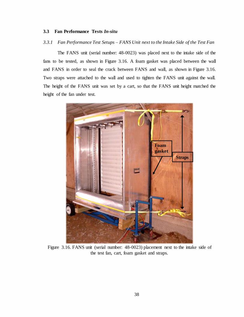
38
3.3 Fan Performance Tests In-situ
3.3.1 Fan Performance Test Setups – FANS Unit next to the Intake Side of the Test Fan
The FANS unit (serial number: 48-0023) was placed next to the intake side of the
fans to be tested, as shown in Figure 3.16. A foam gasket was placed between the wall
and FANS in order to seal the crack between FANS and wall, as shown in Figure 3.16.
Two straps were attached to the wall and used to tighten the FANS unit against the wall.
The height of the FANS unit was set by a cart, so that the FANS unit height matched the
height of the fan under test.
Figure 3.16. FANS unit (serial number: 48-0023) placement next to the intake side of
the test fan, cart, foam gasket and straps.
Foam
gasket
Straps

39
3.3.2 Fan Performance Test Setups – FANS Unit near the Discharge Side of the Test
Fan
The FANS unit was placed near the discharge side of the test fans and a sheet of
either 4 or 6 mil of polyethylene clear plastic was tightened around the fan and FANS
(Figure 3.17) with duct tape and a rope to provide a makeshift transition. Thus, all the air
moved by the fan passed through the FANS unit during the tests. A cart was used to
adjust the FANS to the test fan height.
Figure 3.17. FANS unit (serial number: 48-0023) near the discharge side of the test fan,
outside setup.

40
3.3.3 Fan Performance Test Setups – Readings Setup
3.3.3.1 Static Pressure Measurement
The white box located on the bottom of the FANS unit (Figure 3.18) contains a
differential pressure transducer (Setra Systems Model 265, series 0811) shown in Figure
3.19, which measures static pressure from 0 to 62 Pa (0 to 0.25 in H2O), with an
advertized accuracy of ± 1% FS (Full Span).
Figure 3.18. FANS unit (serial number: 48-0023) outside setup,
static pressure sensor.

41
Figure 3.19. Differential Pressure Transducer (Setra
Systems Model 265, series 0811)
Figure 3.20 shows an outlet for two hoses that connect with the static pressure
sensor. One hose goes inside the barn, while the other hose goes outside the barn. In this
way, the sensor could provide the difference in pressures from outside and inside the barn
during the tests.
Figure 3.20. Hoses on the FANS unit for static
pressure measurement.

42
The inside hose was placed approximately 12.2 m from the exhaust fans, during
all tests. The outside hose was placed about approximately 12.2 m from the exhaust end,
inside an open-top bucket to buffer the overall interference of the wind.
3.3.3.2 Air Flow and Static Pressure Readings
The air flow rate and static pressure were averaged during 185 second tests by
FANS Interface 1.4.0.0.1 software, developed at the University of Kentucky, Lexington,
U.S.A. A serial cable (Figure 3.21) connects the FANS unit to a computer (Figure 3.22),
where an average air flow and static pressure are calculated at the end of each test.
Figure 3.21. Serial cable connected to the FANS unit.
Figure 3.22. Reading through computer software.
The FANS user interface records approximately 1340 averaged air velocity
readings (Sub-section 2.5.2) that are automatically stored in comma separated type of
files that can be accessed after each fan test.
3.3.3.3 Power Readings
The visited farms were equipped with emergency backup generators that provide
electricity during power outage. Periodically these generators are exercised and tested as
part of their regular maintenance. A slight change in the magnitude of the power supply
can occur during these maintenance periods, which can change the fan speed. During the
fan tests, power, current, voltage and power factor at the fan motor were recorded in

43
order to verify if the supply conditions were about the same for all treatments. The power
readings also helped to determine if the electrical supply was from the transmission
system (grid) or if the farm generator was running.
The power monitoring was useful to assure that all the treatments within a farm
were done under the same conditions of electricity supply. Figure 3.23 shows the power
meter (AEMC single-phase, model 8230) used to record the power information during all
tests. Before the data collection, the AEMC power meter was sent to an authorized
laboratory for proper calibration.
Figure 3.23. Power Meter - AEMC PowerPad Jr, Model 8230. Corporate & Manufacturing
Address: Chauvin Arnoux®, Inc. d.b.a. AEMC® Instruments 15 Faraday Drive Dover,
NH 03820 U.S.A, http://www.aemc.com/.
Two extension power cords were connected between the electrical outlet and the
fan plug, as indicated by the arrows in Figure 3.24. An improvised power cord was
installed in the fan-supply circuit with plugs to accommodate voltage probes and to
facilitate the use of an amperage clamp, as shown in Figure 3.25. The power meter
recorded averages of power (watts), current (amperes), voltage (volts) and power factor at
one minute intervals during all tests.

44
Figure 3.24. Power cords. Arrow 1 indicates the extension cord between the power
supply and power meter. Arrow 2 indicates the extension power cord between the power
meter and the fan.
The power cords re-routed the electricity supply (Figure 3.24) to the power meter
(Figure 3.25) and back to the fan motor.
Figure 3.25. Setup of AEMC PowerPad Jr, Model 8230. The arrow indicates the
connector cord with separated wires for clamp-on measurements and spliced
connections for voltage probes.
1
2

45
3.3.3.4 Barn Air Speed Readings
Barn air speed (BS) was recorded at approximately 12 m from the tunnel fans, at
1.5 m height, using a Kestrel 4200, Pocket Air Flow Tracker (Figure 3.26). The air speed
measurements were done at three different spots across the barn section, spaced
approximately 2 m from the sidewalls and 4 m from each other, as illustrated in Figure
3.27.
Figure 3.26. Kestrel 4200, Pocket Air Flow Tracker (operational range
of 0 – 99.999,00 m3 h-1 ± 3.0%)
Figure 3.27. Barn Air Speed Measurements – 12 m from tunnel fans
at the height of the center of tunnel fans, 1.5 m, (not to scale).
Barn air speed was measured for all the treatments at all different static pressure
tested. Averages were calculated from measurements taken at the three locations
illustrated in Figure 3.27. The average barn air speed was tested as a dependent variable
to describe differences in air velocities obtained from anemometers 1 and 5 of the FANS
unit, as described in Section 4.3.
3.3.3.5 Other Measurements – Temperature, Barometric Pressure, Relative Humidity
The air conditions and fan speed were recorded during all tests and the barometric
pressure was read and recorded twice every test day approximately at 8:00 a.m. and 2:00
p.m. Figure 3.28 through Figure 3.30 show the temperature and humidity sensor
(Rotronic Hygroskop GT-1, temperature and relative humidity operational ranges of -
10oC – 50oC ± 0.3 o C/ 5% – 100% ± 2%, respectively) as well as the barometer
(Airguide Instrument Co.) and the tachometer (Monarch, Pocket Tach. 10, operational
range of 5 RPM – 100.000 RPM ± 1 RPM).

46
Figure 3.28. Temperature/Humidity sensor
- Rotronic Hygroskop GT-1 Rotronic Instrument Corp. 135
Engineers Rd Suite 150
Hauppauge NY,11788
Figure 3.29. Barometer Airguide
Instrument Co.
Figure 3.30. Tachometer, Monarch
Pocket Tach 10
Monarch Instrument 15 Columbia Drive
Amherst, NH, 03031.
The Rotronic Hygroskop had the temperature checked against a mercury
thermometer inside an insulated container and the humidity sensor was calibrated using
saline humidity standards. All the treatment comparisons were done for the same values
of static pressure, therefore the air density was not corrected for standard values.
3.3.4 Fan Performance Test - Procedure
An array of five propeller anemometers (Figure 3.31) are attached to a rack that
traveled up and down during a fan performance test, measuring air speeds continuously in
real-time. Computer software calculated the average air flow, from approximately 1340

47
averaged air velocity readings obtained during the traverse measurement for each single
run with the FANS unit (Gates et al., 2004 and Sama et al., 2008).
A traverse test was run for all treatments for each of eight static pressures set for
the treatment within the range 0 to 60 Pa. This data was used to build fan performance
curves of air flow versus static pressure. The static pressure (SP) step within the range 0
to 60 Pa was dependent on the minimum static pressure that could be established in the
building for each treatment. Static pressure was set by opening and closing the inlet
curtains and by energizing 0.91 m diameter fans on the inlet curtain end of the barn when
higher static pressures were needed.
Figure 3.31. FANS unit (serial number: 48-0023), anemometer propellers.
3.4 Experiment Protocol
The fan under test was selected mainly for its position on the sidewall and by
considering the desired combinations of fans to be operated for the treatments. One or
two fans were chosen for testing in each barn, as described in Section 3.1, to be tested

48
twelve times, once for each combination of operating fans (treatment). A total of ten 1.22
m diameter fans were tested. Six main treatment combinations were evaluated with the
FANS unit, when placed next to the intake side of the test fan and near the discharge side
of it, as described in Sub-section 3.4.1.
Five fans were tested at Farm 1 (under contract to Poultry Company 1), where
fans were placed immediately next to each other. Additionally five fans were tested at
Farms 2, 3 and 4 (under contract to Poultry Company 2) where fans were spaced 1.6 m
apart from each other. Data were treated as two different experiments, since there were
differences regarding the spaces between fans at Farm 1 (no space between fans) and fans
at Farms 2, 3 and 4 (spaced 1.6 m apart). Experiment 1 (E 1), therefore, was conducted
with fans placed immediately next to each other, at Farm 1, while Experiment 2 (E 2) was
conducted with fans spaced 1.6 m apart from each other, at Farms 2, 3 and 4.
3.4.1 Treatments
3.4.1.1 Treatments to Satisfy Objective 1 – Treatments “P” (operating fan positions
relative to FANS unit and test fan).
- Upstream treatment: FANS unit and test fan upstream from adjacent
operating fans (Figure 3.32);
- Downstream treatment: FANS unit and test fan downstream from
adjacent operating fans (Figure 3.33);
- Middle treatment: FANS unit and test fan between adjacent operating
fans (Figure 3.34);
- Test Fan Alone treatment: Test fan operating alone – no other exhaust
fans operating (Figure 3.35);
- Same Sidewall: Operating fans on the same sidewall as the FANS unit
and test fan (Figure 3.36);
- Opposite Sidewall: Operating fans on the opposite sidewall from the
FANS unit and test fan (Figure 3.37);
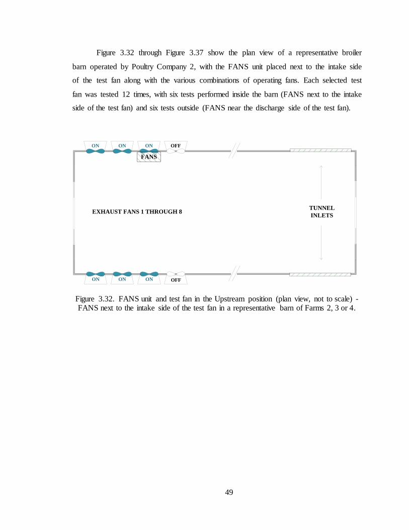
49
Figure 3.32 through Figure 3.37 show the plan view of a representative broiler
barn operated by Poultry Company 2, with the FANS unit placed next to the intake side
of the test fan along with the various combinations of operating fans. Each selected test
fan was tested 12 times, with six tests performed inside the barn (FANS next to the intake
side of the test fan) and six tests outside (FANS near the discharge side of the test fan).
TUNNEL
INLETSEXHAUST FANS 1 THROUGH 8
FANS
ON OFF
OFF
ONON
ON ON ON
Figure 3.32. FANS unit and test fan in the Upstream position (plan view, not to scale) - FANS next to the intake side of the test fan in a representative barn of Farms 2, 3 or 4.

50
TUNNEL
INLETSEXHAUST FANS 1 THROUGH 8
FANS
ON
ON
OFFOFF ON
OFF OFF ON
Figure 3.33. FANS unit and test fan in the Downstream position (plan view, not to scale)
- FANS next to the intake side of the test fan in a representative barn of Farms 2, 3 or 4.
TUNNEL
INLETSEXHAUST FANS 1 THROUGH 8
FANS
ON
ON
OFF ON
OFF ON
ON
ON
Figure 3.34. FANS unit and fan test in the Middle position (plan view, not to scale) - FANS next to the intake side of the test fan in a representative barn of Farms 2, 3 or 4.
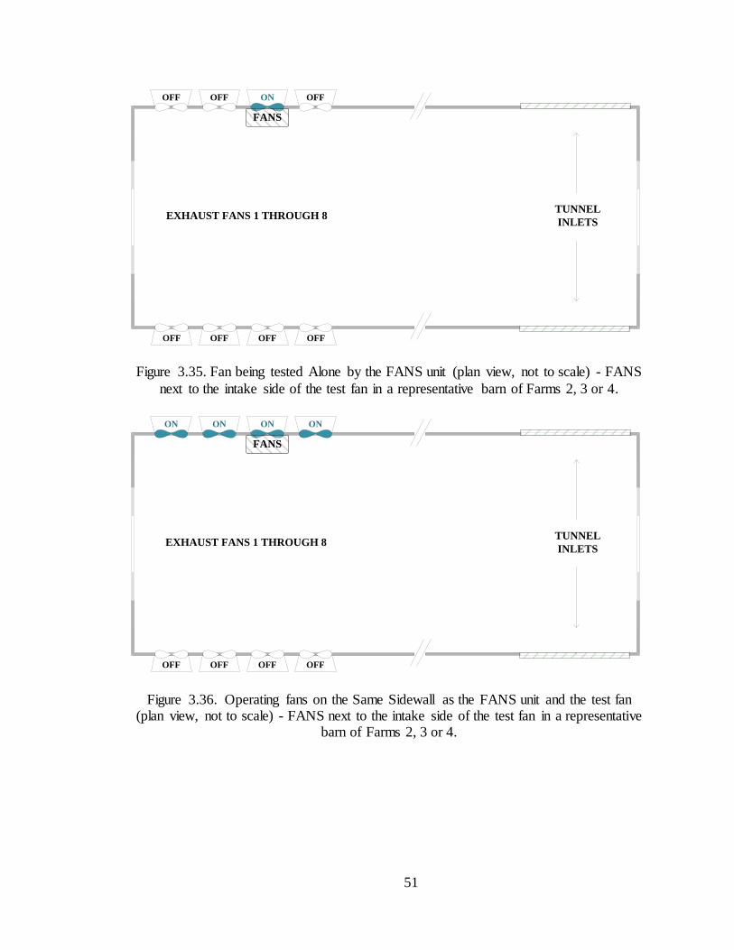
51
TUNNEL
INLETSEXHAUST FANS 1 THROUGH 8
FANS
ONOFF OFF OFF
OFF OFF OFF OFF
Figure 3.35. Fan being tested Alone by the FANS unit (plan view, not to scale) - FANS
next to the intake side of the test fan in a representative barn of Farms 2, 3 or 4.
TUNNEL
INLETSEXHAUST FANS 1 THROUGH 8
FANS
ON ON
OFF
ONON
OFF OFF OFF
Figure 3.36. Operating fans on the Same Sidewall as the FANS unit and the test fan (plan view, not to scale) - FANS next to the intake side of the test fan in a representative
barn of Farms 2, 3 or 4.

52
TUNNEL
INLETSEXHAUST FANS 1 THROUGH 8
FANS
ON
OFF
OFF OFF OFF
ON ON ON
Figure 3.37. Operating fans on the Opposite Sidewall from the FANS unit and the test
fan (plan view, not to scale) - FANS next to the intake side of the test fan in a representative barn of Farms 2, 3 or 4.
o Treatment “P” Specifications:
The previous images describing the treatments represent barns operated by
Poultry Company 2, containing a total of eight 1.22 m diameter exhaust fans, whereas the
barns operated by Poultry Company 1 had ten 1.22 m diameter exhaust fans. Therefore,
some treatments in Experiment 1 and Experiment 2 differed in the number of operating
fans. The treatment specifications for each farm are presented in Table 3.8.
Table 3.8. Treatment specifications.
Treatments Farm from Poultry
Company 1
Farms from Poultry
Company 2
Test Fans
Location
Number
of Fans
Operating on
Treatment
Test Fans
Location
Number
of Fans
Operating on
Treatment
Upstream
Centered - 3rd from the
exhaust end of the barns.
6
Not Centered –
3rd from the exhaust end of the barns.
6
Downstream 6 4 Middle 6 6 Alone 1 1
Same
Sidewall 5
4
Opposite
Sidewall 5
4

53
The treatments that differed in barns from Poultry Company 1 and Poultry
Company 2 were “Downstream”, “Same Sidewall” and “Opposite Sidewall”, as shaded
in Table 3.8. Figure 3.38 through Figure 3.40 illustrate these treatment configurations for
fans tested inside barns in Farm 1, operated by Poultry Company 1.
TUNNEL
INLETSEXHAUST FANS 1 THROUGH 10
FANS
ON
ON
OFFOFF ON
OFF OFF ON
ON
ON
Figure 3.38. FANS unit and test fan in the Downstream position (plan view, not to scale)
- FANS next to the intake side of the test fan in a representative barn of Farm 1.

54
TUNNEL
INLETSEXHAUST FANS 1 THROUGH 10
FANS
ON ON
OFF
ONON
OFF OFF OFF
ON
OFF
Figure 3.39. Operating fans in the Same Sidewall as the FANS unit and the test fan (plan
view, not to scale) - FANS next to the intake side of the test fan in a representative barn of Farm 1.
TUNNEL
INLETSEXHAUST FANS 1 THROUGH 10
FANS
ON
OFF
OFF OFF OFF
ON ON ON ON
OFF
Figure 3.40. Operating fans in the Opposite Sidewall from the FANS unit and the test fan (plan view, not to scale) - FANS next to the intake side of the test fan in a representative
barn of Farm 1.
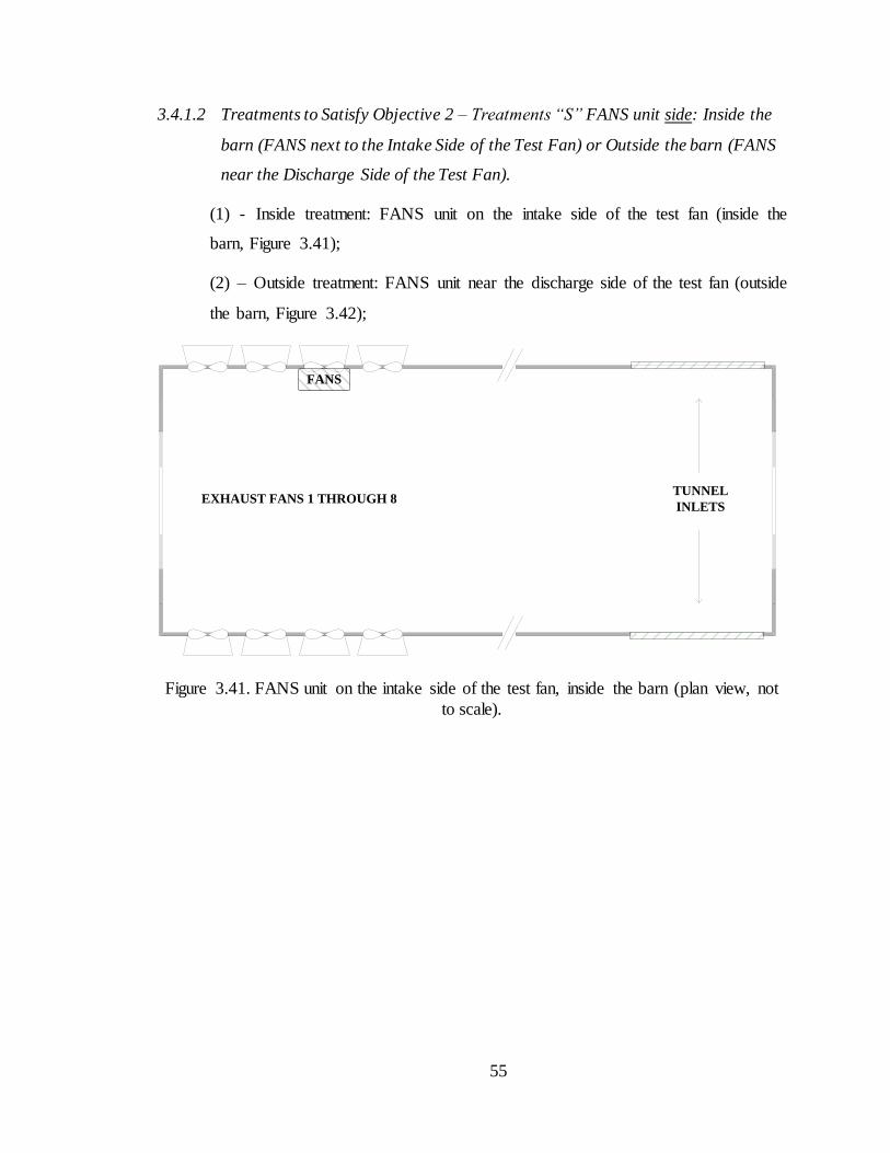
55
3.4.1.2 Treatments to Satisfy Objective 2 – Treatments “S” FANS unit side: Inside the
barn (FANS next to the Intake Side of the Test Fan) or Outside the barn (FANS
near the Discharge Side of the Test Fan).
(1) - Inside treatment: FANS unit on the intake side of the test fan (inside the
barn, Figure 3.41);
(2) – Outside treatment: FANS unit near the discharge side of the test fan (outside
the barn, Figure 3.42);
TUNNEL
INLETSEXHAUST FANS 1 THROUGH 8
FANS
Figure 3.41. FANS unit on the intake side of the test fan, inside the barn (plan view, not
to scale).
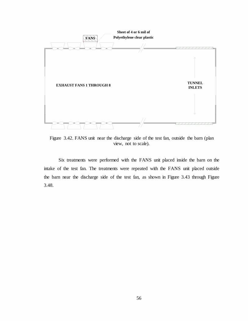
56
TUNNEL
INLETSEXHAUST FANS 1 THROUGH 8
FANS
Sheet of 4 or 6 mil of
Polyethylene clear plastic
Figure 3.42. FANS unit near the discharge side of the test fan, outside the barn (plan view, not to scale).
Six treatments were performed with the FANS unit placed inside the barn on the
intake of the test fan. The treatments were repeated with the FANS unit placed outside
the barn near the discharge side of the test fan, as shown in Figure 3.43 through Figure
3.48.

57
TUNNEL
INLETSEXHAUST FANS 1 THROUGH 8
FANS
ON OFF
OFF
ONON
ON ON ON
Figure 3.43. FANS unit and test fan in the Upstream position (plan view, not in scale) – FANS unit near the discharge side of the test fan in a representative barn of Farms 2, 3 or
4.
TUNNEL
INLETSEXHAUST FANS 1 THROUGH 8
FANS
ON
ON
OFFOFF ON
OFF OFF ON
Figure 3.44. FANS unit and test fan in the Downstream position (plan view, not to scale) – FANS unit near the discharge side of the test fan in a representative barn of Farms 2, 3
or 4.

58
TUNNEL
INLETSEXHAUST FANS 1 THROUGH 8
FANS
ON
ON
OFF ON
OFF ON
ON
ON
Figure 3.45. FANS unit and test fan in the Middle position (plan view, not to scale) –
FANS unit near the discharge side of the test fan in a representative barn of Farms 2, 3 or 4.
TUNNEL
INLETSEXHAUST FANS 1 THROUGH 8
FANS
ONOFF OFF OFF
OFF OFF OFF OFF
Figure 3.46. Fan being tested Alone by the FANS unit (plan view, not to scale) – FANS unit near the discharge side of the test fan in a representative barn of Farms 2, 3 or 4.

59
TUNNEL
INLETSEXHAUST FANS 1 THROUGH 8
FANS
ON ON
OFF
ONON
OFF OFF OFF
Figure 3.47. Operating fans on the Same Sidewall as the FANS unit and test fan (top
view, not to scale) – FANS unit near the discharge side of the test fan in a representative barn of Farms 2, 3 or 4.
TUNNEL
INLETSEXHAUST FANS 1 THROUGH 8
FANS
ON
OFF
OFF OFF OFF
ON ON ON
Figure 3.48. Operating fans on the Opposite Sidewall from the FANS unit and the test fan (top view, not to scale) – FANS unit near the discharge side of the test fan in a
representative barn of Farms 2, 3 or 4.
60
3.4.1.3 Satisfying Objective 3
Objective 3 was to evaluate if the FANS unit is the cause of possible differences
on fan performance results. Fan performance results are expected not to be significantly
different from each other when placing the FANS Unit on the intake side of the test fan
as compared to placing the FANS unit near the discharge side of the test fan (Li et al.,
2009). Therefore, if fan test results behave differently among the “P” treatments when the
FANS unit is placed next to the intake side of the test fan (Inside treatment) as compared
to placing the FANS unit near the discharge side of the fan (Outside treatment), it can be
concluded that the FANS unit causes possible air flow penalties during fan performance
tests. Thus, the approach used to satisfy objective 3 was to evaluate the interaction of
objectives 1 and 2.
3.4.1.4 Air Flow Readings per Treatment
Eight static pressures were set in the poultry barns for each treatment and one
value of air flow was obtained with the FANS unit and recorded for each of the eight
static pressure values. The ambient air conditions (Sub-section 3.3.3.5) during the tests,
as well as power information (Sub-section 3.3.3.3) and barn air speed (Sub-section
3.3.3.4) were recorded for each test run.
3.5 Experimental Design
Data gathered at the two different types of barn (with exhaust fans spaced 1.6 m
apart or not spaced) were treated as two different experiments owing to the fact that
treatments were not exactly the same from one experiment to the other. Treatments had
different numbers of fans operating from one farm to the other, as shown in Table 3.8.
Also, poultry barns operated by Poultry Company 1 had fans placed immediately next to
each other, while the barns operated by Poultry Company 2 had fans spaced 1.6 m apart
from each other.
Experiment 1(E 1) was carried out at Farm 1, operated by Poultry Company 1,
where the barns were equipped with ten 1.22 m diameter fans placed immediately next to

61
each other (Figure 3.2). Experiment 2 (E 2) was carried out at Farms 2, 3 and 4, operated
by Poultry Company 2, where the barns were equipped with eight 1.22 m diameter fans
each placed 1.6 m apart from each other (Figure 3.6). The treatments were classified as a
2 (FANS inside or outside) x 6 (operating fan combinations) factorial arrangement.
Test fans were selected according to their position on sidewalls and the desired
combinations of operating fans for the treatments. Further, all fans inside a barn had to be
operating correctly, so that all treatments could be applied. The barns used for fan testing
were the ones available, which were not under cleaning or maintenance operations in
between flocks. Eight values of static pressure were tested per treatment per fan within
the range 0 to 60 Pa.
All treatments in an experiment were applied to all fans tested. Treatments were
applied to groups of eight experimental units, since each treatment was tested at eight
values of static pressure in the barn. In this study, fan was designated by the experiment
and fan numbers, for example: E2_F1 means fan 1(F 1) in Experiment 2 (E 2). Group of
experimental units were designated by the fan name and instance of fan test: E1_F2_I3
means fan 2 (F 2) in Experiment 1 (E 1) at instance 3 (I 3). Each experimental unit was
tested under one single condition of static pressure in the barn and received one single
treatment combination described in Sub-section 3.4.1. The total number of experimental
units was, therefore, 480 (96 per block) which is the number of treatment combinations
(12) multiplied by number of static pressure (8), multiplied by the number of blocks (5).
Treatment combinations 1 through 12 (6 x 2 factorial arrangement) were randomized
before being assigned to groups of experimental units.
The structure design of Experiments 1 and 2 was the Generalized Randomized
Complete Block (GRCB) design, in which the test fans were blocked in order to
minimize experimental error. Blocking the test fans allowed removing the variation
among fans from the experimental error. In this way, blocks contained one single fan, but
96 experimental units (eight groups of 12 fan-instances). Static pressure was used as a
covariate in the experiment. Using static pressure (SP) as a covariate in the statistical
model allowed the removal of the variation owing to the SP before estimating the
treatment effects on air flow (response variable), thus reducing experimental error. Figure

62
3.49 exemplifies the treatments application to group of experimental units within one
block in Experiment 1. The same structure design was applied to Experiment 2.
...E1_F1_I 1Block 1 (F1) E1_F1_I 2 E1_F1_I 12
SP 1, SP 2, … SP 8
Trt.
Combination 2
SP 1, SP 2, … SP 8
Trt.
Combination 1
SP 1, SP 2, … SP 8
Trt.
Combination 12
Block 2 (F2)
Block 3 (F3)
Block 4 (F4)
Block 5 (F5)
...E1_F2_I 1 E1_F2_I 2 E1_F2_I 12
SP 1, SP 2, … SP 8
Trt.
Combination 2
SP 1, SP 2, … SP 8
Trt.
Combination 1
SP 1, SP 2, … SP 8
Trt.
Combination 12
...E1_F3_I 1 E1_F3_I 2 E1_F3_I 12
SP 1, SP 2, … SP 8
Trt.
Combination 2
SP 1, SP 2, … SP 8
Trt.
Combination 1
SP 1, SP 2, … SP 8
Trt.
Combination 12
...E1_F4_I 1 E1_F4_I 2 E1_F4_I 12
SP 1, SP 2, … SP 8
Trt.
Combination 2
SP 1, SP 2, … SP 8
Trt.
Combination 1
SP 1, SP 2, … SP 8
Trt.
Combination 12
...E1_F5_I 1 E1_F5_I 2 E1_F5_I 12
SP 1, SP 2, … SP 8
Trt.
Combination 2
SP 1, SP 2, … SP 8
Trt.
Combination 1
SP 1, SP 2, … SP 8
Trt.
Combination 12
Figure 3.49. Layout of the GRCB design for E 1 with five blocks, eight SP`s (covariates), 12 groups of experimental units (represented by squares) with a total of 96 experimental
units per block, 6 x 2 treatment combinations and 40 replications. Same design structure was applied to E 2.
3.6 Statistical Analysis
Second order polynomial regressions were fitted to the data, using SAS® (9.2,
SAS Institute Inc., 2002-2008 Cary, NC, U.S.A), to represent the fan performance for
each treatment combination, for each fan (block). Bo, B1 and B2 represent the intercept,
linear and quadratic parameters of the curves. The form of the regression equation was:
AF(treatment) = Bo + SP * B1 + SP2 * B2 Equation 3.2

63
A Student t- test was performed to verify the hypothesis of the parameters being
significantly differently from zero, testing the significance of the polynomial relationship.
The differences between air flows provided in different treatments were calculated for the
same values of static pressure (SP), with the following equation:
Difference (%) = (AFtreatment ps(i) – AFtreatment ps(j))*100/AFtreatment ps(i) Equation 3. 3
Where,
p = Refers to treatment “P” (operating fans position relative to the FANS unit and
test fan), p = {Alone, Upstream, Downstream, Middle, Same Sidewall, Opposite
Sidewall};
s = Refers to treatment “S” (FANS near the intake or discharge side of the test
fan), s={Inside, Outside};
i,j i≠j, refers to distinct “p s” treatment combination;
AFtreatment ps = Predicted Air flow at the “p s” treatment combination [m3 s-1];
The significance of the differences among the treatments was tested through the
statistical model:
Y(hijl)k = µ + Fh + Pi + Sj + (P * S )ij+ SPl + E(hijl)k Equation 3.4
Where,
µ = overall mean considered common to all observations [m3 s-1];
Fh = random effect of the h-th block;
Pi = fixed effect on the i-th level of treatment “P”, i = {1,2,3,4,5,6}, FANS
position relative to operating fans;
Sj = fixed effect on j – th level of treatment “S”, j = {1,2}, FANS near the intake
(Inside treatment) or discharge side of test fan (Outside treatment);
SPl = fixed effect on the l – th level of SP reading, l = {1 through 8};
64
E(hijl)k = random component, which explains the random variation or experimental
error to the k-th experimental unit;
Y(hijl)k = air flow observation from the effect of the h-th block (fan), the l-th
covariate (SP), the i-th and j-th treatment effects, to the level of the k-th experimental
unit.
Pair wise comparisons were performed using the Least Significant Difference
(LSD) procedure, in order to identify differences between treatments. Proc Mixed of
SAS® (9.2, SAS Institute Inc., 2002-2008 Cary, NC, U.S.A) was used.

65
CHAPTER 4
RESULTS AND DISCUSSION
4.1 Experiment 1 (E1) – Fans from Poultry Company 1
Air flow rate obtained from each treatment was regressed as a second order
polynomial function of static pressure (SP), as described in section 3.6. The intercept,
first and second order parameters of the regressions are provided in Appendix A, Table
A.1. The addition of the quadratic term was significant at 90% confidence level for
approximately 83% of the regression curves. Therefore, the second order polynomial
regression was performed among all fan tests. The overall models of fan performance
were all significant at 95% confidence level and presented a strong second order
relationship between air flow rate and SP. Approximately 85% of the curves had a
coefficient of determination (R2) of at least 98% and overall p-value less than 0.0001.
The remaining fan curves presented an R2 of at least 95% and overall p-value less than
0.0004.

66
4.1.1 Fan Tests with the FANS Unit on the Intake Side of each Test Fan (Inside
Treatment)-Experiment 1
Figures 4.1 through 4.5 show the fan performance curves obtained in Experiment
1 (E 1), with the FANS placed next to the intake side (Inside treatment) of the test fans.
Figure 4.1. Fan performance curves, FANS unit Inside, E1_F1.
0 10 20 30 40 50 604
5
6
7
8
9
10
11
12
Static Pressure [Pa]
Air
Flo
w [
m3 s
-1]

67
Figure 4.2. Fan performance curves, FANS unit Inside, E1_F2.
Figure 4.3. Fan performance curves, FANS unit Inside, E1_F3.
0 10 20 30 40 50 604
5
6
7
8
9
10
11
12
Static Pressure [Pa]
Air
Flo
w [
m3 s
-1]
0 10 20 30 40 50 604
5
6
7
8
9
10
11
12
Static Pressure [Pa]
Air
Flo
w [
m3 s
-1]

68
Figure 4.4. Fan performance curves, FANS unit Inside, E1_F4.
Figure 4.5. Fan performance curves, FANS unit Inside, E1_F5.
0 10 20 30 40 50 604
5
6
7
8
9
10
11
12
Static Pressure [Pa]
Air
Flo
w [
m3 s
-1]
0 10 20 30 40 50 604
5
6
7
8
9
10
11
12
Static Pressure [Pa]
Air
Flo
w [
m3 s
-1]

69
Figure 4.1 through Figure 4.5 show that the fan performance curves differed from
each other among the treatments, for the tests with FANS inside the barn. The “P”
(position of operating fans relative to FANS and test fan) treatments had a significant
effect (p < 0.0001) on air flow test results. Generally, Alone and Middle treatments
presented the highest air flow results among the five test fans in Experiment 1 when the
FANS unit was placed next to the intake side of the test fan. The Alone treatment
significantly (p < 0.05) differed from the Downstream, Upstream and Opposite Sidewall
treatments.
The Upstream treatment produced significantly lower air flow values among the
same five test fans with FANS next to the intake side of the fans. All remaining “P”
treatments were significantly (p < 0.0001) different from the Upstream treatment. The
Downstream, Same Sidewall and Opposite Sidewall treatments were characterized by
intermediate fan performance curves, generally falling between the Alone/Middle and the
Upstream treatments. Downstream was significantly (p < 0.05) different from Middle and
Alone, whereas Opposite Sidewall was significantly different from Middle, Same
Sidewall and Alone. The differences between the “P” treatments were quantified and are
presented in Table 4.1.
Fan performance curves within the “P” treatments are not parallel, which
demonstrates that there was interaction between static pressure (SP) and “P” treatments
(p = 0.0018). The curves converged at higher SP values, as shown in Figure 4.1 through
Figure 4.5. The number of operating fans was the same for all the SP values measured at
each treatment. Therefore, the curves converged as the barn air speed was reduced. It is
suggested that a further study is performed in order to understand the relationship of air
velocities through the FANS unit and through the barn and air flow penalties.
Lim et al. (2010) evaluated the differences in air flow between a 1.22 m diameter
test fan operating freely and the same fan operating with a FANS unit on its intake side.
The authors found air flow rate reduction of approximately 3.0% from the original
laboratory fan test curve attributed to an air flow restriction caused by the FANS unit
structure. Similar to the results of Experiment 1 of this work, the authors found that the
air flow rate differences increased with lower static pressure values.

70
Average differences between treatments were calculated for low values of SP
(0<SP<30 Pa) and high values of SP (30 Pa < SP) for all tested fans, using Equation 3.3.
Table 4.1 presents averaged air flow differences between the treatments that were
significantly different from each other. The Least Square Means Difference procedure
was performed on SAS® for all values of SP to compare treatment combinations.
Negative differences mean that air flow from the first treatment in a paired comparison
was lower than air flow from the second compared treatment.
Table 4.1. Significant averaged differences in air flow rate between “P”
Treatments with the FANS unit next to the intake side of the test fan – Experiment 1.
Comparisons: Average Differences ± Std. Error
At Low SP`s
At High SP`s
Upstream vs. Alone -10.9% 2.0%
-6.8% 2.5% *
Upstream vs. Downstream -8.2% 3.1%
-6.2% 3.6% *
Upstream vs. Middle -10.3% 1.4%
-8.7% 3.2% *
Upstream vs. Same Sidewall -9.1% 1.9%
-7.1% 3.0% *
Upstream vs. Opp. Sidewall -8.0% 1.5%
-5.0% 1.9% *
Alone vs. Downstream 2.5% 2.3%
0.6% 2.1% **
Alone vs. Opp. Sidewall 2.7% 1.7%
1.7% 2.5% *
Opp. Sidewall vs. Middle -2.2% 1.4%
-3.5% 2.5% *
Opp. Sidewall vs. Same
Sidewall -1.0% 1.2%
-2.0% 3.0% **
Downstream vs. Middle -2.0% -2.6%
-2.4% 3.7% **
* Significantly different at 99% confidence level (for both SP ranges); **
Significantly different at 95% confidence level (for both SP ranges).
Differences were calculated using Equation 3.3 and averaged for all tested
fans. Estimates of air flow [m3 s-1] can be found in Appendix B, Table B.3 (for both SP ranges).
Table 4.1 shows that the Upstream treatment was at least 8.0 ± 1.5% lower than
any other treatment, at low static pressures (0 < SP < 30 Pa). Differences between
Upstream and the other treatments were considered large enough to have a substantial
effect on the predicted barn ventilation. If all ten 1.22 m diameter fans were tested inside
a barn at 30 Pa using a FANS unit in the Upstream position, the total predicted barn
ventilation could be up to 10.4 m3 s-1 lower than ventilation rates predicted by FANS
conducted in the Alone or Middle positions. This 10.4 m3 s-1 (22,036 cfm) difference in

71
air flow is approximately equivalent to the amount of air that a new 1.22 m (48 in)
diameter fan moves at the same static pressure.
The substantial air flow differences encountered between the Upstream and the
remaining “P” treatments indicate that either the fan was operating in a lower capacity or
the FANS unit was possibly causing an air flow penalty when the Upstream configuration
of operating fans was used inside the barns of Farm 1. The Upstream treatment
configuration should, therefore, be avoided when testing fans using the FANS unit inside
barns similar to the ones studied in Farm 1 (Sub-section 3.1.1).
There were also significant differences between other treatments, as shown in
Table 4.1. However, these differences were approximately 3.5 ± 2.5 % or less. Still, those
differences could be large enough to cause a substantial total air flow error in the building
ventilation estimation. Therefore, care should be taken during fan tests in-situ to select
additional fans to operate during fan tests with FANS, so that the test results represent as
closely as possible the real air flow performance of the test fan. The Opposite Sidewall
treatment produced lower air flow results than other “P” treatment configurations (Table
4.1). Therefore it is suggested that this treatment configuration is also avoided when
testing fans using the FANS unit inside barns similar to the ones studied in Farm 1 (Sub-
section 3.1.1).
The fans inside the poultry barns studied are located on the sidewalls, therefore,
the air has to make a 90o turn to pass through the FANS unit and test fan (see Figure 3.32
through Figure 3.37). It is, therefore, reasonable to assume that the FANS unit frame can
actually work as an obstacle in the air path from the curtain inlets through the exhaust
fans. Placing the FANS unit near the discharge side of the test fan (Outside treatment)
would remove any potential obstruction from the fan intake and allow air to flow freely
into the fan. Therefore, fan tests were performed with the FANS unit placed near the
discharge side of the test fans (Figure 3.43 through Figure 3.48) and an analysis was
performed to determine if the differences were caused by penalties related to the FANS
unit frame or by a real change in the actual fan performance (Sub-section 4.1.2).

72
4.1.2 Fan Tests with the FANS Unit near the Discharge Side of each Test Fan (Outside
Treatment)-Experiment 1.
The FANS unit was placed outside the barn near the discharge side of test fans as
described in Section 3.3.2 and the same “P” treatments were repeated. This FANS unit
placement allowed air to go straight through the FANS unit after it had passed through
the test fan. Therefore, it was expected that differences between the “P” treatments would
be reduced when the fan tests were performed with the FANS unit outside the barn.
Figures 4.6 through 4.10 show the fan performance curves obtained in Experiment 1 (E
1), with FANS placed near the discharge side (Outside treatment) of the test fans.
Figure 4.6. Fan performance curves, FANS unit Outside, E1_F1.
0 10 20 30 40 50 604
5
6
7
8
9
10
11
12
Static Pressure [Pa]
Air
Flo
w [
m3 s
-1]

73
Figure 4.7. Fan performance curves, FANS unit Outside, E1_F2.
Figure 4.8. Fan performance curves, FANS unit Outside, E1_F3.
0 10 20 30 40 50 604
5
6
7
8
9
10
11
12
Static Pressure [Pa]
Air
Flo
w [
m3 s
-1]
0 10 20 30 40 50 604
5
6
7
8
9
10
11
12
Static Pressure [Pa]
Air
Flo
w [
m3 s
-1]

74
Figure 4.9. Fan performance curves, FANS unit Outside, E1_F4.
Figure 4.10. Fan performance curves, FANS unit Outside, E1_5.
0 10 20 30 40 50 604
5
6
7
8
9
10
11
12
Static Pressure [Pa]
Air
Flo
w [
m3 s
-1]
0 10 20 30 40 50 604
5
6
7
8
9
10
11
12
Static Pressure [Pa]
Air
Flo
w [
m3 s
-1]

75
Figure 4.6 through Figure 4.10 show that the fan performance curves were closer
together for all “P” treatment with the FANS unit outside than with the FANS unit inside
the barn (Figure 4.1 through Figure 4.5). This demonstrates that there was interaction
between “P” and “S” treatments (p < 0.0001). Generally, Alone and Middle treatments
provided higher air flow values than the remaining “P” treatments, similar to the results
with the FANS unit placed inside the barn. On the other hand, the Upstream treatment
provided fan curves closer to the remaining treatments with the FANS unit outside than
with the FANS unit inside the barn.
The statistical tests showed that the “S” treatments (FANS inside vs. FANS
outside) had a significant (p < 0.0001) effect on air flow measurements. The Upstream
treatment obtained with FANS next to the intake side of the test fan was significantly (p
< 0.0001) different from the Upstream treatment obtained with the FANS unit near the
discharge of the test fan. However, all remaining “P” treatments obtained with the FANS
unit next to the intake side (Inside treatment) of the test fan were not significantly
different from the same “P” treatments obtained with the FANS unit near the discharge
side of the test fan at 95% confidence level (Table 4.2). These results indicate that a
FANS unit can be used on the discharge side of a test fan to measure fan performance of
fans located in barns similar to the ones of Farm 1.
Li et al. (2009) studied the effect on fan test results when using FANS unit placed
next to the intake side of the test fan (Inside treatment) versus placing the unit near the
discharge side of the test fan. In accordance with this study, the FANS unit was sealed to
the fan outlet, using a makeshift transition, such that all of the air moved by the fan
would pass through the FANS unit. Less than 5% differences, not statistically significant,
were found in FANS test results from testing on the intake and on the discharge sides of a
test fan. Li s results are similar to most of the comparisons between FANS results
obtained from tests on the intake and discharge sides of a fan within the same “P”
treatment in this study.

76
Table 4.2. Comparison of FANS Inside versus FANS Outside within the same “P” treatment – Experiment 1. Average differences in air flow calculated for all tested fans
and SP.
Comparison Average Differences ± Std.
Error
Alone IN vs. OUT -1.78% ± 5.26% n
Upstream IN vs. OUT -6.92% ± 4.40% **
Downstream IN vs. OUT -0.71% ± 3.78% n
Middle IN vs. OUT -0.90% ± 4.68% n
Same Sidewall IN vs. OUT -0.46% ± 4.03% n
Opposite Sidewall
IN vs. OUT -0.59% ± 3.73% n
** The shaded line shows the only treatment that provided significantly different results between FANS placed on the intake
of test fan or on the discharge of the test fan at 95% confidence level;
n Not significantly different at 95% confidence level.
The “P” treatments found to be significantly different from other “P” treatments
when the FANS unit was placed next to the intake of the test fan were compared again
with the FANS unit placed near the discharge side of the test fan. Alone and Middle were
significantly (p < 0.0005) different from the Upstream treatment. However, the Upstream
treatment was not significantly different from the Downstream, Opposite Sidewall and
Same Sidewall (p > 0.1600). Alone remained significantly different from Opposite
Sidewall and Downstream (p < 0.0030), whereas Opposite Sidewall was not significantly
(p = 0.1595) different from Same Sidewall. Downstream remained significantly different
from Middle (p = 0.0045) and Opposite Sidewall was also significantly different from
Middle (p = 0.0005).
Placing the FANS unit near the discharge side of the test fans contributed to
reduce the number of significantly different “P” treatments (Table 4.3). When the FANS
unit was placed next to the intake of test fans, ten of the 15 possible pair wise
comparisons among the “P” treatments were found to be significantly different. However,
when the FANS unit was placed near the discharge of the test fan, only six of the 15
possible pair wise comparisons were found to be significantly different.
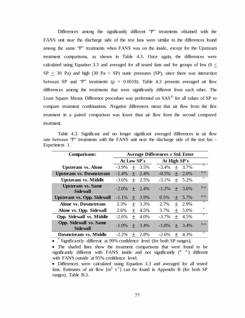
77
Differences among the significantly different “P” treatments obtained with the
FANS unit near the discharge side of the test fans were similar to the differences found
among the same “P” treatments when FANS was on the inside, except for the Upstream
treatment comparisons, as shown in Table 4.3. Once again, the differences were
calculated using Equation 3.3 and averaged for all tested fans and for groups of low (0 <
SP < 30 Pa) and high (30 Pa < SP) static pressures (SP), since there was interaction
between SP and “P” treatments (p = 0.0018). Table 4.3 presents averaged air flow
differences among the treatments that were significantly different from each other. The
Least Square Means Difference procedure was performed on SAS® for all values of SP to
compare treatment combinations. Negative differences mean that air flow from the first
treatment in a paired comparison was lower than air flow from the second compared
treatment.
Table 4.3. Significant and no longer significant averaged differences in air flow
rate between “P” treatments with the FANS unit near the discharge side of the test fan – Experiment 1.
* Significantly different at 99% confidence level (for both SP ranges);
The shaded lines show the treatment comparisons that were found to be significantly different with FANS inside and not significantly (n. o.) different
with FANS outside at 95% confidence level;
Differences were calculated using Equation 3.3 and averaged for all tested
fans. Estimates of air flow [m3 s-1] can be found in Appendix B (for both SP ranges), Table B.3.
Comparisons: Average Differences ± Std. Error
At Low SP`s
At High SP`s
Upstream vs. Alone -3.9% 3.5%
-3.4% 3.7%
*
Upstream vs. Downstream -1.4% 2.4%
-0.5% 2.0%
n.o.
Upstream vs. Middle -3.6% 2.5%
-3.1% 5.2%
*
Upstream vs. Same
Sidewall -2.0% 2.4%
-1.2% 3.6%
n.o.
Upstream vs. Opp. Sidewall -1.1% 3.9%
0.5% 5.7%
n.o.
Alone vs. Downstream 2.3% 3.3%
2.7% 2.9%
*
Alone vs. Opp. Sidewall 2.6% 4.5%
3.7% 5.0%
*
Opp. Sidewall vs. Middle -2.6% 4.0%
-3.7% 4.5%
*
Opp. Sidewall vs. Same
Sidewall -1.0% 3.4%
-1.8% 3.4%
n.o.
Downstream vs. Middle -2.2% 2.8%
-2.6% 4.3%
*

78
Placing the FANS unit outside the barn reduced the number of “P” treatments that
were significantly different from each other and also reduced the magnitude of the
differences between the Upstream and the remaining “P” treatments. The differences
between the Upstream treatment and the other “P” treatments obtained with FANS
outside were approximately 75.6 ± 13.8 % lower than the same differences encountered
with FANS inside. This reduction in the differences between Upstream and remaining
“P” treatments is evidence that the FANS unit causes an air flow penalty in the Upstream
treatment, when placed next to the intake side of the test fan.
Still, there were significant differences up to 3.9 ± 3.5% (Table 4.3) between the
Upstream and Alone treatments when the FANS unit was placed near the discharge side
of each test fan. This difference indicates that there may also be an actual difference in
fan performance between those two treatment configurations. The Upstream treatment
provided the lowest air flow values with FANS inside and outside. Therefore, that
treatment configuration should be avoided for all fan tests, regardless whether the FANS
unit is placed at the intake or at discharge side of the test fan.
The Opposite Sidewall treatment produced results statistically different from the
results of two other “P” treatments (Table 4.3). The Opposite Sidewall treatment
produced air flow results up to 3.7 ± 5.0% lower than the Alone treatment, which could
lead to a substantial error on the estimation of building ventilation. It is suggested that the
Opposite Sidewall configuration should also be avoided during fan tests with FANS.
Based on the results of this Section, it is reasonable to conclude that the FANS
unit frame is responsible for a substantial portion of the air flow penalty observed in the
Upstream treatment configuration. The other differences found among the remaining “P”
treatments may be attributed to an actual change in fan performance, the FANS unit error
and random error, since some differences were found either when the FANS unit was
placed next to the intake or near the discharge sides of the test fans.
Placing the FANS unit on the discharge side of test fans reduces major air flow
penalties. Still, this configuration should be used with as much care as if the FANS unit
was placed next to the intake side of test fan inside barns similar to the one studied in this
experiment (Sub-section 3.1.1).

79
4.1.3 Contour Plots for Results with the FANS Unit Inside and Outside – Experiment 1
Anemometer output data across the FANS section was plotted to illustrate air
speed distribution across the FANS opening area. Contour plots of air velocity across the
FANS unit are presented for the Alone, Middle and Upstream treatments with FANS
placed next to the intake of a test fan. Figure 4.11 through Figure 4.13 show the air
velocity distribution obtained from testing the fan E1_F2, at the same SP (26.5 ± 0.7 Pa)
for the referred treatment configurations. Table 4.4 shows the average air velocities
obtained by each of five anemometers, as illustrated on Figure 4.11 through Figure 4.13.
Figure 4.11. Air velocity across the FANS unit opening – Alone Inside, E1_F2. Dashed lines indicate the positions of Anemometers 1 through 5.
[m s-1]

80
Figure 4.12. Air velocity across the FANS unit opening – Middle Inside, E1_F2. Dashed lines indicate the positions of Anemometers 1 through 5.
Figure 4.13. Air velocity across the FANS unit opening – Upstream Inside, E1_F2. Dashed lines indicate the positions of Anemometers 1 through 5.
[m s-1]
[m s-1]

81
Table 4.4. Average air velocities from Anemometers 1 through 5 for the Alone, Middle and Upstream treatments - Inside.
Average Air Velocity ± Std. Error [m s -1]
Treatment Anemometer
1 Anemometer
2 Anemometer
3 Anemometer
4 Anemometer
5
Alone (Inside)
4.43 ± 0.58 4.36 ± 0.39 4.18 ± 0.48 4.44 ± 0.38 4.56 ± 0.50
Middle (Inside)
4.66 ± 0.65 4.14 ± 0.49 4.19 ± 0.47 4.52 ± 0.36 4.71 ± 0.54
Upstream (Inside)
4.64 ± 0.57 4.17 ± 0.55 4.53 ± 0.54 5.39 ± 0.60 1.76 ± 1.76
Figure 4.11 and Figure 4.13 show that air velocities were nearly symmetric across
the FANS unit section during the Alone and Middle – Inside treatments. Total average air
velocities were approximately 4.4 and 4.5 m s-1, respectively. Figure 4.13 shows a large
asymmetric blue area (low air speeds) near Anemometers 4 and 5 of the FANS unit,
which corresponds to the upstream side of the FANS (right side of contour plot) during
the fan test on the Upstream configuration. The average air speed for the Upstream –
Inside test was approximately 4.1 m s-1. Air velocity on the downstream side (near
Anemometer 1) of the FANS relative to the barn air flow, however, remained similar to
that observed on FANS downstream side during the Alone and Middle - Inside
treatments.
During the Upstream - Inside test, average air velocity through Anemometer 1
(dowstream side of FANS unit relative to the air flow in the barn, Figure 4.13) was
approximately 2.6 times higher than the average air velocity obtained from Anemometer
5 (upstream side of FANS unit relative to the air flow in the barn, blue area, Figure 4.13).
The Alone and Middle (Inside) test results, however, indicated that Anemometer 5
presented average air velocities of approximately 3.0% and 1.0% higher than the air
velocity provided by Anemometer 1, for the respective tests.
Air velocity provided by Anemometer 5 in the Upstream configuration was
substantially lower than the air velocity provided by the same anemometer in the Middle
and Alone configurations (Table 4.4). On the other hand, Anemometer 3 and 4 provided
higher air velocity readings in the Upstream configuration than in the Alone and Middle
configurations, as shown on Table 4.4. The air velocity profiles shown in Figure 4.11 and

82
Figure 4.12 for the Alone and Middle treatments - Inside are similar to the one found by
Sama et al. (2008) shown in Figure 4.14, which was obtained in laboratory fan tests using
a 1.22 m FANS unit.
Figure 4.14. Air velocity across a 1.22 m FANS unit opening, Sama et al. (2008).Vertical
lines represent the anemometer positions.
Figure 4.15 through Figure 4.17 show contour plots of the anemometer air
velocity outputs across the FANS section for the Alone, Middle and Upstream treatments
with FANS placed near the discharge side of the same test fan ( E1_F2) at the same SP
(26.5 ± 0.7 Pa).
Table 4.5 shows average air velocities obtained from the five anemometers for the
same treatments.

83
Figure 4.15. Air velocity across the FANS unit opening – Alone Outside, E1_F2. Dashed lines indicate the positions of Anemometers 1 through 5.
Figure 4.16. Air velocity across the FANS unit opening – Middle Outside, E1_F2.
Dashed lines indicate the positions of Anemometers 1 through 5.
[m s-1]
[m s-1]

84
Figure 4.17. Air velocity across the FANS unit opening – Upstream Outside, E1_F2 Dashed lines indicate the positions of Anemometers 1 through 5.
Table 4.5. Average air velocities from Anemometers 1 through 5 for the Alone, Middle and Upstream treatments - Outside.
Average Air Velocity ± Std. Error [m s -1]
Treatment Anemometer
1 Anemometer
2 Anemometer
3 Anemometer
4 Anemometer
5
Alone (Inside)
2.62 ± 2.52 5.22 ± 1.23 4.12 ± 2.02 5.79 ± 1.91 4.77 ± 2.37
Middle (Inside)
4.60 ± 2.31 5.04 ± 1.34 3.99 ± 2.02 5.67 ± 1.71 5.01 ± 2.12
Upstream (Inside)
2.68 ± 2.21 5.00 ± 1.27 3.93 ± 2.07 5.59 ± 1.76 4.75 ± 1.47
Figure 4.15 through Figure 4.17 show that the Alone, Middle and Upstream –
Outside treatments provided similar air velocity distributions through the FANS unit
section, with average air velocities of 4.5, 4.5 and 4.4 m s-1, respectively. The average air
velocity through the FANS unit obtained in the Alone and Middle treatment were
approximately the same with FANS placed inside and outside the barn. However, the
average air velocity on the Upstream treatment was approximately 7.0% higher when the
FANS unit was placed outside the barn (4.4 m s-1) than inside (4.1 m s-1) the barn.
[m s-1]

85
Therefore, placing the FANS unit near the discharge side of test fans substantially
reduced the differences between the “P” treatments and the Upstream treatment (Figure
4.11 through Figure 4.13), which is evidence that the FANS unit causes an air flow
penalty, when placed next to the intake side of the test fan in the Upstream treatment.

86
4.2 Experiment 2 (E2) – Farms 2, 3 & 4, Operated by Poultry Company 2
Air flow obtained from each treatment was regressed as a second order
polynomial function of static pressure (SP), as described in section 3.6. The intercept,
first and second order parameters of the regressions are provided in Appendix A, Table
A.2. The addition of the quadratic term was significant at 90% confidence level for
approximately 72% of the regression curves. Therefore, the second order polynomial
regression was performed among all fan tests. The overall models of fan performance
were all significant and presented a strong relationship between air flow and static
pressure. Approximately 82% of the curves had a coefficient of determination (R2) of at
least 98% and overall p-value less than 0.0001. The remaining fan curves presented an R2
of at least 95% and overall p-value less than 0.0006.
4.2.1 Fan Tests with the FANS Unit next to the Intake Side of each Test Fan (Inside
Treatment)-Experiment 2
Figure 4.18 through Figure 4.22 show the fan performance curves obtained in
Experiment 2, with FANS placed next to the intake (Inside treatment) of test fans.

87
Figure 4.18. Fan performance curves, FANS unit Inside, E2_F1.
Figure 4.19. Fan performance curves, FANS unit Inside, E2_F2.
0 10 20 30 40 50 604
5
6
7
8
9
10
11
12
Static Pressure [Pa]
Air
Flo
w [
m3 s
-1]
0 10 20 30 40 50 604
5
6
7
8
9
10
11
12
Static Pressure [Pa]
Air
Flo
w [
m3 s
-1]

88
Figure 4.20. Fan performance curves, FANS unit Inside, E2_F3.
Figure 4.21. Fan performance curves, FANS unit Inside, E2_F4.
0 10 20 30 40 50 604
5
6
7
8
9
10
11
12
Static Pressure [Pa]
Air
Flo
w [
m3 s
-1]
0 10 20 30 40 50 604
5
6
7
8
9
10
11
12
Static Pressure [Pa]
Air
Flo
w [
m3 s
-1]

89
Figure 4.22. Fan performance curves, FANS unit Inside, E2_F5.
Figure 4.18 through Figure 4.22 show that the fan performance curves were
generally similar and close together, except for the fan curves produced by the Upstream
treatment, which generated lower air flow values. The “P” (position of operating fans
relative to FANS and test fan) treatments had a significant (p < 0.0001) effect on air flow.
The treatments Alone, Middle, Same Sidewall and Downstream were not significantly (p
> 0.5000) different from each other and presented, in general, the highest fan
performance curves among the five test fans in Experiment 2, when the FANS unit was
placed next to the intake side of the test fan. The Opposite Sidewall provided fan
performance curves right below the highest fan performance curves.
Similar to Experiment 1, the “Upstream” treatment produced the lowest fan
performances for all test fans with FANS positioned on the intake side. All “P”
treatments were significantly (p < 0.0001) different from the Upstream treatment. Also,
the Opposite Sidewall treatment was significantly (p < 0.0100) different from the
remaining “P” treatments. The difference in air flow between Opposite Wall fan curves
0 10 20 30 40 50 604
5
6
7
8
9
10
11
12
Static Pressure [Pa]
Air
Flo
w [
m3 s
-1]
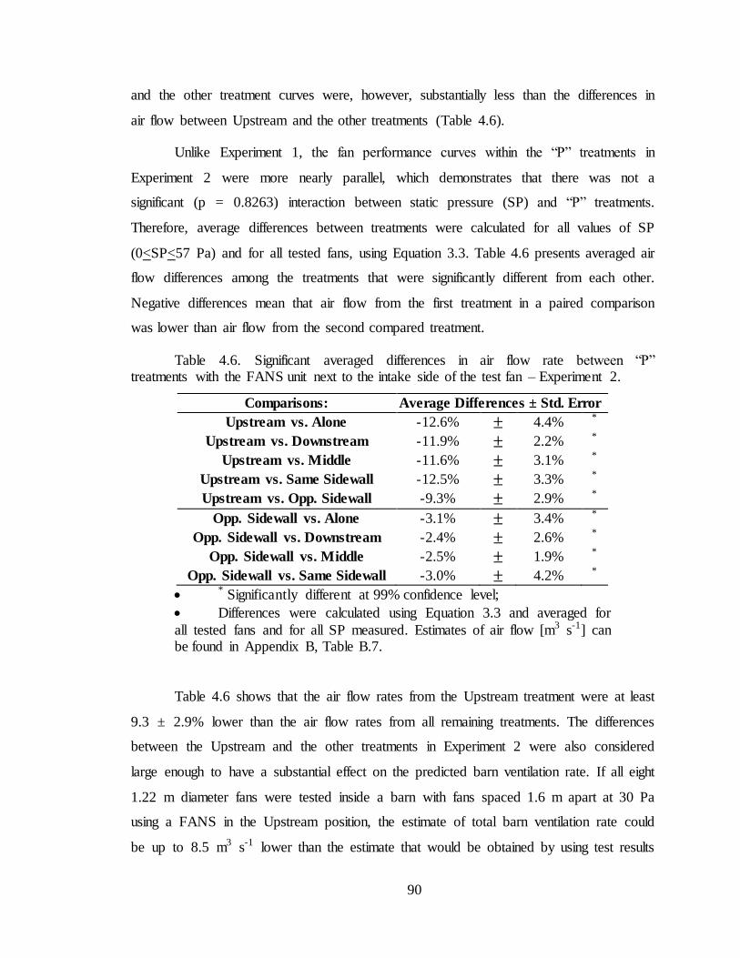
90
and the other treatment curves were, however, substantially less than the differences in
air flow between Upstream and the other treatments (Table 4.6).
Unlike Experiment 1, the fan performance curves within the “P” treatments in
Experiment 2 were more nearly parallel, which demonstrates that there was not a
significant (p = 0.8263) interaction between static pressure (SP) and “P” treatments.
Therefore, average differences between treatments were calculated for all values of SP
(0<SP<57 Pa) and for all tested fans, using Equation 3.3. Table 4.6 presents averaged air
flow differences among the treatments that were significantly different from each other.
Negative differences mean that air flow from the first treatment in a paired comparison
was lower than air flow from the second compared treatment.
Table 4.6. Significant averaged differences in air flow rate between “P” treatments with the FANS unit next to the intake side of the test fan – Experiment 2.
Comparisons: Average Differences ± Std. Error
Upstream vs. Alone -12.6% 4.4% *
Upstream vs. Downstream -11.9% 2.2% *
Upstream vs. Middle -11.6% 3.1% *
Upstream vs. Same Sidewall -12.5% 3.3% *
Upstream vs. Opp. Sidewall -9.3% 2.9% *
Opp. Sidewall vs. Alone -3.1% 3.4% *
Opp. Sidewall vs. Downstream -2.4% 2.6% *
Opp. Sidewall vs. Middle -2.5% 1.9% *
Opp. Sidewall vs. Same Sidewall -3.0% 4.2% *
* Significantly different at 99% confidence level;
Differences were calculated using Equation 3.3 and averaged for
all tested fans and for all SP measured. Estimates of air flow [m3 s-1] can be found in Appendix B, Table B.7.
Table 4.6 shows that the air flow rates from the Upstream treatment were at least
9.3 ± 2.9% lower than the air flow rates from all remaining treatments. The differences
between the Upstream and the other treatments in Experiment 2 were also considered
large enough to have a substantial effect on the predicted barn ventilation rate. If all eight
1.22 m diameter fans were tested inside a barn with fans spaced 1.6 m apart at 30 Pa
using a FANS in the Upstream position, the estimate of total barn ventilation rate could
be up to 8.5 m3 s-1 lower than the estimate that would be obtained by using test results

91
from the Alone or Middle treatments. An 8.5 m3 s-1 (18,010 cfm) difference in air flow
rate is roughly equivalent to the amount of air that two new 0.91 m (36 in) diameter fans
move at the same static pressure.
Once again, substantial differences between the Upstream and the remaining “P”
treatment results indicate that either the test fans were operating at lower air flow
capacities or the FANS unit was possibly causing an air flow penalty when the Upstream
configuration of operating fans was used inside the barns of Farm 2, 3 and 4. The
Upstream treatment configuration should, therefore, be avoided when testing fans using
the FANS unit inside barns similar to the ones studied in Farm 2, 3 and 4 (Sub-sections
3.1.2, 3.1.3 and 3.1.4).
Average differences between the Opposite Sidewall and the remaining treatments
were approximately 3.1 ± 3.4% or less. Still, those differences could be large enough to
cause a substantial total air flow error in the building ventilation rate estimation.
Therefore, it is recommended that the Opposite sidewall treatment configuration should
also be avoided when testing fans using the FANS unit inside barns similar to the ones
studied in this work (Sub-sections 3.1.2, 3.1.3 and 3.1.4).
Fans that were tested in this study were located on the sidewalls of the exhaust
end of the barns. Therefore, the air has to make a 90o turn to pass through the FANS unit
and test fan (see Figure 3.32 through Figure 3.37). It is reasonable to assume that the
FANS unit frame can actually work as an obstacle in the air path from the curtain inlets
through the exhaust fans. Placing the FANS unit near the discharge side of the test fan
(Outside treatment) would remove any potential obstruction from the fan intake and
allow air to flow freely into the fan. Similar to Experiment 1, fan tests were performed
with the FANS unit placed near the discharge side of test fans (Figure 3.43 through
Figure 3.48) and an analysis was performed to determine if the differences were caused
by penalties related to the FANS unit structure or by a real change in the actual fan
performance (Sub-section 4.1.2).

92
4.2.2 Fan Tests with the FANS Unit near the Discharge Side of each Test Fan (Outside
Treatment) – Experiment 2.
The FANS unit was placed outside of the barn, near the discharge side of test fans
as described in Sub-section 3.3.2 and all “P” treatments were run again. This FANS unit
placement allowed air to go straight through the FANS unit after it had passed through
the test fan. Therefore, it was expected that the differences between the “P” treatments
would be reduced when fan tests were performed with FANS outside of the barn. Figure
4.23 through Figure 4.27 show fan performance curves obtained in Experiment 2, with
FANS placed near the discharge side (Outside treatment) of test fans.
Figure 4.23. Fan performance curves, FANS unit Outside, E2_F1.
0 10 20 30 40 50 604
5
6
7
8
9
10
11
12
Static Pressure [Pa]
Air
Flo
w [
m3 s
-1]

93
Figure 4.24. Fan performance curves, FANS unit Outside, E2_F2.
Figure 4.25. Fan performance curves, FANS unit Outside, E2_F3.
0 10 20 30 40 50 604
5
6
7
8
9
10
11
12
Static Pressure [Pa]
Air
Flo
w [
m3 s
-1]
0 10 20 30 40 50 604
5
6
7
8
9
10
11
12
Static Pressure [Pa]
Air
Flo
w [
m3 s
-1]

94
Figure 4.26. Fan performance curves, FANS unit Outside, E2_F4.
Figure 4.27. Fan performance curves, FANS unit Outside, E2_F5.
0 10 20 30 40 50 604
5
6
7
8
9
10
11
12
Static Pressure [Pa]
Air
Flo
w [
m3 s
-1]
0 10 20 30 40 50 604
5
6
7
8
9
10
11
12
Static Pressure [Pa]
Air
Flo
w [
m3 s
-1]

95
Figure 4.23 through Figure 4.27 show that the fan performance curves were closer
together for all “P” treatments with the FANS unit outside than with the FANS unit
inside the barn (Figure 4.18 through Figure 4.22). Performance curves obtained from the
Upstream treatment were generally closer to performance curves from the remaining
treatments when the FANS unit was placed near the discharge side the test fans than
when the FANS unit was placed next to the intake side of test fans. The change in air
flow results caused by placing the FANS unit outside the barn demonstrates that there
was interaction between the “P” and the “S” treatments (p<0.0001).
Statistical tests showed that the “S” treatments (FANS inside vs. FANS outside)
had no significant (p = 0.0631) effect on air flow measurements. The “P” treatments
obtained with the FANS unit next the intake side of the test fan (Inside treatment) were
not significantly different (p < 0.05) from the same “P” treatments obtained with the
FANS unit near the discharge side of the test fan, with exception of the Upstream and
Opposite Sidewall treatments (Table 4.7). Therefore the Alone, Downstream, Middle and
Same Sidewall treatments presented similar results to the ones found by Li et al. (2009),
who did not find significant differences between fan test results obtained by placing the
FANS unit next to the intake side of the test fan versus placing the FANS unit near the
discharge side of the test fan.
Table 4.7. Comparison of FANS Inside versus FANS Outside within the same “P” treatment – Experiment 2. Average differences in air flow calculated for all tested fans
and SP.
Comparison Average Differences ± Std. Error
Alone IN vs. OUT 1.56% ± 2.47% n
Upstream IN vs. OUT -10.08% ± 5.81% **
Downstream IN vs. OUT -0.23% ± 3.36% n
Middle IN vs. OUT -0.44% ± 5.66% n
Same Sidewall IN vs. OUT 1.68% ± 4.00% n
Opposite Sidewall
IN vs. OUT -2.31% ± 5.67% **
n Not significantly different at 95% confidence level.
** Shaded lines show treatments that provided significantly
different results between FANS placed on the intake of test fan or on the discharge of the test fan at 95% confidence level;

96
The “P” treatments found to be significantly different from other “P” treatments
when the FANS unit was placed next to the intake of the test fan were compared again
with the FANS unit placed near the discharge side of the test fan. When the FANS unit
was placed outside the barn, the Upstream treatment was no longer significantly different
from all other treatments, as was found when the FANS was placed on the inside of the
barn. The Upstream treatment with the FANS near the discharge side of the test fan
provided fan performance curves significantly (p < 0.05) different from the curves
obtained from the Downstream and Middle treatments. Also, with FANS placed near the
discharge side of the test fans, the Opposite Sidewall treatment was no longer
significantly different (p<0.05) from the remaining treatments, as was found when the
FANS was placed next to the intake of the test fans.
This change among the differences between the “P” treatments indicates that
placing the FANS unit near the discharge side of the test fans contributed to reduce the
number of significantly different “P” treatments. When the FANS unit was placed next to
the intake of the test fan, 11of the 15 possible comparisons among the “P” treatments
were found to be significantly different. However, when the FANS unit was placed near
the discharge of the test fan, only four of the 15 possible comparisons were found to be
significantly different.
Although placing the FANS unit near the discharge side of the test fans caused
some treatments not to be significantly (p < 0.05) different from each other, the Middle
treatment differed from Alone, Upstream and Same Sidewall treatments, when the FANS
unit was placed near the discharge side of the test fan. These differences, however, were
less than 2% of the fan air flow rate (Table 4.8) and are unlikely to be of any practical
importance.
The differences among the “P” treatments with the FANS unit placed on the
outside of the barns were calculated among the treatments that were significantly
different from each other when the FANS unit was placed both on the inside and outside
of the barn. The static pressure (SP) did not interact with treatments at 95% confidence
level. Differences were calculated using Equation 3.3 for all static pressure values and for
all tested fans.

97
Table 4.8. Significant and no longer significant averaged differences in air flow rate between “P” treatments with the FANS unit near the discharge side of the test fan –
Experiment 2.
Comparisons: Average Differences ± Std. Error
Upstream vs. Alone -0.8% 3.5% n.o.
Upstream vs. Downstream -2.0% 3.9% **
Upstream vs. Middle -2.2% 4.6% *
Upstream vs. Same Sidewall -0.5% 3.0% n.o.
Upstream vs. Opp. Sidewall -1.5% 1.9% n.o.
Opp. Sidewall vs. Alone 0.7% 3.7% n.o.
Opp. Sidewall vs. Downstream -0.5% 4.3% n.o.
Opp. Sidewall vs. Middle -0.7% 4.8% n.o.
Opp. Sidewall vs. Same Sidewall 1.0% 2.8% n.o.
Middle vs. Alone 1.3% 0.04% **
Middle vs. Same Sidewall 0.1% 0.03% *
The shaded lines show the treatment comparisons that were found to be significantly different with FANS inside and not significantly (n.o.) different with FANS outside at 95% confidence
level;
* Significantly different at 99% confidence level; ** Significantly
different at 95% confidence level;
Differences were calculated using Equation 3.3 and averaged for
all tested fans. Estimates of air flow [m3 s-1] can be found in Appendix B (for both SP ranges), Table B.7.
Placing the FANS unit outside the barn reduced the number of “P” treatments
significantly different from each other and reduced the magnitude of differences between
the Upstream and the remaining “P” treatments. The differences between the Upstream
treatment and the other “P” treatments obtained with FANS outside were approximately
87.5 ± 6.8 % lower than the same differences encountered with the FANS inside, which
is evidence that the FANS unit causes an air flow penalty in the Upstream treatment,
when placed next to the intake side of a test fan.
Still, there were significant differences up to 2.2 ± 4.6% (Table 4.3) between the
Upstream and Middle treatments when the FANS unit was placed near the discharge side
of each test fan. This result indicates that there may be also an actual difference in fan
performance between these treatment configurations. Also, the difference standard error
is relatively high compared to the average difference between these two treatments

98
Therefore, this treatment configuration should be avoided either when the FANS unit is
placed next to the intake or near the discharge sides of the test fan.
Unlike when the FANS unit was placed next to the intake side of the test fan, the
Opposite Sidewall treatment did not produce air flow results statistically different from
results from the other “P” treatments (Table 4.3) with the FANS unit placed near the
discharge side of the test fans. The Opposite Sidewall configuration should be avoided
during fan tests with the FANS unit placed next to the intake of the test fan. However,
this treatment configuration may be used to test fans with the FANS unit near the
discharge side of the test fan, inside barns similar to the ones studied in this experiment,
with fans spaced 1.6 m apart (Sub-sections 3.1.2, 3.1.3, and 3.1.4).
Based on the results of this Section, it is reasonable to conclude that the FANS
unit frame is responsible for a substantial portion of the air flow penalty observed in the
Upstream and Opposite Sidewall treatment configurations. Differences between other “P”
treatments may be attributed to real variations in fan performance, FANS unit error and
random error, since some similar differences were found when the FANS unit was placed
on both the intake and discharge sides of the test fans. Placing the FANS unit on the
discharge side of the test fan minimizes the potential air flow penalties without adversely
affecting fan performance results. Thus it appears to be a good configuration option to
test fans in-situ.
4.2.3 Contour Plots for Results with the FANS Unit Inside and Outside – Experiment 2
Anemometer output data across the FANS section was plotted to illustrate the air
speed distribution across the FANS opening area. Contour plots of air velocity through
the FANS unit are presented for the Alone, Middle and Upstream treatments for the
FANS placed next to the intake side of a test fan. Figure 4.28 through Figure 4.30 show
the air velocity distribution obtained from testing the fan E2_F3 at the static pressure (SP)
30.7 ± 1.9 Pa. Table 4.9 shows the average air velocities obtained by each of five
anemometers for the referred treatments.

99
Figure 4.28. Air velocity across the FANS unit opening – Alone Inside, E2_F3. Dashed lines indicate the positions of Anemometers 1 through 5.
[m s-1]

100
Figure 4.29. Air velocity across the FANS unit opening – Middle Inside, E2_F3. Dashed
lines indicate the positions of Anemometers 1 through 5.
Figure 4.30. Air velocity across the FANS unit opening – Upstream Inside, E2_F3. Dashed lines indicate the positions of Anemometers 1 through 5.
[m s-1]
[m s-1]

101
Table 4.9. Average air velocities from Anemometers 1 through 5 for the Alone, Middle and Upstream treatments (Inside).
Average Air Velocity ± Std. Error [m s -1]
Treatment Anemometer
1 Anemometer
2 Anemometer
3 Anemometer
4 Anemometer
5
Alone (Inside)
5.53 ± 0.72 5.15 ± 0.54 4.97 ± 0.61 5.11 ± 0.48 3.88 ± 0.97
Middle (Inside)
5.77 ± 0.79 5.15 ± 0.60 5.09 ± 0.55 4.96 ± 0.46 3.91 ± 1.06
Upstream (Inside)
5.46 ± 0.58 5.10 ± 0.55 5.12 ± 0.68 5.39 ± 0.60 1.33 ± 1.69
Figure 4.28 and Figure 4.29 show that there were small areas of reduced air
velocity on the upstream side of the FANS unit (right side of contour plots) in both Alone
and Middle - Inside treatments. Anemometer 1 (downstream side of FANS unit, relative
to the air flow in the barn) produced average air velocities 42.6% and 47.5% higher than
Anemometer 5 (upstream side of FANS unit relative to the air flow in the barn), for the
Alone and Middle - Inside treatments, respectively. The average air velocities obtained in
the Alone and Middle - Inside treatments were approximately 4.9 and 5.0 m s-1,
respectively. Similar patterns of air velocity distribution were found for the Alone
treatment Inside for Fans 1, 2 and 4 as well.
Contour plots shown in Figure 4.28 and in Figure 4.29 differ from Figure 4.11
and Figure 4.12 obtained in Experiment 1 since the Alone and Middle - Inside treatments
in Experiment 1 (E 1) provided air velocities more uniformly distributed across the
FANS opening. The difference in air velocity profiles through the FANS opening could
be an indication that air velocity through the FANS unit is related to air flow penalties
obtained with the FANS unit, since this difference in air velocity profile was observed for
four of the five tested fans in this experiment. Therefore, a further analysis of air velocity
differences between FANS anemometers was performed to verify if these differences
were related to average barn air speed, described in Section 4.3.
Figure 4.30 shows a larger asymmetric blue area (low air speeds) on the upstream
side of the FANS unit relative to the barn air flow (right side of contour plot). The
average air speed for the Upstream – Inside test was approximately 4.5 m s-1.
Anemometer 1 provided an average air velocity approximately 4.1 times higher than the

102
air speed obtained from Anemometer 5. Air velocity provided by Anemometer 5 in the
Upstream configuration was substantially lower than the air velocity provided by the
same anemometer in the Middle and Alone configurations (Table 4.5). On the other hand,
Anemometer 3 and 4 provided higher air velocity readings in the Upstream configuration
than in the Alone and Middle configurations, as shown on Table 4.5.
Figure 4.31 through Figure 4.33 show contour plots of the anemometer air
velocities output across the FANS section for the Alone, Middle and Upstream treatments
with FANS placed near the discharge side of the same test fan , E2_F3, at the same SP
(30.7 ± 1.9 Pa). Table 4.10 shows the average air velocities obtained by each of five
anemometers for the referred treatments.
Figure 4.31. Air velocity across the FANS unit opening – Alone Outside, E2_F3. Dashed
lines indicate the positions of Anemometers 1 through 5.
[m s-1]

103
Figure 4.32. Air velocity across the FANS unit opening – Middle Outside, E2_F3.
Dashed lines indicate the positions of Anemometers 1 through 5.
Figure 4.33. Air velocity across the FANS unit opening – Upstream Outside, E2_F3.
Dashed lines indicate the positions of Anemometers 1 through 5.
[m s-1]
[m s-1]
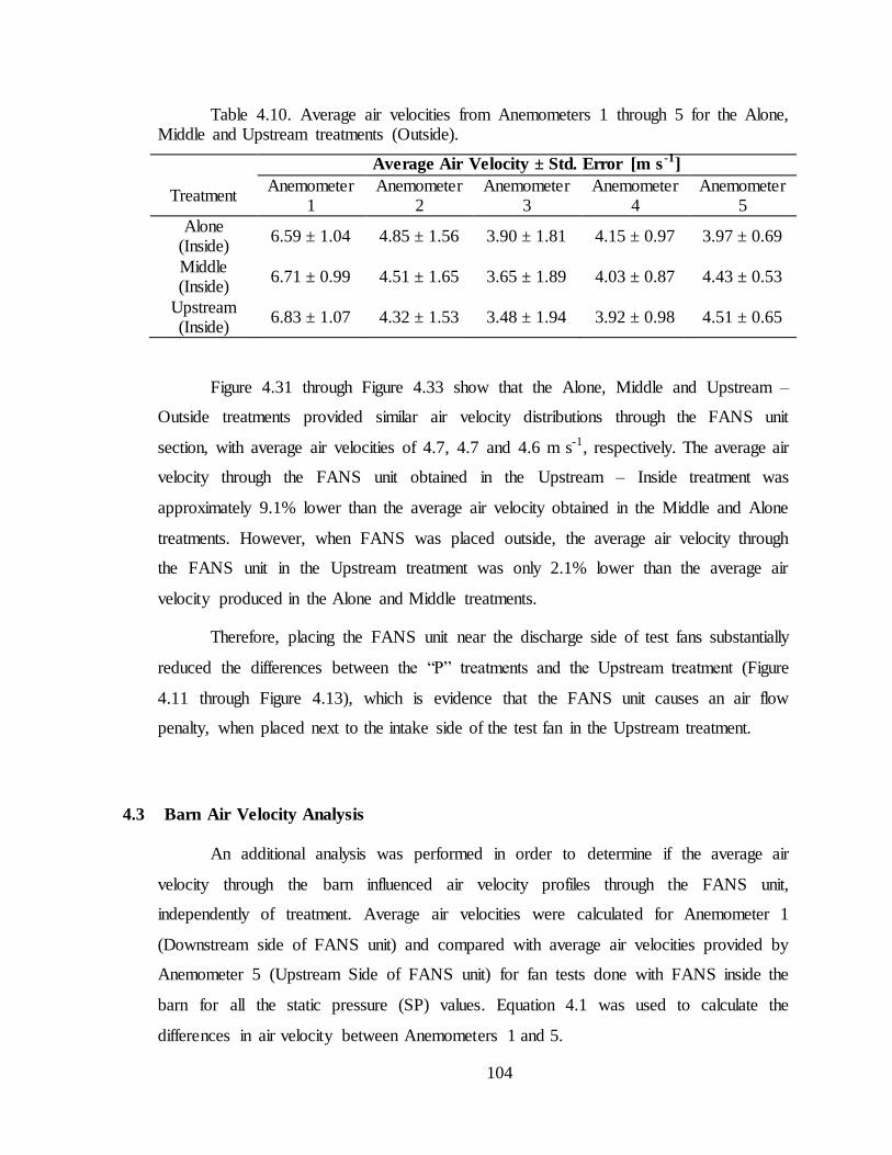
104
Table 4.10. Average air velocities from Anemometers 1 through 5 for the Alone, Middle and Upstream treatments (Outside).
Average Air Velocity ± Std. Error [m s -1]
Treatment Anemometer
1 Anemometer
2 Anemometer
3 Anemometer
4 Anemometer
5
Alone (Inside)
6.59 ± 1.04 4.85 ± 1.56 3.90 ± 1.81 4.15 ± 0.97 3.97 ± 0.69
Middle (Inside)
6.71 ± 0.99 4.51 ± 1.65 3.65 ± 1.89 4.03 ± 0.87 4.43 ± 0.53
Upstream (Inside)
6.83 ± 1.07 4.32 ± 1.53 3.48 ± 1.94 3.92 ± 0.98 4.51 ± 0.65
Figure 4.31 through Figure 4.33 show that the Alone, Middle and Upstream –
Outside treatments provided similar air velocity distributions through the FANS unit
section, with average air velocities of 4.7, 4.7 and 4.6 m s-1, respectively. The average air
velocity through the FANS unit obtained in the Upstream – Inside treatment was
approximately 9.1% lower than the average air velocity obtained in the Middle and Alone
treatments. However, when FANS was placed outside, the average air velocity through
the FANS unit in the Upstream treatment was only 2.1% lower than the average air
velocity produced in the Alone and Middle treatments.
Therefore, placing the FANS unit near the discharge side of test fans substantially
reduced the differences between the “P” treatments and the Upstream treatment (Figure
4.11 through Figure 4.13), which is evidence that the FANS unit causes an air flow
penalty, when placed next to the intake side of the test fan in the Upstream treatment.
4.3 Barn Air Velocity Analysis
An additional analysis was performed in order to determine if the average air
velocity through the barn influenced air velocity profiles through the FANS unit,
independently of treatment. Average air velocities were calculated for Anemometer 1
(Downstream side of FANS unit) and compared with average air velocities provided by
Anemometer 5 (Upstream Side of FANS unit) for fan tests done with FANS inside the
barn for all the static pressure (SP) values. Equation 4.1 was used to calculate the
differences in air velocity between Anemometers 1 and 5.

105
Differences_An. (%) = (ANEM1 – ANEM5)*100/ ANEM5 Equation 4.1
Where,
Differences_An. = Differences [%] between the average air velocities provided
by Anemometers 1 and 5;
ANEM1 = Average air velocity [m s-1] provided by the Anemometer 1;
ANEM5 = Average air velocity [m s-1] provided by the Anemometer 5;
An analysis of variance (Equation 4.2) was performed in order to determine if
the differences between Anemometers 1 and 5 could be described as a function of “P”
treatments and barn air speed (BS). A completely randomized design with a one way
treatment classification approach was used in this analysis. Data of BS at the Alone
treatment was not used in the analysis, once the equipment used to measure air velocity
through the barn (Figure 3.26) was not accurate enough to measure the low air speeds
achieved in the barn during this treatment.
Differences_An(ij)k = µ+Pi+BSj+(P * BS )ij+E(ij)k Equation 4. 2
Where,
µ = overall mean considered common to all observations [%];
Pi = fixed effect on the i-th level of treatment “P”, i = {1,2,3,4,5}, FANS position
relative to operating fans;
BSk = continuous variable, air velocity through the barn [m s-1] to the level of the
k-th experimental unit;
E(ij)k = random component, which explains the random variation or experimental
error to the k-th experimental unit;
Differences_An.(ijl)k = air flow difference between anemometers from the effect
of the i-th and j-th treatment effects, to the level of the k-th experimental unit.

106
PROC GLM was used on SAS® (9.2, SAS Institute Inc., 2002-2008 Cary, NC,
U.S.A) to test the model of analysis of variance described in Equation 4.2. Fans were not
blocked, once they were rejected as significant source of variability among
Differences_An.
The statistical results showed that the overall model of analysis of variance was
significant (p < 0.0001) for Experiments 1 and 2 (Appendix C). Barn air speed
significantly (p = 0.0020) influenced the differences between Anemometers 1 and 5 in
Experiment 2. However, only 2.4% (R2) of the variation in the differences between
anemometers were explained by the variation in barn airspeed. Barn air speed did not
significantly (p=0.5290) affect the differences between Anemometers 1 and 5 in
Experiment 1. The average air velocity through the barns during the fan tests were 1.3 ±
0.3 m s-1 and 1.5 ± 0.4 m s-1 for Experiments 1 and 2 respectively.
These results reject the hypothesis that the average air velocity through the barn
influence air velocity profiles through the FANS unit. Still, it is suggested that a further
study is performed in laboratory to evaluate the relationship between air velocity and
possible air flow penalties obtained with the FANS unit.

107
CHAPTER 5
SUMMARY AND CONCLUSIONS
5.1 Experiment 1 (E 1) – Farm 1, Operated by Poultry Company 1
Fan performance curves were obtained by regressing air flow as a quadratic
function of static pressure (SP), using PRO REG on SAS® (9.2, SAS Institute Inc., 2002-
2008 Cary, NC, U.S.A). All the fan performance curves obtained in this study were
significant. Also, at least 95% of the variation in air flow was explained by the variation
in static pressure.
All the “P” treatments (position of operating fans relative to FANS and test fan)
significantly affected FANS test results. The “S” treatments (FANS inside/outside the
barn) also significantly affected FANS test results. However, for the same “P” treatment,
with exception of the Upstream treatment, fan test results obtained with the FANS unit
placed next to the intake of the test fan (Inside treatment) were not significantly different
from fan test results obtained with the FANS unit placed near the discharge side of the
test fan (Outside treatment). These results agree with those found by Li et al. (2009).
Therefore, a FANS unit can be used on the discharge side of the test fan to measure
performance of fans located in barns similar to those of Farm 1.
The Upstream treatment produced air flow rates as much as 10.9 ± 2.0% lower
than the air flow values obtained from remaining “P” treatments. The Opposite Sidewall
treatment produced air flow results up to 3.5 ± 2.5% lower than the Middle treatment.
Therefore care should be taken during fan tests in-situ to select fans to operate during fan
tests with the FANS unit, so that the test results are as close as possible to the real flow
performance of the test fan.
Placing the FANS unit near the discharge side of test fans provided different
results within the “P” treatments. Some of the “P” treatments that were considered
significantly different from each other based on results with FANS inside the barn were
not found to be significantly different when the FANS unit was placed near the discharge
side of the test fans (Table 4.3). Also, the differences between Upstream and the other

108
“P” treatments were reduced in approximately 75.6 ± 13.8 %. This reduction leaded to
the conclusion that part of the air flow reduction in the Upstream treatment is attributed
to the FANS unit frame, possibly acting as an obstruction to the air as it moves toward
the fan intake.
The other differences found among the “P” treatments may be attributed to an
actual change in fan performance, FANS unit error and random error, since some
differences were found either when the FANS unit was placed next to the intake or near
the discharge sides of the test fans. Placing the FANS unit on the discharge side of the
test fan minimizes the air flow penalties, thus it is a good configuration option to test fans
in-situ.
It was concluded that the Upstream and Opposite Sidewall treatment
configurations should be avoided during fan tests in-situ with the FANS unit placed both
on the intake and on the discharge side of test fans located inside barns similar to the ones
studied in Experiment 1 of this work (with fans placed immediately next to each other).
The results of Experiment 1and 2 were used to elaborate a procedure for using the
FANS unit for in-situ testing of ventilation fans, as described in Section 5.4.
Recommendations were provided regarding number of runs and, especially, regarding
ways of changing static pressure in the barn during fan tests with FANS.
5.2 Experiment 2 (E 2) – Farms 2, 3 and 4, Operated by Poultry Company 2
Fan performance curves were obtained by regressing air flow as a quadratic
function of static pressure, using PROC REG in SAS® (9.2, SAS Institute Inc., 2002-
2008 Cary, NC, U.S.A). All fan performance curves presented significant relationship
between air flow and static pressure. Also, at least 95% of the variation in air flow was
explained by the variation in static pressure.
All “P” (position of operating fans relative to FANS and test fan) treatments had a
significant effect on air flow. On the other hand, the “S” treatments (FANS inside/outside
the barn) did not present significant effect on air flow. Similar to Experiment 1, fan tests
results obtained with FANS unit placed next to the intake of the test fan (Inside

109
treatment), within the same “P” treatment with exception of the Upstream and Opposite
Sidewall treatments, were not significantly different from fan test results obtained with
FANS placed near the discharge side of the test fan (Outside treatment, P – value > 0.07),
which agrees with findings by Li et al. (2009). Therefore, the FANS unit can be used on
the discharge side of the test fan to measure fan performance of fans located in barns
similar to the ones of Farms 2, 3 and 4.
Static pressure did not interact with “P” treatments. The absence of this
interaction may be seen graphically by observing that the fan performance curves were
nearly parallel among all the treatments.
Fan test results from the Upstream treatment were as much as 12.6 ± 4.4% lower
than the remaining “P” treatments. Also, the Opposite Sidewall produced air flow results
up to 3.1 ± 3.4% lower than results obtained from the remaining “P” treatments.
Therefore, these two treatments should be avoided when testing fans in-situ using the
FANS unit inside barns similar to the ones studied in this experiment (Sub-sections 3.1.2,
3.1.3 and 3.1.4).
Placing the FANS unit near the discharge side of the test fans provided different
responses of the “P” treatments. Some “P” treatments that were considered significantly
different from each other based on results with the FANS unit inside the barn were not
found to be significantly different when the FANS unit was placed near the discharge
side of the test fans (Table 4.8). The Opposite Sidewall treatment configuration may be
used in fan tests with FANS near the discharge of test fans. Also, differences between
Upstream and other “P” treatments were reduced by approximately 87.5 ± 6.8 %. This
reduction in air flow differences led to the conclusion that part of the air flow reduction in
the Upstream treatment is attributed to the FANS unit frame, possibly acting as an
obstruction to the air as it moves toward the fan intake.
Other differences found among the “P” treatments may be attributed to an actual
change in fan performance, FANS unit error and random error, since some differences
were found either when the FANS unit was placed next to the intake or near the discharge
sides of the test fans.

110
The results of Experiment 1 and 2 were used to elaborate a procedure for using
the FANS unit for in-situ testing of ventilation fans, as described in Section 5.4.
Recommendations were provided regarding number of runs and, especially, regarding
ways of changing static pressure in the barn during fan tests with FANS.
5.3 General Findings
The fan performance setups (Sub-sections 3.3.1 and 3.3.2) and the fan test
procedure with the FANS unit used in this study (Sub Section 3.3.4) were adequate and
provided good models to predict air flow rate based on static pressure (SP) values. The
second order polynomial fan performance curves were all significant at 95% confidence
level and presented strong relationships between air flow and SP (R2 > 95%). Therefore,
either the setup or the procedure used in this work are recommended for testing fans in-
situ with the FANS unit.
The FANS unit position relative to the operating fans in the barns (“P”
treatments) significantly affected air flow results for both types of poultry barns evaluated
in this study, described in Section 3.1. The Upstream treatment was as much as 12.6 ±
4.4% lower than the remaining “P” treatments. The Opposite Sidewall treatment was as
much as 3.1 ± 3.4% lower than the remaining treatments in Experiment 2. Therefore, the
Upstream and Opposite Sidewall treatment configuration should be avoided during fan
tests in-situ using the FANS unit inside barns similar to the ones studied in this work.
Placing the FANS unit on the outside of the barn, near the fan discharge cone
(Outside treatment), reduced the differences between the Upstream and the remaining “P”
treatments in at least 75.6 ± 13.8 %. The inside and outside placement of the FANS unit
(“S” treatments) did not influence air flow results for the same “P” treatment, with
exception of the Upstream treatment in Experiment 1and the Upstream and Opposite
Sidewall treatments in Experiment 2. Therefore, it was established in this study that the
position of the FANS unit relative to operating fans in the Upstream and Opposite
Sidewall treatment configurations in the barns affects fan performances results, owing

111
mainly to the FANS unit frame, change in the fan actual performance, FANS unit error
and random error.
The Upstream and Opposite sidewall treatment configuration should also be
avoided when testing fans in-situ with the FANS unit placed near the discharge side of
fans located inside barns similar to those of Experiment 1 (Sub-section 3.1.1). However,
when testing fans in-situ with the FANS unit placed near the discharge side of fans
located in barns similar to the ones studied in Experiment 2 (Sub-sections 3.1.2, 3.1.3 and
3.1.4), all the treatment configurations may be used, with exception of the Upstream
configuration.
Results from this study showed the need of a standardized method for using the
FANS unit to test fans in-situ, minimizing possible penalties related to the FANS unit. A
procedure for testing fans with the FANS unit was proposed based on the results of this
work and was presented in Section 5.4. Changing the SP in the barn, as well as the FANS
unit setup and number of test runs were considered when developing the procedure for
using the FANS unit in-situ.
5.4 Procedure for Using the FANS Unit in-situ
Field conditions for testing fans are different from laboratory conditions, therefore
it is beneficial to make a few recommendations for using the FANS unit in-situ. These
recommendations are listed below and are based on the results of this study.
1. Properly Seal the FANS unit to the intake/discharge of the test fan: All fan
performance curves obtained in this study presented strong and significant relationships
between air flow and static pressure. Therefore, before using the FANS unit to perform
fan testing, it is recommended that the FANS unit be sealed to the intake or discharge of
the test fan, since this practice provided good fan test results in this study. Further, it is
recommended that the FANS unit opening area is not smaller than the opening area of the
fan discharge cones;
2. Static Pressures/Number of Runs: It is recommended that a few values of
static pressure (SP) are chosen to build fan performance curves that represent the fan

112
operation in-situ. Eight values of SP provided strong and significant fan performance
curves in this study. However, Lopes et al. (2010) also obtained good fan performance
results with readings at five different SP. Therefore, the number of SP readings can be
flexible depending on the SP range needed to be covered. It is not recommended to use
SP values above 60Pa (≡ 0.24 in.H2O) inside poultry barns, since high SP could possibly
damage surfaces such as the ceiling. Also, the differential pressure transducer used in the
FANS unit has an operational range of 0 – 62 Pa (0 - 0.25 in.H2O, Figure 3.19).
3. Changing the SP in the Barn:
Changing the SP in the building is necessary to build performance curves of
ventilation fans. Therefore, a few recommendations for changing SP during fan tests with
the FANS unit are presented in this Sub-section.
Fan tests with FANS next to the intake side of test fan (Inside the barn):
a) Preference should be given for changing the SP by closing the tunnel
curtains and doors before activating additional fans;
b) If closing the barn does not provide sufficiently high SP values, other fans
should be activated, beginning with fans located in the other end of the
barn (the greatest distance from the test fan);
c) If more operating fans are needed to raise the SP, activate fans upstream of
the test fan, making the FANS unit and test fan in the downstream position
relative to the tunnel air flow (Figure 3.33). Activate as many fans as
possible upstream from the FANS unit and test fan, starting with fans on
the same sidewall as FANS and then turning on the fans upstream to the
FANS on the opposite sidewall from the FANS unit;
d) If the upstream operating fans are not enough to raise the SP, keep the
upstream fans operating and activate fans downstream from the FANS,
making the test fan and FANS unit to be in the Middle position (Figure
3.34). Activate as many fans as possible downstream from the test fan and
FANS unit, starting with the fans on the same sidewall as the FANS and

113
test fan. Then, activate fans downstream from the FANS unit on the
opposite sidewall from the FANS unit and test fan, if necessary;
e) If there are no fans downstream from the test fan (test fan in the exhaust
end corner, for instance), activate fans on the same sidewall as the test fan
and FANS unit. If higher SP is needed inside the barn, keep the fans
operating on the same sidewall as the FANS unit and turn on fans on the
opposite sidewall from the FANS unit, which will put the FANS unit in
the Downstream configuration;
f) If there are no fans upstream from the test fan (last test fan from the
exhaust end, for instance), the fan should be tested alone (Figure 3.35). In
this configuration, all other tunnel fans would be downstream to the FANS
unit which would replicate the Upstream treatment (Figure 3.32). This
research has shown this condition provided the highest air flow differences
from the other treatments in this study. If it is not possible to reach the SP
needed for the fan test, turn on fans located in the other end of the barn
(the greatest distance from the test fan). Activating additional fans in this
situation is not recommended. If higher SP values are really needed, place
the FANS unit near the discharge side of the test fan and run tests turning
on the least number of tunnel fans as possible. However, this configuration
should be avoided, once it could cause air flow penalties up to 3.9 ± 3.5%.
Fan tests with FANS near the discharge side of test fan:
g) Placing the FANS unit near the discharge side of the fan is a good option
if the conditions of topography and vegetation allow placement outside of
the barn. Still, all the steps for testing fans with the FANS unit next to the
intake side of the test fans should be followed even when the FANS unit is
near the discharge side of the test fan. Fans downstream of the FANS unit
should be avoided to raise the SP in the barn. This would set the FANS
unit and test fan in the Upstream position (Figure 3.43), which provided
the highest differences in air flow compared to the other treatments in this
study. The Opposite Sidewall configuration should also be avoided

114
(Figure 3.48) in barns similar to the ones of Farm 1. However, this
configuration may be used in barns similar to the ones of Farms 2, 3 and 4
with the FANS unit placed near the discharge side of the test fan.
5.5 Recommendations for Future Work
This study evaluated procedures to change static pressure in the barn during fan
tests with FANS related to its position to other operating fans in the barn. Future work
could evaluate the effect of number of operating fans, within the same “P” treatment and
static pressure, on air flow measurement using FANS.
Static pressure interacted with “P” treatments in test results performed in barns of
Farm 1. The fan performance curves converged at higher SP values (30 < SP < 60 Pa),
which indicated that the penalties in air flow may be related to the air velocity through
the FANS. The contour plots presented in Sub-section 4.2.2 contributed to formulate the
hypothesis that the differences between FANS anemometers may be related to the air
flow through the FANS unit. An additional analysis tested the hypothesis of the barn air
velocity be related to the differences between Anemometers 1 and 5 of the FANS unit.
However this hypothesis was rejected based on the results of this work. Still, it is
recommended a further study inside laboratory to evaluate if air flow penalties are related
with the air velocity through the FANS and through the barn.
It was established that operating fan configurations in the barn can affect fan test
results with FANS. Barns with exhaust fans located on sidewalls obligate the air from the
curtain inlets to make 90o turns to pass through the exhaust fans. Since the air has to
make turns in order to pass through the FANS unit and test fan, the width of the FANS
unit frame becomes a potential blockage in the air path through the test fan. Alternative
designs of the FANS structure should be studied in order to minimize possible penalties
in air flow readings in test conditions similar to the ones in this study.
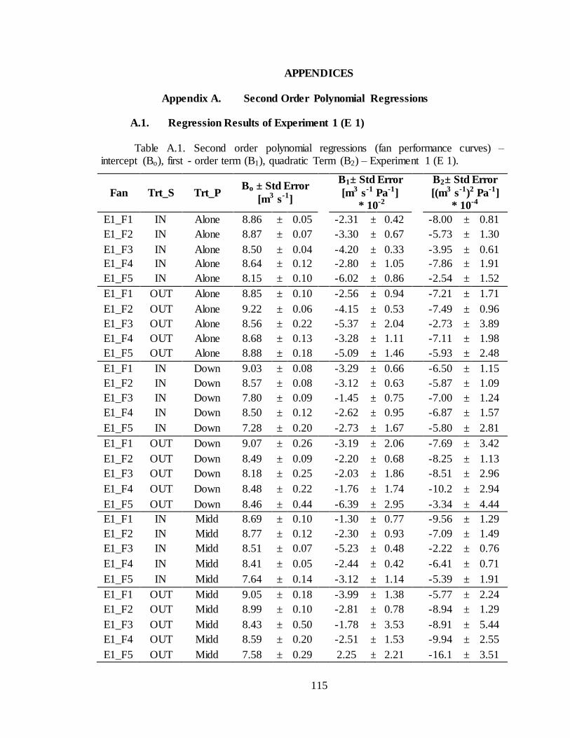
115
APPENDICES
Appendix A. Second Order Polynomial Regressions
A.1. Regression Results of Experiment 1 (E 1)
Table A.1. Second order polynomial regressions (fan performance curves) – intercept (Bo), first - order term (B1), quadratic Term (B2) – Experiment 1 (E 1).
Fan Trt_S Trt_P Bo ± Std Error
[m3 s-1]
B1± Std Error
[m3 s-1 Pa-1]
* 10-2
B2± Std Error
[(m3 s-1)2 Pa-1]
* 10-4
E1_F1 IN Alone 8.86 ± 0.05
-2.31 ± 0.42
-8.00 ± 0.81
E1_F2 IN Alone 8.87 ± 0.07
-3.30 ± 0.67
-5.73 ± 1.30
E1_F3 IN Alone 8.50 ± 0.04
-4.20 ± 0.33
-3.95 ± 0.61
E1_F4 IN Alone 8.64 ± 0.12
-2.80 ± 1.05
-7.86 ± 1.91
E1_F5 IN Alone 8.15 ± 0.10
-6.02 ± 0.86
-2.54 ± 1.52
E1_F1 OUT Alone 8.85 ± 0.10
-2.56 ± 0.94
-7.21 ± 1.71
E1_F2 OUT Alone 9.22 ± 0.06
-4.15 ± 0.53
-7.49 ± 0.96
E1_F3 OUT Alone 8.56 ± 0.22
-5.37 ± 2.04
-2.73 ± 3.89
E1_F4 OUT Alone 8.68 ± 0.13
-3.28 ± 1.11
-7.11 ± 1.98
E1_F5 OUT Alone 8.88 ± 0.18
-5.09 ± 1.46
-5.93 ± 2.48
E1_F1 IN Down 9.03 ± 0.08
-3.29 ± 0.66
-6.50 ± 1.15
E1_F2 IN Down 8.57 ± 0.08
-3.12 ± 0.63
-5.87 ± 1.09
E1_F3 IN Down 7.80 ± 0.09
-1.45 ± 0.75
-7.00 ± 1.24
E1_F4 IN Down 8.50 ± 0.12
-2.62 ± 0.95
-6.87 ± 1.57
E1_F5 IN Down 7.28 ± 0.20
-2.73 ± 1.67
-5.80 ± 2.81
E1_F1 OUT Down 9.07 ± 0.26
-3.19 ± 2.06
-7.69 ± 3.42
E1_F2 OUT Down 8.49 ± 0.09
-2.20 ± 0.68
-8.25 ± 1.13
E1_F3 OUT Down 8.18 ± 0.25
-2.03 ± 1.86
-8.51 ± 2.96
E1_F4 OUT Down 8.48 ± 0.22
-1.76 ± 1.74
-10.2 ± 2.94
E1_F5 OUT Down 8.46 ± 0.44
-6.39 ± 2.95
-3.34 ± 4.44
E1_F1 IN Midd 8.69 ± 0.10
-1.30 ± 0.77
-9.56 ± 1.29
E1_F2 IN Midd 8.77 ± 0.12
-2.30 ± 0.93
-7.09 ± 1.49
E1_F3 IN Midd 8.51 ± 0.07
-5.23 ± 0.48
-2.22 ± 0.76
E1_F4 IN Midd 8.41 ± 0.05
-2.44 ± 0.42
-6.41 ± 0.71
E1_F5 IN Midd 7.64 ± 0.14
-3.12 ± 1.14
-5.39 ± 1.91
E1_F1 OUT Midd 9.05 ± 0.18
-3.99 ± 1.38
-5.77 ± 2.24
E1_F2 OUT Midd 8.99 ± 0.10
-2.81 ± 0.78
-8.94 ± 1.29
E1_F3 OUT Midd 8.43 ± 0.50
-1.78 ± 3.53
-8.91 ± 5.44
E1_F4 OUT Midd 8.59 ± 0.20
-2.51 ± 1.53
-9.94 ± 2.55
E1_F5 OUT Midd 7.58 ± 0.29
2.25 ± 2.21
-16.1 ± 3.51

116
E1_F1 IN Opp.S. 8.66 ± 0.09
-1.92 ± 0.65
-9.07 ± 1.09
E1_F2 IN Opp.S. 8.88 ± 0.08
-4.22 ± 0.71
-4.04 ± 1.24
E1_F3 IN Opp.S. 8.09 ± 0.07
-3.61 ± 0.56
-3.85 ± 0.95
E1_F4 IN Opp.S. 8.34 ± 0.07
-3.89 ± 0.52
-5.24 ± 0.86
E1_F5 IN Opp.S. 7.65 ± 0.16
-3.22 ± 1.31
-5.63 ± 2.26
E1_F1 OUT Opp.S. 9.40 ± 0.08
-3.91 ± 0.60
-6.92 ± 0.99
E1_F2 OUT Opp.S. 8.72 ± 0.21
-3.89 ± 1.69
-6.00 ± 2.91
E1_F3 OUT Opp.S. 8.32 ± 0.37
-4.37 ± 2.98
-3.31 ± 4.93
E1_F4 OUT Opp.S. 8.98 ± 0.11
-5.47 ± 0.92
-7.15 ± 1.58
E1_F5 OUT Opp.S. 7.84 ± 0.26
-2.98 ± 2.05
-7.82 ± 3.38
E1_F1 IN S.S. 8.91 ± 0.06
-3.02 ± 0.50
-6.21 ± 0.85
E1_F2 IN S.S. 8.86 ± 0.05
-3.90 ± 0.43
-4.78 ± 0.73
E1_F3 IN S.S. 8.41 ± 0.06
-4.56 ± 0.44
-3.14 ± 0.73
E1_F4 IN S.S. 8.04 ± 0.32
-2.66 ± 2.53
-4.37 ± 4.00
E1_F5 IN S.S. 7.80 ± 0.11
-3.74 ± 0.89
-5.65 ± 1.49
E1_F1 OUT S.S. 8.97 ± 0.05
-3.66 ± 0.37
-5.99 ± 0.60
E1_F2 OUT S.S. 9.08 ± 0.11
-4.29 ± 0.89
-6.58 ± 1.51
E1_F3 OUT S.S. 8.22 ± 0.29
-2.91 ± 2.19
-6.13 ± 3.46
E1_F4 OUT S.S. 8.38 ± 0.20
-1.92 ± 1.54
-10.1 ± 2.53
E1_F5 OUT S.S. 8.24 ± 0.39
-2.88 ± 2.92
-9.10 ± 4.88
E1_F1 IN Up 8.15 ± 0.12
-3.61 ± 0.92
-3.47 ± 1.53
E1_F2 IN Up 8.23 ± 0.03
-3.76 ± 0.23
-2.91 ± 0.40
E1_F3 IN Up 7.05 ± 0.13
-0.06 ± 1.01
-7.57 ± 1.62
E1_F4 IN Up 7.33 ± 0.06
-0.43 ± 0.49
-8.72 ± 0.84
E1_F5 IN Up 7.21 ± 0.17
-5.37 ± 1.36
0.44 ± 2.28
E1_F1 OUT Up 8.54 ± 0.10
-3.01 ± 0.79
-5.86 ± 1.31
E1_F2 OUT Up 8.81 ± 0.15
-3.18 ± 1.15
-8.10 ± 1.90
E1_F3 OUT Up 8.37 ± 0.37
-4.18 ± 2.75
-4.58 ± 4.43
E1_F4 OUT Up 8.71 ± 0.08
-4.38 ± 0.63
-4.12 ± 1.08
E1_F5 OUT Up 8.06 ± 0.38
-4.66 ± 2.97
-5.02 ± 4.99
Treatments Abbreviation: IN (Inside), OUT (Outside), Down (Downstream), Midd
(Middle), Opp. S. (Opposite Sidewall), S.S. (Same Sidewall), Up (Upstream).

117
Table A.2. Second order polynomial regressions (fan performance curves) – coefficient of determination (R2), coefficient of variation, mean air flow rate, overall p-
value - Experiment 1 (E 1).
Fan Trt_S Trt_P R2 Coeff.
Var.
Root
MSE
[m3.s-1]
Mean Air
Flow [m3.s-1]
Overall
p-value
E1_F1 IN Alone 0.9982 0.71 0.05 7.58 <.0001
E1_F2 IN Alone 0.9948 1.28 0.10 7.56 <.0001
E1_F3 IN Alone 0.9992 0.54 0.04 7.02 <.0001
E1_F4 IN Alone 0.9936 1.66 0.12 7.10 <.0001
E1_F5 IN Alone 0.9958 1.56 0.10 6.29 <.0001
E1_F1 OUT Alone 0.9937 1.39 0.10 7.55 <.0001
E1_F2 OUT Alone 0.9987 0.80 0.06 7.38 <.0001
E1_F3 OUT Alone 0.9716 3.31 0.23 6.95 0.0001
E1_F4 OUT Alone 0.9923 1.80 0.13 7.03 <.0001
E1_F5 OUT Alone 0.9911 2.49 0.17 6.70 <.0001
E1_F1 IN Down 0.9979 0.79 0.06 7.46 <.0001
E1_F2 IN Down. 0.9977 0.77 0.05 7.10 <.0001
E1_F3 IN Down 0.9962 0.99 0.07 6.63 <.0001
E1_F4 IN Down 0.9958 1.21 0.08 7.01 <.0001
E1_F5 IN Down 0.9883 2.13 0.12 5.86 <.0001
E1_F1 OUT Down 0.9866 2.44 0.18 7.25 <.0001
E1_F2 OUT Down 0.9977 0.88 0.06 6.97 <.0001
E1_F3 OUT Down 0.9858 2.60 0.17 6.61 <.0001
E1_F4 OUT Down. 0.9895 2.21 0.15 6.87 <.0001
E1_F5 OUT Down 0.9758 3.87 0.23 6.00 <.0001
E1_F1 IN Midd 0.9972 0.84 0.06 7.35 <.0001
E1_F2 IN Midd 0.9957 1.17 0.08 7.25 <.0001
E1_F3 IN Midd 0.9987 0.64 0.04 6.71 <.0001
E1_F4 IN Midd 0.9990 0.50 0.03 7.02 <.0001
E1_F5 IN Midd 0.9935 1.51 0.09 6.15 <.0001
E1_F1 OUT Midd 0.9930 1.65 0.12 7.28 <.0001
E1_F2 OUT Midd 0.9982 0.90 0.06 7.18 <.0001
E1_F3 OUT Midd 0.9591 3.98 0.27 6.89 0.0003
E1_F4 OUT Midd 0.9921 1.98 0.14 6.85 <.0001
E1_F5 OUT Midd 0.9862 2.71 0.18 6.53 <.0001
E1_F1 IN Opp.S. 0.9977 0.95 0.07 7.02 <.0001
E1_F2 IN Opp.S. 0.9974 0.89 0.06 7.29 <.0001
E1_F3 IN Opp.S. 0.9974 0.83 0.06 6.65 <.0001
E1_F4 IN Opp.S. 0.9984 0.84 0.06 6.63 <.0001

118
E1_F5 IN Opp.S. 0.9892 2.14 0.13 6.12 <.0001
E1_F1 OUT Opp.S. 0.9984 0.84 0.06 7.54 <.0001
E1_F2 OUT Opp.S. 0.9859 2.34 0.16 7.04 <.0001
E1_F3 OUT Opp.S. 0.9567 3.89 0.26 6.70 0.0004
E1_F4 OUT Opp.S. 0.9981 1.23 0.08 6.67 <.0001
E1_F5 OUT Opp.S. 0.9876 2.75 0.17 6.07 <.0001
E1_F1 IN S.S. 0.9986 0.68 0.05 7.38 <.0001
E1_F2 IN S.S. 0.9989 0.57 0.04 7.21 <.0001
E1_F3 IN S.S. 0.9987 0.68 0.05 6.72 <.0001
E1_F4 IN S.S. 0.9546 3.90 0.26 6.67 0.0004
E1_F5 IN S.S. 0.9963 1.30 0.08 6.10 <.0001
E1_F1 OUT S.S. 0.9992 0.54 0.04 7.22 <.0001
E1_F2 OUT S.S. 0.9971 1.17 0.08 7.12 <.0001
E1_F3 OUT S.S. 0.9704 3.75 0.25 6.67 0.0002
E1_F4 OUT S.S. 0.9906 2.25 0.15 6.66 <.0001
E1_F5 OUT S.S. 0.9712 3.80 0.24 6.41 0.0001
E1_F1 IN Up 0.9939 1.14 0.08 6.80 <.0001
E1_F2 IN Up 0.9997 0.27 0.02 6.81 <.0001
E1_F3 IN Up 0.9908 1.42 0.09 6.27 <.0001
E1_F4 IN Up 0.9979 0.74 0.05 6.30 <.0001
E1_F5 IN Up 0.9895 1.63 0.09 5.69 <.0001
E1_F1 OUT Up 0.9962 1.01 0.07 7.03 <.0001
E1_F2 OUT Up 0.9952 1.58 0.11 6.98 <.0001
E1_F3 OUT Up 0.9684 3.56 0.24 6.61 0.0002
E1_F4 OUT Up 0.9981 0.75 0.05 7.00 <.0001
E1_F5 OUT Up 0.9705 3.93 0.24 6.13 0.0001
Treatments Abbreviation: IN (Inside), OUT (Outside), Downst. (Downstream), Midd (Middle), Opp. S. (Opposite Sidewall), S.S. (Same Sidewall), Up (Upstream).

119
A.2. Regression Results of Experiment 2 (E2)
Table A.3. Second order polynomial regressions (fan performance curves) – intercept (Bo), first - order term (B1), quadratic term (B2) – Experiment 2 (E 2).
Fan Trt_S Trt_P Bo ± Std Error
[m3 s-1]
B1± Std Error
[m3 s-1 Pa-1]
* 10-2
B2± Std Error
[(m3 s-1)2 Pa-1]
* 10-4
E2_F1 IN Alone 9.78 ± 0.14
-4.43 ± 1.22
-5.00 ± 2.37
E2_F2 IN Alone 9.75 ± 0.28
-4.47 ± 2.42
-4.38 ± 4.43
E2_F3 IN Alone 10.54 ± 0.17
-5.30 ± 1.59
-6.96 ± 2.96
E2_F4 IN Alone 10.44 ± 0.11
-6.00 ± 1.06
-5.37 ± 2.01
E2_F5 IN Alone 10.98 ± 0.07
-4.82 ± 0.65
-2.98 ± 1.26
E2_F1 OUT Alone 9.67 ± 0.29
-5.74 ± 2.88
-2.82 ± 5.91
E2_F2 OUT Alone 9.82 ± 0.21
-3.83 ± 1.76
-7.24 ± 3.09
E2_F3 OUT Alone 9.76 ± 0.11
-3.84 ± 1.00
-7.35 ± 1.95
E2_F4 OUT Alone 10.07 ± 0.29
-2.61 ± 2.29
-9.72 ± 3.83
E2_F5 OUT Alone 11.03 ± 0.07
-6.03 ± 0.65
-0.76 ± 1.24
E2_F1 IN Down 9.91 ± 0.28
-5.20 ± 2.18
-6.19 ± 3.61
E2_F2 IN Down 9.86 ± 0.14
-3.63 ± 1.07
-8.10 ± 1.79
E2_F3 IN Down 10.68 ± 0.19
-4.21 ± 1.69
-9.07 ± 3.09
E2_F4 IN Down 9.88 ± 0.10
-5.03 ± 0.80
-5.35 ± 1.39
E2_F5 IN Down 10.83 ± 0.16
-3.55 ± 1.30
-4.79 ± 2.22
E2_F1 OUT Down 9.56 ± 0.28
-3.50 ± 2.20
-7.56 ± 3.72
E2_F2 OUT Down 9.75 ± 0.14
-1.68 ± 1.08
-10.3 ± 1.82
E2_F3 OUT Down 9.64 ± 0.16
-0.94 ± 1.34
-13.1 ± 2.36
E2_F4 OUT Down 9.42 ± 0.34
-0.38 ± 2.61
-12.6 ± 4.31
E2_F5 OUT Down 11.02 ± 0.13
-3.74 ± 1.11
-3.78 ± 1.99
E2_F1 IN Midd 9.95 ± 0.19
-4.53 ± 1.48
-7.05 ± 2.53
E2_F2 IN Midd 9.13 ± 0.34
-1.04 ± 2.47
-10.2 ± 3.91
E2_F3 IN Midd 10.45 ± 0.17
-3.14 ± 1.36
-9.91 ± 2.36
E2_F4 IN Midd 9.75 ± 0.14
-3.95 ± 1.06
-6.48 ± 1.73
E2_F5 IN Midd 10.87 ± 0.14
-4.47 ± 1.00
-3.44 ± 1.60
E2_F1 OUT Midd 10.39 ± 0.32
-8.71 ± 2.46
-0.28 ± 4.06
E2_F2 OUT Midd 10.03 ± 0.34
-3.04 ± 2.55
-6.95 ± 4.18
E2_F3 OUT Midd 9.87 ± 0.38
-2.98 ± 3.00
-11.5 ± 5.06
E2_F4 OUT Midd 9.83 ± 0.40
-2.76 ± 2.91
-8.68 ± 4.67
E2_F5 OUT Midd 10.56 ± 0.16
-0.93 ± 1.17
-7.75 ± 1.88
E2_F1 IN Opp.S. 9.39 ± 0.14
-4.00 ± 1.16
-6.28 ± 2.06
E2_F2 IN Opp.S. 9.19 ± 0.33
-3.43 ± 2.56
-6.90 ± 4.15
E2_F3 IN Opp.S. 10.35 ± 0.07
-4.42 ± 0.57
-6.90 ± 0.99

120
E2_F4 IN Opp.S. 9.50 ± 0.10
-3.20 ± 0.87
-7.27 ± 1.51
E2_F5 IN Opp.S. 10.85 ± 0.06
-4.78 ± 0.42
-2.11 ± 0.69
E2_F1 OUT Opp.S. 10.05 ± 0.35
-2.28 ± 2.80
-11.6 ± 4.77
E2_F2 OUT Opp.S. 10.05 ± 0.25
-3.66 ± 2.04
-8.18 ± 3.56
E2_F3 OUT Opp.S. 9.71 ± 0.12
-2.27 ± 0.97
-10.3 ± 1.67
E2_F4 OUT Opp.S. 9.97 ± 0.22
-3.76 ± 1.79
-8.12 ± 3.09
E2_F5 OUT Opp.S. 10.64 ± 0.19
-4.98 ± 1.47
-2.56 ± 2.44
E2_F1 IN S.S. 9.93 ± 0.11
-6.29 ± 0.90
-4.13 ± 1.52
E2_F2 IN S.S. 9.66 ± 0.14
-0.62 ± 1.17
-12.5 ± 2.09
E2_F3 IN S.S. 10.33 ± 0.19
-2.97 ± 1.55
-10.7 ± 2.62
E2_F4 IN S.S. 9.66 ± 0.17
-2.51 ± 1.33
-9.23 ± 2.29
E2_F5 IN S.S. 10.82 ± 0.17
-4.94 ± 1.45
0.03 ± 2.56
E2_F1 OUT S.S. 9.51 ± 0.23
-1.14 ± 1.82
-11.5 ± 3.07
E2_F2 OUT S.S. 9.61 ± 0.46
-2.15 ± 3.32
-10.4 ± 5.27
E2_F3 OUT S.S. 9.96 ± 0.30
-5.45 ± 2.35
-5.59 ± 3.95
E2_F4 OUT S.S. 9.82 ± 0.29
-3.22 ± 2.17
-7.97 ± 3.56
E2_F5 OUT S.S. 10.60 ± 0.24
-3.87 ± 1.92
-3.06 ± 3.25
E2_F1 IN Up 8.86 ± 0.26
-5.78 ± 2.01
-3.65 ± 3.35
E2_F2 IN Up 9.36 ± 0.19
-8.01 ± 1.37
1.07 ± 2.14
E2_F3 IN Up 9.72 ± 0.10
-4.76 ± 0.76
-5.51 ± 1.22
E2_F4 IN Up 8.99 ± 0.11
-4.76 ± 0.77
-3.76 ± 1.22
E2_F5 IN Up 10.10 ± 0.18
-6.16 ± 1.27
0.56 ± 2.00
E2_F1 OUT Up 9.90 ± 0.38
-4.85 ± 2.83
-5.35 ± 4.62
E2_F2 OUT Up 8.90 ± 0.40
1.70 ± 2.84
-14.1 ± 4.52
E2_F3 OUT Up 10.09 ± 0.28
-4.59 ± 2.09
-6.94 ± 3.40
E2_F4 OUT Up 9.69 ± 0.45
-2.93 ± 3.27
-8.62 ± 5.16
E2_F5 OUT Up 9.98 ± 0.37
-1.71 ± 2.52
-7.37 ± 3.80
Treatments Abbreviation: IN (Inside), OUT (Outside), Downst. (Downstream), Midd (Middle), Opp. S. (Opposite Sidewall), S.S. (Same Sidewall), Up (Upstream).

121
Table A.4. Second order polynomial regressions (fan performance curves) – coefficient of determination (R2), coefficient of variation, mean air flow rate, overall p-
value - Experiment 1 (E 2).
Fan Trt_S Trt_P R2 Coeff.
Var.
Root
MSE
[m3.s-1]
Mean Air
Flow [m3.s-1]
Overall
p-value
E2_F1 IN Alone 0.9894 1.55 0.13 8.27 <.0001
E2_F2 IN Alone 0.9647 2.76 0.23 8.30 0.0002
E2_F3 IN Alone 0.9922 1.80 0.15 8.45 <.0001
E2_F4 IN Alone 0.9947 1.52 0.13 8.45 <.0001
E2_F5 IN Alone 0.9962 0.82 0.08 9.50 <.0001
E2_F1 OUT Alone 0.9485 3.76 0.31 8.13 0.0006
E2_F2 OUT Alone 0.9890 1.90 0.15 8.01 <.0001
E2_F3 OUT Alone 0.9933 1.52 0.12 8.16 <.0001
E2_F4 OUT Alone 0.9857 2.06 0.17 8.43 <.0001
E2_F5 OUT Alone 0.9962 0.86 0.08 9.37 <.0001
E2_F1 IN Down 0.9893 2.26 0.17 7.68 <.0001
E2_F2 IN Down 0.9956 1.34 0.11 7.93 <.0001
E2_F3 IN Down 0.9908 1.94 0.17 8.60 <.0001
E2_F4 IN Down 0.9974 0.94 0.07 7.93 <.0001
E2_F5 IN Down 0.9904 1.20 0.11 9.31 <.0001
E2_F1 OUT Down 0.9813 2.71 0.21 7.66 <.0001
E2_F2 OUT Down 0.9947 1.24 0.10 8.19 <.0001
E2_F3 OUT Down 0.9940 1.43 0.12 8.06 <.0001
E2_F4 OUT Down 0.9743 2.92 0.23 7.97 0.0000
E2_F5 OUT Down 0.9903 1.15 0.11 9.58 <.0001
E2_F1 IN Midd 0.9949 1.30 0.10 7.93 <.0001
E2_F2 IN Midd 0.9811 2.34 0.18 7.70 <.0001
E2_F3 IN Midd 0.9961 1.07 0.09 8.61 <.0001
E2_F4 IN Midd 0.9973 0.85 0.07 7.92 <.0001
E2_F5 IN Midd 0.9959 0.74 0.07 9.14 <.0001
E2_F1 OUT Midd 0.9868 2.29 0.18 7.79 <.0001
E2_F2 OUT Midd 0.9839 1.83 0.15 8.29 <.0001
E2_F3 OUT Midd 0.9854 2.56 0.20 7.83 <.0001
E2_F4 OUT Midd 0.9814 2.27 0.18 8.07 <.0001
E2_F5 OUT Midd 0.9927 0.92 0.09 9.43 <.0001
E2_F1 IN Opp.S. 0.9940 1.37 0.10 7.62 <.0001
E2_F2 IN Opp.S. 0.9771 3.13 0.23 7.42 <.0001
E2_F3 IN Opp.S. 0.9987 0.71 0.06 8.38 <.0001
E2_F4 IN Opp.S. 0.9963 1.09 0.09 7.85 <.0001

122
E2_F5 IN Opp.S. 0.9986 0.45 0.04 9.22 <.0001
E2_F1 OUT Opp.S. 0.9761 3.39 0.28 8.14 <.0001
E2_F2 OUT Opp.S. 0.9858 2.27 0.18 8.14 <.0001
E2_F3 OUT Opp.S. 0.9970 0.98 0.08 7.93 <.0001
E2_F4 OUT Opp.S. 0.9878 2.30 0.19 8.09 <.0001
E2_F5 OUT Opp.S. 0.9887 1.51 0.13 8.84 <.0001
E2_F1 IN S.S. 0.9973 1.11 0.08 7.67 <.0001
E2_F2 IN S.S. 0.9948 1.20 0.10 8.22 <.0001
E2_F3 IN S.S. 0.9929 1.87 0.16 8.36 <.0001
E2_F4 IN S.S. 0.9925 1.59 0.13 7.90 <.0001
E2_F5 IN S.S. 0.9790 1.47 0.14 9.47 <.0001
E2_F1 OUT S.S. 0.9857 2.46 0.19 7.91 <.0001
E2_F2 OUT S.S. 0.9678 3.54 0.28 7.79 0.0002
E2_F3 OUT S.S. 0.9834 2.55 0.20 7.83 <.0001
E2_F4 OUT S.S. 0.9786 2.71 0.22 8.07 <.0001
E2_F5 OUT S.S. 0.9743 1.86 0.17 9.14 0.0001
E2_F1 IN Up 0.9906 1.97 0.13 6.74 <.0001
E2_F2 IN Up 0.9948 1.29 0.09 7.03 <.0001
E2_F3 IN Up 0.9982 0.77 0.06 7.76 <.0001
E2_F4 IN Up 0.9981 0.76 0.05 7.14 <.0001
E2_F5 IN Up 0.9920 1.04 0.09 8.26 <.0001
E2_F1 OUT Up 0.9836 2.11 0.17 7.91 <.0001
E2_F2 OUT Up 0.9778 2.13 0.17 7.90 <.0001
E2_F3 OUT Up 0.9906 1.81 0.14 7.98 <.0001
E2_F4 OUT Up 0.9768 2.75 0.22 7.84 <.0001
E2_F5 OUT Up 0.9763 1.99 0.17 8.58 <.0001
Treatments Abbreviation: IN (Inside), OUT (Outside), Down (Downstream), Midd (Middle), Opp. S. (Opposite Sidewall), S.S. (Same Sidewall), Up (Upstream).

123
Appendix B. Statistical Results
B.1. Mixed Procedure Syntax used for Experiment 1 and 2
Table B.3. Mixed Procedure syntax for SAS® for analyzing the Generalized
Randomized Complete Block (GRCB) design.
PROC MIXED DATA=SASUSER.Experiment_1/2;
CLASS TRT_P TRT_S Fan;
MODEL AIRFLOW = TRT_P|TRT_S|SP;
RANDOM Fan;
LSMEANS TRT_S * TRT_P/DIFF;
RUN;

124
B.2. Mixed Procedure Results of Experiment 1 (E1)
Table B.1. Model information - SAS® output for Experiment 1 (E 1), using the Generalized Randomized Complete Block (GRCB) design.
Data Set SASUSER.E1
Dependent Variable Airflow
Covariance Structure Variance Components
Estimation Method REML
Residual Variance Method Profile
Fixed Effects SE Method Model-Based
Degrees of Freedom Method Containment
Covariance Parameters 2
Columns in X 42
Columns in Z 5
Subjects 1
Max Observations Per Subject 480
Number of Observations Read 480
Number of Observations Used 480
Number of Observations Not Used 0
Covariance Parameter Estimates
Covariance Parameters Estimate
Fan 0.1695
Residual 0.0561
Fit Statistics
-2 Res Log Likelihood 156.6
AIC (smaller is better) 160.6
AICC (smaller is better) 160.6
BIC (smaller is better) 159.8

125
Table B.2. SAS® Type III of fixed effects for Experiment 1 (E 1), using the Generalized Randomized Complete Block (GRCB) design.
Effect Num DF Den DF F Value Pr > F
Trt_P 5 452 15.43 <.0001
Trt_S 1 452 101.55 <.0001
Trt_P*Trt_S 5 452 5.16 0.0001
SP 1 452 9232.69 <.0001
SP*Trt_P 5 452 3.91 0.0018
SP*Trt_S 1 452 77.73 <.0001
SP*Trt_P*Trt_S 5 452 1.42 0.2150
Num, Den DF = Numerator, Denominator Degrees of Freedom .
Table B.3. Least Square Means estimates for Experiment 1 (E 1), using the Generalized Randomized Complete Block (GRCB) design in SAS®.
Effect Trt_P Trt_S Estimate
[m3.s-1]
Standard
Error
[m3.s-1]
DF t Value Pr >
|t|
Trt_P*Trt_S Alone IN 6.92 0.19 452 36.80 <.0001
Trt_P*Trt_S Alone OUT 7.00 0.19 452 37.21 <.0001
Trt_P*Trt_S Down IN 6.81 0.19 452 36.22 <.0001
Trt_P*Trt_S Down OUT 6.84 0.19 452 36.38 <.0001
Trt_P*Trt_S Midd. IN 6.94 0.19 452 36.94 <.0001
Trt_P*Trt_S Midd. OUT 6.99 0.19 452 37.19 <.0001
Trt_P*Trt_S Opp. S. IN 6.76 0.19 452 35.96 <.0001
Trt_P*Trt_S Opp. S. OUT 6.80 0.19 452 36.2 <.0001
Trt_P*Trt_S S. S. IN 6.86 0.19 452 36.52 <.0001
Trt_P*Trt_S S. S. OUT 6.88 0.19 452 36.59 <.0001
Trt_P*Trt_S Up IN 6.37 0.19 452 33.89 <.0001
Trt_P*Trt_S Up OUT 6.80 0.19 452 36.19 <.0001
DF = Degrees of Freedom. Treatments Abbreviation: IN (Inside), OUT (Outside), Down (Downstream), Midd (Middle), Opp. S. (Opposite Sidewall), S.S. (Same Sidewall), Up
(Upstream).

126
Table B.4. SAS® Least Square Means Difference output for Experiment 1 (E 1), using the Generalized Randomized Complete Block (GRCB) design.
Trt_P Trt_S Trt_P Trt_S Estimate
[m3.s-1]
Std.
Error
[m3.s-1]
DF p - value
Alone IN Alone OUT -0.08 0.05 452 0.1609
Alone IN Down IN 0.11 0.05 452 0.0362
Alone IN Midd. IN -0.02 0.05 452 0.6534
Alone IN Opp.
S. IN 0.16 0.05 452 0.0028
Alone IN S. S. IN 0.06 0.05 452 0.3005
Alone IN Up IN 0.56 0.05 452 <.0001
Alone OUT Down OUT 0.16 0.05 452 0.0034
Alone OUT Midd. OUT 0.01 0.05 452 0.9175
Alone OUT Opp.
S. OUT 0.20 0.05 452 0.0003
Alone OUT S. S. OUT 0.12 0.05 452 0.0278
Alone OUT Up OUT 0.19 0.05 452 0.0003
Down IN Down OUT -0.03 0.05 452 0.5672
Down IN Midd. IN -0.14 0.05 452 0.0105
Down IN Opp.
S. IN 0.05 0.05 452 0.3613
Down IN S. S. IN -0.06 0.05 452 0.2847
Down IN Up IN 0.44 0.05 452 <.0001
Down OUT Midd. OUT -0.15 0.05 452 0.0045
Down OUT Opp.
S. OUT 0.04 0.05 452 0.5082
Down OUT S. S. OUT -0.04 0.05 452 0.4567
Down OUT Up OUT 0.04 0.05 452 0.5060
Midd. IN Midd. OUT -0.05 0.05 452 0.3893
Midd. IN Opp.
S. IN 0.18 0.05 452 0.0005
Midd. IN S. S. IN 0.08 0.05 452 0.1352
Midd. IN Up IN 0.57 0.05 452 <.0001
Midd. OUT Opp.
S. OUT 0.19 0.05 452 0.0005
Midd. OUT S. S. OUT 0.11 0.05 452 0.0354
Midd. OUT Up OUT 0.19 0.05 452 0.0005
Opp.
S. IN
Opp.
S. OUT -0.04 0.05 452 0.4103
Opp. S.
IN
S. S.
IN
-0.11
0.05
452
0.0478

127
Opp. S.
IN Up IN 0.39 0.05 452 <.0001
Opp.
S. OUT S. S. OUT -0.08 0.05 452 0.1595
Opp.
S. OUT Up OUT 0.00 0.05 452 0.9969
S. S. IN S. S. OUT -0.01 0.05 452 0.8038
S. S. IN Up IN 0.49 0.05 452 <.0001
S. S. OUT Up OUT 0.08 0.05 452 0.1586
Up IN Up OUT -0.43 0.05 452 <.0001
DF = Degrees of Freedom. Treatments Abbreviation: IN (Inside), OUT (Outside), Down (Downstream), Midd (Middle), Opp. S. (Opposite Sidewall), S.S. (Same Sidewall), Up
(Upstream).

128
B.3. Mixed Procedure Results of Experiment 2 (E 2)
Table B.5. Model information - SAS® output for Experiment 2 (E 2), using the Generalized Randomized Complete Block (GRCB) design.
Data Set SASUSER.E2
Dependent Variable Airflow
Covariance Structure Variance Components
Estimation Method REML
Residual Variance Method Profile Fixed Effects SE Method Model-Based
Degrees of Freedom Method Containment
Covariance Parameters 2
Columns in X 42
Columns in Z 5
Subjects 1
Max Observations Per Subject 480
Number of Observations Read 480
Number of Observations Used 480
Number of Observations Not Used 0
Covariance Parameter Estimates
Covariance Parameters Estimate
Fan 0.313
Residual 0.097
Fit Statistics
-2 Res Log Likelihood 403.8
AIC (smaller is better) 407.8
AICC (smaller is better) 407.8
BIC (smaller is better) 407.0

129
Table B.6. SAS® Type III of fixed effects for Experiment 2 (E 2), using the Generalized Randomized Complete Block (GRCB) design.
Effect Num*
DF
Den*
DF
F
Value P > F
Trt_P 5 452 5.98 <.0001
Trt_S 1 452 3.47 0.0631
Trt_P*Trt_S 5 452 6.2 <.0001
SP 1 452 5943.1 <.0001
SP*Trt_P 5 452 0.43 0.8263
SP*Trt_S 1 452 0 0.9440
SP*Trt_P*Trt_S 5 452 1.24 0.2914
*Num, Den DF = Numerator, Denominator Degrees of Freedom .
Table B.7. Least Square Means estimates for Experiment 2 (E 2), using the
Generalized Randomized Complete Block (GRCB) design in SAS®.
Effect Trt_P Trt_S Estimate
[m3.s-1]
Standard
Error
[m3.s-1]
DF
t Value Pr >
|t|
Trt_P*Trt_S Alone IN 8.34 0.26 452 32.67 <.0001
Trt_P*Trt_S Alone OUT 8.23 0.26 452 32.25 <.0001
Trt_P*Trt_S Down IN 8.30 0.26 452 32.53 <.0001
Trt_P*Trt_S Down OUT 8.31 0.26 452 32.59 <.0001
Trt_P*Trt_S Midd. IN 8.31 0.26 452 32.59 <.0001
Trt_P*Trt_S Midd. OUT 8.38 0.26 452 32.86 <.0001
Trt_P*Trt_S Opp. S. IN 8.10 0.26 452 31.76 <.0001
Trt_P*Trt_S Opp. S. OUT 8.26 0.26 452 32.41 <.0001
Trt_P*Trt_S S. S. IN 8.31 0.26 452 32.6 <.0001
Trt_P*Trt_S S. S. OUT 8.19 0.26 452 32.11 <.0001
Trt_P*Trt_S Up IN 7.49 0.26 452 29.37 <.0001
Trt_P*Trt_S Up OUT 8.17 0.26 452 32.03 <.0001
DF = Degrees of Freedom. Treatments Abbreviation: IN (Inside), OUT (Outside), Down
(Downstream), Midd (Middle), Opp. S. (Opposite Sidewall), S.S. (Same Sidewall), Up (Upstream).

130
Table B.8. SAS® Least Square Means Difference output for Experiment 2 (E 2), using the Generalized Randomized Complete Block (GRCB) design.
Trt_P Trt_S Trt_P Trt_S Estimate
[m3.s-1]
Std.
Error
[m3.s-1]
DF p - value
Alone IN Alone OUT 0.11 0.07 452 0.1145
Alone IN Down IN 0.05 0.07 452 0.5262
Alone IN Midd. IN 0.03 0.07 452 0.6776
Alone IN Opp.
S. IN 0.24 0.07 452 0.0007
Alone IN S. S. IN 0.03 0.07 452 0.7138
Alone IN Up IN 0.85 0.07 452 <.0001
Alone OUT Down OUT -0.08 0.07 452 0.2363
Alone OUT Midd. OUT -0.15 0.07 452 0.0307
Alone OUT Opp.
S. OUT -0.04 0.07 452 0.6041
Alone OUT S. S. OUT 0.04 0.07 452 0.5792
Alone OUT Up OUT 0.06 0.07 452 0.4154
Down IN Down OUT -0.02 0.07 452 0.8228
Down IN Midd. IN -0.02 0.07 452 0.8255
Down IN Opp.
S. IN 0.20 0.07 452 0.0052
Down IN S. S. IN -0.02 0.07 452 0.7868
Down IN Up IN 0.81 0.07 452 <.0001
Down OUT Midd. OUT -0.07 0.07 452 0.3216
Down OUT Opp.
S. OUT 0.05 0.07 452 0.5020
Down OUT S. S. OUT 0.12 0.07 452 0.0801
Down OUT Up OUT 0.14 0.07 452 0.0448
Midd. IN Midd. OUT -0.07 0.07 452 0.3202
Midd. IN Opp.
S. IN 0.21 0.07 452 0.0026
Midd. IN S. S. IN -0.00 0.07 452 0.9603
Midd. IN Up IN 0.82 0.07 452 <.0001
Midd. OUT Opp.
S. OUT 0.12 0.07 452 0.0971
Midd. OUT S. S. OUT 0.19 0.07 452 0.0063
Midd. OUT Up OUT 0.21 0.07 452 0.0029
Opp.
S. IN
Opp.
S. OUT -0.16 0.07 452 0.0186
Opp. S.
IN
S. S.
IN
-0.21
0.07
452
0.0022

131
Opp. S.
IN Up IN 0.61 0.07 452 <.0001
Opp.
S. OUT S. S. OUT 0.08 0.07 452 0.2799
Opp. S.
OUT Up OUT 0.09 0.07 452 0.1802
S. S. IN S. S. OUT 0.13 0.07 452 0.0725
S. S. IN Up IN 0.82 0.07 452 <.0001
Up IN Up OUT -0.68 0.07 452 <.0001
DF = Degrees of Freedom. Treatments Abbreviation: IN (Inside), OUT (Outside), Down (Downstream), Midd (Middle), Opp. S. (Opposite Sidewall), S.S. (Same Sidewall), Up
(Upstream).

132
Appendix C. Barn Air Velocity Analysis
C.1. Results for Experiment 1 (E 1)
Table C.1. Model information and SAS® output for testing differences between
anemometers as a function of barn average air speed and treatments “P” - Proc GLM (Completely Randomized design – E 1).
Class Levels Values Number of Observations
Read/Used
TRT_P 5 Downstream Middle
Opposite Sidewall Same
Sidewall Upstream
200
R2 Coefficient
of Variation Root MSE [%]* Differences Mean [%]*
0.2371 1789.18 53.84 3.01
* % of mean air velocity from anemometers.
Table C.2. ANOVA table and Type III sums of squares for testing differences
between anemometers as a function of barn average air speed and treatments “P” - Proc GLM on SAS® (Completely Randomized design – E 1).
Source DF Sum of
Squares
Mean
Square
F -
Value P > F
Model 9 171227.82 19025.31 6.56 <0.0001
Error 190 550830.97 2899.11
Corrected Total 199 722058.80
Source DF Type III SS Mean
Square F Value P > F
Barn_AirSpeed 1 1154.67 1154.67 0.4 0.529
TRT_P 4 1831.00 457.75 0.16 0.959
Barn_AirSpeed*TRT_P 4 12699.93 3174.98 1.1 0.360

133
C.2. Results for Experiment 2 (E 2)
Table C.3. Model information and SAS® output for testing differences between anemometers as a function of barn average air speed and treatments “P” - Proc GLM (Completely Randomized design – E 2).
Class Levels Values Number of Observations
Read/Used
TRT_P 5
Downstream Middle
Opposite Sidewall Same Sidewall Upstream
200
R2 Coeff
Var Root MSE [%]* Differences Mean [%]*
0.2385 -364.27 44.81 -12.30
* % of mean air velocity from anemometers.
Table C.4. ANOVA table and Type III sums of squares for testing differences
between anemometers as a function of barn average air speed and treatments “P” - Proc GLM on SAS® (Completely Randomized design – E 2).
Source DF Sum of
Squares
Mean
Square F Value Pr > F
Model 9 119495.67 13277.30 6.61 <0.0001
Error 190 381486.33 2007.82
Corrected Total 199 500982.00
Source DF Type III
SS
Mean
Square F Value Pr > F
Barn_AirSpeed 1 19960.72 19960.72 9.94 0.002
TRT_P 4 11573.47 2893.37 1.44 0.222
Barn_AirSpeed*TRT_P 4 18872.11 4718.03 2.35 0.056

134
REFERENCES
Albright, L. D. 1990. Environment Control for Animals and Plants. St. Joseph, Mich.: ASAE.
Bottcher, R. W., G. R. Baughman and J. T. Magura. 1996. Field measurements of fan
speed and power use in poultry houses. Journal of Applied Poultry Research 5:
56-62.
Burns, R. T., H. Xin, R. S. Gates, H. Li, D. G. Overhults, L. Moody and J. W. Earnest. 2007. Ammonia emissions from broiler houses in the southeastern United States. In Proc. Int. Symp. Air Quality and Waste Management for Agriculture,
Broomfield, CO. Am. Soc. Agric. Biol. Eng., St. Joseph, MI.
Casey, K.D., J. R. Bicudo, D. R. Schmidt, A. Singh, S. W. Gay, R. S. Gates, L. D. Jacobson and S. J. Hoff. 2006. Air quality and emissions from livestock and poultry production/waste management systems. In: Rice, J.M., Caldwell, D.F.,
Humenik, F.J. (Eds.), Animal Agriculture and the Environment: National Center for Manure and Animal Waste Management White Papers. ASABE: Publ.
Number 913C0306, St. Joseph, MI. Casey, K.D., R.S. Gates, E.F. Wheeler, H. Xin, Y. Liang, A. Pescatore and M. Ford.
2008. On - farm ventilation fan performance evaluations and implications. Journal of Applied Poultry Research 17(2):283-295.
Casey, K.D., S.E. Ford, J.W. McClure, Y. Zhang and R.S. Gates. 2007. Determining fan
performance using FANS: an investigation of performance impacts. Applied
Engineering in Agriculture 23(3):333-338.
Chepete, H. J., H. Xin. 2002. Heat and Moisture Production of Poultry and Their Housing Systems – A Literature Review. In Livestock Environment VI Proceedings of the 6th International Symposium (21-23 May 2001, Louisville, Kentucky, USA).
ASAE. Publication Number 701P0201, Pp. 319-335.
Chepete, H. J., H. Xin. 2004. Ventilation Rates of a Laying Hen House Based on New vs. Old Heat and Moisture Production Data. Applied Engineering in Agriculture
20(6): 835−842.
Demmers, T. G. M., L. R. Burgess, J. L. Short, V. R. Phillips, J. A. Clark and C. M. Wathes. 1999. Ammonia emissions from two mechanically ventilated U.K. livestock buildings. Atmospheric Environ. 33(2): 217-227.
Gates, R. S., J. D. Simmons, K. D. Casey, T. Greis, H. Xin, E. F. Wheeler, C. King and J.
Barnett. 2002. Fan assessment numeration system (FANS) design and calibration specifications. Technical paper number 024124. American Society of Agricultural Engineers, St. Joseph, MI: ASAE.

135
Gates, R.S., K.D. Casey, H. Xin, E.F. Wheeler and J.D, Simmons. 2004. Fan assessment numeration system (FANS) design and calibration specifications. Transactions of
the ASAE 47(5):1709-1715.
Gates, R.S., K.D. Casey, H. Xin and R.T. Burns. 2009. Building emissions uncertainty estimates. Transactions of the ASABE 52(4):1345-1351.
Gates, R. S., H. Xin, K.D. Casey, Y. Liang and E.F. Wheeler. 2005. Method for measuring ammonia emissions from poultry houses. Journal of Applied Poultry
Research 14(3): 622-634. Gay, S.W., D.R. Schmidt, C.J. Clanton, K.A. Janni, L.D. Jacobson and S. Weisberg.
2003. Odor, total reduced sulfur, and ammonia emissions from animal housing facilities and manure storage units in Minnesota. Applied Engineering in
Agriculture 19(3) 347-360. Gay, S. W., E.F. Wheeler, J. L. Zajaczkowski and P. A. Topper. 2006. Ammonia
Emissions from U.S. Tom Turkey Growout and Brooder Houses Under Cold Weather Minimum Ventilation. Applied Engineering in Agriculture 22(1): 127-
134. Hoff, S.J., D.S. Bundy, M.A. Huebner, B.C. Zelle, L. D. Jacobson, B.P. Hetchler, V.J.
Johnson, R.E. Nicolai, D.R. Schmidt, P.R. Goodrich, A.J. Heber, J.Q. Ni, T.T. Lim, P.C. Tao, Y.Zhang, J. McClure, S. Jerez, M. Roberts, J.A. Koziel, B.H.
Baek, A. Balota, J.P. Spinhirne, J.M. Sweeten, D.B. Beasley, G.R. Baughman and R. Munilla. 2004. Real-Time Ventilation Measurements from Mechanically Ventilated Livestock Buildings for Emission Rate Estimations. ASAE Meeting
Paper No. 04-4178. St. Joseph, Mich.: ASAE.
Jacobson, L. D., A. J. Heber, J. M. Sweeten, J. Koziel, D. Bundy, S. Hoff, Y. Zhang, and R. W. Bottcher. 2001. Aerial pollutant emissions from animal confinement buildings. Proposal to USDA-IFAFS competitive grants program.
Janni, K. A., L. D. Jacobson, R. E. Nicolai, B. Hetchler and V. J. Johnson. 2005. Airflow
reduction of large belt-driven exhaust ventilation fans with shutters and loose belts. In Proc. 7th Int. Symp. Livest. Environ., Beijing, China, 245–251. Am. Soc. Agric. Eng., St. Joseph, MI.
Lacey, R. E., J. S. Redwine and C. B. Parnell Jr. 2003. Particulate matter and ammonia
emission factors for tunnel-ventilated broiler production houses in the southern U.S. Trans. ASAE 46(4): 1203-1214.
Li, H., H. Xin, S. Li and R. T. Burns. 2009. Downstream Placement of FANS to Determine Fan Performance in Situ. ASABE Paper No. 095886. 52(6): 2087-2090.

136
Li, H., H. Xin, R. T. Burns, L. D. Jacobson, S. Noll, S. J. Hoff, J. D. Harmon, J. A. Koziel, B. P. Hetchler. 2011. Air Emissions from Tom and Hen Turkey Houses in
the U.S. Midwest. Transactions of ASABE 54(1): 305-314.
Li, H., H. Xin, Y. Liang, R. S. Gates, E. F. Wheeler and A. J. Heber. 2005. Comparison of direct and indirect ventilation rate determinations in layer barns using manure belts. Transactions of the ASAE 48(1): 367–372.
Liang, Y., H. Xin, H. Li, R.S. Gates, E.F. Wheeler and K.D. Casey. 2005. Effect of
measurement interval on estimation of ammonia emission rates for layer houses. Transactions of the ASAE 49(1): 183-186.
Lim, T-T, J-Q Ni, A. J. Heber and Y. Jin. 2010. Applications and Calibrations of the FANS and Traverse Method for Barn Airflow Rate Measurement. International
Symposium on Air Quality and Manure Management for Agriculture, Proc. of the 13-16 September 2010 Conference, Dallas, Texas. Technical paper number: 711P0510cd.
Lima, K. A. O. 2011. Avaliação de Sistemas de Ventilação Mecanizada por Pressão
Positiva e Negativa Utilizados na Avicultura de Corte. Ph.D diss. Campinas, SP, Brazil: State University of Campinas (UNICAMP), Agricultural Engineering Department (FEAGRI).
Lopes, I. M., D. G. Overhults, G. M. Morello, J. Earnest Jr., R. S. Gates, A. Pescatore, J.
Jacob and M. Miller. 2010. Assessing Air Leakage in Commercial Broiler Houses. In 2010 ASABE Annual International Meeting, Pittsburgh, Pennsylvania. Technical paper number: 1009236.
Maghirang, R. G., Y. Liu and D. S. Chung. 1998. Evaluation of a freely rotating impeller to measure fan airflow rates in livestock buildings. Transactions of the ASAE 41(3): 819-824.
McQuiston, Faye C. 2005. Heating Ventilating, and Air Conditioning: Analysis and
Design. Faye C. McQuiston, Jerald D. Parker, Jeffrey D. Spitler – 6th ed. Hoboken, NJ: John Wiley & Sons, Inc.
Moody, L.B., H. Li, R.T. Burns, H. Xin, R. S. Gates, S.J. Hoff and D.G. Overhults. 2008. Southeastern Broiler Gaseous and Particulate matter Emissions Monitoring
Quality Assurance Project Plan. Published as Special ASABE peer reviewed publication..289.pages..ASABE,.St..Joseph,.MI.
Morello, G. M., D. G. Overhults, I. M. Lopes, J. Earnest Jr., R. S. Gates, A. Pescatore, J. Jacob and M. Miller. 2010. Influence of Fan Operations on FANS (Fan
Assessment Numeration System) Test Results. In: 2010 ASABE Annual

137
International Meeting, Pittsburgh, Pennsylvania. Technical paper number: 1009235.
Ni, J.-Q., A. J. Heber, T. T. Lim, R. Duggirala, B. L. Haymore, C. A. Diehl and A. L.
Sutton. 1998a. Hydrogen sulfide emissions from a large mechanically-ventilated swine building during warm weather. St. Joseph, Mich.: ASAE. Technical paper number: 984051
Ni, J.-Q., A. J. Heber, T. T. Lim, R. Duggirala, B. L. Haymore, C. A. Diehl and A. L.
Sutton. 1998b. Ammonia emission from a large mechanically-ventilated swine building during warm weather. St. Joseph, Mich.: ASAE. Technical paper number: 984051
Phillips, V. R., M. R. Holden, R. W. Sneath, J. L. Short, R. P. White, J. Hartung, J.
Seedorf, Schro der M, K. H. Linkert, S. Pedersen, H. Takai, J. O. Johnsen, P. W. G. Groot Koerkamp, G. H. Uenk, R. Scholtens, J. H. M. Metz and C. M. Wathes. 1998. The development of robust methods for measuring concentrations and
emission rates of gaseous and particulate air pollutants in livestock buildings. Journal of Agricultural Engineering Research, 70:11–24.
Sama, M. P., R. S. Gates, W. C. Adams, G. B. Day and C. L. King. 2008. Fans
Assessment Numeration System (FANS) Scaling and Upgrades. ASABE Annual
International Meeting 2008, Paper number 084723.
Simmons, J.D., T.E. Hannigan and B.D. Lott. 1998a. A portable anemometer to determine the output of large in-place ventilation fans. Applied Engineering in Agriculture, 14(6):649-653.
Simmons, J. D., B. D. Lott and T.E. Hannigan. 1998b. Minimum distance between
ventilation fans in adjacent walls of tunnel ventilated broiler houses. Applied Eng. In Agric. 14(5): 533 - 535.
Topper, P. A., E. F. Wheeler, J. S. Zajaczkowski, R. S. Gates, H. Xin, Y. Liang and K. D. Casey. 2008. Ammonia emissions from two empty broiler houses with built-up
litter. Trans. Am. Soc. Agric. Biol. Eng. 51:219–225. Wang, L, Y. Jin and B. Cui. 2010. Factors affecting small axial cooling fan performance.
Journal of thermal science (19):126-131.
Wheeler, E.F., K.D. Casey, R.S. Gates, H. Xin, J.L. Zajaczkowski, P.A. Topper, Y. Liang and A.J. Pescatore. 2006. Ammonia emissions from twelve U.S.A. broiler houses. Transactions of the ASABE 49(5):1495-1512.
Wheeler, E. F., K. D. Casey, J. S. Zajaczkowski, P. A. Topper, R. S. Gates, H. Xin, Y.
Liang. and A Tanaka. 2003. Ammonia emissions from U.S. poultry houses: Part

138
III – Broiler houses. In: Proc. Air Pollution Agric. Operations III Conf., Research Triangle Park, NC. ASAE Publ. No. 701P1403. ASAE, St. Joseph, MI. 159–166.
Xin, H., H. Li, R. T. Burns, R. S. Gates, D. G. Overhults, J. W. Earnest. 2009. Use of
CO2 Concentration Difference or CO2 Balance to Assess Ventilation Rate of Broiler Houses. Transactions of ASABE 52(4): 1353-1361.
Zar, J. H. 2006. Biostatistical Analysis. 4th edition, New Delhi, India: Pearson Education.
Zhu, J., L. D. Jacobson, D. R. Schmidt and R. E. Nicolai. 2000. Daily variations in odor and gas emissions from animal facilities. Transactions of the ASAE 16(2): 153–158.

139
VITA
Gabriela Munhoz Morello
Date and Place of Birth: 04/22/1986,
Campinas, SP, Brazil.
Education:
03/2004 – 12/2008
UNICAMP, State University, Campinas - SP, Brazil, Agricultural Engineering
College. One Scientific Initiation (one year research program) in post harvesting,
under supervision of Dr. Inácio Maria Dal Fabro. Project title:
“Application of the Dynamic Speckle Technique to Seed Viability Analysis”.
Three Scientific Initiations (one year research programs) in broiler and turkey production, under supervision of Dr. Daniella J. de Moura. Project
titles:
“Effect of environment temperature, relative humidity and air
velocity on turkey wattle temperatures”;
“Investigation of ammonia concentration in broiler houses
equipped with negative pressure fans (exhaust fans) and positive pressure fans ”;
“Study of water consumption and quality as indicators of
welfare of broiler chickens”.
ITAL – Istitute of Food Technology.
Course of auditing swine and poultry welfare in slaughter
houses and production facilities.
01/ 2010 - 08/2011
Masters Program in the Biosystems and Agricultural Engineering dpt., University of Kentucky, under supervision of Dr. Douglas G. Overhults. Project
title:
“Influence of Operating Fans inside Poultry Houses on FANS
(Fan Assessment Numeration System) Test Results”.
140
Work Experience:
January – December 2009
Research Assistant at the Research and Education Center, University of Kentucky.
Worked on the project “Poultry House Evaluation Service (PHES)”, 2009.
July – December, 2008 Avícola Paulista, Louveira – SP, Brazil
Internship in agricultural extension activity in broiler housings and feed raw material analysis (quality control sector).
July – October, 2006 Sadia S/A, Concórdia – SC, Brazil
Internship in agricultural extension activity in broiler houses.
Awards and Achievements:
- The Outstanding Graduate M.S. Student, by the Honor Society of Agriculture Gamma Sigma Delta, University of Kentucky Chapter (March/2011);
- Outstanding Project Award, in recognition of Kentucky Poultry Energy Efficiency Project – Kentucky Association of State Extension Professionals (March/2011).
- One of the top three Agricultural Engineering Graduates of January 2008, UNICAMP.
Publications:
Journals:
Morello G.M., A. S. Mende, D. J. Moura. 2007. Efeito da Velocidade do Vento na
Temperatura de Barbela de Perus aos 61 dia (Effect of Air Velocity on Wattle Temperature of 61 Day Old Turkeys). Revista Brasileira de Ciência Avícola /
Brazilian Journal of Poultry Science , 9:17-18. Mendes A. S., D. J. Moura, T. M. R. Carvalho; G. M. Morello, I. A. Naas. 2008.
Resposta fisiológica de perus de distintas idades em conforto vs. estresse térmico (Physiological Responses of Turkeys of Different Ages when in Comfort vs.
Stress). Revista Brasileira de Ciência Avícola / Brazilian Journal of Poultry Science , 10: 26-27.

141
Naas I. A., L. T. Sonoda, C. E. B. Romanini, G. M. Morello, M. S. Baracho, S. R. L. Souza, A. G. Menezes, M. Mollo, D. J. Moura. 2008. Morphological asymmetry
and broiler welfare. Revista Brasileira de Ciência Avícola / Brazilian Journal of Poultry Science , 10:203-207.
Conferences:
Morello G. M., S. Rodrigues, I. M. Dal Fabbro, B. Rebôlla. 2006. Teste de Tetrazólio e sua Eficácia na Identificação da Viabilidade de Sementes e Danos Decorrentes do
Processo Agrícola (Tetrazolium Test and its Efficacy on Identifying Seed Viability and Damages due to the Agricultural Process). In: XXXV Congresso Brasileiro de Engenharia Agrícola, 2006, João Pessoa, PB. XXXV Congresso
Brasileiro de Engenharia Agrícola. Jaboticabal-SP : SBEA, 2006. v. 1.
Morello, G.M., A. S. Mendes, D. J. Moura. 2008. Effect of wind speed over Turkey s wattle temperature in turkeys aged 61, 96 and 131 days old. In: 2008 ASABE Annual international Meeting St. Joseph.
Morello G. M., L. T. Sonoda, D. J. Moura. 2008. Influência da Ventilação Mecânica na
Produção de Amônia em Galpões para Produção de Frangos de Corte (Influence of the Mechanical Ventilation on Ammonia Concentrations in Broiler Houses). In: Conferência APINCO 2008, Santos, SP. 10: 27-27.
Morello G. M., L. T. Sonoda, D. J. Moura. 2008. Estudo da Interação entre as Variáveis
Climáticas e a Concentração de Amônia em Galpões de Confinamento para Frangos de Corte (Study of the Influence of Climatic Variables and the Ammonia Concentration in Broiler Houses). In: Seminário de Mudanças Climáticas na
Produção Animal, Campinas, SP. 1: 33-33.
Morello G. M., D. G. Overhults, I. L. Lopes, J. Earnest Jr., R. S. Gates, A. Pescatore, J. Jacob, M. Miller. 2010. Influence of Fan Operations on FANS (Fan Assessment Numeration System) Test Results. In: 2010 ASABE Annual International
Meeting, Pittsburgh, Pennsylvania. Technical paper number: 1009235.
Rodrigues S., G. M. Morello, I. M. Dal Fabbro, G. F. Rabelo, A. M. Enes. 2005. Application of The Dynamic Speckle Technique to Seed Viability Analysis. In: International Congress on Information Technology in Agriculture, Food and
Environment, ITAFE05, 2005, Turkey: Çukurova University, Adana. II: 777-780.
Rodrigues S., I. M. Dal Fabbro, B. Rebôlla, G. M. Morello. 2006. Application of Dynamic Speckle Techniques in Seed Viability Sorting. The Annual Meeting and an International Conference in Collaboration with the "Agritech 2006"
Exhibition, 2006, Tel Aviv: ISAE - The Israeli Society of Agricultural Engineers.
Mendes A. S., S. J. Paixão, G. M. Morello, J. Marostega, R. Restelatto. 2010. Resposta comportamental de perus em diferentes condições climáticas (Behavioral

142
Responses of Turkeys at Different Environment Conditions). In: Avisulat 2010, Bento Gonçalves. II Congresso Sul Brasileiro de Avicultura, Suinocultura e
Laticínios. 1: 1-1.
Sonoda L. T., G. M. Morello, D. J. Moura, J. W. Pinheiro.2008. Concentrações de amônia em Fução das Condições da Cama para dois Sistemas de Ventilação Mecânica na Produção de Frangos de Corte (Ammonia Concentrations as a
Function of Bedding Characteristics). In: Conferência Apinco 2008, Santos, SP. Campinas: FACTA, 2008. 10: 26-26.
Sonoda L. T., G. M. Morello, D. J. Moura, J. W. Pinheiro.2008. Comparação de Dois
Diferentes Sistemas de Ventilação Mecânica em Galpões de Frango de Corte para
Avaliação das Concentrações de NH3 em Função das Condições da Cama (Comparing the Bedding Characteristics and Ammonia Concentrations in Broiler
Houses with Different Ventilation Systems). In: Seminário de Mudanças Climáticas e a Produção Animal, 2008, Campinas. 1: 15-15.
Lopes I. M., D. G. Overhults, G. M. Morello, J. Earnest Jr., R. S. Gates, A. Pescatore, J. Jacob and M. Miller. 2010. Assessing Air Leakage in Commercial Broiler
Houses. In 2010 ASABE Annual International Meeting, Pittsburgh, Pennsylvania. Technical paper number: 1009236
Rebôlla B., S. Rodrigues, I. M. Dal Fabbro, G. M. Morello. Tempo de Cocção em Função do Tempo de Envelhecimento para Grãos de Feijão (Influence of Artificial Aging
of Beans on their Cook Time).2006. In: XXXV Congresso Brasileiro de Engenharia Agrícola, 2006, João Pessoa, PB. Congresso Brasileiro de Engenharia Agrícola. Jaboticabal-SP : SBEA, 2006. v. 1.
Mendes A. S., D. J. Moura, G. M. Morello, T. M. R. Carvalho.2008. Alterações na
Temperatura de Barbela de Perus Submetidos a Distintas Condições Climáticas (Alterations on Turkey Wattle Temperature under Different Environment Conditions). In: Sistemas de Produção Agropecuária, 2008, Dois Vizinhos,
UTFPR. 1: 66-69.
Morello G.M., D. J. Moura, A. D. Mendes. Efeito da Velocidade do Vento na Temperatura de Barbela de Perus aos 96 Dias (Effect of wind speed over Turkey wattle temperature in turkeys aged 61, 96 and 131 days old). 2007. In: XXXVI
Congresso Brasileiro de Engenharia Agrícola, Bonito, MT. p. 1-4.
Morello G. M., L. T. Sonoda, D. J. Moura. 2008. Estudo da Interação entre as Variáveis Climáticas e a Concentração de Amônia em Galpões de Confinamento para Frangos de Corte (Study of the Interaction of Environmental Variables and
Ammonia Concentrations in Broiler Houses). In: Seminário de Mudanças Climáticas na Produção Animal, 2008, Campinas. Anais do Seminário de
Mudanças Climáticas na Produção Animal. 1: 33-33.

143
Morello G. M., D. J. Moura. 2008. Estudo da Influência da Ventilação Mecânica no Bem-Estar e na Produtividade de Frangos de Corte (Study of the Influence of
Mechanical Ventilation on Broiler Welfare and Productivity). In: PIBIC-XVI Congresso Interno de Iniciação Científica, Campinas, SP. 1: T0935-T0935.
Morello G. M., A. S. Mendes, D. J. Moura. 2007. Efeito da Velocidade do Vento na
Temperatura de Barbela de Perus aos 61 dias (Effect of Air Velocity on Wattle
Temperature of 61 Day Old Turkeys). In: Conferência Apinco de Ciência e Tecnologia Avícolas, 2007, Santos, SP. 9: 17-17.
Morello G. M., D. J. Moura. 2007. Efeito da Velocidade do Vento na Temperatura de
Barbela de Perus aos 61, 96 e 131 dias (Effect of wind speed over Turkey wattle
temperature in turkeys aged 61, 96 and 131 days old). In: PIBIC- XV Congresso Interno de Iniciação Científica, Campinas, SP. 1: T0805-T0805.
Morello G. M., S. Rodrigues, I. M. Dal Fabbro. 2006. Aplicação da Técnica do Speckle
Dinâmico no Estudo da Viabilidade de Sementes de Feijão ( Phaseolus vulgaris,
L) (Study of the Application of the Dynamic Speckle Techinique on Bean Seed Viabilities). In: XIV Congresso Interno de Iniciação Científica da UNICAMP,
Campinas, SP. Overhults, D.G., A. Pescatore, I.M. Lopes, G.M. Morello, J.P. Jacob, M. Miller, J.W.
Earnest, Jr., and R.S. Gates. 2010. Air velocities in poultry houses raising large broilers. 2010 Poultry Science Association Annual Meeting. Poultry Science 89
(Supp. 1). Overhults, D.G., A. Pescatore, I.M. Lopes, G.M. Morello, J.P. Jacob, J.W. Earnest, Jr.,
M. Miller, and R.S. Gates. 2010. Overview of lighting in Kentucky broiler houses. 2010 Poultry Science Association Annual Meeting. Poultry Science
89(Supp. 1). Overhults, D.G., A. Pescatore, I.M. Lopes, G.M. Morello, J.W. Earnest, Jr., M. Miller,
J.P. Jacob, and R.S. Gates. 2010. Using thermal imaging for poultry house energy assessments. International Poultry Scientific Forum, Southern Poultry
Science Society Meeting Abstracts, p. 49.
Gabriela Munhoz Morello
06/15/2011