This Bachelor’s Thesis is carried out as a part of the education at the

University of Agder and is therefore approved as a part of this

education. However, this does not imply that the University answers

for the methods that are used or the conclusions that are drawn.

University of Agder, 2016

Faculty of Engineering and Science

Department of Engineering Sciences

Implementing SLAM on a Differential Drive

AGV

Ørjan Langøy Olsen,

Øystein Øihusom

Supervisor

Morten Ottestad

Ørjan Langøy Olsen Øystein Øihusom

AbstractAutonomous robots have a potential in many different areas. Care of the elderly, warehouses and cleaning

of buildings to mention a few. University of Agder wants to automate mapping of areas for the use of robotsusing simultaneous localization and mapping (SLAM). SLAM is a technique for building a map of an unknownenvironment while at the same time determine own position. A differential drive robot was built for this project toexecute the SLAM technique. Its design was modelled in Solid Works with rapid prototyping and modularity inmind. The plastic parts were printed with ABS plastic using a CubePro 3D printer. National Instrument myRIOwas used as the microcontroller and the program code was written in LabVIEW G code. The robot uses sensorfusion to determine its position by combining the odometry from motor encoders and landmark positions sensedby a laser scanner. Multiple navigation behaviors were implemented for safe and reliable obstacle avoidance aswell as maneuvering to a goal by employing multiple waypoints. After building and programming of the robot,tests were performed in both software and hardware to increase the accuracy and robustness during operation.When performing the full system test, the robot performed as expected. It mapped the assigned area, but whenit returned to a previously visited location, the registered position was not the same. This is because of theloop-closure problem, which is not handled in this project.

LIST OF FIGURES LIST OF TABLES

List of Figures1 Global coordinate system and reference frame for the robot. . . . . . . . . . . . . . . . . . . . . . . . 92 Estimating position from previous position, motion model, encoder position and observation data. . 103 Illustration of quadrature encoder channels. (Robot Builder’s Bonanza, 4th Edition - Application

Notes & Bonus Projects Copyright © 2011, Gordon McComb) . . . . . . . . . . . . . . . . . . . . . 124 Block diagram illustration of the complementary filter. . . . . . . . . . . . . . . . . . . . . . . . . . . 135 Block diagram illustration of the SLAM process. . . . . . . . . . . . . . . . . . . . . . . . . . . . . . 156 Sensor frame S offset relative to robot frame R. . . . . . . . . . . . . . . . . . . . . . . . . . . . . 197 A rotating mirror is used to take distance measurements in the plane. . . . . . . . . . . . . . . . . . 238 The effect of outliers on the least squares method. . . . . . . . . . . . . . . . . . . . . . . . . . . . . 239 Line between two randomly selected points. . . . . . . . . . . . . . . . . . . . . . . . . . . . . . . . . 2410 Amount of inliers are counted for the line. . . . . . . . . . . . . . . . . . . . . . . . . . . . . . . . . . 2411 The correct line will eventually be found. . . . . . . . . . . . . . . . . . . . . . . . . . . . . . . . . . 2412 A line is drawn between the two most distant points. . . . . . . . . . . . . . . . . . . . . . . . . . . . 2513 The most distant point from the line is within a given threshold, so a split is performed. . . . . . . . 2514 The contour after no more splits can be made. . . . . . . . . . . . . . . . . . . . . . . . . . . . . . . 2515 Two of the line segments are collinear enough to merge them. . . . . . . . . . . . . . . . . . . . . . . 2616 A previously visited location is not registered at the same position, illustrating the loop closure problem. 2617 The number on the nodes tells in which order they were visited. . . . . . . . . . . . . . . . . . . . . . 2718 A graph being explored by Dijkstras. The second letter is the node it came from. . . . . . . . . . . . 2819 First robot design. . . . . . . . . . . . . . . . . . . . . . . . . . . . . . . . . . . . . . . . . . . . . . . 3120 Second robot design. . . . . . . . . . . . . . . . . . . . . . . . . . . . . . . . . . . . . . . . . . . . . . 3221 Computer generated imagery. . . . . . . . . . . . . . . . . . . . . . . . . . . . . . . . . . . . . . . . . 3322 . . . . . . . . . . . . . . . . . . . . . . . . . . . . . . . . . . . . . . . . . . . . . . . . . . . . . . . . . 3723 Inputs and outputs of the motor control VI. . . . . . . . . . . . . . . . . . . . . . . . . . . . . . . . . 3724 Code for controlling a motor. . . . . . . . . . . . . . . . . . . . . . . . . . . . . . . . . . . . . . . . . 3825 LabView code for LIDAR data acquisition. . . . . . . . . . . . . . . . . . . . . . . . . . . . . . . . . 3926 Lines extracted from sample data with the RANSAC algorithm. . . . . . . . . . . . . . . . . . . . . 4027 Lines extracted from sample data with the split and merge algorithm. . . . . . . . . . . . . . . . . . 4128 How landmarks are selected. . . . . . . . . . . . . . . . . . . . . . . . . . . . . . . . . . . . . . . . . . 4229 Block diagram illustration of the SLAM process. . . . . . . . . . . . . . . . . . . . . . . . . . . . . . 4330 Graphical representation of the state vector used in EKF SLAM . . . . . . . . . . . . . . . . . . . . 4431 Dimensions of the state vector and covariance matrix. . . . . . . . . . . . . . . . . . . . . . . . . . . 4432 Prediction step applied to state vector and covariance matrix. . . . . . . . . . . . . . . . . . . . . . . 4633 EKF SLAM prediction step, MathScript node. . . . . . . . . . . . . . . . . . . . . . . . . . . . . . . 4734 Update step applied to state vector and covariance matrix. . . . . . . . . . . . . . . . . . . . . . . . 4835 New landmark expanding the state vector and covariance matrix. . . . . . . . . . . . . . . . . . . . . 4936 An occupancy grid map represented visually. . . . . . . . . . . . . . . . . . . . . . . . . . . . . . . . 5037 PID tuning two motors on a differential drive. . . . . . . . . . . . . . . . . . . . . . . . . . . . . . . . 5238 Comparison between RANSAC and Split and Merge. . . . . . . . . . . . . . . . . . . . . . . . . . . . 5539 Results from testing the robot . . . . . . . . . . . . . . . . . . . . . . . . . . . . . . . . . . . . . . . 5640 Converting an array of cartesian coordinates to polar coordinates using the in-place element. . . . . 58

List of Tables1 Clockwise rotations . . . . . . . . . . . . . . . . . . . . . . . . . . . . . . . . . . . . . . . . . . . . . . 112 Counterclockwise rotations . . . . . . . . . . . . . . . . . . . . . . . . . . . . . . . . . . . . . . . . . 113 Motor specifications. . . . . . . . . . . . . . . . . . . . . . . . . . . . . . . . . . . . . . . . . . . . . . 344 Overview of input and output voltage of the voltage regulators. . . . . . . . . . . . . . . . . . . . . . 355 Results from the straight line test. . . . . . . . . . . . . . . . . . . . . . . . . . . . . . . . . . . . . . 52

4

LIST OF TABLES LIST OF TABLES

6 Results from rotation test. . . . . . . . . . . . . . . . . . . . . . . . . . . . . . . . . . . . . . . . . . . 537 Results from the square drive test. . . . . . . . . . . . . . . . . . . . . . . . . . . . . . . . . . . . . . 548 Results from the LIDAR test. . . . . . . . . . . . . . . . . . . . . . . . . . . . . . . . . . . . . . . . . 549 RANSAC parameters used during testing. . . . . . . . . . . . . . . . . . . . . . . . . . . . . . . . . . 5510 Split and Merge parameters used during testing. . . . . . . . . . . . . . . . . . . . . . . . . . . . . . 55

NomenclatureA* A popular pathfinding algorithm using graph traversal.

AGV Automated Guided Vehicle

Algorithm A step-by-step set of operations to be performed to arrive at a solution or complete a task.

Clustering The act of seperating data into clusters.

Differential drive Drive system where two seperately driven wheels placed on either side of the robot controls themovement.

Graph Mathematical structures used to model pairwise relations between objects.

Heuristic Method for solving problems utilizing a set of rules.

Inlier Points with a residual less than a given threshold.

Landmark (LMK) Features in the map. For example wall, corner or pillar.

LIDAR Portmanteau of light and radar and is a radial distance sensor.

Linestrip A list of vertices where the first issued vertex begins the linestrip and every consecutive vertexmarks a joint in the line.

LiPo Lithium polymer battery.

Occupancy grid A binary map that tells wheter a given space is occupied or not.

Odometry The use of motion sensors to estimate position.

Outliers Points with a residual greater than a given threshold.

PID A controller that tries to minimize the difference between a desired setpoint and a measuredprocess variable using a gain, integral and derivative term.

Process variable The variable being regulated in a control system.

RANSAC Random sample consensus. An algorithm for approximating a line from a set of points.

Residuals The difference between an observed value and the fitted value provided by a model.

Sensor fusion Combination of sensory data from seperate sources such that the resulting information has lessuncertainty than the individual sources.

Setpoint The desired value for a process variable.

SLAM Simultaenous Localization and Mapping

SubVI Function block in LabVIEW. It can take multiple inputs and return multiple outputs.

Vertex A point in a geometric figure.

5

CONTENTS CONTENTS

Contents1 Introduction 8

2 Theory 92.1 Locomotion . . . . . . . . . . . . . . . . . . . . . . . . . . . . . . . . . . . . . . . . . . . . . . . . . . 92.2 Kinematics . . . . . . . . . . . . . . . . . . . . . . . . . . . . . . . . . . . . . . . . . . . . . . . . . . 9

2.2.1 Kinematics . . . . . . . . . . . . . . . . . . . . . . . . . . . . . . . . . . . . . . . . . . . . . . 92.2.2 Probabilistic kinematics . . . . . . . . . . . . . . . . . . . . . . . . . . . . . . . . . . . . . . . 102.2.3 Motion models . . . . . . . . . . . . . . . . . . . . . . . . . . . . . . . . . . . . . . . . . . . . 10

2.3 Complementary filter . . . . . . . . . . . . . . . . . . . . . . . . . . . . . . . . . . . . . . . . . . . . . 132.4 SLAM with complementary filter . . . . . . . . . . . . . . . . . . . . . . . . . . . . . . . . . . . . . . 142.5 Extended Kalman filter . . . . . . . . . . . . . . . . . . . . . . . . . . . . . . . . . . . . . . . . . . . 162.6 SLAM with extended Kalman filter . . . . . . . . . . . . . . . . . . . . . . . . . . . . . . . . . . . . . 172.7 Laser scanner . . . . . . . . . . . . . . . . . . . . . . . . . . . . . . . . . . . . . . . . . . . . . . . . . 222.8 Line extraction . . . . . . . . . . . . . . . . . . . . . . . . . . . . . . . . . . . . . . . . . . . . . . . . 23

2.8.1 RANSAC . . . . . . . . . . . . . . . . . . . . . . . . . . . . . . . . . . . . . . . . . . . . . . . 232.8.2 Split and merge . . . . . . . . . . . . . . . . . . . . . . . . . . . . . . . . . . . . . . . . . . . . 25

2.9 Loop closure . . . . . . . . . . . . . . . . . . . . . . . . . . . . . . . . . . . . . . . . . . . . . . . . . 262.10 A* search algorithm . . . . . . . . . . . . . . . . . . . . . . . . . . . . . . . . . . . . . . . . . . . . . 272.11 Navigation . . . . . . . . . . . . . . . . . . . . . . . . . . . . . . . . . . . . . . . . . . . . . . . . . . . 28

2.11.1 Unicycle model . . . . . . . . . . . . . . . . . . . . . . . . . . . . . . . . . . . . . . . . . . . . 282.11.2 Behaviours . . . . . . . . . . . . . . . . . . . . . . . . . . . . . . . . . . . . . . . . . . . . . . 29

3 Design 313.1 Drive system . . . . . . . . . . . . . . . . . . . . . . . . . . . . . . . . . . . . . . . . . . . . . . . . . 313.2 Chassis . . . . . . . . . . . . . . . . . . . . . . . . . . . . . . . . . . . . . . . . . . . . . . . . . . . . 313.3 Remote control . . . . . . . . . . . . . . . . . . . . . . . . . . . . . . . . . . . . . . . . . . . . . . . . 33

4 Components 344.1 DC drive motor . . . . . . . . . . . . . . . . . . . . . . . . . . . . . . . . . . . . . . . . . . . . . . . . 344.2 DC motor controller . . . . . . . . . . . . . . . . . . . . . . . . . . . . . . . . . . . . . . . . . . . . . 344.3 NI myRIO . . . . . . . . . . . . . . . . . . . . . . . . . . . . . . . . . . . . . . . . . . . . . . . . . . . 344.4 LIDAR . . . . . . . . . . . . . . . . . . . . . . . . . . . . . . . . . . . . . . . . . . . . . . . . . . . . 344.5 Infrared sensor . . . . . . . . . . . . . . . . . . . . . . . . . . . . . . . . . . . . . . . . . . . . . . . . 344.6 LiPo battery . . . . . . . . . . . . . . . . . . . . . . . . . . . . . . . . . . . . . . . . . . . . . . . . . 354.7 Voltage regulator . . . . . . . . . . . . . . . . . . . . . . . . . . . . . . . . . . . . . . . . . . . . . . . 35

5 Program 365.1 Scheduling . . . . . . . . . . . . . . . . . . . . . . . . . . . . . . . . . . . . . . . . . . . . . . . . . . . 365.2 Motor control . . . . . . . . . . . . . . . . . . . . . . . . . . . . . . . . . . . . . . . . . . . . . . . . . 365.3 Sensor data acquisition . . . . . . . . . . . . . . . . . . . . . . . . . . . . . . . . . . . . . . . . . . . . 385.4 Line extraction . . . . . . . . . . . . . . . . . . . . . . . . . . . . . . . . . . . . . . . . . . . . . . . . 395.5 Mapping . . . . . . . . . . . . . . . . . . . . . . . . . . . . . . . . . . . . . . . . . . . . . . . . . . . . 415.6 Landmark extraction . . . . . . . . . . . . . . . . . . . . . . . . . . . . . . . . . . . . . . . . . . . . . 415.7 Data association . . . . . . . . . . . . . . . . . . . . . . . . . . . . . . . . . . . . . . . . . . . . . . . 425.8 EKF SLAM . . . . . . . . . . . . . . . . . . . . . . . . . . . . . . . . . . . . . . . . . . . . . . . . . . 425.9 Occupancy grid map . . . . . . . . . . . . . . . . . . . . . . . . . . . . . . . . . . . . . . . . . . . . . 49

6

CONTENTS CONTENTS

6 Testing 516.1 White-box testing . . . . . . . . . . . . . . . . . . . . . . . . . . . . . . . . . . . . . . . . . . . . . . 516.2 Motor accuracy and performance . . . . . . . . . . . . . . . . . . . . . . . . . . . . . . . . . . . . . . 516.3 Straight line test . . . . . . . . . . . . . . . . . . . . . . . . . . . . . . . . . . . . . . . . . . . . . . . 52

6.3.1 Method . . . . . . . . . . . . . . . . . . . . . . . . . . . . . . . . . . . . . . . . . . . . . . . . 526.3.2 Test criteria . . . . . . . . . . . . . . . . . . . . . . . . . . . . . . . . . . . . . . . . . . . . . . 526.3.3 Results . . . . . . . . . . . . . . . . . . . . . . . . . . . . . . . . . . . . . . . . . . . . . . . . 52

6.4 Rotation test . . . . . . . . . . . . . . . . . . . . . . . . . . . . . . . . . . . . . . . . . . . . . . . . . 536.4.1 Method . . . . . . . . . . . . . . . . . . . . . . . . . . . . . . . . . . . . . . . . . . . . . . . . 536.4.2 Test criteria . . . . . . . . . . . . . . . . . . . . . . . . . . . . . . . . . . . . . . . . . . . . . . 536.4.3 Results . . . . . . . . . . . . . . . . . . . . . . . . . . . . . . . . . . . . . . . . . . . . . . . . 53

6.5 Square drive test . . . . . . . . . . . . . . . . . . . . . . . . . . . . . . . . . . . . . . . . . . . . . . . 536.5.1 Method . . . . . . . . . . . . . . . . . . . . . . . . . . . . . . . . . . . . . . . . . . . . . . . . 536.5.2 Test criteria . . . . . . . . . . . . . . . . . . . . . . . . . . . . . . . . . . . . . . . . . . . . . . 536.5.3 Results . . . . . . . . . . . . . . . . . . . . . . . . . . . . . . . . . . . . . . . . . . . . . . . . 54

6.6 LIDAR test . . . . . . . . . . . . . . . . . . . . . . . . . . . . . . . . . . . . . . . . . . . . . . . . . . 546.6.1 Method . . . . . . . . . . . . . . . . . . . . . . . . . . . . . . . . . . . . . . . . . . . . . . . . 546.6.2 Results . . . . . . . . . . . . . . . . . . . . . . . . . . . . . . . . . . . . . . . . . . . . . . . . 54

6.7 Line extraction algorithm test . . . . . . . . . . . . . . . . . . . . . . . . . . . . . . . . . . . . . . . . 546.7.1 Method . . . . . . . . . . . . . . . . . . . . . . . . . . . . . . . . . . . . . . . . . . . . . . . . 556.7.2 Result . . . . . . . . . . . . . . . . . . . . . . . . . . . . . . . . . . . . . . . . . . . . . . . . . 55

6.8 System test . . . . . . . . . . . . . . . . . . . . . . . . . . . . . . . . . . . . . . . . . . . . . . . . . . 566.8.1 Result . . . . . . . . . . . . . . . . . . . . . . . . . . . . . . . . . . . . . . . . . . . . . . . . . 56

7 Wrap-up 577.1 Conclusion . . . . . . . . . . . . . . . . . . . . . . . . . . . . . . . . . . . . . . . . . . . . . . . . . . 577.2 Further work . . . . . . . . . . . . . . . . . . . . . . . . . . . . . . . . . . . . . . . . . . . . . . . . . 57

A Diagrams 60

B 3D models 61

C Datasheets 63

7

1 INTRODUCTION

1 IntroductionThe University of Agder wants to automate mapping of areas for the use of robots, and has decided to start thisproject, namely UiA SLAM. SLAM is an acronym for simultaneous localization and mapping and is a techniquefor building a map of an unknown environment while at the same time determine own position. This could be usedfor self-driving cars, autonomous cleaning robots and electronic service dogs among others.

Imagine a person waking up in an unknown location. They will start looking around for familiar signs. Once theperson observes a landmark, they can figure out where they are in relation to it. The more the person observes ofthe environment, the better the person’s mental image of the place will be. The same applies for a SLAM robot.It tries to map an unknown environment while figuring out its position. When it starts, it is just like waking upat an unknown location without any prior knowledge about the place. The complexity comes from doing bothlocalization and mapping at once.

It is essentially a chicken-and-egg problem. The robot needs to know its position before answering the question ofwhat the environment looks like. The robot also has to figure out its position without the benefit of already havinga map.

Two required components for SLAM is a motion sensor and a range sensor. The robot needs to have a goododometry performance. Odometry is the use of motion sensors to estimate its change in position over time. Thereis normally a small margin of error with odometry readings. The odometry readings are not absolute and the errormakes the estimated position drift over the time. A range sensor also needs to be present to sense the sorroundings.The most common range sensors in a SLAM context is a laser scanner such as a LIDAR. A robot determines itsposition through a sensor fusion technique as the complementary filter or the Kalman filter. It will use the odometryin combination with landmarks extracted from the range measurement device. Landmarks are distinct and staticfeatures in the environment. A robot also needs to be able to identify and associate an observed landmark with alandmark observed earlier.

SLAM is the mapping of an environment using the continual interplay between the mapping device, the robotand its position. As the robot interacts with the environment, it maps the area and determines its own positionsimultaneously. SLAM is a tool for exploring the environment around the robot and is constantly undergoingimprovement. [1]

8

2 THEORY

2 TheorySimultaneous Localization and Mapping is a field in robotics concerned about the navigation of a robot in a unknownenvironment. The problem is divided into the four following parts: Landmark extraction, data association, stateestimation, and state update.

2.1 LocomotionEver since its invention the actively powered wheel has been the go-to locomotion mechanism utilized for unboundedmovement on flat surfaces. Needless to say, this is how the SLAM platform in this paper will be locomoted.

Our specific implementation is a 3-wheeled differential drive system as depicted in figure 1. Where two independentactively powered wheels are dedicated to locomotion while a third passive castor wheel tags along. This gives usthree points of contact with the ground, resulting in great stability.

The drive wheels are of the standard type of wheels offering two degrees of freedom, rotation about the wheels axleand rotation about the wheels contact point with the underlying surface. The castor wheel also offers two degreesof freedom, rotation about its free running axle and rotation around an offset steering joint.

2.2 Kinematics2.2.1 Kinematics

Gy

Gx

θ

Rx

Ry

Figure 1: Global coordinate system and reference frame for the robot.

Kinematics describe the effect of control actions on the configuration of a robot. The configuration of a rigid mobilerobot is commonly described by six variables, its three-dimensional Cartesian coordinates and its three Euler angles(roll, pitch, yaw) relative to an external coordinate frame. [2]

9

2.2 Kinematics 2 THEORY

In this paper we are merely interested in kinematics for a differential drive robot operating in a planar environment,hence its kinematic state can be described by three variables referred to as the robot’s pose.

The pose of the robot thus consist of two-dimensional coordinates (x, y) and its angular rotation (θ), all with respectto an external coordinate frame. The following vector is often used to describe a pose. x

yθ

(2.1)

The orientation (θ) is often referred to as bearing or heading, while the (x, y) coordinates are referred to as therobots location.

2.2.2 Probabilistic kinematics

p (xt|ut, xt−1) (2.2)

Where xt and xt−1 are the robots pose. xt is the new pose while xt−1 is the pose at the time when the motioncommand ut is given. This is called the probabilistic kinematic model and it describes the posterior distributionover kinematic states that a robot assumes.

xk-1

xest

zu

ˆ x k

Figure 2: Estimating position from previous position, motion model, encoder position and observation data.

2.2.3 Motion models

The equations that mathematically describe the motion of the robot is usually referred to as the motion model.While being further divided into odometry motion model or velocity motion model which are the predominantmotion models for wheel based mobile robots in literature.

Odometry

To predict position and calculate wheel velocities from odometry we will make use of the rotary encoders integratedin the electric brushed motors.

10

2.2 Kinematics 2 THEORY

The encoders used are incremental quadrature encoders measuring angular displacement of the motor shaft. In-cremental meaning the information we obtain is relative, describing the movement of the shaft. As opposed to theabsolute encoder popular in robotic arms that offer precise position of the shaft by use of for instance grey code,however these units come at an increased cost. Quadrature meaning the encoders has four separate phases wherethe change from one phase to the other results in a tick.

Phase Channel A Channel B

1 0 02 0 13 1 14 1 0

Table 1: Clockwise rotations

Phase Channel A Channel B

1 1 02 1 13 0 14 0 0

Table 2: Counterclockwise rotations

The incremental quadrature encoder in our motors produces pulses on two separate channels that are 90° out ofphase. By detecting the order of change we can tell whether the motor shaft is rotating clockwise or counterclockwise.

11

2.2 Kinematics 2 THEORY

Figure 3: Illustration of quadrature encoder channels. (Robot Builder’s Bonanza, 4th Edition - Application Notes& Bonus Projects Copyright © 2011, Gordon McComb)

Furthermore, we can integrate these encoder ticks to keep track of total angular displacement of the shaft. We mayalso observe the amount of ticks over a known period of time to obtain angular velocity as well as the rate of changeto get acceleration. This information can be used in conjunction with physical properties of the robot to calculateits position, orientation and velocity.

Position update

The equations that mathematically describe the motion of the robot is usually referred to as the motion model.While being further divided into odometry motion model or velocity motion model which are the predominantmotion models for wheel based mobile robots in literature.

We will implement the odometry motion model to predict the robots pose and hence it will be the only one presented.The equations are as follows.

x′ =

x′

y′

θ′

=

xyθ

+

∆sr+∆sl

2 cos(θ + ∆sr−∆sl

2b)

∆sr+∆sl

2 sin(θ + ∆sr−∆sl

2b)

∆sr−∆sl

2b

(2.3)

x′ is the predicted pose given by the vector

x′

y′

θ′

.x is the current pose given by the vector

xyθ

.12

2.3 Complementary filter 2 THEORY

∆sr is the distance traveled by right wheel.

∆sl is the distance traveled by left wheel.

b is the robot wheelbase.

When the robot is initialized x, y and θ are set to 0. Hence x =

000

.

b is the wheelbase and a physical characteristic of the robot and we find it by measuring the distance between eachdrive wheels contact point with the underlying surface.

∆sr and ∆sl can be found with the following equations.

∆sr = 2πR∆tickrN

(2.4)

∆sl = 2πR∆ticklN

(2.5)

R is the radius of the wheel.

N is the resolution of the encoder. In our case N = 2797. From that the encoder mounted on the motor gives 2797ticks per revolution of the gearbox output shaft.

∆tickr is the number of ticks from the right motor encoder since our last measurement.

∆tickl is the number of ticks from the left motor encoder since our last measurement.

Now that we have a motion model and taken care of all the unknowns with respect to position prediction, we areable to predict the robot’s new position given control input from each motor’s encoder.

2.3 Complementary filterThe complementary filter is in fact two filters where one complements the other. That is they both add up to onecreating an all pass filter. Often illustrated as in the figure below.

S1

S2

Low-Pass Filter

High-Pass Filter

+

+

x

Figure 4: Block diagram illustration of the complementary filter.

13

2.4 SLAM with complementary filter 2 THEORY

x = a · S1 + (1− a) · S2 0 < a < 1 (2.6)

S1 and S2 are noisy measurements of the variable x. Most often the complementary filter is configured in such a waythat we get a low-pass filter on one measurement and a high-pass filter on the second measurement, resulting in anall-pass filter giving the estimation x. When the low-pass and high-pass filter are mathematical complements of eachother we get a complete reconstruction of the variable being sensed minus the noise related to each measurement.[3]

2.4 SLAM with complementary filterBecause there are multiple ways to implement SLAM, this will be but one simple example employing wheel encodersand a LIDAR. The basic steps that has to be performed are the prediction step and the update step. During theprediction step the AGV calculates its position and orientation solely from encoder data. When landmarks havebeen detected the update step is performed to further refine the accuracy of robot position as well as updateinformation regarding landmarks. Our example algorithm can be described in pseudo code in figure 5.

14

2.4 SLAM with complementary filter 2 THEORY

Data Association

Extracted Landmarks

Position Prediction

Encoder Measurements

Observation Prediction

Estimation

Matched Predictions and Observations

Estimated Pose

Predicted Position

Predicted Landmarks

State Vector(Pose and Map)

Landmark Positions

Robot Pose

YES

SLAM

Estimated Landmark

New Landmark

Prediction Step

Update Step

Sensor Observations

Figure 5: Block diagram illustration of the SLAM process.

Prediction step:

• Measure wheel displacement given by encoder data, this will be our control input (u).

15

2.5 Extended Kalman filter 2 THEORY

• Calculate pose estimate by use of control input and the motion model for our system. In this case we use theencoder based motion model for a differential drive robot.

Update step:

• If there are no landmarks detected this iteration, meaning the measurement vector (z) is empty, then thisstep is omitted.

• If however data association gives us one or more landmarks this iteration, we perform the update step.

• For each NEW landmark, we add it to the state vector.

• For each ASSOCIATED landmark, we perform the following steps:

1. Calculate the predicted position of the detected landmark, given the LMKs position in the map (statevector) from the previous iteration and the robots predicted pose. The result (h) should be range andbearing to the landmark within the robot’s reference frame.

2. Calculate the innovation which is the difference between the measured and the predicted position of thelandmark. (z-h)

3. Apply some initial gain to the innovation as we do not want to correct for the entirety of the error eachiteration due to noise in the measurement.

4. Utilize a complimentary filter to divide the error - Most of the resulting innovation from the previousstep will be used to correct robot position while a small percentage will be used to correct the landmarksposition within the map. For example 98% robot pose and 2% LMK position.

5. Apply a small correction to the current LMK in the map (state vector).6. Sum the error in robot position with respect to the detected LMK and previous LMK this iteration in

order to take an average after iterating trough all detected LMKs before correcting the robot’s pose.

• Calculate the average of the accumulated errors from previous “for-loop”.

• Utilize a complimentary filter to correct error in pose. Putting a large amount of confidence into the averageof the accumulated error from the update step and a smaller amount of confidence in the predicted statefrom the previous prediction step. In our case this complimentary filter governs the influence of the encodermeasurement versus the LIDAR measurement with respect to the robot pose. For example 20% encodermeasurement and 80% LIDAR measurement.

The algorithm loops continuously.

2.5 Extended Kalman filterThe extended Kalman filter is a specific example of a more general technique known as probabilistic estimation, seeThrun et al, Probabilistic Robotics for more on the subject of probabilistic estimation. By simplifying we can saythat the Kalman filter provides a recursive method of estimating the state of a dynamical system in the presenceof noise. [4]

In the extended Kalman filter, the state transition and observation models don’t need to be linearfunctions of the state but may instead be differentiable functions.

xk = f(xk−1, uk) + wk (2.7)

zk = h(xk) + vk (2.8)

16

2.6 SLAM with extended Kalman filter 2 THEORY

Where wk and vk are the process and observation noises which are both assumed to be zero meanmultivariate Gaussian noises with covariance Qk and Rk respectively. uk is the control vector.

The function f can be used to compute the predicted state from the previous estimate and similarly thefunction h can be used to compute the predicted measurement from the predicted state. However, f andh cannot be applied to the covariance directly. Instead a matrix of partial derivatives (the Jacobian) iscomputed.

At each time step, the Jacobian is evaluated with current predicted states. These matrices can be usedin the Kalman filter equations. This process essentially linearize the non-linear function around thecurrent estimate. [5]

2.6 SLAM with extended Kalman filterThe Kalman filter simultaneously maintains an estimate of the state vector (x) and the estimate covariance matrix(P ). This results in the output of the Kalman filter being a Gaussian probability density function with mean (x)and covariance P . For our purpose of localizing an AGV, the output will be a distribution of likely robot positions.The equations of the basic EKF is as follows.

xk|k−1 = fk−1(xk−1|k−1, uk) (2.9)

Pk|k−1 = Fk−1Pk−1FTk−1 +Gk−1Qk−1G

Tk−1 (2.10)

Sk = Rk +HkPk|k−1HTk (2.11)

Kk = Pk|k−1HTk S

−1k (2.12)

xk|k = xk|k−1 +Kk(zk−hk(xk|k−1)) (2.13)

Pk|k = Pk|k−1−KkSkKTk (2.14)

The state vector (x) is defined to be the location and orientation of the AGV along with the location of eachlandmark.

x =[xr yr θr xl1 yl1 xl2 yl2 · · · xlnl

ylnl

]T (2.15)

Where (xryrθr) denotes the AGV’s position and orientation in the world frame W.(xl1 yl1 xl2 yl2 · · · xlnl

ylnl

)denotes the position of individual landmarks where (nl) is the total number of landmarks.

xk−1 is the previous state, xk is the new state.

Pk−1 is the previous covariance matrix, Pk is the new covariance matrix.

fk−1 is the motion model, used to predict robot pose.

hk is the measurement model, used to predict landmark position.

zk is the measurement from the range and bearing sensor (LIDAR), used in combination with h to calculate theinnovation.

Qk−1 is the control input error covariance matrix, noise in encoder data.

17

2.6 SLAM with extended Kalman filter 2 THEORY

Rk is the measurement error covariance matrix, noise in LIDAR data.

Gk−1 is the Jacobian of the motion model f with resect to control input.

Fk−1 is the Jacobian of f with respect to the pose x, y and θ and is a sparse matrix employed to update purelythe upper 3x3 matrix in Pk. The rest of F k−1 is the identity matrix.

Hk is the Jacobian of the measurement model h.

Sk is the innovation covariance matrix.

Kk is the computed Kalman gain.

The input error covariance matrix Qk−1 is a 2x2 matrix.

Qk−1 = covar(∆sr,∆sl) =[kr|∆sr| 0

0 kl|∆sl|

](2.16)

Where kr and kl are constants ∆sr and ∆sl are the motion increments. We observe that the error is proportionalto the absolute value of the input and that the errors for the two wheels are independent. The constants kr and klare parameters that decides how much of the motion increment should be added as error. These can be determinedexperimentally trough testing of the wheel encoders accuracy.

The covariance matrix Pk is given by the previous covariance matrix Pk−1, initially given the value 0.

Pinitial =

0 0 00 0 00 0 0

(2.17)

Pk = Fk−1Pk−1FTk−1 +Gk−1Qk−1G

Tk−1 = ∇pf · Pk−1 · ∇pfT +∇∆rl

f ·Qk−1 · ∇∆rlfT (2.18)

To update the covariance matrix at the end of the prediction step in SLAM, we need the two Jacobian matricesFk−1 and Gk−1. Where Fk−1 is the partial derivate of f with respect to the robot pose x, y and θ. Gk−1 is thepartial derivative of f with respect to control input ∆sr and ∆sl.

J = df

dx=[

∂f∂x1

· · · ∂f∂xn

]=

∂f1∂x1

· · · ∂f1∂xn

.... . .

...∂fm

∂x1· · · ∂fm

∂xn

(2.19)

The Jacobian matrix is the matrix of all first order partial derivatives of a vector valued function. [6]

The motion model for a differential drive f has already been described and is given by:

f(x, y, θ,∆sr,∆sl) =

xyθ

+

∆sr+∆sl

2 cos(θ + ∆sr−∆sl

2b)

∆sr+∆sl

2 sin(θ + ∆sr−∆sl

2b)

∆sr−∆sl

b

(2.20)

The Jacobian matrix F of the motion model with respect to robot pose:

18

2.6 SLAM with extended Kalman filter 2 THEORY

Fk−1 = ∇pf =

1 0 −∆s sin(θ + ∆θ/2)0 1 ∆s cos(θ + ∆θ/2)0 0 1

(2.21)

The Jacobian matrix G of the motion model with respect to control input

Gk−1 = ∇∆rl=

12 cos(θ + ∆θ

2 )− ∆s2b sin(θ + ∆θ

2 ) 12 cos(θ + ∆θ

2 ) + ∆s2b sin(θ + ∆θ

2 )12 sin(θ + ∆θ

2 ) + ∆s2b cos(θ + ∆θ

2 ) 12 sin(θ + ∆θ

2 )− ∆s2b cos(θ + ∆θ

2 )1b − 1

b

(2.22)

∆s = ∆sr + ∆sl2 (2.23)

∆θ = ∆sr −∆slb

(2.24)

We see that the Jacobians F and G has the variables θ,∆s,∆θ. We will therefore have to compute these Jacobianswhenever the robot pose or the control input changes. As before, the constant b is the robot’s wheelbase.

This concludes the prediction step of EKF SLAM, we now have a predicted postion given a control input and wehave a predicted covariance matrix to reflect the uncertainty of the prediction.

For the update step we need the measurement model h. This defines how we calculate the range and bearing toan expected landmark given by our map in the state vector xk. In other words, the filter makes a guess as to whatthe measurement from our sensor zk should be based on previously observed landmarks stored in the map and therobot’s predicted pose.

We obtain zk from data association on the form [ρrange, αbearing]T . The offset of the sensors’ coordinate framerelative to the robot’s coordinate frame has already been accounted for in the data association algorithm, thus weget the measurement zk in the robots coordinate frame R.

Wy

Wx

Sensor frame S offset relative to Robot frame R

Figure 6: Sensor frame S offset relative to robot frame R.

19

2.6 SLAM with extended Kalman filter 2 THEORY

The actual measurement z and the predicted measurement h has to be in same coordinate frame, we thereforeconstruct h to transform the current landmarks position, given in x, y coordinates in the global frame W . To rangeand bearing to the landmark given in the robots coordinate frame R.

hk =[ √

qatan2(mj,y − xk,y,mj,x − xk,x)− xk,θ

](2.25)

The Jacobian of the measurement model H.

Hk =[−mj,x−xk,x√

q −mj,y−xk,y√q 0

mj,y−xk,y

q −mj,x−xk,x

q −1

](2.26)

Hk also needs some information with respect to the landmark we are currently indexing. As an example, lets saywe have three landmarks in our state vector and we are currently working on landmark number j = 2. That wouldgive us this Hk

Hjk =

[−mj,x−xk,x√

q −mj,y−xk,y√q 0 0 0 mj,x−xk,x√

qmj,y−xk,y√

q 0 0mj,y−xk,y

q −mj,x−xk,x

q −1 0 0 −mj,y−xk,y

qmj,x−xk,x

q 0 0

](2.27)

We only fill out the part of the matrix that concerns the robot (left 2x3 matrix) and the part concerning the currentlandmark. In this case we are interested in landmark number two. Hence the cells for landmark number one andthree are set to zero. Also note that the cells filled in for the current landmark is simply the leftmost 2x2 matrixthat has been negated. We do not use the entire 2x3 matrix because the landmark has no orientation, only aposition.

q = (mj,x − xk,x)2 + (mj,y − xk,y)2 (2.28)

Where m is the map (landmark coordinates in the state vector) and j is the index of the re-observed landmark.

Then we simply compute the innovation covariance matrix S.

Sk = HkPkHTk +Rk (2.29)

Rk =[krange · zr 0

0 kα

](2.30)

Rk is the error model for our observation sensor. krange and kα are constants describing the error in the measurementfrom our range and bearing sensor. We observe that the error in range is proportional to the range measured, whilethe error in bearing is constant. These error constants can be found experimentally or be found in the data sheetof the sensor.

The near optimal kalman gain K.A robot will use

Kk = PkHTk S−1k (2.31)

20

2.6 SLAM with extended Kalman filter 2 THEORY

We update the state vector with the computed Kalman gain multiplied by the innovation of the current landmark.

xk = xk +Kk(zk − hk) (2.32)

Update the covariance matrix.

Pk = (I −KkHk)Pk (2.33)

This entire update process is performed for each re-observed landmark.

Now that the re-observed landmarks have been taken care of, we want to initialize any new landmarks.We expand the state vector with the landmarks’ estimated global position W, using the inverse observationmodel.

[mn+1,xmn+1,y

]= g(zk, xk) =

[zk,range cos(zk,α + xk,θ) + xk,xzk,range sin(zk,α + xk,θ) + xk,y

](2.34)

Where n is the number of landmarks in the state vector xk.

Then we expand the co variance matrix P, and add some initial values. We have several options on how to go aboutthis. The simpler option is to initialize the 2x2 covariance matrix for the new landmark with some high values.Then we let the update step compute the correct values during the next iteration of the filter when the landmarkis re-observed.

Another path is to compute values for all the new cells in the covariance matrix P with respect to the new landmark.This requires the two jacobians Jxr and Jz.

Jxr = ∂g(zk, xk)xk,x,y,θ

(2.35)

Jz = ∂g(zk, xk)zk,ρ,α

(2.36)

2x2 Covariance matrix for the landmark itself.

P (n+1)(n+1) = JxrPrrk JTxr + JzRkJ

Tz (2.37)

Robot-Landmark covariance.

P r(N+1) = P rrJTxr (2.38)

Landmark-Robot covariance, other side of diagonal.

P (N+1)r = (P r(N+1))T (2.39)

21

2.7 Laser scanner 2 THEORY

Landmark-Landmark covariance.

P (N+1)i = Jxr(P ri)T (2.40)

Landmark-Landmark covariance, other side of diagonal.

P i(N+1) = (P (N+1)i)T (2.41)

P rrk is the 3x3 covariance matrix over the robots state.

Pr(n+1)k is the 3x2 robot-landmark covariance.

P(n+1)ik is the 2x2 landmark-landmark covariance.

i is the ith landmark, meaning the covariance is computed for each landmark.

n is again the number of landmarks.

This concludes the EKF SLAM. The algorithm is now ready to start at the beginning with new control input.

2.7 Laser scannerThe laser scanner used for this project is Hokuyo URG-04LX. It emits a laser beam with a wavelength of 785nm,which is on the boundary between visible light and infrared light. [7] The light wave moves in a straight line andreflects off of an obstacle before returning to the laser scanner. The principle behind the distance measurement isbased on calculation of the phase difference between the sent and received signal. This makes it possible to obtainstable measurements with minimum influence from objects’ color and reflectance. [8] The emitted wave has thefollowing equation:

A sin(ωt) (2.42)

Where A is the amplitude, ω is the frequency and t is the phase. The equation for the received wave is as follows:

B sin(ω(t− dϕ)) (2.43)

Where B is the new amplitude and dϕ is the travel time. The signals are blended in a signal multiplier and thewave equation is now:

A ·B2 (cos(ωdϕ)− cos(2ωt− ωdϕ)) (2.44)

A low-pass filter then enables it to get rid of the high-frequency part cos(2ωt − ωdϕ) and keep the constant partcos(ωdϕ), revealing the phase difference. The distance covered is calculated by:

D = ct

2 = cdϕ

2ω = λdϕ

2 (2.45)

However, there is still one major problem. With the current setup, the theoretic range of the laser scanner is limitedto half the wavelength of the emitted laser. This is because it can only use phase differences less than 360°. Thesignal needs to be modulated with a carrier wave of lower frequency to increase the wavelength. This is done byturning the laser on and off with the desired frequency.

22

2.8 Line extraction 2 THEORY

The laser scanning method explained above only describes how to perform point distance scans. To take measure-ments in the plane, the sensor uses a rotating mirror that rotates by 0.36° between each measurement.

Rotating mirror

Laser emitter

Surface

Figure 7: A rotating mirror is used to take distance measurements in the plane.

2.8 Line extractionLeast square fit is a method for linear fitting. It minimizes the sum of squared residuals. The problem with thismethod is that the model is heavily penalized by outliers because the residues are squared, hence it can not be usedfor line extraction. There are several methods for line extraction that does not have this problem. Split and mergeand RANSAC were explored in this project.

0 5 10 15 20

0

5

10

15

20

Figure 8: The effect of outliers on the least squares method.

2.8.1 RANSAC

RANSAC is an iterative algorithm for line fitting with the presence of outliers. It has the follwing parameters:

d Inlier threshold

T Minimum inliers

N Points left in the dataset for early exit

L Number of lines extracted for early exit

23

2.8 Line extraction 2 THEORY

M Number of trials

The algorithm reads as follows:

1. Select two random points from the dataset and find the line equation between them.

0 5 10 15 20

0

5

10

15

20

Figure 9: Line between two randomly selected points.

2. Calculate the distance between each point and the line. If a point is within the distance d, consider it aninlier.

0 5 10 15 20

0

5

10

15

20

Figure 10: Amount of inliers are counted for the line.

3. If number of inliers is greater than or equal to T, perform a least square fit on the inliers and accept the line.Remove the inliers from the dataset.

0 5 10 15 20

0

5

10

15

20

Figure 11: The correct line will eventually be found.

4. Repeat step 1 to 3 M times or until there are N points left in the dataset or L lines has been accepted.

24

2.8 Line extraction 2 THEORY

2.8.2 Split and merge

Split and merge is an algorithm for reducing the number of points in a curve that is approximated by a series ofpoints. [9] The algorithm reads as follows:

1. Find the line between the two most distant points.

Figure 12: A line is drawn between the two most distant points.

2. Find the point farthest away from the line. If the distance from the point to the line is more than a giventhreshold, perform a split.

Figure 13: The most distant point from the line is within a given threshold, so a split is performed.

3. For each new line segment, repeat step 2, and continue until none of the new segments can be split any further.

Figure 14: The contour after no more splits can be made.

4. If two consecutive line segments are collinear enough, merge them.

25

2.9 Loop closure 2 THEORY

Figure 15: Two of the line segments are collinear enough to merge them.

2.9 Loop closureLoop closure is the problem of determining wheter or not the robot has returned to a previously visited place. Thisis one of the hardest problems, but is essential for a robust long term SLAM. In order to solve this problem, therobot needs to be able to recognise when it has returned to a previously mapped region. When two regions in themap are found to be the same, but their position is incompatible because of the uncertainty of the map, the robotneeds to calculate the right transformations needed to align these regions to close the loop.

Figure 16: A previously visited location is not registered at the same position, illustrating the loop closure problem.

Three types of solutions to this problem is map-to-map, image-to-image and image-to-map matching. Map-to-maplooks for similarities between the current local map and earlier observed maps. Both visual similarities and distancebetween features can be used to find a set of common features between the two maps. Once this set has beenfound, the transformation needed to align the two maps can be found. Image-to-image looks for similarities in thelatest captured image and previous images. This obviously requires a camera mounted on the robot. Distinct andidentical features are given a high probability of beeing the same. Image-to-map looks for features in the latestcaptured image it can compare with features in the map. [10]

26

2.10 A* search algorithm 2 THEORY

2.10 A* search algorithmA* (pronounced “a star”) is an algorithm for finding the shortest path between nodes in a graph. It builds on theprinciple of breadth-first search and Djikstra’s algorithm.

The breadth-first search algorithm uses a FIFO (First In First Out) data structure or a queue to explore thenodes.[11] The nodes also stores whether it has been visited or not. This information is being updated by thealgorithm. The search starts at the start node and adds its neighboring nodes to the queue if they have not alreadybeen visited. Then continues with the next node in the queue until the queue is empty. This results in the nodesbeing visited in the breadth before the depth as illustrated in figure 17.

1

2 3

4 5 6

7

Figure 17: The number on the nodes tells in which order they were visited.

The number on the nodes tells in which order the nodes were discovered.

Dijkstra’s algorithm is a pathfinding algorithm conceived by the dutch computer scientist Edsger W. Dijkstra in1956.[12] It uses breadth-first search, but instead of using an ordinary queue, it uses a priority queue. A priorityqueue is a queue where the element with the highest priority is picked first. And for each node it visit, it keepstrack of where it came from and how many nodes has been traveled to get to that particular node, or often calledthe cost. Initially, the cost is set to be infinite. If the cost for the current node is equal or less than the cost for thenext node, then add the next node to the queue with a priority equal to the cost for the node. The output fromthis algorithm is not the path itself, but rather the cost of the route.

27

2.11 Navigation 2 THEORY

A

B , A D , AC , A

E , B

F , C I, E

G , C H , D

J, F

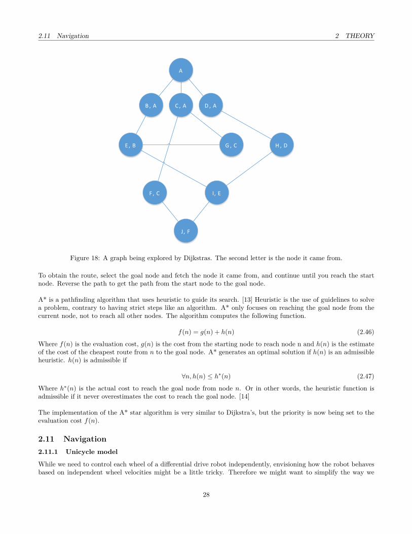
Figure 18: A graph being explored by Dijkstras. The second letter is the node it came from.

To obtain the route, select the goal node and fetch the node it came from, and continue until you reach the startnode. Reverse the path to get the path from the start node to the goal node.

A* is a pathfinding algorithm that uses heuristic to guide its search. [13] Heuristic is the use of guidelines to solvea problem, contrary to having strict steps like an algorithm. A* only focuses on reaching the goal node from thecurrent node, not to reach all other nodes. The algorithm computes the following function.

f(n) = g(n) + h(n) (2.46)

Where f(n) is the evaluation cost, g(n) is the cost from the starting node to reach node n and h(n) is the estimateof the cost of the cheapest route from n to the goal node. A* generates an optimal solution if h(n) is an admissibleheuristic. h(n) is admissible if

∀n, h(n) ≤ h∗(n) (2.47)

Where h∗(n) is the actual cost to reach the goal node from node n. Or in other words, the heuristic function isadmissible if it never overestimates the cost to reach the goal node. [14]

The implementation of the A* star algorithm is very similar to Dijkstra’s, but the priority is now being set to theevaluation cost f(n).

2.11 Navigation2.11.1 Unicycle model

While we need to control each wheel of a differential drive robot independently, envisioning how the robot behavesbased on independent wheel velocities might be a little tricky. Therefore we might want to simplify the way we

28

2.11 Navigation 2 THEORY

design controllers and making it easier to imagine the robot’s movement and thus easier to write control laws ornavigation algorithms. To achieve this we will employ the unicycle model.

The unicycle model let us design our controllers with respect to transitional velocity v and rotational velocity ω ofthe robot frame instead of designing for the rotational velocity of each wheel vl and vr.

The equations that convert motion from the unicycle model to the differential drive are as follows:

vl = 2v − ωL2R (2.48)

vr = 2v + ωL

2R (2.49)

vl is the rotational velocity of the left wheel.

vr is the rotational velocity of the right wheel.

v is the linear velocity of the robot frame.

ω is the rotational velocity of the robot frame.

R is the radius of the wheel.

L is the wheelbase of the robots drive wheels.

These two equations lets us design navigation controllers for v and ω directly. Then use the two parameters asinputs for the unicycle model to calculate independent rotational wheel velocities which are then handed over tothe motor controller.

2.11.2 Behaviours

Rather than program explicit control sequences for the AGV when it enconters different kind of environments andobstacles; in example door algorithm, wall algorithm, moving obstacle algorithm, corridor algorithm, open spacealgorithm etc. We rather want to give the AGV a set of more general behaviors that may be used for dynamicnavigation in varying environments, where the AGV decides what behavior is to be applied given its perception ofenvironment.

Fundamental behaviors to implement:

• Avoid Obstacle

• Go To Goal

• Follow Wall Left

• Follow Wall Right

These behaviors essentially compute vectors to be used by the lower level parts of the navigation system. The AvoidObstacle vector is simply a vector that points in the opposite direction of the obstacle closest to the AGV. The GoTo Goal vector is a vector that points from the AGV’s current position to the goal position. Follow Wall Left andRight are vectors perpendicular to the wall sensed on the respective side of the AGV.

29

2.11 Navigation 2 THEORY

The navigation system decides which one of the vectors to use, or if blending some of the vectors is a more effectivesolution to reach the goal.

As an example let the AGV sense an obstacle between its current position and the goal position, then the navigationsystem may decide to purely use the avoid obstacle vector or a blend of the avoid obstacle and the go to goal vectorto safely and efficiently navigate around the obstacle. This will depend on the proximity of the obstacle detected.

A different example is when the AGV is stuck in a convex obstacle. For instance in a blind corridor or an insidecorner. It will then change its behavior from the current go to goal behavior to follow either the left or right wall.In this manner, the AGV will be able to clear the obstacle by following a wall until some set amount of progresstowards the goal position has been obtained. At this point the navigation system will return to the go to goalbehavior.

GoVector – Most used behavior for direct navigation and concave obstacles:

1. Rotate and align robot with goal vector.

2. Use PID to drive the robot straight along goal vector.

(a) If obstacle within panic range, stop and reverse robot.(b) Else If an obstacle is within avoid range, use obstacle avoidance vector.(c) Else If an obstacle is within blending range, blend goal vector and obstacle avoidance vector.(d) Else go straight to goal.

3. Stop at goal position and rotate to goal pose orientation.

4. If next Goal Vector is available, use this new goal vector and go back to 1.

Follow Wall (Left/Right):

1. Detect line to follow.

2. Calculate vector parallel to wall in direction of travel.

3. Calculate vector perpendicular to wall from AGV reference frame origin.

4. Employ a PID to control the AGV, keep the direction of travel parallel to the wall. And keep the vectorperpendicular to the wall at a set length.

5. If no progress has been made towards goal position, keep following wall.

Roaming – Initial behavior when searching for the required amount of Landmarks to initialize SLAM:

1. Detect largest gap with LIDAR scan by use of vector field histogram.

2. Orient robot towards gap.

3. Drive towards gap 4. Go back to 1.

30

3 DESIGN

3 DesignThe AGV is designed for an indoor environment. The motors and rubber wheels are mounted on an aluminumbase. The outer shell is designed to withstand light impacts, protect against dust and grit collected by the wheelsand of course for the aesthetics.

3.1 Drive system3.2 ChassisInitial design idea for the chassis were a vacuum formed cylinder end cap that encompass all the mechanics andelectronics. However, due to the complexity of first milling a negative form that would then be used in the vacuumforming process, this solution was abandoned. Figure 19 shows the sketch for this design.

Figure 19: First robot design.

Instead a chassis constructed of multiple parts were chosen to stick with the principles of rapid prototyping, keepingthe design modular and easier to modify when needed. The different parts were designed in 3D using SolidWorks.The models were then exported as STL files. These files were in turn imported into CubePro software suite andconverted to a format that could be fed directly into the 3D Systems CubePro printer. Material chosen for thechassis is ABS plastic due to its availability and sufficient strength during testing for the task at hand. Final designcan be seen in figure 20.

In the front of the AGV is the bumper and the IR modules. This will protect the LIDAR from impacts. As theAGV moves around, the module will also hold three infrared sensor aimed down towards the floor. These will detect

31

3.2 Chassis 3 DESIGN

stairs and other cliff features.

Figure 20: Second robot design.

32

3.3 Remote control 3 DESIGN

Figure 21: Computer generated imagery.

3.3 Remote controlIn certain situations it would be convenient for the operator to have direct control of the AGV’s movement knownas remote control or tele-operation. A Sony DualShock 3 controller were selected for this task. This controller isconnected by USB to the operator’s computer. A LabVIEW VI running on this host computer converts the controlinputs given by the operator to values stored in network shared variables. The real-time VI running on the AGV’smyRIO has access to these variables over WIFI and act according to their values.

33

4 COMPONENTS

4 ComponentsA variety of components are required to solve the SLAM problem. Motor encoders to estimate position and aLIDAR for mapping are the most essential components. There is also a need for a battery, motors, a motor driveand a microcontroller to control and drive the AGV. An assortment of components were already supplied for thisproject which removed the need to design, dimension and acquire robot hardware. However, certain additions weredeemed necessary for successfull and safe navigation.

4.1 DC drive motorThe RB-Dfr-444 is a 12 volt brushed DC motor. It comes preassembled with a metal spur-gear gearbox andintegrated quadrature encoder.

Rated torque at 12V 0.147 NmGear ratio 43.7:1

Encoder resolution at motor shaft 64 CPR (counts per revolution)Encoder resolution at gearbox shaft 2797 CPR

Table 3: Motor specifications.

4.2 DC motor controllerSabertooth 2x25 motor controller has two channels and is rated at a maximum of 25A per channel continuous. Italso offers different modes of controlling it, by traditional RC receiver, 0-5V analog signals for each motor or bysupplying it with a byte (0-255) sent over serial line. The required form of input is selected on a DIP switch on themotor controller. One will observe that the specifications of this motor controller far outperforms the requirementsposed by the AGV discussed in this paper. If the controller had not already been supplied a lower spec and cheapercontroller would have been a better option seen from an efficient design point of view.

4.3 NI myRIOmyRIO is a microcontroller developed by National Instruments based on their RIO architecture. RIO is an acronymfor reconfigurable input/output and is based on four components: a processor, a reconfigurable FPGA, measurementI/O hardware, and LabVIEW. [15] The microcontroller run a real-time version of the Linux operating system.[16]

4.4 LIDARHukoyu URG-04LX is a scanning laser range finder. It has a scan angle of 240 degrees and maximum radius of4000mm. Pitch angle is 0.36 degree (resolution). The sensor outputs a maximum of 683 datapoints per scan at amaximum scan rate of 10Hz. Rated accuracy is ±1% of measurement in the range 1000mm-4000mm, for ranges lessthan 1000mm rated accuracy is ±10mm. The LIDAR scan is read as an array consisting of range with correspondingangle data. This will be useful for obstacle avoidance, mapping and navigation.

4.5 Infrared sensorSharp 2Y0A21 sensor returns an analog voltage representing the range to a detected surface. An LED in the deviceemits infrared light which is reflected by the surface that the device is aimed at, a PSD in the device receivesthis reflected light resulting in an analog voltage being transmitted from the sensor to a connected controller. Anincrease in distance is determined by a drop in voltage. Recommended range for this specific sensor is 10cm to80cm. This will be used for cliff detection, ie. determine if the AGV is about to drive off a staircase or otherplatform.

34

4.6 LiPo battery 4 COMPONENTS

4.6 LiPo batteryA 4-cell 14.8V 5000mAh battery were supplied for the project. Relative to the size of the AGV, this is a large andheavy battery. Seeing that one of the possible uses for the AGV might be to deliver parcels and documents betweenoffices in a large building throughout a full working day of 8 hours, a generous battery capacity is advantageous.

4.7 Voltage regulatorThe LiPo battery supplies a varying voltage to the system in the range between ~15V to ~12V depending on itscharge state. However, not all components have a built in voltage regulator to accept this range. For instance, theHukoyu LIDAR requires an external supply of 800mA at 5V. We also realize that external utilities like lights andcameras might be added to the system to expand its functionality. Therefore, two voltage regulators are used.

Input OutputVR #1 12V - 24V 5V, 2.1AVR #2 22.2V - 12V 12V, 1A

Table 4: Overview of input and output voltage of the voltage regulators.

35

5 PROGRAM

5 ProgramThe software for the AGV is made in LabVIEW in the visual programming language G. G has a flowchart like pro-gramming model and works by connecting wires, that transfer data, between nodes. LabVIEW supports modularitywith the use of "Sub-VI’s" that lets one create custom nodes. The program consists of the following major parts,which will be described in better detail in their respective sub chapters. Motor drive, data acquisition, landmarkextraction, landmark association and mapping.

5.1 SchedulingThe program is structured into an initialization, periodic tasks and an termination module. The initializationmodule takes care of initializing the LIDAR and defining global constants. The termination module takes care ofturning off the LIDAR and stopping the motors. The periodic tasks module contains the main robot logic andhas multiple parallel loops executing at different frequencies. At 100Hz, the task controlling the motor controlleris executed. At 33, 3Hz, the task controlling the navigation system is executed. At 10Hz, the task controlling thelocalization and mapping is executed.

5.2 Motor controlMotor control is accomplished by utilizing two PID controllers, one for each motor. Where the set point for eachPID is the reference rotational velocity for the gearbox output shaft. The process variable is the measured shaftrotational velocity. The PID’s are experimentally tuned during testing to give quick and smooth response to changein reference velocity within the desired working envelope.

The output of each PID is conditioned before being sent as a byte to the motor hardware controller. The sabertoothcontroller offers different modes of signal input in order to control each motor. Among the different modes are analogsignal mode which is the most popular one employing a 0-5 volt signal for each motor. Where 2.5V is stop, 0V isfull reverse and 5V is full forward. During testing, we experienced undesirable behavior in analog mode, when themyRIO controller was started or restarted there would be a short moment where the analog output channels sent a0V signal to the motor controller which caused each motor to jerk violently. This could be circumvented by usinga relay to control power between the sabertooth unit and the battery by activating and disabling the relay fromthe myRIO unit. However the sabretooth offered a mode where a byte could be sent over UART to control eachmotor instead of the traditional analog mode. In this mode, the motors would stay disabled during boot up of themyRIO.

Reference velocity for the gearbox shaft is calculated by the unicycle model to differential drive VI.

36

5.2 Motor control 5 PROGRAM

v

omega

vl

vr

vl = (2*v - omega*L) / (2*R);

vr = (2*v + omega*L) / (2*R);

1 2 3

L

R

vr

vl

omega

v

R

L

UniToDiff.vi

We can simplify the control, navigation and obstacle avoidance algorithms by employing the principles of the Unicycle Model. This will let us design navigation controllers with respect to only two simple to understand variables; Translational velocity (v) and Rotational Velocity (omega)

R:AGV wheel radiusL: AGV wheelbase v: Translational velocity omega: Rotational velocity

vl: Rotational velocity of the left motor. vr: Rotational velocity of the right motor.

Figure 22:

vl (rad/s)

vr (rad/s)

R (m)

0

0,001

100

0

0,001

100

Outputs measured

right wheel (rad/s)left wheel (rad/s)

right encoder countleft encoder countright wheel (m/s)left wheel (m/s)

Figure 23: Inputs and outputs of the motor control VI.

The byte is unsigned and has a range from 0-255, where 0 is stop both motors, 1-127 controls motor 1, 128-255controls motor two.

The measured shaft rotational velocity is acquired from the wheel encoders. The accumulated ticks since lastiteration of the motor control VI is used to calculate the rotational velocity. For increased precision and response,this loop is set to run every 10 millisecond, 100 Hz.

ωm1 = encT icks2πN

∆t (5.1)

ωm1 is the rotational velocity of motor one.

encT icks are encoder ticks since last iteration.

N is the resolution of the encoder with respect to the gearbox output shaft.

37

5.3 Sensor data acquisition 5 PROGRAM

∆t is the time in seconds since last iteration.

In this example VI, we can see the process where the inputs; encoder ticks, wheel radius and time since lastiteration are used to control the motor velocity. The VI also outputs useful measurements to be used elsewhere inthe program; encoder ticks, rotational velocity of the output shaft and linear velocity of the wheel mounted to theoutput shaft. We also see how the PID output is conditioned to a byte ranging from 1-127 to control direction andvelocity of the motor and a midpoint of 64 being the command to stop motor one.

encTicks

Linear Velocity [m/s]

Rotaional Velocity [rad/s]

Ref. vl (rad/s)

Reset Counter

Counter Value

Encoder Left

64

1

127

Characters to Writ

Character Count

UART

PID gains

1000

dt (ms) Loop delay, used to calcute velocities

Encoder counts to radians(x/2797)*2*pi

R (m) Wheel radius

Measurements

Figure 24: Code for controlling a motor.

5.3 Sensor data acquisitionThe Hokuyo URG drivers included with LabVIEW is used to communicate with the device. The initializationfunction is called once, at the beginning of the program. It needs to know which device to initialize with anidentifier specified by the Virtual Instrument Software Architecture (VISA) standard. The VISA format is InterfaceType[board index]::Address::INSTR and in the case of the Hokuyo URG-04LX connected to the USB port on themyRio, it is USB0::0x15D1:. The close function is called once, at the end of the program, and attempts to turn offthe laser before terminating the software connection to the instrument. The data acquisition function takes startpoint and end point in degrees and cluster count as parameters. Cluster count refers to the number of measurementswhich are clustered together. The functions returns a magnitude and direction array which are associated. To fetchthe data from the first measurement for instance, the 0th index of each array needs to be accessed.

38

5.4 Line extraction 5 PROGRAM

Figure 25: LabView code for LIDAR data acquisition.

This will still not allow to interface with the laser scanner through LabVIEW. The USB module on the Linuxoperating system is taking control over the laser scanner when connected to the USB port, preventing LabVIEWfrom accessing it. To fix this, we logged into the Linux filesystem and removed the USB module, preventing it fromtaking control over the laser scanner. [17]

5.4 Line extractionA variety of methods were tried to program a fast and robust line extraction algorithm.

RANSAC is one such algorithm and is explained in 2.8.1 on page 23. Instead of returning extracted lines with theRANSAC algorithm, we return a list of fitted points for the lines. Clustering is then performed on the points forfinding the actual start and end points for the lines. To find gaps, we check the distance between each point andthe next point.

d =√

(x2 − x1)2 + (y2 − y1)2 (5.2)

If the distance is greater than a threshold, extract a line with a start point at the end of the last gap and an endpoint at the gap.

39

5.4 Line extraction 5 PROGRAM

Figure 26: Lines extracted from sample data with the RANSAC algorithm.

Split and merge is an other line extraction algorithm. But it does not have any notion of gaps, so the datapointsneeds to be clustered first. Similar to the implementation of clustering in the RANSAC algorithm, but now we areout after the clustered points. Each cluster of points are passed to the Split and Merge module.The Split and Merge module aims to find the corner points making up the extracted lines. The algorithm outlineis explained in chapter 2.8.2 on page 25. Two SubVI’s are defined in the program, one for split and one for merge.The split SubVI picks the two extreme points and finds the line between them. Then it finds the point which liesthe farthest away from the line using 5.3.

d = |−ax+ y − b|√a2 + 1

(5.3)

Where a is the slope of the line, b is where the line intercepts the y-axis, and x and y is the point. If the distanceis big enough, it performs a split. Then recursively call the split SubVI with the left subset of the split and theninserts the point of split to the list of corner points before it calls the split SubVI on the right subset of the split.The tasks are done in this exact order to ensure that both the corner points will appear in a consecutive order inthe list and that the right subset is selected for recursion. The recursion will end when there is no more subsetsthat can do a split. Now the found line segments are sent into the merge SubVI. This SubVI checks consecutivelines for collinearity and removes the point between them if the are collinear enough, effectively merging the lines.The collinearity is found by checking the angle between the lines using 5.4.

α =∣∣∣∣arctan

(m2 −m1

1 +m1 ·m2

)∣∣∣∣ (5.4)

Where m1 and m2 are the slopes of the two lines. The split and merge module returns a linestrip. A linestrip is alist of vertices defining one or multiple lines connected together at its vertices.

40

5.5 Mapping 5 PROGRAM

Figure 27: Lines extracted from sample data with the split and merge algorithm.

With the simulated data, both RANSAC and Split and Merge gave promising results, as seen in figure 26 andfigure 27. To decide which algorithm we wanted to use we tested the two algorithms with real data from the LIDARand in an real environment. The test is described in 6.7 on page 54.

5.5 MappingFor the robot to communicate what it has learned to the user, a topological map is constructed. The map is beingupdated after each time the line extraction algorithm has found some lines. This means that a single wall will bedrawn multiple times on the same place. The line extraction algorithm finds lines in the robot frame and needs tobe transformed into the global frame to be drawn correctly in the map.

−→lG =

−→lR

[cos θ − sin θsin θ cos θ

]+−→R (5.5)

Where−→lR is a vertex in the robot frame, θ is the robot heading, −→R is the robot position and

−→lG is a vertex in the

global frame.

5.6 Landmark extractionCorners are good distinct landmarks the robot can easily extract from the environment. The only problem is thata typical laser scan will contain corners that are not really corners, but just limits in the range of the LIDAR orwalls concealed by other walls. But because Split and Merge returns linestrips, we can just consider all vertices inthe linestrip except for the first and last as corners.

41

5.7 Data association 5 PROGRAM

Landmark

Robot

Not landmark

Extracted line

Wall outside LIDAR range

Figure 28: How landmarks are selected.

5.7 Data associationThe robot maintains a list of observed landmarks. This list is being updated when new landmarks are observed.But it needs some way to distinguish between new landmarks and earlier observed landmarks. We handle this in arather simple way. For each landmark in the current observation, it goes through all the earlier observed landmarksand updates the closest if it is closer than a given threshold. If the landmark is outside the threshold, it adds it asa new landmark to the list.

5.8 EKF SLAMSLAM will be implemented in LabVIEW for the myRIO using wheel encoders and LIDAR by following this outlineof SLAM discussed earlier in the theory chapter.

42

5.8 EKF SLAM 5 PROGRAM

Data Association

Extracted Landmarks

Position Prediction

Encoder Measurements

Observation Prediction

Estimation

Matched Predictions and Observations

Estimated Pose

Predicted Position

Predicted Landmarks

State Vector(Pose and Map)

Landmark Positions

Robot Pose

YES

SLAM

Estimated Landmark

New Landmark

Prediction Step

Update Step

Sensor Observations

Figure 29: Block diagram illustration of the SLAM process.

In the implementation used in this paper, we will expand the state vector with a landmark identifier for eachlandmark. This identifier will store information about the landmark. Is it a new landmark? Is it re-observed?What type of feature, corner, line, gap etc.?

43

5.8 EKF SLAM 5 PROGRAM

Wy

Wx

ml,y

ml,x

rX

ry

rθ

m1,x

m1,y

m1,s

m2,x

m2,y

m2,s

.

.

.mn,x

mn,y

mn,s

Robot pose

Landmarks

Figure 30: Graphical representation of the state vector used in EKF SLAM

The state vector will be represented by a one column matrix of size 3 + N*3, where N is the number of landmarks.

rX

ry

rθ

m1,x

m1,y

m1,s

m2,x

m2,y

m2,s

.

.

.mn,x

mn,y

mn,s

Robot pose

Landmarks

Prl1 . . . PrlN

Pl1l1 . . . Pl1lN

PlNl1 . . . PlNlN

. . .

. . .

Prr

Pl1r

PlNr

. . .

3 2

3

2

2 2

2

2

State Vector Covariance Matrix

3

3

Figure 31: Dimensions of the state vector and covariance matrix.

44

5.8 EKF SLAM 5 PROGRAM

In the mathscript node, arrays and matrices are indexed differently. An arrays’ first index is 0, but the matrix’s firstindex is however 1. It might be convenient to use matrices for all inputs to the mathscript node in order to avoidindexing confusion. The EKF will be written in a mathscript node as the writer of this code is more familiar withtraditional programming languages like C and C++ rather than the graphical programming language of LabVIEW.The mathscript node offers some degree of compilation feedback errors and warnings by attaching an indicator tothe error output node.

We will implement the prediction step, the update step as well as addition of new landmarks. We begin with theprediction step. The inputs for this step is previous state vector, previous covariance matrix and control input.EKFSLAMprediction(xk−1, Pk−1, uk)

xk = fk−1(xk−1, uk) (5.6)

Pk = Fk−1Pk−1FTk−1 +Gk−1Qk−1G

Tk−1 (5.7)

First we set up our matrices with initial values and build our error matrices according the error models discussedin the theory chapter. Initially the state vector is empty apart from the robot pose.

xk−1 =

000

(5.8)

The covariance matrix is initialized accordingly, there are no landmarks and we are fully certain of our initialposition, thus we get the initial covariance matrix.

Pk−1 = P rrk−1 =

0 0 00 0 00 0 0

(5.9)

With initialization complete, write the recursive part of the EKF SLAM algorithm.

Receiving control input recorded from wheel encoders since last iteration.

uk =[

∆sr∆sl

](5.10)

f(x, y, θ,∆sr,∆sl) =

xyθ

+

∆sr+∆sl

2 cos(θ + ∆sr−∆sl

2b)

∆sr+∆sl

2 sin(θ + ∆sr−∆sl

2b)

∆sr−∆sl

b

(5.11)

We compute the error based on the model in the theory chapter.

Qk−1 = covar(∆sr,∆sl) =[kr|∆sr| 0

0 kl|∆sl|

](5.12)

The Jacobian matrices F of the motion model with respect to robot pose, and G of the motion model with respectto control input are defined directly in the mathscript code.

Fk−1 = ∇pf =

1 0 −∆s sin(θ + ∆θ/2)0 1 ∆s cos(θ + ∆θ/2)0 0 1

(5.13)

Gk−1 = ∇∆rl=

12 cos(θ + ∆θ

2 )− ∆s2b sin(θ + ∆θ

2 ) 12 cos(θ + ∆θ

2 ) + ∆s2b sin(θ + ∆θ

2 )12 sin(θ + ∆θ

2 ) + ∆s2b cos(θ + ∆θ

2 ) 12 sin(θ + ∆θ

2 )− ∆s2b cos(θ + ∆θ

2 )1b − 1

b

(5.14)

∆s = ∆sr + ∆sl2 (5.15)

45

5.8 EKF SLAM 5 PROGRAM

∆θ = ∆sr −∆slb

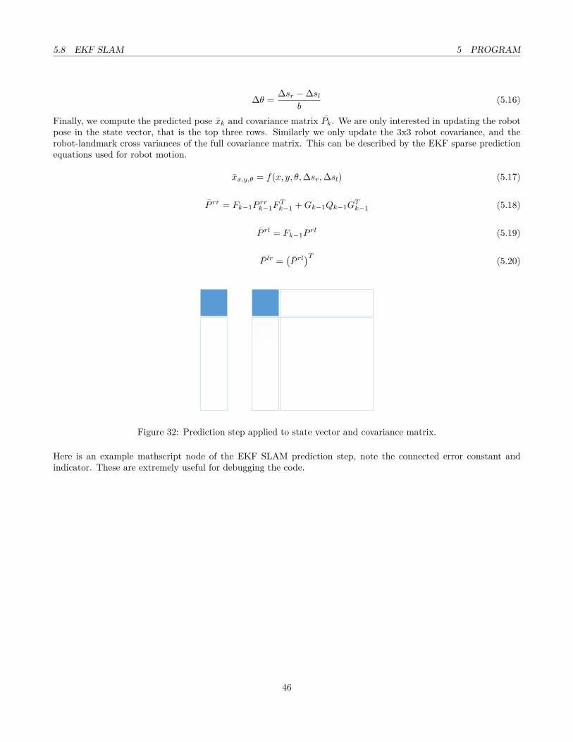
(5.16)

Finally, we compute the predicted pose xk and covariance matrix Pk. We are only interested in updating the robotpose in the state vector, that is the top three rows. Similarly we only update the 3x3 robot covariance, and therobot-landmark cross variances of the full covariance matrix. This can be described by the EKF sparse predictionequations used for robot motion.

xx,y,θ = f(x, y, θ,∆sr,∆sl) (5.17)

P rr = Fk−1Prrk−1F

Tk−1 +Gk−1Qk−1G

Tk−1 (5.18)

P rl = Fk−1Prl (5.19)

P lr =(P rl)T (5.20)

Figure 32: Prediction step applied to state vector and covariance matrix.

Here is an example mathscript node of the EKF SLAM prediction step, note the connected error constant andindicator. These are extremely useful for debugging the code.

46

5.8 EKF SLAM 5 PROGRAM

b = 0.2; % robot wheelsbase [m]deltaSr = u(1,1); % control inputs [m]deltaSl = u(2,1);

dS = (deltaSr+deltaSl) / 2; % delta S [m]dT = (deltaSr-deltaSl) / 2*b; % delta THETA [rad]

% Predict new postionx_new = [x(1,1);x(2,1);x(3,1);] + [dS*cos(x(3,1) + dT/2);

dS*sin(x(3,1) + dT/2); dT ];

% Wrap robot orientation/heading to [-PI,PI]if x_new(3,1) > pix_new(3,1) = x_new(3,1) - 2*pi;

endif x_new(3,1) < -pix_new(3,1) = x_new(3,1) + 2*pi;

end

kr = 0.3; %Error constant right wheelkl = 0.3; % Error constant left wheel

Q = [kr*abs(deltaSr) 0; 0 kl*abs(deltaSl)];

F = [10 -dS*sin(x(3,1) + dT/2); 01 dS*cos(x(3,1) + dT/2); 00 1 ];

G = [0.5*cos(x(3,1)+dT/2)-0.5*(dS/b)*sin(x(3,1)+dT/2) 0.5*cos(x(3,1)+dT/2)+0.5*(dS/b)*sin(x(3,1)+dT/2); 0.5*sin(x(3,1)+dT/2)+0.5*(dS/b)*cos(x(3,1)+dT/2) 0.5*sin(x(3,1)+dT/2)-0.5*(dS/b)*cos(x(3,1)+dT/2);

(1/b) -(1/b) ];

% Predict new covariance matrix using EKF sparse prediction equations P_new(1:3, 1:3) = F*P(1:3,1:3)*F' + G*Q*G'; P_new(1:3, 4:length(P_new)) = F*P_new(1:3, 4:length(P_new)); P_new(4:length(P_new), 1:3) = (P_new(1:3, 4:length(P_new)))';

x = x_new; P = P_new;

1 2 3 4 5 6 7 8 9

10 11 12 13 14 15 16 17 18 19 20 21 2223 24 25 26 27 28 29 30 31 32 33 34 35 36 37 38 39 40 41 42 43

P

x

u

P

x

x

P

u

error out

x2 (Column Vector)

P2

Figure 33: EKF SLAM prediction step, MathScript node.

The update step applies to the full state vector and the full covariance matrix.

47

5.8 EKF SLAM 5 PROGRAM

Figure 34: Update step applied to state vector and covariance matrix.

For each re-observed landmark in zk, compute observation error covariance matrix.

Rk =[krange · zr 0

0 kα

](5.21)

The Jacobian of the observation model.

Hjk =

[−mj,x−xk,x√

q −mj,y−xk,y√q 0 0 0 mj,x−xk,x√

qmj,y−xk,y√

q 0 0mj,y−xk,y

q −mj,x−xk,x

q −1 0 0 −mj,y−xk,y

qmj,x−xk,x

q 0 0

](5.22)

The innovation covariance matrix.

Sk = HkPkHTk +Rk (5.23)

The Kalman gain.

Kk = PkHTk S−1k (5.24)

Apply the Kalman to the state vector.

xk = xk +Kk(zk − hk) (5.25)

Apply the Kalman to the covariance matrix.

Pk = (I −KkHk)Pk (5.26)

Repeat until all re-observed landmarks has been handled.

When handling new landmarks, the state vector is expanded, as is the covariance matrix.

48

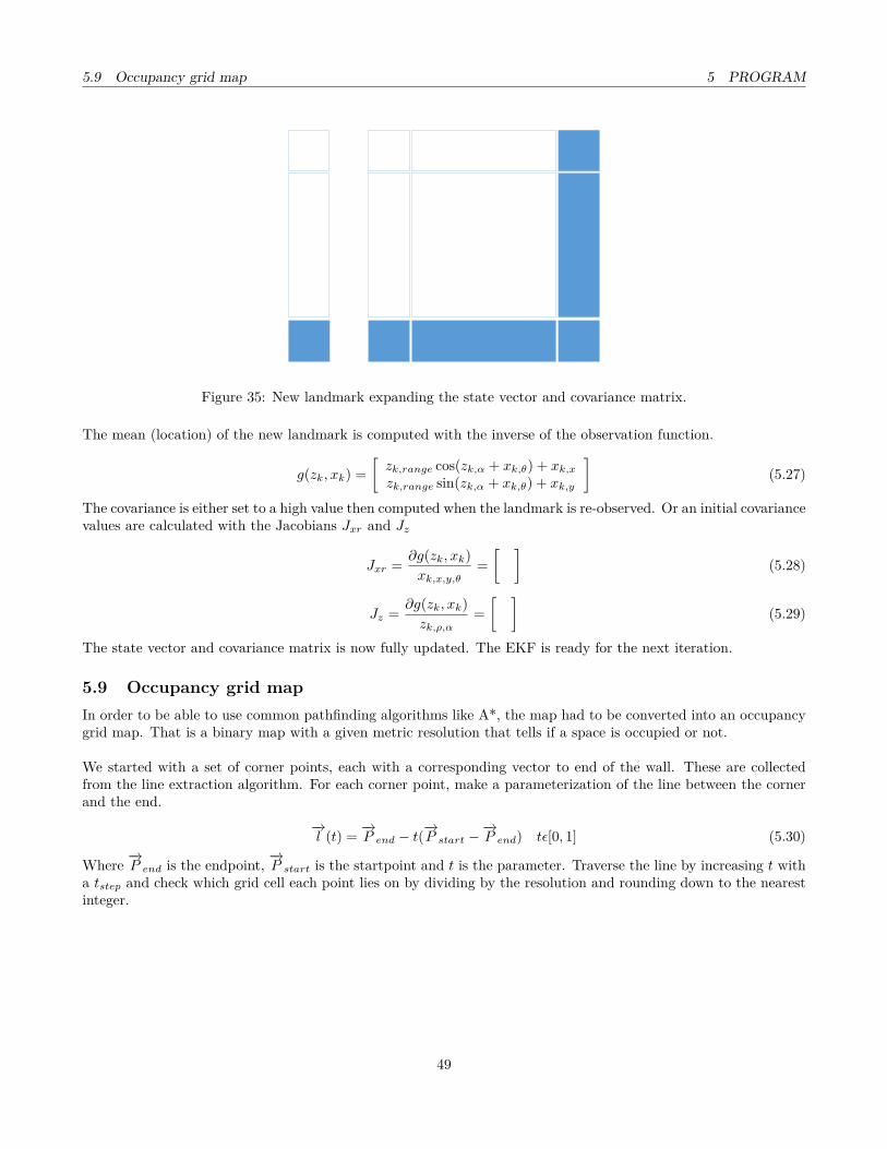
5.9 Occupancy grid map 5 PROGRAM

Figure 35: New landmark expanding the state vector and covariance matrix.

The mean (location) of the new landmark is computed with the inverse of the observation function.

g(zk, xk) =[zk,range cos(zk,α + xk,θ) + xk,xzk,range sin(zk,α + xk,θ) + xk,y

](5.27)

The covariance is either set to a high value then computed when the landmark is re-observed. Or an initial covariancevalues are calculated with the Jacobians Jxr and Jz

Jxr = ∂g(zk, xk)xk,x,y,θ

=[ ]

(5.28)

Jz = ∂g(zk, xk)zk,ρ,α

=[ ]

(5.29)

The state vector and covariance matrix is now fully updated. The EKF is ready for the next iteration.

5.9 Occupancy grid mapIn order to be able to use common pathfinding algorithms like A*, the map had to be converted into an occupancygrid map. That is a binary map with a given metric resolution that tells if a space is occupied or not.

We started with a set of corner points, each with a corresponding vector to end of the wall. These are collectedfrom the line extraction algorithm. For each corner point, make a parameterization of the line between the cornerand the end.

−→l (t) = −→P end − t(

−→P start −

−→P end) tε[0, 1] (5.30)

Where −→P end is the endpoint, −→P start is the startpoint and t is the parameter. Traverse the line by increasing t witha tstep and check which grid cell each point lies on by dividing by the resolution and rounding down to the nearestinteger.

49

5.9 Occupancy grid map 5 PROGRAM

Figure 36: An occupancy grid map represented visually.

The occupancy grid map was not implemented in the robot, but was only simulated on the computer.

50

6 TESTING

6 Testing6.1 White-box testingTo test the software of the robot, white-box testing was used. White-box testing is a method of testing softwarethat tests the internal structure of the program. White-box testing can be applied at the unit and integration level.[18] Unit testing is the testing of individual modules. Does various input yield the expected output? Integrationtesting is the testing of modules in groups. Unit tests are used to ensure that code meets its design and behaves asintended.

6.2 Motor accuracy and performanceA good place to start testing is the performance and accuracy of the motors as this affects how the actuators reactto control inputs. We begin with tuning the PID controllers for each motor. The reference input or set point forthe motor PID controller is the rotational velocity we would like to achieve at the gearbox axle given in radians persecond. Positive rotational direction is counter clockwise when looking straight at the gearbox output shaft. Thefeedback or process variable for the PID is the rotational velocity at the gearbox output shaft. Rotational velocityis computed with data from the motor encoder then accounting for gearbox ratio. We want the motor to achievethe set velocity as quickly as possible while maintaining smooth jitter free acceleration, little to no overshoot fromthe set point and settle at this reference velocity. For safety and peace of mind the AGV is placed on a platformwith the wheels rotating freely without contact with the ground. Keep in mind however that the PID parametersgained from this initial stage will have to be re tuned once the AGV is placed on the ground as the motors thenhave to accelerate the mass of the complete system, not just the wheels spinning freely midair.

Recipe for practical PID tuning:

While this process will not give the perfect PID parameters, it will get you close to it and ensure you get a decentcontroller and hence a responsive system. [19]

1. Set Kp = 1, Ki = 0, Kd = 0.

2. Increase Kp (proportional gain) until the motor achieves steady oscillation when given change in input. Thenset Kp to 80% of this value.

3. Increase Ki (Integral gain) to eliminate the steady state error as quickly as possible. Too high Ki will leadto the motor oscillating around the set point, reduce it.

4. Keep going back and forth between Kp and Ki, making small changes for further improvement to overshoot,performance and stability.

5. If possible introduce some disturbance to the system, in the case of a wheeled robot, simply grab the wheelto restrain its motion the let go of the grip. Observe the response and adjust your controller if an unstableresponse is observed.

6. Experiment with low values of Kd (derivative gain) for increased responsiveness. Often times a PI controllerwill suffice and Kd can be left to 0.

Remember we want stability and reliability first, then performance secondary to that. Below is a result from tuningtwo motors to give a smooth response within the working envelope of this specific differential drive. The boundariesare -6 to 6 radians/second measured on gearbox output shaft.

51

6.3 Straight line test 6 TESTING

7

-7-5

0

5

7

-7-5

0

5

Time

26371614

Left

Right

Velocities

100,000proportional gain (Kc)

0,002integral time (Ti, min)

0,000derivative time (Td, min)

Right wheel PID gains

100,000proportional gain (Kc)

0,002integral time (Ti, min)

0,000derivative time (Td, min)

Left wheel PID gains

-13077

right ticks

13196

left ticks

0

right wheel (rad/s)

0

left wheel (rad/s)

-13077

right encoder count

13196

left encoder count

0

right wheel (m/s)

0

left wheel (m/s)

MotorControl Output

STOP

stop

90,9091

Loop Hz

0

Ref. vl (rad/s)

0

Ref. vr (rad/s)

Figure 37: PID tuning two motors on a differential drive.

6.3 Straight line testWe wanted to test how well the robot managed to drive in a straight line. The purpose of this test is to check ifPID parameters are tuned well and if the physical robot parameters are correct.

6.3.1 Method

A starting point was marked on the floor and an end point was marked 3m away from it. The robot was placed ontop of the starting point and its x-axis was aligned with the end point. The robot was then programmed to drivewhat it believed would be 3m. The distance between the end mark and where the robot actually stopped was thenmeasured.

6.3.2 Test criteria

An error of less than or equal to 10mm for the 3m driven is desired.

6.3.3 Results

Distance (cm) Error (cm)Test 1 302 2Test 2 302.5 2.5Test 3 302.6 2.6Test 4 302.8 2.8Test 5 302.5 2.5

Table 5: Results from the straight line test.

Assuming there is not a systematic error in the encoders, the consistent nature of the error in straight line distancepoints to an error in the measured radius of each wheel, due to the equation.

p = θr (6.1)

The programmed radius of each wheel will have to be increased 302,5−300300 ∼ 1% from its current value.

52

6.4 Rotation test 6 TESTING

6.4 Rotation testThe radius of the wheels were corrected in the preceding step. Another physical parameter of the robot crucialto accurate navigation is the wheelbase, that is the distance between each drive wheels contact point with theunderlying surface.

6.4.1 Method

The wheelbase is initially measured with a ruler. Then the robot is commanded to rotate four full revolutions andthe error in final pose is measured.

6.4.2 Test criteria

Ideally, the error should be as close to zero as possible. However, due to soft pneumatic tires and linear slack ineach gearbox this is obviously not feasible.

6.4.3 Results

Three tests in each rotational direction were performed, for a total of six runs.

Angle (degrees) Error (degrees)Test 1 CW -1430 10Test 2 CW -1428 12Test 3 CW -1428 12Test 4 CCW 1426 -14Test 5 CCW 1428 -12Test 6 CCW 1425 -15

Table 6: Results from rotation test.

Results are consistent and suggest an under estimation the robot wheelbase which leaves it to stop shy of its target inevery test by approximately 12 degrees. The distance of the wheelbase will therefor be increased by 1428−1440

1440 ∼ 1%from its current value.

6.5 Square drive testWe wanted to test how well the robot managed to drive in a rectangle. The purpose of this test is the same as thestraight line test as well as testing how accurate the rotation is.

6.5.1 Method

A plate with the dimensions 1.8m× 0.8m was placed on the floor and the outline was marked with adhesive tape,resulting in a path with the beforementioned dimensions. The robot was placed in one of the corners and wereprogrammed to drive in a rectangle of the same dimensions. The distance error and angle was then measured.

6.5.2 Test criteria

A distance error of less than or equal to 10mm and an angular error of less than 5° is desired.

53

6.6 LIDAR test 6 TESTING

6.5.3 Results

Angle error Distance error (cm)Test 1 12° 27.5Test 2 17° 38.8Test 3 17° 44Test 4 20° 37.2Test 5 14° 40.5

Table 7: Results from the square drive test.

The square drive test shows the robot driving in the pattern of a skewed rectangle and confirms what was indicatedduring the rotation test, again we see a somewhat consistent error over several tests indicating underestimation ofthe robots wheelbase.

6.6 LIDAR testWe trust the specifications provided by Hokuyo to be more accurate then we possibly could measure and test, giventhey probably have a lot better testing setup. But to ensure there is nothing wrong with this specific sensor unit,we wanted to perform a simple test.

6.6.1 Method

The LIDAR was placed 1m from a 1.8m long wall. We then performed a scan to test if the point sensed at θ = 0was 1m from the origin and that the two outermost points were 1.8m apart. The width of the wall is calculatedusing6.2.

d =√r21 + r2

2 − 2r1r2 cos(θ2 − θ1) (6.2)

Where d is the distance between two polar coordinates, r is the magnitude and θ is the direction.

6.6.2 Results

Distance at θ = 0 (mm) The leftmost point (mm) The rightmost point (mm) Width of wall (mm)Test 1 1018 1279∠− 40.547° 1356∠43.125° 1758Test 2 1005 1266∠− 41.953° 1356∠41.016° 1774Test 3 1008 1262∠− 41.25° 1360∠41.719° 1738

Table 8: Results from the LIDAR test.

We observe the results are within the tolerances stated in the data sheet by the manufacturer.

6.7 Line extraction algorithm testTwo algorithms for line extraction has been developed for the project. We want to test which of the implementationsof RANSAC and split and merge performs most accurate and robust.

54

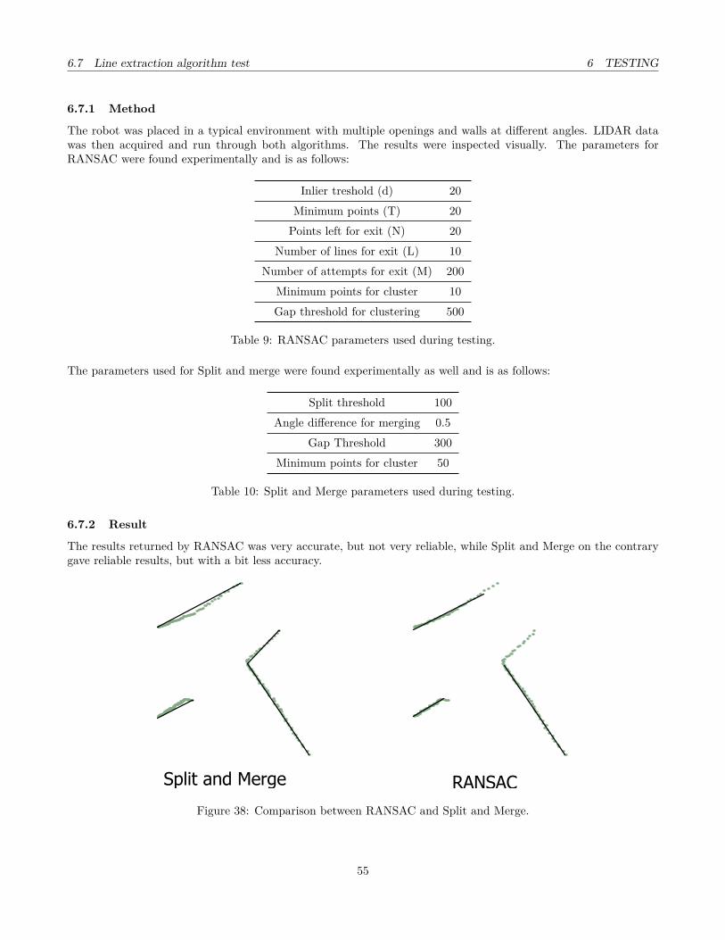
6.7 Line extraction algorithm test 6 TESTING

6.7.1 Method

The robot was placed in a typical environment with multiple openings and walls at different angles. LIDAR datawas then acquired and run through both algorithms. The results were inspected visually. The parameters forRANSAC were found experimentally and is as follows:

Inlier treshold (d) 20Minimum points (T) 20Points left for exit (N) 20

Number of lines for exit (L) 10Number of attempts for exit (M) 200

Minimum points for cluster 10Gap threshold for clustering 500

Table 9: RANSAC parameters used during testing.

The parameters used for Split and merge were found experimentally as well and is as follows:

Split threshold 100Angle difference for merging 0.5

Gap Threshold 300Minimum points for cluster 50

Table 10: Split and Merge parameters used during testing.

6.7.2 Result

The results returned by RANSAC was very accurate, but not very reliable, while Split and Merge on the contrarygave reliable results, but with a bit less accuracy.

RANSACSplit and Merge

Figure 38: Comparison between RANSAC and Split and Merge.

55

6.8 System test 6 TESTING

This could have been caused by not having the optimal parameters. RANSAC has a complexity of S×N×N.Trialswhile Split and Merge has a complexity of N × logN , where N is number of points in the dataset, S is the numberof lines extracted and N.Trials is the number of trials for RANSAC. [20] The split and merge algorithm requiresthe data to be sorted by angle and that is exactly what the LIDAR returns. This concludes that Split and Mergeshould be our obvious choice.

6.8 System testThis is the final test where we test how well the system works together. The robot is placed in a rectangularcoridor that meets itself at the end. It is supposed to drive throught this corridor to see how well it manages tosimultaneous determine own position and map the environment.

6.8.1 Result

Figure 39: Results from testing the robot

The mapping gave promising results, but because of increased uncertainty of in the mapping over time an earliervisited place was placed wrongly on the map. This is the effect of not handling loop closure as explained in 2.9 onpage 26. To prevent this, a loop closure algorithm has to be implemented.

56

7 WRAP-UP

7 Wrap-up7.1 ConclusionThis paper presented a possible real life implementation of online SLAM. Two flavors were presented, one of whichemployed a complementary filter the other approach used the popular EKF approach. While the complementaryfilter is simpler to understand and implement for those less experienced in statistics and probability the EKF onthe other hand does outperform in accuracy when you get it to work.

Much literature were researched in the hunt for the solution to online SLAM EKF, many algorithms studied. Anunfortunate situation that often presented itself was algorithms lacking essential steps, where a simplified version ofSLAM were presented, to simple to be implemented on a real system. Errata in both published articles and highlyregarded literature as well made the algorithms fail when attempts were made to implement them.

To one not familiar in the field of autonomous robots this is the biggest hurdle to overcome and to be able to siftout the good parts from many sources and combine it into a working solution to the SLAM problem is the path onemust travel when tackling this challenge. In this paper a complete algorithm has been presented. It has not howeverbeen successfully implemented on a physical device, due to unrelated hardware issues. Rest assured however, workcontinues.

The beginnings of a navigation system has also been implemented employing among other techniques a vector fieldhistogram and behavior based navigation the robot is able to navigate safely in its environment, avoid static as wellas dynamic obstacles. Way points may also be sent to the robot where it will attempt to find a safe route to thevarious way points in the world. Dealing with convex obstacles remains to be implemented,

A differential drive robot has also been built for this thesis. The drive train and base plate were already given, abody was yet to be designed. This was initially drawn in SolidWorks then the models were exported for 3D printing.

Lastly a series of test cases were written and performed beginning with unit testing ie. encoders to module testingie. drive in a straight line. Full system testing of onlineSLAM was planned but not possible due to reliability andaccuracy issues still to be resolved. Suggestions for further work and improvement will follow.

7.2 Further workAs the project was approaching its end, we still had some ideas that could further improve the performance of therobot.

The occupancy map is currently stored in a grid data structure. To use the occupancy map together with the A*module in LabVIEW, it had to be stored in a 64bit double-precision floating-point format. With a resolution of10mm, a 100m2 map would use 8MB of memory. By using a quadtree structure we could have low resolution wherethe robot has not mapped and high resolution where it has, decreasing the memory used by the map. Empty areasit has visited does not have high resolution. A quadtree is a tree data structure where each node has exactly fourchildren.

Array manipulation is used very much in the code used by the robot. The standard array manipulation functions inLabVIEW makes a copy of the array in memory each time it is being altered. Using the In-place element structure,the operations can be done on the data directly, avoiding making unnecessary copies of the array, thus increasingperformance.

57

7.2 Further work 7 WRAP-UP

Figure 40: Converting an array of cartesian coordinates to polar coordinates using the in-place element.

Landmarks may mistakenly be placed in the wrong place by the robot if the robot pose is determined wrongly.This would further confuse the localization algorithm. By using some sort of algorithm that removes landmarks ifthey seem to not exist, this would be less of a problem. It could also be an idea to

The gear motor that was provided for the project had a good amount of backlash. In addition, the tires were verysoft and flexible. In combination, these two problems made the odometry less accurate. By upgrading the gearmotors and wheels, we predict that the odometry will be improved.

58

REFERENCES REFERENCES

References[1] R. Maxwell. (2013, January) Robotic mapping: Simultaneous localization and mapping (slam). [Online].

Available: https://www.gislounge.com/robotic-mapping-simultaneous-localization-and-mapping-slam/

[2] S. Thrun, W. Burgard, and D. Fox, Probabilistic Robotics. MIT Press, 2005, ch. 5, p. 118.

[3] P. C. Glasser. (2015, May) An introduction to the use of complementary filters for fusion of sensor data.[Online]. Available: http://glassercommunications.com/paul/samples/filters_for_fusion.pdf

[4] H. M. Choset, Principles of robot motion: theory, algorithms, and implementation. MIT press, 2005, ch. 8.

[5] Wikipedia. (2016) Extended kalman filter — Wikipedia, the free encyclopedia. [Online]. Available:https://en.wikipedia.org/wiki/Extended_Kalman_filter

[6] Wolfram MathWorld. (2016, May) Jacobian. [Online]. Available: http://mathworld.wolfram.com/Jacobian.html

[7] G. Robots. (2016) Various techniques for positioning a mobile robot in a space. [Online]. Available:http://www.generationrobots.com/en/content/52-localize-with-a-hokuyo-laser-range-finder

[8] Hokuyo. (2005, October) Scanning laser range finder urg-04lx specifications. [Online]. Available:http://www.hokuyo-aut.jp/02sensor/07scanner/download/pdf/URG-04LX_spec_en.pdf

[9] K. O. Arras. (2009, June) Introduction to mobile robotics. [Online]. Available: http://ais.informatik.uni-freiburg.de/teaching/ss09/robotics/slides/feature_extraction.pdf

[10] B. Williams, M. Cummins, J. Neira, P. Newman, I. Reid, and J. Tardós, “A comparison of loop closingtechniques in monocular slam,” Robotics and Autonomous Systems, vol. 57, no. 12, pp. 1188–1197, 2009.

[11] U. Uttersrud. (2014, November) Datastrukturer for grafer. [Online]. Available: http://www.cs.hioa.no/~ulfu/appolonius/kap11/1/kap111.html#11.1.4

[12] M. Yan. (2014, Januar) Dijkstra’s algorithm. [Online]. Available: http://math.mit.edu/~rothvoss/18.304.3PM/Presentations/1-Melissa.pdf

[13] H. Muñoz-Avila. (2005, October) The a* algorithm. [Online]. Available: http://www.cse.lehigh.edu/~munoz/CSE497/classes/Astar.ppt

[14] Wikipedia. (2015) Admissible heuristic — Wikipedia, the free encyclopedia. [Online]. Available:https://en.wikipedia.org/wiki/Admissible_heuristic

[15] National Instruments. (2014, April) From student to engineer: Preparing future innovators with the nilabview rio architecture. [Online]. Available: http://www.ni.com/white-paper/52093/en/

[16] ——. (2015, Mars) Introduction to ni linux real-time. [Online]. Available: http://www.ni.com/white-paper/14627/en/

[17] X. Smith and N. Asgari. (2014) Robot localisation, navigation and control using national intruments myrio.[Online]. Available: https://wiki.csem.flinders.edu.au/pub/CSEMThesisProjects/ProjectSmit0949/Thesis.pdf

[18] Wikipedia. (2016, April) White-box testing — Wikipedia, the free encyclopedia. [Online]. Available:https://en.wikipedia.org/wiki/White-box_testing

[19] F. Haugen. (2010, April) Tuning of pid controllers. [Online]. Available: http://home.hit.no/~hansha/documents/control/theory/tuning_pid_controller.pdf

[20] N. T. R. S. Viet Nguyen, Agostino Martinelli. (2005) Comparison of line extraction algorithms using 2dlaser rangefinder for indoor mobile robotics. [Online]. Available: http://infoscience.epfl.ch/record/97571/files/nguyen_2005_a_comparison_of.pdf

59

A DIAGRAMS

A DiagramsWirediagram

-

+

PowerSupply

24V

Sabertooth2x25

M2B

B+

B-

M2A

M1B

M1A

0V

5V

S1

S2

DC-Motor

Ma Mb A B V cc Gnd

DC-Motor

Ma Mb A B V cc Gnd

USB

HokyoURG-04LX5V

Gnd

24V->12V V outV in

AdapterGnd Gnd

12V->5V V outV in

AdapterGnd Gnd

D IO15

D IO14

DGND

DGND

D IO13

DGND

D IO12

DGND

D IO11

DGND

UAR T.TX

DGND

UAR T.RX

DGND

AGND

AO1

AO0

+3.3V

D IO10

D IO9

D IO8

D IO7

D IO6

D IO5

D IO4

D IO3

D IO2

D IO1

D IO0

A I3

A I2

A I1

A I0

+5V

5V

DGND

D IO7

D IO6

D IO5

D IO4

D IO3

D IO2

D IO1

D IO0

A I1-

A I1+

A I0+

A I0-

A GND

AO0

AO1

AGND

+15V

-15V

myRio-1900

A

B

C

D IO15

D IO14

DGND

DGND

D IO13

DGND

D IO12

DGND

D IO11

DGND

UAR T.TX

DGND

UAR T.RX

DGND

AGND

AO1

AO0

+3.3V

D IO10

D IO9

D IO8

D IO7

D IO6

D IO5

D IO4

D IO3

D IO2

D IO1

D IO0

A I3

A I2

A I1

A I0

+5V

USB V in Gnd

60

B 3D MODELS

B 3D modelsLeft wheelarc

110

236

Right Wheelarc

236

110

Bumper

210

7043

61

B 3D MODELS

Battery cover147,50

60

Castor wheel

230

10

Instrument panel147,50

95,07

10,22

62

C DATASHEETS

C DatasheetsHokuyo URG-04LX

63

Approved by Checked by Drawn by Designed by

Symbol Pages Date Amendment No

Scanning Laser Range Finder URG-04LX

Specifications

C-42-3389 1/5

Date：2005.10.26

SSSScanningcanningcanningcanning Laser Range Finder Laser Range Finder Laser Range Finder Laser Range Finder URGURGURGURG----04LX04LX04LX04LX

SpecificationsSpecificationsSpecificationsSpecifications

4

MAEDA

Title

Drawing No.

Corrector Amended Reason

SANTOSH MAEJIMA MORI

Changes in cable color

Changes in resolution, revision history of firmware added

Com. Protocol added, revision history of firmware added

Scanning area

Revision history of firmware added x 2

x 1

x 2

x 3

x 5

3,5

4,5

5

5 2008.4.25

2007.4.16

2007.1.18

2006.9.21

2006.6.14

Yamamoto

Maeda

Maeda

Maeda

Maeda

PR-5451

PR-5269

PR-5225

PR-5160

PR-5111

URG-04LX Specification C-42-3389 2/5 Title Drawing No

1. General

URG-04LX is a laser sensor for area scanning. The light source of the sensor is infrared laser of

wavelength 785nm with laser class 1 safety. Scan area is 240º semicircle with maximum radius

4000mm. Pitch angle is 0.36º and sensor outputs the distance measured at every point (683

steps). Laser beam diameter is less than 20mm at 2000mm with maximum divergence 40mm at

4000mm.

Principle of distance measurement is based on calculation of the phase difference, due to which

it is possible to obtain stable measurement with minimum influence from object’s color and

reflectance.

URG-04LX is designed under JISC8201-5-2 and IEC60947-5-2 standards for industrial

applications.

Note Figure 1 shows the detectable area for white Kent sheet (70mm×70mm). Detection distance may vary with size and object. 2. Important Notice This sensor is designed for indoor use only. This sensor is not a safety device/tool This sensor is not for use in military applications Read specifications carefully before use.

Non-detection area: 120º

Power: 5v DC

Interface: RS-232C, USB

Detection Area: 240º

Max. Distance: 4000mm

Figure 1

URG-04LX Specification C-42-3389 3/5 Title Drawing No

3. Specifications

Product name Scanning Laser Range Finder Model URG-04LX

Light source Semiconductor laser diode (λ=785nm), Laser power : less than 0.8mW Laser safety Class 1 (IEC60825-1)

Power voltage 5VDC ±5% Power consumption 500mA or less (Start-up current 800mA)

Detection 60 mm ~ 4,095 mm (Guaranteed accuracy distance) 20mm ~ 5,600mm (Distance)*

Accuracy Distance 20 ~ 1000mm： ±10mm* Distance 1000 ~ 4000mm： ±1% of measurement*

Resolution 1 mm

Scan angle 240°

Angular resolution 0.36°(360°/1024)

Scanning speed 100msec/scan

Interface RS-232C (19.2, 57.6, 115.2 ,500 ,750 kbps) USB Version 2.0 FS mode (12Mbps)

Ambient (Temperature/Humidity)

-10 ~ 50ºC / 85%RH or less (without dew and frost)

Storage temperature -25 ~ 75ºC Ambient light resistance 10000Lx or less

Vibration resistance 1.5mm double amplitude, 10 ~ 55Hz, X, Y and Z direction (2 hours), 98m/s2 55Hz ~ 150Hz in 2 minutes sweep, 1 hour each in X, Y and Z direction

Shock resistance 196 m/s2, 10 times each in X, Y and Z direction

Protective structure Optics : IP64

Case : IP40

Insulation 10MΩ for DC 500Vmegger

Weight Approx. 160 g Casing Polycarbonate

Dimension (W×D×H) 50×50×70mm (Refer to design sheet No. C-40-3362)

*Under standard test conditions with white Kent sheet 70mm×70mm

4. Quality reference value

Operating vibration resistance 19.6m/s2, 10Hz ~ 150Hz with 2 minutes sweep, 0.5 hours each in X, Y and Z direction

Operating impact resistance 49 m/s2, 10 times each in X, Y and Z direction

Angular speed 360 deg/s

Angular acceleration π/2 rad/s2

Lifespan 5 years (Vary on the operating conditions)

Noise level 25db or less (at 300mm)

FDA This product complies with 21 CFR parts 1040.10 and 1040.11. (Registration Number 0521258)

URG-04LX Specification C-42-3389 4/5 Title Drawing No

5. Interface

CN1 (8 Pins) URG-04LX Lead Color 1 N.C. RED

2 N.C. WHITE

3 OUTPUT (SYNCHRONOUS) BLACK 4 GND (9pin Dsub 5p) PURPLE

5 RxD (9pin Dsub 3p) YELLOW

6 TxD (9pin Dsub 2p) GREEN

7 0V BLUE 8 DC 5V BROWN

Note GND and 0V are internally connected A standard unit consists of power supply cable and 9-pin D-sub communication connector

CN2 USB-mini (5 Pin)

Cable is not included. Use commercially available compatible unit.

Communication protocol Please refer to the respective document for details on communication protocol a) SCIP 1.0 : C-42-3320A b) SCIP 2.0 : C-42-3320B

1 Sync signal (approx. 12.5 ms) is outputted at each scan. Figure 2 shows the timing of the

sync signal.

Scan Direction

Scan Range

Sync signal time

Approx. 12.5 ms

Approx. 4.2 ms

Approx. 66.7 ms

Figure 2

URG-04LX Specification C-42-3389 5/5 Title Drawing No

6. Output circuit:

7. Additional notes:

This sensor only needs 5VDC as power supply. Excessive power supply could cause damage to the sensor.

Maximum data step is 683 steps. Since the angular resolution is 0.3515625º (360º /1024 steps), angular range is 239.765625º ((683-1)×360/1024).

Angular resolution is configurable by the host. Read communication protocol specification (No C-42-3320) for details.

Scan direction of the sensor is counterclockwise. In RS-232C communication, communication problems could happen if baud rate above 500

Kbps is set. USB driver used is the communication device class (CDC) supported by standard

operating system. Sensor will be treated as COM port under the same utility when connected to the standard operating system.

Plug and play function of the USB driver is not supported. 8. Firmware revision history Firmware version Changes Ver. 2.91a Laser is not radiated and LED will continue to blink until the connection is

established. Ver. 3.1.00 Fixed for SCIP 2.0. Function in ver. 2.91a is disabled. LED indicating the

power supply will turn ON before communication is establish and start laser radiation.

Ver. 3.1.04 Corrections on MD/MS of SCIP

Ver. 3.3.00 HS command is added. Corrections on MD/MS of SCIP 2.0 Enhancement on error handling

100Ω

0.01µ

Transistor (50V,30mA)

OUT

0v

Figure 3