ufo - theuniversalfeynrulesoutput · defined text files that must be parsed and interpreted, has...
TRANSCRIPT

arX
iv:1
108.
2040
v2 [
hep-
ph]
31
Jul 2
012
CP3-11-25, IPHC-PHENO-11-04, IPPP/11/39, DCPT/11/78, MPP-2011-68
UFO - The Universal FeynRules Output
Celine Degrande a, Claude Duhr b, Benjamin Fuks c,David Grellscheid b, Olivier Mattelaer a, Thomas Reiter d
aUniversite catholique de Louvain,Center for particle physics and phenomenology (CP3),
Chemin du cyclotron, 2, B-1348 Louvain-La-Neuve, BelgiumEmail: [email protected], [email protected]
bInstitute for Particle Physics Phenomenology, University of Durham,Durham, DH1 3LE, United Kingdom,
Email: [email protected], [email protected] Pluridisciplinaire Hubert Curien/Departement Recherches Subatomiques,Universite de Strasbourg/CNRS-IN2P3, 23 Rue du Loess, F-67037 Strasbourg,
FranceE-mail address: [email protected]
dMax-Planck-Institut fur Physik,Fohringer Ring 6, 80805 Munchen, Germany
Email: [email protected]
Abstract
We present a new model format for automatized matrix-element generators, the so-called Universal FeynRules Output (UFO). The format is universal in the sense thatit features compatibility with more than one single generator and is designed to beflexible, modular and agnostic of any assumption such as the number of particles orthe color and Lorentz structures appearing in the interaction vertices. Unlike othermodel formats where text files need to be parsed, the information on the model isencoded into a Python module that can easily be linked to other computer codes.We then describe an interface for the Mathematica package FeynRules thatallows for an automatic output of models in the UFO format.
Key words: Model building, model implementation, Feynman rules, Feynmandiagram calculators, Monte Carlo programs.
Preprint submitted to Elsevier 1 August 2012

1 Introduction
Monte Carlo simulations of the physics to be observed at the Large HadronCollider (LHC) at CERN play a central role in the exploration of the elec-troweak scale, both from the experimental point of view of establishing anexcesses over the expected Standard Model (SM) backgrounds as well as fromthe phenomenological point of view by providing possible explanations for theobservations. For this reason, activities in the field of Monte Carlo simula-tions have been rather intense over the last fifteen years, resulting in manyadvances in the field. Automated tree-level matrix-element generators, such asAlpgen [1], Comix [2], CompHep/CalcHep [3,4,5], Helac [6], Herwig[7,8], MadGraph/MadEvent [9,10,11,12,13], Sherpa [14,15], orWhizard[16,17], describing the hard scattering processes where the Beyond the Stan-dard Model (BSM) physics is expected to show up have been developed. Asa consequence, the problem of the automatic generation of tree-level matrixelements for a large class of Lagrangian-based BSM theories is solved, at leastin principle.
Due to the numerous existing BSM theories based on ideas in constant evo-lution, the implementation of these models into Monte Carlo event genera-tors remains a tedious and error-prone task. Feynman rules associated witha given BSM model must be derived and then implemented one at the timeinto the various codes, which often follow their own specific conventions andformats. A first step in the direction of automating this procedure by startingdirectly from the Lagrangian of the model has been made in the context ofthe LanHep package [18] linked to the CompHep and CalcHep programs.Recently, a new efficient framework going beyond this scheme has been de-veloped. It is based on the FeynRules package [19,20,21,22] and proposes ageneral and flexible environment allowing to develop a model, investigate itsphenomenology and eventually confront it to data. Its virtue has been illus-trated in the context of the CompHep/CalcHep, FeynArts/FormCalc[23], MadGraph/MadEvent, Sherpa and Whizard programs, by imple-menting several new physics theories in FeynRules and then passing themto the different tools for a systematic validation procedure. The approach isbased on a modular structure where each node consists in an interface to a ded-icated matrix-element generator. Since the latter have in general hard-codedinformation regarding the supported Lorentz and/or color structures, the in-terfaces check whether a given vertex is compliant with a given matrix-elementgenerator, in which case the vertex is written to file in a format suitable forthe generator. The final output consists then in a set of text files that can beused in a similar way to any other built-in model.
The procedure spelled out above, where communication between FeynRulesand the matrix-element generators proceeds exclusively via a set of well-
2

defined text files that must be parsed and interpreted, has some serious limita-tions. In particular, extending the format to include more general structures,like higher-dimensional operators and/or non-standard color structures, is dif-ficult to incorporate into a static text-based format. In this paper we presenta new format, dubbed the Universal FeynRules Output or the UFO, formodel files that goes beyond existing formats in various ways. The formatis completely generic and, unlike existing formats, it does not make any a
priori assumptions on the structures that can appear in a model. The aimis to provide a flexible format, where all the information about a model isrepresented in an abstract form that can easily be accessed by other tools.The information on the particles, parameters and vertices of the model arestored in a set of Python objects, each of them being associated with a listof attributes related to their properties. This way of representing the modelinformation has some benefits over the more traditional plain text table-basedformat, because it allows, e.g., to add a missing piece of information directly asa new attribute to an existing object. As an example, extending a table-basedformat to accommodate higher-point vertices requires to change the formatof the table and to adapt the readers for the table accordingly. In an object-oriented format like the UFO, the same extension is trivial, as the number ofparticles entering a vertex is just an attribute of the vertex, so no extensionof rewriting of the readers is necessary. Presently, the UFO format is alreadyused by the MadGraph version 5 [13] and the GoSam generators [24,25,26],and will be used in a near future by Herwig++.
The paper is organized as follows. In Section 2, we describe the features ofthe UFO format as a stand-alone Python module, while Section 3 addressesthe automation of writing an UFO model through FeynRules. Section 4 isdedicated to the UFO features beyond tree level and in Section 5, we providean example of how to implement a model containing non-trivial Lorentz struc-tures with the help of FeynRules into MadGraph 5. Our conclusions aredrawn in Section 6.
2 The UFO format
Any quantum field theory can be defined by a threefold information,
• a set of particles, defined together with their quantum numbers (spin, elec-tric charge, etc.),• a set of parameters (masses, coupling constants, etc, ...),• a Lagrangian describing the interactions among the different particle species.
However, matrix-element generators do not work, in general, directly withthe Lagrangian, but rather with an explicit set of vertices. In the rest of this
3

section, we assume that we have extracted all the vertices from the Lagrangianof a given model and only restrict ourselves to describing a new generic formatto implement the information on the particles and parameters of the modelalong with the vertices describing the interactions among the particles intomatrix-element generators. The issue of the extraction of the vertices fromthe Lagrangian and their translation into this new format in an automatedfashion via the FeynRules package will be discussed in Section 3.
The Universal FeynRules Output (UFO) allows to translate all the infor-mation about a given particle physics model into a Python module thatcan easily be linked to existing matrix-element generators. While in generaleach generator is following its own format and conventions, the UFO formatgoes beyond this approach in the sense that it is, by definition, not tied toany specific matrix-element generator. More specifically, it saves the modelinformation in an abstract (generator-independent) way in terms of Pythonobjects. An UFO model is hence a standalone Python module, containingready-to-go definitions for all the classes representing particles, parameters,etc., and which can be directly linked to an existing matrix-element generatorwithout any modification or further interfacing.
In this section we give a detailed account on the UFO format, putting specialemphasis on the definition of the different classes useful for designing modelfiles. In general, an UFO model consists of a directory containing a set of textfiles that can be split into two distinct classes,
• Model-independent files:- __init__.py,- object_library.py,- function_library.py,- write_param_card.py,• Model-dependent files:- particles.py,- parameters.py,- vertices.py,- couplings.py,- lorentz.py,- coupling_orders.py.
Since the UFO format is based on the Python language, all files have a .py
extension. The model-independent files are identical for every model and con-tain, among others, the definitions of the classes which the model-dependentobjects (particles, parameters, etc.) are instances of. All those files are pro-vided as self-contained Python modules.
4

2.1 Initialization and structure of the objects and functions
A file named __init__.py inside a directory is standard in the Pythonlanguage and corresponds to a tag for importing complete Python modulesby issuing the Python command
import Directory_Name
where Directory_Name refers to the name of the directory containing the__init__.py file. However, in addition to the possiblity of importing a com-plete UFO model, this file also contains, in the UFO case, links to differentlists of quantities associated with the various objects defined in a model,
• all_particles
• all_vertices
• all_couplings
• all_lorentz
• all_parameters
• all_coupling_orders
• all_functions
These lists allow, e.g., to access the full particle content of a model in an easyway downstream in the code. Moreover, every time that an instance of a classis created in the model, it will be automatically added to the correspondinglist.
An UFO model can be fully implemented with the help of a small numberof basic classes, denoted Particle, Parameter, Vertex, Coupling, Lorentzand CouplingOrder. All of these classes are derived from the mother classUFOBaseClass, defining a set of common methods and attributes accessible inthe same way by each class. The mother class, together with all its children, isdefined in the file object library.py. In particular, each class has methodsto display all the attributes associated to a given instance of the class, aswell as to return or set the values of these attributes. As an example, if P isan instance of the class Particle and if charge is an attribute of this class(see Section 2.2), the charge of the corresponding particle can be accessed inthe standard way by issuing the command P.charge. The complete list ofattributes of the UFOBaseClass class is summarized in Table 1.
The file function library.py is related to the implementation of user-definedfunctions into an UFO module via the special class Function, which translatesfunctions that can be defined within a single Python line (i.e., the so-calledPython ‘lambda’ functions) to other programming languages (such as For-tran or C++). Let us note that this specific type of functions is currentlythe only type of user-defined functions supported by the UFO format. A mem-
5

Table 1: Attributes and methods available to all UFO classes
get all Returns a list of all the attributes of an object.
nice string Returns a string with a representation of an object contain-ing the values associated with each of its attributes.
get This method provides access to the value of an attributeof an object. As an example, if P denotes an instance ofa class with attribute charge, then P.get(’charge’) andP.charge are equivalent means of accessing the value of theattribute charge.
set This method allows one to modify the value of an attributeof an object. As an example, if P denotes an instance ofclass with attribute charge, then P.set(’charge’, 1), orequivalently P.charge = 1, will set the attribute denotedby charge to unity.
Table 1
ber of the class Function contains three mandatory attributes, called name,arguments and expression. While name is a string representing the nameof the function, the attributes arguments and expression correspond to asequence of strings for the names of the variables the function depends uponand a string representing the valid Python expression defining the functionitself. Several functions are by default included into the UFO function library,
• complexconjugate: complex conjugation,• csc: the trigonometric function cosecant,• acsc: the cyclometric function arccosecant,• im: the imaginary part of a complex number,• re: the real part of a complex number,• sec: the trigonometric function secant,• asec: the cyclometric function arcsecant.
These functions consist in a set of common mathematical functions for whichthe standard Python module cmath is insufficient or unpractical. As an ex-ample, the cosecant function csc (not included in the cmath library) is im-plemented within the UFO module as an instance of the aforementioned classFunction via
csc = Function(name = ’csc’,
arguments = (’z’,),
expression = ’1./cmath.sin(z)’)
6

2.2 Implementation of the particle content of a model
In the UFO format, all particles are instances of the class Particle defined inthe file particles.py. Even if the Lagrangian of a model is in general moreeasily written in terms gauge eigenstates, matrix-element generators usuallywork at the level of mass eigenstates. Hence only mass eigenstates should bedefined in the particles.py file.
The definition of a particle might read, for, e.g., a top quark, as
t = Particle( pdg_code = 6,
name = ’t’,
antiname = ’t~’,
spin = 2,
color = 3,
mass = Param.MT,
width = Param.WT,
texname = ’t’,
antitexname = ’\\bar{t}’,
charge = 2/3,
line = ’straight’,
LeptonNumber = 0
)
The class Particle has various attributes that are summarized in Table 2. Inthe following we content ourselves to highlight only the most important points.First, note that, apart from a set of mandatory arguments (all attributes butthe last two in the example above), the Particle class can be given an arbi-trary number of optional attributes (the line and LeptonNumber attributes inthe example). There are three predefined optional attributes, which are sum-marized in Table 2. Every additional optional attribute must be an integerrepresenting additional model-dependent additive quantum numbers (as theattribute LeptonNumber in the example). The only exceptions regarding thetreatment of the quantum numbers concern the electric charge and color rep-resentation, which are always mandatory and stored in the attributes chargeand color.
A particle object is identified through its name, a string stored in the name
attribute. In a similar fashion, the attribute antiname is a string representingthe name of the corresponding antiparticle. Note that self-conjugate particles,i.e., particles that are their own antiparticles, are identified by having identi-cal name and antiname attributes (i.e., even for self-conjugate particles, theantiname attribute must be defined). The transformation properties of theparticle under the Lorentz group and the QCD and electromagnetic gauge
7

groups are specified through the spin, color and charge attributes. Each ofthese attributes takes an integer value:
• spin: the possible values are 2s+ 1, where s is the spin of the particle. Forthe moment only s ≤ 2 is supported. By convention, the value −1 is usedfor ghost fields.• color: the possible values are 1, ±3, ±6 and 8, corresponding to singlets,(anti)triplets, (anti)sextets and octets.• charge: any rational number, representing the electric charge of the particle.
Inside matrix-element generators, particles are often identified through aninteger number referring to the Particle Data Group (PDG) numbering scheme[27]. This code is stored in the pdg code attribute, which can be set to anyinteger value, even though it is highly recommended to follow the existingconventions whenever possible. Finally, masses and widths are encoded in themass and width attributes. They refer to the corresponding instances of theParameter class defined in the file parameters.py (see Section 2.3). Therefore,at the beginning of the particles.py file, the Parameter objects are importedvia the Python instruction
import parameters as Param
In the previous example we have only instantiated the object representing thetop quark. However, since the top quark is not a self-conjugate particle, westill need to implement an object representing the top antiquark. We couldproceed in a similar way as in the example above, but the Particle class has abuilt-in method, denoted anti(), instantiating the antiparticle object directlyfrom the corresponding particle object. In the example of the top quark, theinstruction
t__tilde__ = t.anti()
instantiates a Particle object called t__tilde__ which is identical to theobject t previously defined, but with the attributes name (texname) andantiname (antitexname) interchanged. In addition, all the quantum numbers,including the electric charge (charge) and the color representation (color),are set to opposite values.
2.3 Implementation of the parameters of a model
Parameters of a model, like masses, coupling constants, etc., are defined inan UFO model as instances of the Parameter class (itself defined in the fileobject library.py) in the file parameters.py. All the parameters used ina model implementation are either external (or equivalently independent) pa-
8

Table 2: Attributes of the particle class
pdg code An integer corresponding the identification number relatedto the PDG numbering scheme [27].
name A string specifying the name of the particle.
antiname A string specifying the name of the antiparticle. If the par-ticle is self-conjugate, antiname must be identical to name.
spin An integer corresponding to the spin of the particle in theform 2s + 1. By convention, the spin of a ghost field (anti-commuting scalar field) is -1.
color An integer corresponding to the dimension of the color rep-resentation of the particle (1,±3,±6, 8).
mass A Parameter object corresponding to the mass of the par-ticle. If the particle is massless, the value must be set toParam.ZERO.
width A Parameter object corresponding to the width of the parti-cle. If the width is zero, the value must be set to Param.ZERO.
texname A TEX string representing the particle name.
antitexname A TEX string representing the antiparticle name.
charge A rational number equal to the electric charge of the particle.
Optional attributes
goldstone A boolean, tagging a scalar field as a Goldstone boson (true)or not (false). The default value is false.
propagating A boolean, tagging the corresponding particle as auxiliaryand non-propagating (false) field or as a physical field(true). The default value is true.
line A string representing how the propagator of the particleshould be drawn in a Feynman diagram. The possible val-ues are ’dashed’, ’dotted’, ’straight’, ’wavy’, ’curly’,’scurly’,’swavy’ and ’double’. The default value is cho-sen according to the spin and color representation of theparticle.
Table 2
9

rameters or internal (or equivalently dependent) parameters. The user mustprovide as an input the numerical value of the external parameters (e.g.,αs = 0.118), while the internal parameters are related to other (externaland/or internal) parameters via algebraic relations (e.g., gs =
√4παs). Since
internal and external parameters belong to the same generic class Parameter,their declaration is very similar. We will give an example for each case sepa-rately in order to emphasize the main differences and features. The list of allthe possible attributes for the Parameter class is summarized in Table 3.
We start with external parameters. In the UFO format, the external param-eters are all taken to be real and the type attribute of the Parameter classmust be set to the value ’real’. Therefore, complex numbers will have to besplit into their real and imaginary parts. As an example, the declaration ofthe external parameter αs reads
aS = Parameter(name = ’aS’,
nature = ’external’,
type = ’real’,
value = 0.118,
texname = ’\\alpha_s’,
lhablock = ’SMINPUTS’,
lhacode = [ 3 ]
)
The attributes of the Parameter class are all mandatory and contain the nameof the parameter (name), its nature (nature) which is external and the valueof the parameter (value). Since any external parameter is a real number, thevalue must be a real floating point number. The last two arguments, lhablockand lhacode, refer to the Les Houches-like format for the input parameterswhich is followed by the UFO. This is a generalization to any model of theoriginal Supersymmetry Les Houches Accord [28,29]. All the model parametersare grouped into blocks, each line of a block containing a counter (a sequenceof integers) associated with a given parameter name and its correspondingnumerical value. The attribute lhablock of the Parameter object directlyrefers to the name of the block in which the considered parameter is stored,whilst the attribute lhacode is a list of integers referring to the counter.
An additional function related to the Les Houches format is included in the filewrite param card.py. The class ParamCardWriter can be called from withinanother Python module by issuing the instruction
ParamCardWriter(’./param_card.dat’, qnumbers=True)
and outputs a parameter file named param card.dat which contains all theexternal parameters defined in the model, grouped into blocks and countersaccording to their lhablock and lhacode attributes. The first argument in
10

the function above refers to the location of the output file, whereas the secondargument specifies whether or not the QNUMBERS blocks [30] should be includedin the output. In addition, if the second argument is set to True, the full set ofmasses and widths, even if they are dependent parameters, are written to file.In the example of aS presented above, the corresponding entry in the outputfile would read
Block SMINPUTS
3 1.18000e-01 # aS
Let us also note that the file write param card.py can be directly used fromthe command line by issuing the instruction
$> python ./write_param_card.py
As a result, an output file named param card.dat is created and contains thenumerical values of all the external parameters. A snapshot of this parameterfile for a more complete model reads
###################################
## INFORMATION FOR SMINPUTS
###################################
Block SMINPUTS
1 1.325070e+02 # aEWM1
2 1.166390e-05 # Gf
3 1.180000e-01 # aS
###################################
## INFORMATION FOR YUKAWA
###################################
Block YUKAWA
5 4.200000e+00 # ymb
6 1.645000e+02 # ymt
15 1.777000e+00 # ymtau
The definition of internal parameters follows the same lines as for the ex-ternal parameters, with the only differences that the lhablock and lhacode
attributes are not available and that the value argument now contains analgebraic expression relating the parameter to other external or internal pa-rameters. As a simple example, consider the external parameter aS (αs) andthe internal parameter G (gs =
√4παs). The implementation of G reads,
G = Parameter(name = ’G’,
nature = ’internal’,
type = ’real’,
value = ’cmath.sqrt(4 * cmath.pi * aS)’,
11

Table 3: Parameter class attributes
nature A string, either ’external’ or ’internal’, specifyingwhether a given parameter is considered as a dependent orindependent parameter.
name A string, specifying the name of the parameter.
type A string, either ’real’ or ’complex’, specifying whether agiven parameter is a real or a complex number. We remindthat following the UFO synthax, external parameters mustbe real numbers.
value For external parameters, this attribute is a single realfloating-point number. For internal parameters, it consistsof a string representing the analytic expression relating theconsidered parameter to other external and/or internal pa-rameters, following a valid Python syntax.
texname A TEX string representing the parameter name in TEX for-mat.
Attributes specific to external parameters
lhablock A string containing the name of the block which the param-eter is assigned to, following a Les Houches-like format.
lhacode A list of integers giving the position of the considered pa-rameter inside a given lhablock, i.e., the counter associatedwith the parameter, following a Les Houches-like format.
Table 3
texname = ’G’
)
Unlike the case of external parameters, the value attribute is a string rep-resenting a valid algebraic Python expression. Moreover, it is mandatorythat every internal parameter depends only on other parameters which havealready been declared. Returning to our example, the external parameteraS must hence be defined before the internal parameter G inside the fileparameters.py. Note that masses and widths are considered to be param-eters of the model (either internal or external), and must thus be declared assuch in parameters.py.
Let us conclude this section by mentioning that most matrix-element gener-ators have information on the Standard Model input parameters hard-coded.This allows, among others, for a correct handling of the running of the strong
12

coupling constant. Therefore, the Standard Model parameters in an UFOmodel must be correctly identified, following the same notations and con-ventions as for the implementation of a model in FeynRules [20].
2.4 Implementation of the interactions of the model
The vertices corresponding to the interactions included in a model are definedin the file vertices.py using the Vertex class. Let us consider a set of nparticles {φℓiai
i }, with spin indices 1 {ℓi} and color indices {ai}. A generic n-point vertex coupling these fields can be written as a tensor in the color ⊗spin space 2 ,
Va1...an,ℓ1...ℓn(p1, . . . , pn) =∑
i,j
Ca1...ani Gij L
ℓ1...ℓnj (p1, . . . , pn) , (2.1)
where the variables pi denote the particle momenta, Gij the couplings, andthe quantities Ca1...an
i and Lℓ1...ℓnj (p1, . . . , pn) denote tensors in color and spin
space, respectively. Since several vertices may share the same spin and/or colortensors, the latter act as a ‘basis’ for the vertices of the model, the couplingsbeing the ‘coordinates’ in that basis. As an example, the well-known four-gluonvertex,
ig2s fa1a2bf ba3a4 (ηµ1µ4ηµ2µ3 − ηµ1µ3ηµ2µ4)
+ ig2s fa1a3bf ba2a4 (ηµ1µ4ηµ2µ3 − ηµ1µ2ηµ3µ4)
+ ig2s fa1a4bf ba2a3 (ηµ1µ3ηµ2µ4 − ηµ1µ2ηµ3µ4) ,
(2.2)
is written in Eq. (2.1) as
(
fa1a2bf ba3a4 , fa1a3bf ba2a4 , fa1a4bf ba2a3)
×
ig2s 0 0
0 ig2s 0
0 0 ig2s
ηµ1µ4ηµ2µ3 − ηµ1µ3ηµ2µ4
ηµ1µ4ηµ2µ3 − ηµ1µ2ηµ3µ4
ηµ1µ3ηµ2µ4 − ηµ1µ2ηµ3µ4
.(2.3)
The UFO format for vertices mimics exactly this structure. As an example,the implementation of the vertex in Eq. (2.3) into an UFO model reads
V_1 = Vertex(name = ’V_1’,
particles = [ P.G, P.G, P.G, P.G ],
color = [ ’f(1,2,-1)*f(-1,3,4)’,
1 The terminology spin indices refers to both Lorentz and Dirac indices.2 The case of non-strongly interacting particles corresponds to a tensor in colorspace equal to unity.
13

Table 4: Vertex class attributes
name A string specifying the name tag of the vertex.
particles A list of Particle objects containing the set of particles en-tering into the vertex. By convention, all particles are con-sidered outgoing.
color A list of strings representing the color tensors associatedwith the vertex, written as a polynomial combination of theelementary tensors given in Table 5.
lorentz A list of Lorentz objects representing the spin tensors asso-ciated with the vertex.
couplings A list of Coupling objects associated with the decompositionof the vertex in the color ⊗ spin space.
Table 4
’f(1,3,-1)*f(-1,2,4)’,
’f(1,4,-1)*f(-1,2,3)’ ],
lorentz = [ L.VVVV1, L.VVVV2, L.VVVV3 ],
couplings = {(0,0):C.GC_1,
(1,1):C.GC_1,
(2,2):C.GC_1}
)
The Vertex class is probably one of the most important features of the UFOformat, since the vertices associated with a Lagrangian are at the heart ofevery implementation of a BSM model into a matrix-element generator. Itrequires five arguments, which are summarized in Table 4. First, each vertexis identified by an identification tag, its name. Next, the attribute particlescontains the list of all Particle objects entering the considered vertex (byconvention, all particles are considered outgoing). Since these objects are de-fined in the file particles.py, it is necessary to issue at the beginning of thefile vertices.py the command
import particles as P
and a particle object G is now referred to as P.G. The attributes color andlorentz contain two lists with the color and Lorentz tensors associated withthe vertex, i.e., the quantities Ca1...an
i and Lℓ1...ℓnj (p1, . . . , pn) appearing in Eq.
14

Table 5: Elementary color tensors
Trivial tensor (for non-colored particles) 1
Kronecker delta δ2 i1 Identity(1,2)
Fundamental representation matrices (T a1)3 i2 T(1,2,3)
Structure constants fa1a2a3 f(1,2,3)
Symmetric tensor da1a2a3 d(1,2,3)
Fundamental Levi-Civita tensor ǫi1i2i3 Epsilon(1,2,3)
Antifundamental Levi-Civita tensor ǫı1 ı2 ı3 EpsilonBar(1,2,3)
Sextet representation matrices (T a16 )β3
α2T6(1,2,3)
Sextet Clebsch-Gordan coefficient (K6)ı2 3
α1K6(1,2,3)
Antisextet Clebsch-Gordan coefficient (K6)α1
i2j3 K6Bar(1,2,3)
Table 5
(2.1), and are represented inside an UFO module as,
(Ca1a2a3a40 , Ca1a2a3a4
1 , Ca1a2a3a42 ) ↔ [’f(1,2,-1) * f(-1,3,4)’, ... ] ,
(Lµ1µ2µ3µ4
0 , Lµ1µ2µ3µ4
1 , Lµ1µ2µ3µ4
2 ) ↔ [ L.VVVV1, L.VVVV2, L.VVVV3 ] .
Each color tensor is given as a string representing a polynomial combinationof elementary color tensors, whose arguments are integer numbers referring tothe position of the particle in the list particle. If two indices are contracted,they are represented by a negative integer. The set of all the elementary colortensors currently included in the UFO format, together with the correspondingPython syntax, is given in Table 5. Using these conventions, the color tensorsrelated to the four gluon vertex are given by
fa1a2b f ba3a4 ↔ ’f(1,2,-1) * f(-1,3,4)’ ,
fa3a2b f ba2a4 ↔ ’f(1,3,-1) * f(-1,2,4)’ ,
fa1a4b f ba2a3 ↔ ’f(1,4,-1) * f(-1,2,3)’ .
Since the list of color tensors associated with a vertex is a mandatory argumentof the Vertex object, we define the trivial color structure associated with aninteraction among non-colored particles as the color tensor ’1’.
Spin structures such as those appearing in the vertex decompositions in color⊗ spin space are implemented as instances of the class Lorentz. All the struc-tures necessary for the whole model are declared in the lorentz.py file andwe must hence issue at the beginning of the file vertex.py the instruction
15

Table 6: Elementary Lorentz structures
Charge conjugation matrix: Ci1i2 C(1,2)
Epsilon matrix: ǫµ1µ2µ3µ4 Epsilon(1,2,3,4)
Dirac matrices: (γµ1)i2i3 Gamma(1, 2, 3)
Fifth Dirac matrix: (γ5)i1i2 Gamma5(1,2)
(Spinorial) Kronecker delta: δi1i2 Identity(1,2)
Minkowski metric: ηµ1µ2Metric(1,2)
Momentum of the N th particle: pµ1
N P(1,N)
Right-handed chiral projector:(
1+γ52
)
i1i2ProjP(1,2)
Left-handed chiral projector(
1−γ52
)
i1i2ProjM(1,2)
Sigma matrices: (σµ1µ2)i3i4 Sigma(1,2,3,4)
Table 6
import lorentz as L
Hence, the Lorentz objects used in vertex.py, declared in the lorentz.py
Python module, are preceded by the prefix L. As illustrated in the exampleof the four-gluon vertex, the lorentz attribute of the Vertex class containsthe list of the relevant structures. A Lorentz object is instantiated as
FFV1 = Lorentz(name = ’FFV1’,
spins = [ 2, 2, 3 ],
structure = ’Gamma(3,2,1)’)
All attributes are mandatory. While the attribute name is defined in the usualway, the attribute spins contains the list of the values of the spins, written as(2s + 1), of the particles entering the vertex. The last argument, structure,gives the analytical formula of the Lorentz structure as a string. The conven-tions for the spin indices is similar to the convention for the color indices: apositive integer i points to the entry i in the list spins while negative inte-gers are contracted indices. By default, all the Lorentz indices are supposedto be upper indices, and repeated Lorentz indices are contracted using theMinkowski metric. The list of all objects that can be used to define a Lorentzstructure is given in Table 6.
For a given vertex, the Gij quantities appearing in Eq. (2.1) are the ‘coordi-nates’ corresponding to the decomposition of a vertex into the color ⊗ spin
16

basis. The couplings attribute of the Vertex class contains hence a Pythondictionary relating the coordinate (i, j) to a Coupling object, declared in thefile couplings.py,
Gij ↔ (i,j):C.GC 1 ,
By convention, only non-vanishing coordinates Gij are included in this dictio-nary. Moreover, the Coupling objects must be imported at the beginning ofthe vertices.py file through the command
import couplings as C
The declaration of the Coupling objects in the file couplings.py is similar tothe one of internal parameters. Going back to the example of the four-gluonvertex in Eq. (2.3), the coupling GC_1 is defined by
GC_1 = Coupling(name = ’GC_1’,
value = ’complex(0,1)*G**2’,
order = {’QCD’:2}
)
The attribute value is a string giving the algebraic expression of the cou-pling in terms of internal and/or external parameters. The last attribute of aCoupling object, order, is a Python dictionary where the key for each entryis a string and the value a non-negative integer. In the example above, thismeans that the four-gluon vertex is proportional to two powers of the strongcoupling. This feature allows certain matrix-element generators to generateonly subclasses of Feynman diagrams at runtime. This subclass is determinedby giving an upper limit for a given interaction type, specified by the key inthe dictionary order. This concept, together with its implementation into theUFO format, is explained in the next section.
2.5 Controlling various types of couplings in a perturbative expansion
In this section we discuss how to control the different types of expansionparameters that might appear in a perturbative expansion. To illustrate thisconcept, let us consider the production of a weak boson in association with jetsat a hadron collider, e.g., p p→ Z+4 jets. This process is dominated by QCDproduction, while diagrams involving off-shell weak boson exchanges are highlysuppressed. In order to speed up the event generation for this process, it is thusdesirable to focus exclusively on the strong production of the additional fourjets, neglecting all Feynman diagrams with weak boson exchanges. In otherwords, we would like to select the subset of all the diagrams contributing tothe process p p→ Z +4 jets that involve at most one electroweak vertex, i.e.,at most one power of the electromagnetic coupling constant e.
17

This can be achieved using tags that allow to count the number of couplings ofa given type present in a diagram. In the previous section, we have introducedthe order attribute of the Coupling class. As examples, the order of g2swas hence defined as {‘QCD’, 2}, whilst the one of e2 reads {‘QED’:2}. Inthe case of the generation of the Feynman diagrams associated to the p p →Z + 4 jets process, the coupling order feature allows to restrict the number ofcouplings of type QED to be at most one, neglecting in this way the electroweakproduction of any additional jet 3 . For certain models, it can be useful tospecify a default behavior for some types of coupling orders. This can be doneusing the CouplingOrder class, which we describe in the rest of this section.
Coupling orders are instances of the class CouplingOrder and are instantiatedin the file coupling orders.py. As a first simple examples, let us considerthe coupling orders QCD and QED, corresponding to the coupling constants gsand e, respectively. The definitions in coupling orders.py read
QCD = CouplingOrder(name = ‘QCD’,
expansion_order = 99,
hierarchy = 1
)
QED = CouplingOrder(name = ‘QED’,
expansion_order = 99,
hierarchy = 2
)
The class CouplingOrder has two mandatory attributes, apart from the ubiq-uitous name attribute. First, the attribute expansion order is an integer spec-ifying the maximal number of couplings of this type that should be included ina given process. The default value is 99, indicating that any number is allowed.The second attribute, hierarchy, is an integer that allows one to classify dif-ferent types of interactions according to their relative strength. In the aboveexample, we have QCD.hierarchy = 1 and QED.hierarchy = 2, reflecting thefact that g4s is of the same order of magnitude as e2. The CouplingOrder ob-jects then allow certain matrix-element generators to define a default behaviorfor the maximal number of couplings of a given type that can appear in a di-agram, based on the upper bound set by expansion order and the relativestrength among the various couplings.
3 We stress that coupling orders are a property of the matrix-element generators,i.e., the matrix-element generator in question needs to support this feature to useit.
18

3 The FeynRules UFO interface
Even though it is possible to implement a model into the UFO format by hand,this procedure can be a tedious and error-prone task, because all the verticesneed to be entered one at the time. In order to alleviate this problem, we haveimplemented an interface into FeynRules that allows one to export a givenmodel directly in the UFO format. The FeynRules model contains, on theone hand, basic model information (such as the particle content or the pa-rameters of the model) which is implemented as described in Refs. [19,20,22].In particular, a new feature of the FeynRules model files allows to specify thehierarchy between the different types of couplings and the limit up to whichthey should appear in the perturbative expansion (see Section 2.5). Thisis achieved by including the global variables M$InteractionOrderHierarchyand M$InteractionOrderLimit directly into the FeynRules model file 4 .Considering the example of the types of couplings QED and QCD presentedin Section 2.5, the FeynRules model implementation includes then the def-inition
M$InteractionOrderHierarchy = {
{QCD, 1},
{QED, 2}
}
M$InteractionOrderLimit = {
{QCD, 99},
{QED, 99}
}
Note that this new feature is optional for each type of coupling. If a giventype if not represented in one of the two lists, the default values assigned willbe 1 for the hierarchy and 99 for the expansion order.
The FeynRules UFO interface can be called in exactly the same way as allthe other FeynRules interfaces,
WriteUFO[ L1,L2, . . . , options ]
where L1,L2, . . . denote the Lagrangians of the model, and options denotes aset of options supported by the interface. The interface shares all the optionsof the function FeynmanRules[ ], plus some additional options summarizedin Table 7. When this command is issued, FeynRules internally calls thefunction FeynmanRules[ ] to compute all the vertices associated with the
4 InteractionOrder is the FeynRules equivalent to the order attribute of theUFO Coupling object presented in Section 2.4.
19
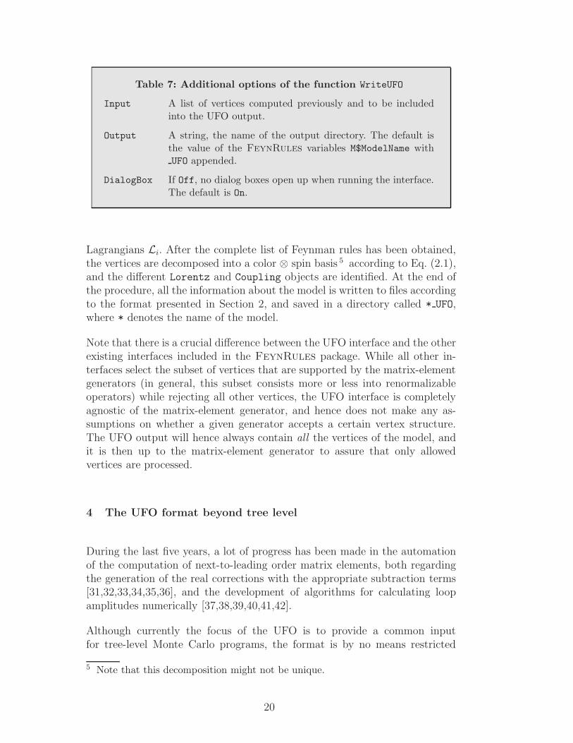
Table 7: Additional options of the function WriteUFO
Input A list of vertices computed previously and to be includedinto the UFO output.
Output A string, the name of the output directory. The default isthe value of the FeynRules variables M$ModelName withUFO appended.
DialogBox If Off, no dialog boxes open up when running the interface.The default is On.
Table 7
Lagrangians Li. After the complete list of Feynman rules has been obtained,the vertices are decomposed into a color ⊗ spin basis 5 according to Eq. (2.1),and the different Lorentz and Coupling objects are identified. At the end ofthe procedure, all the information about the model is written to files accordingto the format presented in Section 2, and saved in a directory called * UFO,where * denotes the name of the model.
Note that there is a crucial difference between the UFO interface and the otherexisting interfaces included in the FeynRules package. While all other in-terfaces select the subset of vertices that are supported by the matrix-elementgenerators (in general, this subset consists more or less into renormalizableoperators) while rejecting all other vertices, the UFO interface is completelyagnostic of the matrix-element generator, and hence does not make any as-sumptions on whether a given generator accepts a certain vertex structure.The UFO output will hence always contain all the vertices of the model, andit is then up to the matrix-element generator to assure that only allowedvertices are processed.
4 The UFO format beyond tree level
During the last five years, a lot of progress has been made in the automationof the computation of next-to-leading order matrix elements, both regardingthe generation of the real corrections with the appropriate subtraction terms[31,32,33,34,35,36], and the development of algorithms for calculating loopamplitudes numerically [37,38,39,40,41,42].
Although currently the focus of the UFO is to provide a common inputfor tree-level Monte Carlo programs, the format is by no means restricted
5 Note that this decomposition might not be unique.
20

to tree-level generators only. Hence, the one-loop matrix-element generatorGoSam [24,25,26] contains an interface to the UFO format, where the infor-mation from the Python module described in Section 2 is translated intoa model definition for the QGraf package [43] together with a Form [44]module substituting the expressions from the Feynman rules. This setup hasbeen successfully applied to simple one-loop calculations in the Minimal Su-persymmetric Standard Model, where the renormalization can still be workedout by hand. For more involved computations, however, one would like toautomate not only the calculation of the matrix elements but also the deriva-tion of the counterterms associated with a given renormalization procedure.Although FeynRules in its current version does not yet support the calcula-tion of renormalization constants and counterterms, we propose in this sectiona generic prescription for their inclusion in the UFO format.
Assuming a multiplicative renormalization prescription, the relation betweenbare and renormalized quantities is given by m0 = Zmmr = (1 + δZm)mr,
where m represents a generic parameter, and by Ψ0 = Z1/2Ψ Ψr = (1+ 1
2δZΨ)Ψr
for the fields. The general case of propagator mixing allows the last equationto take a matrix form. Furthermore, it is assumed that the ultraviolet di-vergences have been regularized dimensionally, the renormalization constantsbeing thus expressed as Laurent series in ǫ = (4−D)/2 where D is the numberof space-time dimensions. Taking into account that the format should not berestricted to one type of perturbative corrections but should be extendable toany αn1
s αn2
EW order of the perturbative expansion, we can make the ansatz
δZi =∞∑
n1,n2=1
αn1
s αn2
EW
(2π)n1+n2
∞∑
p=−∞
z(p)n1,n2ǫp, (4.1)
where, in general, only a small subset of the coefficients z(p)n1,n2is non-zero.
To include the renormalization constants associated with a parameter, wepropose to add an attribute to the Parameter class denoted counterterm.Taking the example of the strong coupling constant introduced in Section 2.3,G, its definition is augmented by
G.counterterm = { (1,0): {-1: ’2./3*NF*TF-11./6*CA’} }
in order to include the QCD one-loop effects on the strong coupling constant.The renormalization constant is represented by a Python dictionary wherethe keys are the pairs (n1, n2) introduced in Eq. (4.1) and the values are theLaurent series in ǫ. The latter are represented by dictionaries with the powersof ǫ as keys and strings representing Python expressions as values. Let usnote that the symbols NF, TF and CA which have been introduced must beeither replaced by their proper values or be defined as model parameters. Formodels containing more than two coupling constants, the pairs (n1, n2) arereplaced by the corresponding n-tuples. Similarly, wave function renormaliza-
21

tion constants 6 are included in the counterterm attribute which is addedto the Particle class. It contains the object δZΨ, implemented following astructure identical to the one described for the Parameter class.
In addition to the renormalization constants, one also needs analytical ex-pressions for the counterterms. In general, they can be described as vertices,starting from two-point vertices for the propagator counterterms, which areincluded in the files ctvertices.py and ctcouplings.py. Analogously, theinitialization file init .py contains, in addition to the lists described in theprevious section, the lists all ctvertices and all ctcouplings. Similarlyto Section 2.4, the file ctvertices.py contains all the counterterm verticesrepresented by objects of the Vertex class, and the related couplings are in-cluded in the file ctcouplings.py. These couplings reflect the nature of therenormalization constants as Laurent expansion in ǫ. Using the generic struc-ture for vertices presented in Eq. (2.1) 7 , we can write a counterterm couplingas
Gij = g(0)ij
∞∑
n1,n2=1
αn1
s αn2
EW
(2π)n1+n2
∞∑
p=−∞
c(p)ij,n1,n2
ǫp . (4.2)
This ansatz allows for some freedom with respect to numeric factors that canbe part of either g
(0)ij or cij,n1,n2
. However, the power of the coupling constants
in g(0)ij must correspond to the one included in the associated tree level vertex.
Hence, the counterterm coupling can be easily declared using the Coupling
class,
GCT_1 = Coupling(name = ’GCT_1’,
value = ’complex(0,1)*G**2’,
counterterm = {(1,0): {-1: G.counterterm}},
order = {’QCD’:2}
)
The prefactor g(0)ij is stored in the value attribute whereas all relative cor-
rections c(p)ij,n1,n2
are mapped to the attribute counterterm, using the samephilosophy as in the case of the classes Parameter and Particle. Finally, theattribute order reflects the interaction order of g
(0)ij and does not take into
account the additional powers of coupling constants coming from the sum overn1 and n2.
The amendments described in this section transmit all information necessaryfor an efficient computation of ultraviolet counterterms by a matrix-elementgenerator. Furthermore, the same approach could be used in order to include
6 Mixing of on-shell particles is assumed to be zero. However, in propagators, mixingis realized through two-point vertices.7 The basis in the color ⊗ spin space associated to a counterterm vertex might bedifferent from the corresponding tree-level one.
22

other counterterm-like objects, such as the rational R2 terms [45,46,47,48] inthe OPP approach [49,50].
5 An example
An UFO model contains the full set of vertices of a model, i.e., all the Lorentzand color structures appearing in all the vertices together with their coeffi-cients. Consequently, it is also suited for models with Lorentz structures thatare not SM-like, a characteristic shared by all models with higher-dimensionaloperators. In the following, we illustrate the UFO format on the example ofthe Strongly Interacting Light Higgs (SILH) model [51]. The SILH model isan effective theory describing the interactions of the Higgs boson consideringit as the Goldstone boson linked to a new strongly interacting sector. Since itis already implemented in FeynRules [20], this model can easily be exportedto the Monte Carlo tools via the corresponding FeynRules interfaces.
The particle content of the SILH model is the same as in the SM. The par-ticularities of the model come solely from the new interactions induced bydimension-six operators involving SM fields. In this short example, we focuson the decay of the Higgs boson H into two W -bosons. The non-SM part ofthe SILH Lagrangian affecting this decay rate reads
LHWWSILH =
cH2f 2
∂µ(
H†H)
∂µ(
H†H)
+icW g
2g2ρf
(
H†σi←→DµH)
(DνWµν)i
+icHW g
16π2f 2(DµH)†σi(DνH)W i
µν (5.1)
where f is the suppression scale for the new operators, g and gρ are the cou-pling constants of the weak and the new strong interaction, respectively, andcH , cW and cHW are free coefficients. In the expression above, we have intro-duced the covariant derivative Dµ (taken in the appropriate representation),the W -boson field strength tensor Wµν , and the Pauli matrices σi. The effec-tive Lagrangian has been obtained after an expansion in 1/f up to O(1/f 2).Hence, the HWW vertex reads now
ig2w
[
v
2
(
1− cHξ
2
)
ηµ2,µ3+ cHW ξ
pµ2
1 pµ3
2 + pµ3
1 pµ2
3 − (p1.p2 + p1.p3) ηµ2,µ3
32π2v
+cW ξ(p2.p2 + p3.p3) ηµ2,µ3
− pµ2
2 pµ3
2 − pµ2
3 pµ3
3
2vg2ρ
]
,(5.2)
where ξ = v2
f2 , v being the vacuum expectation value of the neutral componentof the Higgs doublet, and pi are the momenta of the interacting particles.
23

After an UFO implementation of the model via the corresponding FeynRulesinterface has been obtained, this vertex appears in vertices.py as
V_22 = Vertex(name = ’V_22’,
particles = [ P.W__minus__, P.W__plus__, P.H ],
color = [ ’1’ ],
lorentz = [ L.VVS1, L.VVS5, L.VVS8 ],
couplings = {(0,1):C.GC_56,(0,2):C.GC_59,
(0,0):[ C.GC_30, C.GC_68 ]}).
The color tensor is trivial since all particles are color singlets. On the contrary,the spin structure is more complicated because of the non-trivial tree-levelLorentz structures of Eq.(5.2). As an example, the VVS8 spin tensor is definedin the file lorentz.py as
VVS8 = Lorentz(name = ’VVS8’,
spins = [ 3, 3, 1 ],
structure = ’P(1,3)*P(2,1) + P(1,2)*P(2,3)
- P(-1,1)*P(-1,3)*Metric(1,2)
- P(-1,2)*P(-1,3)*Metric(1,2)’)
The product of VVS8 and GC_59 corresponds to the second term of Eq. (5.2).The coupling order of the coupling is given by NP=1, indicating that it containsone power of ξ. It is important to note that VVS1, the Lorentz structure ofthe first term in Eq.(5.2) is associated with two coefficients, split according totheir coupling order. In particular, GC_30 is the SM part and corresponds tothe order QED=1, while GC_68 is the new physics contribution proportional tocH and of order NP=1. Interferences between SM and new physics operators canbe extracted from the interaction order of the vertex. Indeed, due to our choicefor the ci coefficients, the new physics pieces of the vertex have an interactionorder equal to NP=1 and QED=0. Therefore, the interference is obtained bycomputing the difference between all the contributions (NP=1 QED=1) and thepure SM (NP=0 QED=1) and SILH (NP=1 QED=0) ones.
The Lagrangian of Eq. (5.1) is truncated at order O(1/f 2), or equivalently atorder O(ξ). Computation of matrix elements at higher order in ξ would hencenot be reliable without adding the corresponding terms in the expansion ofthe Lagrangian. For instance, the production of a Higgs-boson pair by weakboson fusion involves a diagram containing two vertices with order NP=1, aspresented in Fig. 1, but also an additional diagram related to the expansionof the Lagrangian at order O(ξ2), which is absent from our SILH model im-plementation. To prevent the user from such issues, the model builder shouldwarn him that O(ξn) amplitudes, with n ≥ 2, cannot be in general computedusing the implemented Lagrangian, and that the NP order should be at mostequal to one. This restriction is easily included in the UFO model through to
24

Fig. 1. Feynman diagram contributing to W+W− → HH at O(ξ2). The shadedboxes represents the O(ξ) part of the HWW vertex in Eq. (5.2).
160 180 200 220 240 260 280 300
0.00
0.01
0.02
0.03
0.04
0.05
0.06
0.07
mH
DG
GSM
UFO+ALOHA+MG5
Analytic
Fig. 2. The relative correction ∆ΓΓSM
≡ ΓSILH−ΓSM
ΓSMto the decay width of the Higgs
boson into two W bosons in the SILH model for gρ = 1, f = 1 TeV, ξ = 0.060623,cH = 4, cW = 2 and cHW = 800. Only the interference terms between SM anddiagrams involving the new operators are taken into account in ΓSILH (see Eq.(6.6) of Ref. [20] and references therein).
the expansion order argument of the CouplingOrder object
NP = CouplingOrder(name = ‘NP’,
expansion_order = 1,
hierarchy = 2
)
The hierarchy argument being set to 2 ensures that the new physics contri-butions are not removed by default in the weak processes.
We choose to validate our UFO model by using the computation tools Mad-Graph version 5 [13], which thanks to the Aloha module [52], allows fora full support of the higher dimensional operators. We have computed theHiggs partial decay width into a W -boson pair, using a very large value forcHW in order to render the associated new physics contribution dominantand to subsequently test the treatment of the higher-dimensional operatorsby MadGraph. Moreover, this contribution is not proportional to the SMresult, contrary to the others. In Fig. 2, we confront the results to hand-madeanalytical calculations and found perfect agreement.
25

6 Conclusion
In this paper, we have presented a new model format for matrix-element gen-erators, the Universal FeynRules Output (UFO) format. While most of thepresent generators have implicit assumptions on the color and/or Lorentzstructures appearing in the different interaction vertices of a given model,the UFO format has been designed to go beyond these constraints, by beingagnostic of any, even unforeseen, restrictions. Indeed, unlike the more tradi-tional table-based model formats (as used by many Monte Carlo codes), theUFO represents all the information about a model terms of abstract Pythonclasses that can accommodate any (reasonable) particle physics model. As anexample, despite the fact that so far only color singlet, triplet, sextet and octetparticles have been implemented into the UFO format, the extension to moreexotic representations of the QCD gauge group is in principle straightforward,without requiring any change to the UFO format itself. A similar change wouldbe very hard to perform in some of the existing table-based model formats.Finally, we emphasize that the format gives a full support to Les Houchesaccord conventions for model parameters and we also illustrate how it couldbe extented in the context of the next-to-leading order tools, including, e.g.,counterterms and the so-called R2 terms. Presently, the UFO format is alreadyused by the MadGraph version 5 and GoSam generators and will be usedin a near future by Herwig++.
Acknowledgments
The authors are grateful to Priscila de Aquino, Neil Christensen, Will Link andto the whole MG5 development team for useful and constructive discussions.ClD and BF are grateful to the CP3 Louvain for the hospitality at variousstages during this project. CeD is a Research Fellow of the ‘Fonds Nationalde la Recherche Scientifique’ (FNRS), Belgium. OM is ‘Chercheur scientifiquelogistique postdoctoral F.R.S-FNRS‘, Belgium. TR is supported by the Hum-boldt Foundation, in the framework of the Sofja Kovaleskaja Award Project“Advanced Mathematical Methods for Particle Physics”, endowed by the Ger-man Federal Ministery of Education and Research. This work was partiallysupported by the Theory-LHC France Initiative, by the Research ExecutiveAgency (REA) of the European Union under the Grant Agreement numberPITN-GA-2010-264564 (LHCPhenoNet), by the Belgian Federal Office for Sci-entific, Technical and Cultural Affairs through the Interuniversity AttractionPoles Program - Belgium Science Policy P6/11-P and by the ISN MadGraphconvention 4.4511.10.
26

References
[1] M. L. Mangano, M. Moretti, F. Piccinini, R. Pittau, A. D. Polosa, ALPGEN, agenerator for hard multiparton processes in hadronic collisions, JHEP 07 (2003)001. arXiv:hep-ph/0206293.
[2] T. Gleisberg, S. Hoche, Comix, a new matrix element generator, JHEP 12 (2008)039. arXiv:0808.3674, doi:10.1088/1126-6708/2008/12/039.
[3] A. Pukhov, et al., CompHEP: A package for evaluation of Feynman diagramsand integration over multi-particle phase space. User’s manual for version 33,arXiv:hep-ph/9908288.
[4] E. Boos, et al., CompHEP 4.4: Automatic computations from Lagrangians toevents, Nucl. Instrum. Meth. A534 (2004) 250–259. arXiv:hep-ph/0403113,doi:10.1016/j.nima.2004.07.096.
[5] A. Pukhov, CalcHEP 3.2: MSSM, structure functions, event generation, batchs,and generation of matrix elements for other packages, arXiv:hep-ph/0412191.
[6] A. Cafarella, C. G. Papadopoulos, M. Worek, Helac-Phegas: a generator forall parton level processes, Comput. Phys. Commun. 180 (2009) 1941–1955.arXiv:0710.2427, doi:10.1016/j.cpc.2009.04.023.
[7] G. Corcella, et al., HERWIG 6: An event generator for hadron emission reactionswith interfering gluons (including supersymmetric processes), JHEP 01 (2001)010. arXiv:hep-ph/0011363.
[8] M. Bahr, S. Gieseke, M. Gigg, D. Grellscheid, K. Hamilton, et al., Herwig++Physics and Manual, Eur.Phys.J. C58 (2008) 639–707. arXiv:0803.0883,doi:10.1140/epjc/s10052-008-0798-9.
[9] T. Stelzer, W. F. Long, Automatic generation of tree level helicity amplitudes,Comput. Phys. Commun. 81 (1994) 357–371. arXiv:hep-ph/9401258,doi:10.1016/0010-4655(94)90084-1.
[10] F. Maltoni, T. Stelzer, MadEvent: Automatic event generation with MadGraph,JHEP 02 (2003) 027. arXiv:hep-ph/0208156.
[11] J. Alwall, et al., MadGraph/MadEvent v4: The New Web Generation, JHEP09 (2007) 028. arXiv:0706.2334.
[12] J. Alwall, et al., New Developments in MadGraph/MadEvent, AIP Conf. Proc.1078 (2009) 84–89. arXiv:0809.2410, doi:10.1063/1.3052056.
[13] J. Alwall, M. Herquet, F. Maltoni, O. Mattelaer, T. Stelzer, MadGraph 5 :Going Beyond, JHEP 1106 (2011) 128. arXiv:1106.0522,doi:10.1007/JHEP06(2011)128.
[14] T. Gleisberg, et al., SHERPA 1.alpha, a proof-of-concept version, JHEP 02(2004) 056. arXiv:hep-ph/0311263.
27

[15] T. Gleisberg, et al., Event generation with SHERPA 1.1, JHEP 02 (2009) 007.arXiv:0811.4622, doi:10.1088/1126-6708/2009/02/007.
[16] M. Moretti, T. Ohl, J. Reuter, O’Mega: An Optimizing matrix elementgenerator, arXiv:hep-ph/0102195.
[17] W. Kilian, T. Ohl, J. Reuter, WHIZARD: Simulating Multi-Particle Processesat LHC and ILC, Eur. Phys. J. C71 (2011) 1742. arXiv:0708.4233,doi:10.1140/epjc/s10052-011-1742-y.
[18] A. Semenov, LanHEP: A package for automatic generation of Feynmanrules from the Lagrangian, Comput. Phys. Commun. 115 (1998) 124–139.doi:10.1016/S0010-4655(98)00143-X.
[19] N. D. Christensen, C. Duhr, FeynRules - Feynman rules made easy,Comput. Phys. Commun. 180 (2009) 1614–1641. arXiv:0806.4194,doi:10.1016/j.cpc.2009.02.018.
[20] N. D. Christensen, P. de Aquino, C. Degrande, C. Duhr, B. Fuks, et al., AComprehensive approach to new physics simulations, Eur.Phys.J. C71 (2011)1541. arXiv:0906.2474, doi:10.1140/epjc/s10052-011-1541-5.
[21] N. D. Christensen, C. Duhr, B. Fuks, J. Reuter, C. Speckner, Exploring thegolden channel for HEIDI models using an interface between WHIZARD andFeynRules, arXiv:1010.3251.
[22] C. Duhr, B. Fuks, A superspace module for the FeynRules package,Comput. Phys. Commun. 182 (2011) 2404–2426. arXiv:1102.4191,doi:10.1016/j.cpc.2011.06.009.
[23] T. Hahn, Generating Feynman diagrams and amplitudes with FeynArts 3,Comput. Phys. Commun. 140 (2001) 418–431. arXiv:hep-ph/0012260,doi:10.1016/S0010-4655(01)00290-9.
[24] P. Mastrolia, G. Ossola, T. Reiter, F. Tramontano, Scattering AMplitudes fromUnitarity-based Reduction Algorithm at the Integrand-level, JHEP 1008 (2010)080. arXiv:1006.0710, doi:10.1007/JHEP08(2010)080.
[25] G. Heinrich, G. Ossola, T. Reiter, F. Tramontano, Tensorial Reconstructionat the Integrand Level, JHEP 1010 (2010) 105. arXiv:1008.2441,doi:10.1007/JHEP10(2010)105.
[26] G. Cullen, N. Greiner, G. Heinrich, G. Luisoni, P. Mastrolia, G. Ossola,T. Reiter, F. Tramontano, Automated One-Loop Calculations with GoSam,arXiv:1111.2034.
[27] K. Nakamura, et al., Review of particle physics, J.Phys.G G37 (2010) 075021.doi:10.1088/0954-3899/37/7A/075021.
[28] P. Z. Skands, B. Allanach, H. Baer, C. Balazs, G. Belanger, et al., SUSYLes Houches accord: Interfacing SUSY spectrum calculators, decay packages,and event generators, JHEP 0407 (2004) 036. arXiv:hep-ph/0311123,doi:10.1088/1126-6708/2004/07/036.
28

[29] B. Allanach, C. Balazs, G. Belanger, M. Bernhardt, F. Boudjema, et al.,SUSY Les Houches Accord 2, Comput.Phys.Commun. 180 (2009) 8–25.arXiv:0801.0045, doi:10.1016/j.cpc.2008.08.004.
[30] J. Alwall, E. Boos, L. Dudko, M. Gigg, M. Herquet, et al., A Les HouchesInterface for BSM Generators, arXiv:0712.3311.
[31] T. Gleisberg, F. Krauss, Automating dipole subtraction for QCD NLOcalculations, Eur. Phys. J. C53 (2008) 501–523. arXiv:0709.2881,doi:10.1140/epjc/s10052-007-0495-0.
[32] M. H. Seymour, C. Tevlin, TeVJet: A general framework for the calculation ofjet observables in NLO QCD, arXiv:0803.2231.
[33] K. Hasegawa, S. Moch, P. Uwer, Automating dipolesubtraction, Nucl. Phys. Proc. Suppl. 183 (2008) 268–273. arXiv:0807.3701,doi:10.1016/j.nuclphysbps.2008.09.115.
[34] R. Frederix, T. Gehrmann, N. Greiner, Automation of the Dipole SubtractionMethod in MadGraph/MadEvent, JHEP 09 (2008) 122. arXiv:0808.2128,doi:10.1088/1126-6708/2008/09/122.
[35] M. Czakon, C. G. Papadopoulos, M. Worek, Polarizing the Dipoles, JHEP 08(2009) 085. arXiv:0905.0883, doi:10.1088/1126-6708/2009/08/085.
[36] R. Frederix, S. Frixione, F. Maltoni, T. Stelzer, Automation of next-to-leadingorder computations in QCD: the FKS subtraction, JHEP 10 (2009) 003.arXiv:0908.4272, doi:10.1088/1126-6708/2009/10/003.
[37] G. Zanderighi, Recent theoretical progress in perturbative QCD,arXiv:0810.3524.
[38] R. K. Ellis, K. Melnikov, G. Zanderighi, Generalized unitarity at work: firstNLO QCD results for hadronic W+ 3jet production, JHEP 04 (2009) 077.arXiv:0901.4101, doi:10.1088/1126-6708/2009/04/077.
[39] C. F. Berger, et al., Precise Predictions for W + 3 Jet Production atHadron Colliders, Phys. Rev. Lett. 102 (2009) 222001. arXiv:0902.2760,doi:10.1103/PhysRevLett.102.222001.
[40] A. van Hameren, C. G. Papadopoulos, R. Pittau, Automated one-loopcalculations: a proof of concept, JHEP 09 (2009) 106. arXiv:0903.4665,doi:10.1088/1126-6708/2009/09/106.
[41] C. F. Berger, et al., Precise Predictions for W + 4 Jet Production at theLarge Hadron Collider, Phys. Rev. Lett. 106 (2011) 092001. arXiv:1009.2338,doi:10.1103/PhysRevLett.106.092001.
[42] V. Hirschi, R. Frederix, S. Frixione, M. V. Garzelli, F. Maltoni,et al., Automation of one-loop QCD corrections, JHEP 1105 (2011) 044.arXiv:1103.0621, doi:10.1007/JHEP05(2011)044.
29

[43] P. Nogueira, Automatic Feynman graph generation, J.Comput.Phys. 105 (1993)279–289. doi:10.1006/jcph.1993.1074.
[44] J. Vermaseren, New features of FORM, arXiv:math-ph/0010025.
[45] G. Ossola, C. G. Papadopoulos, R. Pittau, On the Rational Terms ofthe one-loop amplitudes, JHEP 0805 (2008) 004. arXiv:0802.1876,doi:10.1088/1126-6708/2008/05/004.
[46] P. Draggiotis, M. Garzelli, C. Papadopoulos, R. Pittau, Feynman Rules forthe Rational Part of the QCD 1-loop amplitudes, JHEP 0904 (2009) 072.arXiv:0903.0356, doi:10.1088/1126-6708/2009/04/072.
[47] M. Garzelli, I. Malamos, R. Pittau, Feynman rules for the rational part ofthe Electroweak 1-loop amplitudes, JHEP 1001 (2010) 040. arXiv:0910.3130,doi:10.1007/JHEP01(2010)040,10.1007/JHEP10(2010)097.
[48] M. Garzelli, I. Malamos, R. Pittau, Feynman rules for the rational part of theElectroweak 1-loop amplitudes in the Rxi gauge and in the Unitary gauge,JHEP 1101 (2011) 029. arXiv:1009.4302, doi:10.1007/JHEP01(2011)029.
[49] G. Ossola, C. G. Papadopoulos, R. Pittau, Reducing full one-loop amplitudesto scalar integrals at the integrand level, Nucl.Phys. B763 (2007) 147–169.arXiv:hep-ph/0609007, doi:10.1016/j.nuclphysb.2006.11.012.
[50] G. Ossola, C. G. Papadopoulos, R. Pittau, Numerical evaluation ofsix-photon amplitudes, JHEP 0707 (2007) 085. arXiv:0704.1271,doi:10.1088/1126-6708/2007/07/085.
[51] G. F. Giudice, C. Grojean, A. Pomarol, R. Rattazzi, The Strongly-Interacting Light Higgs, JHEP 06 (2007) 045. arXiv:hep-ph/0703164,doi:10.1088/1126-6708/2007/06/045.
[52] P. de Aquino, W. Link,F. Maltoni, O. Mattelaer, T. Stelzer, ALOHA: Automatic Libraries Of HelicityAmplitudes for Feynman Diagram Computations, Comput.Phys.Commun. 183(2012) 2254–2263. arXiv:1108.2041, doi:10.1016/j.cpc.2012.05.004.
30