University of Calgary

PRISM: University of Calgary's Digital Repository

Graduate Studies The Vault: Electronic Theses and Dissertations

2014-01-29

Development of an Integrated Life Cycle Framework

to Evaluate Emerging Carbon Capture Technologies:

An Albertan Case Study

Ceh, Matthew

Ceh, M. (2014). Development of an Integrated Life Cycle Framework to Evaluate Emerging

Carbon Capture Technologies: An Albertan Case Study (Unpublished master's thesis). University

of Calgary, Calgary, AB. doi:10.11575/PRISM/25667

http://hdl.handle.net/11023/1310

master thesis

University of Calgary graduate students retain copyright ownership and moral rights for their

thesis. You may use this material in any way that is permitted by the Copyright Act or through

licensing that has been assigned to the document. For uses that are not allowable under

copyright legislation or licensing, you are required to seek permission.

Downloaded from PRISM: https://prism.ucalgary.ca

UNIVERSITY OF CALGARY

Development of an Integrated Life Cycle Framework to Evaluate Emerging Carbon

Capture Technologies: An Albertan Case Study

by

Matthew WJ Ceh

A THESIS

SUBMITTED TO THE FACULTY OF GRADUATE STUDIES

IN PARTIAL FULFILMENT OF THE REQUIREMENTS FOR THE

DEGREE OF MASTER OF SCIENCE

DEPARTMENT OF MECHANICAL AND MANUFACTURING ENGINEERING

CALGARY, ALBERTA

DECEMBER, 2013

© Matthew WJ Ceh 2013

ii

Abstract

The critical evaluation of emerging carbon capture and storage (CCS)

technologies is essential to facilitate successful deployment. CCS offers much promise in

reducing the carbon footprint of electricity production, but there are significant cost and

energy penalties associated. Evaluation is complicated by the fact that unique variability

and uncertainty are introduced when evaluating prior to commercialization.

In this thesis, an evaluation of an advanced carbon capture technology is

conducted using a developed framework based on life cycle assessment, energy system

modeling, and life cycle costing. The developed framework can be used to inform the

benchmarking of CCS technologies. The results take into account the significant

upstream impacts from the additional extraction and transport of input fuel required to

compensate for CCS implementation. The development and application of this integrated

life cycle-based tool, will inform current CCS R&D activities and provide better

information to energy policy and investment decision makers.

iii

Acknowledgements

This thesis is the outcome of many interactions with some of the highest calibre

individuals I have ever met. First, I would like to thank my funding sources. Over the

past several years I have benefitted from exceptional guidance and teaching from faculty

in the Department of Mechanical Engineering, and from the Institute for Sustainable

Energy, Environment, and Economy (ISEEE) at the University of Calgary.

I would also like to thank several of the friends and colleagues that I have met

over the years, who have helped me and provided advice on so many issues. And who

have shared in this long journey. I have fond memories of project dates with Hossein

Safaei, Ashley Mercer, Raksha Lakhani, Graeme Marshman, Jessica Abella, and Nic

Levy. All of whom have shared a few ideas and more than a few laughs. I’d like

especially like to thank Ganesh Doluweera for all of his advice, patience, and valuable

time on this project.

I would especially like to thank my thesis supervisor Dr. Joule Bergerson, who

has surely spent countless hours on this work. First, for encouraging me to take LCA at

the masters level, and secondly for encouraging me to join ISEEE in the first place.

Finally, I’d like to thank her for being a wonderful mentor, guide, and role model to

someone who had very little experience in the field of energy and environmental systems.

I am also very fortunate to have Dr. Ron Hugo agree to be my supervisor at such a late

time in this journey. I am very grateful for his support and acceptance of this project.

I am very grateful for my supportive parents, who have been there every step of

the way, even when it meant less time with their grandchildren. Your work ethic, love of

family, and determination in life inspires me.

iv

And finally, to my wife Tobi, and my two sons, Connor and Micah, I will make

up for every single hour I have spent in front of the computer. Tobi, my best friend and

soul mate, I could not have succeeded without your patience, dedication, love and

support. You have taken the load countless times. You have learned more than you ever

cared to learn about engineering. Thank you for letting me pursue this long, long journey,

even through all of the uncertainty.

v

Dedication

To Micah and Connor

vi

Table of Contents

Abstract ................................................................................................................... ii  Acknowledgements ................................................................................................ iii  Dedication ................................................................................................................v  Table of Contents ................................................................................................... vi  List of Tables ......................................................................................................... ix  List of Figures and Illustrations ...............................................................................x  List of Symbols, Abbreviations and Nomenclature ............................................. xiii  

CHAPTER ONE:   Introduction .........................................................................................1  1   Motivation for Study ..................................................................................................1  2   Literature Review of the Evaluation of Advanced CCS Technology ........................4  3   Problem Statement .....................................................................................................6  4   Justification for the Alberta Case Study ....................................................................7  

4.1   Alberta’s Electricity System ..............................................................................8  4.2   Greenhouse Gas Reduction Policies in Canada and Alberta ...........................11  

5   Thesis Overview and Contributions ........................................................................19  

REFERENCES ..................................................................................................................22  

CHAPTER TWO:   Literature Review .............................................................................27  1   Introduction ..............................................................................................................27  2   Literature Review of ESM, LCA, and LCC of CCS Technologies .........................28  3   Literature Review of Uncertainty Assessment Methods .........................................34  4   Literature Review of Existing Energy System Models and Frameworks ................43  

REFERENCES ..................................................................................................................51  

CHAPTER THREE:   Methods ........................................................................................56  1   Introduction ..............................................................................................................56  

1.1   Chapter Overview ............................................................................................56  1.2   Framework Concept Overview ........................................................................57  

2   Integrated Life Cycle Model to Evaluate Electricity Production ............................59  2.1   Introduction ......................................................................................................59  2.2   Electricity Generation Technology Overview .................................................60  

2.2.1   Coal .........................................................................................................61  2.2.2   Natural Gas .............................................................................................63  2.2.3   CCS Technology Overview ....................................................................64  

2.3   Design of Integrated Life Cycle Electricity Production System Model ..........69  2.3.2   Model Design and Relevant Equations ...................................................77  

2.4   Integration with the Uncertainty Assessment Model .......................................86  3   Uncertainty Assessment Model for Evaluating Advanced CCS Technologies .......87  

3.1   Introduction ......................................................................................................87  3.2   Method .............................................................................................................87  

3.2.1   Deterministic Sensitivity Analysis ..........................................................89  

vii

3.2.2   Uncertainty Analysis ...............................................................................91  3.2.3   Stochastic Sensitivity Analysis ...............................................................93  

3.3   Combination with the Integrated Life Cycle Model ......................................101  4   Case Study Formulation .........................................................................................102  

4.1   Alberta’s Future Electric System Pathways ...................................................102  4.2   Scenario Development ...................................................................................103  

4.2.1   Scenario 1 - Base Case ..........................................................................105  4.2.2   Scenario 2 - NGCC ...............................................................................106  4.2.3   Scenario 3 - NGCC with Advanced CCS .............................................106  4.2.4   Scenario 4 - SCPC with CCS ................................................................107  

4.3   Forecast Energy Production ...........................................................................107  4.4   Key Parameter Descriptions and Range Assumptions ...................................108  4.5   Parameter Values and Distribution Characteristics used in the Uncertainty

Assessment Model .........................................................................................115  4.6   Plant and Fuel Specifications and General Economic Assumptions .............116  

REFERENCES ................................................................................................................118  

CHAPTER FOUR:   A Case Study Of CCS Adoption In Alberta’s Electricity Production System ..................................................................................................123  

1   Introduction ............................................................................................................123  1.1   Motivation for Work ......................................................................................123  

2   Case Study Results .................................................................................................124  2.1   Results from the Integrated LC Model ..........................................................124  2.2   Deterministic Sensitivity Analysis .................................................................128  

2.2.1   Contribution Analysis ...........................................................................129  2.2.2   Perturbation Analysis ............................................................................132  

2.3   Uncertainty Analysis ......................................................................................140  2.3.1   Uncertainty Propagation Analysis ........................................................141  2.3.2   Discernibility Analysis ..........................................................................146  

2.4   Stochastic Sensitivity Analysis ......................................................................147  2.4.1   Probability Distribution Scenario Analysis ...........................................147  2.4.2   Probability Distribution Type Sensitivity Analysis ..............................151  2.4.3   Relative Degree of Optimism Analysis ................................................153  2.4.4   Technology Availability and Improvement Analysis ...........................159  2.4.5   Combined Sensitivity and Uncertainty Propagation Analysis ..............163  

3   Conclusions ............................................................................................................168  3.1   Results Summary ...........................................................................................168  3.2   Limitations of the Case Study ........................................................................172  

REFERENCES ................................................................................................................174  

CHAPTER FIVE:   Conclusions .....................................................................................176  1   Introduction ............................................................................................................176  2   Review of Research Questions ..............................................................................178  3   Implications ...........................................................................................................179  

viii

3.1   Implications for Alberta and CCS Implementation .......................................179  3.2   Implications for LCA Studies ........................................................................183  3.3   Implications for Policy ...................................................................................186  

4   Considerations for Future Work ............................................................................187  5   Significance of the Research ..................................................................................190  

REFERENCES ................................................................................................................191  

APPENDIX A: Data Tables .............................................................................................194  

ix

List of Tables

Table 1-1: Alberta Electric Industry’s Share of GHG Reduction Goals [49][52][58] ..... 14  

Table 3-1: Examples of Fossil Fuel Generation Technology Efficiencies and GHG Intensities with and without CCS [2][17] ................................................................. 68  

Table 3-2: Electricity Production Technologies Modeled ................................................ 74  

Table 3-3: Electricity Production Technology Parameters obtained from IECM [2] ....... 75  

Table 3-4: Initial and Final Electricity Energy Production Technology Shares for All Scenarios ................................................................................................................. 105  

Table 4-1: Discernibility Analysis Results for both Environmental Performance and Life Cycle Cost for all Scenarios. ........................................................................... 146  

Table 4-2: Discernibility Analysis Results for Life Cycle Cost for Stable and Unstable NG Prices. ............................................................................................................... 149  

Table 4-3: Discernibility Analysis Results for RDO Analysis for Environmental Performance. ........................................................................................................... 156  

Table 5-1: Power Plant Specifications from IECM v8.0.2 ............................................. 194  

Table 5-2: Parameters used in the Contribution Analysis .............................................. 195  

Table 5-3: Parameter Values used for the Perturbation Analysis ................................... 196  

Table 5-4: Technology Parameter Baseline Distributions .............................................. 197  

Table 5-5: System Parameter Baseline Distributions ..................................................... 197  

x

List of Figures and Illustrations

Figure 1-1: Alberta’s Electricity Energy Share in 2011. .................................................... 8  

Figure 1-2: Alberta’s Generation Capacity Additions by Technology Share from 2000 to 2012. ..................................................................................................................... 10  

Figure 1-3: Alberta’s Climate Change Strategy GHG Emissions Reduction Breakdown. ............................................................................................................... 13  

Figure 2-1: Concept of Framework Use in Advanced CCS Technology Evaluation.. ..... 28  

Figure 3-1: Framework Concept Components.. ................................................................ 57  

Figure 3-2: Technology Schematic for Post-Combustion, Pre-Combustion, and Oxyfuel CCS Technologies. ..................................................................................... 67  

Figure 3-3: Integrated Life Cycle Model Design at the System Level ............................. 71  

Figure 3-4: MATLAB Model Design Concept. ................................................................ 78  

Figure 3-5: Uncertainty Assessment Model and Resulting Output .................................. 89  

Figure 3-6: Discernibility Analysis.. ................................................................................. 93  

Figure 3-7: Probability Distribution Sensitivity Analysis Example using NG Price Stability.. ................................................................................................................... 95  

Figure 3-8: Relative Degree of Optimism Analysis.. ....................................................... 97  

Figure 3-9: Technology Improvement Analysis.. ............................................................. 99  

Figure 3-10: Combined Sensitivity and Uncertainty Propagation Analysis Example.. .. 101  

Figure 3-11: The choices considered for Alberta’s Future Electric System.. ................. 104  

Figure 3-12: Long-term Electricity Energy Forecast for Alberta.. ................................. 108  

Figure 3-13: Range of Values used for the Carbon Capture and Processing Parasitic Power Parameter.. ................................................................................................... 110  

Figure 3-14: Range of Values used for the Capacity Factor for NGCC Plants.. ............ 111  

Figure 3-15: Range of Values used for the Capital Cost of CCS for NGCC Plants.. ..... 111  

Figure 3-16: Henry Hub Gulf Coast Natural Gas Price 1997-2012.. [16] ...................... 113  

Figure 3-17: Range of Values used for the Price of NG.. ............................................... 113  

xi

Figure 3-18: Range of Values used for the Capital Recovery Factor.. ........................... 114  

Figure 3-19: Range of Values used for the Life Cycle Emissions of NG Extraction and Transportation.. ................................................................................................ 115  

Figure 4-1: Deterministic Environmental Performance Results obtained from the Integrated LC Model. .............................................................................................. 125  

Figure 4-2: Deterministic Annual LCOE Results obtained from the Integrated LC Model. ..................................................................................................................... 127  

Figure 4-3: Contribution Results for Environmental Performance in terms of the Cumulative CO2 Emissions.. ................................................................................... 130  

Figure 4-4: Contribution Results for Life Cycle Cost of Scenario 3.. ............................ 131  

Figure 4-5: Perturbation Analysis for Environmental Performance of Scenario 3 – NGCC with CCS.. ................................................................................................... 134  

Figure 4-6: Perturbation Analysis of the difference between environmental results for Scenario 3 and Scenario 4.. ..................................................................................... 135  

Figure 4-7: Perturbation Analysis for the Cost of Scenario 3 – NGCC with CCS. ........ 138  

Figure 4-8: Perturbation Analysis of the Difference Between Cost Results for Scenario 3 and Scenario 4. ...................................................................................... 139  

Figure 4-9: Uncertainty Propagation Analysis for Environmental Performance as the 100-year Cumulative LC Emissions.. ..................................................................... 142  

Figure 4-10: Uncertainty Propagation Analysis for Cost with Stable NG Prices. .......... 144  

Figure 4-11: Uncertainty Propagation Analysis for Cost of CO2 Abatement for Scenario 3.. .............................................................................................................. 145  

Figure 4-12: Chosen Probability Distributions for NG Price.. ....................................... 148  

Figure 4-13: Uncertainty Propagation Analysis for Cost for Unstable NG Prices. ........ 149  

Figure 4-14: Uncertainty Propagation Analysis for Cost of CO2 Abatement for Scenario 3. . ............................................................................................................. 150  

Figure 4-15: Effect of Probability Distribution Type on the Abatement Cost of Scenario 3 using Scenario 2 as a Reference.. .......................................................... 152  

Figure 4-16: Effect of Probability Distribution Type on the Abatement Cost of Scenario 3 using Scenario 2 as a Reference.. .......................................................... 153  

xii

Figure 4-17: Relative Degree of Optimism Analysis Results for Scenario 3 Cost and Environmental Performance.. ................................................................................. 155  

Figure 4-18: Relative Degree of Optimism Analysis Results for Scenario 3 Cost and Environmental Performance. .................................................................................. 157  

Figure 4-19: Relative Degree of Optimism Results for Scenario 3 Abatement Cost for both Reference Cases using Cumulative Population Density.. ............................... 158  

Figure 4-20: Relative Degree of Optimism Results for Scenario 3 with Confidence Level against Scenario 4.. ....................................................................................... 159  

Figure 4-21: Effect of Availability Timing and Improvement in Technology for Scenario 3 Abatement Cost for S1 Reference.. ....................................................... 160  

Figure 4-22: Effect of Availability Timing and Improvement in Technology for Scenario 3 Abatement Cost for S2 Reference. ........................................................ 161  

Figure 4-23: Effect of Availability Timing and Improvement in Technology for Scenario 3 Abatement Costs. .................................................................................. 162  

Figure 4-24: Effect of Availability Timing and Improvement in Technology for Scenario 3 Performance and Cost.. ......................................................................... 163  

Figure 4-25: Combined Sensitivity and Uncertainty Propagation Analysis for all Scenarios.. ............................................................................................................... 165  

Figure 4-26: Combined Sensitivity and Uncertainty Propagation Analysis for S2 and S3. ........................................................................................................................... 166  

Figure 4-27: Combined Sensitivity and Uncertainty Propagation Analysis for S1 and S3. ........................................................................................................................... 167  

Figure 4-28: Combined Sensitivity and Uncertainty Propagation Analysis for S3 and S4. ........................................................................................................................... 167  

xiii

List of Symbols, Abbreviations and Nomenclature

Symbol Definition AESO Alberta Electric Systems Operator AIES Alberta Interconnected Electric System CO2e Carbon dioxide equivalents ESM Energy System Modeling GHG Greenhouse gas GJ Gigajoule Gt Gigatonne IGCC Integrated gasification combined cycle IPCC Intergovernmental Panel on Climate Change ISO International Organization for Standardization kt Kiloton kWh Kilowatt-hour LCA Life Cycle Assessment LCC Life Cycle Costing LHS Latin Hypercube Sampling LTTP Long Term Transmission Plan MCS Monte Carlo Simulation MJ Megajoule MPa Megapascals MWh Megawatt-hour NG Natural gas NGCC Natural gas combined cycle NGSC Natural gas simple cycle NOx Nitrous oxides NPV Net present value O&M Operational and maintenance costs PC Pulverized coal RET Renewable Energy Technologies SCPC Supercritical pulverized coal SGER Specified Gas Emitters Regulation SOx Sulfur oxides TWh Terawatt-hour UCG Underground Coal Gasification USCPC Ultra supercritical pulverized coal

1

CHAPTER ONE: Introduction

1 Motivation for Study

Climate change and its associated mitigation policies and political debate have

placed pressure on electric power systems to manage their greenhouse gas (GHG)

emissions. In 2010, these systems were responsible for 41% of total global GHG

emissions [1]. Many technological options to manage the GHG emissions of electric

power systems exist and have had varying degrees of success in deployment [2].

Renewable energy technologies such as biomass, wind, solar are solutions that are

gaining global momentum. However, deployment has been slower than originally

anticipated due to social, economic, and environmental barriers [3][4]. Nuclear

technologies have a very small GHG emissions footprint but cost of new builds are

uncertain and they are high in perceived risk [5]. The growing global population and its

increasing demand for energy makes it likely that the large supply of fossil fuel energy

will be further exploited [6]. If fossil fuels are to continue as a source of power, new

technologies must be implemented to address the threat of climate change and the

accompanying political pressure.

Technologies to reduce GHG emissions have already been deployed. Efficiency

improvements in fossil energy conversion, such as natural gas based cogeneration of heat

and electricity as well as Natural Gas Combined Cycle (NGCC) technologies have seen

widespread adoption worldwide [7][8]. Cogeneration has shown a recent increase in

Alberta with over 3 gigawatts of cogenerated electricity installed since 2000 [9]. Much of

this new capacity is due to the increased demand for thermal energy (steam) and

2

electricity in the oil sands industry. Coal is the primary fuel for electricity production in

the U.S. (49% coal vs. 22% NG [10]), Canada (14% coal [11] vs. 8% NG [12]) and

Alberta (55% coal vs. 35% NG [13]). Recently, natural gas (NG) has started to displace

coal due to historically low prices of NG and anticipation of incoming GHG regulations

[14][15]. However, even if the trend of switching to NG from coal continues, further

GHG mitigation is required to achieve reductions in emissions that will achieve

International Panel on Climate Change (IPCC) stabilization targets1 to avoid the full

effects climate change [4].

Decarbonization of the power sector through Carbon Capture and Storage (CCS)

is a unique option for reducing emissions in that it can make deep reductions in the power

sector while continuing to make use of cheap and plentiful fossil fuels. Each has the goal

of capturing and storing greater than 90% of the CO2 generated. These CCS technologies

offer much promise in reducing the carbon footprint of electricity production.

Though CCS has the potential to make an impact in GHG emissions reduction,

there are significant barriers to successful deployment. The first involves the cost

associated with CCS (and in particular the cost of capture), which is a significant

deterrent of investment on a large scale. In fact, a study by Herzog has suggested “the

cost of CCS mitigation may be more than is politically acceptable for the next couple of

decades” [17]. A second barrier is the additional fuel required to cover the additional

energy required to operate the CCS system, resulting in increased upstream GHG

emissions from the extraction and processing of the fuel [18]. This means that actual

1 GHG concentrations would need to be stabilized in the range of 445 to 490 ppm CO2eq in the atmosphere to limit the rise in average global temperature to 2C. [16]

3

GHG reductions are less than the intended goal. In addition, the energy penalties

associated with capturing and compressing CO2 result in significant declines in overall

efficiency of the plant [19]. Finally, there are competing societal perception issues with

the use of CCS (i.e., using CCS to reconcile coal use with climate change over the use of

cleaner sources of energy) [20], along with concerns regarding the support for CCS use in

climate change mitigation [21]. Consequently, CCS is currently in use only in small-scale

projects with a total capture rate less than 40 millions of metric tonnes of CO2 per year

[22], where it is required on a much larger scale to be an effective global GHG mitigation

tool.

There has been effort in the research community to assess CCS technologies in

order to provide information for further technology development and deployment. Some

studies have estimated that cost reductions of up to 40% below current technologies are

possible [23]. More advanced technologies that address the above performance and cost

issues can be found in several pilot projects worldwide (e.g., [24]) or are currently at the

lab or bench scale [25]. However, there are uncertainties associated with these advanced

technologies that in turn, increase the variability and uncertainty of the potential

environmental impacts of the technology. For example, there is greater uncertainty

associated with the projected performance (e.g., efficiency impacts) and cost (e.g.,

additional cost of retrofits) of the technology at commercial scale. Additionally,

variability in the way that the technology could ultimately be implemented at commercial

scale (e.g., a CCS capture technology will perform differently if implemented in a coal

power plant vs. a NGCC power plant) is also a consideration. This study addresses the

uncertainty and variability in advanced CCS technologies with a systematic quantitative

4

analysis with an overriding goal of improving the reliability of the results used for

decision-making.

2 Literature Review of the Evaluation of Advanced CCS Technology

Decision-makers in industry require information about the characteristics and

risks associated with emerging technologies to make informed decisions about

investment choices. Those in government require information to make effective policies

that influence and encourage industry to make choices that help to meet GHG targets.

The characteristics (e.g., capture system energy requirements, capital and operating costs,

and capture rates) and risks (e.g., economic and environmental) associated with emerging

CCS technologies are valuable information for these decision makers, and can be

estimated using several analytical tools. Three examples are Energy System Modeling

(ESM), Life Cycle Costing (LCC), and Life Cycle Assessment (LCA). ESM (e.g., [26-

28]) is defined as representing an “integrated set of technical and economic activities

operating within a complex societal framework” [29]. LCC (e.g., [26][30]) is a method

to evaluate the total costs of ownership of a technology or process, including the costs of

building, operation, disposal, and externalities such as environmental costs [31]. LCA

(e.g., [32-34]) is a tool to evaluate the environmental impacts of a product or process

from the extraction of resources through to the disposal of unwanted residuals [35]. These

tools can help to uncover the trade-offs (e.g., capturing CO2 at the expense of efficiency

and additional cost) that must be faced to achieve a stated set of objectives (e.g.,

emissions reduction targets). Critical evaluation of these trade-offs is essential to

facilitate successful deployment and inform decision makers of the potential implications

of their use. The benefits of engaging in LCAs are that they can help to avoid unintended

5

consequences (e.g., avoid creating new or compounding existing problems when actually

deployed), prioritize lab scale research (e.g., identify specific processes and products

where the biggest impacts occur), and better understand the timeframe and performance

level that is required to see these technologies play an important role in achieving

emissions reduction targets. However, the analysis of these advanced CCS technologies

is complicated by the fact that unique variability and uncertainty is introduced (i.e.,

through technology parameters, economic environment, and deployment horizons) when

scaling up for evaluation.

Recent analyses of CCS technologies have included various methods and

approaches for uncertainty assessment (i.e., defining sources of and quantifying

uncertainty). These studies are important in that they reveal case specific and/or detailed

comparative results, and provide detailed techno-economic assessments of potential game

changing technologies. However, as suggested by Rubin et al. [25], they may present

overly optimistic projections of future cost reductions by not fully exploring the effects of

uncertainty. Most include limited assessment of the inherent uncertainties of these

emerging technologies or are limited in scope to individual plants. For example,

deterministic analyses with some discussion of uncertainty are used in some studies (e.g.,

[34][36]). However, previous studies lack quantification of uncertainty, which has

resulted in a lack of understanding about the probability of uncertain results actually

occurring. Others use various sensitivity analyses to explore the sources of uncertainty

(e.g., [32][33][37-39]), and some have used scenario analysis (e.g., [28]) to explore the

effects of uncertainty in alternate choices on outcomes. However, they do not consider

the propagation of parameter uncertainty in models used in the evaluation and therefore

6

do not quantify the uncertainty in the results or the effects this would have in the

outcomes. Others have gone further, using uncertainty propagation methods such as

Monte Carlo Simulation (e.g., [26][40]), and Monte Carlo Simulation using Expert

Elicitation (e.g., [41]), but do not use a system wide (modeling of a larger electricity

production system rather than the modeling of an individual plant) approach in the

evaluation or use limited analysis of the input data to inform the probability distributions

used. Several studies have attempted to address uncertainty in emerging CCS

technologies by speaking to the issues of scaling up to industrial capacity (e.g.,

[17][42][43]), and to technological change using experience curves (e.g., [23][25]).

Advanced CCS technologies present a challenge to researchers in that the

technologies involved include life cycle impacts and are unexplored at full scale in the

real world. There are technological uncertainties and challenges associated with scaling

up these technologies from the lab scale [42]. Additionally, as suggested by Sathre et al.

[6], a system wide analysis is required for decision makers in order to consider the effects

of future CCS systems deployed at a large scale. This scope of analysis provides insight

into the effects of uncertainty in performance and costs characteristics on the results (e.g.,

change in performance against a given criteria or change in relative ranking of different

alternative technologies) used to inform decisions about the technology. Thus, a system

wide techno-economic evaluation of advanced capture technologies with the inclusion of

LCA and uncertainty assessment is a valuable exercise.

3 Problem Statement

Decision makers, in both industry and government, require information about

advanced CCS technologies that includes an assessment of the uncertainty, life cycle

7

impacts, and system wide effects in order to make fully informed decisions. There is

currently no framework that provides this level of analysis for advanced CCS

technologies. The objective of this thesis is to propose, demonstrate, and evaluate a

framework developed using a commercial software package (MATLAB [44]) that

addresses uncertainty in the evaluation of advanced CCS technologies in a system wide

approach using life cycle assessment and life cycle cost methods. The framework

provides information relevant to decision makers by going beyond point estimates or

ranges of performance by presenting uncertainty in environmental performance and cost

results as probability distributions. The framework allows for the use of scenarios, which

provides a means to compare and contrast competing technological options and

alternatives (e.g., coal vs. NG specific CCS technologies). The scenario results can then

be systematically manipulated in a manner that allows for comparison between options.

The framework will improve on existing analyses by allowing for a more thorough

assessment of outcomes (e.g., through associated probabilities), consequences, and risks

than currently exists. A case study of Alberta, Canada with a comparative assessment of

various power generation technologies is used to demonstrate and assess the outcomes of

the framework. The results of the case study represent examples of how this model can

provide necessary insight and more fully inform decision-making.

4 Justification for the Alberta Case Study

Alberta has large energy resources that have the potential to bring substantial and

sustained economic benefits to the country. However, developing these resources in an

irresponsible manner could have devastating consequences to the environment both

locally and globally. Alberta is at a critical energy crossroads. The pressures of a growing

8

economy, increasing demand for electricity, looming GHG policies, and uncertainty in

long-term natural gas prices dictate that consideration must be taken when choosing

electricity generation technologies for future production.

4.1 Alberta’s Electricity System

Electricity generation in Alberta is a market-based system, where prices and

investments in electric system infrastructure are market driven [45]. The Alberta Electric

Systems Operator (AESO) is a not-for-profit entity that is responsible for the planning

and operation of the Alberta Interconnected Electric System (AIES), and for the

facilitation of the wholesale electricity market [45]. AESO frequently publishes a Long-

term Transmission Plan (LTTP) [45] that provides information on how the Albertan

electric system needs to grow to meet demand. The latest plan was published in 2012,

and is a source of much of the information used to inform the case study in this thesis.

As of 2010, Alberta had over 13GW of effective generating capacity [45]. A large

majority of the share of electricity production in Alberta is fossil fuel based with 90% of

the electricity energy production share as demonstrated in Figure 1-1 [46].

Figure 1-1: Alberta’s Electricity Energy Share in 2011 [46]. A majority of the electricity produced in Alberta comes from fossil fuels.

9

Coal provides a reliable, cost-efficient means of baseload2 electricity production

for Alberta, with 61% of the generation share in 2008 and 52% in 2012 [45][46]. Coal

accounts for 16% of the growth in capacity since 2000 [46] (see Figure 1-2). It can be

characterized as GHG intensive, high associated capital cost, and low fuel cost. In

Alberta, coal fuel costs are low and stable due to mine mouth operations [11]. The newest

coal technology in Alberta is Supercritical Pulverized Coal (SCPC), which generate about

10% less CO2 than older subcritical technologies [45]. Genesee 3 [47], Keephills 3, and a

planned addition to H.R. Milner facility are supercritical technologies [45].

Natural gas (NG) technology in Alberta plays a flexible role, with baseload, mid-

range, and peaking capacity roles [45]. NG Simple Cycle (NGSC) technologies are ideal

for peaking and for wind following roles in Alberta, while NG Combined Cycle plants

(NGCC) are well suited for mid-range operation and in some cases for baseload operation

[45]. NG technologies account for 63% of the capacity growth in Alberta since 2000 [46]

(see Figure 1-2). Two new large NGCC plants are proposed, the ENMAX Shepard

Energy Centre, and the TransAlta Sundance 7, which would have enough capacity to

replace four large coal units [45]. Another NG technology in use in Alberta is

cogeneration, which is aligned with industrial processes such as oil sands extraction and

upgrading [8].

Renewable electricity technology production in Alberta is seeing moderate

growth in wind power [45], with 16% of the share in total Albertan capacity growth since

2000 [46] (see Figure 1-2). Alberta has attractive wind resources for investment, with

2 Baseload capacity is defined by AESO as the minimum generating equipment required to serve loads an around-the-clock basis [45].

10

much of the development located in the southern portion of the province [45]. As of

2011, there was over 700MW of existing wind capacity, and an additional 6 GW in the

AESO connection queue, with over 1.6GW of that total having been approved [45]. The

economics of wind power are dependant on the Alberta pool price and Canadian and

Albertan government clean energy incentives [45]. Hydroelectric power in Alberta

accounts for 7% of the installed capacity, and is used as a major source of reserve and

peaking capacity [45]. There is some interest in building more hydropower, but no major

projects have gone past the exploratory phase [45]. Nuclear power has seen limited

interest, with one application by Bruce Power Alberta withdrawn in 2009 [45].

Figure 1-2: Alberta’s Generation Capacity Additions by Technology Share from 2000 to 2012 [46]. A majority of the additions come from fossil fuel technologies, with the largest share from NG cogeneration.

The future outlook for Alberta’s electricity production is growth. Alberta’s

economy and electricity demand are highly correlated [45]. Economic fundamentals are

strong for the foreseeable future, with an expected GDP growth of 3.0 to 3.2 per cent

annually for the next 20 years [45]. The oil sands industry in Alberta is a key driver in

11

growth, and is expected to continue to grow from 1.8 million barrels/day in 2012 to 5.0

millions barrels/day in 2030 [48]. As a result, Alberta’s electricity demand is expected to

grow, with a doubling of the 2010 internal load energy (72 TWh) expected by 2033 [45].

Despite the growth in wind power, most forecasted new capacity will come from fossil

fuels [11][45][49]. Ready access to NG at historically low prices make producing

electricity using cleaner NGCC and cogeneration technologies economically and

environmentally attractive. This in turn has incentivized the displacement of coal-fired

electricity generation in Alberta [15]. NG fuelled generation has seen almost 4 GW of

new installed capacity since 2001 [9][45] as can be seen in Figure 1-2. Additionally, the

growth of oil sands production has seen an associated growth in NG cogeneration

electricity production.

4.2 Greenhouse Gas Reduction Policies in Canada and Alberta

Both Canada and Alberta have GHG reduction policies and targets. In 2007,

Alberta enacted the Specified Gas Emitters Regulation (SGER) [50], which effectively

imposes a tax of $15/t CO2e on GHG emissions in the province, but only from large-scale

emitters or those facilities with annual GHG emissions above 100 kt CO2e per year.

Additionally, it is only imposed on emissions above a reduction threshold set by Alberta

Environment, which reaches a maximum of a 12% reduction in GHG emissions based on

a 2007 baseline [50]. Newer facilities have restrictions based on the first year of

operation. Effectively, at least 88% of a facility’s baseline emissions are not penalized.

Facilities that exceed the threshold have four options to comply with the regulation. They

can reduce emissions intensity, in terms of CO2e per unit output, by 12%. They can

12

contribute $15/t CO2e to the Climate Change Emissions Management Fund, which was

set up to fund GHG reducing projects and research in Alberta. They can purchase

Alberta-based offset credits that fund other Alberta based projects setup to reduce GHG

emissions. And finally, they can purchase performance credits from other emitters that

have exceeded the reduction target (i.e., have reduced emissions by more than 12%). In

2012, the total reduction in GHG emissions since the start of the regulation was stated as

39.9Mt [51]. The year total in 2012 was 7.7Mt, of which 1.66Mt was from direct savings

at the facility, with the remaining savings from credit purchases, and fund payments [51].

In addition to the SGER, in 2008 the Alberta Government released its Climate

Change Strategy [52] with a goal to reduce emissions by 15% below a Business-as-Usual

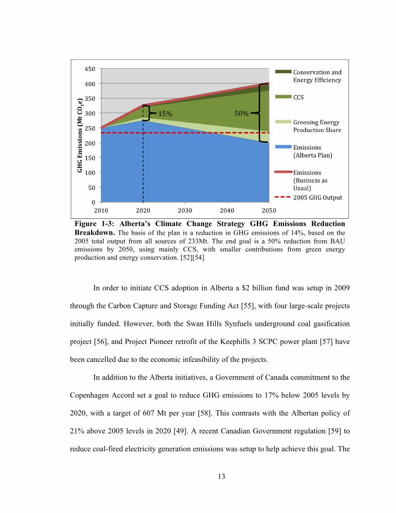
(BAU) case by 2020 and 50% below by 2050, as demonstrated in Figure 1-3. This is a

province wide initiative that affects all industries, such as oil and gas and electricity

producers. The reduction target is equivalent to 200Mt CO2e per year, resulting in a

reduction of 14% below 2005 levels in 2050 [52] (marked on Figure 1-3 as a red dashed

line). The specified paths to achieve this goal (and their respective shares of the 200Mt

reduction), demonstrated in Figure 1-3 as components of the green shaded area, are

through the use of CCS (139Mt), an increase of green energy technologies (37Mt), and an

increase in conservation and energy efficiency (24Mt). The electric sector is expected to

take a large portion of this reduction, since in 2011 it was responsible for around 35% of

the registered [51], and 20% of the total GHG emissions in Alberta [53].

13

Figure 1-3: Alberta’s Climate Change Strategy GHG Emissions Reduction Breakdown. The basis of the plan is a reduction in GHG emissions of 14%, based on the 2005 total output from all sources of 233Mt. The end goal is a 50% reduction from BAU emissions by 2050, using mainly CCS, with smaller contributions from green energy production and energy conservation. [52][54]

In order to initiate CCS adoption in Alberta a $2 billion fund was setup in 2009

through the Carbon Capture and Storage Funding Act [55], with four large-scale projects

initially funded. However, both the Swan Hills Synfuels underground coal gasification

project [56], and Project Pioneer retrofit of the Keephills 3 SCPC power plant [57] have

been cancelled due to the economic infeasibility of the projects.

In addition to the Alberta initiatives, a Government of Canada commitment to the

Copenhagen Accord set a goal to reduce GHG emissions to 17% below 2005 levels by

2020, with a target of 607 Mt per year [58]. This contrasts with the Albertan policy of

21% above 2005 levels in 2020 [49]. A recent Canadian Government regulation [59] to

reduce coal-fired electricity generation emissions was setup to help achieve this goal. The

14

regulation, starting in 2015, sets intensity limits of coal power plants to below 420 t/GWh

or levels in the range of high efficiency NGCC plants [59]. This policy effectively

mandates the retirement of coal power plants, or the adoption of CCS technology to

comply with the regulations.

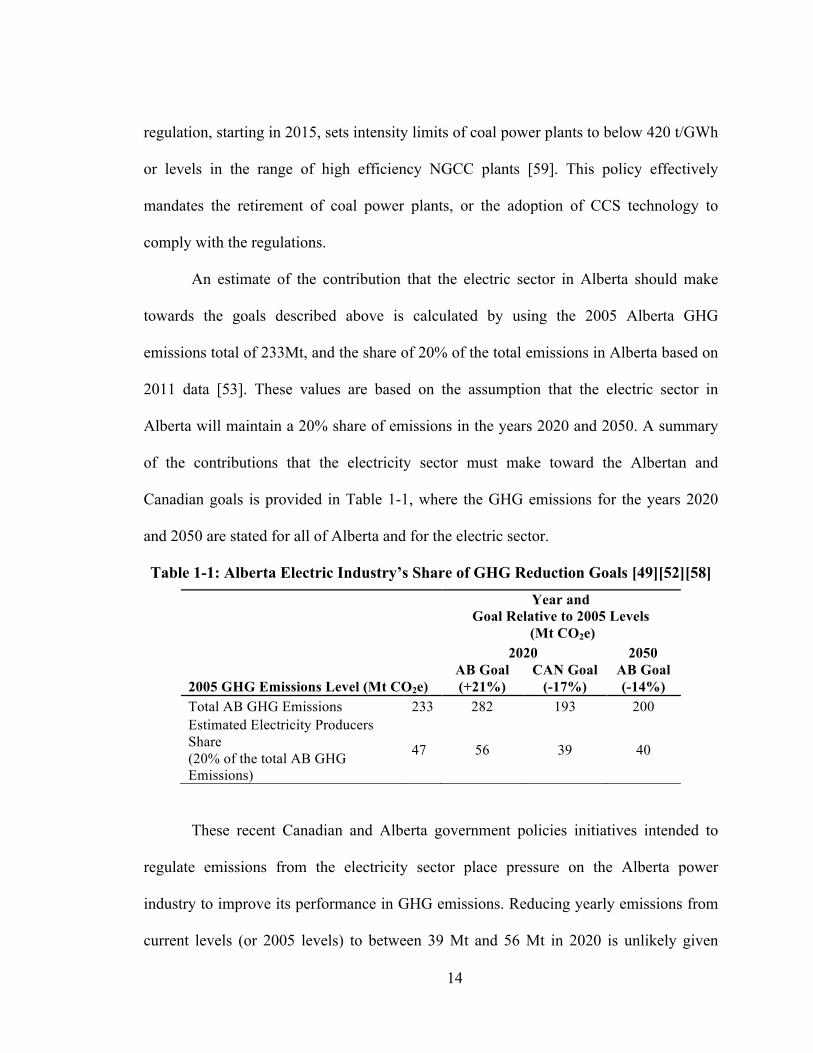
An estimate of the contribution that the electric sector in Alberta should make

towards the goals described above is calculated by using the 2005 Alberta GHG

emissions total of 233Mt, and the share of 20% of the total emissions in Alberta based on

2011 data [53]. These values are based on the assumption that the electric sector in

Alberta will maintain a 20% share of emissions in the years 2020 and 2050. A summary

of the contributions that the electricity sector must make toward the Albertan and

Canadian goals is provided in Table 1-1, where the GHG emissions for the years 2020

and 2050 are stated for all of Alberta and for the electric sector.

Table 1-1: Alberta Electric Industry’s Share of GHG Reduction Goals [49][52][58]

2005 GHG Emissions Level (Mt CO2e)

Year and Goal Relative to 2005 Levels

(Mt CO2e) 2020 2050

AB Goal (+21%)

CAN Goal (-17%)

AB Goal (-14%)

Total AB GHG Emissions 233 282 193 200 Estimated Electricity Producers Share (20% of the total AB GHG Emissions)

47 56 39 40

These recent Canadian and Alberta government policies initiatives intended to

regulate emissions from the electricity sector place pressure on the Alberta power

industry to improve its performance in GHG emissions. Reducing yearly emissions from

current levels (or 2005 levels) to between 39 Mt and 56 Mt in 2020 is unlikely given

15

Alberta’s slow transition to less GHG intensive technologies. Reducing to 40 Mt in 2050

will require substantial technological changes in Alberta’s electric sector. Switching to

NG power generation alone is not likely to achieve these targets, making emissions-

reducing technologies, such as CCS necessary to achieve emissions targets set by both

governments.

There are several technological paths that can be taken to reduce GHG emissions.

While renewable energy technologies in Alberta are currently a minority contributor (i.e.,

on the order of 10% currently [45]), they are increasing and many efforts are underway to

make them more competitive. However, because Alberta is rich in fossil fuels, CCS

incorporated with thermal power generation is a leading option to reduce GHG

emissions. However, to date, CCS has yet to come to fruition in the electric sector. To

counter this, NG is playing the role of a transitional fuel, by providing a 50% reduction in

stack emissions below coal fired power without carbon capture and storage. It seems

Alberta has options to choose from in reducing GHG emissions, but a clear choice has yet

to be made.

Based on the available resources and current electricity generation technology in

use in Alberta, there are two prominent fossil fuel pathways for future development in

power generation: coal and NG. The first pathway is the use of clean coal technologies,

such as supercritical or ultra supercritical pulverized coal technologies. Alberta has about

70% of the coal reserves in Canada, which amounts to about 33 Gt of remaining reserves

and 620 Gt of ultimate potential [60]. This abundance of fuel makes the use of coal

technologies attractive. The inclusion of CCS with clean coal technologies would

facilitate electricity production development to meet GHG targets such as the

16

Government of Alberta’s Climate Change Strategy [52] (i.e., 14% below 2005 levels in

2050 [52]) and the Government of Canada’s incoming regulation on coal power (i.e., a

limit of 420t/GWh or levels in the range of high efficiency NGCC plants [59] by 2015).

While this technology is currently cost prohibitive, it is ready for full scale deployment

[61], there are several pilot projects [62][63], and one full scale project set to start

operation in Saskatchewan by 2014 [64]. Additionally, there are several techno-economic

studies assessing coal technologies with CCS to further knowledge on this topic (e.g.,

[37][38][65]). Factors such as the potential for future high NG prices and carbon taxes

also provide incentive to pursue this path.

The second pathway uses NGCC. In this pathway, coal is phased out due to

regulatory pressure, while the switch to NGCC allows producers to conform. While this

pathway achieves substantial GHG emissions reduction (i.e., roughly half of current

levels) it will not be enough to reach current GHG goals. To counter this, there is a

possibility that producers may incorporate CCS technology at some point in the future.

However, the costs and performance of NGCC with CCS are highly uncertain, and future

additional carbon mitigation policy is currently undefined.

There is a high degree of uncertainty in evaluating NGCC with CCS as compared

to coal with CCS for four reasons. First, there is a lack of experimental data about how

the advanced CCS technology will perform and be integrated into a NGCC plant, making

modeling the technology difficult. Currently, based on data from the Global CCS Institute

project database, only one of 32 power generation projects with CCS are NGCC based

[62]. Second, the economics of NGCC with CCS are highly uncertain. The share of the

fuel cost in NGCC is greater than pulverised coal [66] and the cost of NG is prone to

17

wide fluctuations when looking at long time frames [67]. There is consensus on the

stability of the price of NG in the short term [9][45], however it is prone to large long-

range price fluctuations [67]. There is a risk that this pathway could be much more costly

in the long run if NG prices rise. Additional to fuel prices, there is uncertainty

surrounding the utilization (the percentage of time the plant is operational over one year)

of NGCC plants, with an estimated increase in costs of 50% if the plants are used for

intermediate or peak loads rather than base loads [26]. For example, over the past two

decades NGCC plants in the U.S. have had rates of 30% to 50% [68]. Third, there is the

potential for increased life cycle (LC) GHG emissions of this pathway due to the nature

of extraction of unconventional NG [69][70]. Finally, there are technological

uncertainties surrounding the capture of CO2 in NGCC plants due to the dilute carbon

dioxide in the flue gas (compared to PC plants) [71]. Consequently, the uncertainty

analysis focus in the following case study is within the NGCC (not the coal) pathway.

There are several risks associated with this the NGCC pathway that should be

considered by decision makers. There is likely to be a delay in implementation of CCS on

NG until there is a breakthrough in the technology, such that the capital costs are more

reasonable and progress is made in addressing the problems associated with the more

dilute concentration of CO2 in the flue gas. Essentially, there is a distinct possibility that

CCS may never be adopted. There is also a possibility that fuel prices will rise to the

point where NGCC with CCS may be less economic when compared to other

alternatives. Additionally, risks associated with increased upstream emissions from

unconventional NG extraction should also be addressed.

18

The case study is structured to inform industry and policy makers with a focus on

the improvement in performance and cost that would be needed for a CCS technology to

break into the market. A potential question faced by decision and policy makers here is;

“Is switching to NG fired generation technologies an effective long term GHG reduction

plan?” The case study explores the impacts of short term GHG emissions reduction and

assesses the risks associated with waiting for NG CCS technologies to become more

feasible before implementing them. Additionally, questions surrounding the long-term

costs and upstream impacts of switching fuel may be of concern. For this analysis, an

NGCC amine capture technology, with performance and cost parameters based on

available data, is used to represent the increase in fuel required and associated increase in

stack and upstream GHG emissions characteristic of CCS use. However, the use of amine

technology does not imply that it is the preferable technology, nor the most likely

technology to succeed in future full-scale deployment.

In order to answer the above question, the case study applies the framework to the

Alberta electricity generation in order to assess various alternatives to satisfy electricity

demand over one hundred years, while incorporating the uncertainty associated with an

advanced NGCC CCS technology. Four scenarios are modeled, 1) a baseline scenario

where no CCS technology is deployed, 2) a scenario where coal is phased out and

replaced with NGCC, and two additional scenarios representing potential competing

alternative GHG reducing pathways 3) NGCC with a highly uncertain advanced CCS

technology deployed at a future date and 4) supercritical pulverized coal (SCPC) with a

more mature CCS technology deployed immediately. The uncertainty assessment

component of the framework is then applied to assess the influence of the uncertainty of

19

the NGCC advanced capture technology on the outcomes and options available for

Alberta. Renewable energy technologies are not in the scope of this thesis and therefore

are not modelled in more detail along with an associated detailed analysis of their impact

in future scenarios. Renewable energy sources are considered an important component in

future electricity production in Alberta and are represented within the analysis as a

percentage of the total energy produced in the system. Additionally, since the role of

renewables is consistent among the case study scenarios, their impact will have no effect

on the relative results between scenarios. The purpose of the framework is to evaluate an

advanced carbon capture technology but could eventually be modified to evaluate other

energy technologies, including renewables.

5 Thesis Overview and Contributions

Evaluating CCS technologies at an early stage of development will help to

prioritize research and development, improve process designs, as well as help to avoid

unintended consequences. The thesis approaches this problem by combining a developed

numerical model (created to model an electric power system) and a set of uncertainty

assessment tools using MATLAB [44]. This thesis presents a means for a system-wide

techno-economic assessment of advanced CCS technologies, with a more robust analysis

of the inherent uncertainties than previous studies in the field (e.g., [26][28][32-34][36-

40][72]), with the goal of providing useful information to decision makers. This thesis

contributes to the international field of LCA by demonstrating how the integration of

uncertainty assessment with LCC and LCA can help inform decisions on emerging

energy technologies. Specifically, the developed framework explores the environmental

and cost trade-offs involved in implementing an advanced CCS technology. The

20

framework can be adapted more broadly to a range of energy system investment

decisions involving technologies with high degrees of uncertainty and where other less

uncertain competing technology options exist. Additionally, the framework will be used

to evaluate an emerging CCS technology in the context of a case study. In doing so, the

thesis provides insight into the choices available to Alberta, when considering GHG

mitigation technologies.

Chapter Two chapter provides a review of the literature relevant to the

development of the framework by reviewing existing studies in the area of Life Cycle

Assessment, Life Cycle Costing, and Energy System Modeling, and uncertainty

assessment methods in existing energy studies, with a focus on CCS technology

applications. A review of existing frameworks and models used to perform energy system

analysis is conducted to assess methods and structures used in other technology

assessments.

Chapter Three describes the method behind the development of the framework in

two main sections. The first section describes the creation of a generic numerical

MATLAB [44] model that represents an electric power system that satisfies demand

based on the inputs and choices supplied by a user. The model satisfies the demand for

electricity using a given long range forecast, and a specified mix of generation

technologies. Deterministic results in both cost and environmental performance are

generated on a yearly and total basis over the timeline. The second section describes the

conception of the uncertainty assessment aspect of the framework. This component

assesses the source of the uncertainty in the results from the numerical model using

various sensitivity analyses, and quantifies the uncertainty to create probabilistic results.

21

The methods surrounding the creation of the case study are then presented. Data related

to Alberta’s electricity system along with a selection of generation technologies is

selected and discussed based on the chosen scenarios. Parameters related to the NGCC

CCS technology and other uncertain aspects are explored, with ranges of values

presented.

Chapter Four demonstrates the use of the framework in the Alberta case study

discussed above. Four scenarios chosen for the analysis, representing alternative options

to satisfy electric energy demand, are presented and discussed. The results from the

analysis are analyzed in the context of Alberta’s electricity generation future, with an

assessment of each scenario based on individual performance (against GHG emissions

targets) and relative performance (comparing probabilistic results through ranking).

Chapter Five then offers concluding remarks regarding the implications of the

analysis towards broader Life Cycle Assessment applications, with discussion

surrounding the implications of the case study and the options available to Alberta for

reducing GHG emissions. Some implications to broader policy issues are also discussed.

Finally, Chapter Five concludes with some future potential research questions and some

recommendations regarding the applicability of this framework to evaluate other

emerging technologies.

 

22

References

[1] International Energy Agency, "CO2 Emissions From Fuel Combustion: Highlights," 2012.

[2] R. E. H. Sims, H.-H. Rogner, and K. Gregory, "Carbon emission and mitigation cost comparisons between fossil fuel, nuclear and renewable energy resources for electricity generation," Energy Policy, vol. 31, no. 13, pp. 1315-1326, Oct 2003.

[3] J. P. Painuly, "Barriers to renewable energy penetration; a framework for analysis," Renewable Energy, vol. 24, no. 1, pp. 73-89, Sep 2001.

[4] IEA, Energy Technology Perspectives 2012: OECD Publishing, 2012. [5] N. E. Hultman, J. G. Koomey, and D. M. Kammen, "What History Can Teach Us

About the Future Costs of U.S. Nuclear Power," Environmental Science & Technology, vol. 41, no. 7, pp. 2087-2094, May 16 2007.

[6] R. Sathre, M. Chester, J. Cain, and E. Masanet, "A framework for environmental assessment of CO2 capture and storage systems," Energy, vol. 37, no. 1, pp. 540-548, Feb 01 2012.

[7] National Energy Board, "Canada's Oil Sands Opportunities and Challenges to 2015: An Update," Government of Canada 0-662-43353-X, 2006.

[8] G. H. Doluweera, S. M. Jordaan, M. C. Moore, D. W. Keith, and J. A. Bergerson, "Evaluating the role of cogeneration for carbon management in Alberta," Energy Policy, vol. 39, no. 12, pp. 7963-7974, Dec 01 2011.

[9] Alberta Energy, "Generation Additions Since 1998," Alberta Energy, 2012. [10] U. S. E. I. Administration, "Net Generation for Electric Utility Annual," U.S.

Energy Information Administration, 2013. [11] National Energy Board, "Canada's Energy Future," National Energy Board,

Ottawa, ON, 2011. [12] Statistics Canada, "Report on Energy Supply and Demand in Canada,"

Government of Canada, Ottawa, ON, Annual Report, May 30 2013. [13] Alberta Utilities Commission, "Annual Electricity Data Collection ": Alberta

Utilities Commission, 2013. [14] U.S. Energy Information Administration, "Emissions of Greenhouse Gases in the

United States," Washington, DC, April 2011. [15] National Energy Board, "Short-term Canadian Natural Gas Deliverability,"

Government of Canada, Jun 2013. [16] W. Moomaw, F. Yamba, M. Kamimoto, L. Maurice, J. Nyboer, K. Urama, and T.

Weir, "Introduction. In IPCC Special Report on Renewable Energy Sources and Climate Change Mitigation," United Kingdon and New York, NY, USA, 2011.

[17] H. J. Herzog, "Scaling up carbon dioxide capture and storage: From megatons to gigatons," Energy Economics, vol. 33, no. 4, pp. 597-604, Jul 01 2011.

[18] J. A. Bergerson and L. Lave, "The long-term life cycle private and external costs of high coal usage in the US," Energy Policy, vol. 35, no. 12, pp. 6225-6234, 2007.

[19] G. P. Hammond, S. S. O. Akwe, and S. Williams, "Techno-economic appraisal of fossil-fuelled power generation systems with carbon dioxide capture and storage," Energy, vol. 36, no. 2, pp. 975-984, Mar 2011.

23

[20] J. C. Stephens and S. Jiusto, "Assessing innovation in emerging energy technologies: Socio-technical dynamics of carbon capture and storage (CCS) and enhanced geothermal systems (EGS) in the USA," Energy Policy, vol. 38, no. 4, pp. 2020-2031, May 01 2010.

[21] J. D. Sharp, M. K. Jaccard, and D. W. Keith, "Anticipating public attitudes toward underground CO2 storage," International Journal of Greenhouse Gas Control, vol. 3, no. 5, pp. 641-651, Sep 2009.

[22] Global CCS Institute. The Global Status of CCS: 2013, 2013 [Online]. Available: http://www.globalccsinstitute.com/publications/global-status-ccs-2013/online/117741 accessed on Nov 04 2013

[23] E. S. Rubin, S. Yeh, M. Antes, M. Berkenpas, and J. Davison, "Use of experience curves to estimate the future cost of power plants with CO2 capture," International Journal of Greenhouse Gas Control, vol. 1, no. 2, pp. 188-197, 2007.

[24] Carbon Capture & Sequestration Technologies MIT Energy Initiative. (2013). Power Plant Carbon Dioxide Capture and Storage Projects. Massachussetts Institute of Technology, 2013 [Online]. Available: http://sequestration.mit.edu/tools/projects/index_capture.html accessed on 5 September 2013

[25] E. S. Rubin, H. Mantripragada, A. Marks, P. Versteeg, and J. Kitchin, "The outlook for improved carbon capture technology," Progress in Energy and Combustion Science, vol. 38, no. 5, pp. 630-671, 2012.

[26] E. S. Rubin and H. Zhai, "The Cost of Carbon Capture and Storage for Natural Gas Combined Cycle Power Plants," Environmental Science & Technology, vol. 46, no. 6, pp. 3076-3084, Apr 20 2012.

[27] E. S. Rubin and H. Zhai, "The Cost of CCS for Natural Gas-Fired Power Plants," in 10th Annual Conference on Carbon Capture and Storage, Pittsburgh, Pennsylvania, 2011, Jun 03.

[28] E. S. Rubin, C. Chen, and A. B. Rao, "Cost and performance of fossil fuel power plants with CO2 capture and storage," Energy Policy, vol. 35, no. 9, pp. 4444-4454, 2007.

[29] K. C. Hoffman and D. O. Wood, "Energy System Modeling and Forecasting," Annual Review of Energy, vol. 1, no. 1, pp. 423-453, 1976.

[30] N. A. Odeh and T. T. Cockerill, "Life cycle analysis of UK coal fired power plants," Energy Conversion and Management, no., pp. 2008.

[31] I. F. Roth and L. L. Ambs, "Incorporating externalities into a full cost approach to electric power generation life-cycle costing," Energy, vol. 29, no. 12–15, pp. 2125-2144, Dec 01 2004.

[32] M. Pehnt and J. Henkel, "Life cycle assessment of carbon dioxide capture and storage from lignite power plants," International Journal of Greenhouse Gas Control, vol. 3, no. 1, pp. 49-66, Feb 2009.

[33] N. A. Odeh and T. T. Cockerill, "Life cycle GHG assessment of fossil fuel power plants with carbon capture and storage," Energy Policy, vol. 36, no. 1, pp. 367-380, 2008.

24

[34] P. Jaramillo, W. M. Griffin, and H. S. Matthews, "Comparative Life-Cycle Air Emissions of Coal, Domestic Natural Gas, LNG, and SNG for Electricity Generation," Environmental Science & Technology, vol. 41, no. 17, pp. 6290-6296, Sep 2007.

[35] H. Baumann and A. M. Tillman, The Hitch Hiker's Guide to LCA. Lund, Sweden: Studentlitterature, 2004.

[36] H. Lund and B. V. Mathiesen, "The role of Carbon Capture and Storage in a future sustainable energy system," Energy, vol. 44, no. 1, pp. 469-476, Aug 01 2012.

[37] C.-C. Cormos, "Integrated assessment of IGCC power generation technology with carbon capture and storage (CCS)," Energy, vol. 42, no. 1, pp. 434-445, Jul 01 2012.

[38] H. Zhai and E. S. Rubin, "A Techno-Economic Assessment of Polymer Membrane Systems for Post-combustion Carbon Capture at Coal-fired Power Plants," Environmental Science & Technology, no., pp. 130213162018003, Mar 13 2013.

[39] U.S. Department of Energy’s National Energy Technology Laboratory, "Life Cycle Analysis: Natural Gas Combined Cycle (NGCC) Power Plant," U.S. Department of Energy’s National Energy Technology Laboratory, Sep 302010.

[40] P. Versteeg and E. S. Rubin, "Technical and economic assessment of ammonia-based post-combustion CO2 capture," Energy Procedia, vol. 4 IS -, no., pp. 1957-1964, 2011.

[41] G. F. Nemet, E. Baker, and K. E. Jenni, "Modeling the future costs of carbon capture using experts elicited probabilities under policy scenarios," 8th World Energy System Conference, WESC 2010, vol. 56, no. 0, pp. 218-228, Jul 2013.

[42] K. Johnsen, K. Helle, and T. Myhrvold, "Scale-up of CO2 capture processes: The role of Technology Qualification," Greenhouse Gas Control Technologies 9 Proceedings of the 9th International Conference on Greenhouse Gas Control Technologies (GHGT-9), 16–20 November 2008, Washington DC, USA, vol. 1, no. 1, pp. 163-170, Mar 01 2009.

[43] V. Rai, D. G. Victor, and M. C. Thurber, "Carbon capture and storage at scale: Lessons from the growth of analogous energy technologies," Energy Policy, vol. 38, no. 8, pp. 4089-4098, Aug 2010.

[44] "MATLAB," 2013b ed. Natick, Massachusetts: The Mathworks Inc, 2013. [45] Alberta Electric System Operator, "AESO Long-term Transmission Plan," Jul 01

2012. [46] Alberta Utilities Commission. (2013). Annual Electricity Data Collection, 2013

[Online]. Available: http://www.auc.ab.ca/market-oversight/Annual-Electricity-Data-Collection/Pages/default.aspx accessed on Saturday, April 13 2013

[47] National Energy Board, "Coal-Fired Power Generation: A Perspective," Government of Canada, Calgary, AB July 2008.

[48] Canadian Association of Petroleum Producers, Upstream Dialogue: The Facts on Oil Sands: Canadian Association of Petroleum Producers, 2013.

25

[49] J. P. Pfeifenberger and K. Spees, "Evaluation of Market Fundamentals and Challenges to Long-Term System Adequacy in Alberta’s Electricity Market," The Brattle Group, 2011.

[50] Government of Alberta, "Climate Change and Emissions Management Act: Specified Gas Emitters Regulation," Government of Alberta, ed. Edmonton, Alberta: Alberta Queen's Printer, 2007.

[51] Alberta Environment and Sustainable Development. (2013). 2012 Greenhouse Gas Emission Reduction Program Results. Alberta Environment and Sustainable Development,, 2013 [Online]. Available: http://environment.alberta.ca/04220.html accessed on 21 September 2013

[52] Alberta Environment, "Alberta’s 2008 Climate Change Strategy," Government of Alberta, 978-0-7785-6789-9, Feb 2008.

[53] Alberta Environment and Sustainable Development. (2013). Regulating Greenhouse Gas Emissions. Government of Alberta, 2013 [Online]. Available: http://environment.alberta.ca/0915.html accessed on September 30, 2013

[54] Alberta Environment, "Alberta Environment Report on 2006 Greenhouse Gas Emissions," Edmonton, AB, 2007.

[55] Government of Alberta, "Carbon Capture and Storage Funding Act," Government of Alberta, ed. Edmonton, Alberta: Alberta Queens Printer, 2009.

[56] R. Blackwell. (2013). Alberta cancels funding for carbon capture project. The Globe and Mail, 2013 [Online]. Available: http://www.theglobeandmail.com/report-on-business/industry-news/energy-and-resources/alberta-cancels-funding-for-carbon-capture-project/article9024237/ accessed on 21 September 2013

[57] C. Tait. (2013). Alberta's carbon capture efforts set back. The Globe and Mail, 2012 [Online]. Available: http://www.theglobeandmail.com/report-on-business/industry-news/energy-and-resources/albertas-carbon-capture-efforts-set-back/article4103684/ accessed on 21 September, 2013

[58] Environment Canada, "Canada's Emission Trends 2012," Government of Canada,, Ottawa, Ontario, 2012.

[59] Government of Canada, "Reduction of Carbon Dioxide Emissions from Coal-fired Generation of Electricity Regulations (SOR/2012-167), Canadian Environmental Protection Act, 1999," Government of Canada, ed. Ottawa, Ontario: Minister of Justice, 2012.

[60] Alberta Energy. Coal Statistics - Coal Reserves and Resources as of Dec 31, 2012. Government of Alberta, 2012 [Online]. Available: http://www.energy.alberta.ca/coal/643.asp accessed on September 2, 2013

[61] G. T. Rochelle, "Amine Scrubbing for CO2 Capture," Science, vol. 325, no. 5948, pp. 1652-1654, Sep 24 2009.

[62] Global CCS Institute, "Status of CCS Project Database," Global CCS Institute, 2013.

[63] Global CCS Institute, "The Global Status of CCS," Global CCS Institute. [64] C. C. a. S. T. P. a. MIT. Boundary Dam Fact Sheet: Carbon Dioxide Capture and

Storage Project. MIT, 2013 [Online]. Available:

26

http://sequestration.mit.edu/tools/projects/boundary_dam.html accessed on 5 October 2013

[65] G. Xu, L. Duan, M. Zhao, Y. Yang, J. Li, L. Li, and H. Chen, "Performance Analysis of Existing 600MW Coal-Fired Power Plant with Ammonia-Based CO2 Capture," in 2010 International Conference on Electrical and Control Engineering (ICECE): IEEE, 2010, pp. 3973-3976.

[66] U.S. Department of Energy’s National Energy Technology Laboratory, "Cost and Performance Baseline for Fossil Energy Plants, Revision 2.," Pittsburgh, PA DOE/NETL-2010/1397, November, 2010.

[67] US Energy Information Administration. (2013). Henry Hub Gulf Coast Natural Gas Spot Price (Dollars/Mil. BTUs). US Energy Information Administration, 2013 [Online]. Available: http://www.eia.gov/dnav/ng/hist/rngwhhda.htm accessed on 17 September 2013

[68] Energy Information Administration, "Annual Energy Review 2009," Washington, DC, August, 2010.

[69] M. Jiang, W. Michael Griffin, C. Hendrickson, P. Jaramillo, J. VanBriesen, and A. Venkatesh, "Life cycle greenhouse gas emissions of Marcellus shale gas," Environmental Research Letters, vol. 6, no. 3, pp. 034014, Aug 05 2011.

[70] R. W. Howarth, R. Santoro, and A. Ingraffea, "Methane and the greenhouse-gas footprint of natural gas from shale formations," Climatic Change, vol. 106, no. 4, pp. 679-690, May 12 2011.

[71] C. A. Grande, R. P. P. L. Ribeiro, and A. r. E. Rodrigues, "CO2 Capture from NGCC Power Stations using Electric Swing Adsorption (ESA)," Energy & Fuels, vol. 23, no. 5, pp. 2797-2803, Jun 21 2009.

[72] G. F. Nemet, E. Baker, and K. E. Jenni, "Modeling the future costs of carbon capture using experts' elicited probabilities under policy scenarios," Energy, vol. 56, no. 0, pp. 218-228, Jul 2013.

CHAPTER TWO: Literature Review

1 Introduction

The premise behind this thesis is to provide an integrated technology assessment

framework for researchers to evaluate advanced carbon capture and storage (CCS)

technologies with a system wide life cycle (LC) perspective and an explicit treatment of

the unique uncertainties present in emerging technologies. The goal of the framework is

to present the trade-offs associated with their use in a manner that accounts for

uncertainty (i.e., through probability distributions) and generate information regarding the

use of the advanced CCS technology so that decision makers can make informed policy

and investment decisions.

The conceptual use of the framework, depicted graphically in Figure 1-1, provides

results in terms of life cycle cost and life cycle GHG emissions performance. The

framework uses a baseline set of data for electricity generation technology, CCS

technology, and electricity system information (i.e., demand and generation mix). The

framework includes two main components: an integrated life cycle model and an

uncertainty assessment model. The integrated life cycle model uses Energy System

Modeling (ESM), Life Cycle Assessment (LCA) and Life Cycle Costing (LCC) methods

to model a system of various electricity producing technologies. An uncertainty

assessment model is developed to address the different sources and natures of uncertainty

inherent in the evaluation of the advanced capture technology using various methods.

Results from the framework are presented for use in a multi-criteria assessment, which

allows evaluation of the trade-offs between cost and environmental performance.

28

Figure 2-1: Concept of Framework Use in Advanced CCS Technology Evaluation. The framework requires baseline data to generate results that are used in an assessment using multiple criteria. The framework contains two components, an Integrated LC Model and an Uncertainty Assessment Model to generate the results.

This chapter provides a review of the literature relevant to the development of the

framework. LC methods and uncertainty assessment methods in existing energy studies,

with a focus on CCS technology applications are reviewed as well as existing

frameworks and models that are used to perform energy system analysis.

2 Literature Review of ESM, LCA, and LCC of CCS Technologies

The methods that were chosen to be included in the Integrated LC Model are

ESM, LCA, and LCC. LCA is a systematic analytical tool that can be used to evaluate the

environmental and economic impacts of a product or process, from the extraction of raw

materials to the use and/or disposal of waste products, or “cradle to grave” [1]. LCA

typically involves the following four stages. The first stage sets the goal and scope of the

study. Here a model of the material or energy flow of the process under investigation is

developed, with physical boundaries determined and documented. Second, a life cycle

inventory analysis is performed which creates the data set (i.e., inputs and outputs) used

29

in the study. Subsequently, a mass and energy balance is conducted throughout the

model and the resulting emissions (or other environmental flows of concern) are

calculated. The third stage of LCA is called the Impact Assessment, where impacts of the

environmental flows are determined (e.g., global warming potential, or resource

depletion). A final stage, called the Interpretation Stage, where this thesis makes a

contribution, is used to take the results from the Impact Assessment and draw conclusions

from them. This stage may involve going back to the first three stages and make

adjustments, or it may involve using different methods of manipulating the results (such

as sensitivity or uncertainty analysis) to look at the conclusions in a different light (i.e.,

an analysis to assess the robustness of the results and conclusions).

LCC is a systematic method for assessing the total cost of a facility ownership

(e.g., a power plant) [2]. It takes into account all costs of building, owning and operating,

and disposal of the facility system. LCC is useful when comparing power plant

alternatives that have similar energy output specifications but differ with respect to

capital and operating costs. This method can be used to select the alternative that

maximizes the net savings (i.e., the operational savings resulting from the use of the

alternative less difference in capital investment costs). For example, in meeting a given

level of electricity demand, two power plant alternatives with the same output, one coal

and one natural gas, can be compared. LCC considers the balance between the higher

capital costs of coal power and the generally higher operating costs of natural gas power.

When combined with LCA, the trade-off between environmental performance (GHG

emissions) and the cost to produce electricity can be presented in a comprehensive and

consistent manner.

30

Research in LCA can be generally divided into four themes; assessment of

environmental impacts (e.g., [3][4]), research into the methodology of LCA (e.g., [5][6]),

the integration of LCA into tools to help inform decision-making (e.g., [7][8]), and a

combination of the latter to model the effects of public policy (e.g., [9]). Investigation of

CCS technologies using LCA and LCC is extensive (e.g., [10-16]). The majority of these

studies use LCA and LCC to conduct plant level analysis for comparison to other

technologies. For example, Pehnt and Henkel [14] uses LCA to study lignite coal power

plants with all three different types of CCS. They use the study to quantify the magnitude

of the increased energy demand of the plants and the decreased emissions resulting from

the inclusion of CCS. They also assessed other environmental impacts, such as

acidification. They did not, however, use LCC to investigate the economic implications.

In another study, Jamarillo et al. [10] performed a LCA that compared NG generation

technologies fuelled from imported and domestic NG supplies to coal generation

technologies, with and without CCS. The purpose of the study is to compare coal power

production to NG power production different sources of NG. The study assesses the

potential impacts of increased use of Liquefied Natural Gas (LNG) and Synthetic Natural

Gas (SNG), both of which they calculate can have higher upstream GHG emissions than

conventional NG production. They determine that the use of LNG and SNG still resulted

in less overall LC emissions when compared to coal. Odeh and Cockerill [13] assessed

Pulverized Coal (PC), NGCC, and Integrated Gasification Combined Cycle (IGCC)

power plants with CCS using a LCA. Their LCA system boundaries include the

production of material (e.g., capture system chemicals) and disposal of material (e.g.,

solid waste and waste water) used in the CCS processes, and the production and

31

transportation of fuel in addition to the GHG emitted from the power plant. This study

challenged the general consensus that a 90% CO2 capture rate is typical, by

demonstrating that the actual percentage of CO2 captured is less at around 75-84%,

through accounting for other stages where increased energy consumption occurs. They

note that for NGCC plants the amount of methane leakage from NG extraction and

transport has a significant effect on LC GHG emissions (+10.9% over a reference system

with a 2% increase in NG loss), which is exacerbated in the NGCC CCS system due to

the required increase in fuel consumption (+33.2% over a reference system with a 2%

increase in NG loss). The studies described here demonstrate the utility of LCA and LCC

in the evaluation of the environmental impacts and costs associated with CCS. Despite

the utility of LCA and LCC, there are some potential drawbacks that are considered next.

The use of LCA and LCC for evaluating CCS technologies requires specific

considerations in order to produce comprehensive results useful for decision makers.

Sathre et al. [15] comment that the analysis of CCS technologies is complex, and

therefore propose a framework for environmental LCA of CCS technologies. They

discuss seven key issues that they reasoned should be addressed when using LCA to

evaluate CCS. The first is the energy penalty imposed by CCS technologies. They

recommend that LCA practitioners use appropriate estimates for the energy penalty and

use a system wide approach (a system of plants rather than an individual plant) that

accounts for the impacts of CCS deployed in large scale. Examples of impacts accounted

for are the increased LC GHG emissions due to increased fuel requirements for plants

with CCS and the reduction in the whole system efficiency. The second issue was the

relationship between functional units and demand for electricity. The functional unit is

32

defined as the quantitative measure of the function of the studied system, which provides

a reference to which the inputs and outputs can be related, and a basis for comparison of

different (competing) systems. Here Sathre et al. state that the functional unit normally

used in LCA studies, per kWh of deliverable electricity, does not fully indicate the impact

on the overall system if only the plant level is studied. They reason that, for example, the

overall implications of a less efficient system that includes CCS plants should be

reflected in the choice of functional unit. They suggest using multiple functional units

where additional functions of the system are present (e.g., enhanced oil recovery or heat

supplied by combined heat power systems), or a system wide approach that accounts for

the required additional electricity supply to make up for the reduction caused by CCS use

in other plants. The third issue was the consideration of non-climate impacts in the LCA

study. They reason that the inclusion of CCS should not reduce GHG at the expense of

some other environmental impact, ergo a wider picture should be considered in LCA. A

fourth issue is the suggested inclusion of uncertainty management. They suggest that a

wide consideration of uncertainty be reflected in LCA, such as including treatment for

parameter, model, and scenario uncertainties. A fourth concern, scale-up issues, is

discussed. They suggest that the magnitude of CO2 captured required to achieve the goal

of CCS (i.e., deep reductions in GHG emissions), requires a scale-up of perhaps a

thousand times above current levels. Three issues in scaling up are discussed;

technological, analytical, and operational scale. They recommend that LCA practitioners

consider non-linear changes in CCS LCA. Beneficial economies of scale or detrimental

material resource constraints were provided as example situations. In the fifth issue,

policy-making needs, they discuss the function that LCA can play in a policy-making

33

role. They reason that, in some cases, structuring CCS LCAs around prospective GHG

reduction policies would be more beneficial than just performing retrospective analyses

that quantify the GHG footprints of different technologies. They suggest that use of life

cycle costing will help to further this goal. The final issue suggested in this study was

market effects (i.e., the broader market reactions to CCS use). Policy impacts from

market effects, and vice versa, are suggested to contribute to uncertainty in the results and

therefore limit the LCA recommendations. They suggest the consideration of a range of

behaviours (e.g., from local actors versus remote actors) that may affect the

environmental performance of the larger system. An example of this might be an increase

in water consumption resulting from increased NG production using hydraulic fracturing

to meet the increase in NG demand resulting from switching to NG from coal. They

conclude that LCA should aim to provide holistic information on the implications of CCS

deployed at scale, system wide, and with a reflection of the complexity involved in its

use.

LCA and LCC combined offer a systematic means to evaluate the trade-offs

involved in CCS technologies. However, there are certain criteria that should be

addressed in order to properly inform decision makers. The concepts highlighted by

Sathre et al. [15] are further developed and applied to this thesis including the

construction of a model that:

1) represents a system wide electricity demand-supply system over a

long time period (on the order of several decades);

2) represents upstream GHG impacts;

3) includes both cost and GHG impacts;

34

4) incorporates the ability to include uncertainty in scale-up effects;

5) presents results relevant to policy making needs;

6) and allows for the inclusion of uncertainty assessment.

There is a paucity of studies, which use both LCA and LCC in a long-term

evaluation of advanced CCS technologies. By adopting the considerations of experts in

the area of ESM, LCA and LCC and applying the model with long-term boundaries, the

current study fills this gap in the literature.

3 Literature Review of Uncertainty Assessment Methods

A wide body of literature exists on the topic of uncertainty assessment in energy

analysis. Some researchers have recognized the importance of considering uncertainty in

LCA studies involving emerging energy technologies. In Heijungs and Kleijn’s [17] work

on numerical approaches to the interpretation stage of LCA they spoke to the loss of data

and information that can occur during the data reduction and analysis processes within

LCA studies. Others, such as Hung et al. [18], looked at the broader LCA process (i.e.,

four stages) and examined which part would lead to the primary uncertainty. They stated

that most studies focus on uncertainty in individual stages and individual parameters of

LCA. They reasoned that understating the contributions that each stage of LCA makes

toward the total uncertainty would improve the study and make it more credible.

Others have attempted to predict the result of not fully exploring the effects of

uncertainty. For example, a recent study by Rubin et al. [19], notes that published

estimates of future electricity costs for power plants with advanced CCS offer optimistic

projections of cost reductions. They opine that technologies tend to look better the further

they are from commercial reality. Johnsen et al. [20] attempts to identify sources

35

uncertainty in advanced CCS technologies by speaking to the issues of scaling up to

industrial capacity. They discuss the technological challenges of scaling up carbon

capture technologies from pilot or lab scale projects. They suggest that the critical aspects

of scale-up relate to the impact of ratios (e.g., between surface to volume, height to

diameter, and gas to liquid) on dispersion and heat transfer [20]. They add that the nature

of the scaling problem may be physical, chemical, or both. For example, calculating the

size of the equipment required in the larger system is critical to maintaining optimal

reaction performance [20]. They conclude that, for advanced CCS technologies, the order

of magnitude of the scale-up would result in very large equipment to accommodate the

flue gas volumes, presenting operational and design challenges.

Some recent studies investigate the nature of uncertainty and have attempted to

characterize sources of uncertainty with the goal of achieving a better understanding of

the nature and treatment of this issue. Lloyd and Ries [21] survey 24 LCA studies and

present findings regarding the methods of uncertainty assessment in LCA. To provide

organization to the survey, regarding the sources of uncertainty, they propose a structure

centered on the three main components of LCA as defined by the U.S. Environmental

Protection Agency [22], parameters used, scenarios represented, and models used. Within

those components they propose the sources of uncertainty based on work by Morgan and

Henrion [23]. Examples of the sources are: random error, systematic error, variability,

and approximation. The result of this approach suggests various sources of uncertainty

for each LCA component. For parameters used in the LCA, sources of uncertainty are

identified as variability, measurement imprecision, and data quality issues in LCA

studies. In the scenarios used in LCA studies they suggest the uncertainty in the

36

normative choices used to create scenarios as a main source of uncertainty. In addition,

they mention the inherent variability of scenario data due to geographic locations (e.g.,

different costs of capital in different countries). For the third component, models used in

LCA, they suggest uncertainties arise due to the imprecise nature of modeling the real

world, or inconstancies between models used in LCA studies. This study provides a

framework to characterize uncertainty in LCA that is adapted and applied within this

thesis.

Based on the available literature it is evident that the nature of uncertainty is of

concern when evaluating emerging energy technologies, and in particular emerging

advanced CCS technologies. This uncertainty, if not treated explicitly in a proper manner,

can lead to false outcomes, overly optimistic results, and results that do not reflect the

associated probability of the outcomes. In order to create more robust and relevant results

various studies present sensitivity analysis methods to identify factors or parameters that

most affect the results through parameter variability [6][10][13][17][24]. Jamarillo et al.

[10] use error bars to represent uncertainty in the results of a LCA that compares NG

generation technologies fuelled from imported NG supplies to coal generation

technologies, with and without CCS. However, they do not analyze the variability with

any additional methods. Others use various sensitivity analyses to explore the sources of

uncertainty in a more comprehensive manner. For example, Cormos [24] uses a

sensitivity analysis with a tornado plot to rank the parameters with the most influence on

CO2 emissions avoidance cost results in an assessment of IGCC technology with CCS. In

another example, Odeh and Cockerill [13] use a similar sensitivity analysis to determine

that LC GHG emissions of CCS technologies are more sensitive to variation in capture

37

efficiency than the variation in length of transport pipeline (i.e., fugitive emissions of

CO2 during transportation to a storage site). To provide structure to sensitivity analyses,

Heijungs and Klein [17] propose numerical steps that can be used in the interpretation

stage of LCA studies to check completeness and sensitivity of data. First, a contribution

analysis is proposed, where the result is broken up into the contributing processes, and

displayed in a way that makes the largest contributors identifiable (e.g., system

component contributions to total GHG emissions). Second, a perturbation analysis is

recommended where small fluctuations in parameters are performed while the changes in

results are recorded. Two values are calculated based on the observations, a Sensitivity

Ratio (SR) and a Sensitivity Coefficient (SC). These values can then be used to create a

ranked list of parameters that are the most influential to the results, signifying the

parameters that require particular attention and further analysis. Claverul et al. [6] use a

Combined Sensitivity Analysis (CSA) to explore the effects of simultaneous variation in

two parameters on results. This analysis is useful in that it can demonstrate how the

ranking changes between two scenarios for different combinations of values of the

chosen two parameters. However, the CSA used by Claverul et al. does not include

uncertainty propagation (i.e., the uncertainty in the outcome resulting from the

uncertainty in the input parameters), and therefore could not include uncertainty

quantification, thereby providing no probability of ranking change. This thesis improves

on this method by using uncertainty propagation in combination with the CSA procedure.

Several studies demonstrate the use of sensitivity analyses to point to sources of

uncertainty, provide a structured analysis of parameter variation effects, and establish

important parameters that affect results to inform further analyses [6][10][13][17][24].

38

However, others suggest that care be taken when performing sensitivity analysis. Saltelli

and Annoni [25] discuss the importance of careful sensitivity analysis, and highlight the

shortcomings of sensitivity analysis methods that vary one parameter at a time. They

suggest that this type of sensitivity analysis (the most common) can lead to incorrect

results, especially in systems with nonlinear relationships. Additionally, all of the

aforementioned studies use deterministic methods in the sensitivity analysis, which does

not fully account for or quantify the uncertainty.

Other studies have used methods of quantifying uncertainty in results by

propagating the uncertainty in parameters through model calculations. Parameters are

represented in a stochastic manner that allows for random sampling using different

methods. A large number of random samples, N, from chosen parameters (i.e., those of

most interest, or the largest source of uncertainty) are past through a model or equation N

times, for N results. Monte Carlo methods are common choices for sampling methods.

These are computational algorithms that use repeated random sampling of input

probabilities to derive a probability distribution of the result [23]. There are several

examples of Monte Carlo Simulation (MCS) being used to quantify the uncertainty

within LCA studies (e.g., [7][18][26-28]). Another example, Sills et al. [29] use a MCS

approach to assess the effect of uncertainty in determining outcomes within a LCA for

biofuels. They use empirically specified distribution functions for the inputs based on

values obtained from previously published LCA studies of algal biofuel production. They

then quantified the uncertainty in the results, which allows for a more informed

assessment of the outcomes. Rather than simple ranges in the values of the results, a

probability distribution is created, which allows for comparison of alternate outcomes

39

that includes probabilities associated with the results. In another example, Rubin et al.

[28] use the MCS capabilities within the IECM [30] software to provide a probabilistic

analysis of key parameters to quantify uncertainty in costs of NGCC power plants with

CCS. This provides an assessment of the likely costs in a statistically significant manner.

A drawback of MCS is that the quality of the results it produces is based on the quality of

the input data [21]. Another drawback to MCS is that it requires many samples to fully

represent input distributions, and can leave out the tails (extreme ends) if under

represented resulting in outcomes that exclude the areas of least probability (i.e., extreme

events) or those that might be of the most interest to researchers [31].

There are methods to improve on MCS, such as with Latin Hypercube Sampling

(LHS), which is another method of uncertainty propagation [25][32]. LHS is similar to

MCS in that it samples from probability distributions, however, it does it in a way that

samples equally across the distribution by dividing the sampling space into equally

probable strata [33][34]. This is opposed to sampling from the entire distribution as in

MCS, where the tail ends of the distribution tend to be sampled from the least. Strata

from each input variable are sampled in random order. Saltelli and Paola [25] suggest the

benefit of using LHS is to maximize the exploration of the input distributions, without

compromising efficiency in the procedure. Brohus et al. [31] study the uncertainty of

energy consumption in domestic buildings by using MCS with LHS to ensure a proper

representation of the true variability in the parameters used. A MCS routine by itself can

provide a similar representation, but may require double the iterations [31].

Two caveats are associated with MCS. The first is that the analyzed parameters

should not have a mathematical relationship to each other, since the sampling in MCS is

40

done independently without consideration of a relationship [21]. The second is that input

distributions should be represented using the highest quality data available in order to

obtain the most robust result [21]. Some researchers have explored the methods of

representing the input distributions used in MCS. For example, Lloyd and Ries [21] state

that the use of simple probability distributions (without exploring the actual nature of the

system) used in uncertainty propagation can lead to false outcomes. To address this issue,

Nemet et al. [35] uses MCS using Expert Elicitation to represent the uncertainty in input

parameters. In their study on modeling the future costs of CCS, they use expert elicitation

to create input distributions in the cost and performance parameters of their model. On

the other hand, others like Sill et al. [29] recognize the importance of proper input

representation, but face a lack of data. They state their assumption that there is no

correlation among the parameters used within the MCS and that they do not know the

accuracy of the probability distributions used. Faced with a lack of real data to input into

the simulation, users of MCSs must find alternate sources of data that still allow

relatively robust results of the uncertainty analysis, or test the effects of the assumptions

made on the results using a sensitivity analysis. The analysis of the literature provides

little evidence of this occurring in LCAs, and consequently there is very little literature

on the methods and outcomes of doing this type of analysis. This thesis explores this in

more detail than has been done before for CCS technologies.

Scenario and model (as opposed to parameter) uncertainty in LCAs and other

techno-economic studies have been treated (i.e., explicitly assessed) in various ways.

Some use scenario analysis to explore the effects of uncertainty in options and choices

available in selecting technology to reduce GHG emissions. Pehnt, et al. [14] use scenario

41

analysis within a LCA of CCS for lignite power plant technologies to assess the effect of

technology choice (between pulverized coal with and with out CCS, IGCC with and with

out CCS, and oxyfuel with CCS) in GHG mitigation. Viebahn et al. [36] use three

scenarios for solar power adoption rates to deal with the uncertainty associated with

future technology deployment rate. However, in both cases they do not propagate the

uncertainty in parameters used in the evaluation and therefore do not quantify the effects

of the uncertainty. Others use MCS to propagate uncertainty through multiple scenarios,

and then compare the resulting distributions of the scenario outcomes. For example,

Clavreul et al. [6] use this method to compare uncertainty in a LCA of two waste

management systems.

Others propose systematic methods to explore data and assess the impacts of

uncertainty in LCA studies. In their work on creating an integrated approach to

uncertainty consideration in LCA, Basson and Petrie [7] consider both technical

uncertainties (in estimation of the potential consequences of activities) and valuation

uncertainties (in variables used in the evaluation). Their goal is to promote effective

decision-making in LCA by providing a foundation for the consideration of the

implications of diversity in values. They propose three key elements of the approach;

placing appropriate bounds on parameters, ensuring that results regarding the alternatives

are adequately statistically distinguishable by performing a distinguishability analysis,

propagating uncertainties and performing a sensitivity analysis. In the same theme,

Heijungs and Klein [17] recommend an uncertainty analysis (along with the sensitivity

methods mentioned earlier) to quantify the uncertainty in the study. In this case, as

demonstrated by [7][18][26-28], MCS or LHS is useful. Additionally, they recommend a

42

comparative analysis (i.e., a structured means to compare results, such as tables and

charts) followed by a discernibility analysis (which is comparable to Basso and Petrie’s

[7] distinguishability analysis) to compare the results of the uncertainty analysis. Claverul

et al. [6] builds on the work by Heijungs and Klein by building a framework, and then

demonstrating it using a waste management LCA example. Their study is useful in that it

provides a structured approach to uncertainty analysis, using various methods to explore

the sources and quantify the uncertainty. Another example on proposing a framework is

by Sathre et al. [15]. Here, in a challenge to researchers to provide structure around

uncertainty in CCS analysis, they propose key issues, that should be considered to

adequately inform the decision making process (e.g., energy penalty, functional units,

scale-up challenges, uncertainty management). Thus, they present requirements for a

framework for environmental assessment for CCS systems and suggested "LCA should

aim to describe the system-wide environmental implications of CCS deployment at scale,

rather than a narrow analysis of technological performance of individual power plants"

[15].

The literature reviewed in this chapter presents several methods for considering

uncertainty in technology assessment. There are many ways to explore, treat and quantify

the uncertainty. Sensitivity methods (e.g., contribution analysis, perturbation analysis,

combined sensitivity analysis, scenario analysis) can be used to provide a general

overview of the important parameters and assumptions used in a study. Uncertainty

propagation analysis methods (e.g., MCS and LHS) can be used to quantify the

uncertainty, and with the help of comparison analysis methods (e.g., discernibility

analysis) can be used to present the results. These analyses can be organized with the

43

LCA and LCC methods discussed above into a structured framework to systematically

extract and present meaningful information relevant to researchers and decision makers.

The contribution from this thesis is that it provides more detailed assessment of the

effects of uncertainty inherent in CCS technologies than current studies and pushes the

methods for quantifying and incorporating uncertainty into decision-making contexts.

The thesis also proposes stochastic sensitivity methods to test assumptions made in

representing the uncertainty (through probability distributions) of parameters. This issue

is not well explored in the field of LCA, and few methods exist. The methods used and

the framework proposed can be applied more broadly by providing a means to more

accurately assess, quantify, and incorporate uncertainty in into LCA studies of other

emerging energy technologies.

4 Literature Review of Existing Energy System Models and Frameworks

Existing energy system modeling and decision-making frameworks are reviewed

here in order to survey potential tools and methods that could be used in the framework.

Two existing studies have completed surveys similar to this project. Finnveden and

Moberg [37] survey and categorize environmental systems analysis tools. Some examples

of tools are Life Cycle Assessment, Life Cycle Costing, and Cost Benefit Analysis, all of

which have bearing on the current framework. However, because their analysis looked at

more general methods as opposed to specific models or computer programs, their

research did not provide a usable LC model that this thesis endeavours to do. Another

was a study by Connolly et al. [38]. They review 37 existing energy system computer

analyses that can be used to analyze the integration of renewable energy technologies.

They can be categorized into seven basic types, as proposed by Connolly et al. [38].

44

First, simulation tools simulate the operation of an energy system and provide

results in sets of energy demands over a series of years. For example, AEOLIUS [39] is a

power plant dispatch simulation that “analyses the impact of higher penetration rates of

fluctuating energy carriers such as wind and PV, on conventional power-plant systems”

[38]. BALMOREL [40] simulates electricity and heat sectors by geographical

subdivision with flexible time units and can analyze electricity storage, transmission,

cost, SO2 and NOx. Simulation tools provide big-picture views and most often have

secondary functions such as those in the later categories.

The second category is scenario tools. Scenario tools differ from simulation tools

by combining series of years into long-term scenarios. BALMOREL [40], as discussed

above, can be used as a scenario tool. Another example is EMINENT [41], a tool

designed to be a catalyst for introducing new energy technologies into the market.

EMINENT [41] includes a database and an assessment tool, which allows performance

evaluations of early stage technologies in a pre-defined energy supply chain for a defined

number of years. RETScreen [42] is a software tool designed to quickly evaluate the

energy production, life cycle costs, and life cycle emissions reductions for various types

of renewable energy technologies (RET) and cogeneration projects [38]. It focuses on the

implementation of clean energy technologies within a specified grid and on the financial

aspects of the project. It uses five steps for project analysis; energy model design, cost

analysis, GHG emissions analysis, financial summary, and sensitivity and risk analysis

[43]. In the sensitivity and risk analysis step, a Monte Carlo Simulation (MCS) is used for

financial risk assessment. It is available free of charge and available to download from

the RETScreen Internet website. RETScreen focuses on RET and has little or no ability

45

for CCS technology evaluation. The uncertainty assessment component is limited in

flexibility and is restricted to the economics in the model. Though scenario tools have a

large time range, they typically simulate scenarios anywhere from 20-50 years.

The third computer tool category for integration analysis is Equilibrium. These

tools attempt to relate the behavior of parts of an economy, such as supply, demand, or

prices, with several or many markets. For example, E4cast [44] is an Australian partial-

equilibrium tool that provides detailed analyses of their national energy system by

considering production, trade, and consumption and projects energy consumption by fuel,

industry and region. Another example, ENPEP-BALANCE [45], matches energy demand

with available resources. In a study by McFarland et al. [46] they present a methodology

for modeling low-carbon emitting technologies within the MIT Emissions Prediction and

Policy Analysis (EPPA) model [47], a general equilibrium model. They use a system

wide approach (representing the U.S. electricity production sector) to modeling new

energy technologies by using a bottom-up technology cost method (i.e., representing

individual energy technologies with a high level of cost detail) to improve on top-down

economic models (i.e., aggregated high level systems). They present the study with an

example that assesses the market penetration of NG technologies (with and without CCS)

while competing with other technologies in a carbon-constrained economy. They analyze

the effect of changes in fuel and input prices, and carbon policy on the production share

that each technology has over 100 years. While this study presents a relevant method to

model an energy system with various technologies to satisfy electricity demand over

several decades, it does not explicitly treat the uncertainty in costs and performance of

the technologies investigated. Furthermore, the study does not include LCA in the

46

method, thereby excluding the environmental impacts of upstream GHG emissions.

These models have an underlying assumption that equilibrium can be reached within the

system.

The fourth category consists of top-down macroeconomic tools. These tools use

general macroeconomic data to model the growth in both energy demand and prices.

Top-down tools are most often also equilibrium tools. ENPEP-BALANCE [45], in

addition to being an Equilibrium tool, is also an example of a top-down assessment tool.

Long-range Energy Alternatives Planning, or LEAP [48], is an integrated modeling tool

that produces outputs which resemble storylines of how an energy system could evolve

over time and is capable of analyzing the impact of demand and pricing on energy

systems, among other things. The Canadian Energy Systems Simulator (CanESS) [49] is

a tool developed by whatIf Technologies Inc. that represents Canada’s entire energy

supply and demand system. The modeling scheme uses human activities and the

associated flow of energy and resources to provide feedback on emissions. It is a very

flexible model, allowing users to customize it to suit their needs. Steenhof and McInnis

[50] use CanESS to compare the results of different low carbon transportation scenarios

for Canada. In the study, they use data to calibrate the model to achieve the desired

analysis. A drawback to this model is that it does not provide much more than emissions

and resource depletion as environmental loads, and requires additional techno-economic

data for detailed carbon capture technology analysis, which is difficult and time

consuming to incorporate due to the proprietary nature of the software. In addition it does

not allow for integrated uncertainty analysis.

47

Bottom-up tools identify and assess energy technologies in order to identify

investment options. One model already discussed, AEOLIUS [39] is capable of bottom-

up analysis, as is BALMOREL [40] and EMINENT [41]. The BCHP Screening Tool [51]

is a much smaller-scale tool than previous examples in that it assesses the savings

potential of combined cooling, heating, and power systems for single buildings. It does

bottom-up analyses by performing parametric analyses between a baseline building and

alternative building scenarios. The Integrated Environmental Control Module (IECM)

[30], developed by Carnegie Mellon University, is an electricity generation technology

analysis tool developed for calculating the performance, emissions, and cost of a single

fossil-fuelled power plant. It has capabilities to model several coal technologies and

Natural Gas Combined Cycle (NGCC) with various different CCS technology options.

Users are able to customize the plant design by changing the input of various

performance and cost parameters. Costs and performance parameters have been recently

updated to 2011 values. It has integrated uncertainty analysis limited to Monte Carlo

Simulation, and it is not a system wide analysis tool. However, data for the performance

of the power plants are accessible and can be used to generate plant level models for

integration into a system wide model. Several CCS technology studies have been

conducted using IECM (e.g., [52][53l][54]). For example, in a study by Nemet et al. [35]

they use IECM [30] data to produce models that are reduced in form (modelling that

summarizes several plant processes and variables) when compared to IECM [30]. These

models are then used to estimate the costs of CCS under different policy scenarios. The

idea behind using reduced models, as stated by Nemet et al., is to allow flexibility and

full control over model behaviour when uncertainty analysis is performed in the study, to

48

allow for a broader range of capital cost assumptions and parameter uncertainty, and to

allow for the inclusion of a single CCS energy penalty factor rather than several factors.

The sixth category used by Connolly et al. [38] is labeled Operation Optimization.

As the name implies, these tools optimize the operation of a given energy system. The

BCHP Screening Tool discussed above optimizes the operation of buildings by providing

up to 25 alternate scenarios to compare to baseline in order to provide the user with the

best possible economic and climate scenarios. COMPOSE [55] is a tool that evaluates

how capable an energy project is at supporting intermittency while offering a realistic

assessment of cost/benefit distributions under uncertainty. Operation optimization tools

usually use simulation methods. EnergyPLAN [56] is deterministic computer model

developed by the Sustainable Energy Planning Research group at Aalborg University in

cooperation with PlanEnergi and EMD A/S. It was developed to assist the design of

national or regional energy planning strategies by simulating the entire system in a

deterministic manner [38][57]. It also optimizes the operation of an energy system, based

on inputs (e.g., demands, technologies, cost specifications) and outputs (e.g., energy

balances, fuel consumption, totals costs) rather than just the economic costs alone.

EnergyPLAN [56] has a maximum timeframe of one year, with time steps of one hour. It

does not provide detailed environmental impacts of the simulations other than CO2

emissions, but does provide the resulting costs associated with technology choices. It has

limited capacity for uncertainty assessment, and does not include a detailed CCS

technology evaluation component or the ability to build it in to the model. MARKAL

[58] and TIMES [59] are powerful operation optimization energy assessment tools

developed by International Energy Agency’s ‘‘Energy Technology Systems Analysis

49

Programme.” They are used for global to community level analysis of energy-

environment inputs and resulting costs and externalities of technology use [38][60]. They

allow for all thermal, storage, conversion, and transportation technologies to be included

in a given system. The model generators have been used to create several tailored models

for various purposes, such as perspectives on achieving a low carbon society [61] and

CCS integration and evaluation [62]. They have limited uncertainty assessment

capabilities including stochastic modeling and sensitivity analysis [63]. The issue with

MARKAL and TIMES is that, through artificially constraining the model, they select the

least cost path, even if two pathways are pennies apart.

Finally, Investment Optimization tools are similar to operation optimization, but

they seek to optimize investment in an energy system. COMPOSE [55] and the BCHP

Screening Tool [51] both have investment optimization capabilities. E4cast [44], because

its primary use is for analyzing the national energy sector, naturally includes investment

optimization as well. These tools generally are also scenario tools.

While the models, frameworks, and studies listed above all deal with emerging

energy technology to some degree, none include all five factors deemed integral to

informing policy on advanced CCS technology: LCA, LCC, uncertainty assessment,

system wide analysis, and long term projections. This thesis addresses these five points

within an integrated life cycle framework.

What is lacking in the realm of CCS technology evaluation is a framework that

rigorously assesses the inherent uncertainties and considers the system wide effects of

deployment on a large scale. The literature survey conducted in this section of the thesis

provides several examples of tools, approaches, and methods for assessing energy

50

technology impacts and for assessing and treating uncertainty in a structured manner.

Together, they provide a set of insights that can be used to construct the framework.

There are many methods to model an electricity energy system. In considering a

method to model an electricity energy system some key characteristics are considered

essential. First the model should be flexible and adaptable in that it allows a variety of

customizable technology options with modifiable parameters. Second, the model must be

able to conduct or interface with a robust uncertainty analysis with several types of

analyses. And lastly, the model should be able to represent an electricity production

system over a long time period (i.e., several decades).

51

References

[1] H. Baumann and A. M. Tillman, The Hitch Hiker's Guide to LCA. Lund, Sweden: Studentlitterature, 2004.

[2] D. M. Kammen and S. Pacca, "Assessing the Costs of Electricity," Annual Review of Environment and Resources, no. 29, pp. 301-44, 2004.

[3] J. A. Bergerson, O. Kofoworola, A. D. Charpentier, S. Sleep, and H. L. MacLean, "Life Cycle Greenhouse Gas Emissions of Current Oil Sands Technologies: Surface Mining and In Situ Applications," Environmental Science & Technology, vol. 46, no. 14, pp. 7865-7874, Feb 26 2013.

[4] A. D. Charpentier, O. Kofoworola, J. A. Bergerson, and H. L. MacLean, "Life Cycle Greenhouse Gas Emissions of Current Oil Sands Technologies: GHOST Model Development and Illustrative Application," Environmental Science & Technology, vol. 45, no. 21, pp. 9393-9404, Feb 26 2013.

[5] K. G. Canter, D. J. Kennedy, D. C. Montgomery, J. B. Keats, and W. M. Carlyle, "Screening stochastic Life Cycle assessment inventory models," The International Journal of Life Cycle Assessment, vol. 7, no. 1, pp. 18-26, Feb 2002.

[6] J. Clavreul, D. Guyonnet, and T. H. Christensen, "Quantifying uncertainty in LCA-modelling of waste management systems," Waste Management, vol. 32, no. 12, pp. 2482-2495, Dec 2012.

[7] L. Basson and J. G. Petrie, "An integrated approach for the consideration of uncertainty in decision making supported by Life Cycle Assessment," Environmental Modelling & Software, vol. 22, no. 2, pp. 167-176, Mar 01 2007.

[8] I. Linkov, "Coupling Multi-Criteria Decision Analysis, Life-Cycle Assessment, and Risk Assessment for Emerging Threats - Environmental Science & Technology (ACS Publications)," Environmental Science & Technology, no., pp. 2011.

[9] S. Ross, D. Evans, and M. Webber, "Using LCA to examine greenhouse gas abatement policy," The International Journal of Life Cycle Assessment, vol. 8, no. 1, pp. 19-26, 2003.

[10] P. Jaramillo, W. M. Griffin, and H. S. Matthews, "Comparative Life-Cycle Air Emissions of Coal, Domestic Natural Gas, LNG, and SNG for Electricity Generation," Environmental Science & Technology, vol. 41, no. 17, pp. 6290-6296, Sep 2007.

[11] U.S. Department of Energy’s National Energy Technology Laboratory, "Life Cycle Analysis: Natural Gas Combined Cycle (NGCC) Power Plant," U.S. Department of Energy’s National Energy Technology Laboratory, Sep 302010.

[12] National Energy Technology Laboratory, "Role of Alternative Energy Sources: Natural Gas Technology Assessment," DOE/NETL-2012/1539,2012.

[13] N. A. Odeh and T. T. Cockerill, "Life cycle GHG assessment of fossil fuel power plants with carbon capture and storage," Energy Policy, vol. 36, no. 1, pp. 367-380, 2008.

[14] M. Pehnt and J. Henkel, "Life cycle assessment of carbon dioxide capture and storage from lignite power plants," International Journal of Greenhouse Gas Control, vol. 3, no. 1, pp. 49-66, Feb 2009.

52

[15] R. Sathre, M. Chester, J. Cain, and E. Masanet, "A framework for environmental assessment of CO2 capture and storage systems," Energy, vol. 37, no. 1, pp. 540-548, Feb 01 2012.

[16] A. Schreiber, P. Zapp, and W. Kuckshinrichs, "Environmental assessment of German electricity generation from coal-fired power plants with amine-based carbon capture," The International Journal of Life Cycle Assessment, vol. 14, no. 6, pp. 547-559-559, 2009.

[17] R. Heijungs and R. Kleijn, "Numerical approaches towards life cycle interpretation five examples," The International Journal of Life Cycle Assessment, vol. 6, no. 3, pp. 141-148, Jun 01 2001.

[18] M.-L. Hung and H.-w. Ma, "Quantifying system uncertainty of life cycle assessment based on Monte Carlo simulation," The International Journal of Life Cycle Assessment, vol. 14, no. 1, pp. 19-27, Oct 14 2008.

[19] E. S. Rubin, H. Mantripragada, A. Marks, P. Versteeg, and J. Kitchin, "The outlook for improved carbon capture technology," Progress in Energy and Combustion Science, vol. 38, no. 5, pp. 630-671, 2012.

[20] K. Johnsen, K. Helle, and T. Myhrvold, "Scale-up of CO2 capture processes: The role of Technology Qualification," Greenhouse Gas Control Technologies 9 Proceedings of the 9th International Conference on Greenhouse Gas Control Technologies (GHGT-9), 16–20 November 2008, Washington DC, USA, vol. 1, no. 1, pp. 163-170, Mar 01 2009.

[21] S. M. Lloyd and R. Ries, "Characterizing, Propagating, and Analyzing Uncertainty in Life-Cycle Assessment: A Survey of Quantitative Approaches," Journal of Industrial Ecology, vol. 11, no. 1, pp. 161-179, Oct 2008.

[22] U.S. EPA, "Exposure Factors Handbook," Washington, DC, USA Report EPA/600/8-89/043,1989.

[23] M. G. Morgan, M. Henrion, and M. Small, Uncertainty: A Guide to Dealing with Uncertainty in Quantitative Risk and Policy Analysis. Cambridge, UK: Cambridge University Press, 2003.

[24] C.-C. Cormos, "Integrated assessment of IGCC power generation technology with carbon capture and storage (CCS)," Energy, vol. 42, no. 1, pp. 434-445, Jul 01 2012.

[25] A. Saltelli and P. Annoni, "How to avoid a perfunctory sensitivity analysis," Environmental Modelling & Software, vol. 25, no. 12, pp. 1508-1517, Dec 01 2010.

[26] D. Yue, P. Khatav, F. You, and S. B. Darling, "Deciphering the uncertainties in life cycle energy and environmental analysis of organic photovoltaics," Energy Environ. Sci., vol. 5, no. 11, pp. 9163-9172, 2012.

[27] P. Versteeg and E. S. Rubin, "Technical and economic assessment of ammonia-based post-combustion CO2 capture," Energy Procedia, vol. 4 IS -, no., pp. 1957-1964, 2011.

[28] E. S. Rubin and H. Zhai, "The Cost of Carbon Capture and Storage for Natural Gas Combined Cycle Power Plants," Environmental Science & Technology, vol. 46, no. 6, pp. 3076-3084, Apr 20 2012.

53

[29] D. L. Sills, V. Paramita, M. J. Franke, M. C. Johnson, T. M. Akabas, C. H. Greene, and J. W. Tester, "Quantitative Uncertainty Analysis of Life Cycle Assessment for Algal Biofuel Production," Environmental Science & Technology, vol. 47, no. 2, pp. 687-694, Feb 15 2013.

[30] Carnegie Mellon University, "The Integrated Environmental Control Model (IECM)," 8.0.2 ed: Carnegie Mellon University, 2013.

[31] H. Brohus, P. Heiselberg, and A. Simonsen, "Uncertainty of energy consumption assessment of domestic buildings," in Proceedings of the 11th International Building Performance Simulation Association (IBPSA) Conference, 2009, pp. 27-30.

[32] U. M. Diwekar and J. R. Kalagnanam, "Efficient sampling technique for optimization under uncertainty," AIChE Journal, vol. 43, no. 2, pp. 440-447, 1997.

[33] M. D. Mckay, R. J. Beckman, and W. J. Conover, "A Comparison of Three Methods for Selecting Values of Input Variables in the Analysis of Output From a Computer Code," Technometrics, vol. 42, no. 1, pp. 55-61, Mar 01 2000.

[34] M. A. J. Huijbregts, "Application of uncertainty and variability in LCA," The International Journal of Life Cycle Assessment, vol. 3, no. 5, pp. 273-280, Sep 1998.

[35] G. F. Nemet, E. Baker, and K. E. Jenni, "Modeling the future costs of carbon capture using experts elicited probabilities under policy scenarios," 8th World Energy System Conference, WESC 2010, vol. 56, no. 0, pp. 218-228, Jul 2013.

[36] P. Viebahn, Y. Lechon, and F. Trieb, "The potential role of concentrated solar power (CSP) in Africa and Europe—A dynamic assessment of technology development, cost development and life cycle inventories until 2050," Energy Policy, vol. 39, no. 8, pp. 4420-4430, Aug 01 2011.

[37] G. Finnveden and Å. Moberg, "Environmental systems analysis tools – an overview," Journal of Cleaner Production, vol. 13, no. 12, pp. 1165-1173, Oct 2005.

[38] D. Connolly, H. Lund, B. V. Mathiesen, and M. Leahy, "A review of computer tools for analysing the integration of renewable energy into various energy systems," Applied Energy, vol. 87, no. 4, pp. 1059-1082, May 2010.

[39] Universität Karlsruhe. AEOLIUS. Institute for Industrial Production. [Online]. Available: http://www.iip.kit.edu/65.php accessed on 10 November 2013

[40] H. Ravn. Balmorel [Online]. Available: http://www.balmorel.com/ accessed on [41] EMINENT2. Welcome to EMINENT [Online]. Available:

http://www.eminentproject.com accessed on 10 November 2013 [42] CanmetENERGY Core Team, "RETScreen Software Suite," 4 ed: Natural

Resources Canada, Government of Canada, 2013. [43] RETScreen® International Clean Energy Decision Support Centre, Clean Energy

Project Analysis: RETScreen® Engineering & Cases Textbook, vol. Third Edition: Natural Resources Canada, 2005.

[44] ABARE. ABARE models [Online]. Available: http://www.abare.gov.au/publications_html/models/models/models.html accessed on 10 November 2013

54

[45] Argonne National Laboratory. ENPEP-BALANCE. Energy and Power Evaluation Program (ENPEP-BALANCE) [Online]. Available: http://www.dis.anl.gov/projects/Enpepwin.html accessed on 10 November 2013

[46] J. R. McFarland, J. M. Reilly, and H. J. Herzog, "Representing energy technologies in top-down economic models using bottom-up information," Energy Economics, vol. 26, no. 4, pp. 685-707, Jul 2004.

[47] M. H. M. Babiker, J. M. Reilly, M. Mayer, I. Sue Wing, R. C. Hyman, and R. S. Eckaus, "The MIT Emissions Prediction and Policy Analysis (EPPA) model : revisions, sensitivities, and comparisons of results," MIT Joint Program on the Science and Policy of Global Change, 2001.

[48] Stockholm Environment Institute. LEAP. Community for energy, environment and development [Online]. Available: http://www.energycommunity.org/ accessed on 10 November 2013

[49] WhatIf Technologies, "Canadian Energy Systems Simulator (CanESS)," 2011. [50] P. A. Steenhof and B. C. McInnis, "A comparison of alternative technologies to

de-carbonize Canada's passenger transportation sector," Technological Forecasting and Social Change, vol. 75, no. 8, pp. 1260-1278, Oct 2008.

[51] Oak Ridge National Laboratory. BCHP Screening Tool. Whole-Building and Community Integration Program [Online]. Available: http://www.coolingheatingpower.org/about/bchp-screening-tool.php accessed on 10 November 2013

[52] C. Chen and E. S. Rubin, "CO2 control technology effects on IGCC plant performance and cost," Energy Policy, vol. 37, no. 3, pp. 915-924, 2009.

[53] A. B. Rao and E. S. Rubin, "A Technical, Economic, and Environmental Assessment of Amine-Based CO 2Capture Technology for Power Plant Greenhouse Gas Control," Environmental Science & Technology, vol. 36, no. 20, pp. 4467-4475, Oct 01 2002.

[54] H. Zhai and E. S. Rubin, "Comparative Performance and Cost Assessments of Coal and Natural-Gas-Fired Power Plants under a CO2 Emission Performance Standard Regulation," Energy & Fuels, vol. 27, no. 8, pp. 4290-4301, Feb 05 2013.

[55] Aalborg University. COMPOSE EnergyInteractive.NET [Online]. Available: http://energyinteractive.net accessed on 10 November 2013

[56] Sustainable Energy Planning Research Group, "EnergyPLAN," 10.0 ed: Aalborg University, 2012.

[57] H. Lund, "EnergyPLAN - Advanced Energy Systems Analysis Computer Model," Document Version 10, August 2012.

[58] Energy Technology Systems Analysis Program, "MARKAL," International Energy Agency, 2001.

[59] Energy Technology Systems Analysis Program, "TIMES," International Energy Agency, 2007.

[60] R. Loulou, M. Labriet, and A. Kanudia, "ETSAP-TIAM (TIMES Integrated Assessment Model)," 2007.

55

[61] U. Remme and M. Blesl, "A global perspective to achieve a low-carbon society (LCS): scenario analysis with the ETSAP-TIAM model," Climate Policy, vol. 8, no. sup1, pp. S60-S75, Feb 04 2013.

[62] S. Teir, E. Tsupari, A. Arasto, T. Koljonen, J. Kärki, A. Lehtilä, L. Kujanpää, S. Aatos, and M. Nieminen, "Prospects for application of CCS in Finland," Greenhouse Gas Control Technologies 9 Proceedings of the 9th International Conference on Greenhouse Gas Control Technologies (GHGT-9), 16–20 November 2008, Washington DC, USA, vol. 4, no. 0, pp. 6174-6181, 2011.

[63] R. Loulou, U. Remne, A. Kanudia, A. Lehtila, and G. Goldstein, "Documentation for the TIMES Model: PART I," Energy Technology Systems Analysis Programme, 2005.

56

CHAPTER THREE: Methods

1 Introduction

1.1 Chapter Overview

This chapter describes the development and application of a framework to assess

advanced carbon capture technologies. The goal of this thesis is to provide a tool for

researchers to evaluate advanced CCS technologies and present the trade-offs so that

industry and government decision-makers can make informed policy and investment

decisions regarding the use of the technology. A secondary goal of the thesis is to apply

the framework using a case study.

Based on the review of existing frameworks, it was decided that the development

of the framework using the MATLAB [1] programing language was the best course of

action. The technology assessment framework presented in this chapter has two main

components; an Integrated Life Cycle Electricity Production Model (henceforth referred

to as the Integrated LC Model) to evaluate electricity production in a system of power

plants in terms of cost and environmental performance, and an Uncertainty Assessment

Model that uses a variety of methods to characterize and analyze the uncertainty inherent

in evaluation of these technologies. A graphical representation of the required framework

components is provided in Figure 3-1. The Integrated LC Model and the Uncertainty

Assessment Model can be integrated using MATLAB [1]. Here, full flexibility of

framework design and implementation is achievable, allowing customization of the life

cycle aspects, power plant inputs and outputs, and integration with the uncertainty

assessment model component.

57

The second section of this chapter outlines the method chosen to develop the

Integrated LC Model, while the third section outlines the development of the Uncertainty

Assessment Model. The final section of this chapter describes the development of the

case study, which demonstrates the use of the framework.

1.2 Framework Concept Overview

The framework, described in Figure 3-1, is developed in the MATLAB [1]

programing language and combines an integrated life cycle electricity production system

model and the uncertainty assessment model.

Figure 3-1: Framework Concept Components. The components of the framework, Integrated Life Cycle Electricity Production System Model (l) and the Uncertainty Assessment Model (r) are shown with their respective required components.

The goal of the Integrated LC Model (left in Figure 3-1) is to create a

representative electricity system in which an advanced CCS technology can be

implemented for an integrated evaluation of cost and environmental performance. A

system wide approach is used to fully explore the effect that the CCS technology would

have in a large-scale deployment (as is required for effective GHG mitigation), while a

long time frame is used to address the long-term implications of CCS technology

58

deployment timelines. Life cycle emissions (i.e., upstream fuel production and

transportation emissions) are included in the model calculations to capture the effects of

reduced efficiency and increased fuel use by plants using the CCS technology. Life cycle

costs are included in the model calculations to fully capture the costs associated with the

use of the technology. Comparing cost and environmental results allows for trade-off

analysis, since the reduction in GHG emissions comes with the price of reduced plant

efficiency and increased cost of electricity production. Multiple functional units are used

to express and compare results to adequately reflect the system wide effects of CCS

deployment on a large scale.

Uncertainty assessment of the data provided by the Integrated Life Cycle Model

provides additional data for decision makers when considering investment, policy

making, and technology adoption decisions involving advanced CCS technology. Limited

availability and poor CCS technology data quality currently make it difficult to assess the

LC impacts and trade-offs in terms of cost and environmental performance. The

Uncertainty Assessment Model (right in Figure 3-1) presented in this Chapter allows for

a systematic assessment of the uncertainty inherent in the evaluation of advanced CCS

technology by determining the largest potential contributors of the uncertainty through

the use of sensitivity analyses. This allows the analyst to prioritize the research to focus

on the largest contributing parameters to the uncertainty focus in subsequent stages of the

analysis. The model allows for quantification of the uncertainty through uncertainty

propagation (i.e., Monte Carlo Simulation) by sampling from representative input

probability distributions that characterize the uncertainty in the parameters of most

concern. Since the data to characterize the uncertainty in the parameters may be

59

incomplete or of questionable quality, stochastic sensitivity analyses are presented to aid

the researcher in exploring the effects that the suspect data may have on the overall

results. Finally, a discernibility analysis is presented to provide a method to extract the

most pertinent data from the probability distribution results, allowing for results to be

distinguishable from one another allowing for comparison of trade-offs, ranking of

outcomes, and the conditions in which these outcomes might change under different

circumstances.

2 Integrated Life Cycle Model to Evaluate Electricity Production

2.1 Introduction

The chosen method for the design of the Integrated LC Model component of the

framework was the use of MATLAB [1] to create a foundation for simulating an

electricity production system that takes into account the life cycle aspects in

environmental performance and cost of producing electricity. IECM [2] is used to supply

the technological cost and performance data required to build a system of electricity

plants. The model is designed to provide annual results over a given time period (e.g.,

100 years in the case study). An overview of currently available electricity generation

technologies investigated in this thesis is given below, with attention to the contribution

that each technology makes toward the total electricity produced in the world, Canada,

and Alberta. Some discussion surrounding the positive and negative aspects of each

technology is given, with a brief analysis of the future prospects for improvement in

environmental performance through reduction in GHG emissions.

60

2.2 Electricity Generation Technology Overview

Fossil fuel use in 2011 accounted for over 65% of the world’s [3], 24% of

Canada’s [4], and 90% of Alberta’s [5] electricity generation. The fossil fuelled

electricity generation technologies considered in this thesis are divided into two

categories, coal and natural gas3. While other generation technologies such as nuclear,

and RET play a significant role in Canada, this thesis does not model these technologies.

Their exclusion in this study does not mean to diminish their importance to future carbon

mitigation and environmentally responsible power generation. They are not represented

in this thesis for several reasons. First, one of the main goals of this thesis is to

demonstrate the framework through the use of a case study using Alberta as an example.

Since the prospect of nuclear energy in Alberta is small (but non-zero) [6], at least

currently, it was not included in the current phase of the study. RET in Alberta currently

play a modest role in generating electricity with 10% of the total electricity produced [6]

in 2011. Electricity produced from RET is growing, and they are increasingly influencing

future planning [6]. However, they are not currently reliable for the baseload generation

of the system, since wind is intermittent, and a portion of hydropower is seasonally

affected. Additionally, it will take some time for renewables to be deployed to a degree

where they would be able to replace coal capacity. The current trend is for natural gas to

replace coal, so the scenarios used in this thesis are the most likely but are not meant to

make specific predictions about the future of Alberta’s generation technology makeup.

3 While reciprocating engines play a role in electricity generation in some parts of the world, they have a small contribution in Canada with less than 1% [4].

61

Current natural gas prices make NG technologies the likely replacement for coal. RET

will require different policies and pressures on the system for them to break through the

current fossil fuel dominant market. RET share in production is not excluded from the

model, but is taken off the total electricity generated before the system is modeled.

2.2.1 Coal

Coal is the most used source of fuel for electricity generation in the world, with

about 27% of the share of electricity generated in 2011 [7]. Close to 50% of recent new

global generation capacity was met by coal [7]. It is also responsible for much of the CO2

released into the atmosphere, with over 70% of the total GHG emissions from the power

sector worldwide [7]. In 2010, 14% of Canada’s [8] and 55% of Alberta’s [5] electricity

generation came from coal.

Coal electricity generation technology can be broken down into two main

categories, combustion and gasification. In combustion, steam is produced in a boiler

from the heat that comes from burning coal. This steam is then used to drive a turbine

using the Rankine cycle to generate power. There are three separate sub technology

categories under combustion: subcritical, supercritical, and ultra supercritical, which refer

to the steam temperature relative to the critical point (647K and 22.064 MPa) in the

Rankine cycle [9].

Subcritical technology remains the largest portion of the total coal capacity in the

world, but advancement in technology is moving in the direction of supercritical and ultra

supercritical [7]. In 2014 SCPC and USCPC capacity will account for 28% of the total

installed coal capacity, which is up from 20% in 2008 [7]. The advantages of these

advanced technologies arise from the higher input steam temperature used in the Rankine

62

cycle of the power plant, resulting in efficiency gains. Ultra supercritical is seeing limited

adoption [10] due to the technological challenges of such high temperature and pressure

[11]. Within the combustion category are two options for coal combustion, pulverized

coal and fluidized bed. Fluidized bed combustion, the combustion of coal suspended by

upward moving air in a matrix of fuel and sorbent particles, has advantages over

pulverized coal. Greater combustion efficiencies are achieved, while reducing NOx and

SOx emissions [11]. NOx emissions are reduced due to the temperature of the reaction

being below that which NOx forms [11]. If limestone is used as the combustion chamber

sorbent, SOx emissions are reduced [11].

The second category is the gasification of coal or the generation of synthesis gas

(syngas). Syngas is created through a reaction with elevated temperatures between

oxygen, coal, and steam. The result is a gas that consists mainly of hydrogen and carbon

monoxide. Integrated Gasification Combined Cycle (IGCC) technology is the generation

of electricity with the use of syngas from coal as fuel, which is burned to generate steam

and electricity through combined Brayton-Rankine cycles. This pathway also includes the

possibility of polygeneration, which is the generation of electricity along with multiple

products, such as chemical compounds. Another technology application of gasification is

in-situ gasification or underground coal gasification (UCG), which has potential benefits

in reducing the environmental impact that coal mining carries [11].

Coal is an abundant fuel, with stable and low prices from integrated mining and

power generation operations (mine mouth power plants), typically found in Western

Canada [8]. Additionally, the technological advancements of coal technology (i.e.,

supercritical and ultra supercritical) are promising improved efficiency and reduced GHG

63

and toxic emissions. However, coal plants are capital intensive and, even with the

technological advancements discussed above, have high relative GHG intensities to NG

technologies [12].

2.2.2 Natural Gas

Natural gas is second in share to coal as a fossil fuel used for electricity

generation with 2011 shares of 21% for the world’s [13], 8% of Canada’s [14], and 35%

of Alberta’s [5] electricity. NG electricity generation technology can be categorized as

three separate technologies. The first is through the combustion of NG to produce steam

in a boiler, which is then passed through a turbine using the Rankine cycle to generate

electricity. The second method is the combustion of NG for use in a turbine with the

Brayton cycle, termed in this thesis as Natural Gas Simple Cycle (NGSC). The third is

through a combined Brayton-Rankine cycle, termed Natural Gas Combined Cycle

(NGCC). Additional to these methods is the use of a cogeneration scheme, where

electricity and useful thermal energy are generated. The thermal energy comes from the

heat by-product of NG combustion, which is normally wasted, and is used for heating

and/or cooling purposes. This improves the efficiency of the system and serves as another

revenue source for producers as long as they are located close enough to a demand for

this heat (e.g., [15]).

Natural gas as a fuel for electricity generation has some advantages over coal. It is

much less GHG intensive when considering direct combustion (0.4 kg/kwh for NGSC

versus 0.9kg/kwh for PC [2]), and emits much less harmful gases and particles. It is an

abundant fuel and offers flexible fuel supply such that plants can be built virtually

anywhere (as opposed to coal plants that benefit from having a coal mine in close

64

proximity). NG plants are also less capital intensive than coal plants [12]. However, long

term NG prices are prone to wide fluctuations when compared to coal [16], and represent

the majority of cost of producing electricity (over 75% with NG price at $6/GJ) [2][17].

2.2.3 CCS Technology Overview

Fossil fuelled power generation will require CCS in order to meet GHG emissions

guidelines [18]. A commonly stated goal of CCS is to capture 90% of the CO2 that would

have been produced through combustion [19]. CCS technology can be broken down into

three separate processes involving different technologies, 1) capture and compression of

CO2 from many sources, one of which is power generation, 2) transportation of the

compressed CO2 to a storage site, and 3) storage of the CO2 in an underground location

such as a depleted gas field or for use in enhanced oil recovery operations. The capture of

CO2 from electricity generation facilities can be broken down into three technology

categories described below, and shown graphically in Figure 3-2. In post-combustion

capture technologies, CO2 is separated from the combustion products (flue gas) of the

fuel. The capture of CO2 from the flue gas is achieved through various methods, such as

chemical reaction, absorption, adsorption, or membrane separation. Currently, the most

effective method is with the use of with organic solvents, such as amines (e.g.,

monoethanolamine (MEA)) in an absorber [20]. Typical capture rates using this

technology are 85-90% [20]. This category of technology can be used with both coal

(e.g., [21]) and NG technologies (e.g., [18][22]). In terms of the stage of development for

this technology, amines are the most advanced [20]. They offer fast chemical reaction

time and have a high CO2 removal rate, but are highly corrosive, and have high

regeneration energy requirements [20]. There are other technologies in this category that

65

are at earlier stages of development. Ammonia is one, which is relatively inexpensive

compared to amines (e.g., [23]). However, it is more volatile than MEA, leading to losses

through the flue gas during CO2 capture [20]. Membranes are another type of separation

technology that uses a pressure differential with selective separation of CO2 through a

permeable surface (e.g., [24][25]). The advantages of membranes are that they require no

chemical or thermal energy to liberate the captured CO2 [24]. However, large surface

areas are required, leading to poor economics of scale, and they have poor tolerance for

impurities in the flue gas [24].

In pre-combustion capture, the fuel is first converted to synthesis gas (as with

IGCC). The synthesis gas is then combusted for electricity generation with the use of a

turbine or for use in other chemical processes. Carbon from the fuel is converted to

carbon monoxide, which is then converted to CO2. The advantage of this category is that

the removal of the carbon from the fuel prior to combustion results in easier CO2

separation in the process. However, the conversion of the fuel is costly and adds to the

complexity of the system [20]. The CO2 is removed from the fuel in different ways, with

the most advanced methods using chemical solvents (e.g., Selexol) [20]. Physical

solvents (e.g., [26]) do not require heat to reverse the chemical reaction, but use a

pressure swing to release the CO2 out of the solution [20]. However, the process requires

large volumes and lower temperature syngas for efficient capture [20]. Solid sorbent-

based systems can operate at higher temperatures compared to solvents, avoiding

additional equipment (syngas cooling system) therefore reducing the overall cost of the

system [20]. However, the handing of the solid sorbent is more difficult than with the

liquid solvents, offsetting some of the benefits [20].

66

Capture of CO2 through the oxy-fuel process (the combustion of a fuel in an

oxygen rich environment) allows the flue gas to be composed mainly of CO2 and water

(the removal of N2 and other gases from atmospheric air is achieved before combustion)

resulting in a more efficient CO2 removal process then when the CO2 is more dilute. A

large part of this technology is the separation of oxygen from the air through an air

separation unit. Research in oxy-fuel technology is focused on oxy-combustion burner

and boiler characteristics and lower cost higher efficiency air separation units [20].

Various technologies are under development for air separation are chemical looping (e.g.,

[27]), ion transport membranes (e.g., [28]), and cryogenic processes (e.g., [29]).

After the CO2 is captured from one of the three main technologies above, it is then

compressed to a supercritical fluid and then transported to a suitable location for long-

term storage or for enhanced oil recovery. The most likely method for large-scale

transport is by pipeline [19].

67

Figure 3-2: Technology Schematic for Post-Combustion, Pre-Combustion, and Oxyfuel CCS Technologies.

While the transportation and storage of CO2 presents challenges to CCS

technology deployment, it is the capture component that presents the greatest challenge to

the cost and performance of integrated CCS [20][30]. Power plants using any of the three

capture technology categories experience a reduction in net plant efficiency and net

power output while increasing the cost of electricity generation through increased capital

and O&M costs (See Table 3-1 for comparison of impact of CCS use on efficiencies)

[31]. The processes involved require energy to remove the CO2 from the plant mass

flows. For example, heat energy in the form of steam is needed to regenerate the amines

used to capture CO2 [32]. This steam would otherwise have been used to produce

electricity. In addition, electric power is used for operating other components such as

68

pumps, fans, and compressors tied to the extra equipment needed for CCS.   When  

compared   to   plants  with   no   CCS,   the additional energy required to operate the CCS

system results in higher pre capture emissions intensities and higher fuel requirements,

resulting in increased upstream GHG emissions from the extraction and processing of the

fuel. Consequently, actual GHG reductions are less than the goal of 90% capture rate

when compared to a base plant without CCS.

Table 3-1: Examples of Fossil Fuel Generation Technology Efficiencies and GHG Intensities with and without CCS [2][17]

Fossil Fuel Generation Technology

Coal Natural Gas

PC SCPC USCPC IGCC NGSC NGCC Net Plant Efficiency (HHV) 37% 39% 43% 37% 33% 50% Net Plant Efficiency with CCS (HHV) 25% 28% 32% 31% 30% 43% GHG Emissions Intensity (kg/kWh) 0.90 0.82 0.74 0.80 0.56 0.36 GHG Emissions Intensity with CCS (kg/kWh) 0.13 0.11 0.10 0.09 .06 0.04

The costs associated with CCS (and in particular the costs of capture) are one of

the main deterrents of investment on a large scale [33]. Additionally, CCS is currently

only in use in relatively small-scale projects. More advanced technologies that address

performance and cost issues are currently in early phases of development [20]. However,

advanced CCS technologies present risks to investors and a challenge to researchers in

that the technology integration with plant designs is complex and relatively unexplored at

full scale in the real world. There has been an effort in the research community to assess

advanced capture technologies in order to provide information for development and

planning.

69

Additional to the techno-economic studies above, there are several pilot studies

around the world that are furthering the information available to researchers. The Carbon

Capture & Sequestration Technologies program at MIT maintains a project database of

different types of power plant CCS projects [34]. Based on this data there are several

CCS projects in various stages of development across the world.

In summary, CCS is an option available to biomass, coal, and NG technologies to

reduce GHG emissions. Consideration of the trade-offs required in the use of these

technologies warrants careful analysis, placing importance on using methods in the

analysis that provide results in both cost and environmental performance.

2.3 Design of Integrated Life Cycle Electricity Production System Model

The basis of the Integrated LC Model is the satisfaction of electricity demand

with a system of specified combinations of generation technologies. The model presented

here uses a top-down demand method with bottom-up technology information, in that the

technologies modeled are detailed in cost and performance characteristics. The cost is

calculated using LCC and resulting GHG emissions estimated using LCA for satisfying

demand for electricity in each year from the present to some future time. The model

allows the user to compare future electricity systems scenarios (i.e., alternative electricity

production system pathways that reflect a choice in a combination of technologies) by

providing a means to present the trade-offs in cost and environmental performance that

each scenario offers. In this way, an assessment of the role an emerging technology could

play in satisfying increasing demand and in meeting environmental targets can be

conducted.

70

The model is structured around the energy system pathways (modelled with

IECM [2]) shown in Figure 3-3, with coal and NG with and without CCS technologies as

an example. To satisfy the demand forecast in the top-down system, the user defines a

mix between a set of technology pathways (PC, SCPC, USCP, IGCC for coal and NGSC,

NGCC, and Cogeneration for natural gas). The Fuel Production and Transportation

System (#3 in Figure 3-3) produces NG or coal fuel, releasing GHG in the process, where

the fuel is then transported (#4 in Figure 3-3) to the Plant System. The Plant System (C

and N in Figure 3-3) generates electricity (#5 in Figure 3-3) through the combustion of

the fuel supplied by the Fuel Transport system. The combustion of the fuel produces flue

gas where it is released to the atmosphere (#1 in Figure 3-3), or captured (#1 in Figure

3-3) and processed for transport and sequestration. The operation of the plant requires

revenue to cover the capital and O&M costs to produce electricity (#6 in Figure 3-3).

71

Figure 3-3: Integrated Life Cycle Model Design at the System Level

The model, calculates cost and emissions of the entire system based on the energy

specific characteristics (i.e., unit mass per kWh electricity produced) for each technology

type, as discussed above and represented in Figure 3-3. For example, direct GHG

emissions from the combustion of fuel are calculated by multiplying the energy specific

emissions intensity of a technology type by the total electricity produced by that type.

The model takes into account the existing capital stock, the timing in the availability of

new technologies, and the ability to retrofit and build new capacity over time.

Deterministic methods are used, but stochastic methods and other uncertainty assessment

is integrated within the Uncertainty Assessment Model, discussed in Section 3. The

Integrated LC Model is designed to be customizable for specific generation technology

mixes (through the use of scenarios) by inputting initial capital stock, in terms of number

72

of units with a specified generation capacity, for each existing generation technology

type. Specifications for technology types can be changed to reflect desired plant inputs

and outputs.

Additionally, a forecast for electricity demand for a given time period, and an

electricity production share for each generation technology for each year can be selected.

Technology production shares (i.e., the ratio that each technology has of total energy

production) are specified for each year. Individual scenarios are constructed using unique

technology production share values (i.e., coal dominated scenarios would have higher

coal share ratios over the time period than a scenario where natural gas dominated). The

model builds new capacity based on the desired share specified for each technology type

and retires existing capacity at the end of their economic life, or the period that the plant

is producing electricity (e.g., 30 years for this analysis). In this way the user can mold

how the system meets the demand by increasing or decreasing certain technologies shares

over time. For example, in a scenario where coal is phased out and replaced with NG

technologies, PC plants can be replaced with NGCC plants by specifying a reduction in

PC share from the initial value to zero. The NGCC share then increases at the rate of PC

share decline. Many independent parallel scenarios can be created for comparison or

testing of technology choice options.

2.3.1.1 System Boundaries

The system boundaries, shown in Figure 3-3, include the entire electricity

production system for a specified geographic area, fuel production, and fuel

transportation system. It currently excludes the plant material supply, such as steel and

chemicals, worker transportation, land and water use, and CO2 impacts after storage (i.e.,

73

leakage and enhanced oil recovery activities). The costs and emissions associated with

decommissioning and remediation of plants is not included in the initial model design,

since it is considered to be an order of magnitude smaller in most cases [35].

2.3.1.2 Functional Units

Functional units provide a basis for comparing and analyzing results of a LCA.

This thesis uses three functional units to cover a wide breadth of analysis. Results are

expressed in terms of the cumulative cost or cumulative emissions over the given per

time period of study (e.g., one hundred years). As an example, for environmental

performance in terms of CO2 captured, Mt CO2e per hundred years is used. For costs of

electricity production, per megawatt-hour of electricity produced by the system is used.

For example, a result can be expressed as the one hundred year average Levelized Cost of

Electricity (LCOE) per MWh. For abatement costs per tonne of CO2 abated by the system

is used. For example, the abatement costs for the system over 100-years would be stated

as a number of dollars per tonne of CO2 abated ($/t CO2). These functional units allow

for system wide effects to be compared for results of various studied scenarios. It also

allows for the time component of GHG mitigation strategies to play out (since the CCS

technology will be introduced and used over decades) by including the specified time

period. In this way, the cumulative effects of CO2 reduction and cost of capture can be

evaluated.

2.3.1.3 Electricity Generation Technology Pathways

Generation technology pathways that are represented in the model are

summarized in Table 3-2. Parameters used to characterize the technical and cost

74

performance of each technology are from the Integrated Environmental Control Model

(IECM) [2] (summarized in Table 3-3). These parameter values are then for imported into

MATLAB [1] variables for use in the model. For example, the option to include various

environmental controls, level of power output, fuel characteristics, and a host of other

options are available. Cost parameters in IECM [2] are derived from calculations based

on the Electric Power Research Institute (EPRI) Technical Assessment Guide [36], which

allows for comparison to other studies using the same standard.

Table 3-2: Electricity Production Technologies Modeled Production Technology Description PC Pulverized coal

SCPC Supercritical pulverized coal

SCPC with CCS Supercritical pulverized coal with CCS

USCPC Ultra-supercritical pulverized coal

USCPC with CCS Ultra-supercritical pulverized coal with CCS

IGCC Integrated gasification combined cycle

IGCC with CCS Integrated gasification combined cycle with CCS

Cogeneration Natural gas fired cogeneration

NGSC Natural gas simple cycle

NGCC Natural gas combined cycle

NGCC with CCS Natural gas combined cycle with CCS

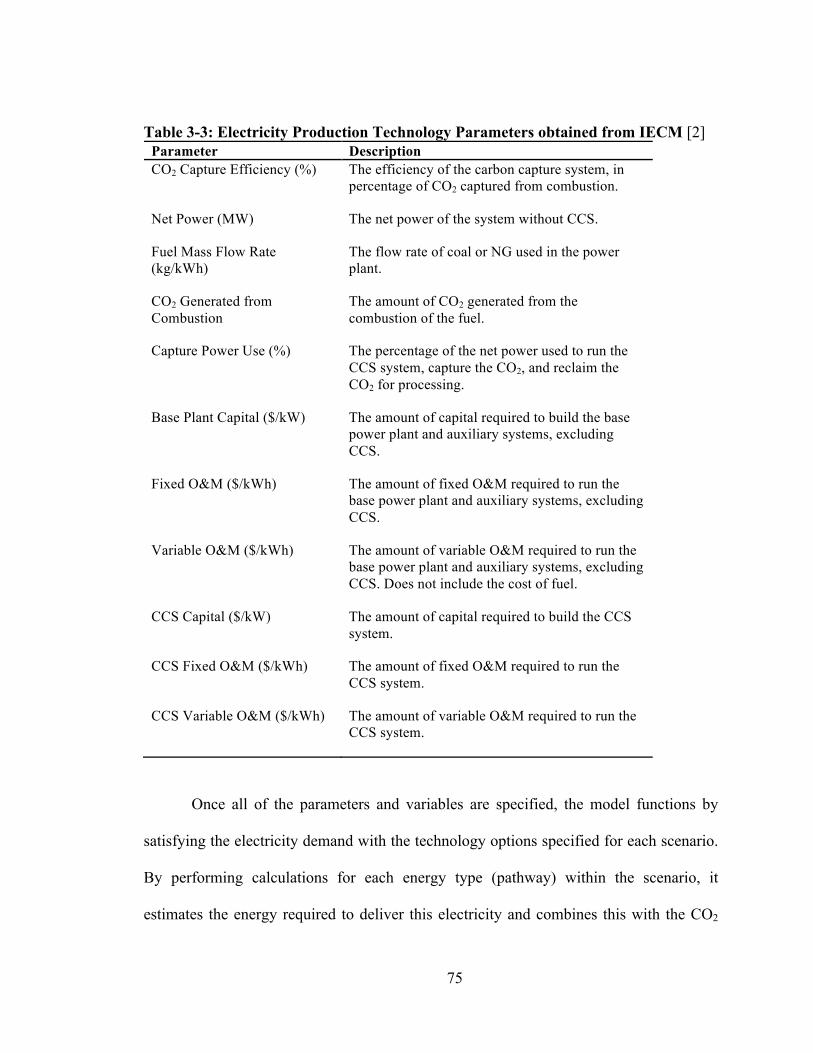
75

Table 3-3: Electricity Production Technology Parameters obtained from IECM [2] Parameter Description CO2 Capture Efficiency (%) The efficiency of the carbon capture system, in

percentage of CO2 captured from combustion.

Net Power (MW) The net power of the system without CCS.

Fuel Mass Flow Rate (kg/kWh)

The flow rate of coal or NG used in the power plant.

CO2 Generated from Combustion

The amount of CO2 generated from the combustion of the fuel.

Capture Power Use (%) The percentage of the net power used to run the CCS system, capture the CO2, and reclaim the CO2 for processing.

Base Plant Capital ($/kW) The amount of capital required to build the base power plant and auxiliary systems, excluding CCS.

Fixed O&M ($/kWh) The amount of fixed O&M required to run the base power plant and auxiliary systems, excluding CCS.

Variable O&M ($/kWh) The amount of variable O&M required to run the base power plant and auxiliary systems, excluding CCS. Does not include the cost of fuel.

CCS Capital ($/kW) The amount of capital required to build the CCS system.

CCS Fixed O&M ($/kWh) The amount of fixed O&M required to run the CCS system.

CCS Variable O&M ($/kWh) The amount of variable O&M required to run the CCS system.

Once all of the parameters and variables are specified, the model functions by

satisfying the electricity demand with the technology options specified for each scenario.

By performing calculations for each energy type (pathway) within the scenario, it

estimates the energy required to deliver this electricity and combines this with the CO2

76

emissions factors for each energy type and then sums across all pathways to estimate total

CO2 emissions. For example, the total CO2 emissions released by a plant in a given year

is the product of the emissions factor or energy specific emissions intensity (kilograms of

CO2 per kilowatt hour) by the total emissions produced by that plant in that year. In

plants with CCS, energy requirements of the CO2 capture and processing systems are

accounted for by subtracting a percentage of the net power without CCS. The impacts of

this parasitic power on fuel consumption and emissions intensity are also accounted for.

The emissions for each plant are summed across all plants in the system to estimate

system wide emissions for each scenario.

Costs in the model, and in the framework in general, are constant 2011 dollars.

The cost of electricity is calculated by levelizing the total capital requirement (TCR) and

the total fixed and variable O&M costs on a per kWh basis. These calculations result in

the Levelized Cost of Electricity (LCOE), which is the annual revenue requirement for

breakeven operation over a specified plant lifetime [18][37]. LCOE is calculated as

follows:

𝐿𝐶𝑂𝐸 =    𝐿𝐶𝐹 ∗ 𝐹𝑂𝑀 +  𝑉𝑂𝑀 + (𝑇𝐶𝑅 ∗ 𝐶𝐶𝐹 ∗ 𝐶𝑅𝐹)

𝑈 ∗ 8766 ∗ 𝑃!"#

where FOM represents the fixed O&M cost ($/year);

VOM represents the variable O&M cost ($/year);

TCR represents the total capital required ($);

LCF represents the levelized charge factor, which accounts for inflation and cost

escalations;

77

CCF represents the capital cost factor, which accounts for different capital costs in

different regions;

and CRF represents the capital recovery factor, which is the ratio of constant annuity to

the present value of the capital required. It is used to represent the value of the capital

required for the plant in annualized terms. The CRF is calculated as follows [38];

𝐶𝑅𝐹   =𝑖   1+ 𝑖 !

1+ 𝑖 ! − 1  

where i represents the incurred interest rate;

and n represents the compounding periods.

The model distinguishes between base plant costs and CCS costs. It also

distinguishes between retrofit and new build costs for CCS. Pipeline transport annualized

capital costs are treated as an O&M cost in the model, since transport and storage would

generally be purchased from a separate company and not part of the power plant [2].

2.3.2 Model Design and Relevant Equations

The MATLAB [1] model is divided into four main routines; plant specifications,

scenario creation, plant performance, and result culmination routines. Figure 3-4 provides

a reference overview of the general design and flow of information. Each routine

executes calculations for each year over the timeline specified. Deterministic results are

created and then passed on to the Uncertainty Assessment Model for further analysis.

78

Figure 3-4: MATLAB [1] Model Design Concept.

In the first routine, plant specifications are calculated based on raw data provided

from IECM [2] for plant characteristics. The goal of these calculations is to convert the

data from IECM [2] into energy specific values by dividing them by the total energy

generated by the plant in one year. They can then be used to calculate the cost and

emissions in the Plant Performance and Cost routine. The energy specific CO2 created

during combustion (kg/kWh), represented with 𝐺!"#$, and corrected for CCS parasitic

power requirements, is calculated as follows;

𝐺!"#$ =  𝛼 ∙ 𝑅!!" +  𝐺!"#$

where 𝑅!!", represents the percentage of the plants net power required for CCS system

operation (i.e., the parasitic power);

α represents the parasitic CCS power correction factor (kg/kWh) for the energy specific

CO2 (mass per kWh) created during combustion;

and 𝐺!"#$ represents the energy specific CO2 created during combustion for the plant

without CCS (kg/kWh).

79

The energy specific CO2 captured is calculated as follows:

𝐺!"# =  𝜂!"!×  𝐺!"#$

where  𝐺!"#  is  the  energy  specific  CO2  captured  (kg/kWh);

 𝜂!"!  is  the  CO2  capture  efficiency  (%);

and  𝐺!"#$  is  the  energy  specific  CO2  produced  during  combustion  of  the  fuel  (kg/kWh).

The energy specific net CO2 emitted, which is the difference between the CO2

captured and the CO2 created during combustion is calculated as follows;

𝐺!"# =    𝐺!"#$ −  𝐺!"#

where  𝐺!"#  is  the  energy  specific  net  CO2  emitted  (kg/kWh).

The net power capacity of an individual plant with CCS is calculated as follows;

𝑃!"# =    𝑃!"# −  𝑃!"# ∗ 𝑅!!"

where  𝑃!"#  represents  the  net  power  capacity  of  a  plant  with  CCS  (MW);

𝑃!"#  represents  the  net  power  capacity  of  a  plant  without  CCS  (MW);

and  𝑅!!"  represents  the  percentage  of  power  required  for  CCS  operations  (%).

The energy specific carbon tax is calculated as follow;

𝐶!"# =    𝑅!"# ∗  𝐺!"#

1000  𝑘𝑔/𝑡𝑜𝑛𝑛𝑒

where  𝐶!"#  represents  the  energy  specific  carbon  tax  ($/kWh);

and Rtax represents the mass specific (unit per unit mass) tax rate ($/t CO2).

The energy specific fuel rate (kg/kWh) of a plant with CCS, represented with 𝐹,

and corrected for CCS parasitic power use, is calculated with the following;

𝐹 =  𝛽 ∙ 𝑅!!" +  𝐹

80

where 𝐹 represents the energy specific fuel rate of the plant without CCS (kg/kWh),

and 𝛽 represents the parasitic CCS power correction factor (kg/kWh) for the energy

specific fuel rate.

The energy specific energy fuel cost is calculated as follows;

𝐶! =    𝐹! ∗  𝐹 ∗ 𝑄!"#$1000000

where  𝐶!  represents  the  energy  specific  fuel  cost  ($/kWh);

𝐹! represents the energy specific price of fuel ($/GJ);

𝐹 represents the energy specific fuel use of the plant (kg/kWh);

and  𝑄!"#$ represents the higher heating value of the fuel (kJ/kg).

Once the energy specific parameters have been calculated, the scenario routine

begins by taking the multi-year forecast for required electricity energy for the system, and

the set of user specified scenario requirements used for scenario creation (i.e., the fate of

specific technologies). The goal of this routine is to generate three variables for each

technology for each year; energy production share, total number of plants required, and

total generation capacity requirement. Here the forecasted energy requirement is divided

up into the respective electricity generation technologies mentioned above in Table 3-2,

based on the share for each technology. The scenario routine directs the fate of plant

technologies by using four user designated conditions based on the desired outcome;

retire, maintain, retrofit, and develop. Respective plant generation shares, plant capacities

required, and the numbers of plants required are calculated for each technology type with

the set of equations presented below, based on their assigned condition.

81

For the retire condition, plants are retired over a specified schedule, by directing

the number of plants that retire each year. The technology with this condition does not

experience growth in production share or number of plants. Total plant capacity (MW),

represented by 𝐷!,!, required to meet demand under the retire condition for each year y

and each technology type p is calculated as follows:

𝐷!,! =    𝑈! ∗ 𝑁!,! ∗  𝑃!"#!

where y represents the year;

p represents the plant technology type;

𝑈! represents the capacity factor or utilization of the plant (%);

𝑃!"#! represents the net power output of the plant (MW);

and 𝑁!,! represents the user specified number of plants in each year.

Electricity production share for each year is calculated as follows:

𝑋!,! =    𝐷!,!𝐷!!

where  𝑋!,!  is  the  production  share  (%)  in  each  year;

𝑎nd  𝐷!!  is the total capacity required to satisfy the demand for electricity in each year

provided in the forecast.

The maintain condition preserves the production share of the specified

technology, effectively allowing the number of plants with this property to increase but

only within the user specified share. Electricity production share, X, is constant and

provided. Required total capacity (MW), 𝐷!,!, is calculated as follows;

𝐷!,! =    𝑋!,! ∗ 𝐷!!

82

and the number of plants, 𝑁!,!, is a is calculated as follows:

𝑁!,! =  𝐷!,!

𝑈! ∗ 𝑃!"#!

For the develop condition, the production share of the technology increases based

on the share freed up by retiring plants in the system. Electricity production share is

calculated as follows;

𝑋!,! =    1− 𝑋!,!!,!

where, 𝑋!,! represents the production share for the other plant technologies.

The total capacity (MW) is calculated as follows:

𝐷!,! =    𝑋!,! ∗ 𝐷!!

and the number of plants, 𝑁!,!, is calculated as follows;

𝑁!,! =  𝐷!,!

𝑈! ∗ 𝑃!"#!

A retrofit condition is chosen for a technology for some future retrofit, such as

CCS or some other technological enhancement. It allows share growth in the pre-retrofit

host technology, calculated as follows:

𝑋!,! =    1− 𝑋!,!!,!

plant capacity required (MW), 𝐷!,!, is calculated as follows:

𝐷!,! =    𝑋!,! ∗ 𝐷!!

and the number of plants,  𝑁!,!, is a is calculated as follows:

83

𝑁!,! =  𝐷!,!

𝑈! ∗ 𝑃!"#!

until the specified year the retrofit begins, at which point the number of plants, 𝑁!,!, is

fixed (i.e., the number of plants in the system requiring retrofits at the time of the

technology introduction is a constant).

New plants that are built with the same technology used in the retrofitted plants

take over the growth of share from the host technology using the same equation as above,

along with the same capacity and number of plants equations. A retrofit period is

specified in number of years, where a retrofit rate is set for exiting plants to be retrofitted.

For plants that have been retrofitted, the retire condition is activated, meaning that 𝑁!,! is

dictated based on retrofit rate and the economic life of a retrofitted plant. These

retrofitted plants retire at the end of the given economic life.

The plant performance routine uses the yearly plant energy shares for each

technology (Xy,p), calculated in the scenario routine, to calculate the share of energy the

plant generates for each year. The goal of this routine is to use the electricity produced by

each technology to calculate the resulting cost and emissions. Additional variables for

fuel properties (cost, energy content, life cycle data), economic characteristics (carbon tax

and capital recovery factor), and plant performance (net power, capacity factor, capture

efficiency, cost data) are given as inputs along with the variables from the scenario

routine (X, N, D). It then calculates the electricity each technology type generates, with:

𝐸!,! =    𝑋!,! ∗  𝐸!!

where,  𝐸!,! is the share of the total electric energy generated by the technology type

(GWh);

84

and 𝐸!!, is the electric energy generated by the whole system (GWh) provided by the

energy forecast.

Cost and emissions results for each technology are then calculated by multiplying

the electricity produced in that year by the energy specific plant variables (emissions

intensity and levelized cost of electricity). The total CO2 released from the plant in a

given year (Mt CO2), represented by 𝐺!"#!,!, is calculated as follows:

𝐺!"!!,! =    𝐺!"#! ∗  𝐸!,!

The total GHG captured in a given year (Mt CO2), represented with  𝐺!"#!,!, is calculated

as follows:

𝐺!"#!,! =    𝐺!"#! ∗  𝐸!,!

The upstream GHG released from the extraction and transportation of fuel is

calculated by using the fuel consumed, and the intensity factor of the upstream emissions

(mass of GHG released per unit of fuel consumed). The energy specific upstream GHGs

emitted from fuel extraction and transportation (kg CO2e/kWh), represented as 𝐺!!, is

calculated with:

𝐺!! =    𝐹!! ∗  𝐹! ∗ 𝑄!"#$!

1000000

where the fuel mass energy specific GHG factor is 𝐹!! (kg/GJ);

𝐹!  is  the  energy  specific  fuel  use  of  the  plant  (kg/kWh);

and  𝑄!"#$!  is  the  higher  heating  value  of  the  fuel  (kJ/kg).

85

The total GHG emitted from fuel extraction and transportation in a given year (Mt CO2e),

represented as 𝐺!!,!, is calculated as follows:

𝐺!!,! =    𝐺!! ∗  𝐸!,!

1000000  𝑘𝑔/𝑀𝑡

The total life cycle GHG emitted (upstream and direct flue gas emissions) in a given year

(Mt CO2e), represented as 𝐺!!,!, is calculated as follows:

𝐺!!,! =    𝐺!!,! + 𝐺!"#!,!

The levelized cost of electricity for the plant, represented as 𝐿𝐶𝑂𝐸!, is calculated

with the following equation [18][37]:

𝐿𝐶𝑂𝐸! =    𝐿𝐶𝐹 ∗ 𝐹𝑂𝑀! +  𝑉𝑂𝑀! + (𝑇𝐶𝑅! ∗ 𝐶𝐶𝐹 ∗ 𝐶𝑅𝐹)

𝑈! ∗ 8766(ℎ𝑜𝑢𝑟𝑠𝑦𝑒𝑎𝑟 ) ∗ 𝑃!"#!

where, 𝐹𝑂𝑀!, is the fixed O&M cost ($/year);

𝑉𝑂𝑀!, is the variable O&M cost ($/year);

TCR is the total capital required ($);

LCF is the levelized charge factor, which accounts for inflation and cost escalations, is

set to 1 as default in this thesis to maintain constant dollars;

CRF is the capital recovery factor;

and CCF is the capital cost factor, which accounts for different capital costs in different

regions.

The final step, the result culmination routine, calculates desired outputs for cost

and environmental performance results by calculating the cumulative values (from year 1

86

to n). The total life cycle GHG emissions for all years simulated across the system, GTotal,

for each year y, and each plant p, is calculated with the following equation;

𝐺!"#$% =     𝐺!!,!!,!

The average Levelized Cost of Electricity, 𝐿𝐶𝑂𝐸, for the system over the

specified time frame is calculated with the following equation:

𝐿𝐶𝑂𝐸 =     (𝐿𝐶𝑂𝐸  !,!!,! ∗ 𝐸  !,!)

𝐸!!!

The cost of CO2 abatement, CCA, is the cost that is incurred by sequestering the

CO2 that would normally have been released into the atmosphere. It requires a reference

scenario and a scenario in which CO2 was captured. It is calculated as follows:

𝐶𝐶𝐴 =  𝐿𝐶𝑂𝐸!"# −  𝐿𝐶𝑂𝐸!"# ∗ 𝐸!!!  

𝐺!"#$%!"# − 𝐺!"#$%!"#

where 𝐿𝐶𝑂𝐸!"# represents the average levelized cost of electricity for the capture

scenario;

𝐿𝐶𝑂𝐸!"# represents the average levelized cost of electricity for the reference scenario;

𝐺!"#$%!"# represents the total life cycle GHG emissions for the capture scenario,

and  𝐺!"#$%!"# represents the total life cycle GHG emissions for the reference scenario.

2.4 Integration with the Uncertainty Assessment Model

The MATLAB [1] model presented here is designed to interface with the

Uncertainty Assessment Model presented in Section 3, below. Access to the inputs and

outputs of the Integrated Life Cycle Model is required for full functionality of the

87

uncertainty aspect of the framework to allow for the sensitivity and uncertainty analysis

methods described below.

3 Uncertainty Assessment Model for Evaluating Advanced CCS Technologies

3.1 Introduction

Uncertainty analysis provides additional data for decision-makers to consider

when looking at investment, policy making, and technology adoption. It is difficult to

assess the LC impacts of developing energy technologies due to limited data regarding

actual performance and the cost of new technologies. The data that is available is

typically of reduced quality compared to those technologies that have already been

implemented at a commercial scale. There is a greater uncertainty associated with actual

performance and cost of new technologies when implemented at a commercial scale. This

uncertainty in turn increases the variability and uncertainty of the potential environmental

impacts of the technology. By explicitly addressing uncertainty, researchers are able to

model future scenarios and create more robust conclusions about the use of advanced

technology.

3.2 Method

The uncertainty assessment model proposed here, depicted schematically in

Figure 3-5, incorporates a set of methods to aid CCS technology researchers in defining

and quantifying the uncertainty. It provides a numerical means to assess uncertainty,

which in turn may have an impact on selected use of the resultant data by decision-

makers. The results provided from the previously defined integrated life cycle model can

be assessed in relative terms, such as a comparison to competing alternatives (i.e.,

88

scenario based) or through absolute means (i.e., target based). The use of this uncertainty

assessment model with the integrated life-cycle model will help to determine the trade-

offs between different technology options and the environmental and cost effects of

decisions about technology options.

The Uncertainty Assessment Model (UAM) will help to determine data

collection needs, predominant parameters that require additional analyses, the

quantification of probability distributions for the results (rather than point estimates or

ranges), and the conditions that could change the result rankings. To achieve this, the

uncertainty assessment model contains two main elements, 1) a sensitivity analysis and 2)

an uncertainty analysis that quantifies the uncertainty within the study. The following

section of this chapter will describe the various components of the UAM, how these

components use the information provided by the integrated life-cycle model, and finally

define the roles of the components in providing relevant information to decision makers.

89

Figure 3-5: Uncertainty Assessment Model and Resulting Output

3.2.1 Deterministic Sensitivity Analysis

A structured deterministic sensitivity analysis is proposed to expose important

parameters that make the largest contribution to the overall uncertainty in the results. This

is achieved by assessing the sensitivity of deterministic results to variation in technology

and system parameters used within the Integrated LC Model. In it, two numerical

methods are employed, a contribution analysis and a perturbation analysis.

3.2.1.1 Contribution Analysis

90

A Contribution Analysis [39] breaks down the results into the contributions that

systems components make toward the total. It is proposed to provide a breakdown of the

electricity production system’s contributors (i.e., generation technology) in terms of

emissions and costs [39]. The goal of this analysis is to provide a general overview of the

whole system and highlight the largest contributors to inform further analyses. For

example, the largest contributors have larger relative influence on the results, and this

information can lead to further analysis by focusing on these contributors. The

Contribution Analysis [39] functions in this thesis by calculating the contributions that

each electricity generation technology (i.e., specific plant types) makes toward the total

cost and LC emissions output, and also the contribution that each emissions path (i.e.,

captured, upstream, and stack emissions) makes toward the total LC emissions output.

3.2.1.2 Perturbation Analysis

A Perturbation Analysis [39] determines the effect of variability in single

parameter values on the overall result. The parameter values are individually varied by a

marginal amount while observing the resulting change in model output. The two goals of

this analysis are to rank the parameters according to their influence on the results and to

generate information about these parameters (magnitude of influence) to inform the

researcher about the implications of data inaccuracy. A sensitivity ratio, represented by

SR, for each parameter is calculated using the following [39]:

𝑆𝑅 =  

𝑌! − 𝑌!𝑌!

𝑋! − 𝑋!𝑋!

where 𝑌! represents the result after the perturbation;

91

𝑌! represents the result prior to perturbation;

𝑋! represents the parameter value after perturbation;

and 𝑋! represents the parameter value prior to perturbation.

Parameters are ranked based on their relative influence (i.e., higher SRs denote

higher relative influence), which provides the researcher with a means of focusing further

analyses on the most important parameters.

3.2.2 Uncertainty Analysis

Upon completion of the deterministic sensitivity analysis, and using the resulting

list of important parameters found through the perturbation analysis, uncertainty in the

results is quantified through uncertainty propagation. Uncertainty in important parameters

is represented with probability distributions that are specified based on available

information (i.e., existing experimental data, studies, and expert judgment). A MCS [40]

is used to estimate the magnitude of uncertainty in the results by propagating the

uncertainty of various inputs to the full set of results. Uncertainty in the results for all of

the scenarios is represented with histograms, and further analyzed with a Discernibility

Analysis [39].

3.2.2.1 Distribution Type Selection

Choice of input probability distribution is critical to the robustness of the results

since the resulting probability distributions of the outcomes are ultimately formed from

the inputs. Unfortunately, a lack of data for emerging CCS technology parameters is a

concern. Methods for representing input uncertainty include fuzzy sets (e.g., [41][42]),

min-max intervals (e.g., [43]), and probability distributions (e.g., [44]). This study

92

focuses on the use of a set of probability distribution types that represent a range of

values for specific parameters, with a sensitivity analysis performed (see Section 3.2.3.1

for details) to determine the effect of the probability distribution type on the MCS results.

3.2.2.2 Uncertainty Propagation

Once appropriate distributions are selected for the input parameters, they can be

sampled from and run through the Integrated LC Model discussed in Section 2 of this

Chapter. The method chosen for this task is a Monte Carlo Simulation [40] sampling

method. While a Latin Hypercube [45] scheme would be beneficial in this analysis (i.e.,

efficiency through a reduction of samples required), a large number of samples (on the

order of 10000) are used in all simulations. This large number is assumed to be sufficient

to cover the full range of distributions used based on sample sizes used in existing studies

(e.g., [18][46-49]).

3.2.2.3 Discernibility Analysis

The goal of a Discernibility Analysis [39] is to resolve the differences between

individual scenario probability distributions (i.e., the probability that one scenario will

prevail over another or will meet a target) obtained from the Uncertainty Propagation

Analysis. The resolved differences are used to rank the scenarios and, effectively reduce

the information provided in the results (i.e., probabilities assigned to values) down to a

single metric [39]. Figure 3-6 provides an example of two different scenarios and the

use of this analysis. Probability distributions are shown for Scenario 1 and 2 in Figure

3-6a, with corresponding values for percent of the distribution area outside of the

alternate scenario, X and Y respectively. The results from this analysis are presented in

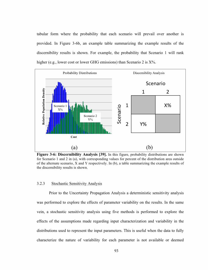
93

tabular form where the probability that each scenario will prevail over another is

provided. In Figure 3-6b, an example table summarizing the example results of the

discernibility results is shown. For example, the probability that Scenario 1 will rank

higher (e.g., lower cost or lower GHG emissions) than Scenario 2 is X%.

Figure 3-6: Discernibility Analysis [39]. In this figure, probability distributions are shown for Scenario 1 and 2 in (a), with corresponding values for percent of the distribution area outside of the alternate scenario, X and Y respectively. In (b), a table summarizing the example results of the discernibility results is shown.

3.2.3 Stochastic Sensitivity Analysis

Prior to the Uncertainty Propagation Analysis a deterministic sensitivity analysis

was performed to explore the effects of parameter variability on the results. In the same

vein, a stochastic sensitivity analysis using five methods is performed to explore the

effects of the assumptions made regarding input characterization and variability in the

distributions used to represent the input parameters. This is useful when the data to fully

characterize the nature of variability for each parameter is not available or deemed

94

unreliable. The purpose of this analysis is to gain an understanding of the effects that

parameter representation uncertainty has on the results by observing the conditions that

force a change in scenario rank or a change in the statistical confidence level against

some target.

3.2.3.1 Probability Distribution Scenario Analysis

In some cases data regarding the nature of a parameter’s distribution over a given

range is sparse or the future value or behaviour of the parameter over a long time period

is difficult to predict. A Scenario Analysis can be useful to create states to characterize

the uncertainty in parameter ranges and allow for a sensitivity analysis regarding these

states to be conducted. A Probability Distribution Scenario Analysis achieves this same

goal by defining the nature of the parameter distribution characteristics. For example, as

demonstrated in Figure 3-7, the variability in long-term price estimates of natural gas can

be defined within a range of values, while the stability can be defined using a probability

distribution that reflects the characteristics of the stability. A more stable price of NG

over a time period would have a probability distribution with a smaller standard deviation

(σStable in Figure 3-7), while a less stable price distribution would have larger standard

deviations (σUnstable in Figure 3-7). In addition, skewness in the underlying parameter

distributions used to form the scenarios can be used to represent bias in estimates, such as

a bias toward higher or lower long-term NG Prices. Using this form of scenario analysis

in conjunction with the Uncertainty Propagation Analysis can allow the researcher to

examine various scenarios to determine its effect on outcomes such as GHG emissions or

LC cost.

95

Figure 3-7: Probability Distribution Sensitivity Analysis Example using NG Price Stability. In this figure, probability distributions are shown for stable and unstable NG Price distributions representing the uncertainty in long term NG Prices.

3.2.3.2 Probability Distribution Type Sensitivity Analysis

In this method, a sensitivity analysis is completed when data on the shape of the

probability distribution is not fully understood. The goal in this method is to determine

the overall effect of imperfect representation of the inputs on the results through a change

in scenario ranking. A base case, or the initial selection of distribution types based on

available data or expert judgment, is compared to cases where all parameters are

represented with uniform, triangular, and beta distributions. The analysis then compares

the resultant distributions for each scenario, allowing for inspection of the effects that the

different types of distribution shapes have on the original results.

3.2.3.3 Relative Degree of Optimism Analysis

In a situation where data regarding the bias of the variability in underlying

parameter distributions is not available, there is a degree of uncertainty in choosing the

Relative  Population  Density  

NG  Price  ($/GJ)  

Stable  

Unstable  

σStable  <  σUnstable

96

appropriate shape of probability distributions used to represent inputs. This has the

potential to misleading conclusions [50]. The skewness, or extremal tendency of the

inputs may not be represented correctly, resulting in distributions that are too optimistic

or pessimistic in representing the probability that the values will tend to one extreme or

the other. A test is proposed to explore how susceptible the results are to skewness in the

underlying parameter distributions’ assumptions. The method used here, called the

Relative Degree of Optimism Analysis, is performed by first representing the parameter

inputs as beta distributions using the beta probability function to represent the variability.

A parameter value, represented here as p, is calculated with the following:

𝑝 = 𝐿! + 𝑃𝐷𝐹!"#$(𝐿! − 𝐿!)

where Ll represents the lower limit of the parameter range;

Lu represents the upper limit of the parameter range;

and PDFBeta represents the beta probability distribution function, calculated as follows:

𝑃𝐷𝐹!"#$ =  𝑥!!! 1 − 𝑥 !!!

𝐵 𝛼,𝛽

where α  and  β are parameters that control the shape of the resulting distribution curve;

and B(α,β) is the beta function [51]. The shape parameters are iteratively changed, as

demonstrated in Figure 3-8, to skew the input distributions from the pessimistic lower

range limit (Ll) with α values greater than β values, to the optimistic upper (Lu) with β

values greater than α.

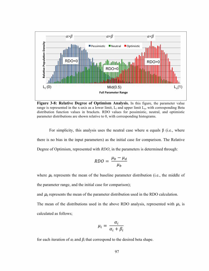
97

Figure 3-8: Relative Degree of Optimism Analysis. In this figure, the parameter value range is represented in the x-axis as a lower limit, Ll and upper limit Lu, with corresponding Beta distribution function values in brackets. RDO values for pessimistic, neutral, and optimistic parameter distributions are shown relative to 0, with corresponding histograms.

For simplicity, this analysis uses the neutral case where α equals β (i.e., where

there is no bias in the input parameters) as the initial case for comparison. The Relative

Degree of Optimism, represented with RDO, in the parameters is determined through:

𝑅𝐷𝑂 =  𝜇! − 𝜇!𝜇!

where μb represents the mean of the baseline parameter distribution (i.e., the middle of

the parameter range, and the initial case for comparison);

and μd represents the mean of the parameter distribution used in the RDO calculation.

The mean of the distributions used in the above RDO analysis, represented with μi, is

calculated as follows;

𝜇! =  𝛼!

𝛼! + 𝛽!

for each iteration of αi  and  βi  that correspond to the desired beta shape.

α>β α=β α<β

98

This results in estimates of the degree to which the distribution is skewed to either side of

the range mid-point. For example, a RDO value of zero (green distribution in Figure 3-8)

denotes a neutral distribution situation, while an RDO>0 (red distribution in Figure 3-8)

denotes an optimistic distribution situation (i.e., skewed to the lower end of the cost

range, and higher end of the performance range). A RDO<0 denotes a pessimistic

situation (blue distribution in Figure 3-8). Subsequent result distributions for each RDO

iteration are recorded, and when used in conjunction with a Discernibility Analysis,

allows for a relationship between the RDO and the confidence level in ranking one option

higher than a competing alternative to be drawn. In this way, a sense of how bias in input

parameters affects the outcome can be provided. This can be useful in determining the

improvement in technology cost and performance to meet targets or to rank higher than

an alternative.

3.2.3.4 Technology Availability and Improvement Analysis

Information regarding the possible improvement in technology cost and

performance over time may not be available, but can be estimated using learning curves

(e.g., [20]). Learning curves, or experience curves, are an expression of learning with

experience [52]. The basis of this idea is that with the accumulation of experience using a

technology, the technology will become cheaper. However, learning curves are subject to

uncertainty in the amount of capacity built over time and the learning rates selected for a

particular technology [53]. When looking at long range projections of advanced CCS

technology use, it may be useful to represent a linkage in improvement in technology cost

and performance to the time of technology introduction while incorporating the aspects of

the uncertainty propagation method proposed in this chapter. In this stochastic sensitivity

99

analysis, a method to assess the variability in technology improvement over time is

proposed. As with the RDO analysis presented above, beta distributions are used to

represent the input parameters within the specified range used in the previous analyses.

However, in this case the availability of the technology is linked through an inverse

relationship such that early technology availability results in cost and performance

parameter distributions that exhibit a bias towards the least attractive end of their

respective range (i.e., early introduction results in higher cost and worse performance). In

an iterative procedure, as demonstrated in Figure 3-9, the availability parameter

distribution shape is changed from having a bias to the lower range limit (i.e., early

availability, Figure 3-9a) with higher cost (Figure 3-9b) and lower performance (Figure

3-9c) to the higher range limit (i.e., late availability, Figure 3-9d), while the respective

cost (Figure 3-9e) and performance (Figure 3-9f) parameters distributions are changed in

step.

Figure 3-9: Technology Improvement Analysis. This analysis simulates the improvement in technology cost and performance within a specified range of values using beta distributions for parameter representation. As the availability of the technology tends toward the higher end (from (a) to (d)), the cost of the technology will tend toward the lower end of the range (from (b) to (e)), and the performance will tend toward the higher end of the range (from (c) to (f)).

100

Here it is assumed that the cost of the technology will tend toward the lower end

of the range, and the performance will tend toward the higher end of the range as the

availability of the technology tends toward the higher end [52]. For simplicity, this

analysis uses a linear relationship. A MCS is used to sample from the distributions for

each iteration, with subsequent resulting distributions recorded for each iteration. With

the use of Discernibility Analysis, the distributions are resolved into respective

probabilities associated to ranking higher (e.g., being lower in cost) than alternative

scenarios.

3.2.3.5 Combined Sensitivity and Uncertainty Propagation Analysis

A combined sensitivity analysis reveals the favourable conditions, based on two

parameters, in which a scenario outperforms alternative scenarios [54]. This thesis

proposes a Combined Sensitivity and Uncertainty Propagation Analysis that does this as

well, but improves on it by capturing the stochastic nature of the other input parameters.

An example is provided in Figure 3-10 for illustrative purposes. Two chosen parameters,

x and y in Figure 3-10 (e.g., for cost of electricity, the parameters could be carbon tax and

NG price), are varied simultaneously in a deterministic manner while other inputs are

represented using probability distributions. Using this method, a Monte Carlo Simulation

(MCS) is run for each change in the selected two parameters, generating a probability

distribution for each scenario (green and blue in Figure 3-10). The probability

distributions are analyzed and compared for each point (xi and yj in Figure 3-10), with the

most favourable scenario (e.g., in the case of cost, the least costly scenario) presented as

having the highest ranking in a gradient contour chart against the two parameters. The

101

distributions can be compared in a variety of ways, such as through the expected value

(i.e., probability distribution mean value) or through statistical significance. For

simplicity, this analysis uses the least expected value for the criteria to choose the

winning scenario.

Figure 3-10: Combined Sensitivity and Uncertainty Propagation Analysis Example. In (a), the cost probability results of two scenarios are shown for parameter values xi and yj, with Scenario 1 showing a higher probability of being the least cost option. In (b) the results of several distributions like in (a) are shown in a contour plot with x and y representing the chosen parameters. Here the colour of the plot designates the favourable scenario and the corresponding value for x and y required for favourability.

3.3 Combination with the Integrated Life Cycle Model

The Uncertainty Assessment Model presented here works by systematically and

repeatedly manipulating the input parameters used by the Integrated Life Cycle Model

and observing the results produced. The deterministic sensitivity analyses, presented in

Section 3.2.1, manipulate the input parameters in a one-at-a-time manner. They operate

by changing the specific parameters individually and rerunning the MATLAB [1]

102

routines represented in Figure 3-4 for each parameter in question. The uncertainty

analysis methods in Section 3.2.2 and the stochastic sensitivity analyses in Section 3.2.3

use a multiple parameter manipulation method, where the sampling of multiple

probability distributions for all parameters in question provides a unique set of values for

each MCS sampling. The operation of the MATLAB [1] routines, represented in Figure

3-4, is executed for each MCS run, producing results equal to the number of samples

taken, allowing for the creation of a histogram result.

4 Case Study Formulation

4.1 Alberta’s Future Electric System Pathways

In Chapter 1 the justification was made for using Alberta for the case study based

on the challenges presented in choosing electricity production technologies to meet future

Albertan requirements. Alberta has large fossil fuel energy resources available for use in

electricity production. However, developing these resources without considering GHG

emissions would have detrimental consequences to the environment. Alberta is under

pressure to meet increasing demand for electricity while contributing to GHG emissions

reduction initiatives and satisfying existing and future GHG policies.

There are several paths that can be taken, such as renewable energy technologies,

increasing NG technology share, and NG and coal technologies with CCS. However,

because fossil fuels are likely to be further exploited in Alberta, CCS incorporated with

thermal power generation is a leading option. As suggested in Chapter 1, there are two

prominent fossil fuel pathways for future development in Albertan power generation:

coal and NG. The first pathway is the use of clean coal technologies (i.e., SPCS, USCPC,

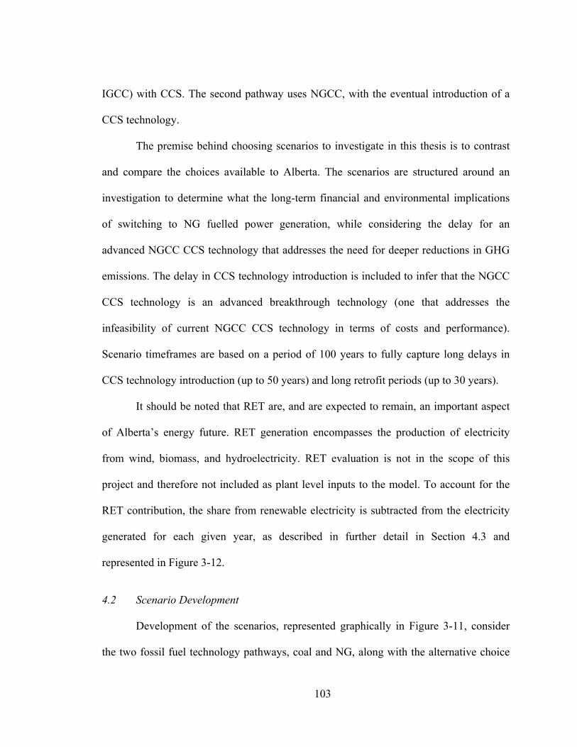
103

IGCC) with CCS. The second pathway uses NGCC, with the eventual introduction of a

CCS technology.

The premise behind choosing scenarios to investigate in this thesis is to contrast

and compare the choices available to Alberta. The scenarios are structured around an

investigation to determine what the long-term financial and environmental implications

of switching to NG fuelled power generation, while considering the delay for an

advanced NGCC CCS technology that addresses the need for deeper reductions in GHG

emissions. The delay in CCS technology introduction is included to infer that the NGCC

CCS technology is an advanced breakthrough technology (one that addresses the

infeasibility of current NGCC CCS technology in terms of costs and performance).

Scenario timeframes are based on a period of 100 years to fully capture long delays in

CCS technology introduction (up to 50 years) and long retrofit periods (up to 30 years).

It should be noted that RET are, and are expected to remain, an important aspect

of Alberta’s energy future. RET generation encompasses the production of electricity

from wind, biomass, and hydroelectricity. RET evaluation is not in the scope of this

project and therefore not included as plant level inputs to the model. To account for the

RET contribution, the share from renewable electricity is subtracted from the electricity

generated for each given year, as described in further detail in Section 4.3 and

represented in Figure 3-12.

4.2 Scenario Development

Development of the scenarios, represented graphically in Figure 3-11, consider

the two fossil fuel technology pathways, coal and NG, along with the alternative choice

104

of maintaining the status quo. A base case scenario was developed to represent the status

quo (red in Figure 3-11), where coal remains the primary fuel and NG plays a secondary

role. While this scenario is very unlikely, it is used as a baseline case that allows

measurement of the level of impact from the other scenarios. Two scenarios were

developed to represent the process of switching from coal to NG, one where no CCS is

adopted (blue in Figure 3-11), and another where an advanced breakthrough CCS is

adopted at some uncertain future time (black in Figure 3-11). The final scenario is one

where coal with a current CCS technology is the primary generation technology (green in

Figure 3-11), and NG is phased out, with the exception of cogeneration and peaking

units.

Figure 3-11: The choices considered for Alberta’s Future Electric System. Four scenarios were chosen to be investigated in this thesis, one base case, one where NG is the primary fuel, one where NG is the primary fuel but has CCS, and one where coal is the primary fuel but has CCS.

Each of the four scenarios in the case study are defined by the mix of electricity

production shares for each type of power generation technology used in Alberta on a

yearly basis, summarized in Table 3-4 with initial and final year shares. Two NG

technology shares are common among all scenarios. Cogeneration, used in the oil sands

sector due to the requirement for thermal energy, and NGSC, used for peak load

105

demands, are not expected to be replaced in the near to medium term, and are therefore

maintained in the scenarios. They maintain a share of 25% and 5% respectively. These

technologies. The scenarios take into account in-queue generation capacity additions (i.e.,

projects currently in construction, such as Keephills 34 and Shepard Energy Centre5) in

the simulation.

Table 3-4: Initial and Final Electricity Energy Production Technology Shares for All Scenarios

Production  Technology  

Initial  Year   Final  Year  (100  Years)  

All  Scenarios  

S1  

Base  Case  

S2  

NGCC  

S3  

NGCC  CCS  

S4  

SCPC  CCS  

PC   60%   0%   0%   0%   0%  

SCPC   5%   65%   0%   0%   0%  

SCPC  with  CCS   0%   0%   0%   0%   70%  

Cogeneration   25%   25%   25%   25%   25%  

NGSC   5%   5%   5%   5%   5%  

NGCC   5%   5%   70%   0%   0%  

NGCC  with  CCS   0%   0%   0%   70%   0%  

4.2.1 Scenario 1 - Base Case

The base case Scenario 1 (represented as S1 in Table 3-4) assumes that no GHG

mitigation is undertaken, while the production shares of Alberta’s current power

generation technology mix are maintained into the future with the exception of PC. For

4 The Keephills 3 power plant is a 495 gross MW (450 MW net) SCPC generating facility that began operation in September 2011. [55]

5 The Shepard Energy Centre is an 800 gross MW NGCC generation facility with planned completion in 2015. [56]

106

coal, the dominant technology for electricity generation is initially PC (60% of the share),

while all new coal plants are assumed to use more advanced SCPC. For NG, the

dominant technology for electricity generation is cogeneration (25% of the share)

followed by NGCC (5% of the share) and NGSC (5% of the share). The state of this

scenario at the end of 100 years is that SCPC has 65% of the share, while NG

technologies make up the remaining 35%.

4.2.2 Scenario 2 - NGCC

Scenario 2 (represented as S2 in Table 3-4) is intended to represent a situation

where NG displaces coal as the primary fuel source for electricity generation, with no

GHG mitigation technology. This is a plausible scenario since low NG price forecasts,

lower capital costs of NGCC plants, and incoming Canadian Federal GHG regulations

make NGCC economically and environmentally attractive. In this scenario, both existing

PC and SCPC plants are retired based on their retirement schedules6 within thirty years

(0% share). Cogeneration and NGSC shares are maintained, while growth in demand is

met by building new NGCC plants, which results in a share of 75% at the end of the 100

years.

4.2.3 Scenario 3 - NGCC with Advanced CCS

Scenario (represented as S3 in Table 3-4) is identical to S2 except that an

improved CCS technology is introduced for NGCC plants at some future time. At that

point, existing NGCC plants are retrofitted with the advanced CCS technology and

6 Expectations set by Environment Canada’s Coal Emissions Regulations [57] imply that over 1000 MW of coal generation will retire prior to 2020, with an additional 3000 MW between 2021 and 2029. [6]

107

growth in demand is met by building new NGCC plants with CCS. This scenario

represents the advanced CCS technology by modeling one that is improved in cost and

performance up to 25% relative to existing estimates based on literature values (e.g.,

[2][31][58-64]), with the uncertainty in this technology represented using a range of

values for various parameters discussed in Section 4.4 below. The end state of this

scenario is that NGCC with CCS has 70% of the share at the end of 100 years.

4.2.4 Scenario 4 - SCPC with CCS

In this scenario (represented as S4 in Table 3-4), NGCC and PC plants are phased

out with assumed retirement schedules and expected life times of 30 years [6] and growth

in demand is met by building new SCPC plants. A current amine CCS technology is

introduced in the near term (five years) with SCPC plants, resulting in a SCPC share of

70% at the end of 100 years. As with the other scenarios, cogeneration and NGSC shares

are maintained.

4.3 Forecast Energy Production

The electricity demand forecast used in this case study, shown as a black line in

Figure 3-12, is based on the forecast used in the 2012 AESO LTTP [6]. The AESO report

forecasts internal load out to 2029 (blue line in Figure 3-12), and uses a growth rate of

2.2% per year past 2025. This case study uses the AESO forecast out to 2029, and past

this point uses a linear growth rate of 2.9 TWh per year (represented as a red line in

Figure 3-12, based on the slope of the AESO forecast at 2029) out to the year 2110. The

NG and coal portion is 90% of the total energy required based on 2011 AESO statistics

108

[6], and is the portion that is modelled within the framework. The remaining 10% of the

total energy demand is the renewable energy portion.

Figure 3-12: Long-term Electricity Energy Forecast for Alberta. The AESO forecast uses a 2.2% growth rate until 2029, after this year this study uses a linear growth rate of 2.9 TWh/year. Only the non-renewable portion of the forecast is modeled, while wind, hydro, and other sources of energy are taken off the total energy produced.

4.4 Key Parameter Descriptions and Range Assumptions

Within this case study there are twelve key parameters chosen for exploration in

the uncertainty analysis. The parameters are categorized into two groups, technology and

system parameters. While it can be argued that there are uncertainties in all parameters

used within the model, there are some that are considered much more uncertain and

therefore prime candidates for analysis. It is these that are of the greatest interest to this

study. A description of each follows, with a discussion regarding the assumptions used to

determine the range of values used to represent the uncertainty in this study.

109

The eight technology parameters considered in this thesis are those that are linked

to specific NGCC and NGCC CCS technologies. The first is the Availability Time of the

Advanced CCS Technology, or the introduction time in years from year zero, of an

advanced CCS technology for use with NGCC plants. This parameter is included to

explore the effect of introducing the technology at various times in the timeline. There is

little indication as to when the earliest available time would be for this technology. It is

assumed in this thesis that the earliest possible time would be ten years from year zero

(two years of R&D, five years for pilot project exploration, and three years to build the

first full size plant), with the latest time fifty years in the future.

The second is the Retrofit Period, which is the time in years that it takes to

retrofit all existing NGCC plants with CCS. The parameter is included to explore the

effect of different retrofit rates of the advanced technology for existing plants. An

assumption is made that between ten and thirty years would be sufficient.

The third is the Carbon Capture and Processing Parasitic Power. This is the power

required to run the CCS system, including all the pumps, compressors, and other

mechanical systems. It also includes the thermal energy to reclaim the CO2 from the

amine solution. This comes in the form of steam, which would have normally been used

in the steam turbine to generate electricity. This parameter is included for exploration to

study the effect of uncertainty in the impact of power requirements for the technology.

The range for this parameter, as described in Figure 3-13, is based on the average of

values obtained from studies assessing NGCC with CCS [31][58-64]. Here the average of

the survey range (represented as a black bar in Figure 3-13) is considered the maximum

110

of the case study range (represented as a red bar in Figure 3-13) at 14.7%, while a 25%

reduction in parasitic power is considered the minimum of the range at 11%.

Figure 3-13: Range of Values used for the Carbon Capture and Processing Parasitic Power Parameter. Here the average of the survey at 14.7% is considered the maximum of the range, while a 25% improvement in power requirements is considered the minimum of the range at 11% [31][58-64].

The fourth parameter is the CO2 Removal Efficiency of the capture system, which

is the rate of capture from the flue gas. Here, the impact of the uncertainty in the capture

performance of the technology is assessed. All studies surveyed [31][58-64] assumed

90% efficiency for capture. The range of values used in this thesis was based on an

improvement in efficiency of 2.5%, resulting in 92.5% efficiency for the maximum and

90% for the minimum.

The fifth parameter is the Capacity Factor of NGCC power plants. This is the

percentage of time that all NGCC plants (with and without CCS) operate in a given year.

The uncertainty in the actual use of NGCC is explored here, since it is possible that

NGCC plants may operate at less than baseload conditions. The range of values used in

this thesis, depicted in Figure 3-14, is based on the minimum of values used in studies

surveyed [31][58-64], at 40%, and the maximum set at a value of 90%, or equal to that of

a SCPC plant in this thesis.

Thesis  Range Survey  Range

111

Figure 3-14: Range of Values used for the Capacity Factor for NGCC Plants. Here the average of the survey is 75%, the minimum of the survey and of this study is 40%, while the maximum of the survey is 87% [31][58-64]. The maximum considered in this study is 90%.

The sixth parameter is the Capital Costs for the CCS system. These are the extra

capital costs (those above base plant costs) associated with the CCS system on an NGCC

plant. Here, the impact of the uncertainty in the capital costs of including CCS with

NGCC is explored. Values for the range of capital costs are derived from the survey

values [31][58-64], depicted in Figure 3-15. The range maximum is the average of the

study values at $623/kWnet. The minimum is based on a 25% improvement in capital

cost at $467/kWnet.

Figure 3-15: Range of Values used for the Capital Cost of CCS for NGCC Plants. Here the average of the survey is 623 $/kWnet, the minimum is 570 $/kWnet, while the maximum is 783 $/kW [31][58-64]. The minimum considered in this study is 467 $/kWnet, while the maximum of this study is 623 $/kWnet.

The seventh technology parameter is the Variable Operation and Maintenance

(O&M) costs for CCS. These costs include the sorbent (amine) and other chemical

resupply, and the transportation and storage costs associated with the CO2. The surveyed

Thesis  Range Survey  Range

Thesis  Range Survey  Range

112

studies did not provide specific information regarding the variable O&M costs other than

for the transportation and storage costs, which ranged from 2.9 to 7 dollars per tonne

[31][58-64]. IECM [2] provides a breakdown of the costs, and it is this value that is used

for the upper range of this thesis’ Variable O&M cost parameter at $6.69/MWh [2].

Again, a 25% improvement in cost is used as the lower end of the range, at $5.22/MWh.

The last and eighth technology parameter is the Retrofit Capital Penalty, which is

a factor that accounts for the additional cost of retrofitting an existing plant with a CCS

technology. It is applied to the capital cost of the CCS technology, rather than the capital

cost of the whole plant. Since existing plants may not have been built with a future

retrofit in mind, additional cost to modify the plant to accommodate the retrofit may be

required [65][66]. A range from 1 to 2 is used in this study to cover a range of penalty

factors [65][66].

System parameters are characterized as those that affect the entire generation

system. The first is the Price of Natural Gas. As mentioned earlier, the price of NG is

relatively unstable compared to coal when looking at historical values [16]. Based on the

history, a wide range of values is possible over the next several decades, as demonstrated

in Figure 3-16.

113

Figure 3-16: Henry Hub Gulf Coast Natural Gas Price 1997-2012. The unstable nature of NG prices from 1997-2012, with the wide range of just over $2/GJ to just under $10/GJ. [16]

The inclusion of this parameter in the uncertainty assessment allows for the

exploration of the impact of this NG price instability on the results. Ranges in other

studies have been centred on seven dollars per gigajoule [31][58-64]. This study uses a

wide range to cover the possibility of very high or low gas prices, based on the past

history as demonstrated in Figure 3-16. A low of $3/GJ to a high of $10/GJ is used, as

shown in Figure 3-17.

Figure 3-17: Range of Values used for the Price of NG. The average of the survey is $7.1 /GJ, the minimum is $6.9/GJ, while the maximum is $7.4/GJ [31][58-64]. The minimum considered in this study is $3/GJ, while the maximum is $10/GJ.

The second system parameter is the Carbon Tax imposed on the system. The

purpose of a carbon tax is to level the playing field amongst generation technologies, and

encourage electricity producers to choose less GHG emissive technologies. In a sense,

Thesis  Range Survey  Range

114

Carbon Tax is a tool used to influence the system, and as such it is not included in all of

the uncertainty assessment in this thesis since it would not make for informative results.

The analysis used in the case study uses an approach for carbon tax that allows for an

analysis of a wide range of values, and as such does not include the Alberta SGER tax.

Carbon tax is included in the analysis with the use of a Combined Sensitivity and

Uncertainty Propagation Analysis, discussed in more detail in the Section 2.3.5 of

Chapter 4.

The third system parameter is the Capital Recovery Factor (CRF), also known as

the Fixed Charge Factor (FCF) in other studies (e.g., [18]). It reflects the assumed cost of

capital for a project over a specified amortization period. This factor is used uniformly in

all capital cost calculations for the entire system. The survey results, represented in

Figure 3-18, show a wide range of values used [31][58-64]. The average of this range,

and the range maximum used for this thesis, is 13 percent while the minimum for both is

11 percent.

Figure 3-18: Range of Values used for the Capital Recovery Factor. The average of the survey is 13%, the minimum is 11%, while the maximum is 18%. The minimum considered in this study is 11%, while the maximum is 13% [31][58-64].

Finally, the fourth system parameter is the Life Cycle Emissions of NG Extraction

and Transportation. This parameter is included to assess the impact that potentially high

emissions from the extraction, processing, and transportation of NG may have on the

Thesis  Range Survey  Range

115

overall results. In a study by the US National Energy Technology Laboratory (NETL) on

the role of alternative energy sources [17], the value of GHG emissions of various

sources of NG production is given. The domestic average was stated as 10.9 kg/GJ of

fuel produced. In another study, Jaramillo et al. [67] provides two North American NG

cases for upstream GHG emissions values, a maximum of 8.7 kg/GJ and a minimum of

6.6 kg/GJ. A study by Howarth et al. [68] investigates the GHG footprint of NG from

shale formations, and provides a low estimate value of 7.5 kg/GJ and a high estimate

value of 15 kg/GJ. The range used in this study, represented in Figure 3-19, is based on

the minimum and maximum values found in this survey, with 6.6 kg/GJ and 15 kg/GJ

respectively.

Figure 3-19: Range of Values used for the Life Cycle Emissions of NG Extraction and Transportation. The average of the survey is 9.7 kg/GJ, the minimum is 6.6 kg/GJ, while the maximum is 15 kg/GJ [17][67][68]. The minimum and maximum considered in this study are the same from the survey.

4.5 Parameter Values and Distribution Characteristics used in the Uncertainty

Assessment Model

The point estimate values for parameters used in the Contribution Analysis aspect

of the Uncertainty Assessment Model are presented in Table 5-2. Values for the NGCC

technology parameters are chosen using the mid-point of the ranges established above in

order to provide a sensitivity analysis that avoids extreme values. Values for system

parameters, such as NG price and CRF are based on the mean values of the surveyed

Thesis  Range Survey  Range

116

studies discussed [31][58-64]. Technology parameters chosen for inclusion in the

Uncertainty Propagation Analysis and their associated probability distribution

representations are described in Table 5-4 in Appendix A. System parameters (those that

apply to the whole system) and their baseline distribution characteristics are presented in

Table 5-5 in Appendix A. The choice in the type of distribution (e.g., normal, beta,

uniform, discrete uniform) is based on the nature of available data on the parameter. For

example, uniform distributions are chosen for parameters that are deemed to have equal

probability for all values, or where little data regarding the distribution is available (CCS

technology availability, retrofit period, capital costs of CCS, variable O&M, and parasitic

power). Normal distributions are chosen for parameters with known mean, and extreme

values that are deemed less probable (upstream emissions of NG extraction and

transportation). Beta distributions are used in a similar manner, but where hard limits in

the range of values are required, such as in NG Price (e.g., non-negative values).

4.6 Plant and Fuel Specifications and General Economic Assumptions

The plant specifications and assumptions used to supply input to the model are

provided in detail in Table 5-1 in Appendix A. Cost and performance values are extracted

from IECM based data [2], supplemented by AESO data for cogeneration and NGSC

plants [6]. For simplicity, all plants modeled in this case study are based on the New

Source Performance Standards (NSPS), which are uniform US EPA air emissions

standards [69]. They are intended to limit the amount of pollution allowed from new

sources or from modified existing sources. In IECM [2] this includes nitrous oxide

117

control, particulate control, and sulphur dioxide control, which is an option available in

the IECM interface for all plants.

Coal (subbituminous) and NG fuel specifications are based on values used in

IECM [2]. For the cost of coal, this thesis uses a value of $1/GJ based on a report by the

National Energy Board [8] on Canada’s energy future that models long term projections

of the cost of energy production. The upstream emissions of coal are based on a value of

6715 g/GJ, obtained from GHGenius [70]. The price of NG is varied using the

framework’s uncertainty assessment model, rather than a constant value.

All costs in the case study are expressed in constant 2011 US dollars, with most

financial assumptions based on the default values set in IECM [2], provided in more

detail in Table 5-1 in Appendix A. For example, it is assumed that all plants are financed

with 45% debt and 55% equity. The cost to produce electricity for each plant will vary

depending on the input supplied through the model, since several key parameters are

explored using the uncertainty analyses discussed in Chapter 4.

118

References

[1] "MATLAB," 2013b ed. Natick, Massachusetts: The Mathworks Inc, 2013. [2] Carnegie Mellon University, "The Integrated Environmental Control Model

(IECM)," 8.0.2 ed: Carnegie Mellon University, 2013. [3] International Energy Agency, "Key World Energy Statistics," Paris, France2013. [4] Statistics Canada, "Electric power generation, by class of electricity producer,

monthly (megawatt hour)," Government of Canada, 2013. [5] Alberta Utilities Commission, "Annual Electricity Data Collection ": Alberta

Utilities Commission, 2013. [6] Alberta Electric System Operator, "AESO Long-term Transmission Plan," Jul 01

2012. [7] IEA, Energy Technology Perspectives 2012: OECD Publishing, 2012. [8] National Energy Board, "Canada's Energy Future," National Energy Board,

Ottawa, ON, 2011. [9] International Association for the Properties of Water and Steam,

"Thermodynamic Properties of Ordinary Water Substance for General and Scientific Use," International Association for the Properties of Water and Steam Sep 2009.

[10] Coal Industry Advisory Board and International Energy Agency, "Reducing Greenhouse Gas Emissions: The Potential of Coal," 2005.

[11] Natural Resources Canada, "Canada's Clean Coal Technology Road Map," 2005. [12] U.S. Department of Energy’s National Energy Technology Laboratory, "Cost and

Performance Baseline for Fossil Energy Plants," U.S. Department of Energy’s National Energy Technology Laboratory, Pittsburgh, PA, Jun 2007.

[13] International Energy Agency, "Key World Energy Statistics," 2012. [14] Statistics Canada, "Report on Energy Supply and Demand in Canada,"

Government of Canada, Ottawa, ON, Annual Report, May 30 2013. [15] G. H. Doluweera, S. M. Jordaan, M. C. Moore, D. W. Keith, and J. A. Bergerson,

"Evaluating the role of cogeneration for carbon management in Alberta," Energy Policy, vol. 39, no. 12, pp. 7963-7974, Dec 01 2011.

[16] US Energy Information Administration. (2013). Henry Hub Gulf Coast Natural Gas Spot Price (Dollars/Mil. BTUs). US Energy Information Administration, 2013 [Online]. Available: http://www.eia.gov/dnav/ng/hist/rngwhhda.htm accessed on 17 September 2013

[17] National Energy Technology Laboratory, "Role of Alternative Energy Sources: Natural Gas Technology Assessment," DOE/NETL-2012/1539,2012.

[18] E. S. Rubin and H. Zhai, "The Cost of Carbon Capture and Storage for Natural Gas Combined Cycle Power Plants," Environmental Science & Technology, vol. 46, no. 6, pp. 3076-3084, Apr 20 2012.

[19] IPCC, "IPCC Special Report on Carbon Dioxide Capture and Storage," Cambridge University Press, for the Intergovernmental Panel on Climate Change, Cambridge, Scientific Report 978-0-521-86643-9,Prepared by Working Group III of the Intergovernmental Panel on Climate Change 2005.

119

[20] E. S. Rubin, H. Mantripragada, A. Marks, P. Versteeg, and J. Kitchin, "The outlook for improved carbon capture technology," Progress in Energy and Combustion Science, vol. 38, no. 5, pp. 630-671, 2012.

[21] A. Schreiber, P. Zapp, and W. Kuckshinrichs, "Environmental assessment of German electricity generation from coal-fired power plants with amine-based carbon capture," The International Journal of Life Cycle Assessment, vol. 14, no. 6, pp. 547-559-559, 2009.

[22] A. B. Rao and E. S. Rubin, "A Technical, Economic, and Environmental Assessment of Amine-Based CO 2Capture Technology for Power Plant Greenhouse Gas Control," Environmental Science & Technology, vol. 36, no. 20, pp. 4467-4475, Oct 01 2002.

[23] G. Xu, L. Duan, M. Zhao, Y. Yang, J. Li, L. Li, and H. Chen, "Performance Analysis of Existing 600MW Coal-Fired Power Plant with Ammonia-Based CO2 Capture," in 2010 International Conference on Electrical and Control Engineering (ICECE): IEEE, 2010, pp. 3973-3976.

[24] H. Zhai and E. S. Rubin, "A Techno-Economic Assessment of Polymer Membrane Systems for Post-combustion Carbon Capture at Coal-fired Power Plants," Environmental Science & Technology, no., pp. 130213162018003, Mar 13 2013.

[25] T. C. Merkel, H. Lin, X. Wei, and R. Baker, "Power plant post-combustion carbon dioxide capture: An opportunity for membranes," Journal of Membrane Science, vol. 359, no. 1-2, pp. 126-139, Sep 2010.

[26] H. J. Lee, J. D. Lee, P. Linga, P. Englezos, Y. S. Kim, M. S. Lee, and Y. D. Kim, "Gas hydrate formation process for pre-combustion capture of carbon dioxide," Energy, vol. 35, no. 6, pp. 2729-2733, Jul 2010.

[27] M. B. Toftegaard, J. Brix, P. A. Jensen, P. Glarborg, and A. D. Jensen, "Oxy-fuel combustion of solid fuels," Progress in Energy and Combustion Science, vol. 36, no. 5, pp. 581-625, Oct 2010.

[28] H. Stadler, F. Beggel, M. Habermehl, B. Persigehl, R. Kneer, M. Modigell, and P. Jeschke, "Oxyfuel coal combustion by efficient integration of oxygen transport membranes," International Journal of Greenhouse Gas Control, vol. 5, no. 1, pp. 7-15, Feb 2011.

[29] K. E. Zanganeh, A. Shafeen, and C. Salvador, "CO2 Capture and Development of an Advanced Pilot-Scale Cryogenic Separation and Compression Unit," Greenhouse Gas Control Technologies 9 Proceedings of the 9th International Conference on Greenhouse Gas Control Technologies (GHGT-9), 16–20 November 2008, Washington DC, USA, vol. 1, no. 1, pp. 247-252, Mar 01 2009.

[30] J. D. Figueroa, T. Fout, S. Plasynski, H. McIlvried, and R. D. Srivastava, "Advances in CO2 capture technology—The U.S. Department of Energy&apos;s Carbon Sequestration Program," International Journal of Greenhouse Gas Control, vol. 2, no. 1, pp. 9-20, Feb 2008.

[31] U.S. Department of Energy’s National Energy Technology Laboratory, "Cost and Performance Baseline for Fossil Energy Plants, Revision 2.," Pittsburgh, PA DOE/NETL-2010/1397, November 2010.

120

[32] R. Sathre, M. Chester, J. Cain, and E. Masanet, "A framework for environmental assessment of CO2 capture and storage systems," Energy, vol. 37, no. 1, pp. 540-548, Feb 01 2012.

[33] H. J. Herzog, "Scaling up carbon dioxide capture and storage: From megatons to gigatons," Energy Economics, vol. 33, no. 4, pp. 597-604, Jul 01 2011.

[34] Carbon Capture & Sequestration Technologies MIT Energy Initiative. (2013). Power Plant Carbon Dioxide Capture and Storage Projects. Massachussetts Institute of Technology, 2013 [Online]. Available: http://sequestration.mit.edu/tools/projects/index_capture.html accessed on 5 September 2013 2013

[35] N. A. Odeh and T. T. Cockerill, "Life cycle GHG assessment of fossil fuel power plants with carbon capture and storage," Energy Policy, vol. 36, no. 1, pp. 367-380, 2008.

[36] EPRI, "Technical Assessment Guide (TAG) -- Power Generation and Storage Technology Options: 2011 Update," Palo Alto, California, 2011.

[37] G. P. Hammond, S. S. O. Akwe, and S. Williams, "Techno-economic appraisal of fossil-fuelled power generation systems with carbon dioxide capture and storage," Energy, vol. 36, no. 2, pp. 975-984, Mar 2011.

[38] R. Willis and B. A. Finney, Environmental Systems Engineering and Economics: Kluwer Academic Publishers, 2004.

[39] R. Heijungs and R. Kleijn, "Numerical approaches towards life cycle interpretation five examples," The International Journal of Life Cycle Assessment, vol. 6, no. 3, pp. 141-148, Jun 01 2001.

[40] M. G. Morgan, M. Henrion, and M. Small, Uncertainty: A Guide to Dealing with Uncertainty in Quantitative Risk and Policy Analysis. Cambridge, UK: Cambridge University Press, 2003.

[41] R. R. Tan, G. Geisler, F. O. Hoffman, J. C. Abanades, M. A. J. Huijbregts, F. Ferioli, A. B. Culaba, S. Hellweg, J. S. Hammonds, J. C. Abanades, K. Schoots, M. R. I. Purvis, K. Hungerbühler, E. S. Rubin, B. C. C. van der Zwaan, E. S. Rubin, E. J. Anthony, and E. J. Anthony, "Application of possibility theory in the life-cycle inventory assessment of biofuels," International Journal of Energy Research, vol. 26, no. 8, pp. 737-745, 2002.

[42] D. Dubois and H. Prade, "Possibility theory and its applications: a retrospective and prospective view," in Fuzzy Systems, 2003. FUZZ '03. The 12th IEEE International Conference on Fuzzy Systems, vol. 1, 2003, pp. 5-11.

[43] J.-L. Chevalier and J.-F. L. Téno, "Life cycle analysis with ill-defined data and its application to building products," The International Journal of Life Cycle Assessment, vol. 1, no. 2, pp. 90-96, Jul 1996.

[44] P. Walley, "Statistical Reasoning with Imprecise Probabilities," no., pp. 1991. [45] U. M. Diwekar and J. R. Kalagnanam, "Efficient sampling technique for

optimization under uncertainty," AIChE Journal, vol. 43, no. 2, pp. 440-447, 1997.

[46] M.-L. Hung and H.-w. Ma, "Quantifying system uncertainty of life cycle assessment based on Monte Carlo simulation," The International Journal of Life Cycle Assessment, vol. 14, no. 1, pp. 19-27, Oct 14 2008.

121

[47] L. Basson and J. G. Petrie, "An integrated approach for the consideration of uncertainty in decision making supported by Life Cycle Assessment," Environmental Modelling & Software, vol. 22, no. 2, pp. 167-176, Mar 01 2007.

[48] D. Yue, P. Khatav, F. You, and S. B. Darling, "Deciphering the uncertainties in life cycle energy and environmental analysis of organic photovoltaics," Energy Environ. Sci., vol. 5, no. 11, pp. 9163-9172, 2012.

[49] P. Versteeg and E. S. Rubin, "Technical and economic assessment of ammonia-based post-combustion CO2 capture," Energy Procedia, vol. 4 IS -, no., pp. 1957-1964, 2011.

[50] S. M. Lloyd and R. Ries, "Characterizing, Propagating, and Analyzing Uncertainty in Life-Cycle Assessment: A Survey of Quantitative Approaches," Journal of Industrial Ecology, vol. 11, no. 1, pp. 161-179, Oct 2008.

[51] R. L. Scheaffer, M. S. Mulekar, and J. T. McClave, Probability and Statistics for Engineers: Brooks/Cole, Cengage Learning, 2010.

[52] A. McDonald and L. Schrattenholzer, "Learning rates for energy technologies," Energy Policy, vol. 29, no. 4, pp. 255-261, Apr 2001.

[53] S. Yeh and E. S. Rubin, "A review of uncertainties in technology experience curves," Energy Economics, vol. 34, no. 3, pp. 762-771, Jun 01 2012.

[54] J. Clavreul, D. Guyonnet, and T. H. Christensen, "Quantifying uncertainty in LCA-modelling of waste management systems," Waste Management, vol. 32, no. 12, pp. 2482-2495, Dec 2012.

[55] (2013). Keephills 3 | TransAlta. transalta.com, 2013 [Online]. Available: http://www.transalta.com/facilities/plants-operation/keephills3 accessed on October 20 2013

[56] (2013). ENMAX - The Shepard Energy Centre. enmax.com, 2013 [Online]. Available: http://www.enmax.com/Corporation/Clean+Power/OtherProjects/Shepard+Energy+Centre/default.htm accessed on October 20 2013

[57] Government of Canada, "Reduction of Carbon Dioxide Emissions from Coal-fired Generation of Electricity Regulations (SOR/2012-167), Canadian Environmental Protection Act, 1999," Government of Canada, ed. Ottawa, Ontario: Minister of Justice, 2012.

[58] Interagency Task Force on Carbon Capture and Storage, "Report of the interagency task force on carbon capture and storage," U.S. Department of Energy, Washington, DC August 2010.

[59] U.S. Department of Energy’s Energy Information Administration, "Annual Energy Outlook 2013 with projections to 2040," Government of the United States of America, Washington, DC April 2013.

[60] Electric Power Research Institute, "Updated cost and performance estimates for advanced coal technologies including CO2 capture - 2009," Palo Alto, CA Report No. 1017495, December 2009.

[61] U.S. Department of Energy’s National Energy Technology Laboratory, "Cost and Performance Baseline for Fossil Energy Plants," vol. 1. Pittsburgh, PA: U.S. Department of Energy, 2007.

122

[62] U.S. Department of Energy’s National Energy Technology Laboratory, "Life Cycle Analysis: Natural Gas Combined Cycle (NGCC) Power Plant," U.S. Department of Energy’s National Energy Technology Laboratory, Sep 30 2010.

[63] U.S. Department of Energy’s National Energy Technology Laboratory, "Updated Costs (June 2011 Basis) for Selected Bituminous Baseline Cases," Government of the United States of America, Pittsburgh, PA DOE/NETL-341/082312, August 2012.

[64] H. Zhai and E. S. Rubin, "Comparative Performance and Cost Assessments of Coal and Natural-Gas-Fired Power Plants under a CO2 Emission Performance Standard Regulation," Energy & Fuels, vol. 27, no. 8, pp. 4290-4301, Feb 05 2013.

[65] E. S. Rubin and H. Zhai, "The Cost of CCS for Natural Gas-Fired Power Plants," in 10th Annual Conference on Carbon Capture and Storage, Pittsburgh, Pennsylvania, 2011, Jun 03.

[66] D. Simbeck and D. Beecy, "The CCS paradox: The much higher CO2 avoidance costs of existing versus new fossil fuel power plants," Greenhouse Gas Control Technologies 9 Proceedings of the 9th International Conference on Greenhouse Gas Control Technologies (GHGT-9), 16–20 November 2008, Washington DC, USA, vol. 4, no. 0, pp. 1917-1924, 2011.

[67] P. Jaramillo, W. M. Griffin, and H. S. Matthews, "Comparative Life-Cycle Air Emissions of Coal, Domestic Natural Gas, LNG, and SNG for Electricity Generation," Environmental Science & Technology, vol. 41, no. 17, pp. 6290-6296, Sep 2007.

[68] R. W. Howarth, R. Santoro, and A. Ingraffea, "Methane and the greenhouse-gas footprint of natural gas from shale formations," Climatic Change, vol. 106, no. 4, pp. 679-690, May 12 2011.

[69] U.S. Environmental Protection Agency, "Standards of Performance for New Stationary Sources," in Clean Air Act, vol. 40 CFR Part 60: Code of Federal Regulations, 2012.

[70] Natural Resources Canada, "GHGenius," 4.0 ed: Natural Resources Canada,, 2012.

123

CHAPTER FOUR: A Case Study Of CCS Adoption In Alberta’s Electricity Production

System

1 Introduction

1.1 Motivation for Work

In order to meet growing demand in Alberta’s electric generation system and

make substantial reductions in GHG emissions, important decisions about power sources

need to be made. These decisions make an ideal case study to demonstrate the

Framework described in the previous chapter. In order to provide information to better

inform these decisions, an approach that considers the system wide deployment of GHG

mitigation technology and all of the impacts and trade-offs associated, over several

decades of use, is required. The case study in this thesis employs the Framework within

the Alberta electricity generation system in order to assess various alternatives to satisfy

electricity demand over one hundred years. Focus is placed on the improvement in

performance and cost that would be needed for an advanced CCS technology to break

into the market. The framework is used to explore the impact of the time to market, the

improvement in environmental performance and cost on the overall performance of the

system. The case study attempts to answer the question; “Is switching to NG fired

generation technologies an effective long term GHG reduction plan?” The case study

explores the benefit of short-term GHG emissions reduction, and risks of waiting for NG

CCS technologies to become more feasible before implementing them. A focus on

Scenario 3 (NGCC with Advanced CCS) is used to demonstrate and evaluate the

124

uncertainty aspect of the Framework to address the uncertainty in the evaluation of

advanced CCS technologies in the context of decision-making.

2 Case Study Results

2.1 Results from the Integrated LC Model

Parameters used in this deterministic analysis are listed and described in Table 5-2

of Appendix A, along with their respective values. Values for the NGCC technology

parameters are chosen using the mid-point of the ranges established in Chapter 3 in order

to provide a sensitivity analysis that avoids extreme values. Values for system

parameters, such as NG price and CRF are based on the mean values of the surveyed

studies discussed in Chapter 3 [1-8]. Deterministic results for environmental

performance, measured as the quantity of GHG emissions released per year of the

simulation (Mt CO2e/year), obtained from the Integrated LC Model are presented below

in Figure 4-1.

Scenario 1 (S1) represents the status quo case with a majority of electricity

production from coal with no GHG mitigation, presenting increasing emissions

throughout the simulation timeframe. Scenario 2 (S2) represents the case with the use of

NGCC technology in place of coal, and presents reduced yearly emissions when

compared to S1 due to the reduction of coal use and the switch to NG. Scenario 3 (S3)

represents the case where the use of NGCC technology with the breakthrough CCS

technology replaces coal. S3 tracks with S2 until the NGCC CCS technology is

introduced in 2030 (represented with a black arrow), where it begins to deviate from S2

125

and emissions are reduced further, following 20 years of retrofits to existing NGCC

plants.

Figure 4-1: Deterministic Environmental Performance Results obtained from the Integrated LC Model. In S2 and S3, yearly emissions remain relatively constant from 2015 to 2035 as

the growth of electricity production, and resulting growth in emissions, is balanced by the

retirement of more emissions intensive coal technologies. Scenario 4 (S4) represents the

case where the use of SCPC with a mature CCS technology replaces more carbon

intensive PC technology. S4 tracks S1 until the CCS technology is introduced on SCPC

plants in the year 2015 (represented with a green arrow), where it begins to deviate from

S1 and emissions are further reduced following retrofits to existing SCPC plants. Figure

4-1 demonstrates the lag in emissions reduction experienced by S3, when compared to

S4, due to the delay in NGCC CCS technology introduction. Here S3 does not achieve

equivalent emissions to S4 until 2043. All scenarios eventually reach a point where their

respective emissions begin to increase due to the continuous increase in electricity

demand forecasted in this analysis for the province.

126

These results demonstrate the use of the Integrated LC Model to present

emissions for several scenarios representing different generation technology options over

a long simulation period. In the context of decision-making, this is useful for determining

the effect of the choices in GHG mitigation technology, the effect of timing for

technology introduction, and the effect of not mitigating emissions (i.e., S1). However,

these results do not represent the uncertainty in the environmental performance of the

NGCC CCS technology and the uncertainty in the timing of the NGCC CCS technology

introduction. Therefore, when faced with decisions based on environmental performance

of uncertain CCS technology, the decision maker is left with potentially misleading or

overly optimistic results. For example, the timing of the NGCC CCS technology

introduction could potentially be delayed past 2035, resulting in in further delay in

reaching equivalent emissions to S4. The omission of this possibility would leave the

impression that the scenario with the uncertain CCS technology (S3) is better at GHG

mitigation than it really is.

Deterministic results for the yearly cost of electricity production, presented as the

yearly average Levelized Cost of Electricity (LCOE) ($/MWh), obtained from the

Integrated LC Model are presented below in Figure 4-2.

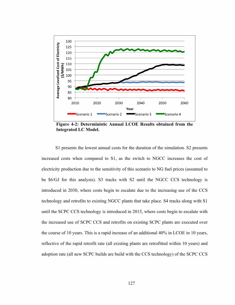
127

Figure 4-2: Deterministic Annual LCOE Results obtained from the Integrated LC Model.

S1 presents the lowest annual costs for the duration of the simulation. S2 presents

increased costs when compared to S1, as the switch to NGCC increases the cost of

electricity production due to the sensitivity of this scenario to NG fuel prices (assumed to

be $6/GJ for this analysis). S3 tracks with S2 until the NGCC CCS technology is

introduced in 2030, where costs begin to escalate due to the increasing use of the CCS

technology and retrofits to existing NGCC plants that take place. S4 tracks along with S1

until the SCPC CCS technology is introduced in 2015, where costs begin to escalate with

the increased use of SCPC CCS and retrofits on existing SCPC plants are executed over

the course of 10 years. This is a rapid increase of an additional 40% in LCOE in 10 years,

reflective of the rapid retrofit rate (all existing plants are retrofitted within 10 years) and

adoption rate (all new SCPC builds are build with the CCS technology) of the SCPC CCS

128

technology. Costs for scenarios 2 through 4 begin to stabilize after transition periods (i.e.,

technology switching, and CCS technology introduction).

As with the environmental performance results in Figure 4-1, these cost results

are useful in that they can demonstrate the effect of generation technology choices and

introduction on overall costs, but do not include the uncertainty in cost of the technology

use. For example, the costs of the NGCC CCS technology are highly uncertain, and the

price of NG is represented with a single value, where in reality it is prone to fluctuation.

Decisions based on cost are susceptible to the same potentially overly optimistic results

as for the decisions based on environmental performance. For example, S3 could

potentially become more costly than S4 if the NGCC CCS costs used in the analysis are

lower than actual costs, and NG prices are higher on average than $6/GJ. The following

sections of this chapter present methods to address uncertainty, and provide a means to

go beyond deterministic analyses of advanced CCS technology.

2.2 Deterministic Sensitivity Analysis

This section presents results from deterministic sensitivity methods used to

explore the effect of variation in parameter values on the overall results, with the goal of

informing subsequent analyses on influential factors (those with the largest impacts on

the results) and thus provide a focal point for uncertainty analysis. Case study

deterministic sensitivity results for the individual scenarios are split into two main

categories, 1) the environmental performance in terms of cumulative life cycle GHG

emissions and 2) the cumulative life cycle cost of electricity, both over the period of 100

years.

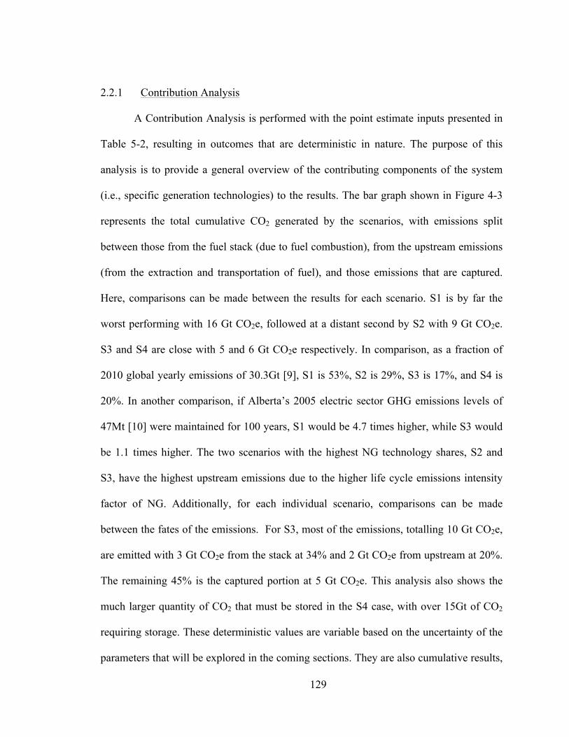
129

2.2.1 Contribution Analysis

A Contribution Analysis is performed with the point estimate inputs presented in

Table 5-2, resulting in outcomes that are deterministic in nature. The purpose of this

analysis is to provide a general overview of the contributing components of the system

(i.e., specific generation technologies) to the results. The bar graph shown in Figure 4-3

represents the total cumulative CO2 generated by the scenarios, with emissions split

between those from the fuel stack (due to fuel combustion), from the upstream emissions

(from the extraction and transportation of fuel), and those emissions that are captured.

Here, comparisons can be made between the results for each scenario. S1 is by far the

worst performing with 16 Gt CO2e, followed at a distant second by S2 with 9 Gt CO2e.

S3 and S4 are close with 5 and 6 Gt CO2e respectively. In comparison, as a fraction of

2010 global yearly emissions of 30.3Gt [9], S1 is 53%, S2 is 29%, S3 is 17%, and S4 is

20%. In another comparison, if Alberta’s 2005 electric sector GHG emissions levels of

47Mt [10] were maintained for 100 years, S1 would be 4.7 times higher, while S3 would

be 1.1 times higher. The two scenarios with the highest NG technology shares, S2 and

S3, have the highest upstream emissions due to the higher life cycle emissions intensity

factor of NG. Additionally, for each individual scenario, comparisons can be made

between the fates of the emissions. For S3, most of the emissions, totalling 10 Gt CO2e,

are emitted with 3 Gt CO2e from the stack at 34% and 2 Gt CO2e from upstream at 20%.

The remaining 45% is the captured portion at 5 Gt CO2e. This analysis also shows the

much larger quantity of CO2 that must be stored in the S4 case, with over 15Gt of CO2

requiring storage. These deterministic values are variable based on the uncertainty of the

parameters that will be explored in the coming sections. They are also cumulative results,

130

and so therefore do not reflect the emissions-time history of each scenario, as shown in

Figure 4-1. Given the choice between scenarios, and faced with only these results, a

decision maker might choose S2, since results show a 44% decrease over S1 cumulative

emissions is possible without the use of CCS technology.

  CO2 Captured CO2 Emitted at Stack CO2 Emitted Upstream

Figure 4-3: Contribution Results for Environmental Performance in terms of the Cumulative CO2 Emissions. The relative contribution that uncaptured direct emissions (from the combustion of fuel) and from the upstream emissions (from the extraction and transportation of fuel) is contrasted to the amount of CO2 captured.

Results of the Contribution Analysis for the life cycle cost for all the scenarios are

presented in Figure 4-4. Here, the relative cumulative costs (trillions dollars over 100

years) for various generation technologies can be contrasted and compared to the total

cumulative cost for the 100 years period. The total cost of S1 is 1.89 trillion dollars. The

largest contributor for S1 is SCPC at 44%, followed by cogeneration at 35%, NGSC at

16%, NGCC at 4%, and PC at 1%. The total cost of S2 is 1.93 trillion dollars. The

Scenario 1 Scenario 2

Scenario 3 Scenario 4

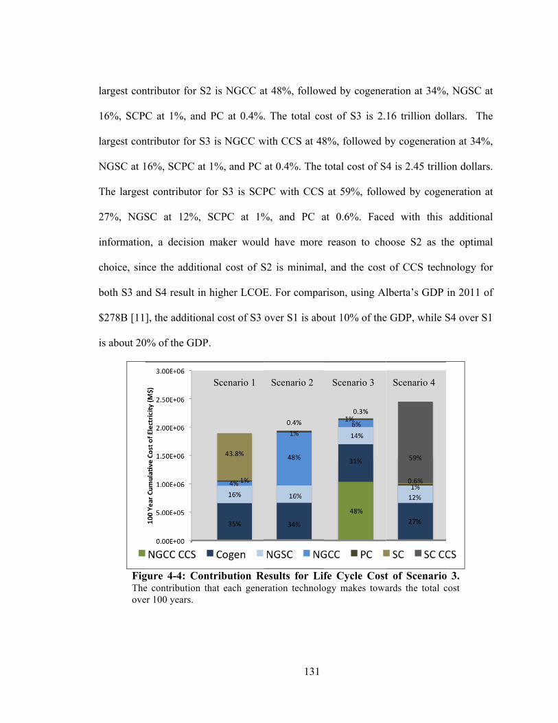
131

largest contributor for S2 is NGCC at 48%, followed by cogeneration at 34%, NGSC at

16%, SCPC at 1%, and PC at 0.4%. The total cost of S3 is 2.16 trillion dollars. The

largest contributor for S3 is NGCC with CCS at 48%, followed by cogeneration at 34%,

NGSC at 16%, SCPC at 1%, and PC at 0.4%. The total cost of S4 is 2.45 trillion dollars.

The largest contributor for S3 is SCPC with CCS at 59%, followed by cogeneration at

27%, NGSC at 12%, SCPC at 1%, and PC at 0.6%. Faced with this additional

information, a decision maker would have more reason to choose S2 as the optimal

choice, since the additional cost of S2 is minimal, and the cost of CCS technology for

both S3 and S4 result in higher LCOE. For comparison, using Alberta’s GDP in 2011 of

$278B [11], the additional cost of S3 over S1 is about 10% of the GDP, while S4 over S1

is about 20% of the GDP.

Figure 4-4: Contribution Results for Life Cycle Cost of Scenario 3. The contribution that each generation technology makes towards the total cost over 100 years.

Scenario 1 Scenario 2 Scenario 3 Scenario 4

132

The results of the Contribution Analysis can be used for gaining an understanding

of the breakdown of contributions in the system, to determine important aspects of the

technologies in use, and for use in determining further data gathering or representation

needs. For example, in Scenario 3, the relative contribution of upstream emissions is

significant at 20% of the total emissions released to the atmosphere. In terms of

technology evaluation, this means that the consideration of impacts related to the

upstream extraction and transport of fuel is an important aspect that should not be

ignored. Similarly, over 90% of the costs in Scenario 3 are the result of using NG

technologies. Therefore, the price of NG (assumed to be $6/GJ in the base case) will

therefore have a large impact on the results between different scenarios, meaning that

further sensitivity analysis would be beneficial given that future natural gas prices are

highly uncertain.

2.2.2 Perturbation Analysis

This section presents results of a method used to determine which parameters

have the largest influence on results through a small variation in value (a perturbation).

The Perturbation Analysis does not use predetermined ranges for the analysis, but rather

uses a relatively small (±5%) and consistent (across all parameters) perturbation for one

parameter at a time to generate a small change in result value. The analysis uses the

calculation of Sensitivity Ratios (SR) to determine the ranking and magnitude of the

influence; higher SR values indicate the most influential of these parameters, or those that

affect the results the most through a small variation in value. For magnitude, a SR of 1

indicates that a 5% change in the parameter value results in a 5% change in the outcome,

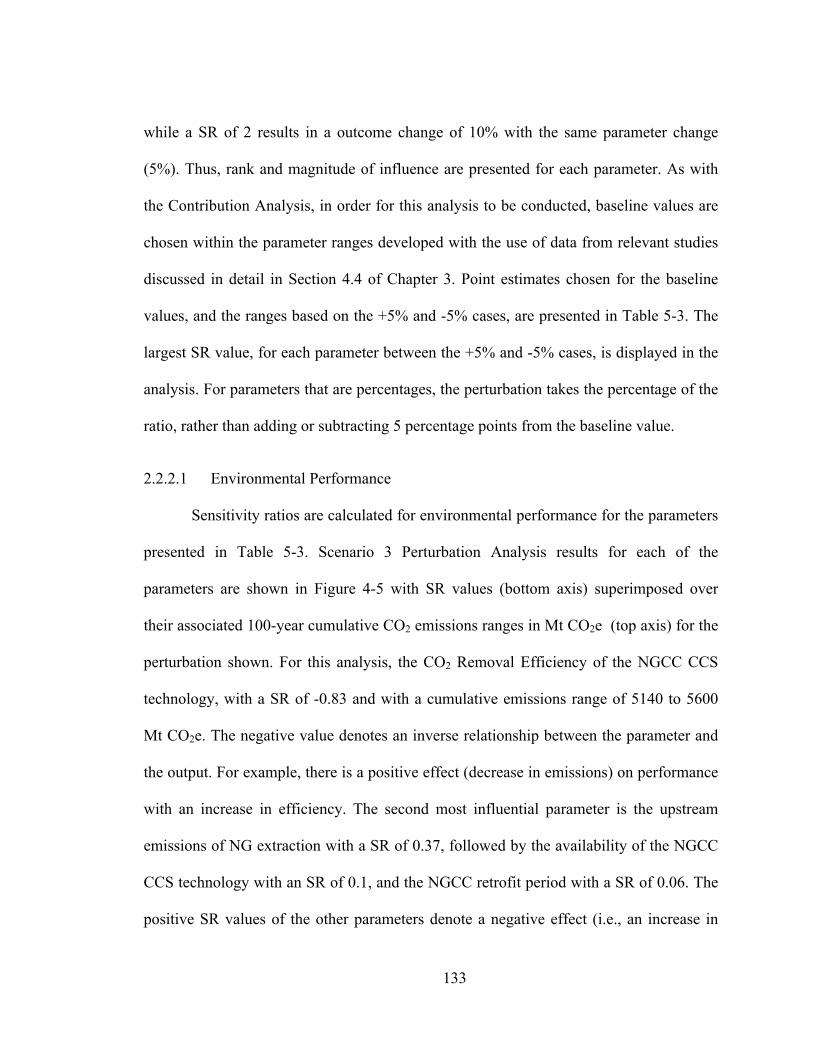
133

while a SR of 2 results in a outcome change of 10% with the same parameter change

(5%). Thus, rank and magnitude of influence are presented for each parameter. As with

the Contribution Analysis, in order for this analysis to be conducted, baseline values are

chosen within the parameter ranges developed with the use of data from relevant studies

discussed in detail in Section 4.4 of Chapter 3. Point estimates chosen for the baseline

values, and the ranges based on the +5% and -5% cases, are presented in Table 5-3. The

largest SR value, for each parameter between the +5% and -5% cases, is displayed in the

analysis. For parameters that are percentages, the perturbation takes the percentage of the

ratio, rather than adding or subtracting 5 percentage points from the baseline value.

2.2.2.1 Environmental Performance

Sensitivity ratios are calculated for environmental performance for the parameters

presented in Table 5-3. Scenario 3 Perturbation Analysis results for each of the

parameters are shown in Figure 4-5 with SR values (bottom axis) superimposed over

their associated 100-year cumulative CO2 emissions ranges in Mt CO2e (top axis) for the

perturbation shown. For this analysis, the CO2 Removal Efficiency of the NGCC CCS

technology, with a SR of -0.83 and with a cumulative emissions range of 5140 to 5600

Mt CO2e. The negative value denotes an inverse relationship between the parameter and

the output. For example, there is a positive effect (decrease in emissions) on performance

with an increase in efficiency. The second most influential parameter is the upstream

emissions of NG extraction with a SR of 0.37, followed by the availability of the NGCC

CCS technology with an SR of 0.1, and the NGCC retrofit period with a SR of 0.06. The

positive SR values of the other parameters denote a negative effect (i.e., an increase in

134

emissions) with an increase in parameter value. The SR value of the availability of the

NGCC CCS technology is smaller using the +5% case (SR = 0.06) with a change in total

emissions of +15.3 Mt CO2e, versus -27.6 Mt CO2e for the -5% case (SR = 0.1),

reflecting that it has more influence with earlier availability times. This implies that

earlier introduction times for the NGCC CCS technology have greater effect on the

environmental performance of the scenario.

Figure 4-5: Perturbation Analysis for Environmental Performance of Scenario 3 – NGCC with CCS. SR values are shown with green bars (bottom axis) superimposed over the associated cumulative CO2 emissions ranges shown with blue bars (top axis). Negative SR values denote that an increase in the parameter value results in a decrease in result, and positive SR values denote an increase in result.

The decision between scenarios may ultimately come down to S3 and S4, since

both offer the greatest reduction in emissions. Some parameters will have similar

influence on both scenarios, while others will only influence one scenario. Sensitivity

ratios are calculated for the difference in environmental performance results between S3

and S4 (Scenario 3 minus Scenario 4), shown in Figure 4-6. The purpose of this exercise

is to explore the sensitivity of the difference between S3 and S4 (i.e., the scenarios with

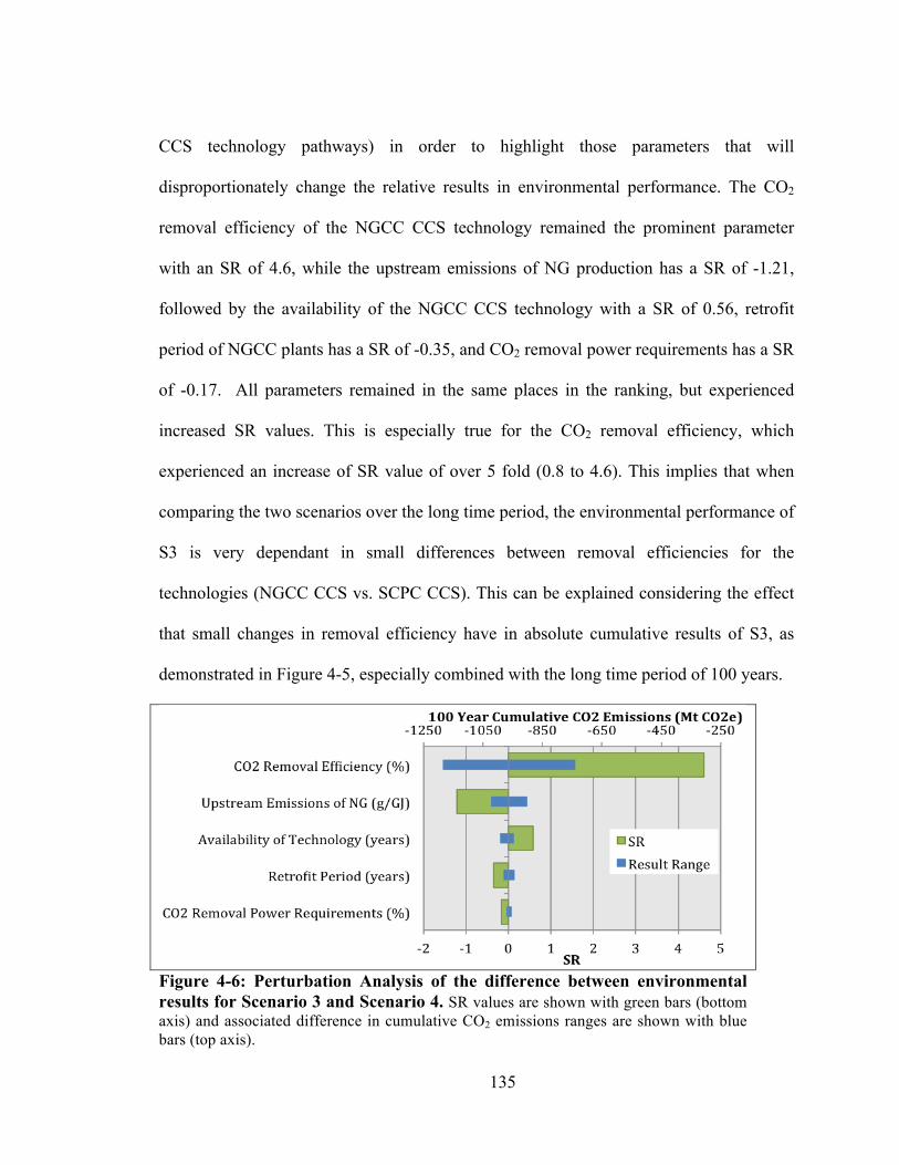
135

CCS technology pathways) in order to highlight those parameters that will

disproportionately change the relative results in environmental performance. The CO2

removal efficiency of the NGCC CCS technology remained the prominent parameter

with an SR of 4.6, while the upstream emissions of NG production has a SR of -1.21,

followed by the availability of the NGCC CCS technology with a SR of 0.56, retrofit

period of NGCC plants has a SR of -0.35, and CO2 removal power requirements has a SR

of -0.17. All parameters remained in the same places in the ranking, but experienced

increased SR values. This is especially true for the CO2 removal efficiency, which

experienced an increase of SR value of over 5 fold (0.8 to 4.6). This implies that when

comparing the two scenarios over the long time period, the environmental performance of

S3 is very dependant in small differences between removal efficiencies for the

technologies (NGCC CCS vs. SCPC CCS). This can be explained considering the effect

that small changes in removal efficiency have in absolute cumulative results of S3, as

demonstrated in Figure 4-5, especially combined with the long time period of 100 years.

Figure 4-6: Perturbation Analysis of the difference between environmental results for Scenario 3 and Scenario 4. SR values are shown with green bars (bottom axis) and associated difference in cumulative CO2 emissions ranges are shown with blue bars (top axis).

136

The CO2 removal efficiency of the NGCC CCS technology is the most influential

parameter, and therefore the results, in both absolute and relative terms, are sensitive to

its variation. Based on the SR value of CO2 removal efficiency of 4.6 for the relative

results of Scenarios 3 and 4, a 1% change in the parameter value will result in a change of

4.6% in the difference between scenario results. For stakeholders assessing choices

between NG and coal CCS technologies, this means that consideration should be given to

the higher uncertainty of the NGCC CCS technology performance compared to SCPC

CCS. The analysis indicates that removal efficiency deficiencies for NGCC CCS on the

order of a few percentage points results in much larger effects on the relative

performance against the coal technology. Consequently, the future performance of the

NGCC CCS technology, in terms of CO2 capture efficiency, should be a large factor

when comparing technologies. Additionally, based on this analysis and the previous

Contribution Analysis, the upstream emissions factor highly in the overall environmental

performance assessment of the scenarios. This is a concern since uncertainty exists

surrounding the actual emissions resulting from current unconventional NG extraction

(i.e., expressed with a range between 6.6 and 15 kgCO2e/GJ of NG extracted), but also

exists in future extraction as reservoirs are more fully exploited, resulting in greater

uncertainty in fugitive emissions [12]. Finally, the retrofit period is more influential to

both relative and absolute performance than the technology availability when looking at

later NGCC CCS technology introduction times. While the availability time of the

technology (when the technology is deployed) is close in magnitude of influence, the rate

137

of technology adoption in existing plants (rate of retrofits to NGCC plants) is an

important aspect of the system’s environmental performance.

2.2.2.2 Life Cycle Cost

The LC cost of the scenarios is expressed as the 100 year average Levelized Cost

of Electricity (LCOE) in $/MWh, which is the average cost to produce electricity across

the system over the time period of 100 years. SR values of the life cycle cost of S3 are

depicted in Figure 4-7. Of those parameters, NG Price has the highest SR at 0.50. The

second most influential parameter is the CRF with a SR of 0.29, followed by the capacity

factor of NGCC plants with a SR of -0.21. The remaining parameters have SR values

below 0.1, meaning that they are less than half as influential than the third highest ranked

parameter, the capacity factor. The top two parameters are those that apply to the whole

system, thus their variation affects the cost across the system. Within the parameters that

are specific to the NGCC plants with CCS technology, the capital required for the CCS

technology is the most influential with an SR of 0.06, followed by the variable O&M

with an SR of 0.03, the retrofit penalty with an SR of 0.03, and the CO2 removal

efficiency with an SR of -0.02.

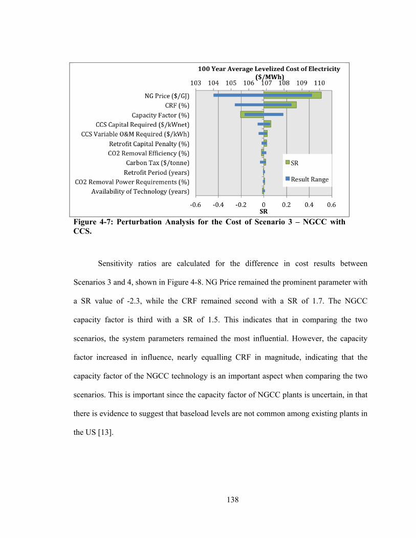
138

Figure 4-7: Perturbation Analysis for the Cost of Scenario 3 – NGCC with CCS.

Sensitivity ratios are calculated for the difference in cost results between

Scenarios 3 and 4, shown in Figure 4-8. NG Price remained the prominent parameter with

a SR value of -2.3, while the CRF remained second with a SR of 1.7. The NGCC

capacity factor is third with a SR of 1.5. This indicates that in comparing the two

scenarios, the system parameters remained the most influential. However, the capacity

factor increased in influence, nearly equalling CRF in magnitude, indicating that the

capacity factor of the NGCC technology is an important aspect when comparing the two

scenarios. This is important since the capacity factor of NGCC plants is uncertain, in that

there is evidence to suggest that baseload levels are not common among existing plants in

the US [13].

139

Figure 4-8: Perturbation Analysis of the Difference Between Cost Results for Scenario 3 and Scenario 4.

NG Price stands out as the most influential parameter in both relative and absolute

cost results for S3. This is expected since the scenario has a large share of NG

technologies as shown in the previous Contribution Analysis (see Figure 4-4). The

importance of NG price on the relative rankings of the scenarios lends itself to further

investigation, with a Scenario Analysis used in the Stochastic Sensitivity Analysis in

Section 2.4.1, and another method using a Combined Sensitivity Analysis performed later

on in Section 2.4.5. The Capital Recovery Factor (CRF) is a close second in influence.

This is a potentially important aspect of the results since CRF for riskier technologies are

potentially higher than for other more established technologies [13]. While this thesis

assumes a common CRF across all technologies, further work investigating the impact of

risk factors in capital cost may be of interest.

140

2.3 Uncertainty Analysis

Following the Deterministic Sensitivity Analysis completed above, an

Uncertainty Analysis is performed to quantify the uncertainty in the results. While the

sensitivity analysis provides information about the sensitivity of the results to variation, it

does not quantify the uncertainty. A similar analysis passing the maximum and minimum

value of all the parameters through the model can provide the extremes of the results, can

improve on the Perturbation Analysis by providing a range of performance and cost

results. However, it does not provide the probability of these events happening. An

Uncertainty Propagation Analysis uses probability distributions and a sampling method to

create probability distributions for the results. The key parameters discussed in Chapter 3

are represented using the baseline set of probability distributions described in Table 5-4,

which are then randomly sampled from a Monte Carlo Simulation (MCS). The MCS

provides the samples as inputs to the Integrated LC Model. In all cases, the MCS is run

for 10,000 iterations. This provides cost and environmental performance outcomes for

each scenario expressed as probability distributions, which can be compared and ranked

using a Discernibility Analysis. The initial choices for probability distributions are

presented as a ‘baseline’ set in Table 5-4 and Table 5-5, with the effects of additional

distribution choices explored in a Stochastic Sensitivity Analysis in Section 2.4.2.

Since a carbon tax would be introduced to help more costly low carbon

technologies become more competitive (i.e., by increasing costs for more carbon

intensive technologies), a value of zero is used for the initial uncertainty analysis to

observe the results without the influence of a carbon tax on the system. Further analysis

141

on the effect of a carbon tax is completed in Section 2.4.5 as part of the Combined

Sensitivity and Uncertainty Propagation Analysis.

2.3.1 Uncertainty Propagation Analysis

Using the baseline probability distributions, as presented in Table 5-4 and Table

5-5, a MCS is performed for Scenarios 1 through 4 with 10,000 iterations. Each MCS

iteration is executed in parallel across the scenarios (i.e., sampled system parameters

values, such as NG price, are equal for all scenarios for each iteration) rather than

independently applied (i.e., sampled system parameters values are not equal for all

scenarios for each iteration). This provides result distributions containing 10,000

samples, that for any given MCS iteration, the results for each scenario are comparable

since they would experience similar NG price values. Three different results are provided

for each scenario; environmental performance, life cycle cost, and abatement cost.

Environmental performance results of the scenarios are similar to the above analysis, but

are expressed as a probability distribution of the cumulative LC GHG emissions over 100

years in Mt CO2e. The LC cost of the scenarios is expressed as a distribution for the 100

year average Levelized Cost of Electricity (LCOE) in $/MWh. Finally, the CO2

Abatement Cost results are presented for Scenario 3. The abatement cost results for S3

are presented for two different reference scenarios, S1 and S2, since both could be

considered baseline. In a possible future scenario where Alberta has made the switch to

NG from coal, S2 is a more appropriate baseline, as so is included in the calculation of

abatement costs.

2.3.1.1 Environmental Performance

142

Environmental performance results from the Uncertainty Propagation Analysis

using MCS are presented in Figure 4-9 as a histogram, with the cumulative GHG

emissions as the x-axis (Mt CO2e) and the relative population density of the distribution

as the y-axis (%). S1 is the worst performing with a mean of 160 Gt of CO2e over 100

years. S2 is second worst at a mean of 92 Gt of CO2e over 100 years. S3 and S4 overlap

with means of 57 and 63 Gt of CO2e respectively. S1 and S2 have clearly defined zones

within the spectrum of emissions results. Results from this analysis clearly show the

wider range of values possible with a scenario using CCS technology that is less mature,

as in S3. Here, Scenario 3 spans a much wider range, extending past the possible values

for S4, which has a much higher relative population density.

Figure 4-9: Uncertainty Propagation Analysis for Environmental Performance as the 100-year Cumulative LC Emissions. The analysis is completed using a Monte Carlo Simulation with 10000 runs.

This has bearing on the ability of S3 to meet the GHG emissions reduction goals

described in Chapter 1 and summarised in Table 1-1. In addition to cumulative emissions,

143

the Framework also provides performance results for individual years, in terms of yearly

GHG emissions. Using the onsite total plant emissions results for the year 2050 (not

including upstream emissions), and considering the Alberta 2050 goal of 40 Mt

(reduction of 14% based on 2005 emissions) a probability of achieving the goal can be

calculated for each scenario. In this analysis, the assumption is made that Alberta’s

electric sector will maintain a 20% share of the total GHG emissions in the province.

Both S1 and S2 have 0% likelihood, S3 has 30% likelihood, while S4 has 100%

likelihood of achieving the target. In S4, the SCPC CCS technology is implemented

earlier than the NGCC CCS technology, while for S3, uncertainty in the timing of

introduction and performance of the NGCC CCS technology results in less certainty of

success when considering future goals.

2.3.1.2 Life Cycle Cost

Cost results from the Uncertainty Propagation Analysis using MCS are presented

in Figure 4-10 for the stable NG Price case with the 100-year average LCOE ($/MWh) as

the x-axis (Mt CO2e) and the relative population density of the distribution as the y-axis

(%). There is some level of overlap between the scenarios in this case. Scenarios 1 and 2

are the lowest in terms of cost and are close with a mean of $86/MWh and $93/MWh

respectively.

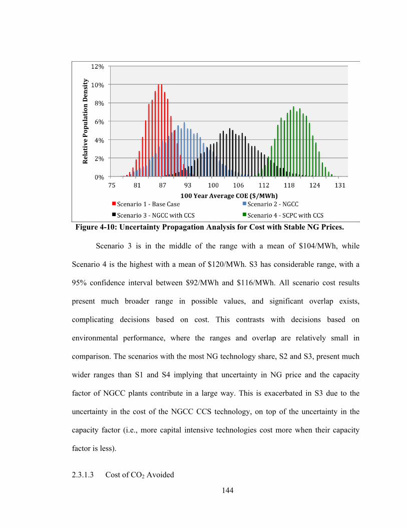
144

Figure 4-10: Uncertainty Propagation Analysis for Cost with Stable NG Prices.

Scenario 3 is in the middle of the range with a mean of $104/MWh, while

Scenario 4 is the highest with a mean of $120/MWh. S3 has considerable range, with a

95% confidence interval between $92/MWh and $116/MWh. All scenario cost results

present much broader range in possible values, and significant overlap exists,

complicating decisions based on cost. This contrasts with decisions based on

environmental performance, where the ranges and overlap are relatively small in

comparison. The scenarios with the most NG technology share, S2 and S3, present much

wider ranges than S1 and S4 implying that uncertainty in NG price and the capacity

factor of NGCC plants contribute in a large way. This is exacerbated in S3 due to the

uncertainty in the cost of the NGCC CCS technology, on top of the uncertainty in the

capacity factor (i.e., more capital intensive technologies cost more when their capacity

factor is less).

2.3.1.3 Cost of CO2 Avoided

145

In this analysis, values for both cost and emissions for Scenario 3 are used from

the Uncertainty Propagation Analysis resulting in a distribution for CO2 abatement costs.

Abatement costs are calculated by dividing the total costs to reduce emissions (difference

in total costs between the lower carbon scenario and a reference scenario) by the

reduction in emissions achieved (difference in emissions between the lower carbon

scenario and a reference scenario). The abatement cost results for S3 are calculated using

both S1 and S2 as reference cases, presented in Figure 4-11 with the 100 year abatement

cost as the x-axis ($/t CO2e abated) and the relative population density of the distribution

as the y-axis (%). The S2 reference case result has a higher average at $68/t CO2, and

wider distribution for the cost of CO2 avoided when compared to the S1 reference case

result, with an average of $34/t CO2.

Figure 4-11: Uncertainty Propagation Analysis for Cost of CO2 Abatement for Scenario 3. CO2 abatement cost results are presented for stable NG Prices.

The lower values from the S1 reference case are due to the much higher CO2

emissions from S1, which presents a larger denominator in the CO2 Abatement Cost

equation. S2 presents a lower range of CO2 emissions, resulting in a smaller denominator

146

and subsequently higher CO2 abatement costs. The values here are lower than what is

presented in existing literature [1-8], since the NGCC CCS technology explored here is

advanced with highly uncertain costs. The ranges used in this analysis represents a

reduction in input costs (capital and variable O&M) up to 25% from values used in

existing studies [1-8], and therefore must be less costly. The results presented here

demonstrate a method of informing stakeholders about the range of prices of carbon

required for NGCC CCS incentivization, and show how aggressively the costs need to be

reduced in order for S3 to be competitive. These results suggest carbon prices that are

higher than any currently being discussed.

2.3.2 Discernibility Analysis

Results from the Discernibility Analysis are summarized in Table 4-1. This

analysis resolves the differences between scenario result distributions obtained from the

Uncertainty Propagation Analysis displayed in Figure 4-9 to Figure 4-10. Columns in the

table represent the scenario of interest, while the rows represent the competing scenario.

For example, there is an 84% probability that Scenario 3 (Row 3) has better

environmental performance (lower emissions) than Scenario 4 (Column 4). Similarly, for

life cycle cost with stable NG prices, Scenario 3 has a 100% probability of having lower

cost than Scenario 4.

Table 4-1: Discernibility Analysis Results for both Environmental Performance and Life Cycle Cost for all Scenarios.

  Environmental  Performance   Cost  with  Stable  NG  Prices  

Scen.   1   2   3   4   1   2   3   4  1   -­‐   0%   0%   0%   -­‐   96%   100%   100%  2   100%   -­‐   0%   0%   4%   -­‐   100%   100%  3   100%   100%   -­‐   84%   0%   0%   -­‐   100%  4   100%   100%   16%   -­‐   0%   0%   0%   -­‐  

147

2.4 Stochastic Sensitivity Analysis

Data regarding the NGCC CCS technology parameters are sparse and the method

used to develop the probability distributions does not characterize them precisely (e.g.,

through shape, mean, and skewness). A Stochastic Sensitivity Analysis is performed to

assess the effects of variation in the input parameter distribution characteristics used in

the Uncertainty Analysis performed in the previous section. Five separate analyses are

used; a Probability Distribution Scenario Analysis, a Probability Distribution Type

Sensitivity Analysis, a Relative Degree of Optimism Analysis, a Technology Availability

and Improvement Analysis, and a Combined Sensitivity and Uncertainty Propagation

Analysis.

2.4.1 Probability Distribution Scenario Analysis

A Probability Distribution Scenario Analysis uses the constructs of scenarios to

frame the uncertainty in parameters of interest. This analysis adds to the set of scenarios

used in the analysis (the generation technology scenarios 1 to 4) and is used here to assess

the effects of different NG Price parameter distributions on the overall results.

Considering the large impact that NG Price has on the cost results, two scenarios (for

clarity hereon referred to as cases) for the degree of NG Price stability (i.e., stable and

unstable cases) are used to expand on the range of cost results, represented in Figure 4-12.

The initial Uncertainty Analysis results conducted above uses the stable case to represent

current long-term forecasts [14], while results for the unstable case are presented below.

Both cases use beta probability distributions using the range of $3 - $10/GJ and have a

mean of $6/GJ, while the standard deviations are $0.90/GJ and $1.46/GJ for the stable

148

and unstable cases respectively. In the unstable case, the distribution is designed to skew

toward the lower end (as shown graphically in Figure 4-12), representing the tendency of

the price to be in the lower range.

Figure 4-12: Chosen Probability Distributions for NG Price. Two scenarios are represented, a scenario where NG Price is relatively stable, and one where the price is unstable. Both have a mean of $6/GJ to account for the price of NG over the period of 100 years.

The two scenarios with the highest NG technology share (S2 and S3) experience

the most variation in cost results, which is exacerbated in the unstable NG price case, as

shown in Figure 4-13, which uses the same inputs used in the analysis presented in Figure

4-10, except for the addition of unstable NG price. In the unstable NG Price case, the

range of cost results for S3 extend well into the range of S4 results, suggesting that the

risk of unstable NG Prices can affect the economic attractiveness of S3 when compared

to the relative stability of S4 costs. This is also demonstrated in the Discernibility Results

presented in Table 4-2, where the probability of S3 costing less than S4 drops from 100%

to 95%. This represents an insignificant difference, meaning that S3 is still significantly

better than S4 in terms of cost. This implies that the volatility of NG prices has little

149

effect on the qualitative conclusions regarding comparisons between S3 and S4.

However, the ranges and uncertainty in NG price still play a large role in the overall cost

results of S3.

Figure 4-13: Uncertainty Propagation Analysis for Cost for Unstable NG Prices.

Table 4-2: Discernibility Analysis Results for Life Cycle Cost for Stable and Unstable NG Prices.

  Cost  Stable  NG  Prices   Unstable  NG  Prices  

Scen.   1   2   3   4   1   2   3   4  1   -­‐   96%   100%   100%   -­‐   78%   100%   100%  2   4%   -­‐   100%   100%   22%   -­‐   100%   100%  3   0%   0%   -­‐   100%   0%   0%   -­‐   95%  4   0%   0%   0%   -­‐   0%   0%   5%   -­‐  

The abatement cost is generally considered a guide for the value of a carbon tax

that is required to make a GHG mitigation technology economically attractive [8]. In the

case of the NGCC with advanced CCS technology under investigation here, the tax value

required would be higher in the reference scenario where NG technologies are dominant,

150

such as in S2. While on the other hand, the tax would be less using the reference scenario

where coal is dominant, such as in S1. The distributions presented in Figure 4-14, using

cumulative distributions (rather than histograms) obtained from Uncertainty Analysis,

present the results of abatement costs in a way that allows for better comparison of the

uncertainty in outcomes. Results are presented for the stable NG price case for the S1 and

S2 references, and for the unstable NG price case for S1. The x-axis is the 100-year

abatement costs ($/t CO2e abated) and the y-axis is the cumulative relative population

density.

Figure 4-14: Uncertainty Propagation Analysis for Cost of CO2 Abatement for Scenario 3. A 95% confidence level is marked, with intercepts drawn for each case.

Statistically significant values are obtained by determining the value at which the

cumulative curve of the result reaches 95% (indicated by arrows). For example, as

demonstrated in Figure 4-14, the carbon tax required with S1 as reference case and with

stable NG prices is $48/t CO2e. In the case of unstable NG prices for the S1 reference, a

higher value at $60/t CO2e is required. In addition, this analysis indicates that for the S2

151

reference case, abatement costs need to be higher than the mean value ($68/t CO2e)

expressed in Figure 4-11. Using the 95% confidence level, carbon taxes for the S2

reference case require $86/t CO2e. The instability of NG prices is cancelled out for the S2

reference case, since both S2 and S3 have the same NG technology share. Results in

Figure 4-14 suggest that carbon taxes are not well represented as deterministic values. In

other words, the tax required to make the technology break even economically will be

different depending on the economic conditions in the system. Given that NG prices are

prone to fluctuation, this implies that those setting carbon tax policies would need to

consider fluctuation accordingly to properly incentivise NGCC CCS technologies when

there is coal in the system.

2.4.2 Probability Distribution Type Sensitivity Analysis

As mentioned above, data regarding the NGCC CCS technology parameters are

sparse. The method used in this analysis to develop the probabilities distributions,

through the use of ranges derived from literature and choice of shape through judgement

based on the nature of the parameter and quality of data, does not characterize the shape

in a precise manner. The robustness of the results obtained from the Uncertainty Analysis

is dependent on the robustness of the inputs used. Therefore there is a need to understand

the impact of the assumptions used in developing the distributions on the results. A

Probability Distribution Type Sensitivity Analysis is used to assess the impacts of

imprecise parameter distribution shapes used for uncertainty propagation analysis. In this

analysis, three separate MCS runs are conducted where the technology input parameter

distributions are represented first with all uniform, then followed with all triangular, and

152

all beta distribution types. These results are then compared to the baseline distribution set

used in the previous analyses described in Table 5-4. The results of the Probability Type

Sensitivity Analysis for Scenario 3 Abatement Costs are presented in Figure 4-15. Here,

four separate abatement cost histogram results, one for each type of probability

distribution, are presented.

Figure 4-15: Effect of Probability Distribution Type on the Abatement Cost of Scenario 3 using Scenario 2 as a Reference. Results in terms of abatement cost displayed as relative population density are shown for the baseline, uniform, triangular, and beta distributions used for the technology parameters.

Results of this analysis show that the effect of choice of distribution type has little

effect on the overall abatement cost results for Scenario 3. This is most clearly seen when

presented with a cumulative population curve as shown in Figure 4-16. This does not

necessarily imply complete knowledge, or robust distribution representation. In situations

where other parameters have greater influence on the results (i.e., NG price, CRF) the

effect of distribution shape is less important. Of the distribution shapes, the most

noticeable change in abatement cost results comes from the uniform distribution case.

153

This implies that in situations where the distributions are inappropriately represented as

uniform (as with many parameters with sparse data [15]), the robustness of the overall

results will be affected to some degree. The degree will depend on the relative magnitude

of the influence of the parameter on the results, such that higher magnitudes of influence

will exacerbate the effect of distribution shape misrepresentation. The mitigation strategy

here for an analyst would be to avoid using uniform distributions for influential

parameters, and focus research to gather additional data, or use a proxy technology to

supplement the data.

Figure 4-16: Effect of Probability Distribution Type on the Abatement Cost of Scenario 3 using Scenario 2 as a Reference. Results in terms of abatement cost displayed as cumulative population density are shown for the baseline, uniform, triangular, and beta distributions used for the technology parameters.

2.4.3 Relative Degree of Optimism Analysis

Data are sparse regarding the extremal bias in technology parameter distributions

described in Chapter Three: 4.4. Since the NGCC CCS technology is highly uncertain in

that it represents a technology that is improved up to 25% in performance and cost, there

is a possibility that the baseline distributions are overly optimistic in their representation.

For example, the capital cost of the NGCC CCS technology (represented with a uniform

154

distribution in the baseline set in Table 5-5) may be overly optimistic in representing

equal probability for costs in the range. In reality, a bias may exist towards either end of

the range. A Relative Degree of Optimism (RDO) Analysis is used to account for the

possibility that the baseline probability distributions used in the Uncertainty Propagation

Analysis are not correctly representing the skewness, or extremal tendency of the inputs

within the specified ranges for the technology parameters (see Table 5-4).

The system parameters retain their baseline distributions so that the analysis can

focus on the effects of the uncertainty in the technology input distributions on the overall

results. Based on the results of the previous Distribution Type Sensitivity Analysis, the

results differ very little when beta distributions are substituted for the baseline

distributions. Therefore, beta distributions can be used in place of the baseline

distributions to represent the parameters, allowing for beta shape parameters to be

systematically changed to explore the skewness and extrema within the ranges and

account for pessimistic (high costs, poor performance) or optimistic (low cost, good

performance) representation.

Environmental performance results from the RDO Analysis for S3 are presented

in Figure 4-17. Here, four results for the 100-year cumulative CO2 emissions are

presented; two for a pessimistic and optimistic case for S3, the baseline case for S3, and

the results for S4. The results for S4 are included in this analysis to provide a comparison

to an alternative GHG mitigation scenario with a less uncertain technology. In the

pessimistic case, where the technology input distributions are skewed to the least

optimistic extreme (i.e., tendency to higher cost, higher parasitic power, lower CO2

capture rate), the results experienced an increase of 16% in mean value over the baseline

155

results. In the optimistic case (i.e., tendency to lower cost, lower parasitic power, and

higher capture rate) the cumulative emissions mean value decreased by 11% over the

baseline results. This implies, that with in the confines of the ranges used in the analysis,

the technology can have very different performance results, confusing the analysis when

considering emissions and relative performance to the alternative scenario (S4).

Figure 4-17: Relative Degree of Optimism Analysis Results for Scenario 3 Cost and Environmental Performance. Effect of RDO in technology parameter values on S3 cumulative emissions over 100 years.

This can also be analysed further using a Discernibility Analysis, presented in

Table 4-3. The effect of higher optimism results in an increased level of confidence in

having lower emissions than S4 by 16% (84% compared to 100%). The effect of

pessimistic inputs results in a decrease in confidence level by 36% (84% compared to

48%). This implies reinforces that previous implication that, within the ranges developed

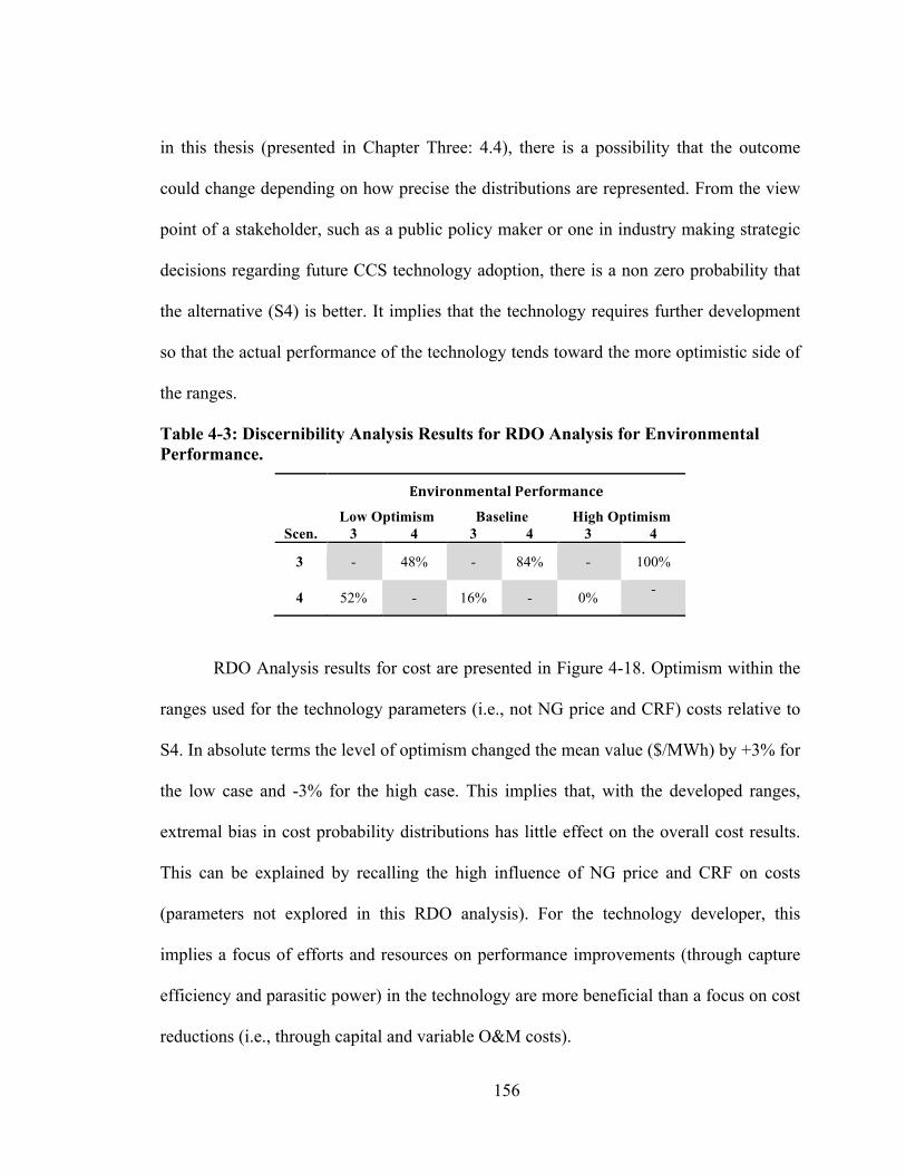
156

in this thesis (presented in Chapter Three: 4.4), there is a possibility that the outcome

could change depending on how precise the distributions are represented. From the view

point of a stakeholder, such as a public policy maker or one in industry making strategic

decisions regarding future CCS technology adoption, there is a non zero probability that

the alternative (S4) is better. It implies that the technology requires further development

so that the actual performance of the technology tends toward the more optimistic side of

the ranges.

Table 4-3: Discernibility Analysis Results for RDO Analysis for Environmental Performance.

Environmental  Performance  

Scen. Low Optimism Baseline High Optimism

3 4 3 4 3 4

3 - 48% - 84% - 100%

4 52% - 16% - 0% -

RDO Analysis results for cost are presented in Figure 4-18. Optimism within the

ranges used for the technology parameters (i.e., not NG price and CRF) costs relative to

S4. In absolute terms the level of optimism changed the mean value ($/MWh) by +3% for

the low case and -3% for the high case. This implies that, with the developed ranges,

extremal bias in cost probability distributions has little effect on the overall cost results.

This can be explained by recalling the high influence of NG price and CRF on costs

(parameters not explored in this RDO analysis). For the technology developer, this

implies a focus of efforts and resources on performance improvements (through capture

efficiency and parasitic power) in the technology are more beneficial than a focus on cost

reductions (i.e., through capital and variable O&M costs).

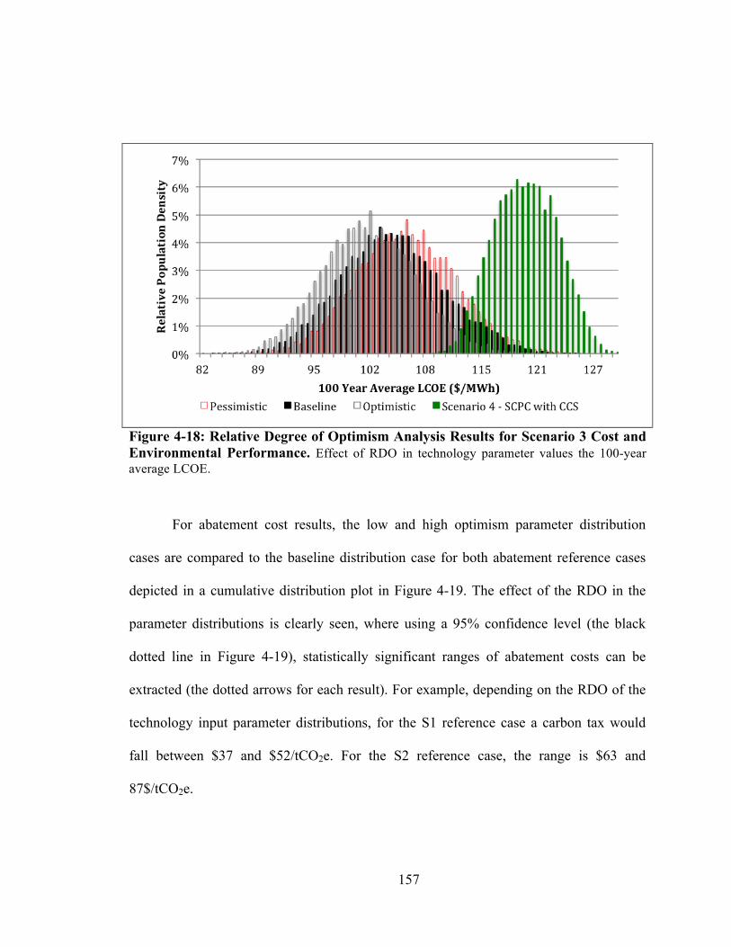
157

Figure 4-18: Relative Degree of Optimism Analysis Results for Scenario 3 Cost and Environmental Performance. Effect of RDO in technology parameter values the 100-year average LCOE.

For abatement cost results, the low and high optimism parameter distribution

cases are compared to the baseline distribution case for both abatement reference cases

depicted in a cumulative distribution plot in Figure 4-19. The effect of the RDO in the

parameter distributions is clearly seen, where using a 95% confidence level (the black

dotted line in Figure 4-19), statistically significant ranges of abatement costs can be

extracted (the dotted arrows for each result). For example, depending on the RDO of the

technology input parameter distributions, for the S1 reference case a carbon tax would

fall between $37 and $52/tCO2e. For the S2 reference case, the range is $63 and

87$/tCO2e.

158

Figure 4-19: Relative Degree of Optimism Results for Scenario 3 Abatement Cost for both Reference Cases using Cumulative Population Density. Results for both reference cases are presented, with a 95% confidence level reflecting statistically significant values for abatement costs.

While the beta parameters are systematically changed in this analysis, the

confidence level of Scenario 3 ranking better than Scenario 4 in terms of environmental

performance and life cycle cost is calculated for a series of RDO points. In doing so, the

relationship between confidence level of ranking higher than S4 (y-axis) and RDO (x-

axis) can be plotted, as demonstrated in Figure 4-20. Here it can be seen that, for

environmental performance, a higher degree of optimism is required to achieve a

confidence level higher than 95% (dotted line). A 10% increase over the mean values

(indicated with an arrow) used in the baseline parameter distributions associated with

environmental performance (e.g., CO2 capture efficiency, parasitic power) is required. In

other words, a breakthrough NGCC CCS technology will require 10% additional

improvement in environmental performance characteristics over what was used in this

thesis (see Table 5-4) in order to be significantly better (95% confidence level) than

SCPC CCS.

159

Figure 4-20: Relative Degree of Optimism Results for Scenario 3 with Confidence Level against Scenario 4. Effect of RDO in technology parameter values on the confidence level of ranking higher (lower cost and lower emissions) than Scenario 4. The effect of relative RDO on confidence level that Scenario 3 would rank higher than Scenario 4 in terms of cost and performance is shown.

2.4.4 Technology Availability and Improvement Analysis

The previous analysis used beta distributions to bias the parameter values from

one extrema to the other without linking the parameters together. For example, cost and

performance are not linked to the time of availability of the technology. However, this is

potentially a false assumption if we suppose that technology cost and performance would

improve overtime, assuming learning curve effects exist [16]. In a Technology

Availability and Improvement Analysis, using the same beta distribution manipulation

method used in the RDO analysis, NGCC CCS technology availability can be linked to

both cost and performance in an inverse relationship, such that the longer the wait for the

technology to be available, the lower the cost and the better the performance of the

technology.

160

Abatement cost results from this analysis for Scenario 3 are displayed in Figure

4-21 using S1 as the reference case, and in Figure 4-22 for the S2 reference case. Here,

the effect of the timing of technology availability combined with technology

improvement can be seen in the abatement costs for S3. Results are presented for an early

case (availability distribution that skews to the lower end of the range), a mid case

(availability distribution that is centred in range), and a late case (availability distribution

that skews to the higher end of the range). An early deployment of a relatively immature

technology (i.e., parameters reflecting less than the 25% improvement in cost and

performance ranges) can be compared to a later deployment of a more mature technology

(i.e., parameters reflecting closer to the full 25% improvement in cost and performance

ranges).

Figure 4-21: Effect of Availability Timing and Improvement in Technology for Scenario 3 Abatement Cost for S1 Reference. Using beta distributions, the improvement in abatement cost over time is simulated by skewing the distributions relative to the year of introduction from early to late availability.

161

Figure 4-22: Effect of Availability Timing and Improvement in Technology for Scenario 3 Abatement Cost for S2 Reference.

The effects seen in this analysis reflect the carbon tax levels needed depending on

the timing of the technology introduction, which also takes into account the improvement

of technology over time. Earlier technology introductions will require higher carbon taxes

to make the technology more attractive, while later introductions will allow for lower

taxes. This is seen clearly in Figure 4-23, where a cumulative population density plot is

presented with a 95% confidence level (dotted line). Here the abatement costs

representing significant ranges based on the early and late technology availability cases

for the S1 reference case is $30 to $64/tCO2e, and for the S2 case is $66 to $95/tCO2e.

For the policy developer, this analysis provides a range of values for carbon price tied to

deployment time estimates for the advanced NGCC CCS technology. This information

could be useful in planning future carbon policies for upcoming GHG mitigation

technology.

162

Figure 4-23: Effect of Availability Timing and Improvement in Technology for Scenario 3 Abatement Costs.

This analysis can also be used to determine an optimal time window (i.e., the

balance between the cost and environmental performance of the scenario) for the

introduction of the NGCC CCS technology in S3 when a 95% confidence level of

outperforming S4 is used. Here, the analysis is conducted for successive technology

availability distributions (by iteratively skewing the distribution from early to late

extremes within the range) while calculating the confidence level of outperforming S4 in

terms of cost and environmental performance. As demonstrated in Figure 4-24, the

relationship between the confidence level of the cumulative cost of S3 being less than for

S4 and the mean of the technology availability (i.e., the mean value of the distribution

used for the technology availability) can be plotted (blue line). Additionally, the

relationship between the confidence level of the cumulative GHG emissions of S3 being

less than for S4 and the mean of the technology availability can also be determined (red

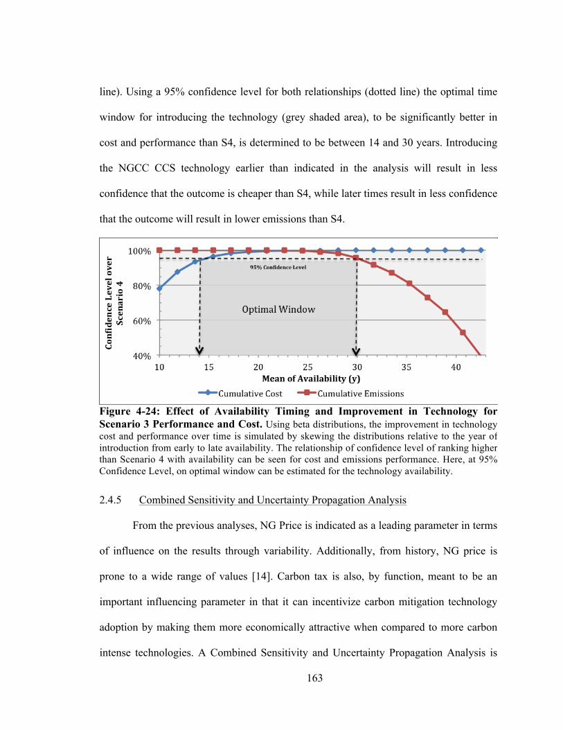
163

line). Using a 95% confidence level for both relationships (dotted line) the optimal time

window for introducing the technology (grey shaded area), to be significantly better in

cost and performance than S4, is determined to be between 14 and 30 years. Introducing

the NGCC CCS technology earlier than indicated in the analysis will result in less

confidence that the outcome is cheaper than S4, while later times result in less confidence

that the outcome will result in lower emissions than S4.

Figure 4-24: Effect of Availability Timing and Improvement in Technology for Scenario 3 Performance and Cost. Using beta distributions, the improvement in technology cost and performance over time is simulated by skewing the distributions relative to the year of introduction from early to late availability. The relationship of confidence level of ranking higher than Scenario 4 with availability can be seen for cost and emissions performance. Here, at 95% Confidence Level, on optimal window can be estimated for the technology availability.

2.4.5 Combined Sensitivity and Uncertainty Propagation Analysis

From the previous analyses, NG Price is indicated as a leading parameter in terms

of influence on the results through variability. Additionally, from history, NG price is

prone to a wide range of values [14]. Carbon tax is also, by function, meant to be an

important influencing parameter in that it can incentivize carbon mitigation technology

adoption by making them more economically attractive when compared to more carbon

intense technologies. A Combined Sensitivity and Uncertainty Propagation Analysis is

164

used to look at the effects of both NG price and carbon tax variation, while accounting

for the uncertainty in other parameters through the use of uncertainty propagation. In

essence it provides the favourable conditions (i.e., price regimes required to rank highest)

for scenarios one through four. Results from this analysis, focusing on S3, are presented

here. In this analysis, several Monte Carlo Simulations are performed for a wide range of

NG price (1 to 20 $/GJ) and carbon tax (0 to 200 $/tonne) values. The analysis ranks

scenario probability distribution results by choosing the one with lowest mean cost for

each NG price and carbon tax point. The highest ranked (lowest cost) scenario is

indicated in a contour plot. Here, favourable NG price (left axis) and carbon tax (top axis)

regimes are depicted in Figure 4-25 through Figure 4-28. This analysis shows the effect

that both carbon tax and NG price have on the ranking of the four scenarios. Lower NG

prices favour S2 and S3, and to some degree S1. The two scenarios with the most carbon

intense technologies (i.e., no CCS), S1 and S2, are only favourable in lower carbon tax

regimes.

165

Figure 4-25: Combined Sensitivity and Uncertainty Propagation Analysis for all Scenarios. The contour plots’ colours represent individual scenarios and the favourable NG price and Carbon Tax conditions for S1 to S4.

Considering that NG technology capacity is increasing in Alberta [17], the

comparison between S2 and S3 (Figure 4-26) is potentially more informative than a

comparison between S1 and S3 (Figure 4-27) since S2 represents the scenario with higher

NG technology share. Here, the higher carbon tax required to incentivise NGCC CCS

technology in with increasingly higher NG price ranges is evident. For example, to

incentivize the NGCC CCS technology, with a NG price of $4/GJ, the carbon tax price

required is $70/t CO2e. The price of carbon would need to increase to $80/t CO2e when

NG prices reach $7/GJ.

S1 – Base Case

S4 - SCPC CCS

S2 - NGCC S3 - NGCC CCS

166

Figure 4-26: Combined Sensitivity and Uncertainty Propagation Analysis for S2 and S3.

A comparison between S1 and S3 (Figure 4-27) shows a more severe relationship

between NG price and carbon tax, where NG price increments of $1/GJ result in

increments of $10/t CO2e for carbon tax. S1 has a lower share of NG technologies, and is

therefore less sensitive to NG price fluctuations. A comparison between S4 and S3

(Figure 4-28) demonstrates that the NG price of over $8/GJ is the threshold where S4 is

less costly than S3. For the policy developer, these results provide information on the

relationship between carbon tax and NG price, and the effects that these costs have on the

overall costs of different generation technology use scenarios.

S2 - NGCC

S3 - NGCC CCS

167

Figure 4-27: Combined Sensitivity and Uncertainty Propagation Analysis for S1 and S3.

Figure 4-28: Combined Sensitivity and Uncertainty Propagation Analysis for S3 and S4.

S1 – Base Case

S3 - NGCC CCS

S4 - SCPC CCS

S3 - NGCC CCS

168

3 Conclusions

3.1 Results Summary

In this chapter, the framework is applied using a case study that assesses various

alternatives to satisfy electricity demand in Alberta over one hundred years, while

incorporating the uncertainty associated with an advanced NGCC CCS technology.

Deterministic results obtained from the Integrated LC Model were presented for both cost

and environmental performance for all scenarios. These results demonstrate the function

of the integrated model by providing a deterministic overview of the performance for

each scenario and the impacts of technology choice on yearly costs and emissions.

Through this analysis the result of not mitigating GHG emissions (S1), or the result of

choosing the least cost path (S2), in electricity production is made clear. It shows the

magnitude of the action required to achieve emissions reductions. Additionally, it shows

that even with CCS, GHG emissions will continue to rise. The implication here is that

RET is an important component of long term GHG emissions reduction policies.

Building on the deterministic results obtained from the Integrated LC Model, the

Uncertainty Assessment Model begins with the use of the Deterministic Sensitivity

Analysis. Using the Contribution Analysis [18] method, this analysis shows the

cumulative emissions and the contributing aspects (i.e., captured, stack, and upstream

emissions) for each scenario. It provides decision-makers with an understanding of the

important aspects of the system. For example, it demonstrates that while S1 had the

highest value, S2 and S3 have higher upstream GHG emissions. This may be a concern

considering the high uncertainty surrounding the upstream emissions associated with

169

unconventional NG extraction. Additionally, through demonstrating the mass of CO2

captured, it shows that S4 must store over threefold the mass of CO2 than S3 must store.

This suggests that consideration of the requirements of additional infrastructure and

storage facilities required for S4 over S3 may be a factor in determining future options

for GHG mitigation. Possible fluctuations in NG price are also a large component in cost

consideration. The Uncertainty Assessment Model elucidates the importance for

decision-makers of paying attention to power fuel sources and their long-term role in cost

and emissions performance.

The use of Perturbation Analysis [18], by providing the rank and magnitude of the

influence of system and technology parameters on the results, is able to provide

stakeholders with further information regarding the important influential aspects of the

system. This information can be used to focus research in areas that have the most impact

on cost and performance characteristics of the CCS technology. For example, it suggests

that the CO2 removal efficiency of the NGCC CCS technology, in both relative and

absolute terms, was the most influential parameter for the environmental performance of

S3. The analysis provides policy-makers information regarding the effect of timing in

technology introduction through the influence of the retrofit rate and availability of the

NGCC CCS technology parameters. This analysis also highlights the importance of

considering how NGCC technology will eventually be used, since the capacity factor

ranked high in influence.

An Uncertainty Analysis builds on the sensitivity analysis by quantifying the

uncertainty. With the use of Uncertainty Propagation Analysis a comparison of the

cumulative life cycle emissions and life cycle costs of the scenarios provides a relative

170

measure of the alternatives available to Alberta, and provides a means to make decisions

regarding trade-offs. The results from these analyses indicate that the differences between

the scenarios are clear for emissions, however the result is much more imprecise for the

costs and significant overlap exists. The exception here is the high degree of uncertainty

for the emissions reduction performance of NGCC with the advanced capture technology

when compared to the SCPC CCS technology. This analysis gives policy makers the

probability that S3 is less likely to achieve 2050 climate change goals than S4. However,

costs for S4 are much higher, making it less attractive and less likely to be implemented.

If SCPC plants with CCS had been online before 2015, then perhaps S4 would be a more

attractive option since reductions would be achieved earlier, and costs in future plants

would be lower. The effect of Alberta’s delay in deploying the technology has made the

coal option even less attractive and makes it more difficult to compete with natural gas

options. By considering time delays, this analysis gives policy-makers a range of

abatement costs and shows the need for aggressive carbon prices to properly incentivize

NGCC CCS in Alberta.

A Stochastic Sensitivity Analysis uses five different methods to test the sensitivity

of the results to variation in the distributions used in the Uncertainty Analysis. This

analysis provides stakeholders a means to assess the effects of unstable NG prices on the

range of costs which is most reflected in the carbon-pricing range. Choice of distribution

shape does not affect the overall results in this case, since these parameters are small in

influence compared to parameters not tested in this analysis (system parameters). In other

situations this may not be the case, and the effect of imprecise distributions may have a

detrimental effect to the robustness of the results. With the use of a RDO analysis, results

171

show that, within the ranges explored, there is potential to change the outcome when

compared to S4. The effect of overly optimistic inputs on environmental performance and

abatement costs results are large. This means that, in cases where the information about

the parameters is not robust, there is a possibility the results would misrepresent the

policies that are required.

The results in the case study provide insights into the utility of the Interpretation

Stage of LCA, and the utility of uncertainty analysis within energy technology

assessment. The analysis provides quantitative results that help to make clear the

magnitude of the issues that are being dealt with, in a way that gives stakeholders

additional information over and above what deterministic results provide. Uncertainty

analysis provides results that show the cumulative effects of uncertainty within multiple

parameters and choices (i.e., actual use and introduction time of technology). When

looking at individual scenarios and technologies it can indicate the factors with greatest

uncertainty, providing information that can be used by stakeholders to focus research or

direct policy. It can provide information that highlights areas where uncertainty should be

reduced, or where the reduction of uncertainty will have the greatest effect on the

outcomes. Uncertainty analysis provides a means to test assumptions and ‘gut feelings’

regarding factors used within the analysis, thereby preventing omission of important

aspects of the analysis that otherwise may have been overlooked. It gives an indication of

the likelihood of extreme results, or the conditions in which these extreme results are

most likely to occur, which helps to avoid unintended consequences.

In assessing choices between technologies or scenarios uncertainty analysis can

help resolve differences between two alternatives that, when seen through deterministic

172

results, may seem clearly defined. Conversely, if the results are considered

deterministically similar, uncertainty analysis can illuminate if they are actually very

different. In either case, uncertainty analysis can be used to avoid unintended

consequences by fully resolving the ranges and probability of performances within

alternatives. It can also reveal information regarding the complexities between multiple

scenarios or technologies, and highlight parameters that disproportionately change the

relative results. Finally, it can be used to rank alternatives by assessing the probabilities

of achieving goals, comparing statistically significant ranges, or comparing the

magnitude and scope of policies required to make them attractive.

3.2 Limitations of the Case Study

Absolute cost and environmental performance results for the scenarios are

dependent on several factors. For example, the environmental performance assessment of

scenarios based on emissions reduction goals in 2050 (e.g., Alberta’s Climate Change

Strategy [19]) is sensitive to long range forecast energy use in that year. In addition, this

goal-oriented analysis is sensitive to the allocation of emissions between the electricity

industry (i.e., 20% of the total for Alberta in 2050, see Table 1-1) and other sectors. The

possibility of higher or lower RET share in long range forecasts, than what is assumed in

this case study, would also impact the ability of the scenarios to achieve national and

provincial GHG emissions reduction goals. A sensitivity analysis using different shares

of RET in the analysis would provide information of the importance of RET in Alberta,

and would indicate the level of RET needed to achieve GHG emissions reduction goals.

173

The analysis could be expanded by substituting RET capacity for different technologies

(i.e., coal or NG) with the use of a Scenario Analysis.

This study focuses on economic impact in terms of the cost to produce electricity

and environmental performance in terms of GHG emissions. However, there are other

impacts in both categories that may be of interest to decision-makers. For example, the

environmental impacts of land use, material consumption in building the electric

infrastructure (including the additional transmission network required), natural resource

depletion, and the impacts associated with the increased use of chemicals used in capture

systems are not covered in this study. For economic impacts, the potential benefits

associated with the large investments in CCS technology, such as job creation,

innovation, and the effects of economy-of-scale are not addressed in this study. Further

work in developing the Integrated LC Model would be required to capture these impacts

and provide further information to stakeholders.

174

References

[1] Electric Power Research Institute, "Updated cost and performance estimates for advanced coal technologies including CO2 capture - 2009," Palo Alto, CA Report No. 1017495, December 2009.

[2] Interagency Task Force on Carbon Capture and Storage, "Report of the interagency task force on carbon capture and storage," U.S. Department of Energy, Washington, DC August 2010.

[3] U.S. Department of Energy’s Energy Information Administration, "Annual Energy Outlook 2013 with projections to 2040," Government of the United States of America, Washington, DC April 2013.

[4] U.S. Department of Energy’s National Energy Technology Laboratory, "Cost and Performance Baseline for Fossil Energy Plants," vol. 1. Pittsburgh, PA: U.S. Department of Energy, 2007.

[5] U.S. Department of Energy’s National Energy Technology Laboratory, "Life Cycle Analysis: Natural Gas Combined Cycle (NGCC) Power Plant," U.S. Department of Energy’s National Energy Technology Laboratory, Sep 30 2010.

[6] U.S. Department of Energy’s National Energy Technology Laboratory, "Cost and Performance Baseline for Fossil Energy Plants, Revision 2.," Pittsburgh, PA DOE/NETL-2010/1397, November 2010.

[7] U.S. Department of Energy’s National Energy Technology Laboratory, "Updated Costs (June 2011 Basis) for Selected Bituminous Baseline Cases," Government of the United States of America, Pittsburgh, PA DOE/NETL-341/082312, August 2012.

[8] H. Zhai and E. S. Rubin, "Comparative Performance and Cost Assessments of Coal and Natural-Gas-Fired Power Plants under a CO2 Emission Performance Standard Regulation," Energy & Fuels, vol. 27, no. 8, pp. 4290-4301, Feb 05 2013.

[9] International Energy Agency, "Key World Energy Statistics," Paris, France2013. [10] Alberta Environment, "Alberta Environment Report on 2006 Greenhouse Gas

Emissions," Edmonton, AB, 2007. [11] S. Canada, "Real gross domestic product, expenditure-based, by province and

territory," Statistics Canada, 2013. [12] R. W. Howarth, R. Santoro, and A. Ingraffea, "Methane and the greenhouse-gas

footprint of natural gas from shale formations," Climatic Change, vol. 106, no. 4, pp. 679-690, May 12 2011.

[13] E. S. Rubin and H. Zhai, "The Cost of Carbon Capture and Storage for Natural Gas Combined Cycle Power Plants," Environmental Science & Technology, vol. 46, no. 6, pp. 3076-3084, Apr 20 2012.

[14] US Energy Information Administration. (2013). Henry Hub Gulf Coast Natural Gas Spot Price (Dollars/Mil. BTUs). US Energy Information Administration, 2013 [Online]. Available: http://www.eia.gov/dnav/ng/hist/rngwhhda.htm accessed on 17 September 2013

175

[15] S. M. Lloyd and R. Ries, "Characterizing, Propagating, and Analyzing Uncertainty in Life-Cycle Assessment: A Survey of Quantitative Approaches," Journal of Industrial Ecology, vol. 11, no. 1, pp. 161-179, Oct 2008.

[16] E. S. Rubin, S. Yeh, M. Antes, M. Berkenpas, and J. Davison, "Use of experience curves to estimate the future cost of power plants with CO2 capture," International Journal of Greenhouse Gas Control, vol. 1, no. 2, pp. 188-197, 2007.

[17] Alberta Electric System Operator, "AESO Long-term Transmission Plan," Jul 01 2012.

[18] R. Heijungs and R. Kleijn, "Numerical approaches towards life cycle interpretation five examples," The International Journal of Life Cycle Assessment, vol. 6, no. 3, pp. 141-148, Jun 01 2001.

[19] Alberta Environment, "Alberta’s 2008 Climate Change Strategy," Government of Alberta, 978-0-7785-6789-9, Feb 2008.

176

CHAPTER FIVE: Conclusions

1 Introduction

The research in this thesis has supported the development of a framework that can

be employed to examine the life cycle activities, costs, and resulting GHG emissions

associated with the production of electricity with various electricity generation

technology options, providing stakeholders with insights into trade-offs between

emissions reduction potential and cost. Collectively, the research in this thesis proposes a

tool that provides researchers and decision-makers with information that can be used to

prioritize cost-effective emissions reduction solutions in the electricity production

industry. Another role for this framework is to help identify that the consequences of

different environmental policies. It can help to avoid potential unintended consequences

of different types of deployments over long periods of time. This chapter integrates the

research presented in each of the preceding chapters.

In order to balance the needs of a growing global population, its increasing

demand for energy from fossil fuels [1], and the urgency in finding a solution to the

threat of climate change, GHG mitigation technologies are required in the power sector.

Carbon Capture and Storage (CCS) for power plants is a unique option in that it can make

substantial emissions reductions in the power sector when deployed on a large scale,

while allowing for the continued use of cheap and plentiful fossil fuels. However, before

successful large-scale deployment can be achieved, issues with the use of the technology

such as cost, energy penalties, and life cycle impacts need to be addressed. Policy and

industry stakeholders require information regarding these advanced technologies in order

177

to make informed decisions about technology implementation options and the associated

tradeoffs, and they also need to be informed about the uncertainty associated with the

technology. There is uncertainty inherent in advanced technologies due to scaling up

from lab scale, uncertainty in how the technology will ultimately be used, and uncertainty

in the economic environment in which they will eventually be deployed. Current studies

of CCS technologies present valuable data (e.g., [2-17]), however, they may present

overly optimistic projections of future cost reductions and may not capture the effects of

large-scale CCS deployment by not fully exploring the effects of uncertainty [16], [1].

There is a need for evaluation of these advanced CCS technologies that takes into account

uncertainty, the system wide implications, and the life cycle aspects of its use. Thus, a

framework that includes a system wide techno-economic evaluation of advanced capture

technologies with the inclusion of LCA and uncertainty assessment is required.

The objective of this thesis is to propose, demonstrate, and evaluate a framework

that addresses uncertainty in the evaluation of advanced CCS technologies in a system

wide approach using life cycle assessment and life cycle cost methods because there is

currently no framework that incorporates these elements. The framework improves on

existing analyses by allowing for a more thorough assessment of outcomes (e.g., through

associated probabilities), consequences, and risks than currently exists. A case study of

Alberta, Canada with a comparative assessment of various power generation technologies

is used to demonstrate and assess the outcomes of the framework. The results of the case

study represent examples of how this model can provide necessary insight and more fully

inform decision-making.

178

2 Review of Research Questions

The overreaching goals of the framework are to improve reliability of the results

and present them in a way that allows for an assessment of the trade-offs of the use of

advanced CCS technology. Chapter 2 reviews literature regarding LCA, ESM, LCC of

energy systems and uncertainty analysis methods in order to develop a framework

concept. Based on this exercise, two components of the framework are developed to

address the requirements of CCS technology assessment; an Integrated LC Model and an

Uncertainty Assessment Model. Chapter 3 presents the methods used to develop the

framework’s components. The Integrated LC Model is developed using Energy system

modeling (ESM), Life Cycle Costing (LCC), and Life Cycle Assessment (LCA) as tools

to model electricity production with various technologies. The Uncertainty Assessment

Model uses various methods to address uncertainty in a systematic, quantitative way.

In Chapter 4, the framework is applied using a case study that assesses various

alternatives to satisfy electricity demand in Alberta over one hundred years, while

incorporating the uncertainty associated with an advanced NGCC CCS technology. Four

scenarios are modeled, S1 is a baseline scenario where no CCS technology is deployed,

S2 is a scenario where coal is phased out and replaced with NGCC, and two additional

scenarios representing potential competing alternative GHG reducing pathways, S3 uses

NGCC with a highly uncertain advanced CCS technology deployed at a future date and

S4 uses a supercritical pulverized coal (SCPC) with a more mature CCS technology

deployed immediately. Case study results for each of the four scenarios are presented

using 100-year cumulative terms. Environmental performance results are presented as

179

cumulative life cycle GHG emissions, and the life cycle cost results as the cumulative

cost to produce electricity.

The case study demonstrates that the methods applied in this thesis can help to

provide information about the characteristics and risks associated with emerging

technologies and more fully inform decision-making, by revealing the trade-offs, such as

capturing CO2 at the expense of efficiency and additional cost, and delaying technology

introduction at the expense of GHG mitigation. The framework provides a means to

assess the impacts of policies that must be used to achieve a stated set of objectives (e.g.,

emissions reduction targets). It also demonstrates methods for assessing the assumptions

made in characterizing the uncertainty in the emerging technology.

3 Implications

3.1 Implications for Alberta and CCS Implementation

Alberta has options available to reduce GHG emissions substantially over the

coming decades, however the results presented here demonstrate that Alberta requires

substantial investments in technology to reduce GHG emissions. Unless there is a greater

rate of adoption of renewable energy technologies, CCS will be required to achieve the

significant GHG reductions required to meet national and provincial goals. Alberta is not

currently on track to achieve these targets, and so greater commitment is required. It is

becoming less likely that Alberta will be able to achieve the 2020 and 2050 goals since

very little action has occurred in the electric sector, and demand in electricity is

increasing. The switch to NGCC alone may not sufficiently reduce emissions to achieve

180

the required reductions in 2020, but switching to NGCC with CCS will likely achieve the

2050 goal.

The low price of NG, the environmental benefits that NG-fuelled electricity

generation can offer, and the pressure from Canadian Government policies [18] to reduce

coal power without CCS will continue to incent NG power growth. This means that there

will be a considerable NG power capacity that will require CCS or will be required to be

replaced with RET in the future. As shown in this analysis, the rate of retrofit action is an

influential aspect of CCS deployment on the long-term cumulative emissions. Alberta

will have to move more aggressively (i.e., one retrofit for every new NGCC CCS plant)

in retrofitting future NGCC plants if the delay of implementation continues in order to

make headway in meeting GHG reduction targets. However, NGCC with CCS is more

costly and therefore less likely to be implemented. This means that it is likely that deep

cuts to GHG emissions might not be achieved using NGCC with CCS or NGSC with

CCS. Delaying implementation until more advanced and less costly NGCC CCS

technologies are available is an option, but there is a time threshold (approximately 14

years) at which point there would be more benefits to use CCS with coal in the near term

rather than wait.

CCS in any form will require stronger policies than what is currently employed in

Alberta and Canada in order to incentivize adoption. This should be considered in setting

near-term policies to prevent NG technologies from being built indefinitely without the

consideration of mitigation technology. For example, policies, which require that NGCC

transition to NGCC with CCS or be replaced by some lower carbon source of electricity

by a deadline, can mitigate the construction of NG technologies without CCS.

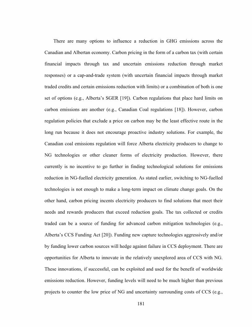
181

There are many options to influence a reduction in GHG emissions across the

Canadian and Albertan economy. Carbon pricing in the form of a carbon tax (with certain

financial impacts through tax and uncertain emissions reduction through market

responses) or a cap-and-trade system (with uncertain financial impacts through market

traded credits and certain emissions reduction with limits) or a combination of both is one

set of options (e.g., Alberta’s SGER [19]). Carbon regulations that place hard limits on

carbon emissions are another (e.g., Canadian Coal regulations [18]). However, carbon

regulation policies that exclude a price on carbon may be the least effective route in the

long run because it does not encourage proactive industry solutions. For example, the

Canadian coal emissions regulation will force Alberta electricity producers to change to

NG technologies or other cleaner forms of electricity production. However, there

currently is no incentive to go further in finding technological solutions for emissions

reduction in NG-fuelled electricity generation. As stated earlier, switching to NG-fuelled

technologies is not enough to make a long-term impact on climate change goals. On the

other hand, carbon pricing incents electricity producers to find solutions that meet their

needs and rewards producers that exceed reduction goals. The tax collected or credits

traded can be a source of funding for advanced carbon mitigation technologies (e.g.,

Alberta’s CCS Funding Act [20]). Funding new capture technologies aggressively and/or

by funding lower carbon sources will hedge against failure in CCS deployment. There are

opportunities for Alberta to innovate in the relatively unexplored area of CCS with NG.

These innovations, if successful, can be exploited and used for the benefit of worldwide

emissions reduction. However, funding levels will need to be much higher than previous

projects to counter the low price of NG and uncertainty surrounding costs of CCS (e.g.,

182

failures of Swan Hills Synfuels project [21], and Project Pioneer retrofit of the Keephills

3 SCPC power plant due to unfavourable economics [22]).

The widespread relinquishment of North America’s coal’s production share to NG

technologies, in absence of large scale RET deployment, may eventually stress the supply

of NG resulting in higher NG prices [23][24]. Flexible carbon policy maybe required that

takes into account the variability of NG prices as shown in this analysis. Increasing NG

use can also drive upstream GHG emissions to increase due to the extraction and

transportation, which can be exacerbated by the increase in nonconventional supplies

[25]. This has been demonstrated in this case study, but has also been suggested by others

[25]. Additionally, the increase in NG for power generation reduces the supply and

potentially increases prices to other industries and consumers, resulting in the possibility

that environmentally beneficial fuel switching may become uneconomic (e.g.,

transportation technologies using diesel rather than NG). Policy-makers when setting

long term goals should consider the combined upstream GHG emissions and possible

knock-on effects of dramatic NG consumption increases due to fuel switching in power

generation.

Using the results from the Framework, the case study proposes an answer to the

question; “Is switching to NG fired generation technologies an effective long term GHG

reduction plan?” The answer to this question seems apparent at first glance: the

reductions achieved by switching to NG are substantial (approximately 40% reduction

from S1), especially in light of the failure of CCS adoption in coal technologies in

Alberta. The future addition of CCS technologies in NGCC promises even further

183

reduction. In order to make the adoption of NGCC CCS technology a reality, much

stronger carbon policy and financial incentives are needed.

3.2 Implications for LCA Studies

The contribution from this study is that it provides a framework for analysts to

evaluate advanced carbon capture technologies that takes into account the system-wide

implications of CCS use, including the life cycle costs and life cycle emissions, and the

uncertainty inherent in the analysis. The framework uses Energy System Modeling

(ESM), Life Cycle Costing (LCC), and Life Cycle Assessment (LCA) as tools to inform

the uncertainty assessment component of the framework. A large portion of the

contribution to the field is made by providing methods of exploring the effect of

parameter probability distribution variability and alternative scenarios on GHG emissions

and cost results. This is done with the uncertainty assessment model’s three main

components; Deterministic Sensitivity Analysis, Uncertainty Analysis, and Stochastic

Sensitivity Analysis.

The use of the Contribution and Perturbation Analyses in the Deterministic

Sensitivity Analysis provide an informative visual indication of the relative influence

various generation system technologies and parameters have on the deterministic results

that are presented. Insights into the requirements of data quality (i.e., important

parameters require robust data for the development of probability distributions), and

treatment (i.e., other analysis may be required to frame the uncertainty in qualitative

terms (e.g., scenarios)) for use in subsequent analyses are obtained. Additionally, in the

situation where the number of parameters is high, the Perturbation Analysis can be used

184

to pick the most influential and create a target list of parameters to investigate further,

thereby saving considerable effort by reducing research on less important parameters.

Through the use of Uncertainty Propagation Analysis [26][27], using a Monte

Carlo Simulation [28] sampling method, the uncertainty in overall system wide results is

estimated resulting in cost and environmental performance outcomes expressed as

probability distributions for each scenario. Comparing cumulative CO2 emissions

probability distributions across the scenarios assesses their relative performance in

reducing GHG emissions over the period of the simulation. The performance of

individual scenarios is assessed by determining the probability of achieving the GHG

emissions reduction goals set out in various climate change policies (i.e., Alberta’s goal

of -14% of 2005 levels). This Uncertainty Analysis also provides a means to go beyond

point estimates by quantifying the results in terms of significance using a 95% confidence

interval. Ranking of the alternatives is achievable by resolving scenario distribution

results using a Discernibility Analysis [26][27], which allows for direct numerical

comparisons. This analysis provides the analyst the means to quantify the difference

between mature and immature technologies.

Considering that researchers are faced with challenges in gathering data,

especially for emerging technologies, a set of analyses within a Stochastic Sensitivity

Analysis are developed to test the assumptions made in developing the probability

distributions. Sparse data, or a lack of knowledge about the nature of the parameter’s

uncertainty, can lead to arbitrary or general distribution representation, which in turn

degrades the robustness of the results. A Probability Distribution Scenario Analysis uses

probability distribution characteristics and the constructs of scenarios to frame the

185

uncertainty in parameters of interest. A Probability Distribution Type Sensitivity

Analysis assesses the impacts of choosing different distribution types on the overall

results of the Uncertainty Analysis. In the case where severe effects are seen, the

researcher could re-evaluate the development of the distribution, gather more data to

develop the distributions further, or present the overall results with the complimentary

stochastic sensitivity results. In addition to the distribution types chosen to characterize

the parameters, the parameter distributions may not accurately reproduce a bias to either

extreme in the ranges explored in the uncertainty analysis. A Relative Degree of

Optimism (RDO) Analysis is conducted to explore the effects of skew (RDO) on the

overall results. Additionally, in the case where a theoretical breakthrough technology is

assessed (as in the case study), this method provides a means to assess the improvement

required to meet a significant threshold (i.e., what performance or cost is required to have

a 95% confidence in out performing an alternative).

Assessing the improvement in technology over time may be of importance when

looking at long time frames. A simple method was proposed to investigate the effects of

technology introduction time and technology improvement on the cost and performance

results. Modifying the method established in the Relative Degree of Optimism Analysis

(i.e., through using beta distributions to manipulate the probability distributions) allowed

for a simple inverse relationship to be established between temporal and cost and

performance parameters. In this way, researchers can explore the uncertainty surrounding

optimal timing of emerging technologies. As a policy-maker, an estimate of the optimal

time (or conversely, point-of-no-return) to introduce a future theoretical technology can

be made. These methods also provide the researcher with additional information on the

186

effects of imprecisely represented parameters by indicating the conditions (i.e., through

parameter distribution characteristics) that change the relative ranking of alternatives.

Finally, this thesis presents a Combined Sensitivity and Uncertainty Propagation

Analysis. This analysis provides a means of systematically assessing the effects of

parameters that highly affect the overall results, while still maintaining the uncertainty

propagation methods presented above. It provides the conditions under which scenario

rankings would change, and provides insight into the policies required to achieve the

desired ranking (i.e., through carbon tax). This analysis also provides insight into the risk

of inconstant parameter values (e.g., NG prices fluctuate over time) and the resulting

change in opposing parameters required to compensate for rank maintenance (i.e.,

increase in carbon tax to maintain economic attractiveness of CCS).

The contribution from this study is applicable to the larger field of LCA in that it

provides more detailed assessment of the effects of uncertainty than current studies and

pushes the methods for quantifying and incorporating uncertainty into decision-making

contexts. The methods used and the framework proposed provides a means to more

accurately assess, quantify, and incorporate uncertainty in into LCA studies of other

emerging energy technologies.

3.3 Implications for Policy

The considerable additional costs associated with CCS implies that government

policies (e.g., subsidies, tax credits, loans) are required to assist the demonstration and

deployment of the technology in a timely manner. Unless there is a very high carbon tax,

early CCS plants will be very expensive and will not be competitive with conventional

187

power facilities (e.g., [21][22]). The proposed framework can be used to evaluate

advanced capture technology (and by extension other advanced energy technologies) for

use in a system-wide application. An evaluation focused on the characteristics (e.g.,

energy requirements, capital and operating costs, and environmental performance) and

risks (e.g., economic and environmental) associated with the advanced capture

technology can provide decision-makers in industry valuable information required to

make informed decisions about investment choices. These tools can also inform decision-

makers in government in order to make effective policies that influence and encourage

industry choices that help to meet GHG targets.

4 Considerations for Future Work

The design of the Framework is very dependent on computing resource intensive

MATLAB [29] coding to execute the operation of the routines and methods described for

both components. For example, the execution of the Combined Sensitivity and

Uncertainty Propagation Analysis requires over 36 hours of computational time to

generate 400 MCS executions (a 20x20 matrix) with 10000 samples per execution.

Future effort into improving the efficiency of the code would help reduce the computing

effort and time required to complete the full set of analyses presented. The current coding

uses “for loops” extensively to execute the Monte Carlo Simulation sampling routines,

which could be replaced with more matrix-based operations to aid in this effort. In

addition to more efficient coding, the use of Latin Hypercube or Hammersley sampling

methods could also improve efficiency and the potential accuracy of the sampling,

depending on the number of samples performed or the computational time available for

the analysis.

188

Another area of future work involves more options for the calculation of fuel

prices over time. Currently, fuel price is set to a constant value for the given time period

of the analysis. An improved method would involve the setting of fuel price for each year

of the analysis, to account for year-to-year price fluctuations, or for price escalation due

to supply-demand economics (i.e., increase NG use in power generation reduces supply).

In a more involved improvement, the Integrated Life Cycle Model could be

reworked to involve more dynamic effects; such as technology choice trends based on

fuel price or carbon policy impacts. Such a model was built by McFarland et al. [30] in

their study on representing energy technologies using top-down economic models with

bottom-up information. They were able to simulate the switching from NG technologies

to coal when NG price increased due to demand increase. This would be a useful addition

to the model since information regarding risk in advanced CCS technology

implementation in long time frames would be valuable to decision-makers (e.g., building

technologies that maybe the most expensive option due to future fuel cost).

Another area of future work involves the improvement of the LCA aspects of the

Integrated LC Model. The scope of the life cycle impacts considered could be expanded

to include material flows related to the building and demolition of plants and manufacture

and disposal of chemicals used in the CO2 capture process. In addition, other impacts

such as resource depletion, acidification, and land use could also be included. These LC

additions would add to the information available about the system wide implications and

trade-offs related to CCS technology use, in a way that more fully captures other

potential pitfalls or benefits of potential GHG mitigation pathways.

189

The selection of probability distribution and range of important data (e.g., NG

price) matters to the qualitative conclusions that are derived from the

analysis. Therefore, there is a need for future work in this area to improve on the

applicability of the results used for decision-making. This study provides a means of

addressing the importance of parameter ranges and distributions, however future work

could improve this further. For example, where as this study assumed all investigated

parameters are independent, a new model including subjective probabilities to link certain

parameters could be developed to more accurately represent reality. Examples would be

linking the costs and performance of technology with time, or the share of technology

based on the price of fuel.

Finally, the framework could be modified and adapted to assess other uncertain

emerging technologies such as advanced RET or nuclear technologies. Similarly, the

framework could be applied to a greater region, such as Canada, and assess a more

diversified mix of technologies. The Uncertainty Assessment Model could also be

adapted to accept data from other models that assess technologies from other sectors,

such as oil and gas, and transportation.

The additional information from the above improvements will add to the holistic

information on the implications of CCS deployed at scale and system wide. It will allow

for further reflection on the complexity involved in using the technology. For example it

may help decision-makers assess the potential for beneficial economies of scale or

detrimental material resource constraints.

190

5 Significance of the Research

The framework contributes to the international field of LCA and can be used to

evaluate an emerging CCS technology and can be adapted more broadly to a range of

energy system investment decisions. This thesis contributes by going beyond point

estimates or ranges of performance by presenting uncertainty in environmental

performance and cost results as probability distributions. These tools can help to uncover

the trade-offs (e.g., capturing CO2 at the expense of efficiency and additional cost) that

must be faced to achieve a stated set of objectives (e.g., emissions reduction targets). The

framework improves on existing analyses by allowing for a more thorough assessment of

outcomes (e.g., through associated probabilities, and the effects of data quality),

consequences and risks than currently exists. The framework can aid in determining

effective strategies for developing and deploying cleaner and more efficient energy

technologies while being cognizant of the economic costs. It can provide governments

with the information required to develop incentives required for the technologies to be

deployed in the timeframe required to reduce the impacts from GHG emissions.

191

References

[1] R. Sathre, M. Chester, J. Cain, and E. Masanet, "A framework for environmental assessment of CO2 capture and storage systems," Energy, vol. 37, no. 1, pp. 540-548, Feb 01 2012.

[2] H. Lund and B. V. Mathiesen, "The role of Carbon Capture and Storage in a future sustainable energy system," Energy, vol. 44, no. 1, pp. 469-476, Aug 01 2012.

[3] P. Jaramillo, W. M. Griffin, and H. S. Matthews, "Comparative Life-Cycle Air Emissions of Coal, Domestic Natural Gas, LNG, and SNG for Electricity Generation," Environmental Science & Technology, vol. 41, no. 17, pp. 6290-6296, Sep 2007.

[4] M. Pehnt and J. Henkel, "Life cycle assessment of carbon dioxide capture and storage from lignite power plants," International Journal of Greenhouse Gas Control, vol. 3, no. 1, pp. 49-66, Feb 2009.

[5] C.-C. Cormos, "Integrated assessment of IGCC power generation technology with carbon capture and storage (CCS)," Energy, vol. 42, no. 1, pp. 434-445, Jul 01 2012.

[6] N. A. Odeh and T. T. Cockerill, "Life cycle GHG assessment of fossil fuel power plants with carbon capture and storage," Energy Policy, vol. 36, no. 1, pp. 367-380, 2008.

[7] H. Zhai and E. S. Rubin, "A Techno-Economic Assessment of Polymer Membrane Systems for Post-combustion Carbon Capture at Coal-fired Power Plants," Environmental Science & Technology, no., pp. 130213162018003, Mar 13 2013.

[8] U.S. Department of Energy’s National Energy Technology Laboratory, "Life Cycle Analysis: Natural Gas Combined Cycle (NGCC) Power Plant," U.S. Department of Energy’s National Energy Technology Laboratory, Sep 30 2010.

[9] E. S. Rubin, C. Chen, and A. B. Rao, "Cost and performance of fossil fuel power plants with CO2 capture and storage," Energy Policy, vol. 35, no. 9, pp. 4444-4454, 2007.

[10] P. Versteeg and E. S. Rubin, "Technical and economic assessment of ammonia-based post-combustion CO2 capture," Energy Procedia, vol. 4 IS -, no., pp. 1957-1964, 2011.

[11] E. S. Rubin and H. Zhai, "The Cost of Carbon Capture and Storage for Natural Gas Combined Cycle Power Plants," Environmental Science & Technology, vol. 46, no. 6, pp. 3076-3084, Apr 20 2012.

[12] G. F. Nemet, E. Baker, and K. E. Jenni, "Modeling the future costs of carbon capture using experts&apos; elicited probabilities under policy scenarios," Energy, vol. 56, no. 0, pp. 218-228, Jul 2013.

[13] K. Johnsen, K. Helle, and T. Myhrvold, "Scale-up of CO2 capture processes: The role of Technology Qualification," Greenhouse Gas Control Technologies 9 Proceedings of the 9th International Conference on Greenhouse Gas Control Technologies (GHGT-9), 16–20 November 2008, Washington DC, USA, vol. 1, no. 1, pp. 163-170, Mar 01 2009.

192

[14] V. Rai, D. G. Victor, and M. C. Thurber, "Carbon capture and storage at scale: Lessons from the growth of analogous energy technologies," Energy Policy, vol. 38, no. 8, pp. 4089-4098, Aug 2010.

[15] H. J. Herzog, "Scaling up carbon dioxide capture and storage: From megatons to gigatons," Energy Economics, vol. 33, no. 4, pp. 597-604, Jul 01 2011.

[16] E. S. Rubin, H. Mantripragada, A. Marks, P. Versteeg, and J. Kitchin, "The outlook for improved carbon capture technology," Progress in Energy and Combustion Science, vol. 38, no. 5, pp. 630-671, 2012.

[17] E. S. Rubin, S. Yeh, M. Antes, M. Berkenpas, and J. Davison, "Use of experience curves to estimate the future cost of power plants with CO2 capture," International Journal of Greenhouse Gas Control, vol. 1, no. 2, pp. 188-197, 2007.

[18] Government of Canada, "Reduction of Carbon Dioxide Emissions from Coal-fired Generation of Electricity Regulations (SOR/2012-167), Canadian Environmental Protection Act, 1999," Government of Canada, ed. Ottawa, Ontario: Minister of Justice, 2012.

[19] Government of Alberta, "Climate Change and Emissions Management Act: Specified Gas Emitters Regulation," Government of Alberta, ed. Edmonton, Alberta: Alberta Queen's Printer, 2007.

[20] Government of Alberta, "Carbon Capture and Storage Funding Act," Government of Alberta, ed. Edmonton, Alberta: Alberta Queens Printer, 2009.

[21] R. Blackwell. (2013). Alberta cancels funding for carbon capture project. The Globe and Mail, 2013 [Online]. Available: http://www.theglobeandmail.com/report-on-business/industry-news/energy-and-resources/alberta-cancels-funding-for-carbon-capture-project/article9024237/ accessed on 21 September 2013

[22] C. Tait. (2013). Alberta's carbon capture efforts set back. The Globe and Mail, 2012 [Online]. Available: http://www.theglobeandmail.com/report-on-business/industry-news/energy-and-resources/albertas-carbon-capture-efforts-set-back/article4103684/ accessed on 21 September, 2013

[23] D. Simbeck and D. Beecy, "The CCS paradox: The much higher CO2 avoidance costs of existing versus new fossil fuel power plants," Greenhouse Gas Control Technologies 9 Proceedings of the 9th International Conference on Greenhouse Gas Control Technologies (GHGT-9), 16–20 November 2008, Washington DC, USA, vol. 4, no. 0, pp. 1917-1924, 2011.

[24] National Energy Board, "Natural Gas for Power Generation," Jul 012006. [25] R. W. Howarth, R. Santoro, and A. Ingraffea, "Methane and the greenhouse-gas

footprint of natural gas from shale formations," Climatic Change, vol. 106, no. 4, pp. 679-690, May 12 2011.

[26] J. Clavreul, D. Guyonnet, and T. H. Christensen, "Quantifying uncertainty in LCA-modelling of waste management systems," Waste Management, vol. 32, no. 12, pp. 2482-2495, Dec 2012.

[27] R. Heijungs and R. Kleijn, "Numerical approaches towards life cycle interpretation five examples," The International Journal of Life Cycle Assessment, vol. 6, no. 3, pp. 141-148, Jun 01 2001.

193

[28] M. G. Morgan, M. Henrion, and M. Small, Uncertainty: A Guide to Dealing with Uncertainty in Quantitative Risk and Policy Analysis. Cambridge, UK: Cambridge University Press, 2003.

[29] "MATLAB," 2013b ed. Natick, Massachusetts: The Mathworks Inc, 2013. [30] J. R. McFarland, J. Reilly, and H. J. Herzog, "Representing Energy Technologies

in Top-down Economic Models Using Bottom-up Information," MIT Joint Program on the Science and Policy of Global Change, Cambridge, MA, Oct 2002.

194

APPENDIX A: Data Tables

Table 5-1: Power Plant Specifications from IECM v8.0.2

Specification PC SCPC SCPC CCS NGCC NGCC

CCS NGSC Cogen

Turbine Type N/A N/A N/A GE 7FB GE 7FB GE 7EA GE LM6000

Net Heat Rate (kJ/kWh)

10428 9786 14235 7200 Variable 9800 12600

Capacity Factor 0.9 0.9 0.9 Variable Variable 0.2 0.85

Gross Output (MW)

500 500 500 908.7 842.9 50 90

Net Output (MW) 457 460 391 527 Variable 45 85

CO2 Emissions (kg/kWh)

0.9809 0.9206 0.1340 0.3642 Variable 0.5000 0.2410

CO2 Captured (kg/kWh)

N/A N/A 1.206 N/A Variable N/A N/A

Fixed Cost ($/kW) 33.9 34.5 50.3 10.2 17.1 12.6 13.7

Variable Cost ($/MWh)

4.0 3.7 7.7 0.7 Variable 4.2 4.2

Capital Required ($/kW net)

2118 2192 4094 842 842 1050 1800

CCS Capital Required ($/kW net)

N/A N/A 1141 N/A Variable N/A N/A

CCS Fixed Cost ($/kW)

N/A N/A 15.4 N/A 2.237 N/A N/A

CCS Variable Cost ($/MWh)

N/A N/A 20.2 N/A Variable N/A N/A

Fuel HHV (kJ/Kg) 17780 17780 17780 52290 52290 52290 52290

Project Life 30 30 30 30 30 30 30

195

Table 5-2: Parameters used in the Contribution Analysis Parameters Description Value Availability Time of Advanced CCS Technology

The availability time, or introduction time, of an advanced CCS technology for NGCC.

20 years

Capture Technology Capital The additional capital required for the advanced NGCC CCS technology.

$545/kWnet

Carbon Capture and Processing Parasitic Power

The power requirements for carbon capture and processing, or parasitic power of the advanced NGCC CCS technology.

12.9%

CO2 Removal Efficiency The CO2 removal efficiency of the future advanced CCS technology.

91.25%

Retrofit Period The retrofit period is the time that it takes to retrofit all existing NGCC plants with CCS.

20 years

Variable O&M The variable O&M required to operate an NGCC plant with the advanced CCS technology. Excludes fuel and carbon tax costs.

$5.96/MWh

CCS Capital Cost Penalty The penalty to the CCS technology capital cost for a retrofitted plant.

1.5

Capacity Factor of NGCC Plants

The capacity factor of an NGCC power plant.

65%

Carbon Tax The imposed carbon tax. $10/tonne

LC Emissions of NG Extraction

The upstream emissions (per GJ of fuel consumed) of natural gas extraction and transportation to the power plant.

10.8 kg/GJ

Capital Recovery Factor (CRF)

The capital recovery factor used to calculate the levelized cost of electricity for all plants.

12.2%

NG Price The price of NG. $6/GJ

196

Table 5-3: Parameter Values used for the Perturbation Analysis

Parameter Perturbation

Baseline +5% -5%

CO2 Removal Efficiency (ratio) 0.9125 0.95813 0.86687

CO2 Removal Power Requirements (ratio)

0.12862 0.13506 0.12219

Upstream Emissions of NG (g/GJ) 10795 11335 10255

Availability of Technology (years) 20 21 19

Retrofit Period (years) 20 21 19

CCS Capital Required ($/kWnet) 545.12 572.38 517.87

CCS Variable O&M Required ($/MWh) 5.4 5.67 5.13

Carbon Tax ($/tonne) 10 10.5 9.5

NG Price ($/GJ) 6 6.3 5.7

CRF (ratio) 0.1215 0.12757 0.11542

Capacity Factor (ratio) 0.65 0.6825 0.6175

Retrofit Capital Penalty (ratio) 1.5 1.575 1.425

197

Table 5-4: Technology Parameter Baseline Distributions

Technology Parameter

Baseline Distribution

Type Mean SD Lower Limit Upper Limit

Availability Time of Advanced CCS Technology (Years)

Discrete Uniform 30 11.5 10 50

Retrofit Period (Years) Discrete Uniform 20 5.76 10 30

Capital ($/kWh) Uniform 545 45.0 467 623 Carbon Capture and Processing Parasitic Power (%)

Uniform 12.9 1.02 11.0 14.7

Variable O&M ($/MWh) Uniform 5.40 0.34 4.62 6.14

CO2 Removal Efficiency (%) Beta (a, b = 2) 91.25 0.4 90 92.5

Capacity Factor of NGCC Plants (%) Beta (a, b = 2) 65 8.3 40 90

Retrofit Penalty Beta (a, b = 2) 1.5 0.05 1 2

Table 5-5: System Parameter Baseline Distributions

System Parameter Baseline

Distribution Type Mean SD Lower Limit Upper Limit

NG Price ($/GJ) (Stable)

Beta (a=16, b=21.3) 6 0.56 3 10

NG Price ($/GJ) (Unstable)

Beta (a=2, b=2.66) 6 1.46 3 10

LC Emissions of NG Extraction and Transportation (g/GJ)

Normal 10795 1402 6589 15001

Capital Recovery Factor (%) Uniform 12 0.60 11

(0.3 Percentile) 13

(97.7 Percentile)