UC BerkeleyHaas School of Business

Economic Analysis for Business Decisions(EWMBA 201A)

Game Theory IIIApplications (part 2)

Lectures 8-9Sep. 19, 2009

Outline

[1] Midterm

[2] Strictly competitive games and maximinzation

[3] Oligopolistic competition — the main ideas

[4] Auctions

[5] Bargaining / negotiations

[6] Observational learning — open discussion (if time permits)

Strictly competitive games

In strictly competitive games, the players’ interests are diametrically op-posed, like in Bertrand’s duopoly game.

More precisely, a strategic two-player game is strictly competitive if for anytwo outcomes a and b we have

a %1 b if and only if b %2 a.

A strictly competitive game can be represented as a zero-sum game

L RT A,−A B,−BB C,−C D,−D

This class of games is important for a number of reasons:

— A simple decision making procedure leads each player to choose a Nashequilibrium action.

— Unfortunately, there are innumerable social and economic situationswhich are strictly competitive.

— In the game of business, a successful strategy is avoiding the zero-sumgames by reshaping the game.

=⇒ See, Brandenburger and Nalebuff, and Hermalin (Chapter 6).

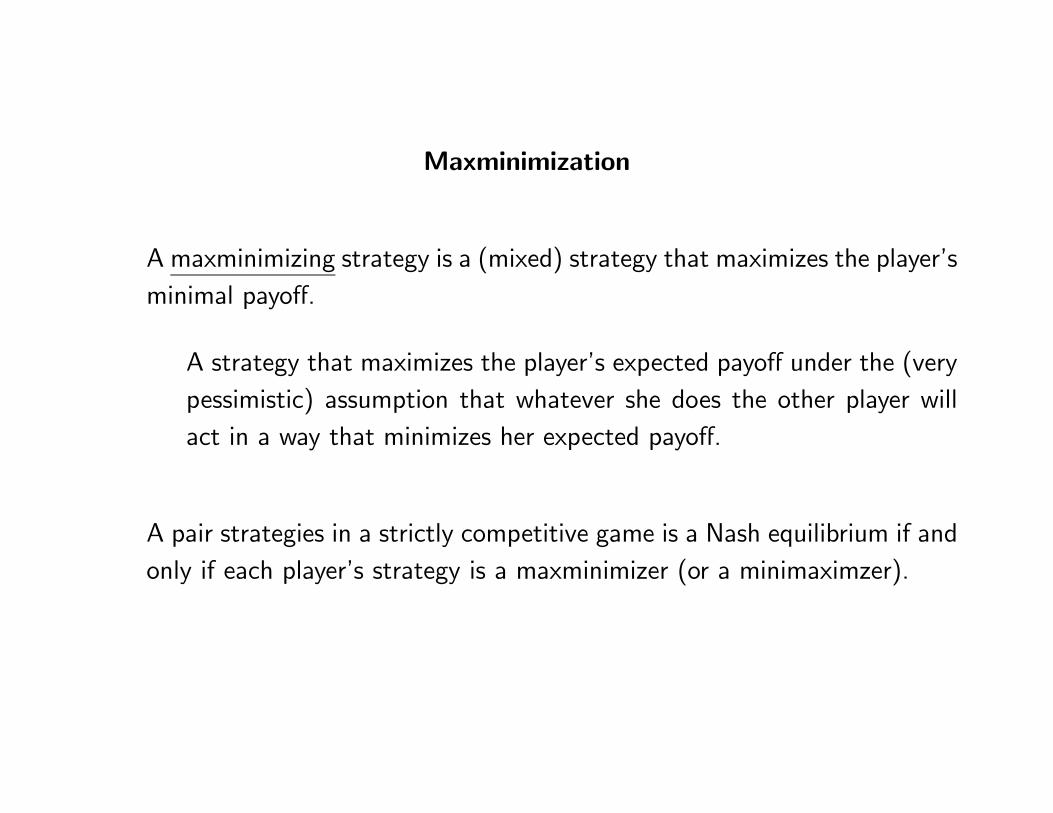
Maxminimization

A maxminimizing strategy is a (mixed) strategy that maximizes the player’sminimal payoff.

A strategy that maximizes the player’s expected payoff under the (verypessimistic) assumption that whatever she does the other player willact in a way that minimizes her expected payoff.

A pair strategies in a strictly competitive game is a Nash equilibrium if andonly if each player’s strategy is a maxminimizer (or a minimaximzer).

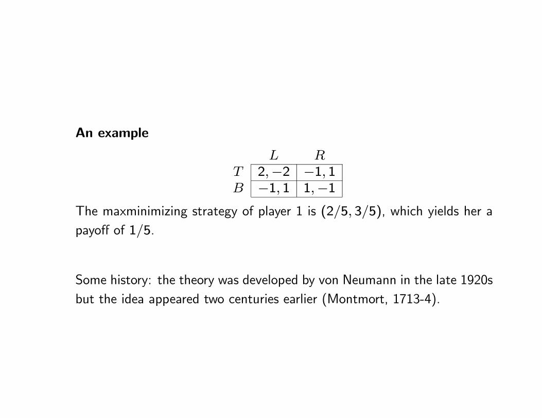
An example

L RT 2,−2 −1, 1B −1, 1 1,−1

The maxminimizing strategy of player 1 is (2/5, 3/5), which yields her apayoff of 1/5.

Some history: the theory was developed by von Neumann in the late 1920sbut the idea appeared two centuries earlier (Montmort, 1713-4).

Review of oligopolistic competition

• In an oligopolistic market, a small number of firms compete for the businessof consumers.

• Barriers to entry restrict the number of firms, possibly allowing firms toearn substantial profits.

• In models of oligopoly, decisions involve strategic considerations — eachfirm must best response to the actions of its rivals.

Cournot’s model

— Firms produce a homogeneous good, and all firms decide simultane-ously how much to produce.

— Each firm chooses a profit-maximizing output, treating the outputs ofits rivals as fixed.

— In the Nash equilibrium, each firm’s profit is higher (resp. lower) thanit is under perfect competition (resp. collusion).

Stackelberg’s model

— Firms move sequentially so we use backward induction to find a sub-game perfect equilibrium.

— The firm that sets its output first has a strategic advantage and earnsa higher profit in equilibrium.

— Which model, Cournot or Stackelberg, is more appropriate depends onthe industry (operating advantage / leadership position).

Bertrand’s model

— Cournot

Each firm chooses an output, and the price is determined by the marketdemand in relation to the total output produced.

— Bertrand

Each firm chooses a price, and produces enough output to meet thedemand it faces, given the prices chosen by all the firms.

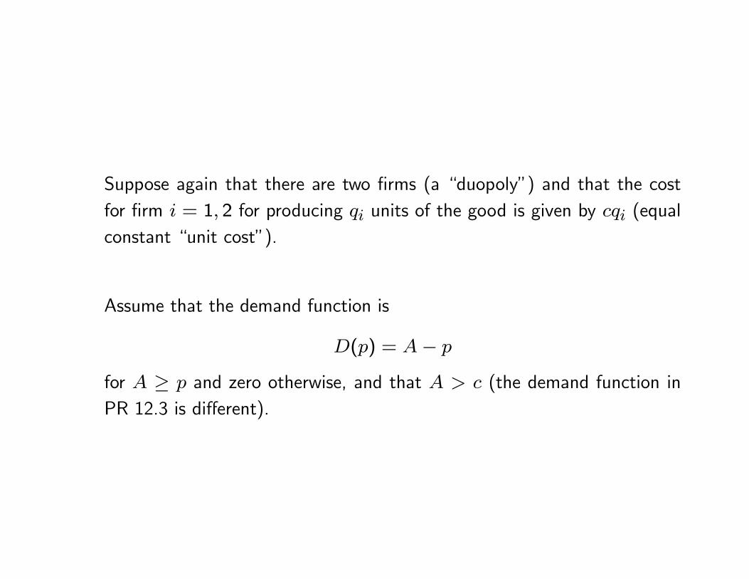
Suppose again that there are two firms (a “duopoly”) and that the costfor firm i = 1, 2 for producing qi units of the good is given by cqi (equalconstant “unit cost”).

Assume that the demand function is

D(p) = A− p

for A ≥ p and zero otherwise, and that A > c (the demand function inPR 12.3 is different).

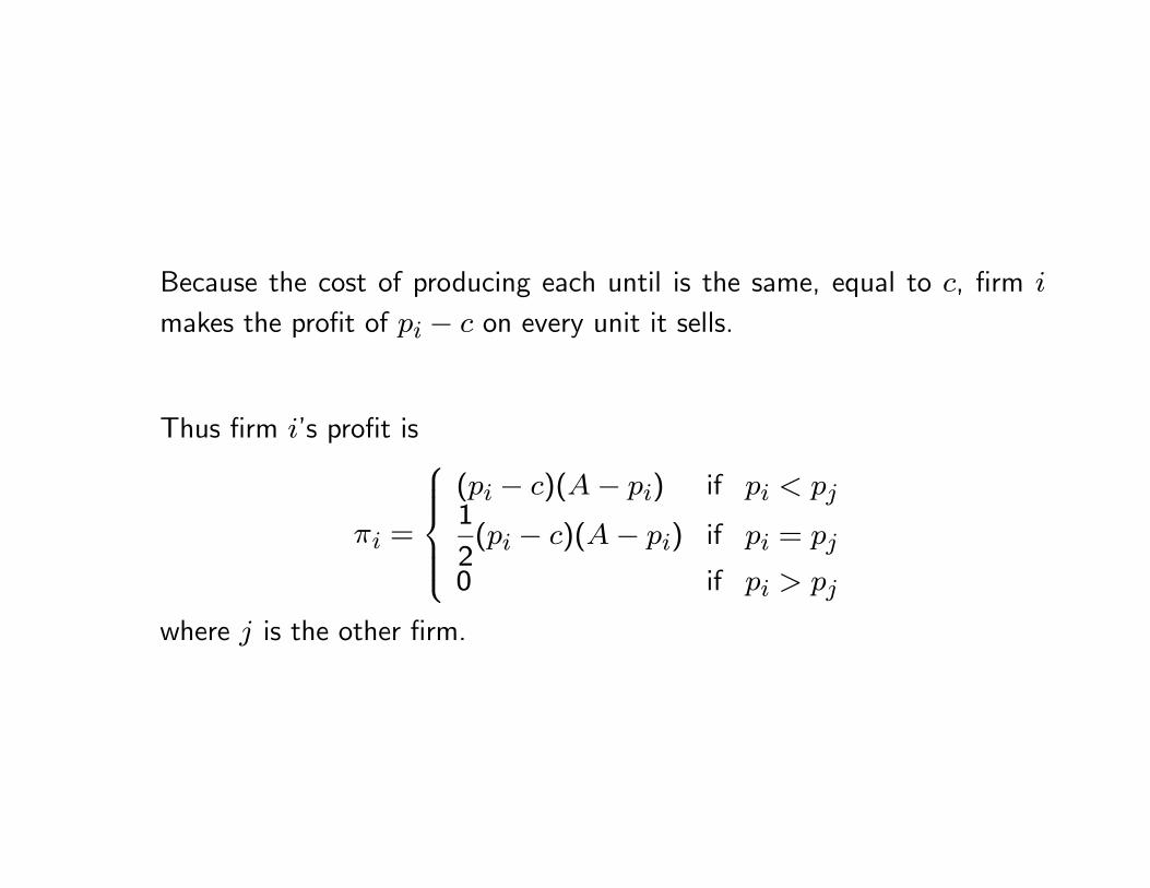
Because the cost of producing each until is the same, equal to c, firm i

makes the profit of pi − c on every unit it sells.

Thus firm i’s profit is

πi =

⎧⎪⎪⎪⎨⎪⎪⎪⎩(pi − c)(A− pi) if pi < pj1

2(pi − c)(A− pi) if pi = pj

0 if pi > pj

where j is the other firm.

The unique subgame perfect equilibrium is (p1, p2) = (c, c):

— If one firm charges the price c, then the other firm can do no betterthan charge the price c.

— If p1 > c and p2 > c, then each firm i can increase its profit bylowering its price pi slightly below pj.

=⇒ Cournot: the market price decreases toward c (zero profits) as the numberof firms increases.

=⇒ Bertrand: the price is c even if there are only two firms (and the priceremains c when the number of firm increases).

Auctions (PR 13.8)

From Babylonia to eBay, auctioning has a very long history.

• Babylon:

- women at marriageable age.

• Athens, Rome, and medieval Europe:

- rights to collect taxes,

- dispose of confiscated property,

- lease of land and mines,

and more...

The word “auction” comes from the Latin augere, meaning “to increase.”

The earliest use of the English word “auction” given by the Oxford EnglishDictionary dates from 1595 and concerns an auction “when will be soldSlaves, household goods, etc.”

In this era, the auctioneer lit a short candle and bids were valid only ifmade before the flame went out — Samuel Pepys (1633-1703) —

• Auctions, broadly defined, are used to allocate significant economics re-sources.

Examples: works of art, government bonds, offshore tracts for oil ex-ploration, radio spectrum, and more.

• Auctions take many forms. A game-theoretic framework enables to under-stand the consequences of various auction designs.

• Game theory can suggest the design likely to be most effective, and theone likely to raise the most revenues.

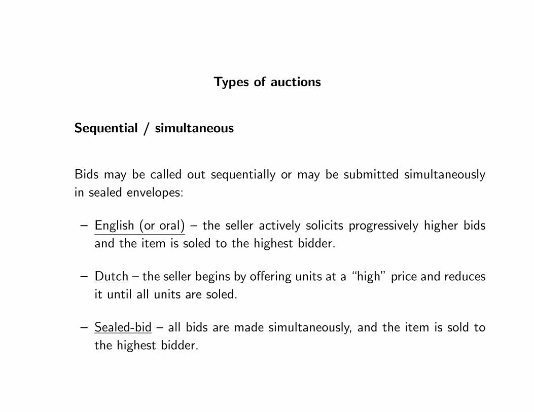
Types of auctions

Sequential / simultaneous

Bids may be called out sequentially or may be submitted simultaneouslyin sealed envelopes:

— English (or oral) — the seller actively solicits progressively higher bidsand the item is soled to the highest bidder.

— Dutch — the seller begins by offering units at a “high” price and reducesit until all units are soled.

— Sealed-bid — all bids are made simultaneously, and the item is sold tothe highest bidder.

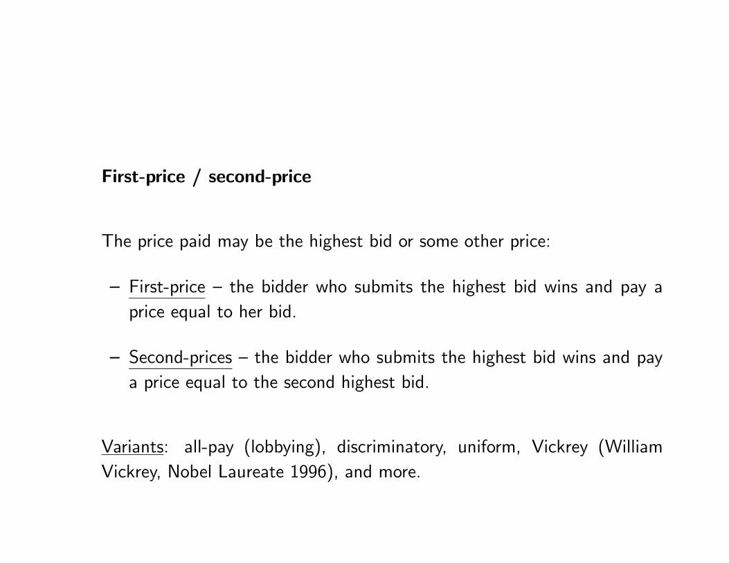
First-price / second-price

The price paid may be the highest bid or some other price:

— First-price — the bidder who submits the highest bid wins and pay aprice equal to her bid.

— Second-prices — the bidder who submits the highest bid wins and paya price equal to the second highest bid.

Variants: all-pay (lobbying), discriminatory, uniform, Vickrey (WilliamVickrey, Nobel Laureate 1996), and more.

Private-value / common-value

Bidders can be certain or uncertain about each other’s valuation:

— In private-value auctions, valuations differ among bidders, and eachbidder is certain of her own valuation and can be certain or uncertainof every other bidder’s valuation.

— In common-value auctions, all bidders have the same valuation, butbidders do not know this value precisely and their estimates of it vary.

First-price auction (with perfect information)

To define the game precisely, denote by vi the value that bidder i attachesto the object. If she obtains the object at price p then her payoff is vi−p.

Assume that bidders’ valuations are all different and all positive. Numberthe bidders 1 through n in such a way that

v1 > v2 > · · · > vn > 0.

Each bidder i submits a (sealed) bid bi. If bidder i obtains the object, shereceives a payoff vi − bi. Otherwise, her payoff is zero.

Tie-breaking — if two or more bidders are in a tie for the highest bid, thewinner is the bidder with the highest valuation.

In summary, a first-price sealed-bid auction with perfect information is thefollowing strategic game:

— Players: the n bidders.

— Actions: the set of possible bids bi of each player i (nonnegative num-bers).

— Payoffs: the preferences of player i are given by

ui =

(vi − b̄ if bi = b̄ and vi > vj if bj = b̄0 if bi < b̄

where b̄ is the highest bid.

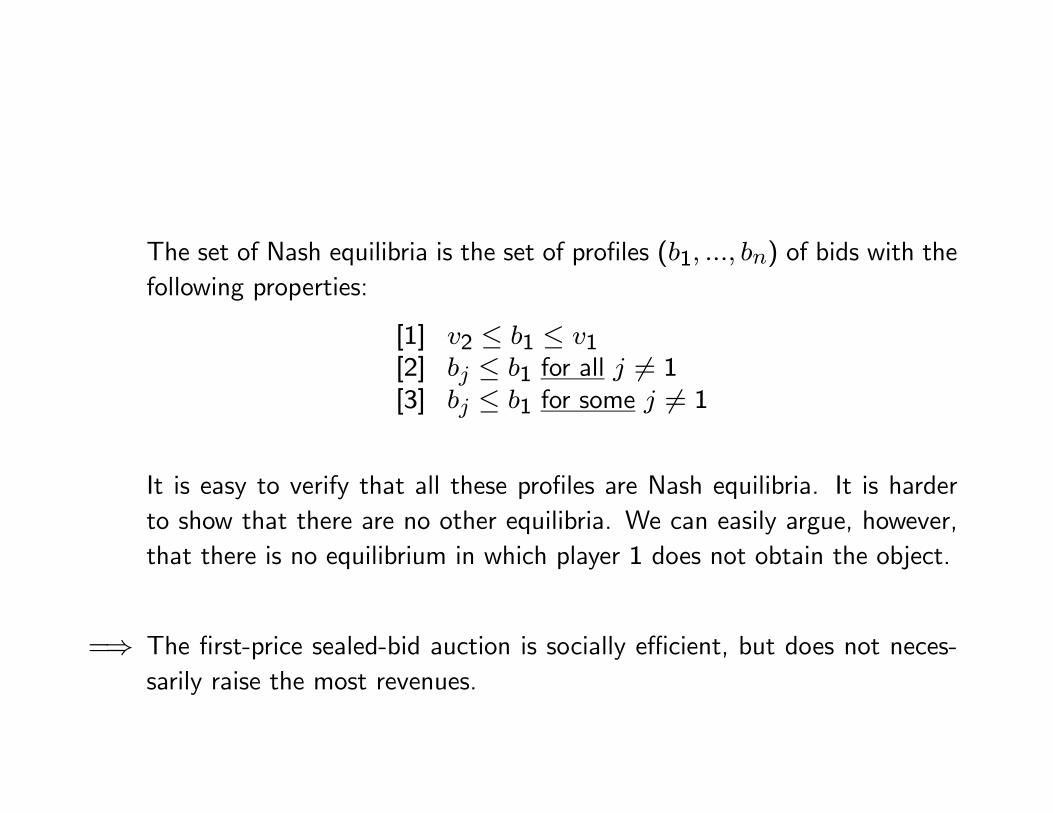
The set of Nash equilibria is the set of profiles (b1, ..., bn) of bids with thefollowing properties:

[1] v2 ≤ b1 ≤ v1[2] bj ≤ b1 for all j 6= 1[3] bj ≤ b1 for some j 6= 1

It is easy to verify that all these profiles are Nash equilibria. It is harderto show that there are no other equilibria. We can easily argue, however,that there is no equilibrium in which player 1 does not obtain the object.

=⇒ The first-price sealed-bid auction is socially efficient, but does not neces-sarily raise the most revenues.

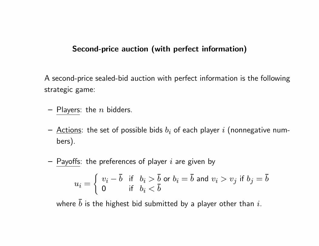
Second-price auction (with perfect information)

A second-price sealed-bid auction with perfect information is the followingstrategic game:

— Players: the n bidders.

— Actions: the set of possible bids bi of each player i (nonnegative num-bers).

— Payoffs: the preferences of player i are given by

ui =

(vi − b̄ if bi > b̄ or bi = b̄ and vi > vj if bj = b̄0 if bi < b̄

where b̄ is the highest bid submitted by a player other than i.

First note that for any player i the bid bi = vi is a (weakly) dominantaction (a “truthful” bid), in contrast to the first-price auction.

The second-price auction has many equilibria, but the equilibrium bi = vifor all i is distinguished by the fact that every player’s action dominatesall other actions.

Another equilibrium in which player j 6= 1 obtains the good is that inwhich

[1] b1 < vj and bj > v1[2] bi = 0 for all i 6= {1, j}

Common-value auctions and the winner’s curse

Suppose we all participate in a sealed-bid auction for a jar of coins. Onceyou have estimated the amount of money in the jar, what are your biddingstrategies in first- and second-price auctions?

The winning bidder is likely to be the bidder with the largest positive error(the largest overestimate).

In this case, the winner has fallen prey to the so-called the winner’s curse.Auctions where the winner’s curse is significant are oil fields, spectrumauctions, pay per click, and more.

Spectrum auctions

• Spectrum licenses in the US were originally allocated on the basis of hear-ings by the Federal Communications Commission (FCC).

• This process was inefficient and time-consuming. A large backlog prompta switch to lotteries.

• A winner of a license to run cellular telephones in Cape Cod sold the licenseshortly after the lottery for $41.5 million.

• The first four spectrum auctions generated revenues of over $18 billion,and the winners were able to obtain the set of licenses they wanted.

Budget and exposure is spectrum auctions (Milgrom’s case)

• Bidding teams often face budget constraints and yet have considerablefreedom in deciding which licenses to buy within their budgets.

• A bidder’s exposure is the sum of all of its standing bids, whether provi-sionally winning or not.

• It is the largest amount that a bidder might have to pay if all of its bidswere to become winning.

• If a bidder faces a binding budget constraint and has broad interests, thenas prices increase from round to round, its total exposure will eventuallylevel at an amount approximating its budget.

• If all bidders were to fall in this category, then the total exposure of all bid-ders in the auction would rise to the level of the aggregate bidder budgetsand level off, forecasting the final auction prices!

• A winning play — saving nearly $1.2 billion on spectrum license purchasescompared to the prices paid by other large bidders...

Total exposure and revenues I

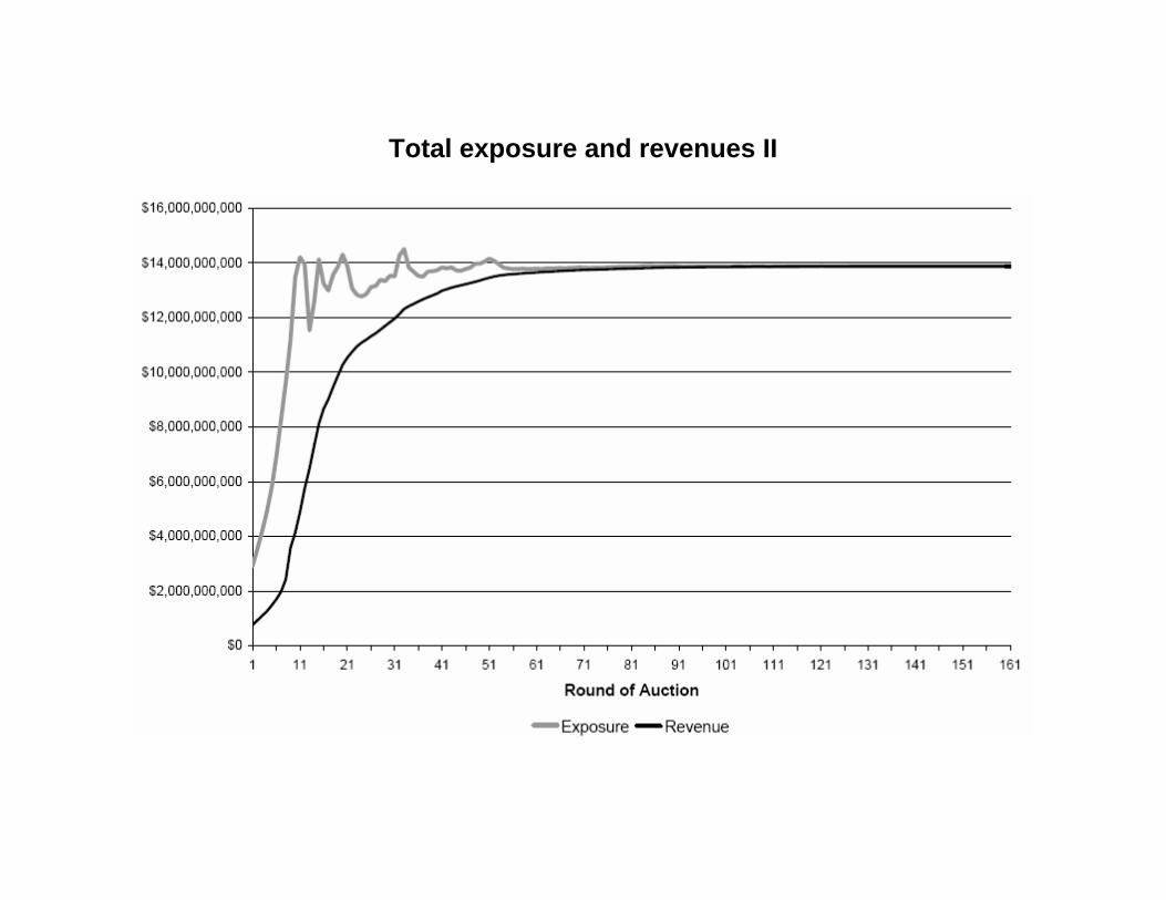
Total exposure and revenues II

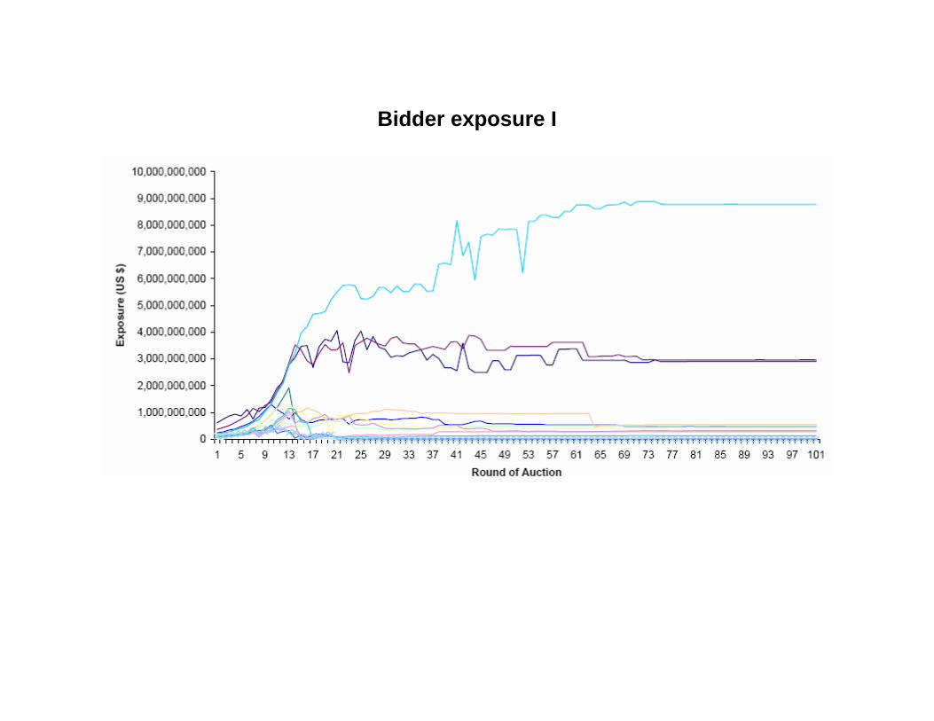
Bidder exposure I

Bidder exposure II

Purchases in the auction FCC Auction 66, Aug-Sep 2006

Performance of the five bidders spending over $1 billion

Bidder Total winning bids (billions) Price per MHz-Pop

SpectrumCo $2.4 $0.451

Cingular $1.3 $0.548

T-Mobile $4.2 $0.630

Verizon wireless $2.8 $0.731

MetroPCS $1.4 $0.963

Bargaining

The strategic approach (Rubinstein, 1982)

— Two players i = 1, 2 bargain over a “pie” of size 1.

— An agreement is a pair (x1, x2) where xi is player i’s share of the pie.

— The set of possible agreements is x1 + x2 = 1 where for any twopossible agreements x and y

x %i y if and only if xi ≥ yi

The bargaining procedure

— The players can take actions only at times in an (infinite) set of dates.

— In each period t player i, proposes an agreement (x1, x2) and playerj 6= i either accepts (Y ) or rejects (N).

— If (x1, x2) is accepted (Y ) then the bargaining ends and (x1, x2) isimplemented. If it is rejected (N) then the play passes to period t+1in which j proposes an agreement (alternating offers).

Preferences

The preferences over outcomes alone may not be sufficient to determine asolution. Time preferences (toward agreements at different points in time)are the driving force of the model:

— - Disagreement is the worst outcome.

- The pie is desirable and time is valuable.

- Increasing loss to delay.

Under this assumptions, the preferences of player i are represented by

δtiui(xi)

for any 0 < δi < 1 and ui is increasing and concave function

Any two-player bargaining game of alternating offers in which players’ pref-erences satisfy the assumptions above has a unique (!) subgame perfectequilibrium.

=⇒ Player 1 (moves first) always proposes

(x∗1, x∗2) = (

1− δ21− δ1δ2

,δ2(1− δ1)

1− δ1δ2),

and accepts an offer (y1, y2) of player 2 if and only if y1 ≥ y∗1.

=⇒ Player 2 always proposes

(y∗1, y∗2) = (

δ1(1− δ2)

1− δ1δ2,1− δ11− δ1δ2

).

and accepts an offer (x1;x2) of player 1 if and only if x2 ≥ x∗2.

The unique outcome is that player 1 proposes (x∗1, x∗2) at the first period

and player 2 accepts (no delay!).

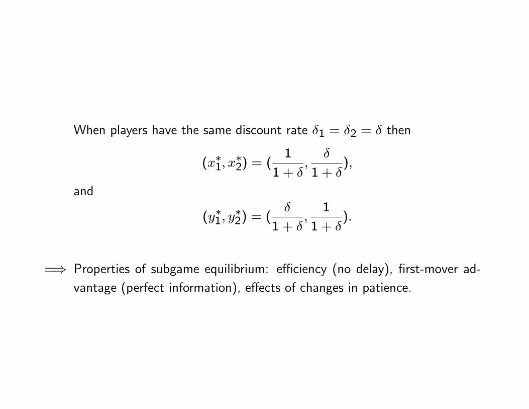
When players have the same discount rate δ1 = δ2 = δ then

(x∗1, x∗2) = (

1

1 + δ,

δ

1 + δ),

and

(y∗1, y∗2) = (

δ

1 + δ,1

1 + δ).

=⇒ Properties of subgame equilibrium: efficiency (no delay), first-mover ad-vantage (perfect information), effects of changes in patience.

The axiomatic approach (Nash, 1950)

Nash’s (1950) work is the starting point for formal bargaining theory.

— Bargaining problem: a set of utility pairs (s1; s2) that can be derivedfrom possible agreements, and a pair of utilities (d1, d2) which is des-ignated to be a disagreement point.

— Bargaining solution: a function that assigns a unique outcome to everybargaining problem.

Let S be the set of all utility pairs (s1; s2). hS, di is the primitive of Nash’sbargaining problem.

Nash’s axioms

One states as axioms several properties that it would seem natural forthe solution to have and then one discovers that the axioms actuallydetermine the solution uniquely — Nash 1953 —

[1] Invariance to equivalent utility representations (INV)

If­S0, d0

®is obtained from hS, di by “monotonic” transformations then­

S0, d0®and hS, di represent the same situation.

INV requires that the utility outcome of the bargaining problem co-varywith representation of preferences. The physical outcome predicted by thebargaining solution is the same for

­S0, d0

®and hS, di.

[2] Symmetry (SYM)

A bargaining problem hS, di is symmetric if

d1 = d2

and

(s1, s2) is in S if and only if (s2, s1) is in S.

If the bargaining problem hS, di is symmetric then the bargaining solutionmust assign the same utility.

Nash does not describe differences between the players. All asymmetries(in the bargaining abilities) must be captured by hS, di.

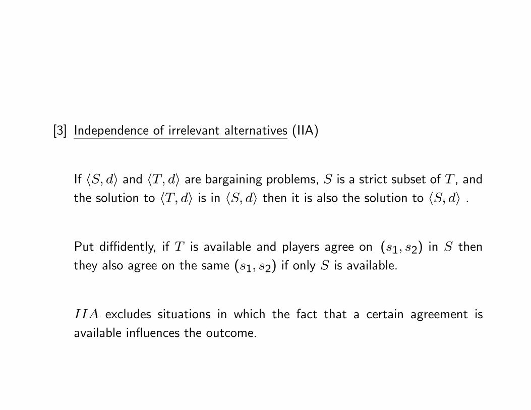
[3] Independence of irrelevant alternatives (IIA)

If hS, di and hT, di are bargaining problems, S is a strict subset of T , andthe solution to hT, di is in hS, di then it is also the solution to hS, di .

Put diffidently, if T is available and players agree on (s1, s2) in S thenthey also agree on the same (s1, s2) if only S is available.

IIA excludes situations in which the fact that a certain agreement isavailable influences the outcome.

Pareto efficiency (PAR)

If hS, di is a bargaining problem where (s1; s2) and (t1, t2) are in S andti > si for i = 1, 2 then the solution is not (s1, s2).

Players never agree on an outcome (s1, s2) when there is an outcome(t1, t2) in which both are better off.

After agreeing on the outcome (s1, s2), players can always “renegotiate”and agree on (t1, t2).

Nash’s solution

There is precisely one bargaining solution, satisfying SYM, PAR, INV andIIA.

The unique bargaining solution is the utility pair that maximizes the prod-uct of the players’ utilities

argmax(s1,s2)

s1s2

=⇒ Application: wage bargaining.