Two-Stage Stochastic and Deterministic Optimization

Tim Rzesnitzek, ∗

Dr. Heiner Mullerschon, †

Dr. Frank C. Gunther,∗

Michal Wozniak∗

Abstract

The purpose of this paper is to explore some interesting aspects of stochastic opti-mization and to propose a two-stage optimization process for highly nonlinear automotivecrash problems.

In the first stage of this process, a preliminary stochastic optimization is conductedwith a large number of design variables. The stochastic optimization serves the dualpurpose of obtaining a (nearly) optimal solution, which need not be close to the initialdesign, and of identifying a small set of design variables relevant to the optimizationproblem.

In the second stage, a deterministic optimization using only the set of relevant designvariables is conducted. The result of the preceding stochastic optimization is used as thestarting point for the deterministic optimization.

This procedure is demonstrated with a van-component model (previously introducedin [1]) used for crash calculations. LS-OPT [4] is used due to its ability to perform bothstochastic (Latin Hypercube) and deterministic optimization.

1 Stage I: Stochastic Optimization

Stochastic optimization is often performed using the Monte Carlo method, where each designvariable is individually constrained to lie within a user-specified upper and lower bound. Theinput values for these design variables are then determined randomly within their respectivebounds.

The Latin Hypercube method provided by LS-OPT is also a random experimental designprocess. Figure 1 illustrates the algorithm used for generating random values for a smallset of design variables (in this case, t1 through t4). The range of each design variable issubdivided into n equal intervals, where n is the number of experiments (in this case, thenumber of experiments is 5). A set of input variables is then determined for each experimentby randomly selecting one of the n sub-divisions for each variable. Each sub-division may beused within only one single experiment, thus ensuring that the entire design space is covered.

The distribution of design points for the Monte Carlo and Latin Hypercube algorithmscan be influenced by adding additional constraints based on response functions. This requiresa response function that depends linearly on the design variables. The responses of a new

∗DaimlerChrysler, Commercial Vehicles Analysis†DYNAmore GmbH

1

design space

- experiments

t1

t2

t3

t4

1 2 3 4 5

desi

gn v

aria

bles

Number of Experiments

Figure 1: Latin Hypercube algorithm of LS-OPT

design can then be estimated by using the initial values of the design variables together withthe corresponding initial responses.

For the optimization of a vehicle body, the mass of sheet metal parts linearly depends onsheet thickness, provided that the geometry remains unchanged. If the sheet thickness is adesign variable, the mass for a new value of the sheet thickness can be estimated by multiplyingthe new sheet thickness by the ratio of initial sheet thickness to initial mass. Hence the totalmass of all parts involved in an optimization can be estimated directly after the input valuesfor an experiment are generated and can thus be used as a variable to define a constraint.

There are several different ways for enforcing the upper and lower bounds for a constraintvariable:

1. In LS-OPT, a large number of initial design points is created. All points within thisinitial set exceeding the constraint are then shifted until they lie on the bound thathas been exceeded. This is achieved, for example, by varying the sheet thicknessessappropriately. Depending on the number of points created for the initial set, a largenumber of design points may lie on the bounds of the constraint. Thus, in the secondstage, the final set of design points is extracted from the initial set by the help of theD-optimality criterion [4].

The D-optimality criterion can be used with either a linear or quadratic approximation.The particular choice depends upon the equation applied to estimate the constraintvariable from the design variables. If, for example, mass is defined as a constraint variableand the sheet thickness of each sheet metal part are the design variables, then linearapproximation has to be used, since mass is linearly dependent from sheet thickness.

2. For the construction of a Monte Carlo design, experiments outside of the constraint arefiltered out when the set of design points is created. The generation of random values for

2

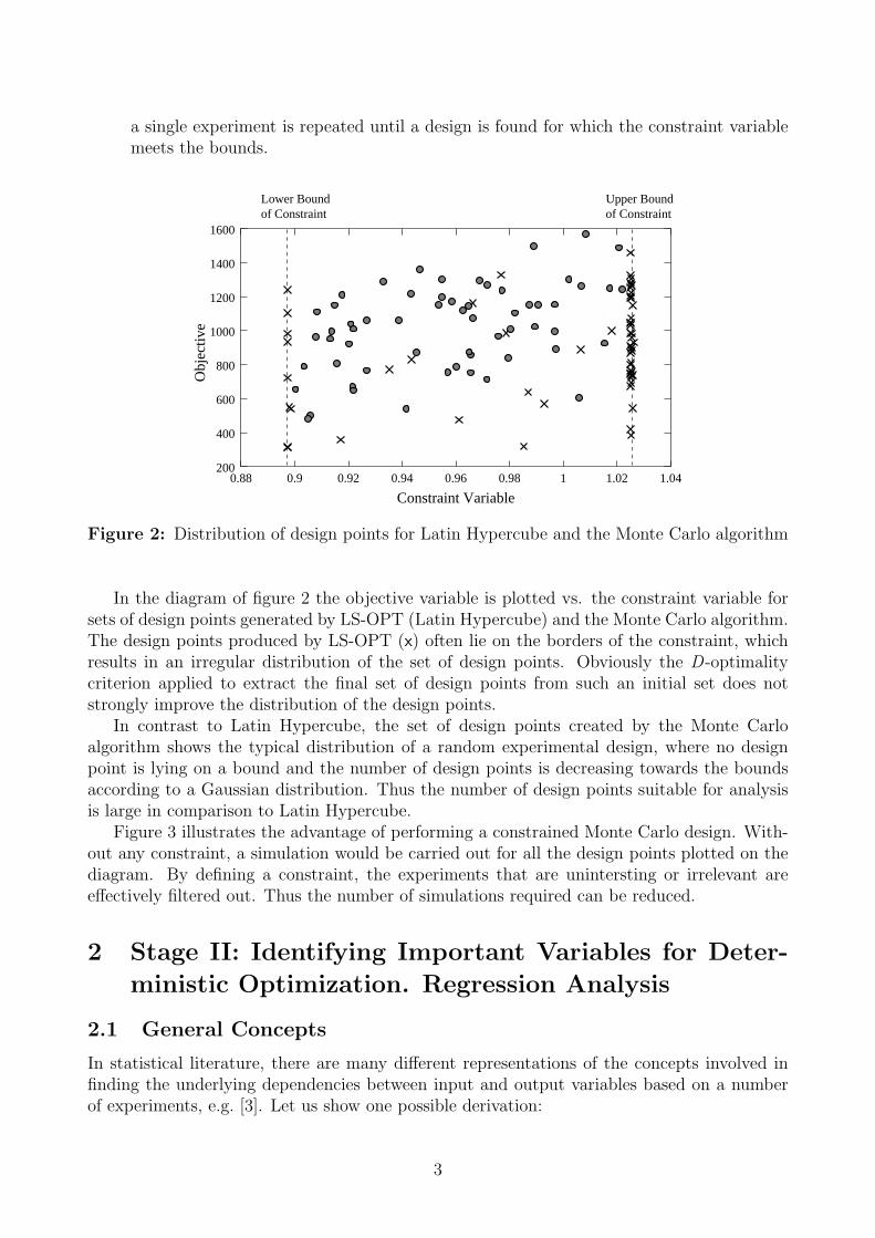
a single experiment is repeated until a design is found for which the constraint variablemeets the bounds.

Lower Boundof Constraint

Upper Boundof Constraint

1200

1400

1600

0.88 0.9 0.92 0.94 0.96

1000

0.98200

1 1.02 1.04

Obj

ectiv

e

Constraint Variable

800

600

400

Figure 2: Distribution of design points for Latin Hypercube and the Monte Carlo algorithm

In the diagram of figure 2 the objective variable is plotted vs. the constraint variable forsets of design points generated by LS-OPT (Latin Hypercube) and the Monte Carlo algorithm.The design points produced by LS-OPT (x) often lie on the borders of the constraint, whichresults in an irregular distribution of the set of design points. Obviously the D-optimalitycriterion applied to extract the final set of design points from such an initial set does notstrongly improve the distribution of the design points.

In contrast to Latin Hypercube, the set of design points created by the Monte Carloalgorithm shows the typical distribution of a random experimental design, where no designpoint is lying on a bound and the number of design points is decreasing towards the boundsaccording to a Gaussian distribution. Thus the number of design points suitable for analysisis large in comparison to Latin Hypercube.

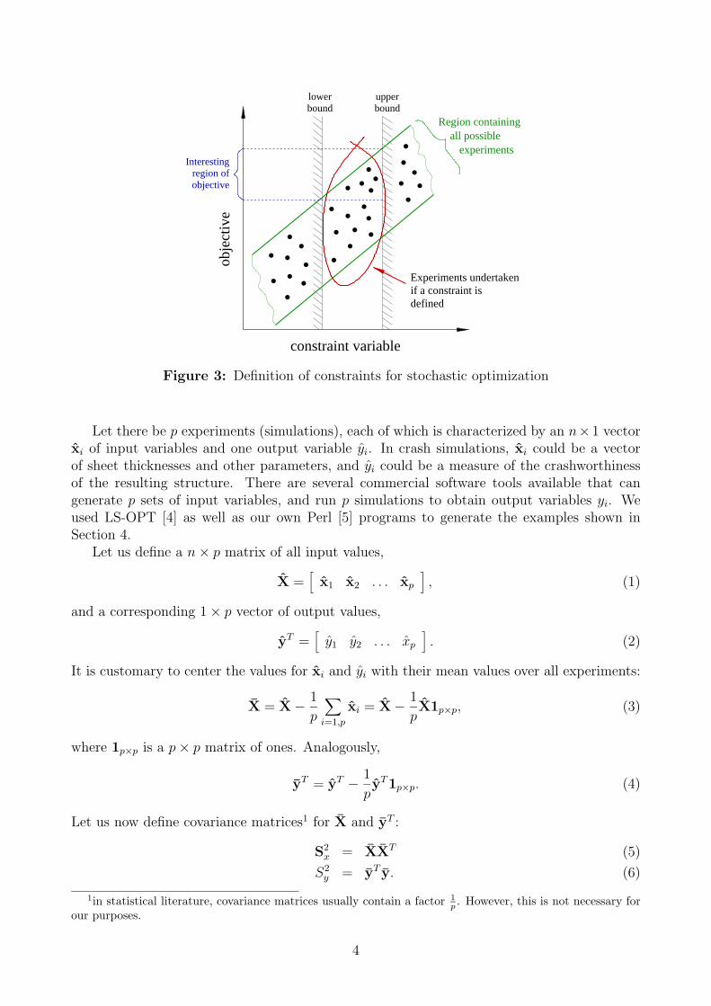
Figure 3 illustrates the advantage of performing a constrained Monte Carlo design. With-out any constraint, a simulation would be carried out for all the design points plotted on thediagram. By defining a constraint, the experiments that are unintersting or irrelevant areeffectively filtered out. Thus the number of simulations required can be reduced.

2 Stage II: Identifying Important Variables for Deter-

ministic Optimization. Regression Analysis

2.1 General Concepts

In statistical literature, there are many different representations of the concepts involved infinding the underlying dependencies between input and output variables based on a numberof experiments, e.g. [3]. Let us show one possible derivation:

3

constraint variable

upperbound

lowerbound

if a constraint isdefined

Experiments undertaken

Interestingregion ofobjective

Region containingall possible

experiments

obje

ctiv

e

Figure 3: Definition of constraints for stochastic optimization

Let there be p experiments (simulations), each of which is characterized by an n×1 vectorxi of input variables and one output variable yi. In crash simulations, xi could be a vectorof sheet thicknesses and other parameters, and yi could be a measure of the crashworthinessof the resulting structure. There are several commercial software tools available that cangenerate p sets of input variables, and run p simulations to obtain output variables yi. Weused LS-OPT [4] as well as our own Perl [5] programs to generate the examples shown inSection 4.

Let us define a n× p matrix of all input values,

X =[

x1 x2 . . . xp], (1)

and a corresponding 1× p vector of output values,

yT =[y1 y2 . . . xp

]. (2)

It is customary to center the values for xi and yi with their mean values over all experiments:

X = X− 1

p

∑i=1,p

xi = X− 1

pX1p×p, (3)

where 1p×p is a p× p matrix of ones. Analogously,

yT = yT − 1

pyT1p×p. (4)

Let us now define covariance matrices1 for X and yT :

S2x = XXT (5)

S2y = yT y. (6)

1in statistical literature, covariance matrices usually contain a factor 1p . However, this is not necessary for

our purposes.

4

It is easily established that S2x is positive semidefinite. In order to obtain the standard devia-

tion2 Sx withS2x = SxSx, (7)

we can perform an eigenvalue decomposition3 of S2x and take the square roots of the eigenvalues,

viz.

S2x = TTdiag {λi}T (8)

Sx = TTdiag{√

λi

}T (9)

λi ≥ 0 due to positive semidefiniteness. (10)

Of course,

Sy =√S2y (11)

is computed trivially.Let us now introduce the transformed variables

X = S−1x X (12)

yT = S−1y yT , (13)

assuming Sx is invertible and Sy 6= 0. These variables are normalized in the sense that

XXT = S−1x XXTS−1

x = S−1x S2

xS−1x = I (14)

yTy = S−1y yT yS−1

y = S−1y S2

yS−1y = 1. (15)

Our goal is to find a linear approximation with a n× 1 vector w such that the residual

r = y −XTw (16)

is minimized. Minimizing the quadratic norm of r is equivalent to minimizing rT r, hence thename Least Squares Approximation.

With the orthogonality conditions 14 and 15, we obtain

rT r =(yT −wTX

) (y −XTw

)(17)

= yTy − yTXTw −wTXy + wTXXTw (18)

= 1− 2wTXy + wTw (19)

In index notation, this becomes

riri = 1− 2wiXijyj + wiwi, (20)

where summation over double indices is implied.The minimum of equation 20 can be found by taking the derivative with respect to w and

setting it to zero. In index notation:

∂ (riri)

∂wk= −2δikXijyj + δikwi + wiδik (21)

= −2Xkjyj + 2wk = 2 (wk −Xkjyj) . (22)

2Give or take a factor 1√p .

3This process is significantly simplified if the input variables x are completely independent of each other.In such a case, the covariance matrix becomes diagonal: S2

x = diag {λi} and T = I, hence Sx = diag{√

λi}

5

The Kronecker delta δij is defined as

δij =

{1 if i = j0 otherwise.

(23)

Back in matrix notation, we find that

w = Xy. (24)

Our linear approximation becomes

y = wTx = yTXTx. (25)

This gives rise to interpreting the elements of w as the significance of each normalizedinput variable in the vector

x = S−1x x (26)

for the result of the simulation. Generally, the elements of x are a linear combination of theelements of x.

In terms of centered variables 3 and 4 we obtain

y = yT XT(XXT

)−1

︸ ︷︷ ︸w

x. (27)

The weight vector w contains the non-normalized regression coefficients. Hence, its valuescannot be compared to each other directly.

2.2 Variable Screening in LS-OPT (ANOVA)

LS-OPT provides the capability of performing a significance test for each variable in order toremove those coefficients or variables which have a small contribution to the design model [4].For each response, the variance of each variable with respect to that response is tracked andtested for significance using the partial F-test [2]. The importance of a variable is penalizedby both a small absolute coefficient value (weight) computed from the regression, as well as bya large uncertainty in the value of the coefficient pertaining to the variable. A 90% confidencelevel is used to quantify the uncertainty and the variables are ranked based on this level.The 100(1−α)% confidence interval for the regression coefficients bj, j = 1, ..., n is determinedby

bj −∆bj

2≤ βj ≤ bj +

∆bj2

(28)

where

∆bj = 2 tα/2,p−(n+1)

√σ2Cjj (29)

and σ2 is an unbiased estimator of the variance σ2 given by

σ2 =ε2

p− (n+ 1)=

Σpi=1(yi − yi)2

p− (n+ 1)(30)

Cjj is the diagonal element of (XT X)−1 corresponding to bj and tα/2,p−(n+1) is the t orStudent’s Distribution. ε is the error between the response yi and the estimated response yi

6

bj

∆ b0

90%

j

from linear regression

Figure 4: Confidence interval for the regression coefficient for variable j

evaluated by linear regression. 100(1 − α)% therefore represents the level of confidence thatbj will lie within the computed interval, (4).

Figure 5 demonstrates graphically the criterion for the ranking of the variables. A 90%confidence level defines the lower bound and the variables are ranked according to this lowerbound. If the lower bound is less than zero, the variable is declared as insignificant.

bj

∆ bj

bj

∆ b0

j

Insignificant

Significant

Value which determines significance

0

Figure 5: Criterion for the significance of a variable

Each variable is normalized with respect to the size of the design space. Thus all variablesrange within the interval [0,1] and a reasonable comparison can be made for variables ofdifferent kinds.

3 Description of Van Component Model for Crash

The scope of the optimization is an assembly of a vehicle body for a commercial van as shownin Figure 6.

The main components of that assembly are the first cross member and the front part of thelongitudinal member of the frame. Furthermore, the absorbing box between first cross memberand longitudinal member, parts of the wheelhouse and the closing panels of the longitudinalmember are also included in the assembly.

In Figure 7, boundary conditions and part numbers of important components are illus-trated.

The assembly is connected to the bottom sheet of the vehicle body at the flanges of thefront and back closing panels. In the simulations, the assembly is fixed in y- and z-directions

7

Figure 6: Position of the assembly within the vehicle

at these flanges. The assembly is displaced in x-direction at a constant velocity and deformsat the stonewall.

For simulation purposes, only half of the frame is represented (since geometry and loadsare symmetric to the yz-plane) and the first cross member is cut off at the yz-plane. Therefore,the translation in the y-direction and the rotation about the x- and z-axis have to be fixedalong the cutting edge.

4 Application of Concepts to the Example Model

A two-stage optimization has been performed for the component model described above. Inthe first stage, two different kinds of random distributions are applied in order to generatesamples of design variables. The two methods are a Monte Carlo distribution provided by aperl programm and a Latin Hypercube design combined with D-Optimal strategy provided byLS-OPT. The two approaches are compared to each other.

In the second stage, a deterministic optimization using the successive response surfacemethodology of LS-OPT is performed. The start design for this is the best set of variablesresulting out of the first stage.

4.1 Description of the optimization problem

The design variables consists of the sheet thicknesses of 15 parts and an additional bead locatedon the longitiudinal member on the outer and inner side. The geometry and the location ofthe bead is identical on both sides (symmetry). The bead is defined by 5 design variables,the depth t, the x-location xmin, xmax and the z-location zmin, zmax. Preprocessing of theLS-DYNA input file for the bead is done by a Perl programm (for additional information, see[1]). In total there are 20 design variables.

The objective of the optimization is to maximize the ratio of the maximum value of theinternal energy Emax and the mass M of the considered components:

8

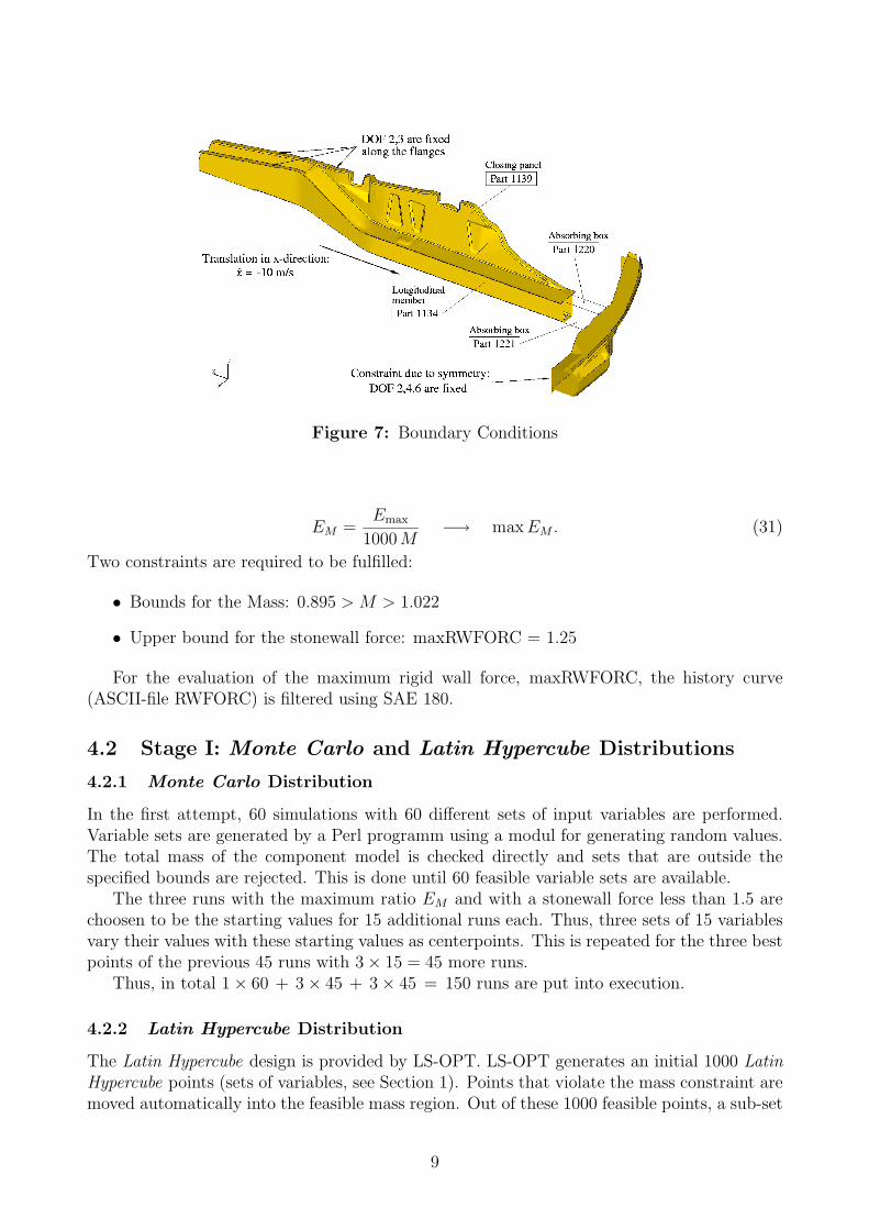
Figure 7: Boundary Conditions

EM =Emax

1000M−→ maxEM . (31)

Two constraints are required to be fulfilled:

• Bounds for the Mass: 0.895 > M > 1.022

• Upper bound for the stonewall force: maxRWFORC = 1.25

For the evaluation of the maximum rigid wall force, maxRWFORC, the history curve(ASCII-file RWFORC) is filtered using SAE 180.

4.2 Stage I: Monte Carlo and Latin Hypercube Distributions

4.2.1 Monte Carlo Distribution

In the first attempt, 60 simulations with 60 different sets of input variables are performed.Variable sets are generated by a Perl programm using a modul for generating random values.The total mass of the component model is checked directly and sets that are outside thespecified bounds are rejected. This is done until 60 feasible variable sets are available.

The three runs with the maximum ratio EM and with a stonewall force less than 1.5 arechoosen to be the starting values for 15 additional runs each. Thus, three sets of 15 variablesvary their values with these starting values as centerpoints. This is repeated for the three bestpoints of the previous 45 runs with 3× 15 = 45 more runs.

Thus, in total 1× 60 + 3× 45 + 3× 45 = 150 runs are put into execution.

4.2.2 Latin Hypercube Distribution

The Latin Hypercube design is provided by LS-OPT. LS-OPT generates an initial 1000 LatinHypercube points (sets of variables, see Section 1). Points that violate the mass constraint aremoved automatically into the feasible mass region. Out of these 1000 feasible points, a sub-set

9

deformed model

undeformed model

Figure 8: Simulation model - initial and deformed configuration

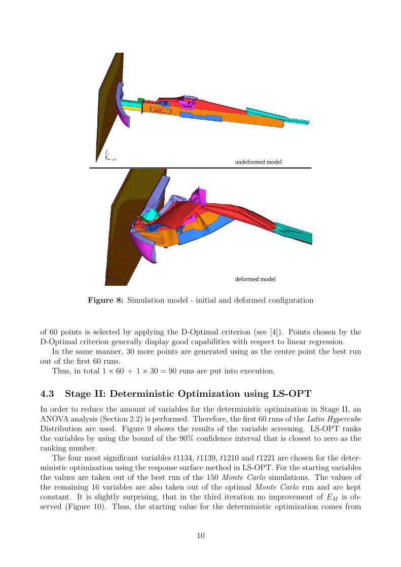
of 60 points is selected by applying the D-Optimal criterion (see [4]). Points chosen by theD-Optimal criterion generally display good capabilities with respect to linear regression.

In the same manner, 30 more points are generated using as the centre point the best runout of the first 60 runs.

Thus, in total 1× 60 + 1× 30 = 90 runs are put into execution.

4.3 Stage II: Deterministic Optimization using LS-OPT

In order to reduce the amount of variables for the deterministic optimization in Stage II, anANOVA analysis (Section 2.2) is performed. Therefore, the first 60 runs of the Latin HypercubeDistribution are used. Figure 9 shows the results of the variable screening. LS-OPT ranksthe variables by using the bound of the 90% confidence interval that is closest to zero as theranking number.

The four most significant variables t1134, t1139, t1210 and t1221 are chosen for the deter-ministic optimization using the response surface method in LS-OPT. For the starting variablesthe values are taken out of the best run of the 150 Monte Carlo simulations. The values ofthe remaining 16 variables are also taken out of the optimal Monte Carlo run and are keptconstant. It is slightly surprising, that in the third iteration no improvement of EM is ob-served (Figure 10). Thus, the starting value for the deterministic optimization comes from

10

Approximating Response ’E_M’ using 60 points−−−−−−−−−−−−−−−−−−−−−−−−−−−−−−−−−−−−−−−−−−−−−−

Linear Function Approximation:−−−−−−−−−−−−−−−−−−−−−−−−−−−−−−Mean response value = 0.8890RMS error = 0.2238 (12.33%)Maximum Residual = 0.4611 (25.40%)Average Error = 0.1824 (10.05%)Square Root PRESS Residual = 0.3687 (20.31%)Variance = 0.0751R^2 = 0.8524R^2 (adjusted) = 0.8524R^2 (prediction) = 0.5995

Individual regression coefficients: confidence intervals−−−−−−−−−−−−−−−−−−−−−−−−−−−−−−−−−−−−−−−−−−−−−−−−−−−−−−−−

| Coeff. | Confidence Int.(90%)| Confidence Int.(95%) |% Confidence Coeff| |−−−−−−−−−−−−−−−−−−−−−|−−−−−−−−−−−−−−−−−−−−−−| not | Value | Lower | Upper | Lower | Upper | zero −−−−−|−−−−−−−−−−|−−−−−−−−−−|−−−−−−−−−−|−−−−−−−−−−|−−−−−−−−−−−|−−−−−− t1134| 1.58| 1.255| 1.906| 1.19| 1.971| 100 t1139| 1.015| 0.7089| 1.321| 0.6476| 1.382| 100 t1140| −0.6216| −0.9263| −0.3169| −0.9874| −0.2559| 100 t1144| −0.2674| −0.6063| 0.07145| −0.6743| 0.1394| 80 t1210| −1.055| −1.416| −0.6931| −1.489| −0.6206| 100 t1211| −0.4619| −0.8002| −0.1236| −0.868| −0.05573| 97 t1220| −0.5574| −0.8209| −0.294| −0.8737| −0.2411| 100 t1221| −0.9985| −1.337| −0.6604| −1.404| −0.5926| 100 t1222| 0.3766| 0.01415| 0.739| −0.05852| 0.8117| 91 t1223| −0.2613| −0.6392| 0.1165| −0.7149| 0.1923| 74 t1224| −0.1445| −0.4433| 0.1543| −0.5032| 0.2142| 57 t1410| −0.0268| −0.3932| 0.3396| −0.4666| 0.413| 10 t1411| −0.05109| −0.3883| 0.2861| −0.4559| 0.3537| 20 t1412| −0.544| −0.8206| −0.2674| −0.876| −0.212| 100 t1413| −0.3308| −0.7064| 0.04484| −0.7818| 0.1202| 85 xmin | 0.3381| −0.06837| 0.7446| −0.1499| 0.8261| 83 xmax | −0.3318| −0.5868| −0.07684| −0.638| −0.02572| 96 zmin | 0.2477| −0.02525| 0.5206| −0.07996| 0.5753| 86 zmax | −0.1905| −0.5596| 0.1786| −0.6336| 0.2526| 60 t | 0.1564| −0.1283| 0.4412| −0.1854| 0.4983| 63 −−−−−|−−−−−−−−−−|−−−−−−−−−−|−−−−−−−−−−|−−−−−−−−−−|−−−−−−−−−−−|−−−−−−

Ranking of terms based on bound of confidence interval−−−−−−−−−−−−−−−−−−−−−−−−−−−−−−−−−−−−−−−−−−−−−−−−−−−−−−

Coeff|Absolute Value (90%)|10−Scale −−−−−|−−−−−−−−−−−−−−−−−−−−|−−−−−−−− t1134| 1.255 | 10.0 t1139| 0.7089 | 5.6 t1210| 0.6931 | 5.5 t1221| 0.6604 | 5.3 t1140| 0.3169 | 2.5 t1220| 0.294 | 2.3 t1412| 0.2674 | 2.1 t1211| 0.1236 | 1.0 xmax | 0.07684 | 0.6 t1222| 0.01415 | 0.1 zmin | Insignificant | 0.0 t1413| Insignificant | 0.0 xmin | Insignificant | 0.0 t1144| Insignificant | 0.0 t1223| Insignificant | 0.0 t | Insignificant | 0.0 t1224| Insignificant | 0.0 zmax | Insignificant | 0.0 t1411| Insignificant | 0.0 t1410| Insignificant | 0.0 −−−−−|−−−−−−−−−−−−−−−−−−−−|−−−−−−−−

Variables kept constant in Stage II

Selected Variables for Stage II

Figure 9: Output of LS-OPT for variable screening with respect to the response EM

the sample distribution of the second iteration. Within the Latin Hypercube samples, the bestresult with respect to the maximum Energy-Mass ratio EM is significantly worse than thebest result for the Monte Carlo samples (compare Figure 10). This is probably due to themovement of the variables in order to fulfill the mass constraints. This leads to a degeneratedsample distribution with an accumulation of samples at the lower and upper bound of themass constraints (Figure 2).Figure 10 shows the results of the Monte Carlo and the Latin Hypercube simulations of StageI and the result of an optimum run found by LS-OPT using the response surface methodologyin Stage II. A significant additional improvement of the response EM by the deterministicapproach is observed.

11

5 Conclusions

The present paper shows the proceeding of a two-stage optimization, where in the first stagea stochastic approach is considered and in the second stage, starting from the best result ofthe first stage, a deterministic optimization using the Response Surface Method in LS-OPTis performed.The variation of the design variables (sheet thicknesses) is restricted by a mass constraint.This is done in order to achieve only samples whose mass lies within a desired range. Thisensures that needless simulations are avoided.On the basis of a set of Latin Hypercube simulations, a variable screening using the ANOVA(ANalysis Of VAriance) feature in LS-OPT is performed. With this tool, those variablesdetected as insignificant are removed for the second stage of the optimization process.

The starting variables for the deterministic optimization in the second stage are takenout of the best run of the Monte Carlo simulations. A significant additional improvement ofthe Energy/Mass ratio by the deterministic approach is observed. In total, an improvementof 32.78 % from the initial configuration (1.205) to the optimum result of LS-OPT (1.60) isachieved (Figure 10).The combination of stochastic and deterministic optimization has shown to be a reasonablemethod for obtaining sensible input values for a deterministic optimization. Furthermore, itcan be expected that in many cases, the convergence of the deterministic algorithm to localextremal values with respect to the objective may be avoided.

References

[1] F. Gunther and T. Rzesnitzek. Crashworthiness optimization of van components withls-opt. In Proceedings of 19th CAD-FEM Users’ Meeting, 2001.

[2] R. Myers and M. D.C. Response Surface Methodology. Wiley New York, 1995.

[3] H. Rinne. Statistische Analyse multivariater Daten: Einfuhrung. R. Oldenbourg VerlagMunchen Wien, 2000.

[4] N. Stander and K. Craig. LS-OPT User’s Manual: Design Optimization Software for theEngineering Analyst. Livermore Software Technology Corporation, 2002.

[5] L. Wall, T. Christiansen, and J. Orwant. Programming Perl. O’Reilly & Associates, 3rdedition, 2000.

12

Best Result M.Carlo2

Best Result M.Carlo1

Best Result M.Carlo3Best Result LatinHyperCube

Result Optimum

RWFORC=1.25 (constraint)

RWFORC=1.25 (constraint)

Result Initial Configuration

Result Optimum

LatinHyperCube/D−Optimal

RSM LS−OPT

MonteCarlo Iter1MonteCarlo Iter2MonteCarlo Iter3Result Initial ConfigurationResult Optimum RSM LS−OPT

RSM LS−OPT

1.1

1.15

1.2

1.25

1.3

1.35

1.4

1.25 1.3 1.35 1.4 1.45 1.5 1.55 1.6

0.4

0.6

0.8

1

1.2

1.4

1.6

1.8

0.6 0.8 1 1.2 1.4 1.6E_M

RW

FOR

CR

WFO

RC

Figure 10: Response EM vs. the corresponding rigid wall force RWFORC for Latin Hypercubeand Monte Carlo Samples and for the final optimum found by the Response Surface Method(RSM) in Stage II

13