two stable methods with numerical experiments for solving the backward heat equation
DESCRIPTION
Two Stable Methods With Numerical Experiments for Solving the Backward Heat EquationTRANSCRIPT
Applied Numerical Mathematics 61 (2011) 266–284
Contents lists available at ScienceDirect
Applied Numerical Mathematics
www.elsevier.com/locate/apnum
Two stable methods with numerical experiments for solving thebackward heat equation
Fabien Ternat a, Oscar Orellana b, Prabir Daripa c,∗a Institut de Recherche sur les Phénomènes Hors-Équilibre, IRPHE, Marseille, Franceb Departamento de matemáticas, Universidad Técnica Santa María de Valparaíso, UTFSM, Chilec Department of Mathematics, Texas A&M University, College Station, TX, United States
a r t i c l e i n f o a b s t r a c t
Article history:Received 3 December 2009Received in revised form 17 July 2010Accepted 9 September 2010Available online 14 October 2010
Keywords:Backward heat equationIll-posed problemNumerical methodsCrank–Nicolson methodEuler schemeDispersion relationFilteringRegularization
This paper presents results of some numerical experiments on the backward heatequation. Two quasi-reversibility techniques, explicit filtering and structural perturbation,to regularize the ill-posed backward heat equation have been used. In each of thesetechniques, two numerical methods, namely Euler and Crank–Nicolson (CN), have beenused to advance the solution in time.Crank–Nicolson method is very counter-intuitive for solving the backward heat equationbecause the dispersion relation of the scheme for the backward heat equation has asingularity (unbounded growth) for a particular wave whose finite wave number dependson the numerical parameters. In comparison, the Euler method shows only catastrophicgrowth of relatively much shorter waves. Strikingly we find that use of smart filteringtechniques with the CN method can give as good a result, if not better, as with the Eulermethod which is discussed in the main text. Performance of these regularization methodsusing these numerical schemes have been exemplified.
© 2010 IMACS. Published by Elsevier B.V. All rights reserved.
1. Introduction
The problem of heat conduction through a conducting medium occupying a space Ω subject to no heat flux across theboundary of the region is formulated as follows:
⎧⎨⎩
ut − νuxx = 0, x ∈ Ω, t > 0,
ux|∂Ω = 0, t > 0,
u(x,0) = u0(x), x ∈ Ω.
(1)
Here u(x, t) is the temperature and u0(x) is the initial temperature distribution. This problem is known to be well-posedin the sense of Hadamard, i.e. existence, uniqueness and continuous dependence of the solution on the boundary dataare well-established for this problem. The above problem is usually referred as a forward problem in the context of heatequation.
The backward problem related to the heat equation refers to the problem of finding the initial temperature distributionof the forward problem from a knowledge of the final temperature distribution v0(x) at time T :
* Corresponding author.E-mail address: [email protected] (P. Daripa).
0168-9274/$30.00 © 2010 IMACS. Published by Elsevier B.V. All rights reserved.doi:10.1016/j.apnum.2010.09.006
F. Ternat et al. / Applied Numerical Mathematics 61 (2011) 266–284 267
⎧⎨⎩
ut − νuxx = 0, x ∈ Ω, t ∈ [0, T ],ux|∂Ω = 0,
u(x, T ) = v0(x), x ∈ Ω.
(2)
The change of variable t → T − t leads to the following formulation of this backward problem where v(x, t) = u(x, T − t):⎧⎨⎩
vt + νvxx = 0, x ∈ Ω, t ∈ [0, T ],vx|∂Ω = 0,
v(x,0) = v0(x), x ∈ Ω.
(3)
This backward problem is ill-posed on all three counts: existence, uniqueness and continuous dependence of solution onarbitrary initial data (see Nash [19], John [11], Miranker [17] and Hollig [9]), though this problem is well-posed for initialdata whose Fourier spectrum has compact support (see Miranker [17]). However, in practice, an initial data cannot in generalbe guaranteed to have a compact support in Fourier space. When an initial data has a compact support in Fourier space, itloses this compactness in practice for a variety of reasons such as measurement error, noise in the measured data, round-offerror in machine representations of such data, just to mention a few reasons. Integrating such equations by any numericalscheme further compounds this problem due to the effect of truncation error. Because of these reasons, even when a uniquesolution of the backward problem exists for some particular initial data, computing such a solution in some stable way hasbeen a challenge for a long time (see Douglas and Gallie [6], John [11], Pucci [20]).
A constructive approach to circumvent this computational challenge is to analyze first the dispersion relation. The dis-persion relation associated with the backward heat equation is ω = k2, i.e. a mode with wave number k grows quadratically.This kind of catastrophic growth of short waves is also an indication that solutions (classical) of the backward problemmay not always exist for all time for arbitrary initial data. This is all too well known for the backward heat equation forwe know that any discontinuous temperature profile gets smoothed out instantaneously by forward heat equation. Anotherconsequence of this is the undesirable catastrophic growth of errors (in particular in high wave number modes) arising dueto numerical approximation of the equation (truncation error), the machine representation of the data (roundoff error) andnoise in any measured data.
In this paper, computation of solutions of this ill-posed backward heat equation is undertaken on appropriately chosenspace–time grid in conjunction with filtering and regularization techniques. We present numerical results that show thatsolutions can be computed in stable ways for times longer than earlier reported by clever choice of the grids, filters,regularization term and clever dynamic application of the chosen filters. We also present detail outline of the proceduresso that the computational results presented here can be reproduced by anyone interested in doing so. It is worth pointingout here that the filtering techniques reported earlier in the literature with other ill-posed problems (see [13,22,4,5,8]) havebeen applied here successfully to this backward heat problem.
2. Numerical schemes and results
The computational domain Ω is taken to be one dimensional, in particular Ω = [0,1]. We discretize the interval [0,1]with M subintervals �x = 1/M of equal length with grid points denoted by xm , m = 0, . . . , M . Integration in time is donein time step of �t with time interval T = N × �t and tn = n × �t , n = 0, . . . , N . The exact value of the solution at (xm, tn)
is denoted by v(xm, tn) and numerical value by vnm . Zero Neumann boundary conditions at both end points of the interval
[0,1] are approximated that results in the following third order accurate end point values of v for t > 0,
v(0, t) = 4v(�x, t) − v(2�x, t)
3+ O
((�x)3), (4)
v(1, t) = 4v(1 − �x, t) − v(1 − 2�x, t)
3+ O
((�x)3). (5)
2.1. Euler scheme
In terms of forward and backward finite difference operators D+ and D− , the finite difference equation for the backwardheat equation is
D+t vn
m
�t= −ν
D+x D−
x vnm
�x2, ∀m �= {1, M}, ∀n > 2. (6)
For numerical construction of solutions, it is useful to choose appropriate values of �x and �t so that numerical and exactdispersion relations do not deviate too much from each other over a range of participating wave numbers. Using the ansatzvn
m = ρneiξm (where ρ = eβ�t and ξ = kπ�x) in the finite difference equation (6) yields the dispersion relation,
ρ = 1 + 4νr sin2 (kπ�x/2), (7)
where r = �t/�x2. When �x → 0, we have ρ ∼ 1 + (kπ)2ν�t which gives, in the limit �t → 0, β = ln |ρ|/�t ∼ ν(kπ)2
which is same as the exact growth rate.
268 F. Ternat et al. / Applied Numerical Mathematics 61 (2011) 266–284
2.2. Crank–Nicolson scheme
The backward heat equation in this scheme is discretized as
D+t vn
m
�t= − ν
2�x2
(D+
x D−x vn+1
m + D+x D−
x vnm
). (8)
For dispersion relation, same ansatz for vnm as in the Euler scheme is inserted in the finite difference equation (8). This
yields the following dispersion relation
ρ = 1 + 2νr sin2 (ξ2 )
1 − 2νr sin2 ξ2
, (9)
where r = �t/�x2 as before. When �x → 0, we have
ρ ∼ 1 + ν(kπ)2 �t2
1 − ν(kπ)2 �t2
,
which gives, in the limit �t → 0, β = ln |ρ|/�t ∼ ν(kπ)2 which is the same as the exact dispersion relation. For r > 1/2ν ,the dispersion relation has a singularity at k = ku given by
ku = 2
π�xarcsin
(�x√2ν�t
). (10)
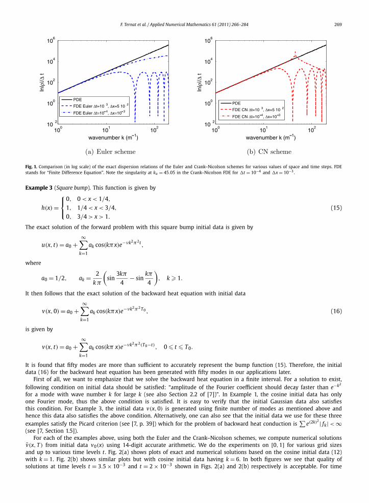
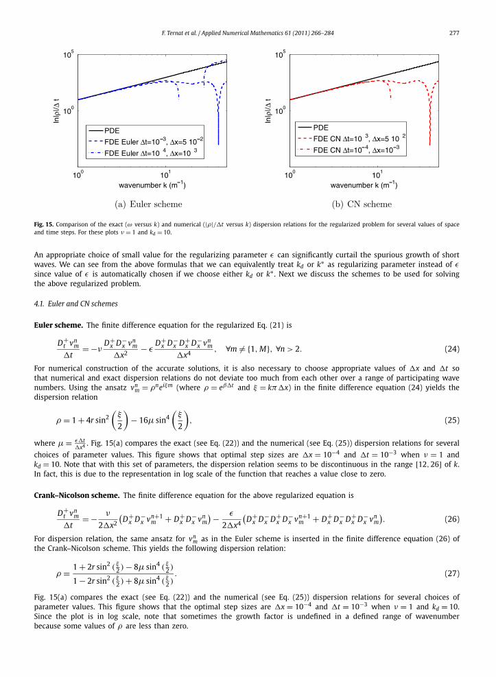
Figs. 1(a) and 1(b) compare the exact dispersion relation with the numerical ones for several values of space and time stepsrespectively for both the Euler and the CN schemes. The plots are log–log plots due to the large values of growth rates.Numerical dispersion plot for the CN scheme corresponding to �x = 10−3 and �t = 10−4 for which r > 1/2ν clearly showsthe location of the singularity at ku = 45.05. Since the singularity and high values of the growth rate are very localized neara very high wave number with rest of the dispersion curves comparing favorably with the exact one, larger time steps maystill be able to yield reasonably accurate solutions on the same grid �x as for the other dispersion curves in the figure. Wewill test below whether this is indeed true or not. For the other choices of grid values used for the CN case in the figure,r is less than 1/2 (r < 1/2ν). This figure shows that numerical dispersion curves compare favorably with the exact one upto a higher wave number for the CN scheme than for the Euler scheme. However, they all are almost same for up to a wavenumber approximately 25.
2.3. Numerical results
Numerical experiments have been performed on many problems but the results from the ones corresponding to only thefollowing problems are presented below for brevity.
Example 1 (Single cosine mode). It is easy to see that the function
ve(x, t) = cos(kπx)exp(−k2π2ν(T0 − t)
), (11)
is the solution of the backward heat equation with initial data
v0(x) = cos(kπx)exp(−k2π2νT0
). (12)
Note that vx(x, t) = 0 at x = 0,1 for all t > 0.
Example 2 (Gaussian). It is easy to check that
v(x, t) = 1√5 − 4t
exp
(− (x − 0.5)2
ν(5 − 4t)
), 0 � t � 1, (13)
is the solution of the backward heat equation with initial data
v(x,0) = 1√5
exp
(− (x − 0.5)2
5ν
). (14)
It follows that
vx(x, t) = −2(x − 0.5)
ν(5 − 4t)3/2exp
(− (x − 0.5)2
ν(5 − 4t)
), 0 � t � 1,
which is not exactly zero at the end points. It can be made close to zero by choosing a small value of ν .
F. Ternat et al. / Applied Numerical Mathematics 61 (2011) 266–284 269
Fig. 1. Comparison (in log scale) of the exact dispersion relations of the Euler and Crank–Nicolson schemes for various values of space and time steps. FDEstands for “Finite Difference Equation". Note the singularity at ku = 45.05 in the Crank–Nicolson FDE for �t = 10−4 and �x = 10−3.
Example 3 (Square bump). This function is given by
h(x) =⎧⎨⎩
0, 0 < x < 1/4,
1, 1/4 < x < 3/4,
0, 3/4 > x > 1.
(15)
The exact solution of the forward problem with this square bump initial data is given by
u(x, t) = a0 +∞∑
k=1
ak cos(kπx)e−νk2π2t,
where
a0 = 1/2, ak = 2
k π
(sin
3kπ
4− sin
kπ
4
), k � 1.
It then follows that the exact solution of the backward heat equation with initial data
v(x,0) = a0 +∞∑
k=1
ak cos(kπx)e−νk2π2 T0 , (16)
is given by
v(x, t) = a0 +∞∑
k=1
ak cos(kπ x)e−νk2π2(T0−t), 0 � t � T0.
It is found that fifty modes are more than sufficient to accurately represent the bump function (15). Therefore, the initialdata (16) for the backward heat equation has been generated with fifty modes in our applications later.
First of all, we want to emphasize that we solve the backward heat equation in a finite interval. For a solution to exist,following condition on initial data should be satisfied: “amplitude of the Fourier coefficient should decay faster than e−k2
for a mode with wave number k for large k (see also Section 2.2 of [7])”. In Example 1, the cosine initial data has onlyone Fourier mode, thus the above condition is satisfied. It is easy to verify that the initial Gaussian data also satisfiesthis condition. For Example 3, the initial data v(x,0) is generated using finite number of modes as mentioned above andhence this data also satisfies the above condition. Alternatively, one can also see that the initial data we use for these threeexamples satisfy the Picard criterion (see [7, p. 39]) which for the problem of backward heat conduction is
∑e(2k)2 | fk| < ∞
(see [7, Section 1.5]).For each of the examples above, using both the Euler and the Crank–Nicolson schemes, we compute numerical solutions
v(x, T ) from initial data v0(x) using 14-digit accurate arithmetic. We do the experiments on [0,1] for various grid sizesand up to various time levels t . Fig. 2(a) shows plots of exact and numerical solutions based on the cosine initial data (12)with k = 1. Fig. 2(b) shows similar plots but with cosine initial data having k = 6. In both figures we see that quality ofsolutions at time levels t = 3.5 × 10⁻³ and t = 2 × 10⁻³ shown in Figs. 2(a) and 2(b) respectively is acceptable. For time
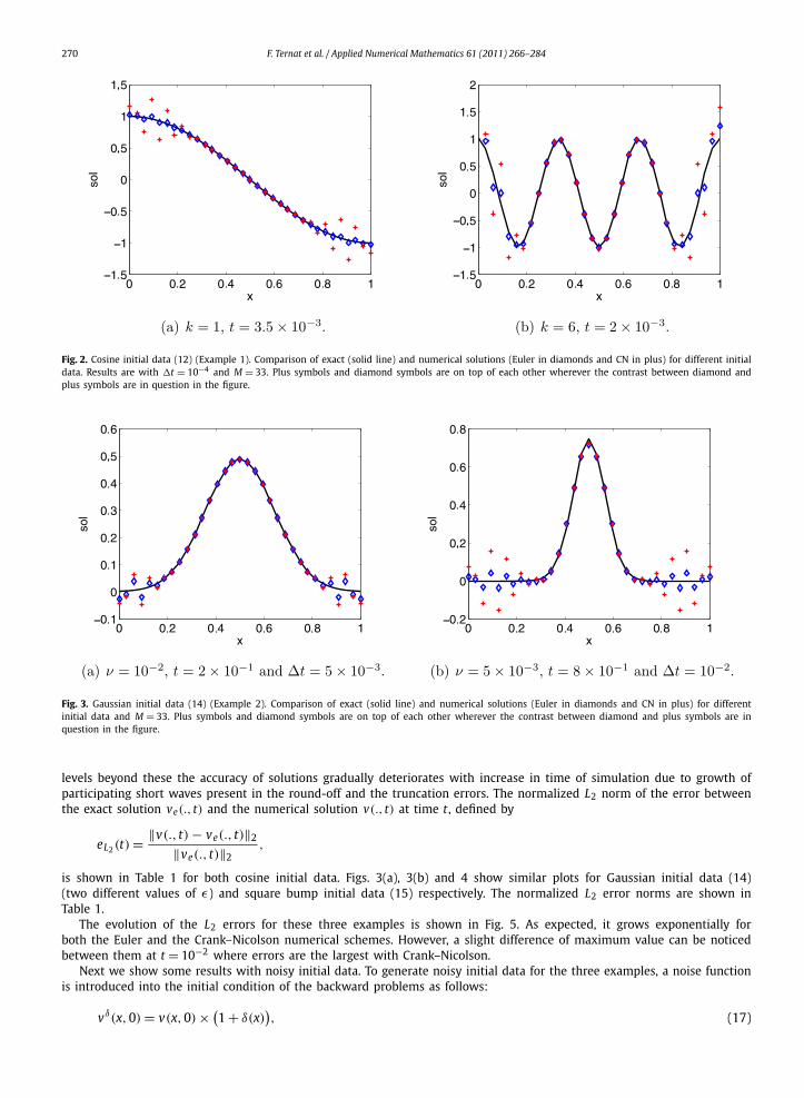
270 F. Ternat et al. / Applied Numerical Mathematics 61 (2011) 266–284
Fig. 2. Cosine initial data (12) (Example 1). Comparison of exact (solid line) and numerical solutions (Euler in diamonds and CN in plus) for different initialdata. Results are with �t = 10−4 and M = 33. Plus symbols and diamond symbols are on top of each other wherever the contrast between diamond andplus symbols are in question in the figure.
Fig. 3. Gaussian initial data (14) (Example 2). Comparison of exact (solid line) and numerical solutions (Euler in diamonds and CN in plus) for differentinitial data and M = 33. Plus symbols and diamond symbols are on top of each other wherever the contrast between diamond and plus symbols are inquestion in the figure.
levels beyond these the accuracy of solutions gradually deteriorates with increase in time of simulation due to growth ofparticipating short waves present in the round-off and the truncation errors. The normalized L2 norm of the error betweenthe exact solution ve(., t) and the numerical solution v(., t) at time t , defined by
eL2(t) = ‖v(., t) − ve(., t)‖2
‖ve(., t)‖2,
is shown in Table 1 for both cosine initial data. Figs. 3(a), 3(b) and 4 show similar plots for Gaussian initial data (14)(two different values of ε) and square bump initial data (15) respectively. The normalized L2 error norms are shown inTable 1.
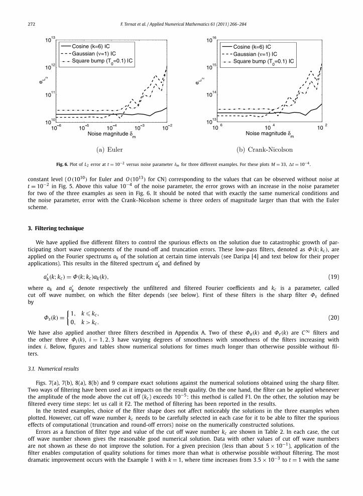
The evolution of the L2 errors for these three examples is shown in Fig. 5. As expected, it grows exponentially forboth the Euler and the Crank–Nicolson numerical schemes. However, a slight difference of maximum value can be noticedbetween them at t = 10−2 where errors are the largest with Crank–Nicolson.
Next we show some results with noisy initial data. To generate noisy initial data for the three examples, a noise functionis introduced into the initial condition of the backward problems as follows:
vδ(x,0) = v(x,0) × (1 + δ(x)
), (17)
F. Ternat et al. / Applied Numerical Mathematics 61 (2011) 266–284 271
Fig. 4. Bump square data (15) (Example 3). Comparison of exact (solid line) and numerical solutions (Euler in diamonds and CN in plus) for M = 33. Plussymbols and diamond symbols are on top of each other wherever the contrast between diamond and plus symbols are in question in the figure.
Fig. 5. Plot of L2 error versus time for three different examples without noise. For these plots M = 33, �t = 10−4.
Table 1Relative error norms without filtering.
IC �t Time Schemes eL2
Cosine Euler 2.06 × 10⁻²
k = 1 10−4 t = 3.5 × 10⁻³ CN 1.99 × 10⁻¹
Cosine Euler 1.45 × 10⁻¹
k = 6 10−4 t = 2 × 10⁻³ CN 4.5 × 10⁻¹
Gaussian Euler 5.41 × 10⁻²
ν = 10−2 5 × 10⁻³ t = 2 × 10⁻¹ CN 9.85 × 10⁻²
Gaussian Euler 8 × 10⁻²
ν = 5 × 10⁻³ 10−2 t = 8 × 10⁻¹ CN 2.88 × 10⁻¹
Example 3 Euler 4.08 × 10⁻³
T0 = 10−1 10−5 t = 3 × 10⁻³ CN 5.04 × 10⁻³
where δ(x) is the noise generated using the MatLab function “rand” multiplied by a magnitude coefficient δm:
δ(x) = δm × rand(x). (18)
For a fixed time t = 10−2, Fig. 6 shows the plots of the L2 error as a function of the noise parameter δm for both the Eulerand the Crank–Nicolson schemes. In both cases, when the noise parameter is less than about 10−4, the error remains at a
272 F. Ternat et al. / Applied Numerical Mathematics 61 (2011) 266–284
Fig. 6. Plot of L2 error at t = 10−2 versus noise parameter δm for three different examples. For these plots M = 33, �t = 10−4.
constant level (O (1010) for Euler and O (1013) for CN) corresponding to the values that can be observed without noise att = 10−2 in Fig. 5. Above this value 10−4 of the noise parameter, the error grows with an increase in the noise parameterfor two of the three examples as seen in Fig. 6. It should be noted that with exactly the same numerical conditions andthe noise parameter, error with the Crank–Nicolson scheme is three orders of magnitude larger than that with the Eulerscheme.
3. Filtering technique
We have applied five different filters to control the spurious effects on the solution due to catastrophic growth of par-ticipating short wave components of the round-off and truncation errors. These low-pass filters, denoted as Φ(k;kc), areapplied on the Fourier spectrums ak of the solution at certain time intervals (see Daripa [4] and text below for their properapplications). This results in the filtered spectrum a′
k and defined by
a′k(k;kc) = Φ(k;kc)ak(k), (19)
where ak and a′k denote respectively the unfiltered and filtered Fourier coefficients and kc is a parameter, called
cut off wave number, on which the filter depends (see below). First of these filters is the sharp filter Φs definedby
Φs(k) ={
1, k � kc,
0, k > kc .(20)
We have also applied another three filters described in Appendix A. Two of these Φa(k) and Φe(k) are C∞ filters andthe other three Φi(k), i = 1,2,3 have varying degrees of smoothness with smoothness of the filters increasing withindex i. Below, figures and tables show numerical solutions for times much longer than otherwise possible without fil-ters.
3.1. Numerical results
Figs. 7(a), 7(b), 8(a), 8(b) and 9 compare exact solutions against the numerical solutions obtained using the sharp filter.Two ways of filtering have been used as it impacts on the result quality. On the one hand, the filter can be applied wheneverthe amplitude of the mode above the cut off (kc) exceeds 10−5: this method is called F1. On the other, the solution may befiltered every time steps: let us call it F2. The method of filtering has been reported in the results.
In the tested examples, choice of the filter shape does not affect noticeably the solutions in the three examples whenplotted. However, cut off wave number kc needs to be carefully selected in each case for it to be able to filter the spuriouseffects of computational (truncation and round-off errors) noise on the numerically constructed solutions.
Errors as a function of filter type and value of the cut off wave number kc are shown in Table 2. In each case, the cutoff wave number shown gives the reasonable good numerical solution. Data with other values of cut off wave numbersare not shown as these do not improve the solution. For a given precision (less than about 5 × 10⁻¹), application of thefilter enables computation of quality solutions for times more than what is otherwise possible without filtering. The mostdramatic improvement occurs with the Example 1 with k = 1, where time increases from 3.5 × 10⁻³ to t = 1 with the same

F. Ternat et al. / Applied Numerical Mathematics 61 (2011) 266–284 273
Fig. 7. Cosine initial data (12) (Example 1). Comparison of exact (solid line) and filtered numerical solutions (Euler in diamonds and CN in plus) for differentinitial data and M = 33. Plus symbols and diamond symbols are on top of each other wherever the contrast between diamond and plus symbols are inquestion in the figure.
Fig. 8. Gaussian initial data (14) (Example 2). Comparison of exact (solid line) and filtered numerical solutions (Euler in diamonds and CN in plus) fordifferent initial data and M = 33. Plus symbols and diamond symbols are on top of each other wherever the contrast between diamond and plus symbolsare in question in the figure.
Fig. 9. Bump square data (15) (Example 3). Comparison of exact (solid line) and filtered numerical solutions (Euler in diamonds and CN in plus) for differentinitial data and M = 33. Plus symbols and diamond symbols are on top of each other wherever the contrast between diamond and plus symbols are inquestion in the figure.
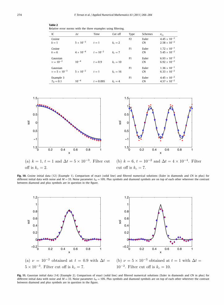
274 F. Ternat et al. / Applied Numerical Mathematics 61 (2011) 266–284
Table 2Relative error norms with the three examples using filtering.
IC �t Time Cut off Type Schemes eL2
Cosine F2 Euler 4.45 × 10⁻²
k = 1 5 × 10⁻³ t = 1 kc = 2 CN 2.58 × 10⁻²
Cosine F1 Euler 1.72 × 10⁻¹
k = 6 4 × 10⁻⁴ t = 10−2 kc = 7 CN 5.45 × 10⁻²
Gaussian F1 Euler 6.93 × 10⁻²
ν = 10−2 10−4 t = 0.9 kc = 10 CN 6.92 × 10⁻²
Gaussian F1 Euler 1.36 × 10⁻¹
ν = 5 × 10⁻³ 5 × 10⁻² t = 1 kc = 16 CN 6.33 × 10⁻²
Example 3 F1 Euler 4.45 × 10⁻²
T0 = 0.1 10−4 t = 0.095 kc = 4 CN 4.57 × 10⁻²
Fig. 10. Cosine initial data (12) (Example 1). Comparison of exact (solid line) and filtered numerical solutions (Euler in diamonds and CN in plus) fordifferent initial data with noise and M = 33. Noise parameter δm = 10%. Plus symbols and diamond symbols are on top of each other wherever the contrastbetween diamond and plus symbols are in question in the figure.
Fig. 11. Gaussian initial data (14) (Example 2). Comparison of exact (solid line) and filtered numerical solutions (Euler in diamonds and CN in plus) fordifferent initial data with noise and M = 33. Noise parameter δm = 10%. Plus symbols and diamond symbols are on top of each other wherever the contrastbetween diamond and plus symbols are in question in the figure.
F. Ternat et al. / Applied Numerical Mathematics 61 (2011) 266–284 275
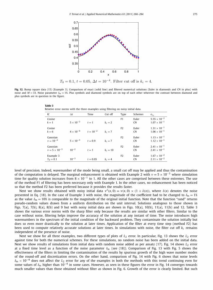
Fig. 12. Bump square data (15) (Example 3). Comparison of exact (solid line) and filtered numerical solutions (Euler in diamonds and CN in plus) withnoise and M = 33. Noise parameter δm = 1%. Plus symbols and diamond symbols are on top of each other wherever the contrast between diamond andplus symbols are in question in the figure.
Table 3Relative error norms with the three examples using filtering on noisy initial data.
IC �t Time Cut off Type Schemes eL2
Cosine F1 Euler 5.55 × 10⁻²
k = 1 5 × 10⁻³ t = 1 kc = 2 CN 1.07 × 10⁻¹
Cosine F2 Euler 1.31 × 10⁻¹
k = 6 4 × 10⁻⁴ t = 10−2 kc = 7 CN 1.06 × 10⁻¹
Gaussian F2 Euler 1.13 × 10⁻¹
ν = 10−2 5 × 10⁻³ t = 0.9 kc = 7 CN 1.12 × 10⁻¹
Gaussian F2 Euler 2.41 × 10⁻¹
ν = 5 × 10⁻³ 10−2 t = 1 kc = 10 CN 2.41 × 10⁻¹
Example 3 F2 Euler 1.67 × 10⁻²
T0 = 0.1 10−3 t = 0.05 kc = 4 CN 2.11 × 10⁻²
level of precision. Indeed, wavenumber of the mode being small, a small cut off may be applied and thus the contaminationof the computation is delayed. The marginal enhancement is obtained with Example 2 with ν = 5 × 10⁻³ where simulationtime for quality solution increases from 8 × 10⁻¹ to 1. All the other cases are comprised between these extremes. The useof the method F1 of filtering has been necessary only with Example 1. In the other cases, no enhancement has been noticedso that the method F2 has been preferred because it provides the results faster.
Next we show results obtained with noisy initial data vδ(x,0) = v(x,0) × (1 + δ(x)), where δ(x) denotes the noisepresented in Eq. (18). In the case of Example 3 with noise, the magnitude of the coefficient had to be changed to δm = 1%as the value δm = 10% is comparable to the magnitude of the original initial function. Note that the function “rand” returnspseudo-random values drawn from a uniform distribution on the unit interval. Solutions analogous to those shown inFigs. 7(a), 7(b), 8(a), 8(b) and 9 but with noisy initial data are shown in Figs. 10(a), 10(b), 11(a), 11(b) and 12. Table 3shows the various error norms with the sharp filter only because the results are similar with other filters. Similar to thecase without noise, filtering helps improve the accuracy of the solution at any instant of time. The noise introduces highwavenumbers in the spectrum of the initial condition of the backward problem. They contaminate the solution initially butdoes so even more drastically to the solution at later times. Application of the filter at every time step (method F2) hasbeen used to compute relatively accurate solutions at later times. In simulations with noise, the filter cut off kc remainsindependent of the presence of noise.
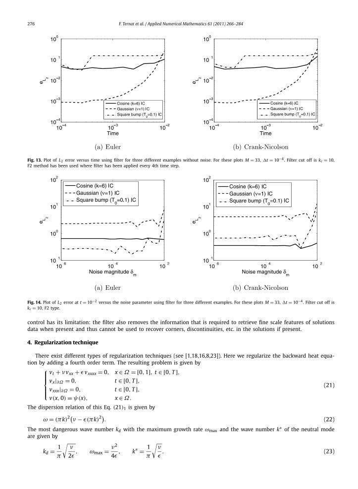
Next we show for all three examples, two different types of plots of L2 error. In particular, Fig. 13 shows the L2 erroragainst time for both the numerical schemes. For these simulations, no random noise has been added on the initial data.Next we show results of simulations from initial data with random noise added as per ansatz (17). Fig. 14 shows L2 errorat a fixed time level as a function of the noise parameter δm (see (18)). Comparison of Fig. 13 with Fig. 5 shows theeffectiveness of the filters in limiting the contamination of the results by spurious growth of the high wave number modesof the round-off and discretization errors. On the other hand, comparison of Fig. 14 with Fig. 6 shows that noise levelsδm < 10−4 does not affect the L2 error for any of the examples in both the methods with this trend continuing even forsome values of δm higher than 10−4 in some cases. However, as seen in these figures the error in Fig. 14 converges towardsmuch smaller values than those obtained without filter as shown in Fig. 6. Growth of the error is clearly limited. But such
276 F. Ternat et al. / Applied Numerical Mathematics 61 (2011) 266–284
Fig. 13. Plot of L2 error versus time using filter for three different examples without noise. For these plots M = 33, �t = 10−4. Filter cut off is kc = 10,F2 method has been used where filter has been applied every 4th time step.
Fig. 14. Plot of L2 error at t = 10−2 versus the noise parameter using filter for three different examples. For these plots M = 33, �t = 10−4. Filter cut off iskc = 10, F2 type.
control has its limitation: the filter also removes the information that is required to retrieve fine scale features of solutionsdata when present and thus cannot be used to recover corners, discontinuities, etc. in the solutions if present.
4. Regularization technique
There exist different types of regularization techniques (see [1,18,16,8,23]). Here we regularize the backward heat equa-tion by adding a fourth order term. The resulting problem is given by⎧⎪⎪⎨
⎪⎪⎩
vt + νvxx + εvxxxx = 0, x ∈ Ω = [0,1], t ∈ [0, T ],vx|∂Ω = 0, t ∈ [0, T ],vxxx|∂Ω = 0, t ∈ [0, T ],v(x,0) = ψ(x), x ∈ Ω.
(21)
The dispersion relation of this Eq. (21)1 is given by
ω = (πk)2(ν − ε(πk)2). (22)
The most dangerous wave number kd with the maximum growth rate ωmax and the wave number k∗ of the neutral modeare given by
kd = 1√
ν, ωmax = ν2
, k∗ = 1√
ν. (23)
π 2ε 4ε π ε
F. Ternat et al. / Applied Numerical Mathematics 61 (2011) 266–284 277
Fig. 15. Comparison of the exact (ω versus k) and numerical (|ρ|/�t versus k) dispersion relations for the regularized problem for several values of spaceand time steps. For these plots ν = 1 and kd = 10.
An appropriate choice of small value for the regularizing parameter ε can significantly curtail the spurious growth of shortwaves. We can see from the above formulas that we can equivalently treat kd or k∗ as regularizing parameter instead of εsince value of ε is automatically chosen if we choose either kd or k∗ . Next we discuss the schemes to be used for solvingthe above regularized problem.
4.1. Euler and CN schemes
Euler scheme. The finite difference equation for the regularized Eq. (21) is
D+t vn
m
�t= −ν
D+x D−
x vnm
�x2− ε
D+x D−
x D+x D−
x vnm
�x4, ∀m �= {1, M}, ∀n > 2. (24)
For numerical construction of the accurate solutions, it is also necessary to choose appropriate values of �x and �t sothat numerical and exact dispersion relations do not deviate too much from each other over a range of participating wavenumbers. Using the ansatz vn
m = ρneiξm (where ρ = eβ�t and ξ = kπ�x) in the finite difference equation (24) yields thedispersion relation
ρ = 1 + 4r sin2(
ξ
2
)− 16μ sin4
(ξ
2
), (25)
where μ = ε�t�x4 . Fig. 15(a) compares the exact (see Eq. (22)) and the numerical (see Eq. (25)) dispersion relations for several
choices of parameter values. This figure shows that optimal step sizes are �x = 10−4 and �t = 10−3 when ν = 1 andkd = 10. Note that with this set of parameters, the dispersion relation seems to be discontinuous in the range [12,26] of k.In fact, this is due to the representation in log scale of the function that reaches a value close to zero.
Crank–Nicolson scheme. The finite difference equation for the above regularized equation is
D+t vn
m
�t= − ν
2�x2
(D+
x D−x vn+1
m + D+x D−
x vnm
) − ε
2�x4
(D+
x D−x D+
x D−x vn+1
m + D+x D−
x D+x D−
x vnm
). (26)
For dispersion relation, the same ansatz for vnm as in the Euler scheme is inserted in the finite difference equation (26) of
the Crank–Nicolson scheme. This yields the following dispersion relation:
ρ = 1 + 2r sin2 (ξ2 ) − 8μ sin4 (
ξ2 )
1 − 2r sin2 (ξ2 ) + 8μ sin4 (
ξ2 )
. (27)
Fig. 15(a) compares the exact (see Eq. (22)) and the numerical (see Eq. (25)) dispersion relations for several choices ofparameter values. This figure shows that the optimal step sizes are �x = 10−4 and �t = 10−3 when ν = 1 and kd = 10.Since the plot is in log scale, note that sometimes the growth factor is undefined in a defined range of wavenumberbecause some values of ρ are less than zero.
278 F. Ternat et al. / Applied Numerical Mathematics 61 (2011) 266–284
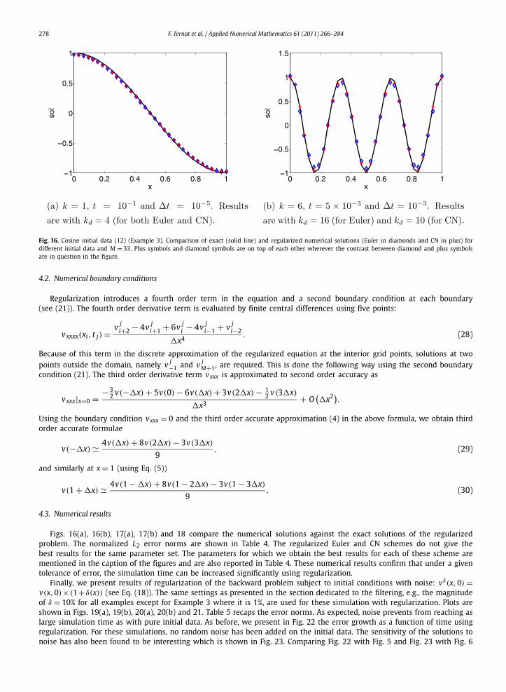
Fig. 16. Cosine initial data (12) (Example 3). Comparison of exact (solid line) and regularized numerical solutions (Euler in diamonds and CN in plus) fordifferent initial data and M = 33. Plus symbols and diamond symbols are on top of each other wherever the contrast between diamond and plus symbolsare in question in the figure.
4.2. Numerical boundary conditions
Regularization introduces a fourth order term in the equation and a second boundary condition at each boundary(see (21)). The fourth order derivative term is evaluated by finite central differences using five points:
vxxxx(xi, t j) = v ji+2 − 4v j
i+1 + 6v ji − 4v j
i−1 + v ji−2
�x4. (28)
Because of this term in the discrete approximation of the regularized equation at the interior grid points, solutions at twopoints outside the domain, namely v j
−1 and v jM+1, are required. This is done the following way using the second boundary
condition (21). The third order derivative term vxxx is approximated to second order accuracy as
vxxx|x=0 = − 32 v(−�x) + 5v(0) − 6v(�x) + 3v(2�x) − 1
2 v(3�x)
�x3+ O
(�x2).
Using the boundary condition vxxx = 0 and the third order accurate approximation (4) in the above formula, we obtain thirdorder accurate formulae
v(−�x) � 4v(�x) + 8v(2�x) − 3v(3�x)
9, (29)
and similarly at x = 1 (using Eq. (5))
v(1 + �x) � 4v(1 − �x) + 8v(1 − 2�x) − 3v(1 − 3�x)
9. (30)
4.3. Numerical results
Figs. 16(a), 16(b), 17(a), 17(b) and 18 compare the numerical solutions against the exact solutions of the regularizedproblem. The normalized L2 error norms are shown in Table 4. The regularized Euler and CN schemes do not give thebest results for the same parameter set. The parameters for which we obtain the best results for each of these scheme arementioned in the caption of the figures and are also reported in Table 4. These numerical results confirm that under a giventolerance of error, the simulation time can be increased significantly using regularization.
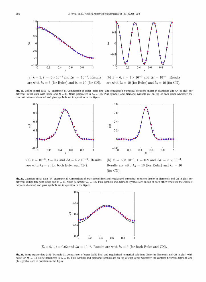
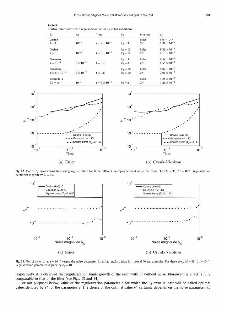
Finally, we present results of regularization of the backward problem subject to initial conditions with noise: vδ(x,0) =v(x,0)× (1+δ(x)) (see Eq. (18)). The same settings as presented in the section dedicated to the filtering, e.g., the magnitudeof δ = 10% for all examples except for Example 3 where it is 1%, are used for these simulation with regularization. Plots areshown in Figs. 19(a), 19(b), 20(a), 20(b) and 21. Table 5 recaps the error norms. As expected, noise prevents from reaching aslarge simulation time as with pure initial data. As before, we present in Fig. 22 the error growth as a function of time usingregularization. For these simulations, no random noise has been added on the initial data. The sensitivity of the solutions tonoise has also been found to be interesting which is shown in Fig. 23. Comparing Fig. 22 with Fig. 5 and Fig. 23 with Fig. 6
F. Ternat et al. / Applied Numerical Mathematics 61 (2011) 266–284 279
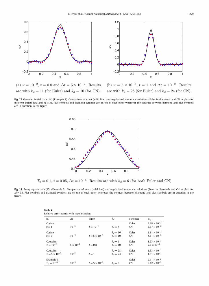
Fig. 17. Gaussian initial data (14) (Example 2). Comparison of exact (solid line) and regularized numerical solutions (Euler in diamonds and CN in plus) fordifferent initial data and M = 33. Plus symbols and diamond symbols are on top of each other wherever the contrast between diamond and plus symbolsare in question in the figure.
Fig. 18. Bump square data (15) (Example 3). Comparison of exact (solid line) and regularized numerical solutions (Euler in diamonds and CN in plus) forM = 33. Plus symbols and diamond symbols are on top of each other wherever the contrast between diamond and plus symbols are in question in thefigure.
Table 4Relative error norms with regularization.
IC �t Time kd Schemes eL2
Cosine Euler 3.18 × 10⁻²
k = 1 10−5 t = 10−1 kd = 4 CN 3.17 × 10⁻²
Cosine kd = 16 Euler 9.81 × 10⁻²
k = 6 10−3 t = 5 × 10⁻³ kd = 10 CN 4.81 × 10⁻²
Gaussian kd = 11 Euler 8.63 × 10⁻²
ν = 10−2 5 × 10⁻² t = 0.8 kd = 10 CN 7.6 × 10⁻²
Gaussian kd = 28 Euler 1.53 × 10⁻¹
ν = 5 × 10⁻³ 10−2 t = 1 kd = 24 CN 1.51 × 10⁻¹
Example 3 Euler 2.11 × 10⁻²
T0 = 10−1 10−5 t = 5 × 10⁻² kd = 6 CN 2.12 × 10⁻²
280 F. Ternat et al. / Applied Numerical Mathematics 61 (2011) 266–284
Fig. 19. Cosine initial data (12) (Example 1). Comparison of exact (solid line) and regularized numerical solutions (Euler in diamonds and CN in plus) fordifferent initial data with noise and M = 33. Noise parameter is δm = 10%. Plus symbols and diamond symbols are on top of each other wherever thecontrast between diamond and plus symbols are in question in the figure.
Fig. 20. Gaussian initial data (14) (Example 2). Comparison of exact (solid line) and regularized numerical solutions (Euler in diamonds and CN in plus) fordifferent initial data with noise and M = 33. Noise parameter δm = 10%. Plus symbols and diamond symbols are on top of each other wherever the contrastbetween diamond and plus symbols are in question in the figure.
Fig. 21. Bump square data (15) (Example 3). Comparison of exact (solid line) and regularized numerical solutions (Euler in diamonds and CN in plus) withnoise for M = 33. Noise parameter is δm = 1%. Plus symbols and diamond symbols are on top of each other wherever the contrast between diamond andplus symbols are in question in the figure.
F. Ternat et al. / Applied Numerical Mathematics 61 (2011) 266–284 281
Table 5Relative error norms with regularization on noisy initial conditions.
IC �t Time kd Schemes eL2
Cosine Euler 5.9 × 10⁻²
k = 1 10−5 t = 8 × 10⁻² kd = 3 CN 5.91 × 10⁻²
Cosine kd = 12 Euler 8.26 × 10⁻²
k = 6 10−4 t = 3 × 10⁻³ kd = 12 CN 7.13 × 10⁻²
Gaussian kd = 8 Euler 8.54 × 10⁻²
ν = 10−2 5 × 10⁻³ t = 0.7 kd = 8 CN 8.55 × 10⁻²
Gaussian kd = 10 Euler 8.02 × 10⁻²
ν = 5 × 10⁻³ 5 × 10⁻³ t = 0.8 kd = 10 CN 7.91 × 10⁻²
Example 3 Euler 1.21 × 10⁻²
T0 = 10−1 10−5 t = 2 × 10⁻² kd = 3 CN 1.21 × 10⁻²
Fig. 22. Plot of L2 error versus time using regularization for three different examples without noise. For these plots M = 33, �t = 10−4. Regularizationparameter is given by kd = 10.
Fig. 23. Plot of L2 error at t = 10−2 versus the noise parameter δm using regularization for three different examples. For these plots M = 33, �t = 10−4.Regularization parameter is given by kd = 10.
respectively, it is observed that regularization limits growth of the error with or without noise. Moreover, its effect is fullycomparable to that of the filter (see Figs. 13 and 14).
For our purposes below, value of the regularization parameter ε for which the L2 error is least will be called optimalvalue, denoted by ε∗ , of the parameter ε . The choice of the optimal value ε∗ certainly depends on the noise parameter δm

282 F. Ternat et al. / Applied Numerical Mathematics 61 (2011) 266–284
Fig. 24. Plot of L2 error at t = 2× 10⁻³ versus the regularization parameter ε with the cosine initial data (k = 1) for three values of the noise parameter δm .For these plots �t = 10−5 and M = 33.
which is a measure of signal to noise ratio modulo some constant depending on the examples. A strategy that will allowselection of ε∗ in dependency of the noise parameter δm is certainly helpful. However, it is not clear how to do this a priori.To get some insight into how to do this even a posteriori, plots of L2 error are shown against the regularization parameterε and the residual norm (‖ε × vxxxx‖2) in Figs. 24(a) and 24(b) respectively. The results are shown with CN scheme onlyand for the first example only because general trends of the plots for other combinations of the two methods and the threeexamples of this paper are similar. The plots in Fig. 24(a) resemble U -curves and those in Fig. 24(b) resemble L-curves. Itis worth mentioning here that L2 errors and the residual norms were computed for decreasing values of the regularizationparameter ε and then these plots were done. Therefore, it should be understood that the parameter ε decreases as any ofthe L-curves (including the one which looks more like a U for no noise case in Fig. 24(b)) is traced from right to left.
We see from the U -curves that both, the minimal value of L2 error (corresponding to ε∗) and the optimal value ε∗decrease monotonically with decreasing values of the noise parameter δm . From the L-curves, same inference is drawnabout the dependency of L2 error on the noise. However, notice that the effect of ε decreasing away from the optimal valueε∗ has much more dramatic effect on the L2 error than on the residual. In the presence of noise, L2 error increases rapidlywith hardly any change in the residual (the L-part of the L-curves). Therefore, either of the curves can be used for choosingthe optimal value ε∗ .
In general, smaller the magnitude of the noise, smaller the optimal value of the regularization parameter ε∗ . The valueof ε∗ seems to remain constant when the noise parameter reaches a value less than 0.01% (figure is not shown here).Indeed, for such a value of δm < 0.01% and such time level, the error is no longer affected by the noise in agreement withthe observation made in Fig. 6. As seen in the U -curves, for optimal choice ε∗ of the regularizing parameter with noiselevel δm < 0.01% in the initial data, the regularized solution approximates the exact one having an L2 error of the order ofO (10−3). In concluding this section, we want to emphasize that the discussion here on U - and L-curves is based on plotsmade from data obtained at a specific time level. More research is needed (which will be a topic of research in the future)to determine, even a posteriori, the optimal value of the regularizing parameter in dependency of time of simulation.
5. Discussion and conclusion
Two stable ways of computing solutions of backward heat equation, namely filtering (direct filtering of short waves)and regularization techniques (structural perturbation of the heat equation), have been proposed and discussed for theirproper implementation. For each of these ways of computing stable solutions, two finite difference methods, namely theEuler method and the Crank–Nicolson (CN) method, for solving the associated initial boundary value problem have beendevised. These schemes have been analyzed. In particular, (numerical) dispersion relations for these two numerical schemesassociated with each of the two initial boundary value problems arising in filtering and regularizing techniques respectivelyhave been derived.
Appropriate choice of parameters so that numerical dispersion relations well approximate the exact dispersion relationsof the PDEs over the range of participating wave numbers is one of the important factors in devising stable ways of com-puting the numerical solutions of the backward heat equation. This has been one of the hallmarks of the success of thesemethods which has been exemplified in this paper with adequate number of examples. Another important factor has beento apply the filter and set the level of the filter appropriately which are partly guided by severity of ill-posedness and partlyby trial and error. We have shown here that in this way, we are able to compute stable solutions for times longer than
F. Ternat et al. / Applied Numerical Mathematics 61 (2011) 266–284 283
otherwise possible. The methods are new. It will be interesting to see whether these results compare favorably or not withother existing methods [2,3,10,12,14,15,21,24] which is a topic of future research.
The filtering and regularization methods are used to obtain smooth approximate solutions of ill-posed problems. Thefiltering methods have been applied here in a way that can provide good approximate smooth solutions but falls shortof providing singular solutions such as the ones with corners and discontinuities. Such corners and discontinuities aresmoothed out in the solutions obtained by the way the filtering techniques are applied here. Singular solutions can be ob-tained by better applications of the filtering techniques which is difficult to apply in general because the application processinvolves in part science and in part art (see [13]). In the regularization technique, we have provided the U -curve criterionfor optimal choice of the regularizing parameter a posteriori. This optimal value is shown to decrease with decreasing noiselevel.
Acknowledgements
This paper has been made possible by a NPRP grant to one of the authors (Prabir Daripa) from the Qatar NationalResearch Fund (a member of The Qatar Foundation) and by a SCAT grant to the other two authors (Fabien Ternat and OscarOrellana). One of the authors (Fabien Ternat) thanks the Department of Mathematics at Texas A&M University for makinghis one month long summer visit to Dr. Daripa possible and enjoyable. He also thanks the Department of Mathematics atUniversidad Tecnica Federico Santa Maria, Valparaiso, Chile for making his research under SCAT grant possible. We wouldalso like to thank immensely the reviewers for their very constructive and insightful criticisms which have helps up toimprove the paper. The statements made herein are solely responsibility of the authors.
Appendix A. Definition of the filters used
We have applied five filters one of which is described in the main body of the text and the rest four are defined below:
1. Arctan filter Φa(k):
Φa(k) = 1
πarctan
(−104(k − kc)) + 0.5. (31)
2. Three polynomial filters Φi(k): smoothness of the sharp filter defined in the main body of the text can be improved byconsidering polynomial functions gi (see Daripa [4]):
Φi(k, p) =⎧⎨⎩
1, k � kc,
1 − gi(k), kc < k < k2,
0, k � k2,
(32)
where k = k−kck2−kc
. The smoothing functions are defined respectively by:
g1(x) = x, 0 < x < 1, (33)
g2(k) =
⎧⎪⎪⎪⎪⎪⎪⎨⎪⎪⎪⎪⎪⎪⎩
9
2x3, 0 < x � 1
3,
9x3 + 27
2x2 − 9
2x + 1
2,
1
3< x � 2
3,
1 − 9
2(1 − x)3,
2
3< x < 1,
(34)
g3(k) =
⎧⎪⎪⎪⎪⎪⎪⎪⎪⎪⎪⎪⎪⎪⎪⎨⎪⎪⎪⎪⎪⎪⎪⎪⎪⎪⎪⎪⎪⎪⎩
625
24x5, 0 < x � 1
5,
−625
6x5 + 3125
24x4 − 625
12x3 + 125
12x2 − 25
24x + 1
24,
1
5< x � 2
5,
625
4x5 − 3125
8x4 + 4375
12x3 − 625
4x2 + 775
24x − 21
8,
2
5< x � 3
5,
1 + 625
6(1 − x)5 − 3125
24(1 − x)4 + 625
12(1 − x)3 − 125
12(1 − x)2 + 25
24(1 − x) − 1
24,
3
5< x � 4
5,
1 − 625
24(1 − x)5,
4
5< x < 1.
(35)
These filters have varying degree of smoothness and how to apply these have been exemplified in gory detail inDaripa [4].

284 F. Ternat et al. / Applied Numerical Mathematics 61 (2011) 266–284
References
[1] K.A. Ames, L.E. Payne, Asymptotic behavior for two regularizations of the Cauchy problem for the backward heat equation, Mathematical Models andMethods in Applied Sciences 8 (1998) 187–202.
[2] L.D. Chiwiacowsky, H.F. De Campo Velho, Different approaches for the solution of a backward heat conduction problem, Inverse Problem Engineering 11(2003) 471–494.
[3] D.T. Dang, H.T. Nguyen, Regularization and error estimates for nonhomogeneous backward heat problems, Electronic Journal of Differential Equa-tions 2006-04 (2006) 1–10.
[4] P. Daripa, Some useful filtering techniques for ill-posed problems, Journal of Computational and Applied Mathematics 100 (1998) 161–171.[5] P. Daripa, H. Wei, A numerical study of an ill-posed Boussinesq equation arising in water waves and nonlinear lattices: Filtering and regularization
techniques, Applied Mathematics and Computation 101 (1999) 159–207.[6] J.J. Douglas, T.M. Gallie, An approximate solution of an improper boundary value problem, Duke Mathematical Journal 26 (1959) 339–347.[7] H. Engl, M. Hanke, A. Neubauer, Regularization of Inverse Probems, Kluwer Academic Publishers, 2000.[8] C.-L. Fu, X.-T. Xiong, Z. Qian, Fourier regularization for a backward heat equation, Journal of Mathematical Analysis and Applications 331 (2007) 472–
480.[9] K. Höllig, Existence of infinitely many solutions for a forward backward heat equation, Transactions of the American Mathematical Society 279 (1983)
299–316.[10] H. Houde, Y. Dongsheng, A non overlap decomposition method for the forward-backward heat equation, Journal of Computational and Applied Math-
ematics 159 (2003) 35–44.[11] F. John, Numerical solution of the equation of heat conduction for preceding times, Annali di Matematica Pura et Applicata Series IV 40 (1955) 129–142.[12] L. Kentaro, Numerical solution of backward heat conduction problems by a high order lattice-free finite difference method, Journal of the Chinese
Institute of Engineers 27 (2004) 611–620.[13] R. Krasny, A study of singularity formation in a vortex sheet by the point-vortex approximation, Journal of Fluid Mechanics 167 (1986) 65–93.[14] D. Krawczyk-Stando, M. Rudnicki, Regularization parameter selection in discrete ill-posed problems – the use of the u-curve, International Journal of
Applied Mathematics and Computer Sciences 17 (2007) 157–164.[15] N.S. Mera, The method of fundamental solutions for the backward heat conduction problem, Inverse Problems in Science and Engineering 13 (2005)
65–78.[16] N.S. Mera, L. Elliot, D.B. Ingham, An inversion method with decreasing regularization for the backward heat conduction problem, Numerical Heat
Transfer, Part B 42 (2002) 215–230.[17] W. Miranker, A well posed problem for the backward heat equation, Proceedings of the American Mathematical Society 12 (1961) 243–247.[18] W.B. Muniz, F.M. Ramos, H.F. De Campos Velho, Entropy- and Tikhonov-based regularization techniques applied to the backwards heat equation,
Computers and Mathematics with Applications 40 (2000) 1071–1084.[19] J. Nash, Continuity of solutions of parabolic and elliptic equations, American Journal of Mathematics 80 (1958) 931–954.[20] C. Pucci, Sui problemi di Cauchy non “ben posti”, Atti Accademia Nazionale dei Lincei. Rend. Classe di Scienze Fisiche, Matematiche e Naturali 18
(1955) 473–477.[21] A. Qian, C.-L. Fu, R. Shi, A modified method for a backward heat conduction problem, Applied Mathematics and Computation 185 (2007) 564–573.[22] I. Seidman, Optimal filtering for the backward heat equation, SIAM Journal of Numerical Analysis 33 (1996) 162–170.[23] G. Teschke, M. Zhariy, M.J. Soares, A regularization of nonlinear diffusion equations in a multiresolution framework, Mathematical Methods in the
Applied Sciences 31 (2008) 575–587.[24] X.-T. Xiong, C.-L. Fu, A. Qian, Two numerical methods for solving a backward heat conduction problem, Applied Mathematics and Computation 179
(2006) 370–377.