two-phase flow investigations of gas-kick scenarios
TRANSCRIPT

University of Leoben
Doctoral Thesis
Two-Phase Flow Investigations of
Gas-Kick Scenarios
Application of Computational Fluid Dynamics to Kick Analysis in Wellbores
Claudia Carina Gruber
A thesis submitted in partial fulfilment of the requirements for the degree of
“Doktor der montanistischen Wissenschaften”
Leoben, May 2016


I
I declare in lieu of oath, that I wrote this thesis and performed the associated
research myself, using only literature cited in this volume.
……………………………………………………………
Claudia Gruber, Leoben, May 2016

II
DANKSAGUNG
Viele Menschen haben dazu beigetragen, dass diese Dissertation entstehen konnte.
Herrn Prof. Wilhelm Brandstätter möchte ich für die Betreuung dieser Arbeit danken, sowie
für die Möglichkeit der mittlerweile langjährigen Mitarbeit in seinem Arbeitskreis. Durch ihn
erhielt ich viele interessante Einblicke in die angewandte Thermofluiddynamik und konnte
mir durch seine Unterstützung eine gut fundierte Wissensbasis aneignen. Er hat diese Arbeit
in vielfältiger Weise unterstützt, nicht zuletzt auch in organisatorischer und menschlicher
Hinsicht.
Im Besonderen möchte ich mich bei Prof. Gerhard Thonhauser für die freundliche
Unterstützung zur Fertigstellung dieser Arbeit bedanken. Ich danke Herrn Dr. Hermann
Spörker für die Initiative sowie der OMV für die finanzielle Unterstützung dieser Arbeit. Des
Weiteren möchte ich mich bei allen Mitarbeitern des Lehrstuhls für die gute und freundliche
Arbeitsatmosphäre bedanken, die ich stets sehr zu schätzen wusste.
Mein besonderer Dank gilt meiner Familie. Im Speziellen meinen beiden Kindern, Ines und
Daniel. Die für mich stets eine große Unterstützung waren, und mir den nötigen Antrieb
gaben diese Arbeit fertigzustellen.

III
ABSTRACT
Common approaches in kick modeling are based on the assumption of a more or less single
“gas bubble” present in the annulus and slowly migrating upwards after shut-in. While this
assumption satisfies straightforward volumetric well control aspects, it ignores species
transport and chemical reaction kinetics leading to drill string corrosion. Especially when
dealing with sour gas influxes, the assessment of corrosive damage to high-strength drill
string components caused by sulfide stress cracking becomes essential. Therefore a better
insight on the flow morphology and associated mechanisms during a kick event is needed to
assess the associated corrosive risk.
The aim of the work presented in this thesis is to provide a better understanding of the two-
phase flow situation resulting from selected kick scenarios. A Computational Fluid Dynamics
(CFD) approach was chosen to simulate the dissolution and distribution of influx gas. The
selection of a two-phase flow model within CFD is usually based on the expected flow
pattern. Since a gas-kick is a fundamentally transient event accompanied by many unknowns
the intention was not to make any a-priory assumptions regarding the evolving flow field.
Consequently the focus was put on a spatially highly resolved computational model combined
with the application of the Volume of Fluid Method. Thereby no restriction on specific flow
patterns was active and two-phase interactions could be observed at a close-up view. However
the involved computational costs demanded a limitation in model size to the near bottom-hole
section of the wellbore. This section shows certain characteristics that are dominated by the
inflow conditions of the gas as well as by the configuration of the mud stream entering the
annulus.
Several inflow scenarios are investigated and methodologies are described to characterize
flow aspects that are of potential interest to corrosion engineers. One of the major difficulties
in modeling the corrosive risk to the drill string during a gas-kick is the determination of
liquid-gas phase interface. As mass transfer and significant chemical reactions are related to
the size of the phase interface area, a sound estimate of the same is of utmost importance.
Simulation results illustrate two-phase flow morphology and associated specific phase
interface area, as well as local mass transfer coefficients and the distribution of dissolved gas.
The transient and spatial change of flow patterns in a wellbore during a kick event is
discussed. It is explained how the flow pattern is affected by gas expansion and how it may be
influenced by gas dissolution. Finally based on the findings of the detailed simulation studies,
a coarser full scale kick modeling approach covering the entire wellbore is suggested.

IV
ZUSAMMENFASSUNG
Bei der Modellierung von plötzlichen Gaseintritten in Bohrlöchern wird oftmals von der
Annahme ausgegangen, dass sich das eingetretene Gas nach Verschluss des Bohrlochs wie
eine zusammenhängende Blase verhält während ihres Aufstiegs im Ringspalt. Für eine rein
volumetrische Betrachtungsweise ist diese Annahme ausreichend, allerdings werden hierbei
der Transport chemischer Spezies und mögliche chemische Reaktionen welche zu
Korrosionsschäden am Bohrstrang führen nicht berücksichtigt. Vor allem wenn Sauergas bei
der Bohrung angetroffen wird, ist es wesentlich den möglichen Schaden bedingt durch
Spannungsrisskorrosion am aus hoch-festen Stählen bestehenden Bohrgestänge abzuschätzen.
Folglich ist klares Verständnis der Strömungsverhältnisse, und damit verbundenen Vorgänge
während eines Gaseintritts, zur besseren Einschätzung eines etwaigen Korrosionsrisikos
notwendig.
Ziel der vorliegenden Arbeit ist es, ein besseres Verständnis für die gegenständliche
Zweiphasenströmung anhand ausgewählter Kick-Szenarien zu vermitteln. Mittels
numerischer Strömungssimulation wird die Phasenverteilung und Löslichkeit des Gases
berechnet. Grundsätzlich erfolgt die Auswahl eines geeigneten Zweiphasen-
Modellierungsansatzes basierend auf einer a-priori Annahme der Strömungsverhältnisse. Da
es sich bei einem plötzlichen Gaseintritt allerdings um ein fundamental transientes Ereignis
begleitet von diversen Unbekannten handelt ist von einer Vorwegnahme oder Einschränkung
des Strömungsbildes abzusehen. Der Einsatz eines hoch-auflösenden Berechnungsgitters in
Verbindung mit der Volume of Fluid Methode ermöglicht eine detailreiche und
uneingeschränkte Nachbildung beliebiger Strömungsmuster. Allerdings verlangt der damit
verbundene erhöhte Berechnungsaufwand eine Einschränkung in der Modellgröße auf den
unmittelbaren Bereich ab Bohrlochsohle. Dieser Abschnitt des Bohrlochs zeigt besondere
Strömungscharakteristika aufgrund des Gaseintritts sowie der Strömungsmuster bedingt durch
die Umlenkung der Bohrspülung.
Verschiedene Gaseintrittsszenarien werden untersucht und Methoden zur Charakterisierung
korrosionsrelevanter Strömungsparameter beschrieben. Die Bestimmung der
Phasengrenzfläche zwischen Bohrspülung und Gas stellt dabei die größte Herausforderung
dar. Eine möglichst genaue Bestimmung der Phasengrenzfläche ist deshalb so bedeutend, da
mit ihrer Ausdehnung wesentliche Mechanismen wie Stoffübergang und chemische
Reaktionen korrelieren. Die Simulationsergebnisse illustrieren das Erscheinungsbild der
Zweiphasenströmung, sowie die damit verbundene Phasengrenzfläche, die lokalen
Stoffaustauschkoeffizienten und die Verteilung des gelösten Gases. Die zeitliche und örtliche
Änderung der Strömungsmuster im Bohrloch während eines plötzlichen Gaseintritts wird
diskutiert. Der Einfluss der Dichteänderung der aufsteigenden Gases sowie der Gaslöslichkeit
auf das Erscheinungsbild der Strömung wird beschrieben. Basierend auf den Erkenntnissen
der Detailstudien wird ein möglicher Ansatz zur Modellierung des gesamten Bohrlochs
vorgeschlagen.

V
für Ines und Daniel
VI
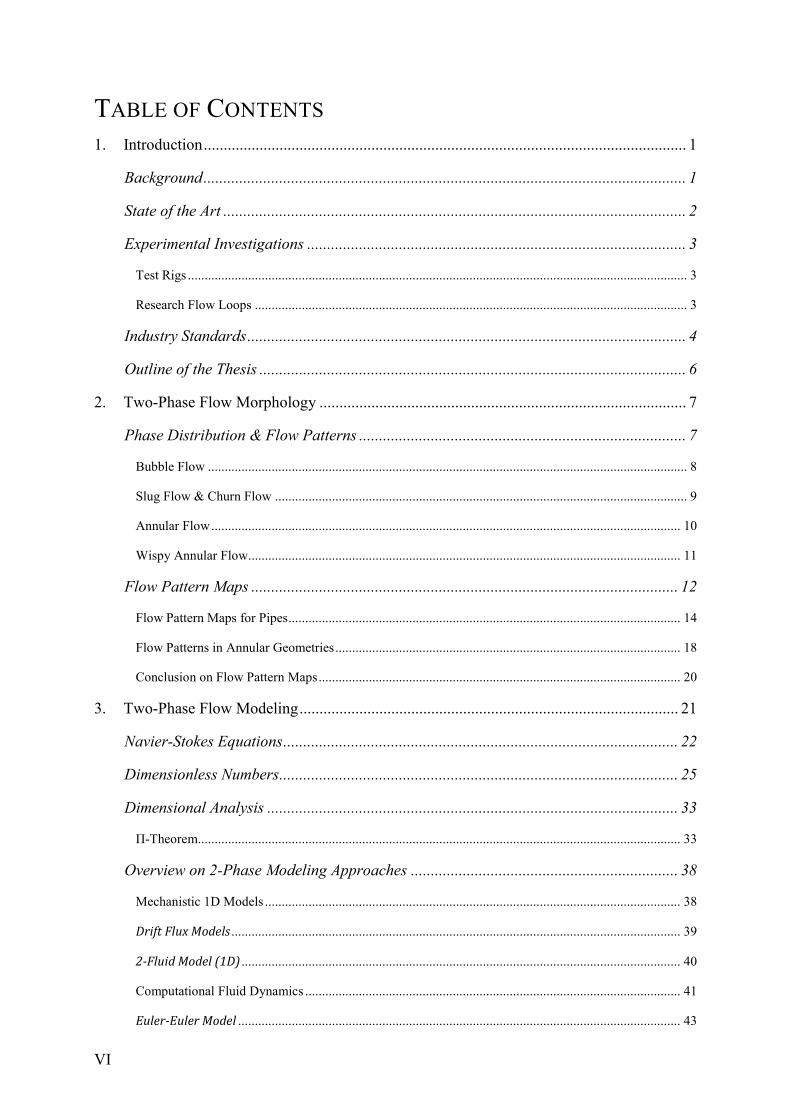
TABLE OF CONTENTS
1. Introduction ......................................................................................................................... 1
Background ......................................................................................................................... 1
State of the Art .................................................................................................................... 2
Experimental Investigations ............................................................................................... 3
Test Rigs ..................................................................................................................................................... 3
Research Flow Loops ................................................................................................................................. 3
Industry Standards .............................................................................................................. 4
Outline of the Thesis ........................................................................................................... 6
2. Two-Phase Flow Morphology ............................................................................................ 7
Phase Distribution & Flow Patterns .................................................................................. 7
Bubble Flow ............................................................................................................................................... 8
Slug Flow & Churn Flow ........................................................................................................................... 9
Annular Flow ............................................................................................................................................ 10
Wispy Annular Flow................................................................................................................................. 11
Flow Pattern Maps ........................................................................................................... 12
Flow Pattern Maps for Pipes ..................................................................................................................... 14
Flow Patterns in Annular Geometries ....................................................................................................... 18
Conclusion on Flow Pattern Maps ............................................................................................................ 20
3. Two-Phase Flow Modeling ............................................................................................... 21
Navier-Stokes Equations ................................................................................................... 22
Dimensionless Numbers .................................................................................................... 25
Dimensional Analysis ....................................................................................................... 33
Π-Theorem................................................................................................................................................ 33
Overview on 2-Phase Modeling Approaches ................................................................... 38
Mechanistic 1D Models ............................................................................................................................ 38
Drift Flux Models ...................................................................................................................................... 39
2-Fluid Model (1D) ................................................................................................................................... 40
Computational Fluid Dynamics ................................................................................................................ 41
Euler-Euler Model .................................................................................................................................... 43

VII
Euler Lagrangian Approach .................................................................................................................... 44
Euler Spatial DNS Approach .................................................................................................................... 45
Multi-Phase Flow Simulators ........................................................................................... 49
4. Corrosion Issue in Drilling ................................................................................................ 50
Corrosion Modeling .......................................................................................................... 51
Sulfide Stress Cracking ..................................................................................................... 52
Influence of Flow Field on Corrosion .............................................................................. 53
Corrosion Modeling Approach ......................................................................................... 55
Gas Solubility ........................................................................................................................................... 55
Mass Transfer Formulation ....................................................................................................................... 57
5. Modeling Approach .......................................................................................................... 63
Simulation Tool ................................................................................................................. 64
Model Setup and Boundary Conditions ............................................................................ 64
Model Geometry ....................................................................................................................................... 64
Multiphase Flow Model ............................................................................................................................ 65
Turbulence Modeling & Grid Considerations .......................................................................................... 67
Representation of Drill Bit ........................................................................................................................ 70
Drilling Mud Circulation .......................................................................................................................... 71
Influence of Rotation ................................................................................................................................ 72
Pressure Situation ..................................................................................................................................... 74
Kick-Gas Inlet Condition .......................................................................................................................... 77
Modeling of Gas Dissolution .................................................................................................................... 83
6. Results and Discussion ..................................................................................................... 90
Quantification of Two Phase Flow ................................................................................... 90
Velocity Data ............................................................................................................................................ 91
Void fraction ............................................................................................................................................. 94
Simulated Kick Scenarios ................................................................................................. 95
Location of Kick Entrance ........................................................................................................................ 97
Lateral Kick Scenario – Single Fracture .................................................................................................. 97
Bottom-Hole Kick Scenario – Multiple Fractures ................................................................................. 112

VIII
Loss of Mud Circulation ......................................................................................................................... 123
Lateral Kick Scenario – Cavernous Opening ......................................................................................... 123
Bottom-Hole Kick Scenarios .................................................................................................................. 128
7. Conclusions ..................................................................................................................... 136
Suggestions for Future Work .......................................................................................... 138
Bibliography ........................................................................................................................... 141

Two-Phase Flow Investigations of Gas-Kick Scenarios
Chapter 1: Introduction
1
1. Introduction
Background
During drilling operations the control of the well at all times is of utmost importance.
Consequences of a loss in well control can be devastating for the drilling rig, the crew and the
environment. The loss of well control can be initiated by the inflow of formation fluids into
the well encountered when drilling into formations with pressures higher than anticipated.
Such a fluid intrusion is called a kick.
Gas-kicks are especially dangerous because gas reduces the wellbore pressure more quickly
than liquids do and confinement at the surface is more difficult. Thus, gas-kicks more often
result in loss of well control and in surface fires and explosions. Therefore formation fluids
that have flowed into the wellbore and begin displacing the drilling fluid must be removed
quickly. Emergency procedures to manage the unexpected inflow and its effects are referred
as well-control operations. Common procedures like “wait and weight” and drillers method
have been applied successfully over decades to remove formation fluids from the wellbore.
However the physical phenomena occurring thereby are still purely understood, in particular
the movement and distribution of the kick fluids as they are pumped to the surface. Often kick
detection methods are too slow and inaccurate. Several minutes may elapse before a kick is
detected at the surface. During this time a considerable amount of gas may find its way into
the wellbore and can cause a hazardous situation.
Apart from the efforts taken to regain well control, a kick can also have a considerable impact
with respect to corrosion. The inflow of formation fluid may even be so low and occurring
continuously that it is not identified directly as a kick but still poses an issue in terms of
corrosion. Numerous conditions encountered during drilling operations cause corrosion to the
drilling equipment and can be differentiated by their nature of attack.
In hydrocarbon reservoirs large quantities of hydrogen sulfide (H2S) are often encountered,
especially when drilling deep wells. Hydrogen sulfide is known to induce and/or accelerate
the rate of cracking of high strength steels in acidic, aqueous environments due to the
migration of atomic hydrogen into the metal lattice and subsequent recombination to
hydrogen modules. This type of metal deterioration is called sulfide stress-cracking (SSC) and
is typical for steels above certain yield strength. Generally the higher the yield strength, the
more susceptible the steel will be to SSC.
Naturally sulfide stress-cracking is extremely important in oil and gas production. Drilling
operations are faced with a requirement for high-strength steel tubulars, which should
generally not come in contact with sour reservoir fluids, but will potentially be exposed to
high H2S concentrations when influxes of reservoir fluids are taken. Casing and tubing
materials for wells expected to produce sour fluids are selected based on the principles and
recommendations of the NACE MR0175 standard. The selection process is based on the

Two-Phase Flow Investigations of Gas-Kick Scenarios
Chapter 1: Introduction
2
drilling mud type, the H2S partial pressure, the system pressure and the gas to oil ratio in the
system.
Since presence of a “sour” environment depends on the H2S partial pressure, the trend to
deeper and higher-pressure wells leads to even small concentrations of H2S in the reservoir
gas triggering this threshold level. At the same time, the requirement to access deeper
reservoirs triggers a necessity of utilizing high-strength drill pipe while at the same time
assessing and controlling the risks stemming from potentially exposing these high-strength
steels to sour wellbore environments. Naturally there is considerable economic interest to
estimate the need of equipment exchange and/or define accurate limits for the use of drill pipe
equipment in such environments.
State of the Art
Kick detection and killing methods have changed very little over the years. The traditional
way to detect kicks is to monitor the drilling mud balance and the change in pit volume. Flow
measurements are often done indirectly by multiplying the number of pump strokes with the
pumps volumetric displacement. This approach is rather inaccurate and has the disadvantage
that kicks are detected rather late and small kicks may even remain undetected. Once a kick is
detected, corrective action is taken to regain control over the well. The well is shut in and a
kick killing procedure is launched. The driller has to make decisions under intense stress.
Mistakes in the design of the killing strategy can lead to formation damage or loss of the well.
Due to the slow kick detection method a considerable amount of gas has already entered the
wellbore and needs to be safely circulated out of the wellbore.
Although a considerable amount of work has been done in well control, little attention has
been given to the issue of multiphase flow mechanisms during a gas-kick. Experimental
investigations at flow loops such as Schlumberger Cambridge Research Center have shown
that during a simulated kick, the incoming gas rises in a complex way and does not occupy
the entire cross section of the annular channel.
Numerous kick simulators have the capability to model various kick sizes and intensities for
any given geometry. These simulators are extremely useful in predicting pressure profiles
during the kick removal circulation. By doing so many kick simulators model the kick as a
single bubble migrating upward as a single slug. Any mixing between the formation fluid and
the drilling mud is neglected. These simulators are good in predicting the pressure profiles
during well control operations but lack the description of multiphase flow phenomena. Such
phenomena include the description of the movement of each individual phase, the evolution
and deformation of the phase interface, and phase exchange processes such as the dissolution
of gas in the liquid and associated corrosion risks.
Two-Phase Flow Investigations of Gas-Kick Scenarios
Chapter 1: Introduction
3
Experimental Investigations
Extensive physical experiments simulating gas-kicks, both academic and by the oil and gas
industry, have been conducted using flow loops and test apparatus. Among these only a few
will be mentioned in this chapter based on their relevance to the subject of this work.
Test Rigs
During the 1980’s and 1990’s several full scale gas-kick experiments have been performed by
Rogaland Research Institute (RRI), nowadays known as IRIS, in a 2020 m long and 63
degrees inclined research well at ULLRIGG. Ullrigg is a full size offshore-style triple rig,
located onshore at Ullandhaug in Stavanger, Norway. The site contains 7 different test wells
and was founded 1982 by Shell for research purposes. The gas-kick experiments were carried
out with air/water-based mud as well as nitrogen/oil-based mud. The gas was injected into the
well at a controlled rate through a coiled tubing at the bit. Experiment parameters like mud
density, gas concentration, gas type, mud flow rate, injection depth, and mud type were
varied. The active pit volume, standpipe pressure and return mud flow rate were logged
during the experiments. The main focus of the research project laid on improvement of safety
during drilling by data analysis and development of new kick detection methods. The tests
were conducted to gain a better understanding of the kick process and provided important
implications regarding kick detection and well control, see Rommetveit et al. (1989) and
Hovland (1992).
Research Flow Loops
Compared to experiments conducted at test rigs, experimental setups at research flow loops
mostly located at Universities and or national research centers generally provide a higher
grade of information due to the intensive measurement infrastructure. However these research
flow loops are limited in size and applicable pressure conditions.
Intensive research was done at the Schlumberger Cambridge Research (SCR) focusing on
two phase flow characteristics. The multiphase flow loop test facility built in 1985 at SCR
offers a straight flow length of almost 12 m with a 9.5 m section permitting visual evaluation
of the flows. The piping is mounted on a 15 m long table which can be pivoted, enabling tests
to be carried out in all orientations from horizontal to vertical. The facility is designed to
operate at pressures up to 10 bars. Johnson et al. (1991, 1993) preformed tests on gas
migration velocities in this realistic drilling geometry with rheological accurate drilling fluids
in inclined and vertical. The majority of the tests were made with a polymer mud analogue
which permitted visual observations of the flow field. Their results showed that the gas rises
faster than previously believed and that kicks will rise faster in a viscous drilling mud than in
water. This is due to a change in the flow pattern causing the formation of large slug-type
bubbles. Gas rise velocity and bubble size is independent of void fraction. They also reported
significant differences between the effect of deviation on gas migration characteristics in pipe
and annular flows.

Two-Phase Flow Investigations of Gas-Kick Scenarios
Chapter 1: Introduction
4
Of certain interest is the transient two-phase flow test facility TOPFLOW located at the
Helmholtz-Zentrum Dresden-Rossendorf (HZDR). The facility was designed to investigate
steady-state and transient two-phase flows at realistic operational parameters. Numerous two-
phase flow experiments are planned and executed in close collaboration with the
Computational Fluid Dynamics (CFD) community for the evaluation of multiphase flow
models. The testing facilities are highly instrumented and equipped with wire-mesh sensors
which make them ideally suited for the purpose of model development and CFD code
validation. CFD grade experiments as conducted at HZDR are usually very rare.
SINTEF multiphase laboratory facilities located in Trondheim, Norway: These laboratories
are especially designed to gain knowledge about the link between chemistry and fluid
mechanics. SINTEF operates several multiphase flow loops of different scales to provide flow
assurance related research for the petroleum industry. It is the world’s largest flow laboratory
and is financed by industry as well as public contracts and the research council of Norway.
The development of the OLGA multiphase pipe flow simulator was continued and
experimentally verified in this institution.
H2S related corrosion is a topic of great concern but poses difficulties to be studied in the
laboratory due to the hazardous nature of H2S. Especially for the case of sour gas entering a
wellbore at pressures of 20 MPa and more it is impossible to carry out similar experimental
investigations on a flow-loop. Both the high absolute pressure needed and the aggressive
nature of hydrogen sulfide prohibits such investigations. The Institute for Corrosion and
Multiphase Technology at the University of Ohio is probably the only institution who owns a
hydrogen sulfide multiphase testing facility. The environmentally isolated corrosion flow loop allows investigations of the erosion-corrosion process in sour gas environments. Gas mixtures
of methane, nitrogen, and/or carbon dioxide are mixed with flowing liquid mixtures of water
and/or oil producing flow regimes of stratified flow, slug flow, or annular flow in the
multiphase environment. Three separate test sections for corrosion monitoring where various
types of corrosion-monitoring equipment can be installed are available. The flow loop can be
operated at system temperatures ranging from 40°C to 90°C and pressures from atmospheric
to 70 bars. The system allows investigating the influence of various concentrations of
hydrogen sulfide gas on corrosion rate in a controlled multiphase environment.
Industry Standards
The information gathered by the oil and gas production industry on the handling of H2S-
containing process streams is summarized in several standards for material requirements (MR
standards) and test methods (TM standards). These standards are published by the worldwide
corrosion authority NACE (National Association of Corrosion Engineers).
Among them is the NACE MR0175 or ISO 15156, which gives requirements and
recommendations for the selection and qualification of carbon and low-alloy steels, corrosion-
resistant alloys, and other alloys for service in equipment used in oil and natural gas
production and natural gas treatment plants in H2S-containing environments, whose failure
could pose a risk to the health and safety of the public and personnel or to the equipment

Two-Phase Flow Investigations of Gas-Kick Scenarios
Chapter 1: Introduction
5
itself. The standard delineates the partial pressures and conditions under which sulfide stress-
cracking can be expected and sets forth a list of materials suitable for handling sour gases and
aqueous streams.
Figure 1: Effect of H2S on Sulfide Stress Cracking, NACE
Another important standard is MR0103-2012, which defines material requirements for
resistance to sulfide stress cracking (SSC) in sour refinery process environments. One of the
types of material damage that can occur as a result of hydrogen charging is sulfide stress
cracking (SSC) of hard weldments and microstructures, which is addressed by this standard.
This standard is intended to be utilized by refineries, equipment manufacturers, engineering
contractors, and construction contractors.

Two-Phase Flow Investigations of Gas-Kick Scenarios
Chapter 1: Introduction
6
Outline of the Thesis
Subject of this thesis is to investigate the ability of a Computational Fluid Dynamics (CFD)
based approach to simulate the distribution of influx gas in the drilling fluid during kick
situations. Special focus is put on the bottom-hole inlet region of a vertical well, with the aim
of obtaining a highly resolved phase distribution. The modeling approach has to be able to
describe the unsteady motion of a compressible gas phase, taking into account turbulence as
well as non-Newtonian rheology and no a priori assumptions regarding flow patterns are
allowed. The outcome of this investigation shall provide a basis for a subsequent modeling
effort covering the chemical reaction kinetics with respect to H2S influxes in high-pH drilling
fluid environments. This thesis builds a basis for a sound understanding of the complex two-
phase flow morphology and associated mechanisms, which is needed to establish an adequate
model for corrosion risk assessment.
This thesis begins with an introduction to two-phase flow and its characteristics. In chapter 2
typical flow patterns in two-phase flow in vertical pipes are described. The commonly known
concept of flow pattern maps is illustrated and its advantages and disadvantages are discussed.
Chapter 3 deals with multiphase flow modeling approaches. The basic definition of the
governing flow equations for single phase flow is given. It is explained how a fluid-
mechanical problem can be analyzed based on dimensionless numbers. Next the concept of
dimensional analysis is elucidated and a selection of dimensionless groups defining the
problem at hand is suggested. After this an overview of two-phase flow modeling approaches
according to their complexity is provided. Beginning with 1-d mechanistic models up to
multiphase flow modeling approaches in Computational Fluid Dynamics. The issue of
corrosion in drilling engineering is summarized and discussed in chapter 4. The actual
modeling approach and model setup for the numerical simulation of gas-kick scenarios is
described in chapter 5. Results and discussion of the conducted simulation cases is given in
chapter 6. Finally project conclusions and recommendations for future work are provided in
the last chapter.

Two-Phase Flow Investigations of Gas-Kick Scenarios
Chapter 2: Two-Phase Flow Morphology
7
2. Two-Phase Flow Morphology
Single-phase flow can be classified according to the external geometry of the flow channel as
well whether the flow is laminar or turbulent. In contrast multiphase flow is classified
according to the internal phase distributions or morphology of the flow. In general multiphase
flow is defined as the concurrent or countercurrent movement of two or more immiscible
phases, which can be solid, liquid or gas. Each phase can consist of several chemical
components.
In this work only two-phase flows of gas and liquid are considered. The associated physical
phenomena are especially complex, since they combine the characteristics of a deformable
interface and the compressibility of one of the phases. Gas-liquid flows play an important role
in many industrial processes and can cover a wide spectrum of different scales. However any
two-phase flow is characterized by a moving boundary between the phases. Geometry, fluid
properties and boundary conditions effect the geometric distribution of the phases within the
flow and hence the interfacial area available for mass, momentum or energy exchange
between the phases. Moreover, the flow within each phase will clearly depend on that
geometric distribution. This illustrates the complicated two-way coupling between the flow in
each of the phases and the geometry of the flow. The complexity of this two-way coupling
presents a major challenge in the study of two-phase flows.
Phase Distribution & Flow Patterns
The most difficult thing in multiphase flow simulation is the prediction of the phase
distribution and phase interface. The phase interface is the boundary between bulk regions of
two fluids. The interface is a region where physical quantities vary continuously but it’s
extend is only of a few molecules. Therefore it is a practical concept to consider a so-called
“functional interface” with a zero thickness and a jump in physical properties across it. The
detection and tracking of the phase interface in multiphase flow can only be accomplished by
the means of Computational Fluid Dynamics. Nevertheless this poses a challenging modeling
task and is naturally very computationally intensive and still quite limited. It may be possible
at some time in the future to compute the Navier-Stokes equations for each of the phases and
to resolve every detail of a multiphase flow but with current capabilities we are still far from
this.
Before appropriate computational power was available researches introduced flow pattern
maps for the qualitative description and classification of phase distribution in their models.
When observing gas-liquid flow in a given channel the distribution of the phase interface can
be of any arbitrary form. But researchers soon noticed that these forms can be summarized
into a few types of interfacial distribution and used for classification of multiphase flow.
Thereby a particular type of geometric phase distribution is termed flow. Detailed discussions
of these patterns are given by Hewitt (1982), Whalley (1987) and Dukler and Taitel (1986).
The macroscopic behavior of the flow like pressure drop, wall heat exchanges or mechanical

Two-Phase Flow Investigations of Gas-Kick Scenarios
Chapter 2: Two-Phase Flow Morphology
8
interaction with structures is strongly correlated to the flow pattern and can vary from one
pattern to another. Almost all multiphase flow models are based on the concept of flow
patterns. This is of great ease for modeling but also introduces the disadvantage of
discontinuities between the individual flow pattern types.
It is necessary to define flow patterns independently for vertical and horizontal channel
orientation. In vertical pipes, two-phase flow can be classified into four flow patterns:
Bubble flow
Slug flow
Churn flow
Annular flow
Bubble Flow Slug Flow Churn Flow Wispy Annular Flow Annular Flow
Figure 2: Flow Patterns in Vertical Flow (G.F. Hewitt)
The flow pattern depends on the fluid properties, the size of the conduit and the flow rates of
each of the phases. The flow pattern can also depend on the configuration of the inlet. It can
take some distance for the flow pattern to fully develop and the flow pattern can change with
distance. This is certainly true for a well-bore, where the change in pressure affects the gas
density and consequently alters the gas flow rate. For fixed flow conditions and fluid
properties, the flow rates are the independent variables that can be correlated to a certain flow
pattern.
Bubble Flow
Initially when gas is introduced into a liquid, bubbles are generated. The size of bubbles
detaching from the bubble source depends on the geometrical properties of the inlet (e.g.
diameter of holes) as well as on the gas and liquid properties and the gas flow rate. The
bubble size is typically much smaller than the diameter of the tube. Bubble flow is observed at
low superficial gas velocities. In this case gas is the dispersed phase. One of the most
important features of dispersed flows is that mass, momentum and energy transfer between
the phases are carried out from each bubble to the surrounding continuous phase. Therefore,
the mechanisms of mass, momentum and energy transfer from a single bubble basically
control the interaction between phases. The most important interaction term is the drag

Two-Phase Flow Investigations of Gas-Kick Scenarios
Chapter 2: Two-Phase Flow Morphology
9
force acting on the bubble. According to the magnitude of interactions between the bubbles
and the surrounding fluid as well as between the bubbles, bubble flow can be sub-classified in
ideally-separated bubble flow, interacting bubble flow, churn turbulent bubble flow,
and clustered bubble flow, shown in Figure 3. With increasing gas flow rate the bubbles start
to interact more strongly initiating a transition from bubble flow to slug or churn flow.
Ideally Separated Bubble Flow
Interacting Bubble Flow
Churn Turbulent Bubble Flow
Clustered Bubble Flow
Figure 3: Bubble Flow Regimes, taken from Thermopedia (2006)
Slug Flow & Churn Flow
These types of intermittent flows are characterized by a highly complex phase interface and a
strong unsteady nature. Slug flow typically can be initiated by a number of mechanisms. For
example, hydrodynamic slugs are formed by waves growing at the phase interface. Typical
for the slug flow pattern is the occurrence of large axi-symmetric bullet shaped bubbles, also
referred to as Taylor bubbles, which occupy almost the entire cross section of the flow
channel. Taylor bubbles are separated from one another by slugs of liquid, which may include
small bubbles. A thin liquid film is surrounding the Taylor bubbles next to the channel wall.
This liquid film may even flow downwards due to gravity, even though the flow direction of
the gas is upward. The intermittency of slug flow is characterized by the slug frequency. The
slugs cause large pressure and liquid flow rate fluctuations. The pseudo-periodical character
of slug flow has attracted so many researchers to study it using various methods including
correlations, one-dimension mechanistic methods to multi-dimension exact solution of
continuum equations and momentum equations (Mao and Dukler, 1990; Clarke and Issa,
1997; Kawaji et al., 1997 Anglart and Podowski, 2000). Numerous experimental
investigations focused on the measurement of slug length and frequency in pipes. These
values are important parameters in slug flow models. Various researchers reported so-called
stable slug length in dependence on pipe diameter D from their experiments. For horizontal
slug flow, Dukler and Hubbard (1975) reported a stable slug length of about 12 – 30 D. For
vertical slug flow, Fernandes (1981) found a stable slug length of about 10 – 20 D.
Different to the previously mentioned researchers, Caetano et al. (1992) investigated Taylor
bubbles in upward flow through a vertical annulus. There experiments showed that the Taylor
bubble in annuli exhibits neither a spherical cap nor a complete symmetry around the axial

Two-Phase Flow Investigations of Gas-Kick Scenarios
Chapter 2: Two-Phase Flow Morphology
10
coordinate, as it normally does in circular pipe. Caetano mentions that the deformations are
caused by the existence of the axial inner pipe inserted across the bubble. Furthermore they
observed a stronger bubble distortion in concentric annuli compared to eccentric annuli and in
both cases a preferred channel through the rising bubble where the liquid flows backwards.
Rising velocity of the bubble in the annulus is larger than the predicted rising velocity in a
circular pipe with a diameter equal to the outer diameter of the annulus.
In vertical or nearly vertical pipes churn flow is showing up at the transition from slug to
annular flow. Churn flow shows highly irregular phase interfaces, strong intermittency, and
intense mixing. Fluid is travelling up and down in an oscillatory fashion but with a net upward
flow. This flow instability is caused by shear force and gravity force acting in opposing
direction on the liquid film of the Taylor bubbles. For small-diameter tubes the oscillations
may not occur and a smoother transition between the slug flow and annular flow may be
observed.
Both flow patterns, slug and churn flow, appear in a wide range of applications and are very
common in wellbores. Intermittent flow patterns are generally flow situations to be avoided in
corrosive environments, due to the destructive impact the mass of the slugs has on protective
scales.
Annular Flow
With increasing gas flow rate the flow pattern is changing from churn flow to annular flow. In
annular flow, the liquid coats the walls. The flow pattern is characterized by a phase interface
separating a thin liquid film from the gas flow in the core region. The shear force exerted by
the high velocity gas on the liquid film becomes dominant over the gravity force acting on the
liquid. The liquid is expelled from the center and left to flow as a thin film on the wall. The
gas flows as a continuous phase up the center of the pipe, with some liquid droplets entrained.
The interface between the phases is not smooth but instead consists of a multitude of waves
induced by the high velocity gas flow. The waves may vary in amplitude and wavelength and
have a dominate influence on mass and heat transfer.
Experimental studies of interfacial structures in vertical upward annular flow as done for
instance by Hewitt et al. (1964), show that ripples i.e. waves of low amplitude are always
present but there are also large amplitude waves. Due to the breakup of the large amplitude
waves, part of the liquid phase is entrained as droplets in the gas core. Mass, momentum, and
energy transfers are strongly affected by entrainment of the droplets. Hewitt and Hall-Taylor
(1972) state that for any given gas and liquid flow rate combination, geometry and physical
properties, the fraction entrained is arbitrarily variable and can be altered by changes in the
conditions upstream of the point under consideration. The fraction entrained is strongly
dependent on position within the channel and on the method of phase introduction. By the
means of photographs they illustrated that heavy entrainment occurs in the region of the main
disturbance waves. The wave acts as a pump by picking up liquid from the film and ejecting
droplets to the gas core. Hall-Taylor et al. (1963) have developed a flow map showing the
different regions of interfacial structures observed in air-water flow.

Two-Phase Flow Investigations of Gas-Kick Scenarios
Chapter 2: Two-Phase Flow Morphology
11
For very low gas rates the phase interface remains smooth. With increasing gas rate small
ripples arise which quickly turn into two-dimensional waves. When the gas flux is increased
further the waves break up into characteristic three-dimensional squalls. Eventually roll waves
form on the surface. On further increasing the gas flow rate, the liquid is torn apart and
becomes dispersed in the gas phase.
Figure 4: Breakdown of Disturbance Wave
(Hewitt and Hall-Taylor 1972)
Figure 5: CFD Simulation of Wave Breakup
Annular flow is a stable flow pattern. Its distinct separation of phases provides a good basis
for analytical studies. This flow pattern has received the most attention, both analytically and
experimentally, because of its practical importance and the relative ease with which analytical
treatment may be applied.
Wispy Annular Flow
Wispy annular flow was first identified by Bennett et al. (1965). It is characterized by the
nature of the entrained phase. Wispy annular flow is similar to annular flow with the
difference that the liquid entrained in the gas core is flowing in large agglomerates. Droplet
coalescence in the gas core leads to the formation of large lumps or agglomerates. Bennett et
al. (1965) also reported that there is a significant amount of gas entrained in the liquid wall
film. Wispy annular flow is typical for high mass velocity flows of both phases.

Two-Phase Flow Investigations of Gas-Kick Scenarios
Chapter 2: Two-Phase Flow Morphology
12
Flow Pattern Maps
When dealing with two-phase flows it is a common practice two categorize the flow based on
a flow pattern map and consequently apply different models to each flow pattern. A flow
pattern map is a 2-dimensional diagram that displays flow patterns and their boundaries in
terms of particular system parameters. Lines in the flow pattern map illustrate the boundaries
between the various flow patterns. Although in reality there are no distinct boundaries
between flow patterns but rather transition zones. Similar to the transition from laminar to
turbulent flow in single phase flow a certain flow pattern becomes unstable when it
approaches the boundary and the growth of the instabilities causes transition to another flow
pattern.
Flow pattern maps can be categorized into two groups: empirical flow pattern maps and
mechanistic flow pattern maps. Empirical flow pattern maps are based on a large number of
experimental data and usually limited by experimental parameters such as fluid properties,
tube diameter, and mass flux. The results from the empirical observations are then illustrated
in a graph or flow pattern map using appropriate pairs of parameters to represent the
multidimensional parameter space in two dimensions.
The difficulty lies in the definition of parameters that distinctly identify a flow pattern.
Generally, flow patterns are observed by visual inspection. But the use of completely visual
observations for determining flow patterns has the disadvantage of being subjective. There is
a wide variety of flow pattern maps and a large number of different parameters have been
used to present the data. Conventional parameters used are the superficial velocities of the
phases. Superficial velocity is defined by considering a single phase and assuming it occupies
the entire flow channel cross-sectional area. Superficial velocity is obtained by dividing the
volumetric flow rate by the channel cross-sectional area. Other common macroscopic flow
parameters used in flow pattern maps are component flow rates or dimensionless numbers.
The flow rates used may be volume fluxes, mass fluxes, momentum fluxes, or other similar
quantities depending on the author. Apart from that there are also other means like the
analysis of the spectral content of the unsteady pressure fluctuations, or fluctuations in the
volume fraction which can be helpful for the identification of flow patterns. Jones and Zuber
(1974) demonstrated that the probability density function (PDF) of the fluctuations in void
fraction may be used as an objective and quantitative flow pattern discriminator for the three
dominant flow patterns of bubbly, slug, and annular flow. The shapes of the probability
density functions of void fraction obtained by an x-ray void measurement system are shown
in Figure 6.

Two-Phase Flow Investigations of Gas-Kick Scenarios
Chapter 2: Two-Phase Flow Morphology
13
Figure 6: X-ray Absorption Probability Density Functions of Void Fraction (Jones and Zuber 1975)
Hubbard and Dukler (1966) showed that the analysis of the frequency of pressure drop
fluctuations might be used to distinguish between flow patterns for air–water flow. They
found that all of the spectral distributions were seen to fall into three regimes: separated flow,
intermittent flow, and dispersed flow as shown in Figure 7.
Figure 7: Power Spectral Density of Wall Pressure Fluctuations (Hubbard and Dukler 1966)
Two-Phase Flow Investigations of Gas-Kick Scenarios
Chapter 2: Two-Phase Flow Morphology
14
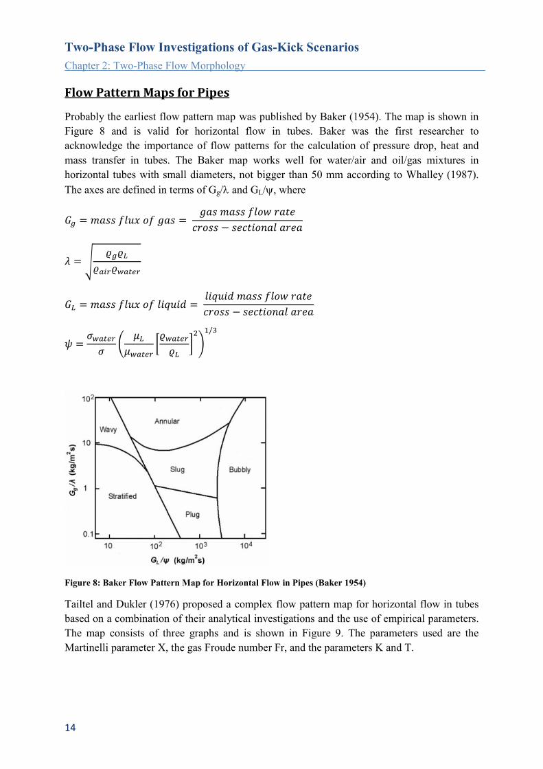
Flow Pattern Maps for Pipes
Probably the earliest flow pattern map was published by Baker (1954). The map is shown in
Figure 8 and is valid for horizontal flow in tubes. Baker was the first researcher to
acknowledge the importance of flow patterns for the calculation of pressure drop, heat and
mass transfer in tubes. The Baker map works well for water/air and oil/gas mixtures in
horizontal tubes with small diameters, not bigger than 50 mm according to Whalley (1987).
The axes are defined in terms of Gg/ and GL/, where
𝐺𝑔 = 𝑚𝑎𝑠𝑠 𝑓𝑙𝑢𝑥 𝑜𝑓 𝑔𝑎𝑠 = 𝑔𝑎𝑠 𝑚𝑎𝑠𝑠 𝑓𝑙𝑜𝑤 𝑟𝑎𝑡𝑒
𝑐𝑟𝑜𝑠𝑠 − 𝑠𝑒𝑐𝑡𝑖𝑜𝑛𝑎𝑙 𝑎𝑟𝑒𝑎
𝜆 = √𝜚𝑔𝜚𝐿
𝜚𝑎𝑖𝑟𝜚𝑤𝑎𝑡𝑒𝑟
𝐺𝐿 = 𝑚𝑎𝑠𝑠 𝑓𝑙𝑢𝑥 𝑜𝑓 𝑙𝑖𝑞𝑢𝑖𝑑 = 𝑙𝑖𝑞𝑢𝑖𝑑 𝑚𝑎𝑠𝑠 𝑓𝑙𝑜𝑤 𝑟𝑎𝑡𝑒
𝑐𝑟𝑜𝑠𝑠 − 𝑠𝑒𝑐𝑡𝑖𝑜𝑛𝑎𝑙 𝑎𝑟𝑒𝑎
𝜓 =𝜎𝑤𝑎𝑡𝑒𝑟
𝜎(
𝜇𝐿
𝜇𝑤𝑎𝑡𝑒𝑟[𝜚𝑤𝑎𝑡𝑒𝑟
𝜚𝐿]
2
)
1/3
Figure 8: Baker Flow Pattern Map for Horizontal Flow in Pipes (Baker 1954)
Tailtel and Dukler (1976) proposed a complex flow pattern map for horizontal flow in tubes
based on a combination of their analytical investigations and the use of empirical parameters.
The map consists of three graphs and is shown in Figure 9. The parameters used are the
Martinelli parameter X, the gas Froude number Fr, and the parameters K and T.

Two-Phase Flow Investigations of Gas-Kick Scenarios
Chapter 2: Two-Phase Flow Morphology
15
Figure 9: Two-phase Flow Pattern Map for
Horizontal Flow in Tubes (Taitel and Dukler 1976)
𝑋 = [(𝑑𝑝/𝑑𝑧)𝐿
(𝑑𝑝/𝑑𝑧)𝑔]
1/2
𝐹𝑟 =𝐺𝑔
[𝜚𝑔(𝜚𝐿 − 𝜚𝑔)𝑑𝑔]1/2
𝐾 = 𝐹𝑟 [𝐺𝐿𝑑
𝜇𝐿]
12
𝑇 = [|(𝑑𝑝/𝑑𝑧)𝐿|/𝑔(𝜚𝐿 − 𝜚𝑔)]1/2
The frictional pressure gradients (dp/dz) needed to compute the parameters, are either defined
for the liquid or the gas flowing alone in the tube of diameter d. To use the map one first
determines the Martinelli parameter and the gas-phase Froude number. Looking up the
coordinates in the first graph provides information, if an annular flow regime is present. In
case the coordinates fall into the other regions one determines the next parameter K, and
proceeds to the next graph and so on. A detailed explanation of this map can be found in
Whalley (1987).
The flow pattern map of Griffith and Wallis (1961) shown in Figure 10 provides a general
guide of flow patterns in vertical flow. Several flow patterns are grouped together, and only
three flow pattern groups are differentiated. It uses dimensionless ratios for the representation
of the flow patterns. Qg and Ql are the volumetric flowrates of the gas and liquid phases
respectively. A is the cross sectional area and d0 is the equivalent diameter. The vertical axis
indicates how much space is occupied by the gas phase and the horizontal axis indicates the
kinetic energy of the total flow.

Two-Phase Flow Investigations of Gas-Kick Scenarios
Chapter 2: Two-Phase Flow Morphology
16
Figure 10: Flow Pattern Map of Griffith and Wallis (1961)
For 2-phase flow in vertical tubes the flow pattern maps of Fair (1960) and Hewitt and
Roberts (1969) are still among the most widely quoted maps. Figure 11 shows the flow
pattern map of Fair (1960), it is based on the overall mass velocity on the vertical axis and a
parameter combining the information on vapor quality x, viscosity and density ratio of gas
and liquid on the horizontal axis.
Figure 11: Two-phase Flow Pattern Map for Vertical Tubes, Fair (1960)
The flow pattern map introduced by Hewitt and Roberts in 1969 is shown in Figure 12. This
is an empirical flow pattern map describing the flow patterns for co-current upward flow in a
vertical pipe. Hewitt and Roberts correlated both air/water data at atmospheric pressure and
steam/water flow at high pressure. The map is based on the gas and liquid superficial
momentum flux rather than volumetric or mass fluxes, and is valid for a wide range of flow
rates.

Two-Phase Flow Investigations of Gas-Kick Scenarios
Chapter 2: Two-Phase Flow Morphology
17
Figure 12: Hewitt and Roberts Flow Pattern Map for Vertical Upward Flow in a Pipe (Whalley, 1987)
In contrast to empirical flow pattern maps mechanistic flow pattern maps are based on
fundamental considerations and identification of dominant forces found through examination
of various flow transition phenomena. These types of maps cover a wider range of
experimental conditions than the empirical ones due to having incorporated system
parameters. Taitel et al. (1980) presented an alternative to the experimental methods of
obtaining flow pattern maps. They considered the conditions necessary for the existence of
each of the flow patterns and postulated mechanisms by which the transitions between the
various flow patterns might occur. The widely applied models by Taitel et al. (1980), Jayanti
and Hewitt (1992) and Barnea (1986) describe the bubble to-slug, slug-to-churn and churn-to-
annular flow transitions. Jayanti and Hewitt (1992) improved the modeling of the flooding
mechanism given by McQuillan and Whalley (1985) which is dominating the transition from
slug to churn flow. At the onset of churn flow a sharp increase in pressure gradient can be
observed, this was investigated and reported by Owen (1986). The differentiation of flow
patterns based on his results is illustrated in Figure 13.

Two-Phase Flow Investigations of Gas-Kick Scenarios
Chapter 2: Two-Phase Flow Morphology
18
Figure 13: Pressure Gradient Data of Fully Developed Air-water Flow in a Vertical Tube, Owen (1986)
Barnea (1987) mentions a unified model for flow pattern transitions for the whole range of
pipe inclinations. His work especially focused on the transition from annular to intermittent
flows. According to literature the most widely recommended flow pattern maps for vertical
tubes are those of Barnea et al. (1987), Fair (1960), Hewitt and Robertson (1969), and Chen et
al. (2006).
Flow Patterns in Annular Geometries
In the literature only few studies can be found on flow patterns in annular flow geometries.
One of them is the work done by Caetano et al. (1992), who conducted experimental and
theoretical studies on gas-liquid flow through an annulus. Their studies covered vertical
upward flow in both concentric and fully eccentric annuli. Air-water and air-kerosene
mixtures were used as flowing fluids. Their analysis revealed that application of the hydraulic
diameter concept as a characteristic dimension for annuli configurations is not always
adequate, especially for small Reynolds number flows. When studying Taylor bubble rise
velocity they observed bubble velocity to rise at a faster velocity as the pipe diameter ratio
increases. The shape of the Taylor bubbles in the annuli configuration showed no spherical
cap or rotational symmetry as it does in pipes. The presence of the inner pipe causes a
deformation of the Taylor bubbles as if it is cutting through the bubble. Additionally there
appears a channel through the torus bubble body where the fluid is flowing backwards.
The work of Caetano presents flow pattern definitions and experimental flow pattern maps for
annuli configurations, based on a modification of Taitel et al. (1980) model for flow pattern
transitions in pipe flow. Figure 14 and Figure 15 show the flow patterns occurring in
concentric and eccentric annuli. The same flow patterns can be found as in pipe flow,
however with substantially different characteristics.

Two-Phase Flow Investigations of Gas-Kick Scenarios
Chapter 2: Two-Phase Flow Morphology
19
Figure 14: Flow Pattern in Upward Vertical Flow
Through a Concentric Annulus, taken from
Caetano et al. (1992)
Figure 15: Flow Pattern in Upward Vertical Flow
Through a Fully Eccentric Annulus, taken from
Caetano et al. (1992)
Figure 16 shows a flow pattern map based on the studies of Caetano et al. (1992).
Figure 16: Flow Pattern Map for Upward Two-phase Flow in Annulus after Caetano et al. (1992)

Two-Phase Flow Investigations of Gas-Kick Scenarios
Chapter 2: Two-Phase Flow Morphology
20
Conclusion on Flow Pattern Maps
Flow pattern maps and transition criteria are developed from experiments and carried out for
steady-state, fully developed flows. Taitel et al. (1980) discussed the various flow pattern map
parameters available, and argued that the various flow pattern transitions cannot all be
represented by any given coordinate pair. The flow pattern depends on multiple
dimensions/parameters containing the physical properties of the phases as well as the
geometric configuration of the flow domain. Another basic issue regarding flow pattern maps
is that they are often dimensional and therefore apply only to a specific two-phase flow setup.
Some flow pattern maps attempt to take account of channel geometry and fluid physical
properties by suitable adaptation of the parameters which are plotted. A number of
investigators (for example Baker 1954, Schicht 1969, Weisman and Kang 1981) have
attempted to find generalized coordinates that would allow the map to cover different fluids
and pipes of different sizes. Brennen (2005) pointed out that such generalizations are only of
limited value because several transitions are represented in most flow pattern maps and the
corresponding instabilities are governed by different sets of fluid properties. For example, one
transition might occur at a critical Weber number, whereas another boundary may be
characterized by a particular Reynolds number. Macroscopic parameters like superficial
velocities and flow rates of the phases alone are often not sufficient to characterize the flow
pattern because they are missing essential information. Even the assumption that there exists a
unique flow pattern for given fluids with given flow rates is not correct. Hewitt and Hall-
Taylor (1972) found out that one of the most important variables in determining the flow
pattern is the manner in which the phases are introduced into the channel. Similarly, Brennen
(2005) showed that even very simple models of multiphase flow can lead to conjugate states.
Naturally there could be several possible flow patterns at certain flow conditions only
depending on the initial condition i.e. how the multiphase flow was initiated. This fact is often
completely ignored. A certain flow pattern is in fact a function of multiple parameters and can
therefore only be coarsely described in 2-dimensional flow pattern map.
In general flow patterns depend on:
Gas and liquid fluid properties (i.e. density, viscosity, etc.)
Operational parameters (i.e. pressure, temperature, flow rates and direction, inclination
angle, etc.)
Flow channel geometry (i.e. cross sectional area, diameter, annular clearance,
eccentricity, etc.)
Inlet condition (i.e. geometric inlet configuration, inlet boundary condition)
As a consequence there exists no universal, dimensionless flow pattern map that incorporates
the full parametric dependence of the flow pattern on the fluid characteristics, boundaries and
initial conditions. One has to be aware, that the concept of flow patterns is merely qualitative
and subjective.
Two-Phase Flow Investigations of Gas-Kick Scenarios
Chapter 3: Two-Phase Flow Modeling
21
3. Two-Phase Flow Modeling
Basically one can investigate and model two-phase flow experimentally and/or theoretically.
In petroleum engineering the most common task in modeling two-phase flow in pipe or
annular geometries is the identification of a flow-pattern map. The identification of flow
patterns has historically been used to assess the success of drilling and production, since the
morphology of the flow determines physical phenomena like mass and heat exchange,
mechanical wear and pressure drop. Regarding the two-phase flow situation of a gas-kick the
ability to set up an experimental model is very limited and costly. Due to the hazardous nature
of H2S and high pressure conditions needed to reproduce bottom-hole conditions, large-scale
experiments can hardly be found in literature. It is more common to conduct sour gas
experiments in an autoclave or other small volume test apparatus to gain information for the
characterization of reactions and by-products in the corrosion process. However such an
approach lacks the mechanical impact of the flow pattern on the corrosion process. Especially
the slug flow pattern is assumed to cause an increase in corrosion rate, due to the removal of
protective scales by the flow fluctuations. So as a consequence of the extreme dimensions and
pressure conditions this flow problem demands for a reliable theoretical or computational
model instead.
The mathematical description and its physical model for numerical computation can be done
on different levels of sophistication according to the degree of information needed and the
means available. For the mathematical and physical description of two-phase flow one may
consider the flow field to be composed by single-phase regions with moving boundaries in
between. The difficulties in modeling two-phase flow arise from the unsteady nature of this
boundary and its influence on the flow field. Additionally processes like heat and mass
transfer at the phase interface increase the set of equations that need to be solved. Modelling
the detailed distribution of the interfaces in time and space for any particular flow is clearly
impossible. Instead simplifications according to the degree of information needed are
required.
The goal of this work is to investigate and analyze gas-liquid flow in great detail. To achieve
this, computational modeling appears to be the most appropriate choice. The next sections
will give a general overview on the governing forces and modeling approaches in two-phase
flow.

Two-Phase Flow Investigations of Gas-Kick Scenarios
Chapter 3: Two-Phase Flow Modeling
22
Navier-Stokes Equations
The fundamental continuum mechanics equations to describe the motion of fluids are the
Navier-Stokes equations. These equations are a set of equations that contain the conservation
laws for mass, momentum and energy for a single phase.
Looking at single phase flow we know that any movement of a fluid is caused by forces
acting on the fluid element. Basically these forces can be grouped into three categories
according to their proportionality to dimensions in space, i.e. volume forces, surface forces,
and line forces.
Table 1: Forces acting on a fluid element
Volume Forces Surface Forces Line Forces
Gravity force
Inertia force
Buoyancy force
Pressure force
Viscous force
Surface tension force
Regarding the fluid as a continuum and applying Newton’s second law of motion combined
with the assumption that the stress state in the fluid is made up by a pressure term and a
viscous term, one derives the equation of motion for a fluid element:
𝜌𝑑˅
𝑑𝑡= ∇ ∙ 𝜎 + 𝐹
where is the stress tensor, and F accounts for body forces present.
This equation basically states the conservation of momentum, i.e. the sum of all forces acting
on a fluid element is equal to its temporal change in momentum. The change in flow,
acceleration or deceleration of the fluid element is dependent upon the force exerted on it and
is proportional to its mass. This is the property of conservation of momentum and is simply
Newton’s second law.
The time-derivative of the fluid velocity is defined as:
𝑑˅
𝑑𝑡=
𝜕˅
𝜕𝑡+ ˅ ∙ ∇˅
The stress tensor can be split up into two terms, the pressure p times the identity matrix I and
the deviatoric stress tensor T.
𝜎𝑖𝑗 = (
𝜎𝑥𝑥 𝜏𝑥𝑦 𝜏𝑥𝑧
𝜏𝑦𝑥 𝜎𝑦𝑦 𝜏𝑦𝑧
𝜏𝑦𝑧 𝜏𝑧𝑦 𝜎𝑧𝑧
) = − (
𝑝 0 00 𝑝 00 0 𝑝
) + (
𝜎𝑥𝑥 + 𝑝 𝜏𝑥𝑦 𝜏𝑥𝑧
𝜏𝑦𝑥 𝜎𝑦𝑦 + 𝑝 𝜏𝑦𝑧
𝜏𝑦𝑧 𝜏𝑧𝑦 𝜎𝑧𝑧 + 𝑝) = −𝑝Ι + Τ
Updating the equation of motion gives the following general form:

Two-Phase Flow Investigations of Gas-Kick Scenarios
Chapter 3: Two-Phase Flow Modeling
23
𝜌𝑑˅
𝑑𝑡= −∇𝑝 + ∇Τ + 𝐹
This equation is still needs information about the unknown stress tensor T. A constitutive law
is needed describing the viscous stress state in the fluid. This constitutive law describes the
viscous behavior or rheology of the fluid. In case of Newtonian fluids, there is a linear
relationship between applied stress and resulting strain, so fluid viscosity is a constant,
applying this relationship leads to:
Τ𝑖𝑗 = 𝜇 (𝜕𝑢𝑖
𝜕𝑥𝑗+
𝜕𝑢𝑗
𝜕𝑥𝑖) + 𝛿𝑖𝑗𝜆∇ ∙ ˅
were δij is the Kronecker delta, μ and λ are proportionality constants associated with the
assumption that stress depends on strain linearly, μ is called the first coefficient of viscosity
and λ is the second coefficient of viscosity. The value of λ, which produces a viscous effect
associated with volume change, is very difficult to determine, the most common
approximation is λ ≈ - ⅔ μ.
Substitution of Tij yields the equation of motion for a Newtonian fluid:
𝜌 (𝜕˅
𝜕𝑡+ ˅ ∙ ∇˅) = −∇𝑝 + ∇ ∙ (𝜇(∇˅ + (∇˅)𝑇) −
2
3𝜇(∇ ∙ ˅)Ι) + 𝜌𝑔
with gravity applied as external force. If one wants to account for the surface tension force at
the phase interface in two-phase flow, then exact knowledge about the phase interface is
needed. The treatment of the phase interface will be discussed in a later chapter.
The equation of motion can also be expressed in the following terms:
𝐼𝑛𝑒𝑟𝑡𝑖𝑎𝑙 𝑓𝑜𝑟𝑐𝑒𝑠 = 𝑝𝑟𝑒𝑠𝑠𝑢𝑟𝑒 𝑓𝑜𝑟𝑐𝑒𝑠 + 𝑣𝑖𝑠𝑐𝑜𝑢𝑠 𝑓𝑜𝑟𝑐𝑒𝑠 + 𝑒𝑥𝑡𝑒𝑟𝑛𝑎𝑙 𝑓𝑜𝑟𝑐𝑒𝑠
Additionally the continuity principle imposes that mass is conserved unless it passes out of
the domain. The conservation of mass, without any sources or sinks, is defined as:
𝜕𝜌
𝜕𝑡+ ∇ ∙ 𝜌˅ = 0
Compressible flow additionally requires an equation of state and the conservation of energy
formulation. The ideals gas law is often used as an equation of state, but basically the
relationship to be used depends on the fluid and the operating conditions.
Conservation of energy is defined as:
𝜌𝑑ℎ
𝑑𝑡=
𝑑𝑝
𝑑𝑡+ ∇ ∙ (𝑘∇𝑇) + Φ
where h is the enthalpy, k is a heat conduction coefficient, T is the temperature, and Φ is a
function representing the dissipation of energy due to viscous effects.

Two-Phase Flow Investigations of Gas-Kick Scenarios
Chapter 3: Two-Phase Flow Modeling
24
This set of three equations is termed the Navier-Stokes equations, which build the heart of
fluid flow modeling. Once the velocity field is calculated, other quantities of interest, such
as pressure or temperature, may be found. For certain flow situation simplifications can be
made allowing an analytical solution of the set of equations. Nevertheless the full Navier-
Stokes equations can only be solved numerically. The Navier-Stokes equations can describe
the motion of every phase in every detail, i.e. in every drop or bubble and surrounding fluid
when resolving the whole range of spatial and temporal scales. But the computer power
required to do this, which is called a direct numerical simulation, is far beyond present
capability for most of the flows that are commonly experienced.
The Navier-Stokes equations can be applied to each phase up to an interface but not across it.
Special treatment is needed at the interface to account for the sharp changes in variables and
to specify the exchange of mass, momentum and energy between the phases. A multitude of
different approaches have been put forward to cover the wide spectrum of multiphase flow of
different scales. These approaches basically involve the solution of the Navier-Stokes
equations combined with additional flow specific models and assumptions. When one or both
of the phases becomes turbulent the computational challenge can become enormous.
Therefore, simplifications are essential in realistic models of most multiphase flows.
Reasonable simplifications of the governing equations can only be based on a clear
understanding of the flow and investigation of the dominant forces and mechanisms.
Traditionally an engineer starts the characterization of the flow under investigation by the
means of dimensionless numbers.

Two-Phase Flow Investigations of Gas-Kick Scenarios
Chapter 3: Two-Phase Flow Modeling
25
Dimensionless Numbers
When looking at the forces in multiphase flow (Table 1) and their magnitude, the governing
forces are pressure force, inertia force, gravity force, buoyancy force, viscous force and surface
tension force. Naturally, all these forces are covered in the Navier-Stokes equations. When
formulating the forces individually and putting them into relation, non-dimensional groups can be
derived. These groups are referred to as dimensionless numbers in fluid mechanics. With these
numbers flow problems can be categorized and more important dominant forces are identified.
For many decades this approach was used to introduce simplifications in flow modeling. Before
setting up a computational model, it is still good engineering practice to analyse the flow
problem by assessing its dominant forces and their key basic relations. This provides the basis
for a sound modeling approach and is often forgotten, as computational modeling tools and
computational power become more and more easily available. This section summarizes the
definition and importance of dimensionless numbers in fluid mechanics relevant to multiphase
flow.
Based on the six fundamental forces in fluid mechanics the following five independent
dimensionless groups can be derived. A detailed explanation and the corresponding equations
are given subsequently.
Table 2: Dimensionless Groups in Fluid Mechanics
Re Reynolds number 𝒊𝒏𝒕𝒆𝒓𝒊𝒂 𝒇𝒐𝒓𝒄𝒆
𝒗𝒊𝒔𝒄𝒐𝒖𝒔 𝒇𝒐𝒓𝒄𝒆
Eu Euler number 𝒑𝒓𝒆𝒔𝒔𝒖𝒓𝒆 𝒇𝒐𝒓𝒄𝒆
𝒊𝒏𝒆𝒓𝒕𝒊𝒂 𝒇𝒐𝒓𝒄𝒆
Fr Foude number 𝒊𝒏𝒕𝒆𝒓𝒊𝒂 𝒇𝒐𝒓𝒄𝒆
𝒇𝒐𝒓𝒄𝒆 𝒐𝒇 𝒈𝒓𝒂𝒗𝒊𝒕𝒚
We Weber number 𝒊𝒏𝒕𝒆𝒓𝒊𝒂 𝒇𝒐𝒓𝒄𝒆
𝒔𝒖𝒓𝒇𝒂𝒄𝒆 𝒕𝒆𝒏𝒔𝒊𝒐𝒏 𝒇𝒐𝒓𝒄𝒆
Eo Eötvös number 𝒃𝒖𝒐𝒂𝒏𝒄𝒚 𝒇𝒐𝒓𝒄𝒆
𝒔𝒖𝒓𝒇𝒂𝒄𝒆 𝒕𝒆𝒏𝒔𝒊𝒐𝒏 𝒇𝒐𝒓𝒄𝒆
The first three of them are well known from single phase flow, but do also play an important role
in the characterization of multiphase flow. More dimensionless numbers apart from the ones listed
in Table 2 can be found in literature. But basically they can be derived by rearranging the five
fundamental groups. For instance Archimedes number (Ar), Capillary number (Ca), inverse
viscosity number (Nf), Morton number (Mo), Ohnesorge number (Oh), and Suratman number (Su)
can be derived by combining two or more dimensionless numbers as follows:
𝐴𝑟 = √1
𝑀𝑜 = 𝑅𝑖 ∙ 𝑅𝑒2, 𝐶𝑎 =
𝐹𝑟
√𝑀𝑜𝐸𝑜4 =
𝑊𝑒
𝑅𝑒 , 𝑁𝑓 = √
𝐸𝑜3
𝑀𝑜
4
,
Two-Phase Flow Investigations of Gas-Kick Scenarios
Chapter 3: Two-Phase Flow Modeling
26
𝑀𝑜 =𝐸𝑜𝑊𝑒2
𝑅𝑒4 , 𝑂ℎ =
√𝑊𝑒
𝑅𝑒 , 𝑆𝑢 =
𝑅𝑒²
𝑊𝑒
The most popular dimensionless number in fluid dynamics is probably the Reynolds number. It
represents the ratio between inertia and viscous forces, or in other words relates the fluids
momentum to its viscosity. It is primarily used to characterize single phase flow as either
turbulent or laminar.
𝑅𝑒 =𝐹𝐼
𝐹𝑉
=𝜌𝐿𝑈
𝜇
ρ fluid density L characteristic length, i.e. hydraulic radius U mean velocity of the fluid
dynamic fluid viscosity
Multiphase flows are usually considered turbulent, although laminar flow can occur when the
flow channel or conduit is aligned horizontal. In inclined flows buoyancy is affecting the flow
causing the lighter phase to accelerate and generate turbulences. Naturally in multiphase flow the
concept of the Reynolds number needs to be revised. One approach is to use mixture quantities to
compute a mixture Reynolds number. This approach might be valid in case of dispersed flow with
low slip velocity. But in case of segregated flow, where fluid velocities differ considerably, this
approach is not sufficient to describe the flow situation. In this case the Reynolds number should
rather be computed for each phase using the individual phase velocities and properties. However
there is no general consensus on what to use for an appropriate definition of Reynolds number for
multiphase flow. It is up to the researcher to select a definition that best describes the flow under
investigation.
The Euler number represents the ratio between pressure forces and inertia forces. It relates a
local pressure gradient to the kinetic energy of the fluid volume. It is used to characterize losses in
the flow and is defined as:
𝐸𝑢 =𝐹𝑃
𝐹𝐼
=∆𝑝
𝜌𝑈2
Δp pressure gradient
A perfect frictionless flow corresponds to an Euler number of 1.
The Froude number describes different flow regimes of open channel flow. It is defined as the
ratio of the flow inertia and gravity:
𝐹𝑟 =𝐹𝐼
𝐹𝐺
= √𝜌𝑈2
2𝜌𝑔ℎ
=𝑈
√𝑔𝐿
g acceleration due to gravitation h hydraulic depth L characteristic length, i.e. height of the liquid film

Two-Phase Flow Investigations of Gas-Kick Scenarios
Chapter 3: Two-Phase Flow Modeling
27
The Froude number is of importance whenever there is a fluid flow with a free interface. This is
certainly true in separated two-phase flow. For this type of flows the Froude number seems a good
correlating parameter. Flows with the same Froude number have similar wave patterns at the
phase interface. The denominator represents the speed of a small surface wave relative to the
speed of the bulk fluid, called wave celerity. Based on the Froude number open channel flow is
classified into three types:
Fr = 1, critical flow Fr > 1, supercritical flow Fr < 1, subcritical flow
At critical flow wave celerity equals bulk flow velocity. Any disturbance to the flow will
remain stationary. In subcritical flow the bulk flow velocity is slower than the wave velocity
and hence flow disturbances are transmitted upstream and downstream. This condition leads
to backwater effects. In supercritical flow the bulk flow is faster than the surface wave
causing disturbances to be transmitted only downstream. It is only in supercritical flows that
hydraulic jumps can occur.
The above definition of the Froude number and of flow classification is only valid for free
surface, i.e. flows in horizontal channels with the denser fluid flowing at the bottom. Several
extensions of the Froude number exist to cover effects like inclination (pressure potential and
gravity potential), fluid rotation, and buoyancy (Densimetric Froude number).
The relevance of the Froude number to characterize gas-liquid flow in pipes can be seen in the
work of Taha and Cui (2005). Their work presents a numerical study investigating the motion of a
single Taylor bubble. Based on a dimensional analysis the following definition of the Froude
number, as the ratio between inertia and buoyancy forces, is used:
𝐹𝑟𝑔𝑎𝑠 =𝑈𝑇𝐵
√𝑔𝑑𝜌𝑙 − 𝜌𝑔
𝜌𝑙
UTB Taylor bubble velocity ρg gas density ρl liquid density d pipe diameter
The publication of Taha and Cui (2005) contains a good literature overview on previous work
done regarding dimensionless groups to characterize slug flow. Their study of single Taylor
bubble movement in stagnant and flowing liquid is a good basis to understand the complicated
nature of slug flow.
The Weber number represents the ratio of inertia force to surface tension force.
𝑊𝑒 = 𝐹𝐼
𝐹𝑆
=𝜌𝐿𝑈²
𝜎
surface tension

Two-Phase Flow Investigations of Gas-Kick Scenarios
Chapter 3: Two-Phase Flow Modeling
28
Inertia is the driving force causing partial disruption of flow structures and is counteracted by
the resistance due to interfacial tension. Increased Weber numbers are associated with a
greater tendency for droplet deformation and breakup to occur at higher shear, i.e. with more
intense mixing. The Weber number is useful for the determination of stable bubble diameters
and bubble distortion tendency under certain flow conditions. When surface tension forces are
dominant, the bubble tends to be spherical and when inertial forces are dominant, the bubble
tends to have a hemispherical shape.
The Eötvös number, also called Bond number, represents the relative significance of
buoyancy and surface tension.
𝐸𝑜 = 𝐵𝑜 =𝐹𝐵
𝐹𝑆
=(𝜌𝑙−𝜌𝑔)𝑔𝑑²
𝜎
A small Eötvös number indicates a strong influence of surface tension resulting in a rather
spherical bubble shape whereas a large Eötvös number results in distorted bubble shapes and
increased bubble velocity. The Eötvös number is often used in combination with the Morton
number to characterize bubble and droplet shapes.
In multiphase flow, forces like the surface tension force can have a significant effect on the flow
morphology and hence need to be considered. Based on the assumption that the inertia and
viscous forces in the gas are much smaller than those in the liquid a group of three dimensionless
numbers is well suited to cover the relationship of relevant forces. Typical groups of
dimensionless numbers so characterize gas-liquid flow that are frequently found in literature are:
Froude & Morton & Eötvös number
Froude & Eötvös & Nf number
Froude & Nf & Archimedes number
An example for the use of the first dimensionless group is shown in Figure 17, representing the
correlation of experimental data on the rise of Taylor bubbles obtained by White and Beardmore
(1962). Taylor bubbles were observed in vertical tubes rising through several different stagnant
fluids. The Morton number shown in the graph represents the fluid properties, the Froude number
represents the bubble rising velocity and the Eötvös number illustrates the influence of surface
tension. For certain Morton numbers bubbles may not even rise below a critical Eötvös number.
There is a region for Eo < 70 where the Froude number i.e. rising velocity is a function of Eötvös
number only. At Eo > 200 there is an inertial region where liquid viscosity and surface tension
are less important.

Two-Phase Flow Investigations of Gas-Kick Scenarios
Chapter 3: Two-Phase Flow Modeling
29
Figure 17: Correlation of the Rise Velocity of Cylindrical Bubbles (White & Beardmore 1962)
The inverse viscosity dimensionless number Nf represents the influence of liquid viscosity and
geometry on phase mixing in slug flow.
𝑁𝑓 =√𝑔𝑑3
𝜈𝑙
𝜈𝑙 kinematic viscosity of liquid
Guedes de Carvalho (1988) used the inverse viscosity number to classify the wake behind Taylor
bubbles. They identified three different patterns, i.e a closed axisymmetric wake for Nf <500,
closed unaxisymmetric wake for 500<Nf<1500 and opened wake with recirculatory flow for
Nf>1500. Their experimental results were simulated by Taha and Cui (2005) and matched
favorably as shown in Figure 18.

Two-Phase Flow Investigations of Gas-Kick Scenarios
Chapter 3: Two-Phase Flow Modeling
30
0,066 0,064 0,064 0,063 0,064 Eo
0,30 0,341 0,351 0,351 0,341 Fr
84 176 205 325 1528 Nf
Figure 18: Wake Flow Pattern at Different Values of Nf, taken from Taha and Cui (2005)
Extending the inverse viscosity number with the fluid densities one derives the buoyancy
Reynolds number R, defined as
𝑅 =√𝑔𝑑3(𝜌𝑙 − 𝜌𝑔)𝜌𝑙
𝜇𝑙
Viana et al. (2003) gathered extensive experimental data on the rise velocity of Taylor bubbles in
stagnant fluids for their universal correlation approach. They used a group of dimensionless
velocity, buoyancy Reynolds number, and Eötvös number to characterize the flow. Figure 19
illustrates the shape of the wake behind the Taylor bubble in dependence of dimensionless
numbers, R and Eo respectively. With decreasing viscosity the perfect shape of the bubble gets
more and more distorted until eventually a highly turbulent region with small bubbles forms in the
wake.

Two-Phase Flow Investigations of Gas-Kick Scenarios
Chapter 3: Two-Phase Flow Modeling
31
Figure 19: Taylor Bubble Wake Morphology according to Buoyancy Reynolds Number, taken from Viana
et al. (2003)
The Morton number is defined as
𝑀𝑜 =𝐹𝐵𝐹𝑉
4
𝐹𝐼2𝐹𝑆
3 =𝑔(𝜌𝑙 − 𝜌𝑔)𝜇𝑙
4
𝜌𝑙2𝜎3
l dynamic viscosity of liquid
The Morton number is used to characterize dispersed two phase flows. It is only dependent on
fluid properties and is sometimes referred to as the property group. At atmospheric pressure the
density of gas is often neglected in the definition of the number. The Morton number relates
viscous forces to surface tension forces. According to the Morton number fluids can be arranged
into two groups, those with high Morton numbers (Mo > 10-2) and those with low Morton
numbers (Mo < 10-6). Water for instance has a Morton number of 1.1e-11. High viscosity
drilling fluids typically show high Morton numbers.
Ohnesorge Number relates the viscous forces to inertial and surface tension forces.
𝑂ℎ =𝐹𝑉
√𝐹𝐼𝐹𝑆
=𝜇
√𝜌𝜎𝐿
The combination of these three forces into one masks the individual effects of every force. It
is used in spray technology to describe bubble and droplet distortion. Larger Ohnesorge
numbers indicate a greater effect of the viscosity.
Two-Phase Flow Investigations of Gas-Kick Scenarios
Chapter 3: Two-Phase Flow Modeling
32
Suratman number, also known as Laplace number, is used for characterization of free surface
flows. It is defined as the ratio of surface tension to momentum-transport:
𝑆𝑢 = 𝜌𝑙𝑑𝜎
𝜇𝑙2 =
𝑅𝑒²
𝑊𝑒
This number depends only on the properties of the liquid and the pipe diameter, and does not
depend on the flow rates of the liquid or gas. It is used in some flow pattern maps to account
for channel geometry and fluid properties.
Richardson number describes the ratio of potential to kinetic energy.
𝑅𝑖 = 𝐸𝑝
𝐸𝑘
There are several variants of the Richardson number. In general it is an essential parameter
describing turbulence of sheared stratified flows. The Richardson number indicates the onset of
the Kelvin Helmholtz instability. An instability that arises in parallel shear flows, where small-
scale perturbations draw kinetic energy from the mean flow. A typical example is the formation,
rise, and braking of waves. Another important fluid dynamic phenomenon is the Rayleigh-Taylor
instability. This instability describes the distortion of an interface between two fluids of
different density which occurs when the lighter fluid is pushing the heavier fluid.
Some other important dimensionless numbers of relevance when dealing with mass transfer in
two-phase flow are the Sherwood number and the Schmidt number.
The Sherwood number is the dimensionless form of the mass transfer coefficient. It is defined as
the ratio of
𝑆ℎ =𝑘𝐿
𝐷
k mass transfer coefficient L characteristic length scale D mass diffusivity
Schmidt number relates the diffusivity of momentum to the diffusivity of mass:
𝑆𝑐 =𝜈
𝐷
𝜈 kinematic viscosity D diffusivity
The Schmidt number plays a role in mass transfer. It relates the molecular ability of a fluid to
transport momentum to its ability to transport species. The Schmidt number of gases is
typically in the order of unity. In liquids where molecules are packed closely together
diffusion is much slower but momentum is efficiently transmitted through molecular
interactions. Therefore, Schmidt numbers in liquids are typically three orders of magnitude
larger than those in gases.

Two-Phase Flow Investigations of Gas-Kick Scenarios
Chapter 3: Two-Phase Flow Modeling
33
Dimensional Analysis
Although some of the fluid flow relevant forces can be neglected in certain cases, it is a
challenging task to determine which one is dominant at specific conditions. The sensible selection
of relevant forces can provide great benefits in the subsequent modeling effort. Such
simplification of the problem can lead to even analytical solutions of the Navier-Stokes equation;
see literature on Hagen-Poiseuille flow or Couette flow as an example.
Dimensional analysis is the mathematical tool to assess the relation of physical quantities
without knowing an exact formulation of the problem at hand. This approach has been well
applied in fluid dynamics to realize geometrically similar experimental setups or simplified
computational models representing a far more complex flow problem at first. Dimensional
analysis is the basis for similitude theory. Physicians like Ludwig Prandtl, Theodore von
Karman, Johann Nikuradse and many others used this theory at the end of the 19th
century to
reproduce flows of different length scales in their lab experiments by altering fluid viscosity
and density.
The prior task in dimensional analysis is to highlight the dominant forces, their relevant
relations and effects in the physical system under investigation. This information is best
summarized via dimensionless numbers. There are basically two approaches to identify the
relevant dimensionless numbers of a fluid-flow problem, either by applying the Π-Theorem,
or by reformulation of the governing equations so that they only contain dimensionless
variables.
The first approach will be shortly addressed in the next section. However, it has to be
recognized that the dimensional analysis provides answer to what group of parameters affect
the problem and not the answer to the problem.
Π-Theorem
The Buckingham Π-Theory requires no knowledge about the underlying equations. Due to its
simplicity this approach may sometimes yield insufficient knowledge, but the method has its
usefulness when no governing equations are found. In this technique only the dimensions or
the properties of the problem at hand are analyzed.
The basic set of seven dimensions that can describe any physical problem consists of length,
mass, time, electric current, temperature, luminous intensity, and quantity of substance. These
dimensions can be recombined to create derived dimensions, like for instance velocity,
acceleration, density, viscosity and so on. When describing a fluid mechanics problem a
reduced set of fundamental dimensions is usually sufficient. The choice of whether to use
fundamental dimensions or derived dimensions is not unique it is only a matter of preference.
For example, one could use the combination of mass, time, length or instead force, time,
length.

Two-Phase Flow Investigations of Gas-Kick Scenarios
Chapter 3: Two-Phase Flow Modeling
34
The following five out of the seven afore mentioned fundamental dimensions are relevant in
the description of multiphase flow including mass transfer:
Length (L)
Mass (M)
Time (θ)
Temperature (T)
Quantity of substance (N)
They build the basis to describe all physical phenomena occurring during a gas-kick in a
wellbore. The number of basic dimensions a problem has determines the number of the
combinations which affect the physical situations. The total number of dimensions, i.e. the
sum of fundamental and derived dimensions, a problem has can therefore be reduced because
these dimensions are repeating or reoccurring.
The Buckingham method is based on the fact that all equations must be consistent with their
units and that they can be divided to create dimensionless equations. The terms in the
equations are then dimensionless parameters or also termed Π-Factors. This idea leads to the
assumption that these dimensionless parameters can be found without any knowledge of the
governing equations.
The analysis starts with the preparation of a list of parameters that are presumed to define the
behavior of interest. Considering a gas-kick in a wellbore and its fluid dynamic effect on drill-
pipe corrosion, the following list of parameter is assumed to define the flow system:
ULS Superficial mud velocity UGS Superficial gas velocity
l Mud density
g Gas density
µl Mud viscosity µg Gas viscosity
Surface tension d Annular clearance g gravity CH2S Concentration of dissolved H2S k Mass transfer coefficient D Molecular diffusion coefficient S Gas solubility
This list is valid for fully developed flow and restricted to a limited section of the wellbore.
No entrance effects are considered. This is expressed by the independence on time and an
absence of a z-coordinate. Gas phase density is based on bottom-hole pressure and assumed to
stay constant in this section.
The corrosive threat caused by the flow can be expressed as the following functional
dependence:
𝑐𝑜𝑟𝑟𝑜𝑠𝑖𝑣𝑒 𝑡ℎ𝑟𝑒𝑎𝑡 = f 𝑈𝐿𝑆, 𝑈𝐺𝑆, 𝜌𝑙, 𝜌
𝑔, 𝜇
𝑙, 𝜇
𝑔, 𝜎, 𝑑, 𝑔, 𝐶𝐻2𝑆, 𝑘, 𝐷, 𝑆

Two-Phase Flow Investigations of Gas-Kick Scenarios
Chapter 3: Two-Phase Flow Modeling
35
The term corrosive threat is used because the actual corrosive attack depends on far more
variables than only the presence of dissolved H2S and the flow conditions. The corrosive
attack itself is not subject of this investigation. Corrosive threat is used as an arbitrary
expression and is neither given an exact definition nor units. It is a theoretical contribution of
the 2-phase flow to the corrosion of the drill-pipe.
The main factors of contribution are the concentration of dissolved H2S and flow induced
erosion. The fluid-mechanical erosion of the drill pipe, protective coatings, and corrosive
products is caused by the flow field next to the pipe wall. This flow field exerts pressure and
viscous forces on the drill pipe surface. At a local scale of observation these forces are
dependent upon the drill pipe roughness, the fluid density and the local instantaneous fluid
velocity only. However for the dimensional analysis the flow field cannot be described at such
a high temporal and spatial resolution, instead macroscopic flow variables with respect to
time and space are needed. For instance the fluid mechanical damage of the drill pipe can
more abstractly be explained by transient pressure fluctuations as a function of two-phase
flow pattern and an assumption of single phase flow adjacent to the drill pipe surface exerting
an abrasive shear stress. Or even coarser by replacing the single phase wall shear stress with
the phase kinetic energy based on the superficial fluid velocities. The occurrence of transient
pressure fluctuations is dependent on the two-phase flow pattern in the channel. As discussed
earlier two-phase flow patterns are a function of multiple flow variables and can probably best
described with the aid of dimensionless groups.
The minimum number of independent dimensionless groups i required to describe the
fundamental behavior is defined as:
𝑖 = 𝑛 − 𝑚
where n is the number of variables and m is the number of fundamental dimensions.
For the current problem the number of variables is 13 and five fundamental units. Using the
Buckingham Pi theorem, this yields 13 – 5 = 8 independent dimensionless parameters.
The selection of a dimensionless group is arbitrary and there are different methods to
determine the set of dimensionless groups. Common methods are the method of combination,
the algebraic method, and the method of speculative reduction.

Two-Phase Flow Investigations of Gas-Kick Scenarios
Chapter 3: Two-Phase Flow Modeling
36
The next step is to prepare a matrix of the variable’s dimensions. Based on the problem at
hand the resulting matrix reads:
ULS UGS l g µl µg d g CH2S k D S
L 1 1 -3 -3 -1 -1 0 1 1 -3 1 2 -3
M 0 0 1 1 1 1 1 0 0 0 0 0 0
θ -1 -1 0 0 -1 -1 -2 0 -2 0 -1 -1 0
T 0 0 0 0 0 0 0 0 0 0 0 0 0
N 0 0 0 0 0 0 0 0 0 1 0 0 1
From inspection of the above matrix the following dimensionless groups can be formed:
𝑅𝑒𝐿 =𝜌𝑙𝑈𝐿𝑆𝑑
𝜇𝑙
, 𝑅𝑒𝐺 =𝜌𝑔𝑈𝐺𝑆𝑑
𝜇𝑔
, 𝑊𝑒 = 𝜌𝐿𝑑(𝑈𝐿𝑆 − 𝑈𝐺𝑆)²
𝜎
𝑀𝑜 =𝑔(𝜌𝑙 − 𝜌𝑔)𝜇𝑙
4
𝜌𝑙2𝜎3
, 𝐸𝑜 =(𝜌𝑙−𝜌𝑔)𝑔𝑑²
𝜎, 𝐹𝑟𝑔𝑎𝑠 =
𝑈𝐿𝑆
√𝑔𝑑𝜌𝑙 − 𝜌𝑔
𝜌𝑙
𝑆ℎ =𝑘𝑑
𝐷 , 𝑆𝑐 =
𝜈
𝐷,
𝐶𝐻2𝑆
𝑆,
𝜇𝑔
𝜇𝑙
These dimensionless groups seem most appropriate to describe the corrosive threat induced
by the flow at an arbitrary section of the wellbore.
Looking at the section where the gas-kick is entering the wellbore (which the actual
simulation model is representing) the set of variables changes. Instead of the two superficial
velocities, four alternative variables are introduced, namely the entrance area and mass rate
for each phase. Based on these variables the kinetic energy rate delivered by each phase into
the system can be computed and will be used to introduce a new dimensionless group.
𝑘𝑖𝑛,𝑔 = 𝑔
𝑈𝐺,𝑖𝑛2
2
𝑘𝑖𝑛,𝑙 = 𝑙
𝑈𝐿,𝑖𝑛2
2
𝑈𝑆,𝑚𝑖𝑥 =
(𝑔
𝜌𝑔+
𝑙
𝜌𝑙)
𝐴𝑎𝑛𝑛𝑢𝑙𝑢𝑠

Two-Phase Flow Investigations of Gas-Kick Scenarios
Chapter 3: Two-Phase Flow Modeling
37
The updated set of dimensionless groups is defined as
𝑅𝑒𝐿,𝑖𝑛 =𝜌𝑙𝑈𝐿,𝑖𝑛
𝐴𝑙
𝑑𝜇𝑙
, 𝑅𝑒𝐺,𝑖𝑛 =𝜌𝑔𝑈𝐺,𝑖𝑛
𝐴𝑔
𝑑𝜇𝑔
, 𝑊𝑒 = 𝜌𝐿𝑑(𝑈𝐿,𝑖𝑛 − 𝑈𝐺,𝑖𝑛)²
𝜎
𝑀𝑜 =𝑔(𝜌𝑙 − 𝜌𝑔)𝜇𝑙
4
𝜌𝑙2𝜎3
, 𝐸𝑜 =(𝜌𝑙−𝜌𝑔)𝑔𝑑²
𝜎, 𝐹𝑟𝑔𝑎𝑠 =
𝑈𝑆,𝑚𝑖𝑥
√𝑔𝑑𝜌𝑙 − 𝜌𝑔
𝜌𝑙
𝑆ℎ =𝑘𝑑
𝐷 , 𝑆𝑐 =
𝜈
𝐷,
𝐶𝐻2𝑆
𝑆,
𝜇𝑔
𝜇𝑙
E𝑘𝑖𝑛 ratio = |𝑘𝑖𝑛,𝑙 − 𝑘𝑖𝑛,𝑔|
𝑘𝑖𝑛,𝑙 + 𝑘𝑖𝑛,𝑔
𝑘𝑖𝑛,𝑔 rate of kinetic energy delivered by gas
𝑘𝑖𝑛,𝑙 rate of kinetic energy delivered by mud
UG,in gas inflow velocity UL,in mud inflow velocity Ag gas inlet area Al mud inlet area
𝑔 gas mass flow rate
𝑙 mud mass flow rate US,mix superficial mixture velocity
This set of dimensionless groups is suggested to characterize the two-phase flow of gas-kicks
in vertical wellbores. The corresponding values are calculated for all simulation cases
presented in this work. The relevance of the dimensionless numbers is discussed based on the
selected simulation parameters in the result section of this thesis.

Two-Phase Flow Investigations of Gas-Kick Scenarios
Chapter 3: Two-Phase Flow Modeling
38
Overview on 2-Phase Modeling Approaches
In 2-phase flow modeling we can distinguish between different degrees of sophistication and
different approaches to model the phase interaction. In the following an overview of common
modeling methods is given and the approaches are briefly described.
Mechanistic 1D Models
Mechanistic modeling is a mixture of applying conservation equations, observation and
empirical correlations. Mechanistic models are 1D models with the need of closure relations
to compensate local flow characteristics, like velocity, wall shear stress, liquid holdup, etc.
Apart from the closure relationships usually obtained by empirical correlations, these models
have a much wider range of application compared to mere empirical approaches. The major
uncertainty of mechanistic models lies in the closure relations. These relations are often
obtained from experiments at low pressure and temperature laboratory conditions using
alternative fluids and reduced pipe diameters. Upscaling of the experimental results does often
fail to represent actual field conditions.
Mechanistic models approximate the physical phenomenon by taking into consideration the
most important processes and neglecting other less important effects that can complicate the
problem but not add accuracy considerably. For instance, if a flow is dominated by one
dimension then the other two dimensions may be neglected. Taitel & Dukler (1976)
developed the first mechanistic model for determining flow pattern transitions. With the help
of flow pattern transition models the development of comprehensive models began.
Comprehensive models can handle different flow patterns and pipe geometries by using
different flow models for different flow patterns. Among the most common models to solve
two-phase flow problems are the drift-flux model and the two-fluid model. These models
need constitutive relationships to solve some of the unknowns. Therefore, the flow pattern
needs to be assigned a priori to determine the constitutive relations to be used in the solution.
Almost all mechanistic models are specifically developed to model two-phase flow in pipes;
the annular conduit is largely being neglected. Only a limited number of studies can be found
that is dealing with the adaption of correlations developed for vertical two-phase pipe flow to
the annular geometry. Worth mentioning is the work of Caetano et al. (1992a) who conducted
experiments of air-water and air-kerosene flow in annuli configurations. Based on the
experimental data Caetano et al. modified the Taitel et al. (1980) model for flow pattern
prediction to apply it to annuli flows. Caetano et al. (1992b) present mechanistic models to
predict pressure gradient specifically for vertical two phase flow in an annulus. These models
cover bubble, dispersed bubble, slug and annular flow patterns. The models are based on two-
phase flow physical phenomena and incorporate annulus characteristics such as casing and
tubing diameters and degree of eccentricity. Ozar et al. (2008) provide a well-structured
overview on experimental investigations and existing models for gas-liquid two-phase flow in
vertical annuli.
Two-Phase Flow Investigations of Gas-Kick Scenarios
Chapter 3: Two-Phase Flow Modeling
39
There are two main categories of mechanistic models used to simulate two-phase flow. The
simpler category is the drift-flux model, which considers the flowing mixture as a whole, with
slip between individual phases. It requires some assumptions to be made across the various
phases and is not as accurate or as flexible as two-fluid model. The two-fluid model considers
each flowing phase separately and accounts for the interactions between them.
Drift Flux Models
Drift flux models were first developed by Zuber (1965) and Wallis (1969). The drift-flux
technique is an approximate formulation for two-phase flow. Due to its simplicity and
applicability to a wide range of two-phase flow problems it is of practical interest and applied
in many wellbore simulators.
In the drift flux modeling approach one phase is assumed to be dispersed in the other. The 1-
dimensional flow of the mixture of both phases is described by a combined momentum and
continuity equation and a continuity equation for the gas phase. The focus of the model lies on
the relative motion of the disperse phase rather than on the motion of the individual phases.
The relative motion is described by a subset of channel-averaged flow parameters, like for
instance the relation of the dominant forces acting on the individual phases. Drift flux models
are particularly well suited to flow problems where the relative motion of the fluids is
dominated by an external force like gravity. Instead of solving the momentum and energy
equations the relative motion can be approximated as a function of gravity, volume fraction
and physical fluid properties.
The general expression for the area-averaged drift-flux model is given by
𝑈𝐺 =𝑈𝐺𝑆
𝛼= 𝐶0𝑈 + 𝑈𝑑
where,
α void fraction UG gas velocity
UGS superficial gas velocity
U total superficial velocity
C0 phase distribution parameter Ud drift velocity
Various drift flux correlations present procedures to compute the empirical parameters C0 and
Ud. The phase distribution parameter is due to the non-uniform radial distribution of total
volumetric flux and void fraction. Depending on the flow pattern and channel geometry
different correlations to compute C0 and Ud can be found in literature. Especially Ishii and
Hibiki proposed numerous relationships for different flow patterns.
The drift flux model has widespread application to bubble flow and plug flow but is not
particularly suitable to annular flow. In annular flow the liquid phase shows two characteristic
velocities, i.e. the liquid film velocity and the liquid drop velocity, a situation the drift flux

Two-Phase Flow Investigations of Gas-Kick Scenarios
Chapter 3: Two-Phase Flow Modeling
40
model cannot handle. In general the drift flux modeling approach is inadequate to model
separated flows due to the strong dependence of the fluid motion to the local pressure and
velocity gradients in the phases instead to an external force.
2-Fluid Model (1D)
The 2-fluid model is an advanced modeling approach where each fluid is modeled explicitly
allowing the computation of each phase velocity, temperature and pressure. The model was
initially developed by Wallis (1969), Drew (1971), and Ishii (1975). A multitude on 2-fluid
model approaches can be found in literature. Probably the most accurate formulation of the
model is provided by Ishii and Hibiki (2010).
The two-fluid model is based on the mass, momentum and energy conservation equations for
each phase, along with corresponding balance equations at phase interfaces. A volume
average treatment is used for each phase. To close the model interface transport coefficients
are defined and need constitutive relation models for completion. These interface transport
coefficients signify the phase interactions at the phase interface and define the terms added to
the phase conservation equation. These interface transport coefficients, accounting for
momentum and heat transfer, need to be specified. The usual method of modeling pressure
differences between the fluids is to assume that the pressure is equal in both phases.
Otherwise one needs to introduce a local constitutive relation which accounts for this pressure
difference due to dynamic and interfacial effects. The other interface transport coefficients are
complicated functions of the fluid velocities and their local properties that require great
insight on the two-phase flow morphology. These kinetic models are strong function of the
flow pattern. The interfacial transfer terms, contain the interfacial area concentration, which is
defined as the total phase interface area per unit mixture volume (Ishii 1975, Ishii and Hibiki
2010), and the void fraction. There are two approaches to define the interface area
concentration. The first approach is based on experiments and correlates the interface area
concentration with flow patterns. This approach has the disadvantage of numerical
instabilities in the overall model due to the jumps at the flow pattern boundaries. A smoother
solution is provided by the use of an interfacial area transport equation, which can
dynamically model the evolution of interfacial structures across the flow pattern transition
boundaries through mechanistic modeling of phase interaction phenomena (Hibiki and Ishii
2000).

Two-Phase Flow Investigations of Gas-Kick Scenarios
Chapter 3: Two-Phase Flow Modeling
41
Computational Fluid Dynamics
In recent years, Computational Fluid Dynamics (CFD) has emerged as a powerful tool for
both scientists and engineers. With the technological development of numerical models along
with advanced computational systems, remarkable progress in multiphase flow modeling has
been reached over the past decades. Computational Fluid Dynamics allows the most detailed
and accurate modeling of multiphase flow compared with the previous mentioned modeling
approaches, but may also be the computationally most expensive approach. It is the tool to
most accurately model transient flow phenomena. However multiphase flow modeling with
the means of CFD is still not as mature as other simulation branches. There exists a variety of
physical modeling approaches for the numerical computation of multiphase flows. In general
a CFD modeling approach comprises the application of several models depending on the flow
problem under investigation and the degree of information needed. The models and their
interaction is illustrated in Figure 20. The basic fluid flow is modeled by the conservation
laws for mass, momentum and energy using time-averaged quantities. The small-scale, short-
time and random fluctuations of flow quantities are covered by a turbulence model.
Depending on the flow morphology different multiphase flow models are available and
reaction kinetics can be simulated with an appropriate reaction model. All models are coupled
with each other by the exchange of flow quantities.
Figure 20: Model Relationship and Hierarchy
The largest difficulty in numerical modeling of multiphase flows arises from the fact that the
phase interface is moving and that flow quantities like density, viscosity, pressure are
discontinuous across the interface. The construction of phase interaction terms represents the
core problem in modeling multiphase flows and there exists no universally applicable
methodology that is independent of the topology of the flow. Based on the structure of the
Conservation Laws
Turbulence Model
Multiphase Flow Model
Reaction Model

Two-Phase Flow Investigations of Gas-Kick Scenarios
Chapter 3: Two-Phase Flow Modeling
42
gas-liquid interface one distinguishes between segregated, transitional and dispersed two-
phase flow, as shown in Figure 21.
Figure 21: Classification of Gas-Liquid Flows, Hibiki (2006)
Different multiphase flow models are available depending on the flow structure. The scale of
the interfacial structure and the desired degree of resolution is the dominant factor in
multiphase flow model selection. Each multiphase flow model approach involves certain
assumptions and hence differs in its strength, limitations and applicability to model a certain
flow manifestation. It is the modeler’s task to do a proper selection on the physical model and
its settings for a specific flow problem under consideration. The modeling decision may be
further challenged by the occurrence of a wide size range in interface structures and
transitions between them. An overview of the multiphase flow modeling categories is shown
in Figure 22.
Figure 22: Multiphase Flow Model Categories, ANSYS (2015)
Multiphase Flow Models
Euler ("spatial DNS")
Free surface flow model
Volume-of-Fluid
Euler-Euler
Phase-weighted averages
Euler-Lagrange
DPM
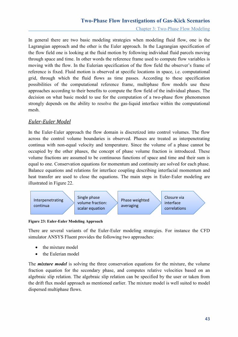
Two-Phase Flow Investigations of Gas-Kick Scenarios
Chapter 3: Two-Phase Flow Modeling
43
In general there are two basic modeling strategies when modeling fluid flow, one is the
Lagrangian approach and the other is the Euler approach. In the Lagrangian specification of
the flow field one is looking at the fluid motion by following individual fluid parcels moving
through space and time. In other words the reference frame used to compute flow variables is
moving with the flow. In the Eulerian specification of the flow field the observer’s frame of
reference is fixed. Fluid motion is observed at specific locations in space, i.e. computational
grid, through which the fluid flows as time passes. According to these specification
possibilities of the computational reference frame, multiphase flow models use these
approaches according to their benefits to compute the flow field of the individual phases. The
decision on what basic model to use for the computation of a two-phase flow phenomenon
strongly depends on the ability to resolve the gas-liquid interface within the computational
mesh.
Euler-Euler Model
In the Euler-Euler approach the flow domain is discretized into control volumes. The flow
across the control volume boundaries is observed. Phases are treated as interpenetrating
continua with non-equal velocity and temperature. Since the volume of a phase cannot be
occupied by the other phases, the concept of phase volume fraction is introduced. These
volume fractions are assumed to be continuous functions of space and time and their sum is
equal to one. Conservation equations for momentum and continuity are solved for each phase.
Balance equations and relations for interface coupling describing interfacial momentum and
heat transfer are used to close the equations. The main steps in Euler-Euler modeling are
illustrated in Figure 22.
Figure 23: Euler-Euler Modeling Approach
There are several variants of the Euler-Euler modeling strategies. For instance the CFD
simulator ANSYS Fluent provides the following two approaches:
the mixture model
the Eulerian model
The mixture model is solving the three conservation equations for the mixture, the volume
fraction equation for the secondary phase, and computes relative velocities based on an
algebraic slip relation. The algebraic slip relation can be specified by the user or taken from
the drift flux model approach as mentioned earlier. The mixture model is well suited to model
dispersed multiphase flows.
Interpenetrating continua
Single phase volume fraction: scalar equation
Phase weighted averaging
Closure via interface correlations

Two-Phase Flow Investigations of Gas-Kick Scenarios
Chapter 3: Two-Phase Flow Modeling
44
The Eulerian model is the most complex variant of the Euler-Euler models listed here. It
solves the momentum and continuity equations for each phase. Coupling is achieved through
the pressure and interphase exchange coefficients. Depending on the type of phases involved
the coupling is achieved by different models. The Eulerian model is used to model dispersed
multiphase flows like bubble columns, risers, particle suspension, and fluidized beds.
A general drawback of phase weighted averaging is the loss of information on the flow
details. Since the phase interface is not resolved, a certain phase volume fraction may
correspond to different flow morphologies. This is illustrated by the following two images,
showing two different types of flow but both showing an averaged volume fraction of 0.5. As
a consequence this approach should only be applied to model dispersed flow regimes.
Figure 24: Segregated Flow with = 0.5
Figure 25: Dispersed Flow with = 0.5
In general for an averaged two-fluid approach bubble sizes have to be smaller than the
discretized cell size. The approach is thus well suited to describe small-scale dispersed flow
like bubbly or droplet flow, where the scale of the interfacial structure is smaller than the
computational cell size.
Euler Lagrangian Approach
The Lagrangian discrete phase model (DPM) follows the Euler-Lagrange approach. The fluid
phase is treated as a continuum by solving the time-averaged Navier-Stokes equations, while
the dispersed phase is solved by tracking a large number of particles, bubbles, or droplets
through the calculated flow field. For the particles a Lagrangian approach is used, applying
the physical laws directly to each particle. Particle position, velocity are described as a
function of time. Particles can interact with the continuous (Euler) phase by exchanging
momentum, mass and energy. The main steps in Euler Lagrangian modeling approach are
illustrated in Figure 22. General simplifying assumption that are commonly made include
negligence of particle volume in the continuous phase solver
spherical particle shape
flow details in particle vicinity
representative particle used to model particle group
Depending on the assumptions made the validity of the modeling approach can be limited to a
certain volume fraction of the dispersed phase. Usually a dispersed phase volume fraction of
less than 10 – 12 % allows particle-particle interactions and the effect of the dispersed phase
on the continuous phase to be neglected.
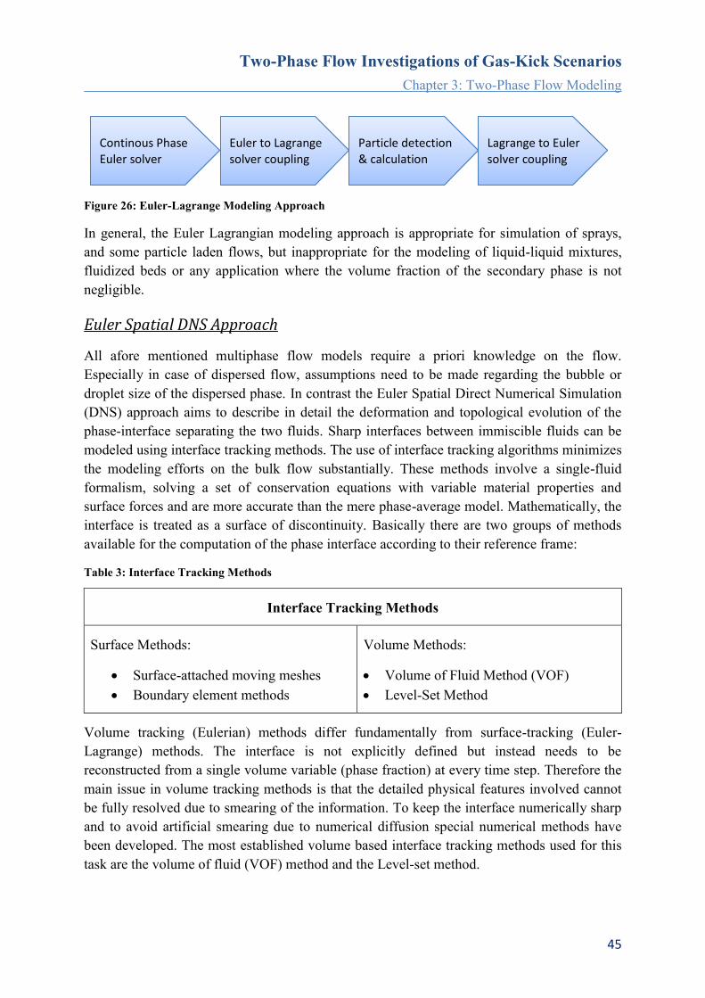
Two-Phase Flow Investigations of Gas-Kick Scenarios
Chapter 3: Two-Phase Flow Modeling
45
Figure 26: Euler-Lagrange Modeling Approach
In general, the Euler Lagrangian modeling approach is appropriate for simulation of sprays,
and some particle laden flows, but inappropriate for the modeling of liquid-liquid mixtures,
fluidized beds or any application where the volume fraction of the secondary phase is not
negligible.
Euler Spatial DNS Approach
All afore mentioned multiphase flow models require a priori knowledge on the flow.
Especially in case of dispersed flow, assumptions need to be made regarding the bubble or
droplet size of the dispersed phase. In contrast the Euler Spatial Direct Numerical Simulation
(DNS) approach aims to describe in detail the deformation and topological evolution of the
phase-interface separating the two fluids. Sharp interfaces between immiscible fluids can be
modeled using interface tracking methods. The use of interface tracking algorithms minimizes
the modeling efforts on the bulk flow substantially. These methods involve a single-fluid
formalism, solving a set of conservation equations with variable material properties and
surface forces and are more accurate than the mere phase-average model. Mathematically, the
interface is treated as a surface of discontinuity. Basically there are two groups of methods
available for the computation of the phase interface according to their reference frame:
Table 3: Interface Tracking Methods
Interface Tracking Methods
Surface Methods:
Surface-attached moving meshes
Boundary element methods
Volume Methods:
Volume of Fluid Method (VOF)
Level-Set Method
Volume tracking (Eulerian) methods differ fundamentally from surface-tracking (Euler-
Lagrange) methods. The interface is not explicitly defined but instead needs to be
reconstructed from a single volume variable (phase fraction) at every time step. Therefore the
main issue in volume tracking methods is that the detailed physical features involved cannot
be fully resolved due to smearing of the information. To keep the interface numerically sharp
and to avoid artificial smearing due to numerical diffusion special numerical methods have
been developed. The most established volume based interface tracking methods used for this
task are the volume of fluid (VOF) method and the Level-set method.
Continous Phase Euler solver
Euler to Lagrange solver coupling
Particle detection & calculation
Lagrange to Euler solver coupling

Two-Phase Flow Investigations of Gas-Kick Scenarios
Chapter 3: Two-Phase Flow Modeling
46
The volume of fluid method was initially presented by Hirt and Nichols (1981). Since then it
has been continuously developed and improved. The method is based on the idea to model the
movement of two immiscible fluids by one fluid with mixture properties. This reduces the
modeling effort to the solution of a single set of conservation equations and tracking the phase
volume fraction throughout the domain. The fields for all variables and properties are shared
by the phases and represent volume-averaged values, based on the local volume fractions.
Thus the variables and properties in any cell are either fully representative of a single phase or
a mixture of both phases. A scalar quantity f is used to define the volume fraction of each
phase in a cell. The phase indicator f represents the fraction of the volume of a mesh cell
occupied by a phase. Thus the volume fraction of the phases is defined as
𝛼𝑙 = 𝑓, 𝛼𝑔 = 1 − 𝑓
l volume fraction of liquid phase
g volume fraction of gas phase f phase indicator
The phase indicator f of a cell is either 1 if the cell is fully occupied with one phase or zero
when it is fully occupied with the other phase. Computational cells with a value of 0<f<1
indicate the instantaneous presence of both phases and are consequently cells that contain a
phase interface, as illustrated in Figure 27. The volume fractions of both phases sum to unity.
True Interface Volume Fractions
Figure 27: Volume Fractions on a Discrete Mesh (Pilliod and Puckett 2004)
The mixture properties needed for the transport equations are determined by the presence of
the phases in each computational cell. For two phase flow the definition is given by
𝜌𝑚 = 𝛼𝑙𝜌𝑙 + (1 − 𝛼𝑙)𝜌𝑔
𝜇𝑚 = 𝛼𝑙𝜇𝑙 + (1 − 𝜇𝑙)𝜌𝑔
𝜌𝑚 mixture density 𝜇𝑚 mixture viscosity 𝜇𝑙 viscosity of liquid phase 𝜌𝑔 density of gas phase
l volume fraction of liquid phase
Based on the mixture properties a single equation of motion is solved for the mixture fluid.
The resulting mixture velocity is valid for both phases.

Two-Phase Flow Investigations of Gas-Kick Scenarios
Chapter 3: Two-Phase Flow Modeling
47
𝜌𝑚 (𝜕˅
𝜕𝑡+ ˅ ∙ ∇˅) = −∇𝑝 + ∇ ∙ (𝜇𝑚(∇˅ + (∇˅)𝑇)) + 𝜌𝑔
This equation is dependent on the volume fractions through the material properties only. The
volume fractions are propagated through the domain by solving a scalar convection equation
defined by
𝜕𝑓
𝜕𝑡+ ∇ ∙ 𝑓𝑈𝑚 = 0
Um mixture velocity f phase indicator
The transport equation for the volume fraction is satisfying mass conservation of both phases.
Within the volume of fluid method a continuity equation based on the volume fraction is
defined for each phase. The tracking of the phase interface in case of two phase flow is
accomplished by the solution of the volume fraction equation of one phase. The volume
fraction of the other phase is computed based on the constraint that the volume fractions of
both phases sum to unity.
𝜕
𝜕𝑡(𝛼𝑙𝜌𝑙) + ∇ ∙ (𝛼𝑙𝜌𝑙˅) = 𝑆𝛼𝑙
+ (𝑔𝑙 − 𝑙𝑔)
𝛼𝑔 + 𝛼𝑙 = 1
𝑆𝛼𝑙 source term
𝑔𝑙 mass transfer rate, gas to liquid
𝑔𝑙 mass transfer rate, liquid to gas
Using the explicit time discretization leads to
𝛼𝑙𝑛+1𝜌𝑙
𝑛+1 − 𝛼𝑙𝑛𝜌𝑙
𝑛
Δ𝑡𝑉 + ∑(𝜌𝑙𝑈𝑓
𝑛𝛼𝑙,𝑓𝑛 )
𝑓
= [𝑆𝛼𝑙+ (𝑔𝑙 − 𝑙𝑔)]𝑉
𝑛 + 1 index of current time step 𝑛 index of previous time step
𝑈𝑓 volume flux through cell face
𝛼𝑙,𝑓 volume faction value at cell face (computed by interface reconstruction scheme)
𝑉 volume of cell
Storing phase volume fractions per cell rather than explicit interface geometry eases the
simulation of multiphase flows. However in order to compute the phase fluxes at the cell
faces information is need about the interface geometry and orientation. Since the volume
fraction has large gradients at the interface the application of a standard difference scheme for
spatial discretization would result in numerical smearing and interfaces would lose their
definition. Waclawczyk and Koronowicz (2005) showed that most convective differencing
schemes applied to the volume fraction convection equation introduce too much numerical
diffusion and smear the step profile of the interface over several cells. To avoid this smearing,

Two-Phase Flow Investigations of Gas-Kick Scenarios
Chapter 3: Two-Phase Flow Modeling
48
the use of higher order or blending differencing schemes like CICSAM (Ubbink 1997) or
geometrical reconstruction of the phase interface (Youngs 1982) are suggested. The CICSAM
scheme is particularly suitable for fluid pairs with a high viscosity ratio. This is the crucial
task to provide accurate advection of the fluid phases (Pilliod and Puckett 2004). The phase
fluxes are obtained by these interface reconstruction schemes. Within the CICSAM scheme
the computation of convection and diffusion fluxes through the cell faces is based on the
following donor-acceptor scheme
𝜙𝑓 = 𝜙𝑑 + 𝛽∇𝜙𝑑
𝜙𝑓 volume fraction value at cell face
𝜙𝑑 donor cell volume fraction value
𝛽 slope limiter value
∇𝜙𝑑 donor cell volume fraction gradient
The scheme identifies one cell as a donor of an amount of fluid from one phase and
neighboring cell as the acceptor of that same amount of fluid. More details on the theory of
the compressive interface capturing scheme (CICSAM) can be found in the work of Ubbink
(1997).
Finally the energy equation within the volume of fluid method is defined as
𝜕
𝜕𝑡(𝜌𝑚𝐸) + ∇ ∙ (˅(𝜌𝑚𝐸 + 𝑝)) = ∇ ∙ (𝑘𝑒𝑓𝑓∇𝑇) + 𝑆ℎ
𝑘𝑒𝑓𝑓 effective thermal conductivity, shared by the phases
𝑆ℎ source term
Energy E and temperature T are defined as mass averaged variables according to
𝐸 =𝛼𝑙𝜌𝑙𝐸𝑙 + 𝛼𝑔𝜌𝑔𝐸𝑔
𝛼𝑙𝜌𝑙 + 𝛼𝑔𝜌𝑔
𝑇 =𝛼𝑙𝜌𝑙𝑇𝑙 + 𝛼𝑔𝜌𝑔𝑇𝑔
𝛼𝑙𝜌𝑙 + 𝛼𝑔𝜌𝑔
Compared with the Euler-Euler and the Euler-Lagrange approach described earlier, the volume of
fluid method and other interface capturing approaches can be thought of as an Euler Spatial Direct
Numerical Simulation (DNS) of interface motion (not of turbulence), where no closure
assumptions for the interfacial area evolution are needed. A prerequisite for the application of
interface capturing methods is that interfacial length scales have to be several times larger
than the grid size. Meaning the computational grid needs to be refined to such an extent that
most computational cells are occupied by a single fluid and phase interfaces are represented
by as few cells as possible. The volume of fluid method has its strength in modeling large-
scale interfacial structures, with a grid fine enough to capture the phase interface allowing a
detailed resolution of surface phenomena. Interface tracking methods are best suited for these
flows as they represent the interface topology rather accurately and are built within a single
fluid formalism. Applications of the VOF model include stratified and free-surface flows, as
well as steady or transient tracking of any liquid-gas interface.

Two-Phase Flow Investigations of Gas-Kick Scenarios
Chapter 3: Two-Phase Flow Modeling
49
Multi-Phase Flow Simulators
In this section existing multi-phase flow simulators are listed that are most relevant for the
simulation of multi-phase flow in pipelines and wellbores. It is not the intention to give a
complete summary of existing simulation tools but to list the most common commercial
products and models behind.
Transient simulations of gas-liquid flow in pipelines and wellbores involve elaborate
computer codes and require considerable computational efforts. Consequently it has always
been desired to simplify the modeling effort but still achieve realistic answers. Several codes
have been proposed for this task so far, and supported by the oil and gas industry.
Historically, OLGA is the first of these codes. It is today probably the most well documented
and advanced multi-phase transient pipe flow simulator with a global market share of about
90%. OLGA, the name is short for “oil and gas simulator”, was originally developed in the
80s by Statoil (Bendiksen et al. 1987, 1991) and then continued further by SINTEF. The code
is capable of modeling a wide range of scenarios by varying fluid properties, pressure,
temperature, geometry, trajectory, influx rate, circulation rate, friction, etc. The software is
based on a one-dimensional, two-fluid model. For the gas and liquid phases, the model
consists of separate conservation equations for both mass and momentum. A single energy
conservation equation is used for the liquid and gas phase. Solving the system of conservation
equations requires averaging and simplification. OLGA also involves flow-pattern predictions
and requires closure relationships to replace the information lost in the simplification process.
Also to mention is the PLAC code developed in England (Black et al. 1990), it is also a two-
fluid model. Then there is the TACITE code developed at the Institut français du pétrole, it is
based on drift flux type models (Pauchon et al. 1993, 1994). Another simulator based on a
drift flux model is TRAFLOW, developed by the Shell Oil Company. Then there is LedaFlow
another multiphase flow simulator developed by Sintef in Norway in partnership with Total
and ConocoPhillips and finally commercialized by Kongsberg. LedaFlow is a highly
sophisticated flow simulator solving mass, energy, and momentum conservation for each
phase.
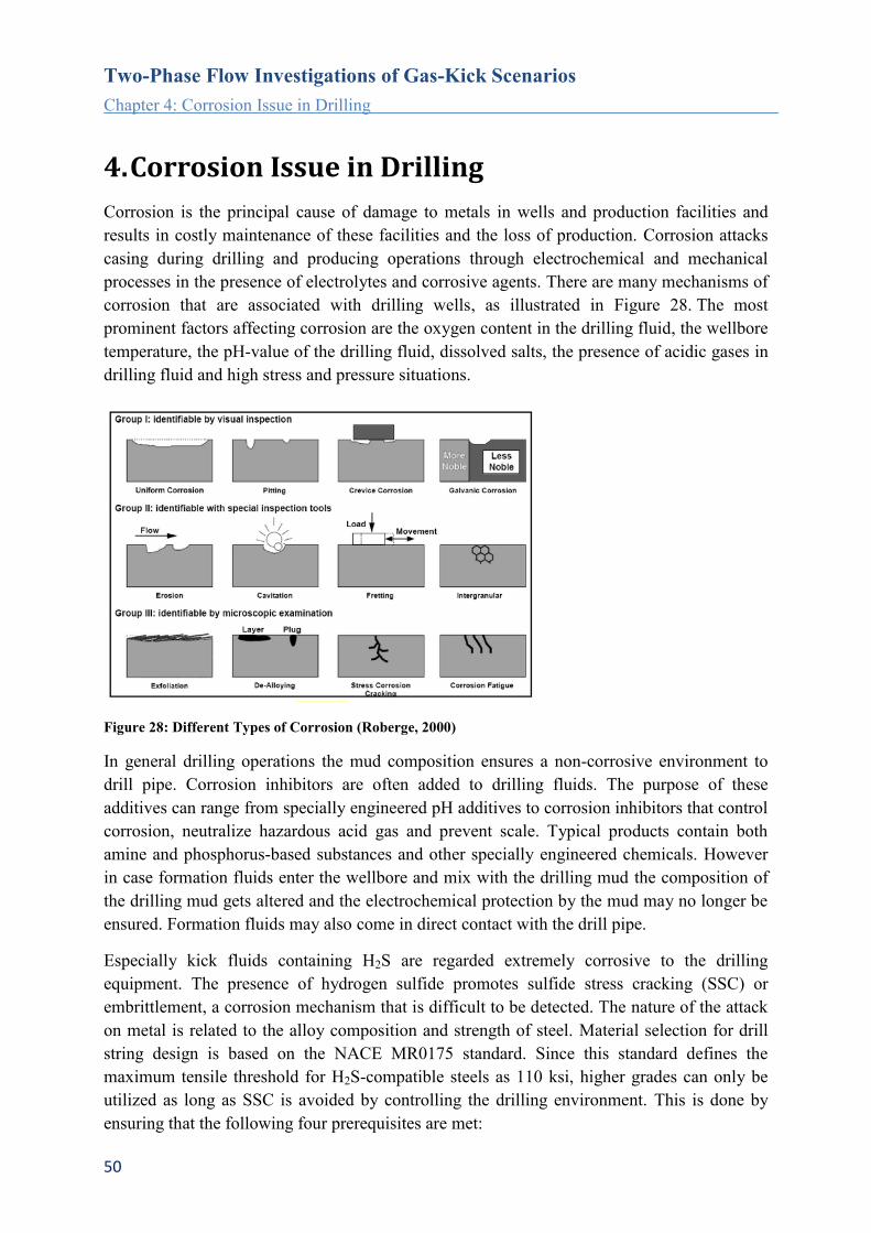
Two-Phase Flow Investigations of Gas-Kick Scenarios
Chapter 4: Corrosion Issue in Drilling
50
4. Corrosion Issue in Drilling
Corrosion is the principal cause of damage to metals in wells and production facilities and
results in costly maintenance of these facilities and the loss of production. Corrosion attacks
casing during drilling and producing operations through electrochemical and mechanical
processes in the presence of electrolytes and corrosive agents. There are many mechanisms of
corrosion that are associated with drilling wells, as illustrated in Figure 28. The most
prominent factors affecting corrosion are the oxygen content in the drilling fluid, the wellbore
temperature, the pH-value of the drilling fluid, dissolved salts, the presence of acidic gases in
drilling fluid and high stress and pressure situations.
Figure 28: Different Types of Corrosion (Roberge, 2000)
In general drilling operations the mud composition ensures a non-corrosive environment to
drill pipe. Corrosion inhibitors are often added to drilling fluids. The purpose of these
additives can range from specially engineered pH additives to corrosion inhibitors that control
corrosion, neutralize hazardous acid gas and prevent scale. Typical products contain both
amine and phosphorus-based substances and other specially engineered chemicals. However
in case formation fluids enter the wellbore and mix with the drilling mud the composition of
the drilling mud gets altered and the electrochemical protection by the mud may no longer be
ensured. Formation fluids may also come in direct contact with the drill pipe.
Especially kick fluids containing H2S are regarded extremely corrosive to the drilling
equipment. The presence of hydrogen sulfide promotes sulfide stress cracking (SSC) or
embrittlement, a corrosion mechanism that is difficult to be detected. The nature of the attack
on metal is related to the alloy composition and strength of steel. Material selection for drill
string design is based on the NACE MR0175 standard. Since this standard defines the
maximum tensile threshold for H2S-compatible steels as 110 ksi, higher grades can only be
utilized as long as SSC is avoided by controlling the drilling environment. This is done by
ensuring that the following four prerequisites are met:

Two-Phase Flow Investigations of Gas-Kick Scenarios
Chapter 4: Corrosion Issue in Drilling
51
Maintain the drilling fluid density to minimize formation fluid influx
Neutralize inflowing H2S by maintaining a mud pH of 10 or higher
Utilize sulfide chemical scavengers and/or corrosion inhibitors
Use oil-base drilling fluids
These requirements are fulfilled during controlled drilling operations. During a kick situation
three of the aforementioned preconditions can be lost rapidly (sufficient fluid
density/hydrostatic head, high mud pH and sufficient presence of scavengers) and drill string
is exposed to a highly corrosive environment. Even without prolonged exposure of the drill
string to such environments, due to the practical inability to actually measure SSC it is
difficult to assess whether the drill pipe needs to be replaced or can stay in place. Therefore, if
it is possible to accurately predict downhole pH developments due to influx and mixing of
H2S-containing reservoir fluids with the high-pH drilling mud, this will provide a decision
criteria to whether circulate the kick out, kill the well and continue drilling or to kill the well
and immediately pull the string out of the hole to replace it. Such simulations ultimately help
to develop a sound risk assessment based on pH, H2S concentration, pressures and exposure
times.
Corrosion Modeling
Corrosion prediction in multiphase flow is a challenging task. Most existing corrosion models
are only applicable to single phase flow. To extend the corrosion model capability to
multiphase flow, the mass transfer and the turbulent diffusivity correlations in the models
have to be modified to properly calculate the mass flux of corrosion species (Wang et.al.
2003).Very little work has been done so far identifying the phase interface area development
through CFD modeling – mostly due to the massive computational effort required to model
these environments. To assess the role of H2S in the corrosion process a detailed
understanding of the underlying multiphase flow mechanisms is needed. Flow features and
spatial distribution of phases are often described by a set of well-known flow patterns. Each
flow pattern shows certain characteristics with respect to corrosion rate. This is certainly true
as each flow pattern determines the mass transfer rate and phase interface area available for
H2S dissolution.
For pipeline and wellbore applications, corrosion models need to be able to predict corrosion
rates, in both single and multiphase flow conditions. It is well known that the flow variations
along pipelines, such as flow regime, water wetting and liquid flow velocity, have significant
effects on the corrosion process in multiphase flow conditions (Jepson et al. 1997). Flow
patterns like slugging are very turbulent and can remove corrosion protection as well as
corrosion products. Corrosion can be self-limiting, due to formation of corrosion scales that
protect the metal underneath. The problem with slug flow is that it removes these scales and
the pipe is always exposed to the corrosive environment the repeated impact of the slugs.
Therefore corrosion models need to be adapted and coupled with multiphase flow simulators
to compute the effects of multiphase flow.
Two-Phase Flow Investigations of Gas-Kick Scenarios
Chapter 4: Corrosion Issue in Drilling
52
There have been efforts to provide this coupling in the area of acid gas corrosion. Past
research efforts resulted in the implementation of CO2 corrosion models into the three–phase
fluid flow simulator OLGA. Three empirical and semi-empirical corrosion models, NORSOK
M-506, de Waard 1995, and IFE top-of-line corrosion, have been embedded as modules in
OLGA. Wand and Nesic 2003 describe the coupling of a more mechanistic corrosion model
with a comprehensive multiphase fluid flow model. But sour gas corrosion involving H2S is
currently not considered.
Sulfide Stress Cracking
High-strength steel pipes used in drilling and completion of oil and gas wells may exhibit
delayed failure in environments containing hydrogen sulfide. This type of failure is referred to
as sulfide stress cracking (SSC) and occurs when metal is in tension and exposed to H2S and
water. The basic cause of sulfide stress cracking is embrittlement resulting from hydrogen
absorbed into steel during corrosion in sour environments.
Sour gas is natural gas or any other gas that is corrosive due to a significant content of
hydrogen sulfide (H2S). Sour environments are defined when the partial pressure of hydrogen
sulfide is above 0.0003 MPa. Partial pressure is determined by multiplying the mole fraction
of H2S in the gas with the system pressure. At higher partial pressures, the corrosion rate on
carbon steel is substantially increased by means of making the water phase more acidic and by
forming iron sulfide scale.
The presence of water due to its electrolytic nature is needed for corrosion to take place.
Although hydrogen sulfide gas can cause embrittlement, water must be present for sulfide
stress cracking to occur. Hydrogen sulfide is moderately soluble in water compared to oil
based fluids. Hydrogen sulfide can be destroyed by oxidation when dissolved in water.
Dissolved H2S is forming a weak acid and can be regarded as a cathodic species. In contrast
to water based drilling mud systems, oil-based drilling muds prevent the completion of the
galvanic cell and are therefore very effective in reducing corrosion to the drilling equipment
(Chilingar et al. 2008). Certain chemicals, when added to the oil-base muds, make the steel
surface oil wet and protect it against corrosion.
Sulfide stress cracking is common in high strength steels containing Martensite. It can also
occur in ferritic steels. The NACE standard defines SSC as the cracking of a metal under the
combined action of tensile stress and corrosion in the presence of water and hydrogen
sulfide. SSC is generally limited to steels having a hardness of 22 or greater on the Rockwell
C scale. The occurrence of sulfide stress cracking depends on the interaction of the following
parameters:
pipe material, i.e. chemical composition, strength, heat treatment, and microstructure
of the material
pH value of the solution, i.e. concentration of hydrogen ions
total tensile stress
temperature
Two-Phase Flow Investigations of Gas-Kick Scenarios
Chapter 4: Corrosion Issue in Drilling
53
exposure time
SSC is a type of hydrogen induced cracking (HIC) in which the primary poison is the
evolution of atomic hydrogen. The source of atomic hydrogen is described by the following
reaction scheme:
𝐹𝑒 + 𝐻2𝑆 + 𝐻2𝑂 ⇔ 𝐹𝑒𝑆𝑥 + 𝐻2 + 𝐻2𝑂
Hydrogen sulfide reacts with iron at the pipe surface, forming iron sulfide (FeS) scale and
liberating two hydrogen atoms. The hydrogen ions diffuse into the steel and initially
accumulate at anomalies in the metal lattice. Continuous supply and diffusion of hydrogen
ions results in combination of atomic hydrogen to hydrogen molecules H2 inside the metal
lattice. The size of the molecules exceeds the available interstitial space and causes
embrittlement between the grains of the metal. Due to the reduced metal ductility cracks will
initiate, leading to crack propagation in a direction perpendicular to the tensile stress. This
affects a normally ductile material making it hard and brittle. Delayed cracking is often
associated with high strength of steel. High concentrations of hydrogen sulfide may act to
inhibit corrosion of mild steel (Watkins and Wright 1953). However, in the case of high-
strength steels, high concentrations of hydrogen sulfide produce rapid embrittlement.
Influence of Flow Field on Corrosion
The presence of H2S leads to the formation of various forms of iron sulfide scales, some of
them can be very protective. The formation of surface scales is therefore an important
parameter affecting the corrosion rate. Surface scales are predominantly a result of direct
chemical reaction between H2S and the steel surface, but can also result from precipitation in
supersaturated solutions over long periods of time (Sun and Nesic 2007).
Sun and Nesic (2007) conducted experiments in galvanic cells to investigate the mechanisms
and kinetics of mild steel corrosion in H2S environments. The dominant iron sulfide scale that
formed under their test conditions was Mackinawite. Mackinawite scale has been shown to
form extremely fast (less than seconds). “This film is very thin (<<1µm) but dense and acts
as a solid state diffusion barrier for the sulfide species involved in the corrosion reaction. The
thin Mackinawite film continuously goes through a cyclic process of growth, cracking and
delamination, what generates the outer sulfide layer which thickens over time (typically
>1µm) and also presents a diffusion barrier; this outer sulfide layer is very porous and rather
loosely attached, over time it may crack, peel and spall, a process aggravated by the flow.”
The Mackinawite scale may dissolve into the solution depending on the solution saturation
level. Srinivasan and Kane (1996) observed an increase in dissolution with decreasing pH,
until a range of pH=2 to pH=3 where no more Mackinawite can be detected on the steel
surface.
Figure 29 illustrates the molecular diffusion of both hydrogen sulfide and atomic hydrogen
through the scale on the steel surface. The hydrogen sulfide arriving at the steel surface will
directly react with the steel and form iron sulfide at the inner interface whereas the hydrogen
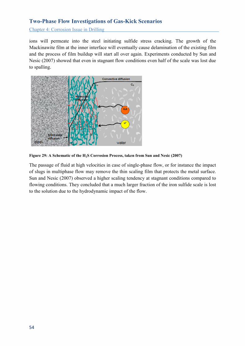
Two-Phase Flow Investigations of Gas-Kick Scenarios
Chapter 4: Corrosion Issue in Drilling
54
ions will permeate into the steel initiating sulfide stress cracking. The growth of the
Mackinawite film at the inner interface will eventually cause delamination of the existing film
and the process of film buildup will start all over again. Experiments conducted by Sun and
Nesic (2007) showed that even in stagnant flow conditions even half of the scale was lost due
to spalling.
Figure 29: A Schematic of the H2S Corrosion Process, taken from Sun and Nesic (2007)
The passage of fluid at high velocities in case of single-phase flow, or for instance the impact
of slugs in multiphase flow may remove the thin scaling film that protects the metal surface.
Sun and Nesic (2007) observed a higher scaling tendency at stagnant conditions compared to
flowing conditions. They concluded that a much larger fraction of the iron sulfide scale is lost
to the solution due to the hydrodynamic impact of the flow.

Two-Phase Flow Investigations of Gas-Kick Scenarios
Chapter 4: Corrosion Issue in Drilling
55
Corrosion Modeling Approach
It is known that sulfide stress cracking is influenced by three general classes of variables:
environment, metallurgy, and state of stress. This work focuses on the effect of environmental
factors like flow morphology, concentration of H2S, and temperature (the susceptibility to
sulfide stress cracking increases with increasing H2S concentration and decreases with
increasing pH). Although hydrogen sulfide gas, like gaseous hydrogen, can cause
embrittlement, water ordinarily must be present for sulfide stress cracking to occur. This puts
water based muds into the focus when trying to predict the corrosive attack of a gas-kick
event. To calculate the amount of dissolved H2S in the flow, models for gas solubility and
mass transfer need to be specified.
Gas Solubility
The gas solubility defines the maximum amount of gas that can be dissolved in a fluid at a
specific temperature and pressure. Whereas bubble pressure determines at which pressure this
gas would evolve from solution. The formation volume factor of the saturated fluid describes
the volume variation of the saturated fluid due to the dissolved gas. These properties play an
important role when dealing with the invasion of formation gas into oil-based drilling muds.
According to literature larger amounts of gas can be dissolved in oil based muds compared to
water-based muds. This fact is important when considering the volumetric expansion of rising
gas bubbles with decreasing depth. The high solubility of natural gas in oil-based drilling
fluids poses a difficulty in detecting gas-kicks. Surface responses are initially dampened and
reduced well below those normally seen with water based muds. When a gas-drilling fluid
mixture is circulated toward the surface, gas will evolve from solution and expand rapidly,
due to the reduced pressure. This swelling behavior is not so pronounced in water based muds
as a consequence of the lower gas solubility.
The problems associated with natural gas solubility in drilling fluids have been studied since
1981. The main focus of these studies was put on oil based drilling fluids and the danger
associated with the volumetric expansion when the gas evolves from the solution. O’Brien
(1981) suggested that the gas solubility in an oil based drilling fluid could be 10 to 100 times
greater than in a water based mud. Therefore the high solubility of H2S in oil based muds is of
crucial importance when it comes to kick detection. As a consequence literature presents a
large number of studies dealing with the dissolution of natural gas in oil based or synthetic
drilling fluids, but these types of mud are not subject of this work
For water based mud, gas solubility is generally neglected when predicting gas-kick behavior.
The volumetric influence of the gas on the water based mud is insignificant. Instead the
chemical processes are of great importance. The corrosive potential in water based drilling
fluids is much larger compared to oil based drilling fluids. The presence of hydrogen sulfide
(H2S) and free water can cause severe corrosion problems. The first step in this process is the
dissolution of the gas.

Two-Phase Flow Investigations of Gas-Kick Scenarios
Chapter 4: Corrosion Issue in Drilling
56
To characterize the dissolution of gas in a liquid the following mechanistic view of
dissolution as a stepwise process is very helpful. Initially gas and liquid molecules are in
separate phases. When dissolution begins a gas molecule has to be separated from its adjacent
molecules and transferred to the phase interface. This transport is done by convection and/or
diffusion. At the interface the molecule dissolves into the other phase and is then transported
again by convection and/or diffusion to fill a vacancy in the liquid. This simplistic view helps
us to think about dissolution as a transport process and allows its modeling as mere mass
transfer and inherently interfacial phenomenon.
The process of dissolution will continue until a maximum concentration of gas molecules in
the liquid phase is reached, termed the gas solubility. In general the maximum amount of gas
that can go into solution is proportional to pressure, temperature, and chemical constituents of the
liquid. For instance polar solutes tend to dissolve best in polar solvents while non-polar solutes
tend to dissolve best in non-polar solvents. H2S is considerably more soluble in organic
compounds than in aqueous solutions, except at high pH, the solubility increasing with
increase in aromatic nature and decreasing with increase in paraffin and polar nature.
In the wellbore gas solubility is mainly affected by temperature and pressure condition. At
high pressure conditions the behavior of gas deviates from non-ideal gas behavior. This can
be expressed by the compressibility factor Z:
𝑍 =𝑃𝑉
𝑛𝑅𝑇
where
P pressure V gas volume n number of moles of gas R universal gas constant T temperature
The solubility of gas in water is commonly calculated by Henry’s law. This approach is
appropriate as long as the pressure is low and the gas is behaving ideal. In case of high
pressure conditions the solubility computations need to be improved by using a modified form
of Henry’s law. The modification of Henry’s law is usually based on experimental data, and is
specific for a certain gas and solvent.
There have been many experimental studies on the solubility of H2S in aqueous solutions.
However, as H2S solutions are very corrosive, experimental measurements a generally limited
to a relatively small range of temperatures, pressures, ionic strength, and the data is in general
very scattered and difficult to use (Duan et al. 2007). Duan et al. summarized existing
solubility models for H2S in aqueous solutions as well as existing experimental data. Based on
the chemical potential of H2S in the liquid and in the gas phase, they presented a novel model
covering a large temperature and pressure range with high accuracy. Calculated gas
solubilities based on this model are illustrated in Figure 30. A big advantage of the model is

Two-Phase Flow Investigations of Gas-Kick Scenarios
Chapter 4: Corrosion Issue in Drilling
57
that it can also be applied to more complex systems, i.e. aqueous solutions with multiple
components.
Figure 30: Solubility of H2S in Pure Water Calculated by the Model of Duan et al. (2007)
The solubility of H2S first increases linearly with increasing pressure, but at high pressures the
slope gradually decreases.
Mass Transfer Formulation
Gas dissolution can be described as the transfer of gas particles from the gas phase into the
liquid solvent. This process can be regarded as a stepwise process. At the beginning of this
process the gas and the liquid particles are spatially separated in the gas and liquid phases.
The dissolution process starts with the separation of a single gas particle (solute) from the gas
phase without leaving a hole. Next the gas particle is transported to the phase interface, where
it gets transferred from the gas phase to the liquid phase (solvent), and eventually transported
and inserted into a vacancy in the liquid phase. The dissolution process is accompanied by a
change in the Gibbs free energy of the system, meaning the overall Gibbs free energy of the
solution is decreased compared to the Gibbs free energy of the separated gas and liquid
phases. The Gibbs energy is a thermodynamic potential that is minimized when a system
reaches chemical equilibrium.
Dissolution is a kinetic process, and is generally quantified by a mass transfer rate. This rate is
defined as the amount of solute that goes in solution per unit time under certain conditions
regarding temperature, pressure, phase interface, solvent composition, flow regime etc. Mass
transfer rate prediction is of great importance in computing corrosion rates.
The simplest approach to calculate mass transfer rate is by using Henry’s law. This gas law,
formulated by William Henry in 1803 states "At a constant temperature, the amount of a
given gas that dissolves in a given type and volume of liquid is directly proportional to the
Two-Phase Flow Investigations of Gas-Kick Scenarios
Chapter 4: Corrosion Issue in Drilling
58
partial pressure of that gas in equilibrium with that liquid." The proportionality factor
relating partial pressure and gas solubility factor is called the Henry's law constant.
𝑘 =𝐶𝑆
𝑝𝑔𝑎𝑠
CS gas solubility k Henry’s law constant pgas partial pressure of the gas under equilibrium
Henry’s law describes the solubility of a specific gas in a particular stagnant solvent at a fixed
temperature. Therefore Henry’s law constants can be found in literature for a variety of solute
and solvent pairs. Henry’s law has a couple of limitations, i.e. it works only for molecules at
equilibrium, it cannot be applied when there is a chemical reaction between the solute and the
solvent, and moreover it does not work for gasses at high pressures. For instance Zheng et al.
(2002) mention that gas dissolution computed by Henry’s law deviates significantly from
actual values in high-pressure conditions. Using Henry’s law to calculate mass transfer is
equivalent to determine the maximum amount of gas that will be dissolved at steady state
conditions. Such an approach is not taking into account the movement of fluids, gas
concentration variations in the solvent and available interface area between the phases.
When interested in the transient simulation of the gas dissolving process in a liquid it is
necessary to formulate a model for mass transfer rate calculation. To do so the dissolution
operation is understood as an interfacial phenomenon driven by a concentration difference.
The temporal course of dissolution is also strongly affected by interfacial and bulk phase
hydrodynamics responsible for the convective transport of species apart from molecular
diffusion. The dissolution process is usually characterized by a mass transfer coefficient, K,
relating the mass transfer rate with concentration gradient and available interface area as
follows:
𝑑𝑚
𝑑𝑡= 𝐾𝑀𝐴(𝐶𝑆 − 𝐶0)
where
m mass [kg] K mass transfer coefficient [m/s] M molecular weight of gas [kg/mole] A interface area [m²] CS gas solubility [mole/m³] C0 concentration of dissolved gas [mole/m³]
The equation above is summarizing the stepwise process of dissolution and characterizes it
with the parameters interface area, concentration difference and mass transfer coefficient. The
concentration difference is defined as the difference between maximum possible solute
concentration and current concentration. Calculation of concentration difference is straight
forward, based on the solubility model and updated concentration values. The available
interface area for dissolution is more difficult to determine. In case of perfectly round gas

Two-Phase Flow Investigations of Gas-Kick Scenarios
Chapter 4: Corrosion Issue in Drilling
59
bubbles the interface area is clearly defined and can be easily be calculated. The situation
becomes more difficult with local deformations of the interface or irregular shapes that are not
being resolved in the computation of the phase interface. In such a case a first order estimate
for the interface area is used and additional local shape effects need to be included by
alteration of the mass transfer coefficient. The mass transfer coefficient is the most complex
parameter. When looking at the above equation it is clear that the mass transfer coefficient
needs to incorporate effects of flow regime, diffusion, fluid composition etc. To account for
variations in mass transfer rate due to chemical reactions an enhancement factor E can be
introduced in the above equation, leading to:
𝑑𝑚
𝑑𝑡= 𝐸𝐾𝑀𝐴(𝐶𝑆 − 𝐶0)
Mass transfer coefficients can be estimated based on theoretical equations, empirical
correlations, and analogies that are functions of fluid properties, system properties, and
hydrodynamics of the flow. Mass transfer coefficients depend on the shape and size of the
phase interface, gas diffusivity in liquids, the average fluid velocity and turbulent intensity.
Several theoretical mass transfer models are available to define the mass transfer coefficient.
Among these are the film theory, the boundary layer theory, the penetration and the surface
renewal theory. It is not scope of this work to explain these theories, but instead to point out
an appropriate definition for a mass transfer coefficient applicable to the current modeling
subject.
Mass transfer coefficients are rarely reported as individual values. More commonly the mass
transfer coefficient is described using a Sherwood correlation for a certain flow configuration,
i.e. a situation with a known contribution of convection and diffusion. The Sherwood number
(also called the mass transfer Nusselt number in analogy to heat transfer) is basically a
dimensionless number used to characterize mass transfer operations. It is defined as the ratio
of convective to diffusive mass transport.
𝑆ℎ = 𝐾𝐿
𝐷=
𝑐𝑜𝑛𝑣𝑒𝑐𝑡𝑖𝑣𝑒 𝑚𝑎𝑠𝑠 𝑡𝑟𝑎𝑛𝑠𝑓𝑒𝑟
𝑑𝑖𝑓𝑓𝑢𝑠𝑖𝑣𝑒 𝑚𝑎𝑠𝑠 𝑡𝑟𝑎𝑛𝑓𝑒𝑟
where
K mass transfer coefficient L characteristic length D mass diffusivity
In other terms the Sherwood number is a function of the Reynolds number (Re) and the
Schmidt number (Sh), with the Schmidt number representing the diffusion portion and the
Reynolds number the convective contribution to the mass transfer process.
𝑆ℎ = 𝑓(𝑅𝑒, 𝑆𝑐)
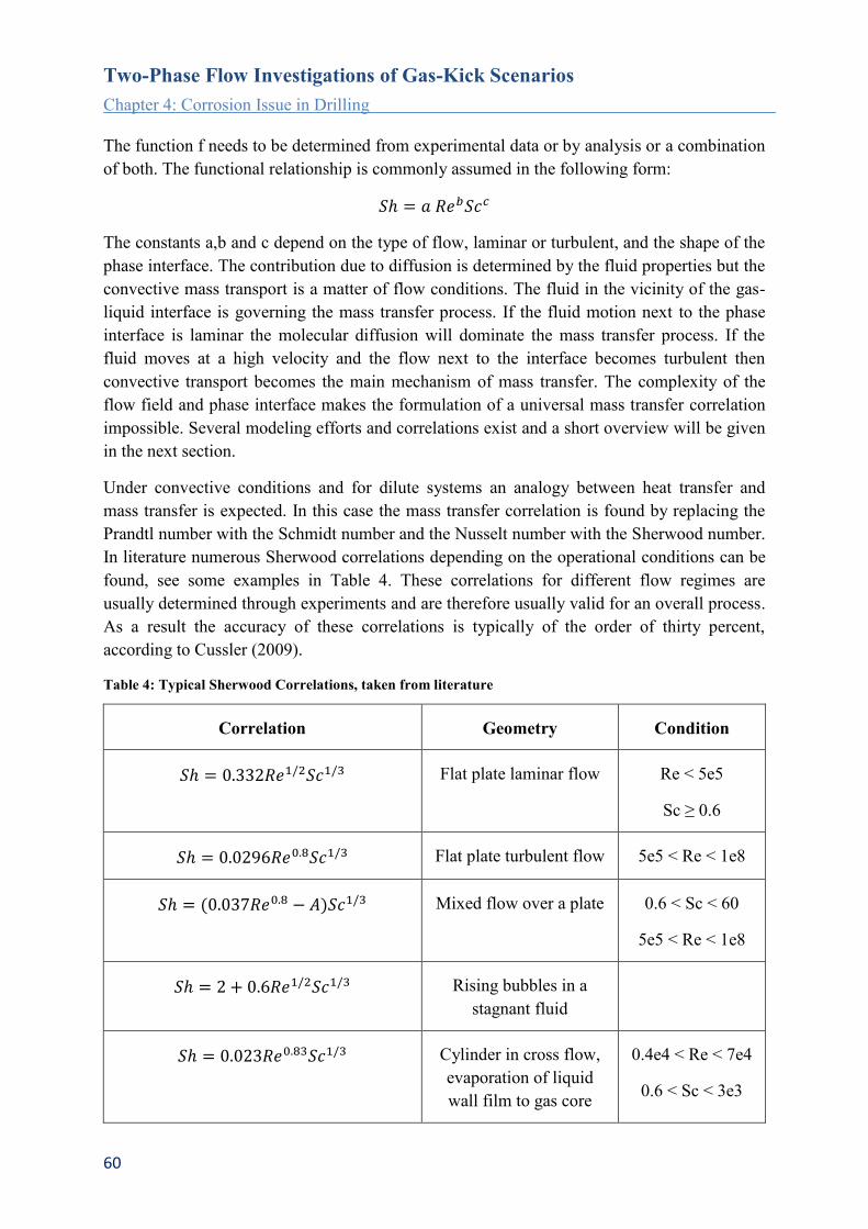
Two-Phase Flow Investigations of Gas-Kick Scenarios
Chapter 4: Corrosion Issue in Drilling
60
The function f needs to be determined from experimental data or by analysis or a combination
of both. The functional relationship is commonly assumed in the following form:
𝑆ℎ = 𝑎 𝑅𝑒𝑏𝑆𝑐𝑐
The constants a,b and c depend on the type of flow, laminar or turbulent, and the shape of the
phase interface. The contribution due to diffusion is determined by the fluid properties but the
convective mass transport is a matter of flow conditions. The fluid in the vicinity of the gas-
liquid interface is governing the mass transfer process. If the fluid motion next to the phase
interface is laminar the molecular diffusion will dominate the mass transfer process. If the
fluid moves at a high velocity and the flow next to the interface becomes turbulent then
convective transport becomes the main mechanism of mass transfer. The complexity of the
flow field and phase interface makes the formulation of a universal mass transfer correlation
impossible. Several modeling efforts and correlations exist and a short overview will be given
in the next section.
Under convective conditions and for dilute systems an analogy between heat transfer and
mass transfer is expected. In this case the mass transfer correlation is found by replacing the
Prandtl number with the Schmidt number and the Nusselt number with the Sherwood number.
In literature numerous Sherwood correlations depending on the operational conditions can be
found, see some examples in Table 4. These correlations for different flow regimes are
usually determined through experiments and are therefore usually valid for an overall process.
As a result the accuracy of these correlations is typically of the order of thirty percent,
according to Cussler (2009).
Table 4: Typical Sherwood Correlations, taken from literature
Correlation Geometry Condition
𝑆ℎ = 0.332𝑅𝑒1/2𝑆𝑐1/3 Flat plate laminar flow Re < 5e5
Sc ≥ 0.6
𝑆ℎ = 0.0296𝑅𝑒0.8𝑆𝑐1/3 Flat plate turbulent flow 5e5 < Re < 1e8
𝑆ℎ = (0.037𝑅𝑒0.8 − 𝐴)𝑆𝑐1/3 Mixed flow over a plate 0.6 < Sc < 60
5e5 < Re < 1e8
𝑆ℎ = 2 + 0.6𝑅𝑒1/2𝑆𝑐1/3 Rising bubbles in a
stagnant fluid
𝑆ℎ = 0.023𝑅𝑒0.83𝑆𝑐1/3
Cylinder in cross flow,
evaporation of liquid
wall film to gas core
0.4e4 < Re < 7e4
0.6 < Sc < 3e3

Two-Phase Flow Investigations of Gas-Kick Scenarios
Chapter 4: Corrosion Issue in Drilling
61
(Chilton-Colburn)
𝑆ℎ = 0.3 + [0.62𝑅𝑒1
2𝑆𝑐1
3 [1 +
(0.4
𝑆𝑐)
2
3]
−1
4
] [1 + (𝑅𝑒
282000)
5
8]
4
5
Cylinder in cross flow
(Churchill-Bernstein
equation)
ScRe ≥0.2
Mass transfer is assumed to be strongly affected by turbulent eddies around the phase
interface. Introducing the concept of turbulence instead of using empirical parameters in the
definition of the mass transfer coefficient is subject of the penetration theory and the surface
renewal theory.
The penetration theory was proposed by Higbie in 1935. He regarded the gas-liquid interface
to be made up of a variety of small liquid elements, which are continuously brought up to the
surface from the bulk of the liquid by the motion of the liquid phase itself. Mass transfer takes
place by diffusion in the various elements at the interface. Therefore the mass transfer
coefficient in the liquid phase is only dependent on the diffusion coefficient and the residence
time of liquid element at the phase interphase and is defined by
𝐾 = 2√𝐷
𝜋𝜏
residence time of a liquid element at the phase interface
This model represents a first step towards the development of a turbulence hypothesis in mass
transfer. However his assumption that the residence time is the same for all liquid elements is
not realistic.
An improvement of the penetration theory is achieved by using a surface renewal mechanism
or eddy cell model. The underlying assumption states that a surface is intermittently replaced
by well-mixed fluid from adjacent layers due to the viscous and inertial motion of eddies.
This approach provides a link between the observed mass transfer behavior and the state of
the turbulent field and was first suggested by Danckwert in 1951. The mass transfer
coefficient resulting from this model is proportional to the square root of the diffusion
coefficient and the rate of surface renewal as follows
𝐾 = √Ds
s rate of surface renewal
Based on the surface renewal theory of Danckwert several formulas have been postulated in
literature. Among them is the relationship derived by Lamont and Scott (1970) who assumed
that every eddy in the inertial sub-range of turbulence contributes to the surface renewal. The
mass transfer coefficient in terms of rate of energy dissipation is given by:
Two-Phase Flow Investigations of Gas-Kick Scenarios
Chapter 4: Corrosion Issue in Drilling
62
𝐾 ∝ (µ𝑙
𝜌𝑙𝐷)
1/2
(휀µ𝑙
𝜌𝑙)
1/4
rate of energy dissipation
At this point I want to conclude the description of mass transfer models in full agreement with
the words of Aiman Eid Al-Rawajfeh (2004):
“In many circumstances the difference between predictions made on the basis of the different
models will be less than the uncertainties about the values of the physical quantities used in
the calculation. The models can thus be regarded as interchangeable for many purposes, and
it is then merely a question of convenience which of them is used.”

Two-Phase Flow Investigations of Gas-Kick Scenarios
Chapter 5: Modeling Approach
63
5. Modeling Approach
Modeling the transient behavior of a gas-kick with the aid of Computational Fluid Dynamics
confronts the researcher with several challenges. An extreme geometric configuration: with a
well depth of more than 1000 m and an annular clearance of only a few centimeters, the
uncertainty about the inflowing gas: regarding composition, pressure, and location of inflow,
and the need of a high spatial resolution. Nevertheless modeling of multiphase flow is a
computational challenge itself.
So based on these facts a thorough understanding of the flow problem is essential to allow
physically meaningful simplifications to be made. Assumptions about the inflow scenario and
gas composition need to be made. The dominant forces need to be identified to allow
decisions on what physical models are needed and what effects can be neglected. Otherwise a
full mapping of the flow problem via simulation is not technically feasible.
The goal of this work is to better understand the gas-kick behavior through CFD simulation
and to evaluate possible simulation strategies.
The modeling approach of a gas-kick involves simulation of the following mechanisms and
tasks:
Mud circulation (non-Newtonian mud)
Drill pipe rotation
The influx of gas into the wellbore
The mixing between the gas and the mud phase
Dissolution of gas / modeling of mass transfer
Analysis and quantification of relevant flow variables
Summarizing influences and drawing conclusions
Assumptions made to simplify the model are:
Two-phase flow (only gas and liquid)
No cuttings effect
Constant annular geometry
Concentric annulus
Constant mud pump rate
Constant formation pore pressure
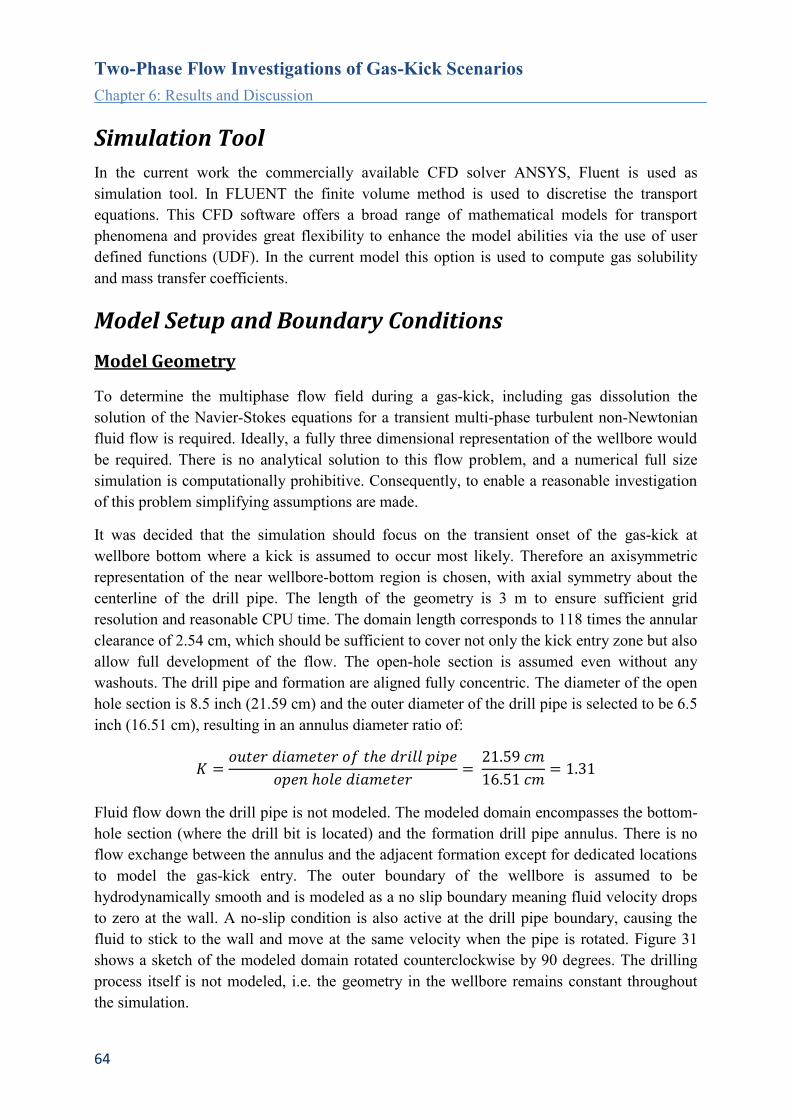
Two-Phase Flow Investigations of Gas-Kick Scenarios
Chapter 6: Results and Discussion
64
Simulation Tool
In the current work the commercially available CFD solver ANSYS, Fluent is used as
simulation tool. In FLUENT the finite volume method is used to discretise the transport
equations. This CFD software offers a broad range of mathematical models for transport
phenomena and provides great flexibility to enhance the model abilities via the use of user
defined functions (UDF). In the current model this option is used to compute gas solubility
and mass transfer coefficients.
Model Setup and Boundary Conditions
Model Geometry
To determine the multiphase flow field during a gas-kick, including gas dissolution the
solution of the Navier-Stokes equations for a transient multi-phase turbulent non-Newtonian
fluid flow is required. Ideally, a fully three dimensional representation of the wellbore would
be required. There is no analytical solution to this flow problem, and a numerical full size
simulation is computationally prohibitive. Consequently, to enable a reasonable investigation
of this problem simplifying assumptions are made.
It was decided that the simulation should focus on the transient onset of the gas-kick at
wellbore bottom where a kick is assumed to occur most likely. Therefore an axisymmetric
representation of the near wellbore-bottom region is chosen, with axial symmetry about the
centerline of the drill pipe. The length of the geometry is 3 m to ensure sufficient grid
resolution and reasonable CPU time. The domain length corresponds to 118 times the annular
clearance of 2.54 cm, which should be sufficient to cover not only the kick entry zone but also
allow full development of the flow. The open-hole section is assumed even without any
washouts. The drill pipe and formation are aligned fully concentric. The diameter of the open
hole section is 8.5 inch (21.59 cm) and the outer diameter of the drill pipe is selected to be 6.5
inch (16.51 cm), resulting in an annulus diameter ratio of:
𝐾 =𝑜𝑢𝑡𝑒𝑟 𝑑𝑖𝑎𝑚𝑒𝑡𝑒𝑟 𝑜𝑓 𝑡ℎ𝑒 𝑑𝑟𝑖𝑙𝑙 𝑝𝑖𝑝𝑒
𝑜𝑝𝑒𝑛 ℎ𝑜𝑙𝑒 𝑑𝑖𝑎𝑚𝑒𝑡𝑒𝑟=
21.59 𝑐𝑚
16.51 𝑐𝑚= 1.31
Fluid flow down the drill pipe is not modeled. The modeled domain encompasses the bottom-
hole section (where the drill bit is located) and the formation drill pipe annulus. There is no
flow exchange between the annulus and the adjacent formation except for dedicated locations
to model the gas-kick entry. The outer boundary of the wellbore is assumed to be
hydrodynamically smooth and is modeled as a no slip boundary meaning fluid velocity drops
to zero at the wall. A no-slip condition is also active at the drill pipe boundary, causing the
fluid to stick to the wall and move at the same velocity when the pipe is rotated. Figure 31
shows a sketch of the modeled domain rotated counterclockwise by 90 degrees. The drilling
process itself is not modeled, i.e. the geometry in the wellbore remains constant throughout
the simulation.

Two-Phase Flow Investigations of Gas-Kick Scenarios
Chapter 5: Modeling Approach
65
Figure 31: Model Setup
Multiphase Flow Model
When carrying out a two-phase flow simulation with FLUENT one has to select the
appropriate multiphase model according to the expected flow pattern, as discussed earlier.
There are different two-phase flow models available according to the size of the phase volume
fraction as well as whether the flow is dispersed or segregated. For instance for a dispersed
flow simulation it is necessary to have knowledge about the bubble or droplet size distribution
a priori. In the present study of a gas-kick such information is not available. As mentioned
earlier it is actually not fully clear what type of flow patterns are evolving.
Therefore the two-phase flow modeling approach adopted for this work is an Euler DNS
based on the volume of fluid method (VOF). Many other modeling approaches need
assumptions that actually constrain the nature of the solution, whereas with the volume of
fluid method no such a priori foundations are needed. The major requirement for a valid
solution is an appropriate selection of the grid resolution to ensure that the fluid interface is
captured properly. Whether the grid resolution fulfills this requirement or not can be validated
by analyzing a histogram of the phase volume fraction. Uniform distribution of phase volume
fractions indicates a smeared phase interface which is a consequence of coarse grid resolution.
Whereas sharp peaks at phase volume fractions close to zero or one indicate good grid
resolution and hence good modeling quality, as can be seen in Figure 32 and Figure 33.
Figure 32: Contour Plot of Gas Volume Fraction
Figure 33: Histogram of Gas Volume
Fraction
With the selection of the volume of fluid method and an appropriate mesh resolution not only
segregated flow can be modeled but also dispersed flow at an arbitrary phase volume fraction,
as long as the mesh size is much smaller than the dispersed interfacial structures. This
approach is well suited to gain information on the arising flow pattern and phase interface
location.
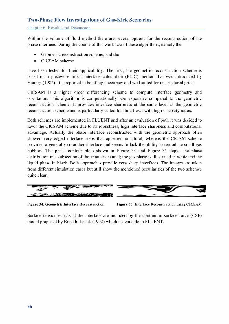
Two-Phase Flow Investigations of Gas-Kick Scenarios
Chapter 6: Results and Discussion
66
Within the volume of fluid method there are several options for the reconstruction of the
phase interface. During the course of this work two of these algorithms, namely the
Geometric reconstruction scheme, and the
CICSAM scheme
have been tested for their applicability. The first, the geometric reconstruction scheme is
based on a piecewise linear interface calculation (PLIC) method that was introduced by
Youngs (1982). It is reported to be of high accuracy and well suited for unstructured grids.
CICSAM is a higher order differencing scheme to compute interface geometry and
orientation. This algorithm is computationally less expensive compared to the geometric
reconstruction scheme. It provides interface sharpness at the same level as the geometric
reconstruction scheme and is particularly suited for fluid flows with high viscosity ratios.
Both schemes are implemented in FLUENT and after an evaluation of both it was decided to
favor the CICSAM scheme due to its robustness, high interface sharpness and computational
advantage. Actually the phase interface reconstructed with the geometric approach often
showed very edged interface steps that appeared unnatural, whereas the CICAM scheme
provided a generally smoother interface and seems to lack the ability to reproduce small gas
bubbles. The phase contour plots shown in Figure 34 and Figure 35 depict the phase
distribution in a subsection of the annular channel; the gas phase is illustrated in white and the
liquid phase in black. Both approaches provide very sharp interfaces. The images are taken
from different simulation cases but still show the mentioned peculiarities of the two schemes
quite clear.
Figure 34: Geometric Interface Reconstruction
Figure 35: Interface Reconstruction using CICSAM
Surface tension effects at the interface are included by the continuum surface force (CSF)
model proposed by Brackbill et al. (1992) which is available in FLUENT.

Two-Phase Flow Investigations of Gas-Kick Scenarios
Chapter 5: Modeling Approach
67
Turbulence Modeling & Grid Considerations
Selection of the mesh has a significant impact on the rate of convergence, solution accuracy
and computational time required. Mesh quality ensuring good numerical accuracy and a
minimum of numerical diffusion is achieved by appropriate grid resolution, low cell
skewness, small size ratio of adjacent cells, an appropriate boundary layer mesh, and local
mesh refinement where needed. In the first modeling step, a grid resolution study has been
conducted. Grid independence of the solution is achieved when an increase in cell number is
not affecting the results. This goal was ultimately met by using quadrilateral cells with a size
of 0,5 mm and certain mesh refinement at gas inlet zones.
Based on the Reynolds number calculated for mere mud circulation, the single phase flow
would be classified as laminar. However due to the entrance of the kick gas turbulences will
arise. Unless a direct numerical simulation with respect to time is planned, an appropriate
turbulence model needs to be selected for the simulation. The realizable k-epsilon model has
proven to be most applicable for this purpose. Fluid flows are significantly affected by the
presence of walls, since this is the location where turbulence is effectively generated. When
using a turbulence model for simulation of the bulk flow special treatment is needed for the
flow in the near-wall region. The near-wall region can be subdivided into three zones with
different characteristics as shown in Figure 36. The parameter y+ is a non-dimensional
distance from the wall, critical in the assessment of mesh quality. It is defined as the shear
velocity times the normal distance from the wall divided by the kinematic viscosity.
𝑦+ =𝑈𝑇𝑦
𝜈, 𝑈𝑇 = √
𝜏𝑤
𝜌
UT shear velocity y normal distance from the wall
The innermost layer of the boundary layer profile is the viscous sublayer next to the wall
which is characterized by laminar flow. In this layer molecular viscosity plays a dominant
role. Then there is the outer fully turbulent layer, where the flow is no more affected by the
presence of the wall. Between these two regimes a buffer layer or blending region is located,
where viscosity and turbulence are equally important.

Two-Phase Flow Investigations of Gas-Kick Scenarios
Chapter 6: Results and Discussion
68
Figure 36: Subdivisions of the Near-Wall Region (FLUENT manual)
To properly capture the boundary layer profile it is necessary to refine the computational grid
accordingly. A considerable amount of additional cells may be required for this task and the
size of these cells imposes a restriction on the size of the time step. Since for an explicit
calculation (transient simulation) the magnitude of the step is governed by the smallest length
scale. So in case of very small computational cells this can lead to extremely small time steps
and increased CPU requirements.
An alternative practice in turbulence modeling is to apply appropriate near wall models to
bridge the low Reynolds flow in the vicinity of the wall with the high Reynolds flow in the
bulk fluid. In this case no local mesh refinement is need. The concept of these two approaches
is shown in Figure 37.
Figure 37: Near-Wall Treatments (FLUENT manual)

Two-Phase Flow Investigations of Gas-Kick Scenarios
Chapter 5: Modeling Approach
69
Regarding the application of wall functions there is a restriction in acceptable y+ values for
the validity of these semi-empirical models. The general criteria requests mesh resolution
fulfilling y+ values of > 15, otherwise the numerical results deteriorate and the accuracy of
the solutions cannot be maintained. This shortcoming was met by the introduction of scalable
wall functions which allow the application of the wall function approach to fine grids with y+
values below 15. This improvement is essential for the current simulation task, since the small
annular clearance of the flow domain and the request to capture the phase interface demands
for a high grid resolution. This high resolution grid would have counter indicated the
application of wall functions due to the small y+ values present. On one hand, to fulfill the y+
criteria of standard wall functions the grid would have needed to be so coarse that the flow
could not be properly captured and on the other hand a further grid refinement required for a
direct numerical simulation was undesirable due to the tremendous CPU requirements. With
the application of scalable wall functions consistent results are produced for grids of arbitrary
refinement. Apart from y+ considerations it is necessary to resolve the boundary layer with at
least 10 cells in the wall normal direction. Therefore the boundary layer mesh needs to be
examined critically and updated if necessary to meet this criterion.
However caution needs to be taken when applying such single-phase wall functions in
multiphase flow. The use of wall functions may be inadequate when several phases exist near
the wall. For instance a high concentration of dispersed phase is present in a continuous phase
layer at the wall. The dispersed phase bubbles could give rise to an additional source of
turbulence which will not be covered by the wall function approach. Due to the lack of
appropriate two-phase wall functions in FLUENT this effect could not be addressed in the
current simulations.
Eventually quadrilateral elements of uniform size were selected to mesh the annulus and
triangle elements are used to model the wellbore bottom including the drill bit section. The
fluid flow in the annulus is mostly aligned with the grid except for the very beginning of the
annulus next to the wellbore bottom, where the flow strongly deviates from the axial
coordinate due to entry effects. The quadrilateral elements have a side length of 0.5 mm. The
overall model contains 400,000 cells.
The realizable k- model combined with the scalable wall functions approach is the
turbulence model used throughout this work. For all calculations the variable time step option
is selected to ensure a Courrant number smaller or equal to 0.25.
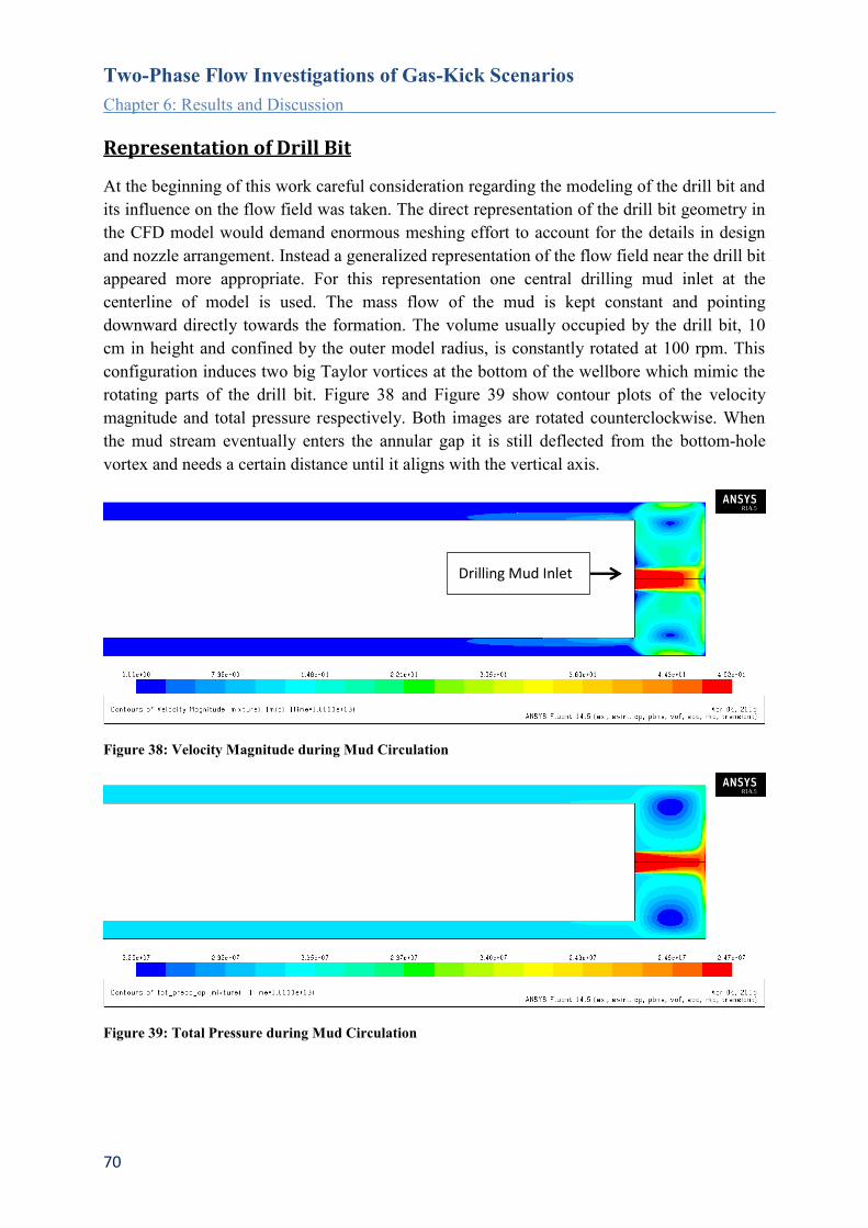
Two-Phase Flow Investigations of Gas-Kick Scenarios
Chapter 6: Results and Discussion
70
Representation of Drill Bit
At the beginning of this work careful consideration regarding the modeling of the drill bit and
its influence on the flow field was taken. The direct representation of the drill bit geometry in
the CFD model would demand enormous meshing effort to account for the details in design
and nozzle arrangement. Instead a generalized representation of the flow field near the drill bit
appeared more appropriate. For this representation one central drilling mud inlet at the
centerline of model is used. The mass flow of the mud is kept constant and pointing
downward directly towards the formation. The volume usually occupied by the drill bit, 10
cm in height and confined by the outer model radius, is constantly rotated at 100 rpm. This
configuration induces two big Taylor vortices at the bottom of the wellbore which mimic the
rotating parts of the drill bit. Figure 38 and Figure 39 show contour plots of the velocity
magnitude and total pressure respectively. Both images are rotated counterclockwise. When
the mud stream eventually enters the annular gap it is still deflected from the bottom-hole
vortex and needs a certain distance until it aligns with the vertical axis.
Figure 38: Velocity Magnitude during Mud Circulation
Figure 39: Total Pressure during Mud Circulation
Drilling Mud Inlet
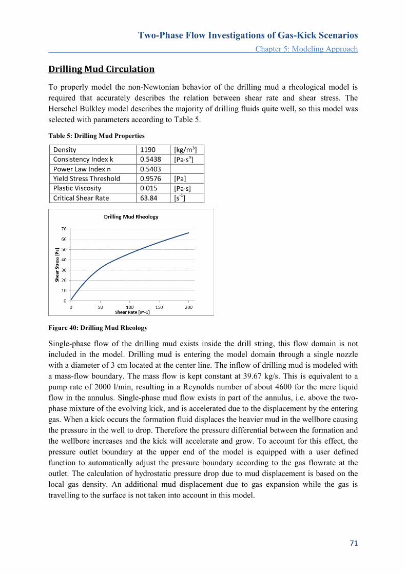
Two-Phase Flow Investigations of Gas-Kick Scenarios
Chapter 5: Modeling Approach
71
Drilling Mud Circulation
To properly model the non-Newtonian behavior of the drilling mud a rheological model is
required that accurately describes the relation between shear rate and shear stress. The
Herschel Bulkley model describes the majority of drilling fluids quite well, so this model was
selected with parameters according to Table 5.
Table 5: Drilling Mud Properties
Density 1190 [kg/m³]
Consistency Index k 0.5438 [Pasn]
Power Law Index n 0.5403
Yield Stress Threshold 0.9576 [Pa]
Plastic Viscosity 0.015 [Pas]
Critical Shear Rate 63.84 [s-1]
Figure 40: Drilling Mud Rheology
Single-phase flow of the drilling mud exists inside the drill string, this flow domain is not
included in the model. Drilling mud is entering the model domain through a single nozzle
with a diameter of 3 cm located at the center line. The inflow of drilling mud is modeled with
a mass-flow boundary. The mass flow is kept constant at 39.67 kg/s. This is equivalent to a
pump rate of 2000 l/min, resulting in a Reynolds number of about 4600 for the mere liquid
flow in the annulus. Single-phase mud flow exists in part of the annulus, i.e. above the two-
phase mixture of the evolving kick, and is accelerated due to the displacement by the entering
gas. When a kick occurs the formation fluid displaces the heavier mud in the wellbore causing
the pressure in the well to drop. Therefore the pressure differential between the formation and
the wellbore increases and the kick will accelerate and grow. To account for this effect, the
pressure outlet boundary at the upper end of the model is equipped with a user defined
function to automatically adjust the pressure boundary according to the gas flowrate at the
outlet. The calculation of hydrostatic pressure drop due to mud displacement is based on the
local gas density. An additional mud displacement due to gas expansion while the gas is
travelling to the surface is not taken into account in this model.

Two-Phase Flow Investigations of Gas-Kick Scenarios
Chapter 6: Results and Discussion
72
Influence of Rotation
Drill pipe rotation is modeled by a moving boundary condition at the inner cylinder and a
rotating fluid zone at the drill bit location. The configuration of an annular flow domain with a
rotating inner cylinder and a stationary outer cylinder quickly reminds one of the well-known
Taylor vortex flow instability. The tendency whether this flow instability is likely to occur in
the current setup, can be assessed by calculating the Taylor number. The Taylor number
characterizes the importance of centrifugal forces due to rotation, relative to viscous forces.
The Taylor number Ta is defined by
𝑇𝑎 =𝑅1Ω1
2𝑑3
𝜈2
where,
R1 radius of the inner cylinder Ω1 angular velocity of the inner cylinder d annular gap between cylinders ν kinematic viscosity
The current setup with a drill-pipe rotation of 100 rpm, an annular gap of 2.5 cm, a radius of
the inner cylinder of 8.26 cm, and a dynamic mud viscosity of ~0.5 Pas results in a Taylor
number of ~800. This is far below the critical Taylor number 3400, which indicates the onset
of the flow instability. This means that even without mud circulation and hence no axial flow
component Taylor-Couette flow vortices are very unlikely to occur inside the annulus. The
vertical flow component will additionally suppress the evolution of radial vortices.
The ratio between the centrifugal force responsible for the Taylor instability and the inertia
force of the axial flow component can be quantified by the Rossby number, defined by
𝑅𝑜 =𝑅1Ω1
𝑗𝐿=
𝑅𝜔
𝑅𝑒
where,
jl axial fluid velocity Rω rotational Reynolds number Re Reynolds number
A Rossby number greater than unity indicates a dominant centrifugal force and consequently
the onset of a Couette flow instability. The Rossby number for the current model setup lies
below 0.4. This means that the axial flow component is much stronger than the radial flow
caused by rotation. The high pumping rate, the small annular gap size, the low rotation rate,
and the high mud viscosity are counteracting the evolution of radial flow. In case a radial flow
component is desired for instance to increase mixing of the phases, these parameters need to
be altered correspondingly.
However in the bottom-hole zone below the drill pipe the critical Taylor number is exceeded
and the formation of Taylor vortices is noticed. As mentioned earlier these vortices are
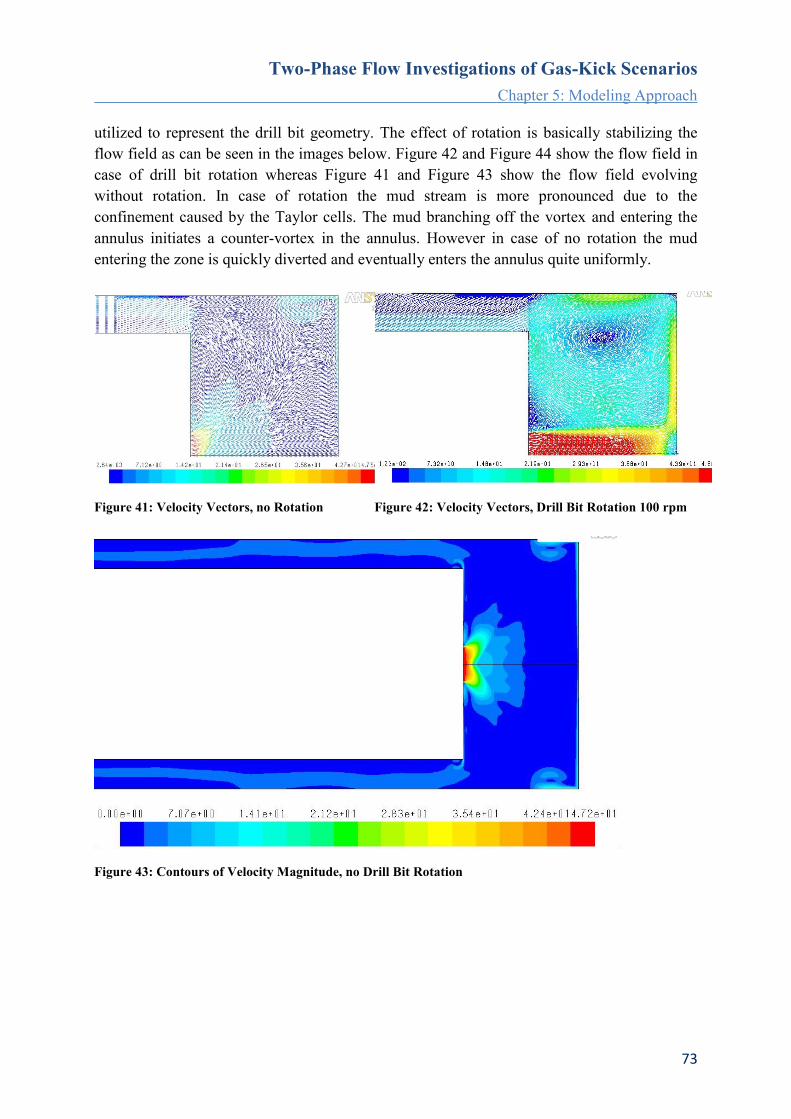
Two-Phase Flow Investigations of Gas-Kick Scenarios
Chapter 5: Modeling Approach
73
utilized to represent the drill bit geometry. The effect of rotation is basically stabilizing the
flow field as can be seen in the images below. Figure 42 and Figure 44 show the flow field in
case of drill bit rotation whereas Figure 41 and Figure 43 show the flow field evolving
without rotation. In case of rotation the mud stream is more pronounced due to the
confinement caused by the Taylor cells. The mud branching off the vortex and entering the
annulus initiates a counter-vortex in the annulus. However in case of no rotation the mud
entering the zone is quickly diverted and eventually enters the annulus quite uniformly.
Figure 41: Velocity Vectors, no Rotation
Figure 42: Velocity Vectors, Drill Bit Rotation 100 rpm
Figure 43: Contours of Velocity Magnitude, no Drill Bit Rotation

Two-Phase Flow Investigations of Gas-Kick Scenarios
Chapter 6: Results and Discussion
74
Figure 44: Contours of Velocity Magnitude, with Drill Bit Rotation 100 rpm
Pressure Situation
The primary cause for a kick to occur is a lower mud pressure than formation pore pressure
especially due to pressure transients. The pressure situation in a wellbore during drilling is
illustrated in Figure 45. The dotted green line shows the static pressure applied by the pumps
at point b, the increase in pressure from b to c is made up by the hydrostatic head of the mud
column minus the frictional pressure losses in the drill string. At the wellbore bottom the drill
bit causes a drop in pressure from point c to d. The pressure drop in the annulus is more
pronounced compared to the pressure drop in the drill string due to the increased frictional
pressure losses in the open-hole section and the flow resistance of the casing shoes. The
formation pore pressure is shown in red and the fracture pressure in blue. During conventional
overbalanced drilling operations the wellbore pressure in the annulus has to be kept inside the
narrow pressure window between the blue and the red line. This circulating mud pressure or
equivalent circulating density (ECD) needed is defined as
𝐸𝐶𝐷 = ℎ𝑦𝑑𝑟𝑜𝑠𝑡𝑎𝑡𝑖𝑐 ℎ𝑒𝑎𝑑 + 𝑓𝑟𝑖𝑐𝑡𝑖𝑜𝑛 𝑝𝑟𝑒𝑠𝑠𝑢𝑟𝑒 + 𝑠𝑢𝑟𝑓𝑎𝑐𝑒 𝑏𝑎𝑐𝑘 𝑝𝑟𝑒𝑠𝑠𝑢𝑟𝑒
The circulating mud pressure in the annulus needs to be larger than the formation pore
pressure to avoid formation fluid influx and lower than the fracture pressure to avoid
fracturing the formation.

Two-Phase Flow Investigations of Gas-Kick Scenarios
Chapter 5: Modeling Approach
75
Figure 45: Wellbore Pressure Situation (taken from http://maris-eu.com)
Formation fluid influx occurs whenever the pressure of a gas-bearing formation exceeds the
pressure in the wellbore. Such pressure differentia can be caused by an unexpected rise in
formation pressure or a decrease in wellbore pressure, possible causes are listed in Table 6.
Table 6: Pressure Situations Causing a Kick
Kick Causes
Reduction in wellbore pressure:
making a connection & stopping
circulation
during tripping
swabbing
lost circulation
low density drilling fluid
gas/oil/water cut
Increase in formation pressure:
unexpected high pressure regions
A rise in formation pressure can be due to geological processes that have occurred in the
region being drilled. Wells are drilled in regions where oil and gas are trapped, and the same
processes that create the hydrocarbons can also produce large pressures. Therefore, it is not
uncommon to come across regions of abnormally high formation pressure while drilling.

Two-Phase Flow Investigations of Gas-Kick Scenarios
Chapter 6: Results and Discussion
76
The mud pressure during circulation is the sum of hydrostatic head of the mud, dynamic head
due to pumping and surface backpressure. Therefore a reduction in wellbore pressure happens
if at least one of these components drops without compensation by another. The hydrostatic
head in the wellbore can drop due to improper well operations. For instance during tripping
when the drill string is pulled from the hole continuous pumping of mud is needed to replace
the volume of the removed pipe with mud. Swabbing can also produce wellbore pressure
drops when done too quickly, especially with high viscosity muds and with small annular
clearance. Low drilling mud density or lost circulation can also cause a reduction in
hydrostatic head. The drilling fluid density may be reduced by the influx of formation fluids
and/or the settling of weighting material. The drilling mud is the well’s primary well barrier,
when the fluid volume is lost to the formation or its pressure is too low the result will be
inflow of formation fluids.
Fraser et al. (2014) have analyzed kick detection data from drilling operations in the Gulf of
Mexico. As a result they identified five main drilling related operations that are estimated to
account for 95% of all kick events in this area, shown in Figure 46. According to their study
about 70% of the kicks occurred when making a connection. When making a connection the
pumps are turned off and the mud pressure level in the wellbore reduces to the hydrostatic
head of the mud column. After a connection is established, circulation is restarted and the
mud pressure in the bore hole rises again rapidly. This transient pressure drop and rise can be
very dramatic and overshooting the balance before stabilizing. The negative pressure surge
may induce flow from the formation if it falls below formation pore pressure. With each
connection the exposed formation is repeatedly depressurized before and supercharged after
the connection is established. According to Fraser et al.’s study such pressure fluctuations in
the wellbore are the main causes for a kick, i.e. tripping out and making a connection sum up
to 85% of the kicks analyzed. With continuous circulation techniques during connection
operations these transient pressure fluctuations can be avoided and the flow is kept steady.
Figure 46: Kick Frequency in Drilling Operations, according to Fraser et al. (2014)

Two-Phase Flow Investigations of Gas-Kick Scenarios
Chapter 5: Modeling Approach
77
Kick-Gas Inlet Condition
When investigating possible scenarios for a gas-kick, with the aim to identify the most
probable location for the kick to enter, one has to analyze the fluid pressure situation in the
wellbore. Usually a gas-kick will occur when drilling into formations with pressures higher
than anticipated and a bottom-hole pressure too small to counteract formation pressure. As
mentioned earlier the hydraulic pressure is making up the major portion of the wellbore
pressure. As the pressure in the wellbore is not uniform, the kick is likely to occur at the
“weakest point” along the wellbore/formation interface.
In general the well is kept under control by using a drilling mud with a density sufficient to
keep the hydrostatic pressure well above formation pore pressure. However when considering
the pressure impact of the moving fluid, it is possible that the flow situation in the wellbore
may cause local zones with a lower pressure than assumed. This is especially true at narrow
flow passages or strong deflections in the flow path. As the passage becomes narrower the
velocity of the mud passing trough will increase and the static fluid pressure will drop, just
similar to the working principle of a Venturi pipe. This drop in static pressure is commonly
used to aerate flows, as shown in Figure 47. The narrow passage of the pipe is used to draw
air into the water stream, basically a kind of “desired gas-kick” situation. Similarly in case the
static wellbore pressure becomes considerably lower than the formation pore pressure, fluid
will be pulled into the wellbore. Such spots of low static pressure can cause a continuous
inflow of small amounts of gas. This inflow may not threat overall well control but can have a
considerable impact on the drilling string in terms of corrosion.
Figure 47: Venturi Aerator
Figure 48 shows the total pressure, i.e. sum of static and dynamic pressure, in the wellbore
model during mud circulation. The pressure range is clipped; the gradual hydrostatic pressure
increase can clearly be seen as well as the high dynamic pressure regions due to the flow in
the drill bit area.
Figure 48: Total Pressure [Pa] during Mud Circulation
z-direction
Air Suction
Water Flow
Water + Air Flow
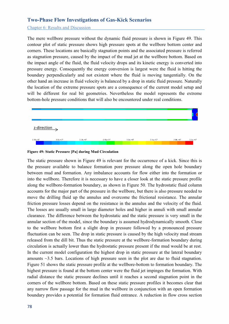
Two-Phase Flow Investigations of Gas-Kick Scenarios
Chapter 6: Results and Discussion
78
The mere wellbore pressure without the dynamic fluid pressure is shown in Figure 49. This
contour plot of static pressure shows high pressure spots at the wellbore bottom center and
corners. These locations are basically stagnation points and the associated pressure is referred
as stagnation pressure, caused by the impact of the mud jet at the wellbore bottom. Based on
the impact angle of the fluid, the fluid velocity drops and its kinetic energy is converted into
pressure energy. Consequently the energy conversion is largest were the fluid is hitting the
boundary perpendicularly and not existent where the fluid is moving tangentially. On the
other hand an increase in fluid velocity is balanced by a drop in static fluid pressure. Naturally
the location of the extreme pressure spots are a consequence of the current model setup and
will be different for real bit geometries. Nevertheless the model represents the extreme
bottom-hole pressure conditions that will also be encountered under real conditions.
Figure 49: Static Pressure [Pa] during Mud Circulation
The static pressure shown in Figure 49 is relevant for the occurrence of a kick. Since this is
the pressure available to balance formation pore pressure along the open hole boundary
between mud and formation. Any imbalance accounts for flow either into the formation or
into the wellbore. Therefore it is necessary to have a closer look at the static pressure profile
along the wellbore-formation boundary, as shown in Figure 50. The hydrostatic fluid column
accounts for the major part of the pressure in the wellbore, but there is also pressure needed to
move the drilling fluid up the annulus and overcome the frictional resistance. The annular
friction pressure losses depend on the resistance in the annulus and the velocity of the fluid.
The losses are usually small in large diameter holes and higher in annuli with small annular
clearance. The difference between the hydrostatic and the static pressure is very small in the
annular section of the model, since the boundary is assumed hydrodynamically smooth. Close
to the wellbore bottom first a slight drop in pressure followed by a pronounced pressure
fluctuation can be seen. The drop in static pressure is caused by the high velocity mud stream
released from the dill bit. Thus the static pressure at the wellbore-formation boundary during
circulation is actually lower than the hydrostatic pressure present if the mud would be at rest.
In the current model configuration the highest drop in static pressure at the lateral boundary
amounts ~3.5 bars. Locations of high pressure seen in the plot are due to fluid stagnation.
Figure 51 shows the static pressure profile at the wellbore-bottom to formation boundary. The
highest pressure is found at the bottom center were the fluid jet impinges the formation. With
radial distance the static pressure declines until it reaches a second stagnation point in the
corners of the wellbore bottom. Based on these static pressure profiles it becomes clear that
any narrow flow passage for the mud in the wellbore in conjunction with an open formation
boundary provides a potential for formation fluid entrance. A reduction in flow cross section
z-direction

Two-Phase Flow Investigations of Gas-Kick Scenarios
Chapter 5: Modeling Approach
79
can be a matter of wellbore design but also be due to clogging. Shutting in a well helps to
reestablish a known pressure situation i.e. hydrostatic pressure.
Figure 50: Static Pressure Profile along Lateral Boundary, during Mud Circulation
Figure 51: Static Pressure Profile along Bottom-Hole Boundary, during Mud Circulation
When looking at the pressure situation during mud circulation, we can classify three distinct
pressure sections along the wellbore model boundary. These sections are illustrated in Figure
50 in green, red and blue and are described below.
z-direction

Two-Phase Flow Investigations of Gas-Kick Scenarios
Chapter 6: Results and Discussion
80
The wellbore bottom or drill bit area (indicated in blue), defined as the volume below the
annular channel. In this section the drill bit itself is located. Although the drill bit is not
explicitly modeled in the model it is clear that the high velocity of the drilling mud leaving the
drill bit nozzles and the limited space left between drill bit and formation is resulting in a
highly fluctuating static pressure profile along the boundary. Depending on the angle of flow
impact and velocity there are high pressure stagnation points and sections of low static
pressure.
The transition zone, characterized by strong entry effects (indicated in red). This section is
located at the beginning of the annular channel right above the drill bit. At this entry point of
the drilling mud into the wellbore annulus we can see strong entry effects due to the change in
geometry. The fluid path lines are strongly deflected and a pressure drop can be seen at the
formation-wellbore boundary.
The annular channel above the transition zone, indicated in green. In this section a stable and
continuous flow field over the whole annular cross section has established. No effects from
the fluid entry point can be seen. The static pressure at the wellbore boundary shows a gradual
profile dominated by the hydrostatic pressure. The pressure situation in this section
corresponds to what is commonly expected in wellbore analysis. The flow has become
unidirectional and can be computed based on the Hagen-Poiseuille equation.
To better illustrate the conditions at wellbore bottom, Figure 52 to Figure 54 show a zoomed
in view of the static pressure distribution and velocity field. In the first image the motion of
the fluid is illustrated with pathlines to better illustrate the evolving fluid vortices. The
pressure scale is clipped to a range of 233 to 234 bars. A recirculation zone can be identified
right at the beginning of the annulus. This vortex is a consequence of the deflected entry of
the mud stream into the annulus caused by drill bit rotation. As the velocity vectors are
indicating fluid is actually flowing backwards along the outer boundary. This vortex can be of
special interest regarding phase mixing. Another stagnation point can be seen where the mud
stream hits the drill pipe. Of course the shown flow field is a consequence of model
configuration. But whatever drill bit configuration is used there will always be strong entry
effects until the mud adopts a velocity profile aligned with the annulus.
Figure 52: Static Pressure [Pa] and Flow Pathlines
z-direction

Two-Phase Flow Investigations of Gas-Kick Scenarios
Chapter 5: Modeling Approach
81
Figure 53: Static Pressure [Pa] and Velocity Vectors
Figure 54: Velocity Magnitude [m/s]
The bottom-hole and transition zone represent the locations with the lowest static pressure
counteracting the formation pore pressure. In case the pressure situation becomes
underbalanced, the pressure gradient between formation and wellbore will be largest at these
zones making them the most probable spots for formation fluid inflow, according to the
current configuration.
For the simulation of the gas-kick the flow in the wellbore model is first calculated based on
mere mud circulation to approach steady state conditions. This solution provides the initial
condition before the kick gas is introduced. Several geometric scenarios for the gas-kick entry
are investigated and illustrated in the result section of this thesis. For most simulation cases
the boundary condition for the gas inlet is a constant pressure boundary. This boundary
condition is realistic on the short time, since the pressure in the reservoir will not be affected
by the gas escaping into the wellbore. There are also a few simulation cases where the gas is
assumed to enter at a constant mass flow rate. The mass flow boundary condition basically
skips the transient onset of gas inflow and reflects an uncontrolled kick situation.
z-direction
z-direction
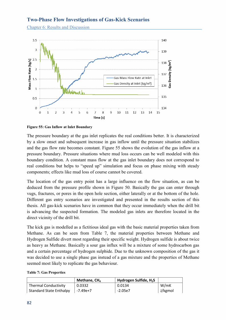
Two-Phase Flow Investigations of Gas-Kick Scenarios
Chapter 6: Results and Discussion
82
Figure 55: Gas Inflow at Inlet Boundary
The pressure boundary at the gas inlet replicates the real conditions better. It is characterized
by a slow onset and subsequent increase in gas inflow until the pressure situation stabilizes
and the gas flow rate becomes constant. Figure 55 shows the evolution of the gas inflow at a
pressure boundary. Pressure situations where mud loss occurs can be well modeled with this
boundary condition. A constant mass flow at the gas inlet boundary does not correspond to
real conditions but helps to “speed up” simulation and focus on phase mixing with steady
components; effects like mud loss of course cannot be covered.
The location of the gas entry point has a large influence on the flow situation, as can be
deduced from the pressure profile shown in Figure 50. Basically the gas can enter through
vugs, fractures, or pores in the open hole section, either laterally or at the bottom of the hole.
Different gas entry scenarios are investigated and presented in the results section of this
thesis. All gas-kick scenarios have in common that they occur immediately when the drill bit
is advancing the suspected formation. The modeled gas inlets are therefore located in the
direct vicinity of the drill bit.
The kick gas is modelled as a fictitious ideal gas with the basic material properties taken from
Methane. As can be seen from Table 7, the material properties between Methane and
Hydrogen Sulfide divert most regarding their specific weight. Hydrogen sulfide is about twice
as heavy as Methane. Basically a sour gas influx will be a mixture of some hydrocarbon gas
and a certain percentage of hydrogen sulphide. Due to the unknown composition of the gas it
was decided to use a single phase gas instead of a gas mixture and the properties of Methane
seemed most likely to replicate the gas behaviour.
Table 7: Gas Properties
Methane, CH4 Hydrogen Sulfide, H2S
Thermal Conductivity 0.0332 0.0134 W/mK Standard State Enthalpy -7.49e+7 -2.05e7 J/kgmol

Two-Phase Flow Investigations of Gas-Kick Scenarios
Chapter 5: Modeling Approach
83
Molecular Weight 16.04 34.08 kg/kgmol Specific Heat, cp 2222 2222 J/kgK Viscosity 1.087e-5 1.2e-5 kg/ms
Reference Temperature 298 K
Modeling of Gas Dissolution
In view of the fact that gas dissolution in drilling mud systems is an essential sub-process
initiating corrosion, developing an understanding on the conditions enhancing or retarding mass
transfer for this process is critical. In order to apply the concept of mass transfer rate
calculation to the situation of gas influx in a wellbore, the mass transfer coefficient is a crucial
parameter that needs to be chosen appropriately to reflect the unsteady flow situation of a kick
event. The flow situation during a kick in the near drill bit section is dominated by the sudden
inflow of formation fluid and expected to cause rapid mixing of the drilling mud and kick gas
thereby enhancing the gas-liquid mass transfer.
Within the computational model the process of gas dissolution and release is modeled as mass
transfer interaction between the gas and the liquid phase. Modeling mass transfer with the
CFD solver FLUENT requires the input of a mass transfer rate per unit volume as interaction
parameter between two phases. This can be done by either specifying a constant value, or
selecting one of the built in models for mass transfer, or by defining a user defined function
(UDF) for the computation of the mass transfer rate. In this work the latter approach has been
chosen. With the means of a user defined function the volumetric mass transfer rate for each
computational cell is calculated and updated at every time step. Based on the computed mass
transfer rate FLUENT then adds contributions to the mass, species, and energy equations.
As mentioned earlier in this work the mass transfer rate can be defined as
𝑑𝑚
𝑑𝑡= 𝑘𝑀𝐴(𝐶𝑆 − 𝐶0)
where
m mass [kg] k mass transfer coefficient [m/s] M molecular weight of gas [kg/mole] A interface area [m²] CS gas solubility [mole/m³] C0 concentration of dissolved gas [mole/m³]
Precise knowledge of the gas-liquid interface area is needed for calculation of the mass
transfer rate. The size of the interface area has probably a stronger influence on the computed
mass transfer rate than the selection of the mass transfer coefficient, especially in dispersed
flow. The problem with the interface area is that it can neither be properly measured
experimentally nor can it be exactly determined within a CFD simulation.
Dividing the above definition with the cell volume provides the requested mass transfer rate
input for the simulation.

Two-Phase Flow Investigations of Gas-Kick Scenarios
Chapter 6: Results and Discussion
84
𝑔𝑙 = 𝑘𝑀𝐴
𝑉(𝐶𝑆 − 𝐶0)
𝑔𝑙 mass transfer rate, from gas to liquid phase [kg/m³s]
Based on this equation the cell based phase interface area per volume is needed. For this task
a user defined function was set up and the computed interface area was stored in a user
defined memory. Figure 56 shows a typical contour plot of phase distribution in the lower
third of the wellbore model, the mud is indicated in black and the gas in white. The calculated
interface area per volume is shown in Figure 57.
Figure 56: Phase Distribution
Figure 57: Computed Interface Area per Volume [m²/m³]
However difficulties arose when trying to update the computed interface area per cell with
each time step. Unfortunately no straightforward solution was found to continuously update
this value due to peculiarities of the simulation tool. An alternative approach was found by
replacing the specific interface area 𝐴
𝑉 with a term containing the gradient of the phase
indicator function. This term basically represents the interface area density and is defined for
the asymmetrical case as
𝐴
𝑉 ∝ 𝑉𝑂𝐹𝑔𝑟𝑎𝑑 = √(
𝑑𝑓
𝑑𝑥)
2
+ (𝑑𝑓
𝑑𝑦)
2
VOFgrad volume fraction gradient f phase indicator function
This term can easily be calculated and continuously updated with means of a user defined
function. Figure 58 shows a contour plot of volume fraction gradient term that is consequently
used to compute the mass transfer rate. It can be seen that the interface is captured quite well
and that there is a good correlation with the specific interface area plot.
z-direction
z-direction

Two-Phase Flow Investigations of Gas-Kick Scenarios
Chapter 5: Modeling Approach
85
Figure 58: Contours of Volume Fraction Gradient [m-1
]
The computed volume fraction gradient is generally lower than the computed specific
interface area shown in Figure 57. The values differ by a factor ~2.5, probably originating
from cell geometry. To fit the volume fraction gradient term to the specific interface area
proportionality constant is introduced.
𝐴
𝑉= 2.5 𝑉𝑂𝐹𝑔𝑟𝑎𝑑
Figure 59: Contours of Volume Fraction Gradient Times Proportionality Constant [m-1
]
The mass transfer coefficient k needed for the computation of the volumetric mass transfer
rate is calculated using a Sherwood correlation. As mentioned earlier Sherwood correlations,
used to define mass transfer coefficients, are describing the mass transfer process of an overall
process. Nevertheless calculation of mass transfer coefficients for use in a numerical model
can be done with the help of a Sherwood correlation, if the correlation is based on local
parameters utilizing the detailed information on the flow field provided by the CFD
simulation. This approach leads to local mass transfer coefficients feeding the computation of
a local mass transfer rates. Multiplication of local mass transfer coefficient times the local
interfacial area and integration throughout the model domain will give the overall volumetric
mass transfer coefficient of the system. The mass transfer coefficient used in a CFD
simulation is influenced by the degree of the model’s grid resolution, and consequently to
what extent the mass transfer coefficient has to incorporate missing information on the
interface area. A high grid resolution provides more detailed information on the phase
interface and its morphology whereas a coarse grid resolution underestimates the phase
interface area and its shape effect on the mass transfer process. This difficulty is often
addressed by combining mass transfer coefficient and interface area to a volumetric mass
transfer coefficient, which is also easier to compare with experimentally obtained data.
z-direction
z-direction
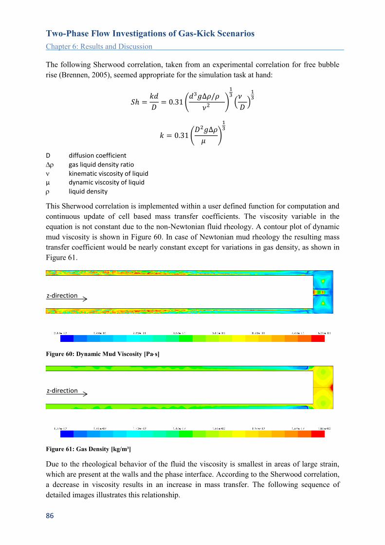
Two-Phase Flow Investigations of Gas-Kick Scenarios
Chapter 6: Results and Discussion
86
The following Sherwood correlation, taken from an experimental correlation for free bubble
rise (Brennen, 2005), seemed appropriate for the simulation task at hand:
𝑆ℎ =𝑘𝑑
𝐷= 0.31 (
𝑑3𝑔∆𝜌/𝜌
𝜈2 )
13
(𝜈
𝐷)
13
𝑘 = 0.31 (𝐷2𝑔∆𝜌
𝜇)
13
D diffusion coefficient
gas liquid density ratio
kinematic viscosity of liquid µ dynamic viscosity of liquid
liquid density
This Sherwood correlation is implemented within a user defined function for computation and
continuous update of cell based mass transfer coefficients. The viscosity variable in the
equation is not constant due to the non-Newtonian fluid rheology. A contour plot of dynamic
mud viscosity is shown in Figure 60. In case of Newtonian mud rheology the resulting mass
transfer coefficient would be nearly constant except for variations in gas density, as shown in
Figure 61.
Figure 60: Dynamic Mud Viscosity [Pas]
Figure 61: Gas Density [kg/m³]
Due to the rheological behavior of the fluid the viscosity is smallest in areas of large strain,
which are present at the walls and the phase interface. According to the Sherwood correlation,
a decrease in viscosity results in an increase in mass transfer. The following sequence of
detailed images illustrates this relationship.
z-direction
z-direction

Two-Phase Flow Investigations of Gas-Kick Scenarios
Chapter 5: Modeling Approach
87
Figure 62: Phase Distribution, Mud [black], Gas [white]
Figure 63: Strain Rate [s-1
]
Figure 64: Mud Viscosity [Pas]
Figure 65: Mass Transfer Coefficient [m/s]
The diffusion coefficient basically depends on temperature, liquid viscosity, and molecule
radius. Since diffusion is not playing a dominant role in the event of a gas-kick, a constant
diffusion coefficient of 1.7e-9 m²/s is applied in the current model.
The computed mass transfer coefficients based on the above Sherwood correlation are shown
in Figure 66. As already mentioned the spatial variation of mass transfer coefficient is mainly
a function of the molecular viscosity used for the computation. The highest values can be
found at the gas jet entry, along the phase interface, and in the drill bit area, see also the phase
distribution shown in Figure 56.

Two-Phase Flow Investigations of Gas-Kick Scenarios
Chapter 6: Results and Discussion
88
Figure 66: Mass Transfer Coefficient [m/s], based on Sherwood Correlation
For comparison reasons the mass transfer coefficient based on the surface renewal model of
Kataoka and Miyauchi (1969), taking into account the turbulent dissipation rate , is shown in
Figure 67. The underlying equation is defined as
𝑘 = 0.5 (휀
𝜈)
14
𝐷12
Figure 67: Mass Transfer Coefficient [m/s], based on Kataoka and Miyauchi (1969)
The mass transfer coefficients computed based on the Kataoka and Miyauchi (1969) model
are 10 to 20 times higher and show a much wider range compared to the Sherwood correlation
based values. The turbulence based model shows generally high values in the drill bit area and
values are dropping quickly along the annulus, where the values show a similar spatial
distribution like the Sherwood based values. The Sherwood correlation based values are
locally prominent at the phase interface. The shear thinning behavior of the mud is basically
favoring mass transfer. In the Kataoka and Miyauchi model this effect due to viscosity is
overlapped with the contribution of wherever high turbulent dissipation occurs.
After having discussed the definition of the interface area term and the mass transfer
coefficient, specification of molecular weight and gas solubility are left to complete the
computation of mass transfer rate. The molecular weight of hydrogen sulfide amounts 34.08
g/mol. Gas solubility is calculated based on a fit approximating the results of the
thermodynamic model for H2S solubility in pure water of Duan et al. (2007). The fit is
intentionally overestimating the model results, since it is assumed that H2S will be more
soluble in water based mud compared to pure water. This approximation seems to be a
reasonable approach in view of the fact that no experimental data or model for H2S solubility
z-direction
z-direction

Two-Phase Flow Investigations of Gas-Kick Scenarios
Chapter 5: Modeling Approach
89
in water based mud could be found. The calculation of gas solubility is implemented via a
user defined function and computed values are illustrated in Figure 68.
Figure 68: Gas Solubility [mol/m³]
The gas dissolved in the mud is assumed to remain molecular; no dissociation stages of
hydrogen sulfide in the aqueous mud are covered. This assumption is valid for pH values
below 6. At higher pH values H2S tends to reversibly dissociate in two stages depending on
pH. To account for a change in mud properties due to dissolved gas, the mud is modeled as a
mixture and the properties are updated based on a mixing law. In the current simulation cases
the amount of dissolved gas is so small that the change in mud properties is negligible.
The difference between gas solubility and dissolved gas provides the last term needed for the
computation of mass transfer rate. A typical contour plot of mass transfer rate is shown in
Figure 69.
Figure 69: Mass Transfer Rate [kg/m³s]
Apart from calculation of volumetric mass transfer rates for gas dissolution, the user defined
function constantly evaluates the conditions whether gas may come out of solution. Based on
the local solubility gas is allowed to escape from solution when the local dissolved gas
concentration exceeds this value. The release rate is computed similarly like the dissolution
rate, using the reciprocal of the characteristic cell length l instead of the interface area density.
𝑙𝑔 = −𝐾𝑀1
𝑙(𝐶0 − 𝐶𝑆)
𝑙𝑔 mass transfer rate, from liquid to gas phase [kg/m³s]

Two-Phase Flow Investigations of Gas-Kick Scenarios
Chapter 6: Results and Discussion
90
6. Results and Discussion
This section of the thesis is structured into two parts. The first part discusses methods of data
analysis and interpretation of two phase flow. In the second part results of different kick
scenarios are presented.
Quantification of Two Phase Flow
When setting up a simulation case for a multiphase flow problem, apart from considerations
regarding the model setup along with boundary and initial conditions, one has to decide on
how results can be evaluated, what quantities are characteristic and where and how they
should be observed. Especially for a transient simulation a clear understanding of the flow
problem in advance is needed in order to specify the proper quantities for monitoring during
the course of computation.
Historically the most common parameters used in the 1-dimensional analysis of two-phase
flow are:
Void fraction or liquid holdup
Prediction of the void fraction is indispensable for the analysis of two-phase flow. It is
the dominant parameter for processes involving mass transfer and chemical reactions.
Superficial phase velocity
It is defined as the volume flux divided by the total cross-sectional area of the tube and
often used as parameter in flow pattern maps.
Slip ratio Ug/Ul
Originating from the drift flux modeling approach the velocity ratio between the gas
and liquid phase is often used to characterize two-phase flow.
With the extensive data available from a transient CFD simulation the list of characteristic
flow parameters may be extended by parameters reflecting the flow variations in time and
space. Similar to common evaluation practice of unsteady flow experiments it appears equally
adequate for unsteady flow simulations to measure the fluctuating flow quantities at
representative locations of the modeled domain. These variations are best illustrated by the
means of histograms or distributions and corresponding statistical parameters. Some
parameters like for instance the phase interface area cannot be measured directly but instead
only interpreted based on volume fraction information of the flow field. Additionally, integral
parameters obtained on representative surfaces, cross sections, and volumes complete the list
of result parameters. Using such techniques helps to summarize the amount of data available
from a CFD simulation. This is necessary since a mere visual inspection is very difficult due
to the elongated model geometry. The overall goal is to compress and extract key information
that helps to ease the comparison between simulation cases.

Two-Phase Flow Investigations of Gas-Kick Scenarios
Chapter 6: Results and Discussion
91
Velocity Data
In a CFD simulation using the volume of fluid method to model two phase flow the resulting
velocity field is shared by both phases. However with the help of a high grid resolution it is
possible to dedicate mixture velocity to a single phase in cells fully occupied with one fluid.
Another useful method to characterize the flow based on velocity data is to look at the spatial
variations of mixture velocity within the flow channel. Therefore histograms of axial and
radial velocity components are used. Using time averaged mean velocity values the histogram
can be seen as an estimate of the probability distribution of axial velocity. Time averaging can
be done after the flow has become stable, indicated by the mass balance at the model
boundaries.
Figure 70: Histogram of Axial Mixture Velocity in
the Annular Channel
Figure 71: Histogram of Radial Mixture Velocity in
the Annular Channel
Figure 70 shows the histogram of axial velocity of four simulated kick scenarios. Negative
velocity accounts for upward flow, any positive values indicate reverse flow in the annular
channel. The series denoted LFK_1 shows the broadest range of axial velocities and BHFK_1
has the narrowest axial velocity distribution. The magnitude of radial fluid movement can be
judged by the radial velocity distribution shown in Figure 71.
The broad axial velocity distribution of LFK_1 is a result of the following flow situation:
Right after the location of gas inflow there is a clear phase separation and phase velocities
differ by a factor of two. After a distance of 30 times the annular clearance the velocities of
both phases have equalized and phases are still clearly separated. From there on the phase
interface starts to deteriorate more and more and the gas phase accelerates. The phase
interface changes from small ripples, to large waves that eventually break up and produce
numerous fluid ligaments and droplets. With increasing distance from the gas inlet the
velocity of the gas phase increases and the velocity of the mud phase decreases. No notable
flow recirculation can be found in this case.
The narrowest axial velocity distribution belongs to the simulation case BHFK_1. In this case
gas and mud show hardly any difference in axial velocity. The flow morphology has
characteristics of both bubble flow and churn flow. Elongated fluid ligaments can be found

Two-Phase Flow Investigations of Gas-Kick Scenarios
Chapter 6: Results and Discussion
92
near the annular walls and larger bubbles travelling in the core of the annulus. The fluid
ligaments are actually a wake of small gas bubbles smeared of from the periodic generation of
Taylor bubbles at the entrance to the annular channel. The bubbles traveling in the core have a
size of approximately a third of the annular clearance and show the typical tail-dented shape
of Taylor bubbles. Due to the limited variation in axial velocity, the shape of the fluid
structures stays nearly constant after a distance of 30 times the annular clearance. The
rotational component in the flow is clearly indicated by the broader distribution of radial
mixture velocities shown in Figure 71.
Simulation case LFK_2 shows similar behavior like LFK_1. Velocities are lower since the
differential pressure applied at the gas inlet is about seven times smaller. The shape of the
axial velocity distributions is comparable. However in LFK_2 not only the inner cylinder is
rotated but also the whole annular channel is rotated. This setup was chosen to mimic the
influence of near drill bit assembly like stabilizers that impose additional rotational drag
compared to a smooth pipe. The annular rotation causes a narrow radial velocity distribution
as can be seen in Figure 71, as the exchange between fluid layers is limited. As a consequence
the shape of the phase interface is very smooth.
The other extreme of radial velocity distribution belongs to simulation case LFK_0D. Here
strong radial momentum exchange between the phases occurs, resulting in a very complex
phase distribution and increased phase interface area. The bubble flow regime of BHFK_1
shows limited radial fluid movement. It is the breakup of annular flow and its transformation
into wispy annular, and slug/churn flow regime types that show the broadest radial velocity
distribution. This may also explain why flow regimes like churn and slug show the highest
fluid mechanical damage on pipe walls observed in experiments.
To summarize, the histograms of radial and axial velocities in the annular channel help to
identify the existence of flow recirculation cells. The profiles show typical shapes according
to flow regime. Thereby it is possible to identify flow patterns based on measureable
parameters instead of visual inspection. The data has to be collected when the flow in the
simulated channel section has stabilized. Consequently the illustrations provide no
information on the temporal evolution of the flow.
The flow morphology i.e. phase distribution of the simulation cases discussed is illustrated in
Figure 73 to Figure 76. Figure 72 shows the length of 30 times the annular clearance
measured upwards from the annular entrance.
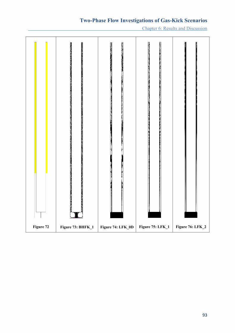
Two-Phase Flow Investigations of Gas-Kick Scenarios
Chapter 6: Results and Discussion
93
Figure 72
Figure 73: BHFK_1
Figure 74: LFK_0D
Figure 75: LFK_1
Figure 76: LFK_2

Two-Phase Flow Investigations of Gas-Kick Scenarios
Chapter 6: Results and Discussion
94
Void fraction
Void fraction is often used as an indicator for the transition from bubbly flow to slug flow.
For instance Taitel et al. (1980) suggest that for bubbles of uniform size in flowing in a pipe,
the transition occurs when the gas void fraction reaches 0.25. Caetano et al. (1992) observed
this transition at an average void fraction of 0.2 in a concentric annulus. They observed an
even earlier transition at a void fraction of 0.15 for flow through a fully eccentric annulus.
Apparently the gap size has a strong influence on the change from a bubbly to a slug flow
pattern. It is the influence of the channel walls on the velocity profile of the flow that
increases the collision rate of the gas bubbles leading to the formation of slugs.
An increase in gas flow rate destructs the initial slug flow resulting in a churning and
oscillatory flow situation. Eventually at very high gas flow rates, the flow becomes annular
with a liquid film on the walls and a gas continuum in the annular core. These changes will be
illustrated via averaged void fraction profiles along the annulus in the next section of this
work.
Another characteristic that is useful in classifying flow patterns is the level of intermittency in
the volume fraction. Examples of strong intermittent flow patterns are slug flows and the
occurrence of interfacial waves in separated flow. With the analysis of time series of
dedicated flow quantities in the frequency domain information about flow fluctuations can be
provided. For instance slug frequency can be obtained from the time series of void fraction.
Furthermore geometric information on flow structures can be obtained with this technique. An
example will be shown in the next section of this thesis.
Finally a histogram of void fraction is very helpful to evaluate whether the model’s grid
resolution is adequate to capture the two-phase flow morphology of the current setting. It
serves as a measure of quality for the applied modeling approach. Figure 77 shows histograms
of gas void fraction of selected simulation cases. Basically all simulation cases show a good
phase separation and low smearing, indicating that the grid resolution is adequate to resolve
the occurring flow structures. For case BHFK_1 the grid resolution is becoming critical to
capture the small bubbles occurring in this simulation, but the overall coverage of the flow is
still good.

Two-Phase Flow Investigations of Gas-Kick Scenarios
Chapter 6: Results and Discussion
95
Figure 77: Histograms of Gas Volume Fraction
Simulated Kick Scenarios
In this section selected simulation cases are presented and discussed.
The manifestation of a kick basically depends on the following parameters:
Overall depth (pressure, temperature)
Annular geometry (annular clearance)
Drilling mud properties (density, rheology, mud type)
Operational conditions (circulation, shut in)
Location and configuration of kick entrance
Differential pressure between the wellbore and the formation
With respect to this parameter list the first four parameters are kept constant in the presented
simulation cases. The latter two parameters are varied and their influence will be shown. The
boundary conditions for the simulation cases are chosen to reproduce steady-state flow
regimes ranging from bubble flow to annular flow, classified as:
Dispersed flow (bubble flow)
Intermittent flow (churn flow)
Separated flow (annular flow)
The positioning of the presented simulation cases is illustrated in the flow regime map of
Caetano (1992) for concentric vertical annuli in Figure 78. Due to the constant mud flow rate
applied to all simulation cases the values are aligned along one line.

Two-Phase Flow Investigations of Gas-Kick Scenarios
Chapter 6: Results and Discussion
96
Figure 78: Flow Regime Map Illustrating the Range of Simulation Cases
The first group of simulation cases presented in this chapter is focusing on the location of kick
entrance. The major parameters for each kick scenario are listed and a sketch is illustrating the
inlet configuration of the kick gas. A detailed analysis of the occurring flow phenomena is
given including the assessment of specific phase interface area and gas dissolution
parameters. The second group of discussed simulation cases is investigating kick scenarios
leading to a loss of mud circulation.
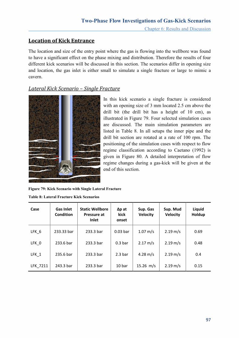
Two-Phase Flow Investigations of Gas-Kick Scenarios
Chapter 6: Results and Discussion
97
Location of Kick Entrance
The location and size of the entry point where the gas is flowing into the wellbore was found
to have a significant effect on the phase mixing and distribution. Therefore the results of four
different kick scenarios will be discussed in this section. The scenarios differ in opening size
and location, the gas inlet is either small to simulate a single fracture or large to mimic a
cavern.
Lateral Kick Scenario – Single Fracture
In this kick scenario a single fracture is considered
with an opening size of 3 mm located 2.5 cm above the
drill bit (the drill bit has a height of 10 cm), as
illustrated in Figure 79. Four selected simulation cases
are discussed. The main simulation parameters are
listed in Table 8. In all setups the inner pipe and the
drill bit section are rotated at a rate of 100 rpm. The
positioning of the simulation cases with respect to flow
regime classification according to Caetano (1992) is
given in Figure 80. A detailed interpretation of flow
regime changes during a gas-kick will be given at the
end of this section.
Table 8: Lateral Fracture Kick Scenarios
Case Gas Inlet Condition
Static Wellbore Pressure at
Inlet
∆p at kick
onset
Sup. Gas Velocity
Sup. Mud Velocity
Liquid Holdup
LFK_6 233.33 bar 233.3 bar 0.03 bar 1.07 m/s 2.19 m/s 0.69
LFK_0 233.6 bar 233.3 bar 0.3 bar 2.17 m/s 2.19 m/s 0.48
LFK_1 235.6 bar 233.3 bar 2.3 bar 4.28 m/s 2.19 m/s 0.4
LFK_7211 243.3 bar 233.3 bar 10 bar 15.26 m/s 2.19 m/s 0.15
Figure 79: Kick Scenario with Single Lateral Fracture

Two-Phase Flow Investigations of Gas-Kick Scenarios
Chapter 6: Results and Discussion
98
Figure 80: Flow Pattern Map for Concentric Annuli, Caetano (1992)
For all simulation cases the gas inflow is comparable to a jet impinging perpendicularly on the
continuous mud flow in the annulus. The available cross sectional area for the mud passage is
reduced dramatically causing an increase in mud velocity. This results in a configuration of a
mud jet pointing upwards and laterally impinged by the gas jet.
Which one of two fluids is forming the dominant jet depends on the ratio of the driving
pressure differential per fluid. The driving pressure differential for the gas is defined by
formation pressure and wellbore pressure at the entry point, for the liquid it is the pressure
gradient in the wellbore produced by the pump. In the CFD simulations the inflow of the
drilling mud is specified as a constant mass flow rate at all times and the formation pressure is
modeled by a constant inflow pressure boundary for the gas. Naturally the pressure in the
wellbore will change due to the inflow of the gas and continuously alter the flow situation
until both fluids are in balance.
A close-up view of the channel including the gas inlet is shown in Figure 81 to Figure 84. The
images belong to simulation case LFK_1. The pressure situation before and during the gas-
kick is illustrated, as well as the velocity field, kinetic energy and phase distribution. The
intruding gas is forcing the mud to move as a thin film along the inner cylinder at increased
speed. Immediately above and below the gas jet a zone of lower pressure is forming were gas
is recirculating as indicated in Figure 102. The high inlet velocity of the gas jet is quickly
dissipating and the mud jet is becoming the faster jet. After a certain distance the gas and mud
velocities equalize and the phase interface is becoming smoother, after that the gas accelerates
due to buoyancy and becomes the dominant jet. The phase distribution where the dominance
of the jets is changing can be seen in Figure 85 and the corresponding velocity field is shown
in Figure 86.

Two-Phase Flow Investigations of Gas-Kick Scenarios
Chapter 6: Results and Discussion
99
Figure 81: Total Pressure,
Mud Circulation (left), Gas-Kick
(right)
Figure 82: Contours
of Velocity Magnitude
Figure 83: Turbulent
Kinetic Energy
Figure 84:
Contours of Gas
Volume Fraction
Figure 85: Phase Distribution, LFK_1
Figure 86: Contours of Velocity Magnitude, LFK_1
The evolution of the phase interface between the gas and the mud can be investigated in a
similar manner like the breakup of a jet. Comparable mechanisms are taking place, however
with restriction in space due to the confinement given by the channel geometry. For instance
different breakup scenarios of a free liquid jet are characterized by Reynolds and Ohnesorge

Two-Phase Flow Investigations of Gas-Kick Scenarios
Chapter 6: Results and Discussion
100
number. In the present simulation cases gas with a certain momentum and buoyancy exists
from a narrow fracture and intrudes into a mud stream with different characteristics. The
breakup of the gas jet depends on several parameters, i.e. size of the fracture opening, density
ratio of the fluids, ratio of surface tension force, viscous shear between the phases. The
occurring phase instabilities can be well categorized with the help of the Weber number,
Richardson number, and gas Reynolds number.
Therefore the list of dimensionless numbers in Table 9 was extended by the Richardson
number. This number, defined as the ratio of potential to kinetic energy, helps to better
characterize the shear induced instability. A high Richardson number indicates that the effect
of buoyancy on interphase distortion is more pronounced than the effect due to phase inertia.
The turbulences in the gas stream reflected by the gas Reynolds number are responsible for
the onset of disturbances at the gas mud interface. A high Weber number indicates that
viscous forces play a dominant role. For instance all three simulation cases show a highly
distorted interface area but the driving mechanism for phase distortion is different.
For simulation case LFK_0 the superficial gas and mud velocity are almost equal. This case
shows a highly transient flow situation and can be definitely classified as churn flow. The gas
and mud phase seem to compete about the available annular space. The Weber number is a
minimum and Richardson number is highest, superficial velocities are almost equal, so the
generation of interface area is dominated by the difference in phase density. This is a typical
example for a so-called Rayleigh-Taylor instability, where the lighter fluid is pushing the
heavier fluid. Typical are the mushroom-like structures formed by the lighter phase.
In case LFK_1 the buoyancy force is still the dominant force but inertial forces are gaining
increased influence, this can be seen by the occurrence of shear instabilities at the phase
interface where velocity differences are large. This effect becomes even more pronounced in
case LFK_7211. Which one of the jets is forming the dominant jet can be evaluated based on
the shape of the interface distortion wave crests. The shear instability of coaxial jets, also
called Kelvin-Helmholtz instability, begins with a wavy structure caused by the friction
between the phases. The disturbance increases and waves become higher until they turn over
the slower fluid, see Figure 87. The direction of the vortex structure indicates which one of
the jets dominates the flow. During the course of simulations conducted it was frequently
noted how a change in the direction of rotation of the vortices occurred. For instance the mud
jet was dominant near the narrow passage where the gas jet is introduced, then a section
followed with a rather flat phase interface indicating equal phase velocities until the gas jet
eventually became dominant introducing a vortex structure at the phase interface.

Two-Phase Flow Investigations of Gas-Kick Scenarios
Chapter 6: Results and Discussion
101
Figure 87: Kelvin-Helmholtz Instability
Table 9: Dimensionless Numbers
LFK_6 LFK_0 LFK_1 LFK_7211
𝒌𝒊𝒏,𝒈 70 582 4500 206720
𝑘𝑖𝑛,𝑙 44,116 44,116 44,116 44,116
𝑘𝑖𝑛 ratio 0.997 0.97 0.81 0.65
𝑼𝑺,𝒎𝒊𝒙 3.26 4.36 6.48 17.46
𝑅𝑒𝐿,𝑖𝑛 3,124 3,124 3,124 3,124
𝑹𝒆𝑮,𝒊𝒏 7,968,185 16,117,466 31,748,898 115,176,495
𝑾𝒆 763 0.47 2,641 103,266
𝑀𝑜 3.65 3.65 3.65 3.65
𝐸𝑜 134 134 134 133
𝑭𝒓𝒈𝒂𝒔 6.9 9.3 13.8 37.2
Ri 8,199 13,431,012 2,369 60
In the following a detailed analysis about the phase interface breakup for simulation case
LFK_7211 is shown. The intention is to find means on how to quantify the phase interface
distortion. The volumetric phase distribution along the well-bore model after the flow regime
has stabilized is shown in Figure 88. It can be seen that the gas phase is more or less
constantly occupying ~85 % of the available space. The slight variations of the data series
provide hardly any information on the extent of interface distortion. To gain information
about the interface between the phases, a closer look on individual segments of the flow
geometry is suggested. Therefore several representative 10 cm long segments of the annular
channel cm are presented in Table 10.
Figure 88: Volumetric Phase Distribution, LFK_7211
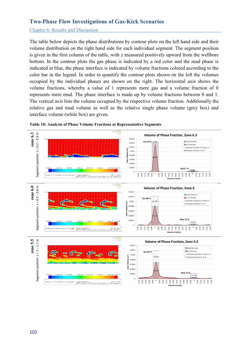
Two-Phase Flow Investigations of Gas-Kick Scenarios
Chapter 6: Results and Discussion
102
The table below depicts the phase distributions by contour plots on the left hand side and their
volume distribution on the right hand side for each individual segment. The segment position
is given in the first column of the table, with z measured positively upward from the wellbore
bottom. In the contour plots the gas phase is indicated by a red color and the mud phase is
indicated in blue, the phase interface is indicated by volume fractions colored according to the
color bar in the legend. In order to quantify the contour plots shown on the left the volumes
occupied by the individual phases are shown on the right. The horizontal axis shows the
volume fractions, whereby a value of 1 represents mere gas and a volume fraction of 0
represents mere mud. The phase interface is made up by volume fractions between 0 and 1.
The vertical axis lists the volume occupied by the respective volume fraction. Additionally the
relative gas and mud volume as well as the relative single phase volume (grey box) and
interface volume (white box) are given.
Table 10: Analysis of Phase Volume Fractions at Representative Segments
zon
e 5
.5
Segm
ent
po
siti
on
: z
= 1
– 1
.1 m
zon
e 6
.3
Segm
ent
po
siti
on
: z
= 0
.2 –
0.3
m
zon
e 6
.0
Segm
ent
po
siti
on
: z
= 0
.5 –
0.6
m

Two-Phase Flow Investigations of Gas-Kick Scenarios
Chapter 6: Results and Discussion
103
zon
e 5
.0
Segm
ent
po
siti
on
: x:
1.5
– 1
.6m
zon
e 4
.5
Segm
ent
po
siti
on
: z
= 2
– 2
.1 m
The gas is entering the annulus at z = 0.12 m thereby reducing the available cross sectional
area for the mud passage and forcing it to travel upwards as a thin film along the inner pipe.
The displaced mud accelerates from initially 5 m/s to a maximum speed of about 65 m/s, see
Figure 89. The axial mixture velocity profiles shown are located at a radius of 0.084 m and
0.1016 m from the wellbore axis. The location of the profiles was picked to ensure the
profiles are lying within either the gas or the mud phase. Thus the red line shows the fluid
velocity where the presence of gas and the blue line shows the velocity profile where the
presence of mud is predominant. The negative velocity peak of the red series represents the
occurrence of a recirculation swirl just above the gas-kick inlet. High frequency fluctuations
zon
e 4
.0
Segm
ent
po
siti
on
: z
= 2
.5 –
2.6
m
zon
e 3
.6
Segm
ent
po
siti
on
: z
= 2
.9 –
3 m

Two-Phase Flow Investigations of Gas-Kick Scenarios
Chapter 6: Results and Discussion
104
in the profile are due to phase changes at these positions, so for instance the fluctuations in the
mud velocity profile directly after the gas-kick inlet are caused by the wave geometry of the
mud film travelling up the drill pipe. Disturbances start forming at the phase interface. The
initially wavy structure deforms more and more, as a consequence of shear between the
phases. Wave heights are increasing and begin to break up at the crests into smaller fluid
ligaments. The direction of rotation of the fluid ligaments indicates the faster phase. Breakup
of the liquid film is emphasized near the wall where axial shear is largest. Fluid ligaments and
droplets near the core are less sheared and therefore larger in size. The width of the strong
breakup and phase mixing zone near the drill pipe increases with distance from the wellbore
bottom. The phase mixing zone induces turbulences and approaches further into the annular
gap until a chaotic regime is eventually reached.
Figure 89: Axial Velocity Profile, LFK_7211
To illustrate the sharpness of the phase interface, standard deviations of the single phase
volume fractions are computed. Therefore a volume fraction of 0.5 was chosen to distinguish
between mud and gas phase. The basis for this calculation is a mean of 1 for the gas phase and
a mean of 0 for the mud phase. Assuming the gas and mud phase fractions to be normally
distributed the interval ± of the mean would contain 68.27% of the values.
Figure 90: Volume Fraction Standard Deviation
Figure 91: Single Phase and Interface Volume
Figure 90 illustrates the standard deviations of the gas and mud phase volume fractions along
the wellbore. The standard deviations are computed for each 10 cm zone segment. Low values
near the gas-kick entry at the wellbore bottom indicate a sharp phase interface and clear phase
separation; whereas high values further upwards the annulus illustrate the phase breakup into
very small droplets and bubbles. The computational grid resolution of 0.5 mm is not able to
resolve these very small flow structures and hence the volume occupied by the phase interface
increases. It should be noted that effects like numerical diffusion may also start to play a role

Two-Phase Flow Investigations of Gas-Kick Scenarios
Chapter 6: Results and Discussion
105
in these “smeared phase conditions”. Figure 91 provides information on how much volume is
occupied by a distinct single phase, i.e. volume fractions of 1 or 0, and how much volume is
occupied by the phase interface.
Figure 92: Phase Interface Area
Figure 93: Phase Interface Area based on VOF
The interface surface area can be calculated based on a certain volume fraction that defines
the border between the phases. This approach is appropriate when the interface is very sharp.
However the more the phase interface gets smeared the more difficult it is to define a single
volume fraction as the divider between the phases. Figure 92 shows the effect of increasing
phase interface volume on computed surface area for three selected volume fractions. In flow
domains where the interface is distinct the computed surface area should be independent on
volume fraction. As the volume occupied by the phase interface increases the computed
surface areas differ more widely. It can be seen that the interface area computed based on a
volume fraction of 0.5 is remaining almost constant although further breakup is occurring.
Especially cells containing small fluid droplets, i.e. cells with a volume fraction of 0.8, will
cause an increase in computed surface area along the annulus. Cells that are predominantly
filled with mud are decreasing further up the annulus and contribute less to the computed
interface area. Figure 93 shows the computed phase interface area of the whole model domain
based on different volume fractions.
The calculated standard deviation of phase volume fractions can be used as a measure for the
sharpness of the phase interface. It provides a means to assess whether the flow is clearly
separated or if it becomes dispersed and grid resolution needs to be refined. It may also be
used to estimate the phase interface area in zones where the flow structures are not fully
resolved. Based on the standard deviation one selects the volume fraction bounds for the bulk
gas and mud phase. The volume between these bounds is assumed to contain many small
droplets or bubbles that could not be resolved with the current grid. Based on the current mesh
resolution fluid entities down to a size of 4 mm can be resolved. Droplets or bubbles with a
smaller diameter can contribute substantially to the available interface area for mass transfer
between the phases. The phase interface area computed based on a volume fraction of 0.5
would then be just a rough estimate. The surface introduced by small droplets need to be
added to obtain the overall available interface area. A measure for the volume occupied by
these droplets is given by the mud volume fraction contained in the phase interface volume.
However assumptions would need to be made regarding the droplet size and size distribution.
Figure 94 shows an example on how the phase interface area would differ when taking into
account the interface area due to droplets and bubbles that are currently not being resolved.

Two-Phase Flow Investigations of Gas-Kick Scenarios
Chapter 6: Results and Discussion
106
The graph illustrates the stacked interface area per channel segment. The smallest portion is
due to the interface area calculated based on a volume fraction of 0.5, the largest portion is
made up by gas bubbles (d~0.1 mm) and second largest portion is made up by mud droplets
(d~1 mm). The calculation is based on a critical Weber number, predicting a stable bubble or
droplet size based on equality of kinetic energy and surface energy. For the calculation the
local phase velocity differences need to be evaluated. This analysis is very cumbersome and
based on too many assumptions and therefore not further pursued. It is just illustrated here to
give an impression on how big probably the influence of unresolved fluid structures could be
and the limitation of interface area computation. The definition of critical droplet or bubble
diameter is given below.
𝑊𝑒∗ =𝐸𝑘𝑖𝑛
𝐸𝑠𝑢𝑟𝑓 , 𝐸𝑘𝑖𝑛 =
𝜋𝜌𝑑2𝑈𝑟2
12, 𝐸𝑠𝑢𝑟𝑓 = 𝜋𝑑2𝜎
𝑑 =12𝜎
𝜌𝑈𝑟2
Ur relative velocity ρ fluid density d stable droplet/bubble diameter
surface tension
Figure 94: Interface Area per Segment
The following sequence of images (Fehler! Verweisquelle konnte nicht gefunden werden.
to Figure 97) shows a snapshot of the transient flow simulation and the computed gas
dissolution. Naturally there are local and timewise fluctuations in dissolved gas as a
consequence of the mixing process. To ease the comparison of simulation results in the next
section, values will be averaged over the annular cross section after the flow has fully
developed.

Two-Phase Flow Investigations of Gas-Kick Scenarios
Chapter 6: Results and Discussion
107
Figure 95: Detected Phase Interface
Figure 96: Gas Solubility [mol/m³]
Figure 97: Dissolved Gas [mol/m³]
Next the selected lateral fracture kick simulation cases listed in Table 8 will be compared
focusing on gas dissolution and associated parameters. Superficial mud velocity is the same
for all cases since the mass flow boundary is equal. To determine the superficial gas velocity
the mass flow rate and density at the gas inlet was measured. Based on superficial fluid
velocities the expected flow regime of the simulation cases is illustrated in the flow pattern
map for concentric vertical annuli provided by Caetano (1992), see Figure 98. According to
the flow pattern map, simulation case LFK_6 is located right at the border between dispersed
bubble flow and churn flow, the simulation cases LFK_0 and LFK_1 are both situated in the
churn flow regime, and simulation case LFK_7211 is marked at the edge to annular flow.
Looking at the snapshots of phase distribution provide in Figure 99 to Figure 102 the
suggested classification appears quite realistic.
The differential pressure at kick onset is increased by a factor of ~10 between the simulation
cases LFK_6, LFK_0, LFK_1 and by a factor of ~4 between the simulation cases LFK_1 and
LFK_7211. The mean axial velocity along the annulus is shown in Figure 103. The computed
specific interface area shows a similar trend for LFK_0 and LFK_1. Both are in the churn
flow regime according to the flow pattern map. The clearly separated flow in the lower half of
the annular channel causes a minimum phase interface area and is then followed by a strong
interface area increase due to the evolving churn type flow. The smallest gas inflow in case
LFK_6 is dispersing directly after the inlet, providing the highest phase interface area in this
section, thereafter only slight breakup follows indicated by a moderate increase in specific
interface area. The specific interface area belonging to the gas-kick scenario with the highest
initial pressure difference, LFK_7211, shows an increase shortly after the separated flow at
the gas inlet and is then slowly growing due to the breakup of liquid droplets in the gas
stream. Since the gas will accelerate further on its way up the annulus due to expansion, the
droplets will continue to breakup. Therefore the specific interface area plot may be
extrapolated. The average gas volume fraction plot per simulation case depicted in Figure 104
indicates a correlation with flow regime.
direction of flow outer cylinder
inner cylinder

Two-Phase Flow Investigations of Gas-Kick Scenarios
Chapter 6: Results and Discussion
108
Basically the flow regimes for all simulation cases will change towards annular flow with
decreasing wellbore depth. The gas density decreases causing gas expansion shown by an
increase in gas volume fraction. The entering mass flow of gas at the wellbore bottom stays
the same or is even increasing due to a pressure drop in the wellbore. The decrease in gas
density causes superficial gas velocities to increase on the way up to the surface whereas
superficial mud velocities will stay the same as long as no mud is lost to the formation. As a
consequence the kick scenario for an entire wellbore can be illustrated by a line in the flow
pattern map, pointing from dispersed to annular flow. The starting point is defined by the
pressure differential at kick onset and the bottom-hole pressure affecting gas density. The
length of the segment is defined by the difference in bottom-hole and well head pressure. The
lower the well head pressure the longer is the range in the flow regime map. However if gas
dissolution occurs this line may be interrupted. For instance a kick scenario starts with a
bubbly flow regime, gas dissolves and a single phase flow section follows, with decreasing
solubility up the annulus gas comes out of solution, starting as dispersed flow but due to gas
phase expansion a churn flow period follows until annular flow is reached. For gas dissolution
the influence of flow regime on the interface area and on the mass transfer coefficient is
crucial.
Figure 107 and Figure 108 show plots of the average mass transfer coefficient based on the
two modeling approaches, i.e. Sherwood correlation based computation and the model of
Kataoka and Miyauchi (1969) taking into account turbulent energy dissipation. Differences
are mainly due to the entry effects, especially the high velocity simulation case LFK_7211
shows the highest mass transfer coefficient when taking into account turbulent energy
dissipation. Further up the annulus mass transfer coefficients remain rather stable and can be
grouped by flow regime, this is especially true for the Sherwood correlation based values. In
general there is a large difference of a factor of ~50 between the two approaches.
Consequently the same difference between the two models is found in the computed mass
transfer rate, shown in Figure 107 and Figure 108. The fluctuations in mass transfer rate are
due to the fluctuations in phase interface area.
Finally the concentration of dissolved gas along the annular model section is given in Figure
111 and Figure 112. Due to the continuous supply of fresh mud, the concentration of
dissolved gas is lowest near the wellbore bottom and increases with elevation. The difference
between the Sherwood correlation based computation and the turbulence based model by
Kataoka is enormous. Extrapolating the dissolved gas profiles further up the annulus, Figure
113 and Figure 114, show the distance needed to reach full gas saturation of the mud.

Two-Phase Flow Investigations of Gas-Kick Scenarios
Chapter 6: Results and Discussion
109
Figure 98: Flow Pattern Map for Concentric Annuli, Caetano (1992)
Figure 99: LFK_6
Figure 100: LFK_0
Figure 101: LFK_1
Figure 102: LFK_7211

Two-Phase Flow Investigations of Gas-Kick Scenarios
Chapter 6: Results and Discussion
110
Figure 103: Average Axial Mixture Velocity
Figure 104: Average Gas Volume Fraction
Figure 105: Specific Interface Area
Figure 106: Gas Solubility
Figure 107: Mass Transfer Coefficient (Sherwood
Correlation)
Figure 108: Mass Transfer Coefficient (Kataoka
Model)
Figure 109: Mass Transfer Rate (Sherwood
Correlation)
Figure 110: Mass Transfer Rate (Kataoka Model)

Two-Phase Flow Investigations of Gas-Kick Scenarios
Chapter 6: Results and Discussion
111
Figure 111: Dissolved Gas Concentration
(Sherwood Correlation)
Figure 112: Dissolved Gas Concentration (Kataoka
Model)
Figure 113: Distance to Reach Full Mud Saturation
(Sherwood Correlation)
Figure 114: Distance to Reach Full Mud
Saturation (Kataoka Model)
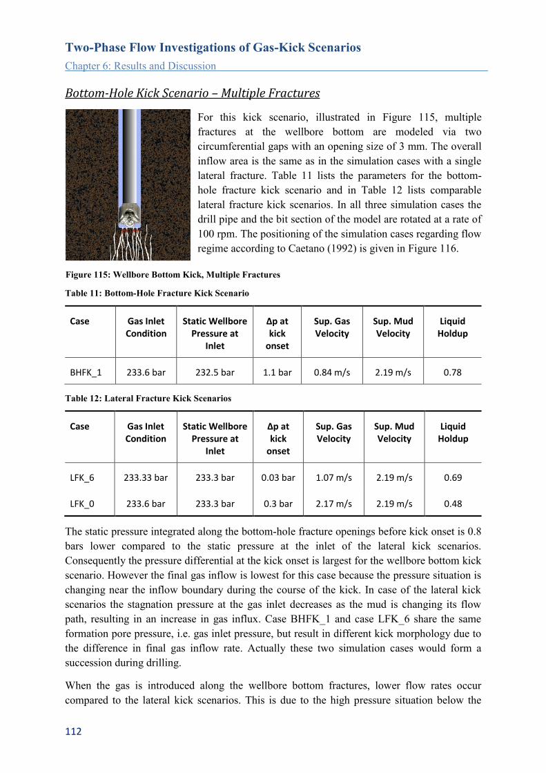
Two-Phase Flow Investigations of Gas-Kick Scenarios
Chapter 6: Results and Discussion
112
Bottom-Hole Kick Scenario – Multiple Fractures
For this kick scenario, illustrated in Figure 115, multiple fractures at the wellbore bottom are modeled via two
circumferential gaps with an opening size of 3 mm. The overall
inflow area is the same as in the simulation cases with a single
lateral fracture. Table 11 lists the parameters for the bottom-
hole fracture kick scenario and in Table 12 lists comparable
lateral fracture kick scenarios. In all three simulation cases the
drill pipe and the bit section of the model are rotated at a rate of
100 rpm. The positioning of the simulation cases regarding flow
regime according to Caetano (1992) is given in Figure 116.
Table 11: Bottom-Hole Fracture Kick Scenario
Case Gas Inlet Condition
Static Wellbore Pressure at
Inlet
∆p at kick
onset
Sup. Gas Velocity
Sup. Mud Velocity
Liquid Holdup
BHFK_1 233.6 bar 232.5 bar 1.1 bar 0.84 m/s 2.19 m/s 0.78
Table 12: Lateral Fracture Kick Scenarios
Case Gas Inlet Condition
Static Wellbore Pressure at
Inlet
∆p at kick
onset
Sup. Gas Velocity
Sup. Mud Velocity
Liquid Holdup
LFK_6 233.33 bar 233.3 bar 0.03 bar 1.07 m/s 2.19 m/s 0.69
LFK_0 233.6 bar 233.3 bar 0.3 bar 2.17 m/s 2.19 m/s 0.48
The static pressure integrated along the bottom-hole fracture openings before kick onset is 0.8
bars lower compared to the static pressure at the inlet of the lateral kick scenarios.
Consequently the pressure differential at the kick onset is largest for the wellbore bottom kick
scenario. However the final gas inflow is lowest for this case because the pressure situation is
changing near the inflow boundary during the course of the kick. In case of the lateral kick
scenarios the stagnation pressure at the gas inlet decreases as the mud is changing its flow
path, resulting in an increase in gas influx. Case BHFK_1 and case LFK_6 share the same
formation pore pressure, i.e. gas inlet pressure, but result in different kick morphology due to
the difference in final gas inflow rate. Actually these two simulation cases would form a
succession during drilling.
When the gas is introduced along the wellbore bottom fractures, lower flow rates occur
compared to the lateral kick scenarios. This is due to the high pressure situation below the
Figure 115: Wellbore Bottom Kick, Multiple Fractures

Two-Phase Flow Investigations of Gas-Kick Scenarios
Chapter 6: Results and Discussion
113
drill-bit. The gas entering the wellbore trough the fractures gets sheared off by the rotating
motion of the fluid representing the drill bit. Due to this process the kick gas is dispersed into
bubbles and strong mixing of the phases occurs. These bubbles move upward through the
drill-bit zone, where the injected drilling fluid is forming two large vortices representing the
drill bit. While the gas bubbles pass through the vortices, some of them get caught by the
swirling fluid, collide, coalesce and form larger bubbles caught in the vortices center.
The instantaneous phase distribution along the annulus after the flow has stabilized is shown
in Figure 117 to Figure 120. In the lower model section rotating flow structures can be found
as a consequence of the inlet configuration. The middle section shows axially sheared fluid
ligaments, an indication for differences in axial gas and mud velocity. Eventually gas bubble
shape becomes more distinct in the upper section of the model, which is basically a matter of
low differential fluid velocity in the core of the channel and stronger shear near the walls
causes smearing of the phases.
Figure 116: Flow Pattern Map for Concentric Annuli, Caetano (1992)

Two-Phase Flow Investigations of Gas-Kick Scenarios
Chapter 6: Results and Discussion
114
Figure 117: BHFK_1,
Phase Distribution
Figure 118:
Upper Section
Figure 119:
Middle Section
Figure 120:
Lower Section
A time history of gas contact at the inner pipe is illustrated in Figure 121. The inner pipe is
split into 7 sections starting at the upper model end. Each series represents the average gas
contact versus time of one segment. Impact of gas on the inner pipe is pronounced at the
beginning of the channel and then gradually vanishes when travelling up the annulus. Due to
| l
ow
er
sect
ion
|
mid
dle
se
ctio
n
|
up
pe
r se
ctio
n
|

Two-Phase Flow Investigations of Gas-Kick Scenarios
Chapter 6: Results and Discussion
115
the vortices at the annulus the gas is first pushed to the inner pipe and then eventually
accumulating in the channel core.
Figure 121: Gas Contact at Inner Pipe, BHFK_1
Monitoring the cross sectional distribution of the gas after the flow has become steady, it was
found that the gas mud ratio near the channel walls remains rather stable while the largest
fluctuations in volume fraction are found in the channel core; see Figure 123 and Figure 124.
There are three peaks according to the travel paths of the gas fraction. The large gas bubbles
denote the largest peak located the outer third of the annular gap, and the small gas bubbles
form two pathways close to the walls. The asymmetry of the cross-sectional profiles is due to
the annular conduit geometry; in a pipe the profiles would be symmetrical. Naturally the
fluctuations in gas volume fraction occur since the gas is not flowing as a continuous stream
of a bulk fluid. The three peaks showing up in the cross sectional gas volume distribution
indicate that the flow regime is not a mere bubble flow but instead, especially due to the
larger bubbles, close to a transition to slug flow. Experimental investigations of vertically
upward flow in pipes conducted by Serizawa and Kataoka (1987) and illustrated in Figure 122
show similar profiles of void fraction distribution. They observed the transition from bubble
to slug flow being accompanied by a change in void fraction profile from wall peaking to core
peaking.
Figure 122: Void Fraction Distribution of Vertically Upward Flow in Pipes, Serizawa and Kataoka (1987)
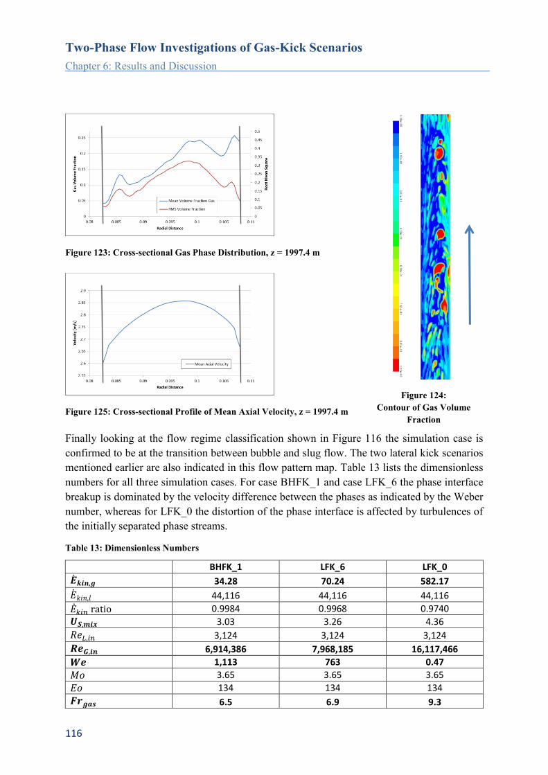
Two-Phase Flow Investigations of Gas-Kick Scenarios
Chapter 6: Results and Discussion
116
Figure 123: Cross-sectional Gas Phase Distribution, z = 1997.4 m
Figure 124:
Contour of Gas Volume
Fraction
Figure 125: Cross-sectional Profile of Mean Axial Velocity, z = 1997.4 m
Finally looking at the flow regime classification shown in Figure 116 the simulation case is
confirmed to be at the transition between bubble and slug flow. The two lateral kick scenarios
mentioned earlier are also indicated in this flow pattern map. Table 13 lists the dimensionless
numbers for all three simulation cases. For case BHFK_1 and case LFK_6 the phase interface
breakup is dominated by the velocity difference between the phases as indicated by the Weber
number, whereas for LFK_0 the distortion of the phase interface is affected by turbulences of
the initially separated phase streams.
Table 13: Dimensionless Numbers
BHFK_1 LFK_6 LFK_0
𝒌𝒊𝒏,𝒈 34.28 70.24 582.17
𝑘𝑖𝑛,𝑙 44,116 44,116 44,116
𝑘𝑖𝑛 ratio 0.9984 0.9968 0.9740
𝑼𝑺,𝒎𝒊𝒙 3.03 3.26 4.36
𝑅𝑒𝐿,𝑖𝑛 3,124 3,124 3,124
𝑹𝒆𝑮,𝒊𝒏 6,914,386 7,968,185 16,117,466
𝑾𝒆 1,113 763 0.47
𝑀𝑜 3.65 3.65 3.65
𝐸𝑜 134 134 134
𝑭𝒓𝒈𝒂𝒔 6.5 6.9 9.3

Two-Phase Flow Investigations of Gas-Kick Scenarios
Chapter 6: Results and Discussion
117
Ri 5,788 8,199 13,431,012
In context with flow patterns it is interesting to have a look at the frequencies of the occurring
fluctuations in mud flow rate. For a sample analysis the mud flow rates at the model outlet
were monitored for simulation case LFK_0 and BHFK_1, shown in Figure 126 and Figure
127 respectively. The mud rate log of LFK_0 clearly shows an initial plug displacement of the
mud by the gas. Once the gas has reached the outlet of the model domain the mud flow rate
starts to become volatile as a consequence of the 2-phase churn flow situation evolving. The
time averaged mud flow rate approaches the pump rate indicating steady state. The shape of
the mud flow rate history of case BHFK_1 sows quite a different behavior. In this case the
low gas influx is not strong enough to cause a plug type displacement of the mud; instead the
entering gas bubbles initiate a pulsatile mud flow.
The monitored flow rate at the upper exit of the model domain is equivalent to the mud return
being observed at the well head, as long as no gas has left the domain. While gas travels up
the annulus, the returning mud flow rate will be additionally increased due to expansion of the
gas. Flow rate indicators are able to measure small increases in flow rate and can trigger
warnings regarding kicks before pit level gains can be detected. Therefore, an observed
increase in flow rate is usually one of the first indicators of a kick.
Figure 126: Mass Flow Rates, LFK_0
Figure 127: Mass Flow Rates, BHFK_1
Figure 128 and Figure 129 show the Fast Fourier Transform (FFT) of the mud flow rate for
selected time periods, where the mud fluctuations and respective flow patterns appear to be
more or less constant. For the lateral gas-kick three distinctive peaks where found in the
spectral density plot i.e. at 13, 23 and 31 Hz. The results were visually compared with phase
contour plots at the selected time period. All three frequencies correspond to a wispy annular
flow regime, with a wavy mud film travelling up along the drill pipe and the outer cylinder
being in contact with dry gas. Each frequency is indicating a characteristic flow entity size,
for instance a fluid ligament or wave, as can be seen in the flow pattern plot in Figure
130Figure 130. In case of the gas-kick entering at wellbore bottom two time periods were
analyzed. First a time period from 0.5 to 1 second; during this time no gas has reached the
model outlet, but we can observe a pulsatile mud flow caused by the entering gas bubbles.
During this time frame two 2 high frequency peaks at 113 and 157 Hz are observed. The
explanation for these two peaks is that there must be at least two characteristic bubble or slug

Two-Phase Flow Investigations of Gas-Kick Scenarios
Chapter 6: Results and Discussion
118
sizes appearing repeatedly in a short time interval at the entry of the annulus. If bubbles would
be generated arbitrarily with a uniform size distribution, such prominent peaks could not be
observed. Instead the outcome of the FFT analysis would look like a random signal. At the
second time frame (1.3 to 2.2 s) gas has reached the outlet and a stable flow pattern has
established. A very distinctive peak at a frequency 132 Hz can be seen. Again this tells us that
there must be a periodic appearance of similar sized flow entities. The phase contour plot in
Figure 131 illustrates the origin of the two frequency peaks. The large gas pockets generated
at the entry of the annulus with a length of approximately 1.8 cm and a separation distance of
4 cm, travelling at a velocity of 6 m/s are responsible for the frequency peak at 157 Hz. The
longer fluid ligaments besides the gas slugs are rising at a lower velocity and show a
frequency of roughly 113 Hz. Finally the flow pattern in Figure 157Figure 132 shows the
repeating occurrence of larger gas bubbles in the core flow at the model outlet with a
frequency of 132 Hz.
Regarding the selected simulation cases this type of analysis provides us with the
understanding that larger flow structures will result in slower fluctuations whereas smaller
flow structures like bubbles will result in higher fluctuation frequencies. Additionally the size
of the flow structures is making a clear footprint in the frequency domain. It should also be
noted that especially for gas-kicks with larger flow rates, the increasing amount of gas in the
annulus will tend to dampen flow and pressure fluctuations resulting in smoother time
histories and less pronounced peaks in the frequency domain. Summing up this analysis
shows that the time history of mud pulsations contains valuable information in terms of 2-
phase flow morphology.
Figure 128: FFT of Mud Flow Rate, LFK_0
Figure 129: FFT of Mud Flow Rate, BHFK_1

Two-Phase Flow Investigations of Gas-Kick Scenarios
Chapter 6: Results and Discussion
119
Figure 130:
Flow Pattern at Model Outlet,
LFK_0, t = 2.45 s
Figure 131: Flow Pattern at
Annular Entry, BHFK_1, t =
0.63 s
Figure 132: Flow Pattern at
Model Outlet, BHFK_1, t =
2.24 s
Figure 133 illustrates the transient change of flow patterns for simulation case BHFK_1 and
LFK_0. Calculation of superficial velocities is based on the flow rates and gas density
monitored at the model outlet. Both cases begin with a dispersed bubble flow when the first
gas enters the wellbore. The higher superficial mud velocity of case LFK_0 is due to the mud
displacement caused by the gas, seen as pit gain at the surface. Basically case LFK_0 shows a
broader range of values compared to case BHFK_1.
Figure 133: Flow Pattern Map for Concentric Annuli, Caetano (1992)
Finally the three simulation cases listed in Table 11 and Table 12 are compared with respect
to gas dissolution and its major parameters. The details are illustrated in Figure 134 to Figure
145. Simulation cases LFK_6 and BHFK_1 both show dispersed flow characteristics. Both
cases show similar gas flow rates as reflected by the average axial mixture velocities in Figure
134. Average gas volume fraction is largest for simulation case LFK_0. The highest gas
volume fraction is found next to the gas inlet, it is then decreasing along a separated flow

Two-Phase Flow Investigations of Gas-Kick Scenarios
Chapter 6: Results and Discussion
120
section until the fluctuations indicate the onset of the churn flow regime. The volume fraction
series of case LFK_0 similarly starts with a high gas volume fraction near the inlet; this
appears to be characteristic for this inlet location. The smooth profile of simulation case
BHFK_1 is due to the finely dispersed gas volume fraction. Specific interface area illustrated
in Figure 136 shows lowest values for the separated flow section of case LFK_0. Further up
the annulus the phase interface is strongly increasing due to the enhanced breakup in the
churn flow regime. Specific interface area values of the two dispersed flow cases range within
the same bounds. The computed mass transfer coefficients show a similar trend for both
approaches. Mass transfer coefficients of case LFK_6 and BHFK_1 only differ near the
lateral gas inlet. Mass transfer coefficients of case LFK_0 clearly show the influence of the
velocity difference between gas and mud. The highest velocity difference occurs at the lateral
gas inlet. Gas and mud velocity then gradually aligns, which is accompanied by a decrease in
mass transfer coefficient reaching a minimum were gas and mud are flowing at equal speed.
After that buoyancy is the mere factor causing relative fluid velocities resulting in random
fluctuations of the mass transfer coefficient. In case of the Sherwood-based approach the
shape of the computed mass transfer rate profiles reflects the profile of the specific phase inter
face area. The higher mass transfer coefficients of the Kataoka model level out the lower
specific interface area at the beginning of the annulus in case of LFK_0. The difference
between the mass transfer computation approaches for simulation case BHFK_1 accounts for
a factor of ~ 10. The two dispersed flow simulation cases show the highest concentration in
dissolved gas. Finally extrapolating the dissolved gas profiles further up the annulus shows
the distance needed to reach full gas saturation of the mud in Figure 144 and Figure 145.

Two-Phase Flow Investigations of Gas-Kick Scenarios
Chapter 6: Results and Discussion
121
Figure 134: Average Axial Mixture Velocity
Figure 135: Average Gas Volume Fraction
Figure 136: Specific Interface Area
Figure 137: Gas Solubility
Figure 138: Mass Transfer Coefficient (Sherwood
Correlation)
Figure 139: Mass Transfer Coefficient (Kataoka
Model)
Figure 140: Mass Transfer Rate (Sherwood
Correlation)
Figure 141: Mass Transfer Rate (Kataoka Model)
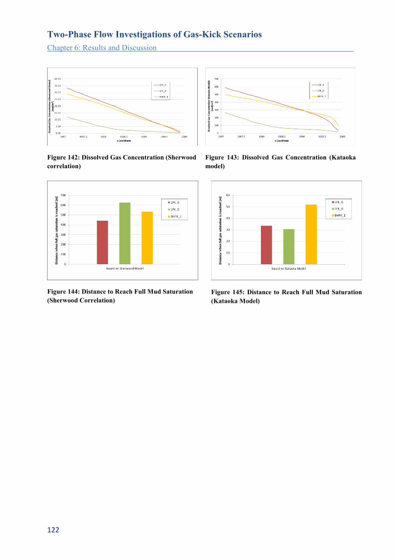
Two-Phase Flow Investigations of Gas-Kick Scenarios
Chapter 6: Results and Discussion
122
Figure 142: Dissolved Gas Concentration (Sherwood
correlation)
Figure 143: Dissolved Gas Concentration (Kataoka
model)
Figure 144: Distance to Reach Full Mud Saturation
(Sherwood Correlation)
Figure 145: Distance to Reach Full Mud Saturation
(Kataoka Model)

Two-Phase Flow Investigations of Gas-Kick Scenarios
Chapter 6: Results and Discussion
123
Loss of Mud Circulation
When drilling into highly fractured formations, formations with high permeability or
cavernous formations loss of drilling mud circulation can occur. Drilling mud will then flow
into the surrounding formation causing no or reduced mud flow to the surface. The loss of
fluid reduces the hydrostatic pressure in the wellbore and when it becomes lower than the
formation pressure gas enters the wellbore and causes a kick. To investigate the possibility of
lost circulation during a gas-kick event several model scenarios were simulated. These
scenarios cover both constant pressure and constant mass flow inlet boundary conditions at
dedicated kick locations. The pressure inlet boundary it is not restricted to the gas phase but
also allows the passage of mud. The modeled scenarios range from a cavernous gas inlet area
located either directly below the drilling bit or laterally next to the wellbore bottom.
Lateral Kick Scenario – Cavernous Opening
This kick scenario represents a gas inflow from a cavernous
opening located laterally of the drill bit. The large inlet area
provokes a massive inflow of formation gas. Two simulations
with different gas inlet conditions are compared. Table 14 lists
the main differences between the simulation cases. In both
setups the inner pipe, drill bit and annular channel are rotated at
a rate of 100 rpm. In case LCK_1 a pressure boundary
condition of 233.3 bars is applied at the gas inlet. This
corresponds to a pressure differential of 1.8 bars at kick onset.
Case LCK_2 is setup with a constant mass flow inlet of 3 kg/s
for the kick gas. The mass flow inlet condition refuses mud to
leave the wellbore. Consequently no loss of circulation can
occur even if the initial pressure situation would dictate it.
Table 14: Simulation Cases: Lateral Cavern Kick
Case Gas Inlet Condition
Static Wellbore Pressure at Inlet
Sup. Gas Velocity
Sup. Mud Velocity
Liquid Holdup
LCK_1 233.3 bar 231.5 bar 10.04 m/s 2.19 m/s 0
LCK_2 3 kg/s 1.43 m/s 2.19 m/s 0.56
The final (steady-state) phase distribution for both simulation cases is shown in Figure 147
and Figure 148 respectively. The peculiar shape of the phase interface near the wellbore
bottom is due to entrainment of the mud stream.
Figure 146: Lateral Kick
Scenario, Cavern

Two-Phase Flow Investigations of Gas-Kick Scenarios
Chapter 6: Results and Discussion
124
Figure 147: LCK_1
Figure 148: LCK_2
In LCK_1 all mud is lost to the formation and the gas-kick is fully occupying the annular
channel resulting in high gas superficial velocity of ~ 10 m/s. The mass flow rate of the gas
stabilizes at a value of 20.78 kg/s. The only resistance left for the gas on its way up the
annulus is the remaining mud column, until this scenario results in a blow-out.
In case of the mass flow boundary condition applied in LCK_2, the mud is forced to flow up
the annulus at its inflow rate since there is no alternative passage for the mud to escape into
the formation. As a consequence mud and gas is flowing concurrently upwards, clearly
separated by a smooth interface area. Eventually the mud is occupying 56 % of the annular
volume. The evolution of total gas volume fraction in the annular channel of this simulation
case is shown in Figure 149.

Two-Phase Flow Investigations of Gas-Kick Scenarios
Chapter 6: Results and Discussion
125
Figure 149: Total Gas Volume Fraction in Annulus, LCK_2
In LCK_2 gas entering the wellbore is changing the flow path for the mud. The space
occupied by the gas in the annulus reduces the available passage space for the drilling mud
and increases flow resistance. In the model the mud inflow is modeled by a constant mass
flow boundary, in reality a higher pump pressure would be needed to keep the circulation rate
at the same level. In general the selection of a constant mass flow boundary for the gas inlet,
prohibiting the loss of mud, appears to better match a kick situation where gas is escaping
from porous media instead of a cavern.
Regarding the simulation case LCK_1, a transient snapshot of the phase distribution at t=0.55
seconds after kick onset is shown in Figure 150. The mud phase shown in black is forming a
thin film on the wellbore bottom that is flowing radially outward into the formation. The gas
is pushing the remaining mud column in the annulus upwards. Some liquid is initially
attached at the outer cylinder and a few liquid ligaments are trapped in the gas core, but the
flow is basically separated.
Figure 150: LCK_1, t = 0.55 s

Two-Phase Flow Investigations of Gas-Kick Scenarios
Chapter 6: Results and Discussion
126
The dimensionless numbers characterizing the simulation cases are listed in Table 15. Since
the fluid properties and channel geometry are the same for both simulation cases, Morton and
Eötvös number are basically the same. There are only small differences in gas density due to
differences in pressure, but this is negligible. The dominant factor is the difference in gas
inflow velocity, expressed by the kinetic energy of the gas stream, high gas Reynolds number
and mixture velocity. A high Weber number represents the dominance of inertia forces
compared to surface tension force. It is a measure for phase interface distortion and is
proportional to the square of the phase slip velocity. The Weber number calculated for the
annulus is about 5 times higher looking at the transient snapshot of LCK_1 compared with the
smooth annular flow of LCK_2. The gas Froude number expresses the ratio of inertia to
buoyancy force. When the flow has reached steady state in the model, the gas Froude number
of the two simulation cases differs by a factor of ~3. However it is interesting to see that the
gas Froude numbers are quite similar when comparing the transient snapshot of LCK_1 with
the fully developed flow of LCK_2. This is because the gas inflow velocity is still increasing
as a result of the pressure inlet condition. Consequently the kinetic energy brought into the
system by the gas is still low. The superficial gas velocity at this stage amounts only 0.6 m/s,
naturally the phase slip is largest resulting in the breakup of the phase interface.
Table 15: Dimensionless Numbers, Lateral Cavern Kick
LCK_1, t = 0.55 s LCK_1 LCK_2
𝒌𝒊𝒏,𝒈 0.01 52.56 0.15
𝑘𝑖𝑛,𝑙 44,116 44,116 44,116
𝑘𝑖𝑛 ratio 1.00 0.9976 1.0000
𝑼𝑺,𝒎𝒊𝒙 2.81 12.23 3.62
𝑅𝑒𝐿,𝑖𝑛 3,124 3,124 3,124
𝑹𝒆𝑮,𝒊𝒏 4,599,816 75,263,131 10,865,707
𝑾𝒆 1,508 - 351
𝑀𝑜 3.65 3.65 3.64
𝐸𝑜 133 133 133
𝑭𝒓𝒈𝒂𝒔 6.0 26.0 7.7
Ri 4,145 168 17,782
The positioning of the simulation cases regarding flow regime according to Caetano (1992) is
given in Figure 151. According to this classification the simulation cases are located near the
lower and upper end of the churn flow regime. Despite the blow out scenario of simulation
case LCK_1, case LCK_2 does not confirm the churn flow prediction but instead shows
annular flow morphology. The reason for this deviation in flow morphology arises from the
applied rotation rate to drill pipe, drill bit zone, and annular channel. As discussed in Chapter
5: Influence of Rotation, a rotation rate of 100 rpm applied only to the inner cylinder will not
initiate any flow instabilities. This is also confirmed by the lateral gas kick scenarios, which
are well represented by the flow regime map of Caetano although the drill pipe is rotating. In
simulation case LCK_2 the rotation is not only applied to the inner cylinder and drill bit
section, but also to the annular fluid zone which results in a stronger influence on the flow
field. The fluid rotation causes an initial smoothing of the gas-liquid phase interface; any

Two-Phase Flow Investigations of Gas-Kick Scenarios
Chapter 6: Results and Discussion
127
radial discontinuity gets averaged in circumferential direction, as one can observe when
stirring in a coffee cup. The lateral gas inlet forces the mud stream to initially travel next to
the inner cylinder, however centrifugal forces will begin pushing the heavier fluid radially
outwards. To illustrate how the flow regime will be affected thereby, a longer model section
needs to be modeled. Nevertheless the wellbore section were rotation plays a dominant role
on flow morphology is limited to the near drill bit zone. Further up the annulus, were no
rotation is applied the centrifugal momentum will quickly vanish and be overruled by
buoyancy.
Figure 151: Flow Pattern Map for Concentric Annuli, Caetano (1992)

Two-Phase Flow Investigations of Gas-Kick Scenarios
Chapter 6: Results and Discussion
128
Bottom-Hole Kick Scenarios
For this setup it is assumed that the kick occurs at the bottom of the well while drilling. Two
possible configurations are sketched in Figure 152 and Figure 153. On the left the wellbore
approaches a large cavernous opening and on the right the bottom-hole area is assumed a
homogeneous porous layer.
Figure 152: Wellbore Bottom Kick Scenario,
Large Opening = Cavern
Figure 153: Wellbore Bottom Kick Scenario,
Porous Media Boundary
Table 16: Simulation Cases: Bottom-Hole Cavern Kick
Case Gas Inlet Condition
Rotation Sup. Gas Velocity
Sup. Mud Velocity
Liquid Holdup
BHPK_2 3 kg/s 100 rpm, channel 1.45 m/s 2.19 m/s 0.74
BHPK_4 3 kg/s 0 1.45 m/s 2.19 m/s 0.67
BHCK_32 234 bar 100 rpm, only bit 26 m/s 2.19 m/s 0
Three simulation cases are discussed; the main simulation parameters are listed in Table 16.
Case BHPK_2 and BHPK_4 apply a constant mass flow boundary for the kick gas and
BHCK_32 applies a pressure inlet condition. Again the pressure inlet condition realistically
reproduces any loss of circulation that may occur when drilling overbalanced into a cavern,
whereas the mass flow inlet condition prohibits any mud loss. Actually the latter can be
compared with a different geometric configuration, i.e. an adjacent porous media which is
permeable to the gas phase but impermeable to the mud phase, see Figure 153. This

Two-Phase Flow Investigations of Gas-Kick Scenarios
Chapter 6: Results and Discussion
129
assumption of impermeability for the mud is reasonable since the permeability for the gas is
way higher due to the high ratio in viscosity of the two fluids.
The positioning of the simulation cases with respect to flow regime classification according to
Caetano (1992) is given in Figure 154. The two simulation cases representing the porous
media boundary configuration share the same position in the churn flow regime of the map.
The position is defined by the identical gas superficial velocity, thus one would expect
identical flow morphology. However when looking at the phase distribution illustrated in
Figure 155 and Figure 157 a strong deviation in flow regimes can be seen.
Figure 154: Flow Pattern Map for Concentric Annuli, Caetano (1992)
The only difference between simulation case BHPK_2 and BHPK_4 is in terms of applied
rotation. For the former case a rotation rate of 100 rpm is applied to the whole fluid domain
and inner cylinder, and for the latter simulation case no rotation is active. The flow regime
map of Caetano is based on experiments without fluid rotation. Similarly to the lateral cavern
kick simulation studies discussed earlier a smoothing of the phase interface can be observed
due to fluid zone rotation.

Two-Phase Flow Investigations of Gas-Kick Scenarios
Chapter 6: Results and Discussion
130
Figure 155: BHPK_2
Figure 156: BHPK_4
Figure 157: BHCK_32
As can be seen from Table 17 the dimensionless numbers of both simulation cases are
identical although the phase distribution shown in Figure 155 and Figure 156 differs
considerably. This is due since none of the listed dimensionless numbers covers the effect of
rotation, which in this particular case turned out to be quite strong with respect to phase
interface distortion. A dimensionless number suitable to characterize the influence of rotation
is the Rossby number, described in Chapter 5: Influence of Rotation. The rotation applied to
the fluid zone appears to have a strong separating effect on the phases, especially close to the
wellbore bottom. The applied radial acceleration to the fluid due to pipe rotation is small and
it takes some time until this will push the mud towards the outer cylinder, especially when the
movement is overlapped by high axial velocities. Therefore the interface smoothening effect
due to the tangential velocity component is larger than the mixing effect due to the radial

Two-Phase Flow Investigations of Gas-Kick Scenarios
Chapter 6: Results and Discussion
131
velocity component. This can be seen in Figure 155, the heavier mud phase stays close to the
inner cylinder and the phase interface is very smooth. The evolving flow morphology
corresponds to annular flow as known from flow in pipes. The strong cross-sectional mixing
seen in Figure 156 is a result of fluid motion without any rotation applied. Figure 158 and
Figure 160 show histograms of axial and radial mixture velocities in the annular channel. The
simulation case with no rotation applied, BHPK_4, shows the broadest distribution of radial
velocity. The radial component due to radial phase displacement is larger than the radial
velocity induced by rotation. The circumferential velocity component induced by rotation is
smoothing the phase interface. When looking at the axial shear of the fluid in the annular
channel, see Figure 159, the simulation case without rotation shows an almost symmetric
distribution of axial shear and the simulation case with rotation shows two distinct ranges of
shear values. The lower range of axial shear is occurring at the gas-mud interface, the peak
with the higher axial shear values belongs to the axial shear occurring within the bulk mud.
Within the bulk gas the axial velocity is almost uniform and axial shear is a minimum.
Figure 158: Histogram of Radial Mixture Velocity
Figure 159: Axial Shear in Annular Channel
Figure 160: Histogram of Axial Mixture Velocity
Figure 161: Wall Shear Stress at Inner Pipe
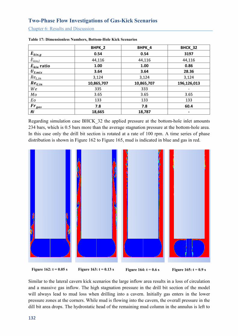
Two-Phase Flow Investigations of Gas-Kick Scenarios
Chapter 6: Results and Discussion
132
Table 17: Dimensionless Numbers, Bottom-Hole Kick Scenarios
BHPK_2 BHPK_4 BHCK_32
𝒌𝒊𝒏,𝒈 0.54 0.54 3197
𝑘𝑖𝑛,𝑙 44,116 44,116 44,116
𝒌𝒊𝒏 𝐫𝐚𝐭𝐢𝐨 1.00 1.00 0.86
𝑼𝑺,𝒎𝒊𝒙 3.64 3.64 28.36
𝑅𝑒𝐿,𝑖𝑛 3,124 3,124 3,124
𝑹𝒆𝑮,𝒊𝒏 10,865,707 10,865,707 196,126,013
𝑊𝑒 335 333 -
𝑀𝑜 3.65 3.65 3.65
𝐸𝑜 133 133 133
𝑭𝒓𝒈𝒂𝒔 7.8 7.8 60.4
Ri 18,665 18,787 -
Regarding simulation case BHCK_32 the applied pressure at the bottom-hole inlet amounts
234 bars, which is 0.5 bars more than the average stagnation pressure at the bottom-hole area.
In this case only the drill bit section is rotated at a rate of 100 rpm. A time series of phase
distribution is shown in Figure 162 to Figure 165, mud is indicated in blue and gas in red.
Figure 162: t = 0.05 s
Figure 163: t = 0.13 s
Figure 164: t = 0.6 s
Figure 165: t = 0.9 s
Similar to the lateral cavern kick scenarios the large inflow area results in a loss of circulation
and a massive gas inflow. The high stagnation pressure in the drill bit section of the model
will always lead to mud loss when drilling into a cavern. Initially gas enters in the lower
pressure zones at the corners. While mud is flowing into the cavern, the overall pressure in the
dill bit area drops. The hydrostatic head of the remaining mud column in the annulus is left to

Two-Phase Flow Investigations of Gas-Kick Scenarios
Chapter 6: Results and Discussion
133
counteract the gas inflow. As the pressure of the inflowing gas is higher and the well is not
closed, the mud is being pushed upwards until the whole channel of the model is filled with
gas. The increase in gas volume fraction in the modeled domain is shown in Figure 166. The
bend in the time series indicates the removal of the bulk mud. Remaining wall films are
removed after ~ 1.3 s when the whole channel is filled with gas.
Figure 166: BHCK_32, Gas Volume Fraction
Finally simulation case BHPK_2 and BHPK_4 are compared regarding gas dissolution and its
major parameters, see Figure 167 to Figure 178 for the details. Average axial mixture
velocities are nearly equal. Case BHPK_4 is showing a higher gas volume fraction and
naturally a much larger specific interface area along the annulus. However mass transfer
coefficients are very similar for both simulation cases. Both mass transfer coefficient
definitions show identical values for the two simulation cases near the gas entry and then
slowly deviate. Consequently the difference in computed mass transfer rate between BHPK_2
and BHPK_4 is induced by the difference in specific interface area. The difference between
the mass transfer computation approaches is again very big, it accounts for a factor of ~ 20,
but it is not as big as seen in the lateral fracture kick scenarios. The concentration of dissolved
gas along the annular model section is given in Figure 175 and Figure 176Figure 112. Due to
the increase in phase interface area case BHPK_4 deviates more and more from the
concentration profile of case BHPK_2. It is the small interfacial structures that are responsible
for the accumulation of dissolved gas in simulation case BHPK_4. Finally extrapolating the
dissolved gas profiles further up the annulus shows the distance needed to reach full gas
saturation of the mud.

Two-Phase Flow Investigations of Gas-Kick Scenarios
Chapter 6: Results and Discussion
134
Figure 167: Average Axial Mixture Velocity
Figure 168: Average Gas Volume Fraction
Figure 169: Specific Interface Area
Figure 170: Gas Solubility
Figure 171: Average Mass Transfer Coefficient
(Sherwood Correlation)
Figure 172: Average Mass Transfer Coefficient
(Kataoka Model)
Figure 173: Mass Transfer Rate (Sherwood
Correlation)
Figure 174: Mass Transfer Rate (Kataoka Model)
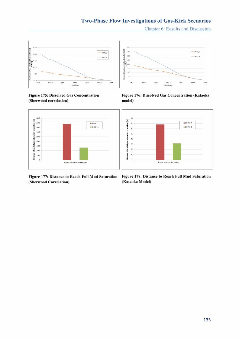
Two-Phase Flow Investigations of Gas-Kick Scenarios
Chapter 6: Results and Discussion
135
Figure 175: Dissolved Gas Concentration
(Sherwood correlation)
Figure 176: Dissolved Gas Concentration (Kataoka
model)
Figure 177: Distance to Reach Full Mud Saturation
(Sherwood Correlation)
Figure 178: Distance to Reach Full Mud Saturation
(Kataoka Model)

Two-Phase Flow Investigations of Gas-Kick Scenarios
Chapter 7: Conclusions
136
7. Conclusions
The significance of this thesis is to provide a better insight on the two-phase flow situation in
a well during a gas-kick and to provide means to assess the corrosive threat. For many
applications it is necessary to predict flow patterns as a basis for carrying out calculations on
two-phase flow. In the present study it was not the goal to make prior assumptions regarding
the evolving flow pattern but instead to gain more insight on two-phase interactions at a close-
up view. This thesis describes methodologies to characterize various flow aspects that are of
potential interest to corrosion engineers. One of the major difficulties in modeling the
corrosive risk to drill pipe during a gas-kick is the determination of the liquid and gas phase
distribution in the annulus. As significant chemical reactions are related to the size of the
phase interface area, a high resolution CFD simulation focusing on the gas and mud phase
distribution is provided. Based on the analysis of these simulation studies, a coarser full scale
model of the wellbore including chemical modeling can be established. Basically the kick
modeling had to be done without focusing on the validation aspect as such, since no suitable
experimental data was available.
Focus of the shown investigations was put on the near drill bit section. This inflow area shows
certain characteristics that are dominated by the inflow conditions of the gas as well as by the
configuration of the mud stream entering the annulus. After a certain distance, two-phase flow
has fully developed and the influence of the gas and fluid inlet configuration is no more
dominant. This entrance length accounts approximately 30 times the annular clearance. Stable
flow conditions when dealing with time averages have then developed and two-phase flow
correlations based on flow pattern maps are becoming valid. The flow pattern map provided
by Caetanto (1992) appears to cover well the investigated flow scenarios.
In vertical wellbores the flow pattern will gradually change due to the expansion of the gas
caused by the decrease in pressure along the vertical axis. The expansion of gas causes a
change in superficial gas velocity along the annulus. Furthermore the sudden inflow of gas
into the wellbore represents a transient flow situation, where the steady flow field established
by the circulation of the drilling fluid gets interrupted. The magnitude of kick influx is
governed by the pressure difference between formation pore pressure and wellbore stagnation
pressure at the wellbore-formation interface. While the fluid pressure in the formation will
stay more or less constant during the kick, the pressure in the wellbore is subject to change.
Two-phase flow patterns mainly depend on the flow rates, geometry and fluid properties of
the phases. While the latter two remain more or less the same, it is the flow rates that are
continuously changing during a kick. Consequently the two-phase flow pattern will also be
subject of change until a new steady flow situation establishes.
As a consequence there is no single flow pattern for an entire wellbore, flow patterns are
changing with time and location. Basically the flow regimes will change towards annular flow
with decreasing wellbore depth. Based on superficial velocities a range of flow patterns can
be defined for a kick event, illustrated as a line in the flow pattern map when the mud rate is

Two-Phase Flow Investigations of Gas-Kick Scenarios
Chapter 7: Conclusions
137
kept constant and no mud is lost to the formation. The starting point is defined by the pressure
differential at kick onset and the static bottom-hole pressure affecting gas density. The length
of the segment is defined by the difference in bottom-hole and well head pressure. The lower
the well head pressure the longer is the range in the flow regime map. However if gas
dissolution occurs this line may be interrupted. For instance a kick scenario starts with a
bubbly flow regime, gas dissolves and a single phase flow section follows, with decreasing
solubility up the annulus gas comes out of solution, starting as dispersed flow but due to gas
phase expansion a churn flow period follows until annular flow is reached.
For gas dissolution the influence of flow regime reflected via phase interface area and mass
transfer coefficient is the crucial factor. The available phase interface area thus turns out to be
the most important parameter to provide a basis for the assessment of corrosive risk.
The gas phase itself has no impact on drill pipe corrosion. It is the water that must be present
for sulfide stress cracking to occur. Therefore the simulation model was extended with user
defined functions to compute mass transfer due to gas dissolution based on two different
modeling approaches. One approach is based on a traditional Sherwood correlation and the
other one is based on the model of Kataoka (1969) accounting for the effect of turbulence on
mass transfer. The computed values differ considerably. In the Kataoka model fluid motion
enhances mass transfer due to turbulence dissipation. In the Shewood approach fluid motion
is accounted via a change in fluid viscosity through the rheological model. Basically
convection is governing the transport of species to the phase interface, where species are
crossing the interface due to diffusion. So increasing convection can enhance the mass
transfer rate, but a low diffusion coefficient can be limiting. Convection is enhanced in
turbulent flow conditions. Turbulences are transient velocity fluctuations superimposed on the
main flow, enhancing momentum and energy transfer and of course the phase mixing process.
Turbulences are induced and influenced by drill-string rotation, mud pump-rate, pressure
pulsations caused by the drill bit, flow obstacles, rough walls etc..
The modeled kick scenarios discussed in this thesis cover the following flow regimes when
allowed to reach steady state:
Dispersed flow (bubble flow)
Intermittent flow (churn flow)
Separated flow (annular flow)
A detailed analysis of the occurring flow phenomena is given including the assessment of
specific phase interface area and gas dissolution parameters. The gas dissolution process
depends on the local mass transfer coefficient, the available phase interface as well as the
current grade of gas-saturation of the mud. The mud is fully saturated when gas concentration
is reaching gas solubility, which is a function of pressure and temperature. Basically high
mass transfer coefficients occur where gas and mud velocity differ the most. This is typically
the case next to the gas inlet location. Gas-kicks with superficial gas velocities categorized in
the churn flow regime show annular flow separation near the gas inlet resulting in a minimum

Two-Phase Flow Investigations of Gas-Kick Scenarios
Chapter 7: Conclusions
138
specific surface area at this location. Kicks with even higher superficial gas velocities show an
earlier onset of disturbances at the initially well separated gas mud interface resulting in a
faster increase of phase interface area. The effect of phase interface area on mass transfer rate
is most pronounced for “small kicks” with low gas inflow pressure were dispersion occurs
right at the inlet. The expansion of the gas when travelling upwards changes the local void
fraction and fluid velocities, and consequently alters the available phase interface area for
mass transfer. Basically the mass transfer process is dominated by the available phase
interface area. Looking at the overall wellbore it will start at a high rate according to the large
difference in concentration between the “fresh mud” and the maximum solubility, and
decrease until full saturation is reached. Eventually when the pressure drops below the bubble
point gas will be released from the drilling mud.
As a result of the annular velocity field, dissolved gas travels faster in the center of the
annulus than at the walls. From a corrosive point of view it is desirable to maintain the
amount of dissolved gas low, especially near the drill pipe. Corrosion will occur when the
amount of dissolved H2S exceeds a certain value and the solution is in continuous contact
with the drill pipe. The buildup of a laminar and almost pure mud layer along the drill pipe
can serve as a protective shield against corrosive attack and is therefore desirable. This can be
achieved by controlling the pump rate and surface back pressure to ideally establish an
annular flow regime. The mass transfer rate will be lowest for this flow configuration but not
zero. The kick entry zone needs to be isolated and the gas already entered into the annulus has
to be quickly removed from the wellbore.
Suggestions for Future Work
It has been shown that the upward flow of gas and liquid in a wellbore is accompanied by
potential changes in flow patterns affecting the severity of corrosion. The amount of gas that
goes into dissolution is small from a volumetric perspective when compared to oil based
muds. But already small amounts of dissolved H2S can pose a potential risk for the drilling
equipment, especially if the mud is well mixed with the gas and in continuous contact with the
drill pipe. From simulation results it can be seen that as long as mud circulated, the drill pipe
is covered with a mud film. This is a desired situation when dealing with oil based muds, but
in case of water based muds this can be an unfavorable condition with respect to corrosion.
Stagnant or recirculation zones of the flow next to the drilling equipment will suffer reduced
exchange of drilling mud and hence elongated exposure times for gas dissolution. Therefore
these areas show higher concentrations of dissolved gas than in the free flow. These locations
will be spots of increased corrosive potential. Detailed investigations of such spots can help to
find design optimizations.
The observation of protective scale formation like Mackinawite iron sulfide on the steel
surface is widely mentioned in literature. Models exist to calculate scale formation and
damage rates. Fluid mechanical abrasion of protective scales on the drill pipe is increased by
certain flow patterns, i.e. slug flow. Film velocity and slug frequency may be utilized as a
measure for the fluid mechanical influence on corrosion. With the current simulation
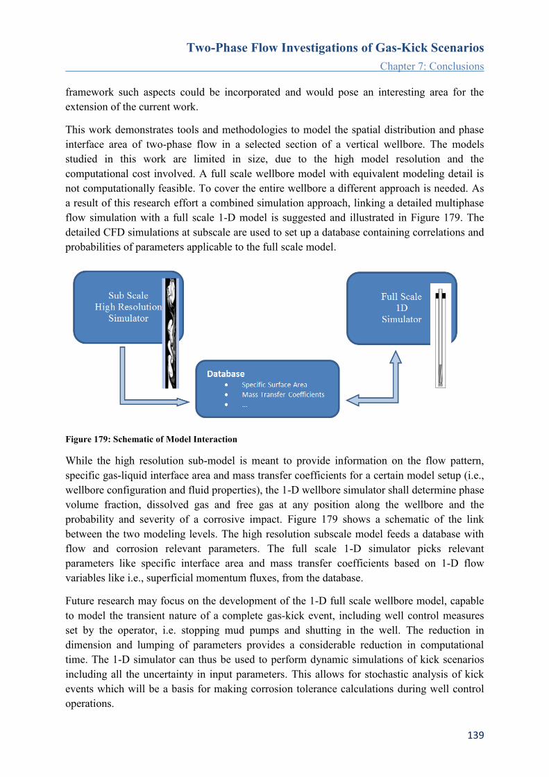
Two-Phase Flow Investigations of Gas-Kick Scenarios
Chapter 7: Conclusions
139
framework such aspects could be incorporated and would pose an interesting area for the
extension of the current work.
This work demonstrates tools and methodologies to model the spatial distribution and phase
interface area of two-phase flow in a selected section of a vertical wellbore. The models
studied in this work are limited in size, due to the high model resolution and the
computational cost involved. A full scale wellbore model with equivalent modeling detail is
not computationally feasible. To cover the entire wellbore a different approach is needed. As
a result of this research effort a combined simulation approach, linking a detailed multiphase
flow simulation with a full scale 1-D model is suggested and illustrated in Figure 179. The
detailed CFD simulations at subscale are used to set up a database containing correlations and
probabilities of parameters applicable to the full scale model.
Figure 179: Schematic of Model Interaction
While the high resolution sub-model is meant to provide information on the flow pattern,
specific gas-liquid interface area and mass transfer coefficients for a certain model setup (i.e.,
wellbore configuration and fluid properties), the 1-D wellbore simulator shall determine phase
volume fraction, dissolved gas and free gas at any position along the wellbore and the
probability and severity of a corrosive impact. Figure 179 shows a schematic of the link
between the two modeling levels. The high resolution subscale model feeds a database with
flow and corrosion relevant parameters. The full scale 1-D simulator picks relevant
parameters like specific interface area and mass transfer coefficients based on 1-D flow
variables like i.e., superficial momentum fluxes, from the database.
Future research may focus on the development of the 1-D full scale wellbore model, capable
to model the transient nature of a complete gas-kick event, including well control measures
set by the operator, i.e. stopping mud pumps and shutting in the well. The reduction in
dimension and lumping of parameters provides a considerable reduction in computational
time. The 1-D simulator can thus be used to perform dynamic simulations of kick scenarios
including all the uncertainty in input parameters. This allows for stochastic analysis of kick
events which will be a basis for making corrosion tolerance calculations during well control
operations.

Two-Phase Flow Investigations of Gas-Kick Scenarios
Chapter 7: Conclusions
140
There is a large requirement for reliable multiphase flow simulators by the oil and gas
industry. Smaller profit margins increase the need for accuracy and planning reliability.
Therefore the demand for a more detailed fluid flow simulation continues to grow. With the
use of CFD flow situations can be investigated where measurements are not available or
experiments are even too difficult to conduct. The design process of new measurement tools
for early kick detection can be supported. In this context Computational Fluid Dynamics is a
valuable tool to validate measurement approaches, i.e. find best measurement locations and
identify key parameters to measure. In general CFD simulations help to better understand and
to review assumptions made about the flow conditions in a kicking well.
Existing wellbore simulators provide good planning assistance but the trend for future
simulators goes to include risk assessment tools as well as real-time data to optimize well
control. Simulators capable to assess the corrosive risk to drilling equipment and to develop
strategies on when to replace drill strings will be needed. Especially when encountering sour
gas (i.e. hydrogen sulfide) influxes into high-pH drilling fluid systems, the prediction of
actual downhole pH development during shut-in and well-killing operations is of prime
interest when deciding on potential damage to high-strength drill string components due to
sulfide stress cracking.
The need for an adequate decision making tool that permits real-time studies of the effects of
risk reducing measures thereby accounting for all the uncertainties involved requires a
probabilistic approach. Stochastic modelling of kick scenarios and the analysis of associated
corrosive damage probability must be based upon a thorough understanding of the physical
phenomena involved. Providing a step towards this fundamental fluid mechanical
understanding, with the help of a highly detailed CFD investigation, was given in this work.

Two-Phase Flow Investigations of Gas-Kick Scenarios
Bibliography
141
Bibliography
Al-Rawajfeh A.E., Modelling and Simulation of CO2 Release in Multiple-Effect Distillers for
Seawater Desalination, PhD thesis, Martin-Luther-Universität Halle-Wittenberg, 2004
Anglart H., Podowski M.Z., Fluid Mechanics of Taylor Bubbles and Slug Flows in Vertical
Channels, Nuclear Science and Engineering, Vol. 140, 2002
ANSYS, Multiphase Flow Conference, HZDR Dresden Rosdorf, Nov. 2015
ANSYS FLUENT, User Guide Manual 14.5, http://www.ansys.com/Products/Fluids/ANSYS-
Fluent, 2015
Barnea D., A unified model for predicting flow-pattern transitions for the whole range of pipe
inclinations, International Journal of Multiphase Flow, Volume 13, Issue 1, 1987
Bendiksen K., Brandt I., Jacobsen K.A., Pauchon C., Dynamic simulation of multiphase
transportation systems, Multiphase Technology and Consequences for Field Development
Forum, Stavanger, Norway, 1987
Bennett A.W., Hewitt G.F., Kearsey H.A., Keeys R.K.F. and Lacey M.P.C., Flow
visualisation studies of boiling at high pressure, Proc. Inst. Mech. Eng., 180 (Part 3C), 1965
Brennen C.E., Fundamentals of Multiphase Flows, Cambridge University Press, 2005
Butterwoth D. and Hewitt G.F., Two Phase Flow and Heat Transfer, Oxford University Press,
1977
Benediksen K.H., Maines D., Moe R., Nuland S., The Dynamic Two-Fluid Model OLGA:
Theory and Application, SPE production Engineering, May 1991
Caetano E.F., Shoham O., Brill J.P., Upward Vertical Two-Phase Flow through an Annulus –
Part I: Single-Phase Friction Factor, Taylor Bubble Rise Velocity, and Flow Pattern
Prediction, Journal Energy Resources Tech., Vol. 114, March, 1-13, 1992
Caetano E.F., Shoham O., Brill J.P., Upward Vertical Two-Phase Flow through an Annulus –
Part II: Modelling Bubble, Slug, and Annular Flow, Journal Energy Resources Tech., Vol.
114, March, 14-30, 1992
Campos J.B.L.M., Guedes de Carvalho J.R.F., An experimental study of the wake of gas slugs
rising in liquids, Journal of Fluid Mechanics, Vol. 196, 1988
Chen L., Tian Y.S., Karayiannis T.G., The effect of tube diameter on vertical two-phase flow
regimes in small tubes, International Journal of Heat and Mass Transfer 49, 2006
Chilingar G.V., Mourhatch R., Al-Qahtani G.D., The Fundamentals of Corrosion and Scaling
for Petroleum & Environmental Engineers, Gulf Publishing Company, 2008
Two-Phase Flow Investigations of Gas-Kick Scenarios
Bibliography
142
Chilingar G.V., Vorabutr P., Drilling and Drilling Fluids, Elsevier Science Ltd, 1981
Clarke A., Issa R. I., Numerical Model of Slug Flow in Vertical Tubes, Computers & Fluids,
Vol. 26(4), 1997
Cussler E.L., Diffusion: Mass Transfer in Fluid Systems, Cambridge University Press, 2009
Duan Z., Sun r., Liu r., Zhu C., Accurate Thermodynamic Model for the Calculation of H2S
Solubility in Pure Water and Brines, Energy & Fuels, 21, 2056 – 2065, 2007
Dukler A.E. and Taitel W., Flow Pattern Transitions in Gas-Liquid Systems: Measurement
and Modelling, Chapter 1 of Multiphase Science and Technology, Vol. 2, Hemisphere
Publishing Corporation, 1986
Fair J.R., What you need to know to design thermosyphon reboilers, Petroleum Refiner 39,
1960
Fernandes R.C., Experimental and Theoretical Studies of Isothermal Upward Gas-Liquid
Flows in Vertical Tubes, Ph.D. Dissertation, University of Houston, Chemical Engineering
Department, 1981
Fraser D., Lindley R., Moore D., Staak M., Early Kick Detection Methods and Technologies,
SPE Annual Technical Conference and Exhibition, Amsterdam, October 2014
Griffith P., Wallis G.B., Two-Phase Slug Flow, ASME, Journal of Heat Transfer, Vol. 83,
1961
Hall-Taylor N.S., Hewitt G.F., Lacey P.M.C., The motion and frequency of large disturbance
waves in annular two-phase flwo of air-water mixtures, Chem. Eng. Sci., 18, 537, 1963
Hewitt G.F., Handbook of Multiphase Systems, Chapter 2, Hemisphere Publishing
Corporation, New York, 1982
Hewitt G.F., Hall-Taylor N., Annular Two-Phase Flow, Oxford: Pergamon Press, 1972
Hewitt G.F., Jayanti S., To Churn or Not To Churn, International Journal of Multiphase Flow,
Vol. 19, No. 3, 1993
Hewitt G.F., King R.D., Lovegrove P.C., Liquid film and pressure drop studies. Chem. Proc.
Eng., 45, 191, 1964
Hewitt G.F., Robertson D.N., Studies of Two-Phase Flow Patterns by Simultaneous X-ray and
Flash Photography, Rept. AERE-M2159, UKAEA, Harwell, 1969
Hibiki T., Ishii M., Two-group interfacial area transport equations at bubbly-to-slug flow
transitions, Nucl. Eng. Des., 202, 39-76, 2000
Hirt C.W., Nichols B.D., Volume of Fluid (VOF) method for the dynamics of free boundaries,
J. Comp Phys, Vol. 39, 1981

Two-Phase Flow Investigations of Gas-Kick Scenarios
Bibliography
143
Hovland F., Rommetveit R., Analysis of Gas-Rise Velocities from Full-Scale Kick
Experiments, 67th Annual Technical Conference and Exhibition of the Society of Petroleum
Engineers, Washington, DC. October 4-7, 1992
Hubbard M.G., Dukler A.E., The characterization of flow regimes for horizontal two-phase
flow: statistical analysis of wall pressure fluctuations, Proceedings of the 1966 Heat Transfer
and Fluid Mechanics Institute, pp. 100–121, 1966
Ishii M., Thermo-fluid dynamic theory of two-phase flow, Collection de la Direction des
Etudes et Researches d’Electricite de France, Eyrolles, Paris, France, 1975
Ishii M., Hibiki T., Thermo-Fluid Dynamics of Two-phase Flow, Springer, New York, USA,
2010
Julia J. E., Hibiki T., Flow regime transition criteria for two-phase flow in a vertical annulus,
International Journal of Heat and Fluid Flow, 32, 2011
Johnson A.B., Cooper S., Gas Migration Velocities During Gas Kicks in Deviated Wells, 68th
Annual Technical Conference and Exhibition of the Society of Petroleum Engineers, Houston,
Texas, 3-6 October 1993
Johnson A. B., White D.B., Gas Rise Velocities During Kicks, SPE 20431, SPE Drilling
Engineer, December 1991
Jones O.C., Zuber N., The Interrelation between Void Fraction Fluctuations and Flow
Patterns in Two-Phase Flow, Int. I. Multiphase Flow, Vol. 2, pp. 273-306, 1975
Kataoka H., Miyauchi T., Gas absorption into the free liquid surface of water tunnel in
turbulent region, Kagaku-Kogaku, 33, pp. 181–186, 1969
Kawaji M. et al., Investigation of Flow Structures in Vertical Slug Flow, Nuclear Engineering
and Design, Vol. 175, 1997
Kreith F., Berger S.A., et al., “Fluid Mechanics”Mechanical Engineering Handbook, Ed.
Frank Kreith, Boca Raton: CRC Press LLC, 1999
Mao Z.S., Dukler, A. E., The Motion of Taylor Bubbles in Vertical Tubes. I. A Numerical
Simulation for the Shape and Rise Velocity of Taylor Bubbles in Stagnant and Flowing
Liquid, Journal of Computational Physics, Vol. 91, 1990
McQuillan K.W., Whalley P.B., Flow Patterns in Vertical Two-Phase Flow, International
Journal of Multiphase Flow, Vol. I 1, No. 2, 1985
O’Brien T.B., Handling Gas in an Oil Mud Takes Special Precautions, World Oil, 1981
OLGA: https://www.software.slb.com/products/olga
Owen, D.G., An experimental and theoretical analysis of equilibrium annular flows, Ph.D.
Thesis, University of Birmingham, UK, 1986
Two-Phase Flow Investigations of Gas-Kick Scenarios
Bibliography
144
Ozar B., Jeong J.J., Dixit A., Juliá J.E., Hibiki T., Ishii M., Flow structure of gas-liquid two-
phase flow in an annulus, Chemical Engineering Science 63, p. 3998-4011, 2008
Pauchon C., Dhulesia H., Lopez D., Fabre J., TACITE: A comprehensive mechanistic model
for two-phase flow, Proceedings of the 6th International Conference on Multiphase
Production, Cannes, France, 1993
Pauchon C., Dhulesia H., Binh-Cirlot G. and Fabre J., TACITE: A transient tool for
multiphase pipeline and well simulation, SPE Annual Technical Conference, New Orleans,
LA, USA, 1994
Pilliod J.E., Puckett E.G., Second-order accurate volume-of-fluid algorithms for tracking
material interfaces, Journal of Computational Physics, Vol. 199, 2004
Rommetveit R., Olsen T.L., Gas Kick Experiments in Oil-Based Drilling Muds in a Full-
Scale, Inclined Research Well, SPE 19561, 64th Annual Technical Conference and Exhibition
of the Society of Petroleum Engineers, San Antonio, TX, October 8-11, 1989
Schicht, H.H., Flow patterns for an adiabatic two-phase flow of water and air within a
horizontal tube, Verfahrenstechnik, 3, No.4, 1969
Schmidtke M., Untersuchung der Dynamik fluider Partikel auf Basis der Volume of Fluid
Methode, Dissertation, Department Chemie, Universität Paderborn, 2009
Serizawa A., Kataoka I., Phase Distribution in Two-Phase Bubbly Flow, ICHMT Int. Sem.
Transient Two-Phase Flow, Dubrovnik, Yugoslavia, 177, 1987
Shyy W., Udaykumar H.S., Rao M.M., Smith R. W., Computational Fluid Dynamics with
Moving Boundaries, Taylor & Francis, Bristol, Pennsylvania, 1996
SINTEF Flow Loops, website: www.sintefloops.com
Srinivasan S., Kane R., Prediction of corrosivity of CO2/H2S production environments, NACE
International Corrosion Conferenc & Expo, 1996
Stenberg O., Andersson B., Gas-liquid mass transfer in agitated vessels - II. Modelling of
gas-liquid mass transfer, Chem. Eng. Sci. 1988; 43: 725-730.
Sun W., Nesic S., A mechanistic model of H2S corrosion of mild steel, NACE International
Corrosion Conference & Expo, 2007
Taha T., Cui Z.F., CFD modelling of slug flow in vertical tubes, Chemical Engineering
Science, Vol. 61, 2006
Taitel Y., Advances in Two Phase Flow Mechanistic Modeling, University of Tulsa
Centennial Petroleum Engineering Symposium, Tulsa, Oklahoma, August 1995
Taitel Y., Barnea D. and Dukler A.E., Modeling Flow Pattern Transitions for Steady Upward
Gas-Liquid Flow in Vertical Tubes, AIChE Journal 26, no. 6, May 1980

Two-Phase Flow Investigations of Gas-Kick Scenarios
Bibliography
145
Taitel Y., Dukler A.E., A model for prediction flow regime transitions in horizontal and near
horizontal gas–liquid flow, AIChE Journal 22, 1976
Thermopedia: A-to-Z Guide to Thermodynamics, Heat and Mass Transfer, and Fluids
Engineering, Begellhouse, Digital Library, 2006
Tong L.S. and Tang Y.S., Boiling Heat Transfer and Two Phase Flow, CRC Press, 1997
Ubbink O., Numerical prediction of two fluid systems with sharp interfaces, Dissertation,
Department of Mechanical Engineering, Imperial College of Science, London University,
1997
Viana F., Pardo R., Ýanez R., Trallero J., Joseph D., Universal correlation for the rise
velocity of long gas bubbles in round pipes, Journal of Fluid Mechanics, Vol. 494, 2003
Waclawczyk T., Koronowicz T., Modeling of the flow in systems of immiscible fluids using
Volume of Fluid method with CICSAM scheme, Turbulence, Vol. 8, 2005
Wallis G.B., One dimensional two phase flow, McGraw-Hill, New York, 1969
Wang S., Nesic S., On coupling CO2 Corrosion and Multiphase Flow Models, Corrosion
2003, Paper No. 03631
Weisman J., Duncan D., Gibson J., Crawford T., Effects of fluid properties and pipe diameter
on two-phase flow patterns in horizontal lines, International Journal of Multiphase Flow 5,
1979
Weisman J., Kang S., Flow pattern transitions in vertical and upwardly inclined lines,
International Journal of Multiphase Flow 7, 1981
Whalley P.B., Two Phase Flow and Heat Transfer, Oxford University Press, 1996
Whalley P.B., Boiling and Condensation and Gas-Liquid Flow, Clarendon Press,
Oxford, 1987http://dx.doi.org/10.1017/S0022112088211739
Xiaodong Z., Mechanistic-based models for slug flow in vertical pipes, Dissertation, 2005
Youngs D.L., Time-dependent multi-material flow with large fluid distortion. In: Morton
K.W., Baibnes M.J. (Eds.), Numerical Methods for Fluid Dynamics. Academic Press, New
York, p. 273, 1982
Zheng L., Yapa P.D., Chen F., A model for simulating deepwater oil and gas blowouts – Part
I: Theory and model formulation, Journal of Hydraulic research, Vol. 41, No. 4, 2002
Zuber N., Findlay J.A., Average volumetric concentration in two phase flow system, ASME,
Journal of Heat Transfer, Vol. 87, 1965