Two-level non-parametric scaling for

dichotomous data

Tom A.B. Snijders

ICS/Department of Statistics and Measurement Theory

University of Groningen ∗

Abstract

It is relevant to extend the existing single-level scaling methods to two-level designs. Examples are the scaling of teachers on the basis of theirpupils’ responses, or scaling neighborhoods on the basis of responses byinhabitants. A non-parametric approach is convenient because it requiresfew assumptions and leads to easy calculations.

This paper considers a two-level situation where the objects to be scaledare the higher level units; nested within each object are lower level units,called ‘subjects’; a set of dichotomous items is administered to each subject.A two-level version is elaborated of the non-parametric scaling method firstproposed by Mokken (1971). The probabilities of positive responses to theitems are supposed to be increasing functions of the value on a latenttrait; this value is composed of a subject-dependent value and a deviationfrom this value due to the object and the subject-object interaction. Thissituation may be viewed as one with strictly parallel tests that are definedby the objects.

Loevinger H coefficients are defined to assess the consistency of re-sponses within, but also between objects. The availability of parallel testsis used to calculate coefficient alpha to assess the reliability of the scale.Keywords: Multi-level models, item response theory, non-parametricscaling, reliability, parallel tests, ecometrics.

∗Department of Statistics and Measurement Theory, Grote Kruisstraat 2/1, 9712 TS Gronin-gen, The Netherlands, email t.a.b.snijders@ppsw.rug.nl, http://stat.gamma.rug.nl/snijders/ .

1

1 Introduction

In item response theory we are accustomed to situations where the subjects who

provide the responses are also the objects which are to be measured; more gen-

erally, where for each individual to be scaled exactly one set of item responses is

available. There are situations, however, where these roles are fulfilled by distinct

entitities, as is demonstrated by the following examples.

1. Pupils are asked questions about their teachers, with the purpose to assess

the teachers (as perceived by the pupils) on a certain dimension.

2. Employees are asked to respond to a questionnaire about the department

they work in, in order to scale the departments with respect to working

climate.

3. Social settings such as neigborhoods are assessed by a survey of multiple

informants (e.g., inhabitants). The answers given by the informants are

aggregated to provide an assessment of the social setting (Raudenbush and

Sampson, 1998, use the term ecometrics for such an approach).

4. In a study of personal networks, for each respondent (‘ego’) in a survey, a

list is made of the other persons (‘alters’) to whom the respondent is related

according to certain criteria. A number of characteristics of the alters are

collected in order to characterize ego’s social environment (Jansson and

Spreen, 1998).

The objects to be measured in these examples are, respectively, teachers, de-

partments, social settings, and respondents. For each object a set of multiple

measurements is available: multiple pupils, employees, informants, and alters.

These units will be called subjects, although this word may be unexpected in

the fourth example. Each of the multiple measurements is supposed to yield a

vector of responses to the same set of items. This defines a three-level nesting

structure: responses denoted Yijk to items k are nested within subjects j, which

in their turn are nested within objects i. Equivalently, this can be regarded as a

multivariate two-level nesting structure, where subjects are nested within objects

and each subject provides a vector of responses Yij = (Yij1, ..., YijK).

The purpose of the analysis is to give scale values to the objects, while the

subjects are regarded as parallel tests of these objects. It will be assumed that

the item responses Yijk are dichotomous, scored as 1 (‘positive’, ‘correct’) and 0

(‘negative’, ‘false’). The statistical approach elaborated here is a non-parametric

2

latent trait model in the sense that a one-dimensional latent trait is assumed

to govern (stochastically) the item responses, and the assumptions about how

the response probabilities depend on the latent trait are of a qualitative nature

only and do not restrict these probabilities to a particular mathematical function.

Relevant questions are the following:

• What is, in this two-level design, a suitable non-parametric definition of the

relation between latent trait and observed responses?

• How to assess empirically whether indeed there is a one-dimensional latent

variable which underlies the responses to the items?

• How can the objects be scored on this latent dimension?

• What is the reliability of the resulting scale?

These questions will be answered by elaborating a two-level version of the non-

parametric scaling method first proposed by Mokken (1971) and explained and

elaborated by Mokken and Lewis (1982), Mokken (1997), and Molenaar and

Sijtsma (200?). Alternative parametric models are also available for this two-

level scaling design, as will be mentioned in the Discussion.

The Mokken scaling model is an attractive non-parametric model for uni-

dimensional cumulative scaling. This model can be summarized as follows. Sub-

jects, to be indexed by the letter i, respond to dichotomously scored items indexed

by the letter k. The response (scored 0 or 1) of object i to item k is denoted

Yik. It is assumed that a latent trait θ exists for which each person has a value,

denoted θi, determining the probability distribution of i′s vector of responses.

Further it is assumed that for each item k, there exists a non-decreasing function

pk(.) such that the probability of a positive response, given the latent trait value

θi, is

P {Yik = 1 | θi} = pk(θi) . (1)

These functions pk(.) are called tracelines, or item characteristic curves. Further-

more, the Mokken model assumes local stochastic independence: conditional on

the value of the latent trait, the responses of the subject are outcomes of inde-

pendent random variables. Important questions in the application of this scaling

method are the scalability of a given set of items, the selection of a scalable subset

from a given set of items, and the attribution of scores to subjects. Procedures for

data analysis according to this model are described in the literature mentioned

above, and implemented in the program MSP.

3

2 A two-level model for non-parametric

scaling of dichotomous data

As stated above, Yijk denotes the response of subject j to item k with regard to

object i. The set of items scored for each object-subject combination is assumed

to be constant, while the number of subjects may vary between objects. The

number of subjects providing responses with regard to object i is denoted ni.

The model elaborated for this situation is a cumulative scaling model governed

by a uni-dimensional latent trait θ. We assume that for each object i there is a

value θi on the latent trait, and to each subject j nested within object i there

corresponds a deviation δij from this value. Combined, this yields the combined

value θi + δij as the resultant value on the latent trait for the combination of

subject j and object i. The deviation δij may be considered as a (random)

subject effect together with object by subject interaction. Conditional on these

latent trait values, we assume stochastic independence of the responses to the

different items and subjects. We also assume the existence of tracelines pk(.)

that are specific to the items but do not depend on object or subject, and that

are non-decreasing, and give the probabilities of positive responses:

P{Yijk = 1 | θi, δij} = pk(θi + δij) . (2)

Further, we assume that all subjects providing data for the objects are a random

sample from some population of subjects. The parallel tests therefore are inde-

pendent, conditionally on θi. For the statistical model this means that the δij are

independent and identically distributed random variables.

In terms of multilevel analysis (as treated by Bryk and Raudenbush, 1992;

Goldstein, 1995; Snijders and Bosker, 1999), this may be regarded as a model

where the random parts at levels two and three are composed of random intercepts

without random slopes.

In Section 5 we treat the question of defining object scores in order to scale the

objects. Scaling object i amounts in this model to estimating a suitable monotone

increasing function of θi. (This function is defined below by (21); in this non-

parametric framework the latent parameter θi itself is not identifiable, because no

assumptions are made as to the shape of the tracelines; also see Mokken, 1971).

When var(θi) is large compared to var(δij), then the differences between the

subjects hardly matter compared to the differences between the objects. This is

desirable from the point of view of scaling the objects. When, on the contrary,

var(θi) is small compared to var(δij), then the probabilities of the two responses

4

to the items are determined by the subjects rather than by the objects, leading

to a comparatively unreliable test (unless the number of subjects per object is

large).

It follows from this model that the marginal probability of a positive response

for a randomly drawn subject to object i is

πk(θi) = P{Yijk = 1 | θi} = Eδ pk(θi + δij) , (3)

where the expectation Eδ refers to the distribution of δij. The function πk(.)

inherits from the function pk(.) the property of being monotone non-decreasing.

(The property of double monotonicity, defined in the following section, is also

inherited by πk(.) from pk(.).) However, the function πk(.) will be flatter than

the original traceline pk(.), because of the process of averaging with respect to

the distribution of δij.

The questions concerning this model treated in this paper are the following:

• Model adequacy: do the items together form a cumulative scale which

is suitable for scaling the objects? This is investigated on the basis of

Loevinger scalability coefficients.

• The definition of scores for objects.

• The reliability of the resulting scale.

3 Scalability coefficients

In the usual form of Mokken scaling, scalability coefficients are defined as follows.

These coefficients are based on a further assumption, namely, the assumption of

double monotonicity: the items k are ordered in such a way, that

p1(θ) ≤ p2(θ) ≤ . . . ≤ pm(θ) for all θ,

where K is the number of items. For item pairs k, k′ with k < k′, the responses

Yik, Yik, are said to form an error if Yik = 1 while Yik′ = 0, contradicting

the expected ordering. For the definition of the scalability coefficients it is also

assumed that objects have been drawn at random from some population, or that

(more loosely) the θi values for the objects can be considered to be represen-

tative for some population. This assumption is needed because the scalability

coefficients are defined relative to the marginal joint probability distribution of

the item scores, i.e., the distribution of (Yi1, Yi2, . . . , YiK) for a randomly drawn

5

object; these coefficients depend jointly on the items and the population of ob-

jects. Loevinger’s H coefficients of scalability can now be defined (see Mokken,

1971 and Mokken and Lewis, 1982) with respect to each item pair (k < k′) as

one minus the ratio of the probability of an error response for the item pair to

the same probability under the null model of independent item responses,

Hkk′ = 1− P{Yik = 1, Yik′ = 0}P{Yik = 1}P{Yik′ = 0}

.

In the case of a perfect Guttman scale this scalability coefficient equals 1, in

the case of independent (unrelated) items this coefficient equals 0. A similar

coefficient can be defined for each item, by considering the total number of errors;

note that for item k, pattern Yik′ = 1, Yik = 0 forms an error if k′ < k, while

pattern Yik = 1, Yik′ = 0 forms an error if k′ > k. The H coefficient for item

k is accordingly defined by

Hk = 1 −

k−1∑k′=1

P{Yik′ = 1, Yik = 0} +K∑

k′=k+1P{Yik = 1, Yik′ = 0}

k−1∑k′=1

P{Yik′ = 1}P{Yik = 0} +K∑

k′=k+1P{Yik = 1}P{Yik′ = 0}

.

Similarly, the H coefficient for the whole scale is based on the total number of

errors:

H = 1−∑k<k′ P{Yik = 1, Yik′ = 0}∑

k<k′ P{Yik = 1}P{Yik′ = 0}.

It is useful to note here that the scalability coefficients are completely deter-

mined by the tracelines pk(.) together with the probability distribution in the

object population of the latent trait values θi. The h coefficients are higher, in

general, when tracelines are steeper and when the object distribution has greater

dispersion. The scalability coefficients should not be regarded as indicators of

unidimensionality as such, but rather as indicators of how well the given set

of items performs in assigning unidimensional scale values to objects from the

population under study.

These notions can be adapted to our two-level design. We wish to know how

well each object i can be measured by the set of responses Yijk (k = 1, ..., K; j =

1, ..., ni). It is to be expected that responses given by the same subject are more

consistent, i.e., contain less errors, than responses given by different subjects.

Accordingly, we distinguish within-subject scalability coefficients from between-

subject scalability coefficients, where the former are expected to be higher than

the latter.

6

For item pairs k < k′, the within-subject scalability coefficient is defined as

HWkk′ = 1 − P{Yijk = 1, Yijk′ = 0}

P{Yijk = 1}P{Yijk′ = 0}, (4)

where attention must be given the fact that a single subject j is considered. The

between-subject scalability coefficient is defined as

HBkk′ = 1 − P{Yijk = 1, Yij′k = 0}

P{Yijk = 1}P{Yijk′ = 0}(j 6= j′) , (5)

where two different subjects j and j′ are considered in the numerator. (Since

the denominator is the product of two separate probabilities not depending on j,

replacing the last j in the denominator by a j′ would not make any difference.)

Analogous scalability coefficients for the items are the within-subject scala-

bility coefficient

HWk = 1−

k−1∑k′=1

P{Yijk′ = 1, Yijk = 0} +K∑

k′=k+1P{Yijk′ = 0, Yijk = 1}

k−1∑k′=1

P{Yijk′ = 1}P{Yijk = 0} +K∑

k′=k+1P{Yijk = 1}P{Yijk′ = 0}

(6)

and the between-subject scalability coefficient

HBk = 1−

k−1∑k′=1

P{Yij′k′ = 1, Yijk = 0} +K∑

k′=k+1P{Yij′k′ = 0, Yijk = 1}

k−1∑k′=1

P{Yijk′ = 1}P{Yijk = 0}+K∑

k′=k+1P{Yijk = 1}P{Yijk′ = 0}

.(7)

For the entire scale, the within-subject scalability coefficient is defined by

HW = 1 −∑k<k′ P{Yijk = 1, Yijk′ = 0}∑

k<k′ P{Yijk = 1}P{Yijk′ = 0}, (8)

and the between-subject scalability coefficient by

HB = 1 −∑k<k′ P{Yijk = 1, Yij′k′ = 0}∑

k<k′ P{Yijk = 1}P{Yijk′ = 0}(j 6= j′). (9)

The within-subject scalability coefficients refer to the situation that the two

levels are combined (or ‘disaggregated’) by considering every object-subject com-

bination as a single case. In other words, they are the usual H coefficients for

scalability of the items for object-subject combinations treated as independent

replications. The probabilities in the definitions of the within-subject scalabil-

ity coefficients are determined by the tracelines pk(.) and the distribution of the

latent parameter values θi + δij, e.g.,

P{Yijk = 1, Yijk′ = 0} = EθEδ {pk(θi + δij)(1− pk′(θi + δij))} . (10)

7

The between-subject scalability coefficients, on the other hand, are coefficients

for scalability of the objects when the items are responded to by different, i.e.,

independent subjects. The probabilities in their definitions are determined by

the tracelines πk(.) given in (3) and the distribution of the objects’ latent trait

values θi, as is expressed in

P{Yijk = 1, Yij′k′ = 0} = Eθ {πk(θi)(1− πk′(θi))}. (11)

Since the tracelines πk(.) are flatter than pk(.), and the distribution of θi + δij is

more dispersed than that of θi, the within-subject scalability coefficients must be

greater than between-subject scalability coefficients, unless the deviations δij are

constant, in which case they are equal. This is indeed proven in the appendix.

Thus, it holds that 0 ≤ HB ≤ HW . Suppose that var(θi + δij) > 0 and the

tracelines are strictly increasing; then HW > 0. In the extreme situation that

var(δij) = 0, it holds that 0 < HB = HW . In the extreme situation that var(θi) =

0 we have 0 = HB < HW , and, scaling of objects makes no sense.

For the investigation of the quality of the scale as a unidimensional cumulative

scale for object-subject combinations, the within-subject scalability coefficients

are the most relevant. Their interpretation is similar to the interpretation of

scalability coefficients in the usual Mokken scaling model. In the usual Mokken

scaling procedure, a value of 0.3 is considered a low value for scalability, while

0.5 is good (e.g., Mokken and Lewis, 1982). In the present two-level situation,

however, within-subject scalability coefficients may be allowed to be lower than

0.3, because of the presence of several subjects per object.

For the investigation of the degree to which the object value on the latent

trait, θi, determines the responses to the items, the between-subject scalability

coefficients, and their relation to within-subject coefficients, provide useful in-

formation. The discussion given above about the relation between HB and HW

implies that the ratio HB/HW can be used as an indication of between-to-within-

subject variability of the latent parameter. When HB is almost as large as HW ,

then the responses for the object are hardly affected by the particular subject

(the influence of the random deviation δij is small); when, on the contrary, HB

is much smaller than HW , then the responses for the object are strongly affected

by the particular subject (the influence of δij is large). Similar interpretations

can be attached to the ratios HBkk′/H

Wkk′ and HB

k /HWk . Relatively small values of

the between-subject coefficients imply that a large number of subjects (or items)

is necessary for a reliable estimation of object scores. Very small values of the

between-subject coefficients suggest that the object parameter θi is perhaps not

8

a very relevant parameter because its influence on the responses to the items is

small compared to the influence of the subjects, expressed by the deviations δij.

Another way to assess the effect of the random subjects is to compute within-

object and between-object covariance matrices of the items. These covariance

matrices are, like the scalability coefficients, based on the probabilities of the item

responses and of joint responses to pairs of items. The within-object correlation,

which can be computed from these covariance matrices, shall be considered in

Section 4.

4 Estimation of the scalability coefficients

The various scalability coefficients can be estimated by taking the defining for-

mulae amd substituting relative frequencies for the probabilities. Recall that the

number of subjects presented to object i is ni; define the total number of sub-

jects presented by n+, and the total number of objects by N . We assume that

the frequencies ni are stochastically independent of the random variables Yijk,

conditional on the latent trait values θi and δij; we shall see that it is not a big

problem if the ni are correlated with the latent trait values θi.

If the numbers ni are not the same for all i, then there are two ways to

estimate the probabilities in formulas (4) to (9). We discuss their difference for

the probabilities P{Yijk = 1}. The first way is to average the relative frequencies

for all objects:

P{Yijk = 1} =1

N

∑i

1

ni

∑j

Yijk . (12)

The other way is to average the frequencies for the objects:

P{Yijk = 1} =1

n+

∑i

∑j

Yijk . (13)

To understand the difference between these two estimators, note that the prob-

ability P{Yijk = 1} is defined by

P{Yijk = 1} = EθEδ P{Yijk = 1 | θi, δij} = EθEδ pj(θi + δij) ,

where the subscripts θ and δ indicate that the expectation is taken with respect

to the corresponding random variables. The probability for object i,

P{Yijk = 1 | θi} = EδijP{Yijk = 1 | θi, δij} ,

9

is estimated unbiasedly by the relative frequency for object i,

P{Yijk = 1 | θi} =1

ni

∑j

Yijk .

This demonstrates that (12) defines an unbiased estimator, even if there is a

stochastic dependence between ni and θi.

Since estimator (13) weighs the individual relative frequencies by ni/n+, the

latter estimator is unbiased only if the ”sample sizes” ni and the latent trait

values θi are stochastically independent. Since this assumption is not always

warranted, we opt for estimator (12). This estimator shall be denoted Pk.

The estimators for the probabilities of error patterns, analogous to (12), are

PWk,k′(1, 0) = P{Yijk = 1, Yijk′ = 0} =

1

N

∑i

1

ni

∑j

Yijk(1− Yijk′) (14)

and

PBk,k′(1, 0) = P{Yijk = 1, Yij′k′ = 0} =

1

N

∑i

1

ni(ni − 1)

∑j 6=j′

Yijk(1−Yij′k′).(15)

Substitution of these estimators leads to the following estimators of the scalability

coefficients:

HWkk′ = 1−

PWk,k′(1, 0)

Pk(1− Pk′), (16)

HBkk′ = 1−

PBk,k′(1, 0)

Pk(1− Pk′), (17)

HW = 1−∑k<k′ P

Wk,k′(1, 0)∑

k<k′ Pk(1− Pk′), (18)

HB = 1−∑k<k′ P

Wk,k′(1, 0)∑

k<k′ Pk(1− Pk′), (19)

and similarly for HWk and HB

k .

As a final remark it can be added that if disaggregated data, i.e., data where

object-subject combinations are treated as independent replications, are used

as input in the MSP program for Mokken scaling, then the scalability coeffi-

cients computed are the within-subject coefficients, but with estimates analogous

to (13), and therefore weighted by ni/n+. If all ni are equal, then this is correct.

If the ni values are considerably different from each other, however, while they

are correlated with the latent trait values θi, this approach can yield incorrect

results.

10

5 Object scores

Object scores can be defined as

Y i.. =1

mni

∑j,k

Yijk. (20)

Each index over which has been averaged is replaced by a dot. Just like in the

usual Mokken model, these object scores are not estimators for θi, because the

non-parametric nature of the model makes it impossible to estimate these latent

values: they are not identifiable. The expectation of Y i.. is

µ(θi) =1

m

m∑k=1

πk(θi), (21)

a monotone function of θi. So, apart from chance fluctuations, the relation be-

tween Y i.. and θi is monotone. Of course the standard error of estimation of Y i..

depends on ni as well as on θi.

6 Reliability

For the usual Mokken scaling method, there are several methods to estimate

reliability; these methods of estimation are based on the matrix of joint posi-

tive responses to pairs of items, the so-called P matrix, see Mokken (1971) and

Sijtsma and Molenaar (1987). A nice feature of our two-level design is the avail-

ability of independent within-object replications. These replications imply that a

within-object between-subject test-retest correlation coefficient can be estimated

as the intra-class correlation coefficient, where classes are defined by the objects.

Define σ20 as the variance of average scores for randomly drawn object-subject

combinations,

σ20 = var(Y ij.) .

Further define the within-object between-subject correlation

ρ = corr(Y ij., Y ij′.) =1

σ20

cov(Y ij., Y ij′.) (j 6= j′) ;

then ρ can be regarded as the intra-class correlation coefficient, where classes are

defined by the objects. This parameter will be called the intra-object correlation

coefficient. The variance of the object score for a random object with ni subjects

is

var (Y i..) =σ2

0

ni{1 + (ni − 1)ρ} . (22)

11

To define estimators for σ20 and ρ, denote the average object score by

Y ... =1

N

N∑i=1

Y i.. ;

note that Y ... is not the mean of all Yijk values, but the mean of the object

scores Y i..; these two means are the same if all the ni are equal. Further, denote

between-object and within-object variances by

S2B =

1

N − 1

N∑i=1

(Y i.. − Y ...)2

and

S2W =

1

N

N∑i=1

1

(ni − 1)

ni∑j=1

(Y ij. − Y i..)2 .

(The weights 1/(ni−1) are used in order to let S2W be the average of the observed

within-object variances; since the object variances are not necessarily the same,

this is the only way to get an unbiased estimator for the expectation of the

theoretical covariance for a randomly drawn object.) Define the harmonic mean

ν of the ni by

1

ν=

1

N

N∑i=1

1

ni.

It can be proved straightforwardly that

E(S2W ) = σ2

0(1− ρ)

and

E(S2B) =

σ20

ν{1 + (ν − 1)ρ} .

This yields the estimators

σ20 =

ν − 1

νS2W + S2

B (23)

ρ =1

σ20

{S2B −

1

νS2W} . (24)

The estimated intra-object correlation ρ is the test-retest reliability for the par-

allel tests corresponding to the different subjects. The test-retest correlation for

12

two independent scores Y i.. for the same object i (obtained from two indepen-

dent sets each consisting of ni independent subjects) is the well-known reliability

coefficient known as coefficient alpha (see, e.g., Nunnally, 1967, p. 193)

ρ(Y i.., Y′i..) =

niρ

(ni − 1)ρ+ 1=

niρ

niρ+ 1− ρ. (25)

This reliability coefficient will be very important in the final assessment of the

quality of the scale for objects, as an addition to the Loevinger scalability coeffi-

cients treated in Section 3.

7 Examples for simulated data

The presentation of some results for simulated data may give a better under-

standing of the various parameters introduced and the numerical values these

may assume. Three data sets were generated for N = 500 objects, each con-

fronted with ni= 10 subjects for which K = 6 items were scored. The tracelines

of the items satisfied the Rasch model (see, e.g., Fischer and Molenaar, 1995):

pk(θ) =exp(θ − ξk)

1 + exp(θ − ξk),

where ξk is the difficulty parameter of item k. The difficulty parameters were

chosen as -2.0, -1.2, -0.4, 0.4, 1.2, 2.0. The distributions of θi and δij were normal

with mean 0.

The three simulated data sets differed according to the ratio of within-subject

to between-subject variances: the variances were σ2θ = 0.5, σ2

δ = 0.5 (simulation

1), σ2θ = 0.8, σ2

δ = 0.2 (simulation 2), and σ2θ = 0.2, σ2

δ = 0.8 (simulation 3).

Thus, the variance of the combined latent trait values θi + δij is in all three cases

equal to 1. This implies that the item popularities (marginal probabilities of a

positive response) and the within-subject H coefficients are the same in the three

simulations.

For simulation 1, where the variance of object values for the latent trait is

equal to the variance of the subject-related deviations, the popularities and scal-

ability coefficients were estimated as presented in Tables 1, 2 and 3.

We see, what is well known for Mokken scaling, that H coefficients are greater

when the item popularities are further apart. Further, the between-subject H

coefficients are indeed considerably smaller than the within-subject coefficients.

13

Table 1: Estimated item probabilities for simulated data set 1.

k 1 2 3 4 5 6

Pk 0.158 0.266 0.409 0.577 0.734 0.842

Table 2: Estimated within-subject scalability coefficients

for simulated data set 1.

HWkk′ k′ 1 2 3 4 5 6

k

1 — 0.138 0.210 0.349 0.411 0.432

2 — 0.155 0.283 0.309 0.452

3 — 0.212 0.290 0.401

4 — 0.221 0.278

5 — 0.182

6 —

Items

k 1 2 3 4 5 6

HWk 0.253 0.227 0.231 0.253 0.256 0.301

Whole scale

HW 0.250

14

Table 3: Estimated between-subject scalability coefficients

for simulated data set 1.

HBkk′ k′ 1 2 3 4 5 6

k

1 — 0.067 0.098 0.195 0.164 0.182

2 — 0.078 0.137 0.147 0.188

3 — 0.113 0.104 0.135

4 — 0.086 0.111

5 — 0.075

6 —

Items

k 1 2 3 4 5 6

HBk 0.121 0.108 0.102 0.120 0.103 0.118

Whole scale

HB 0.111

Table 4: Estimated values for coefficient alpha for simulated data set 1.

ni 4 8 10 20 30

ρ(Y i.., Y i..′) 0.549 0.709 0.753 0.859 0.901

15

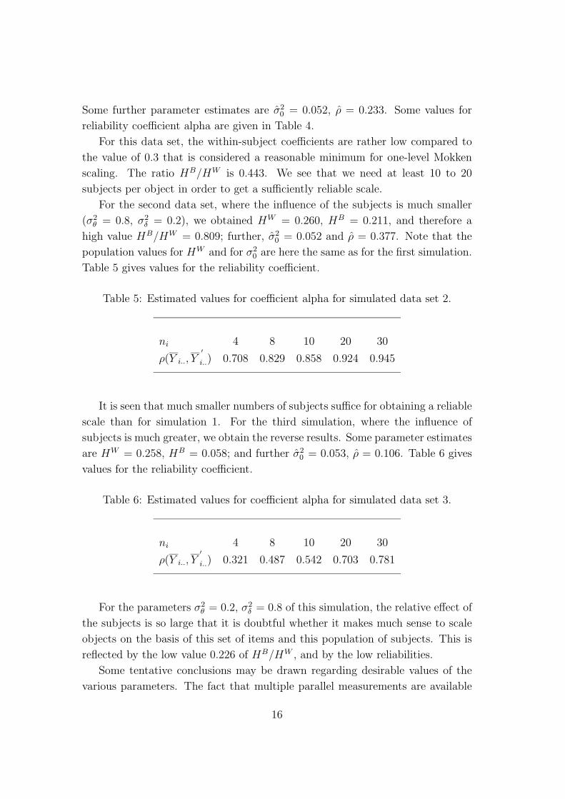
Some further parameter estimates are σ20 = 0.052, ρ = 0.233. Some values for

reliability coefficient alpha are given in Table 4.

For this data set, the within-subject coefficients are rather low compared to

the value of 0.3 that is considered a reasonable minimum for one-level Mokken

scaling. The ratio HB/HW is 0.443. We see that we need at least 10 to 20

subjects per object in order to get a sufficiently reliable scale.

For the second data set, where the influence of the subjects is much smaller

(σ2θ = 0.8, σ2

δ = 0.2), we obtained HW = 0.260, HB = 0.211, and therefore a

high value HB/HW = 0.809; further, σ20 = 0.052 and ρ = 0.377. Note that the

population values for HW and for σ20 are here the same as for the first simulation.

Table 5 gives values for the reliability coefficient.

Table 5: Estimated values for coefficient alpha for simulated data set 2.

ni 4 8 10 20 30

ρ(Y i.., Y′

i..) 0.708 0.829 0.858 0.924 0.945

It is seen that much smaller numbers of subjects suffice for obtaining a reliable

scale than for simulation 1. For the third simulation, where the influence of

subjects is much greater, we obtain the reverse results. Some parameter estimates

are HW = 0.258, HB = 0.058; and further σ20 = 0.053, ρ = 0.106. Table 6 gives

values for the reliability coefficient.

Table 6: Estimated values for coefficient alpha for simulated data set 3.

ni 4 8 10 20 30

ρ(Y i.., Y′

i..) 0.321 0.487 0.542 0.703 0.781

For the parameters σ2θ = 0.2, σ2

δ = 0.8 of this simulation, the relative effect of

the subjects is so large that it is doubtful whether it makes much sense to scale

objects on the basis of this set of items and this population of subjects. This is

reflected by the low value 0.226 of HB/HW , and by the low reliabilities.

Some tentative conclusions may be drawn regarding desirable values of the

various parameters. The fact that multiple parallel measurements are available

16

allows the use of scales with lower H values than in single-level nonparametric

scaling still having a satisfactory reliability. Within-subject scalability coefficients

for items and for the whole scale should be greater than 0.2 for a good scale; it

is not serious if for some directly consecutive item pairs, the HWkk′ coefficient

is between 0.1 and 0.2. The consistency between subjects is satisfactory when

between-subject homogeneity coefficients are at least 0.1 (with possibly some

exceptions for between-item HBkk′ coefficients). For the ratio HB/HW , values

over 0.3 are reasonable and values over 0.6 are excellent. As indicators for the

quality of the scale one should use not only the homogeneity coefficients, but also

coefficient alpha for practical ni values.

8 Example: assessment of teachers by pupils

In a study by Bosker and others (1999), pupils in primary schools were asked to

respond to a questionnaire about their teacher and classroom. As an example,

some questions about the classroom climate and order are used. Six items from

the questionnaire were selected on the basis of face value considerations (mainly

their unambiguous relation to order in the class). The items are statements with

three answer categories (‘true’, ‘somewhat true’, ‘not true’). They were recoded

to values 1, 2, 3, where 1 denotes the most orderly and 3 the most chaotic situation

in the classroom. A cross-validatory approach was chosen in which the first phase

used data for group-6 pupils (age 9–10 years) for the selection of a good subset

of items and dichotomization thresholds, and the second phase used the data for

group-7 pupils (age 10–11 years) for the evaluation of the resulting scale along

the lines of the preceding sections.

In the first phase, items and thresholds were chosen – in a trial and error

procedure – so as to yield relatively high between-subject H coefficients for each

item. This resulted in a scale of four items, all dichotomized by contrasting the

values 1 and 2 (most and intermediate orderly, coded as Y = 0) with the value

3 (least orderly, coded as Y = 1). The four items are the following. They are

ordered in increasing frequency of the least orderly outcome.

1. When the teacher tells us something, we listen well (inversely coded).

2. It is usually quiet in the classroom (inversely coded).

3. There often is much noise in the classroom.

4. The teacher often tells us to be quiet.

17

These items were subjected to a scale analysis for the group-7 pupils (whose

data were not used in the selection of items and thresholds) as the second phase

of the data analysis. There were data for 1530 pupils (subjects) and 77 class-

rooms/teachers (objects). The results are presented in Tables 7 to 10.

Table 7: Estimated item probabilities for classroom climate scale.

k 1 2 3 4

Pk 0.062 0.277 0.351 0.524

Table 8: Estimated within-subject scalability coefficients

for classroom climate scale.

HWkk′ k′ 1 2 3 4

k

1 — 0.697 0.740 0.676

2 — 0.562 0.555

3 — 0.556

4 —

Items

k 1 2 3 4

HWk 0.707 0.576 0.578 0.566

Whole scale

HW 0.587

The between-to-within subject ratio of the scalability coefficient for the entire

scale is HB/HW = 0.367. The intra-object correlation is ρ = 0.258.

It can be concluded that this four-item scale is very satisfactory. Within-

subject pairwise H coefficients are 0.55 and higher, between-subject pairwise H

coefficients are 0.18 and higher. The consistency of response within and also be-

tween subjects is large enough to use these four questions for assessing classroom

18

Table 9: Estimated between-subject scalability coefficients

for classroom climate scale.

HBkk′ k′ 1 2 3 4

k

1 — 0.324 0.324 0.396

2 — 0.179 0.204

3 — 0.201

4 —

Items

k 1 2 3 4

HBk 0.343 0.207 0.204 0.220

Whole scale

HB 0.215

Table 10: Estimated values for coefficient alpha for for classroom climate scale.

ni 4 8 10 20 30

ρ(Y i.., Y′

i..) 0.582 0.736 0.777 0.874 0.913

19

climate. About 10 pupils are sufficient to give a reasonably reliable measurement

instrument.

9 Discussion

A non-parametric method has been presented to scale objects who are known to

the researcher only through responses which refer to subjects connected in some

way to the objects. The subjects, nested within the objects, are supposed to be

a random sample from a population, and a test composed of dichotomous items

is administered to each object-subject combination. This makes for a two-level

data structure.

The consistency of answer patterns within subjects can be measured by within-

subject Loevinger H coefficients applied to the disaggregated object-subject com-

binations. To scale the objects on the basis of such data requires, however, that

there is enough consistency also between the subjects in their answer patterns.

This is measured by between-subject Loevinger H coefficients.

To investigate how well the objects are scaled by this set of items, two mea-

sures have been presented: the ratio HB/HW of between-subject (within-object)

to within-subject scalability coefficients, which gives an indication of the extent

to which scale values are determined by objects rather than by subjects (and

object-subject interactions); and coefficient alpha for the reliability of the result-

ing scale. Coefficient alpha depends, of course, on the number of subjects per

object.

Scales for objects defined in this way can be used, e.g., to investigate relations

between the corresponding latent trait and other variables referring to the objects,

such as the relation between classroom climate and teacher behavior, or the

relation between neighborhood climate and policy instruments applied to the

neighborhoods.

A possible alternative to the non-parametric approach presented here is a

parametric three-level model for dichotomous data, where the levels are items,

subjects, and objects. A standard approach, elaborated for the three-level case

by Gibbons and Hedeker (1997), is to assume normal distributions for the latent

trait components θi and δij, and a logistic link function for the dichotomous

responses. Although this may be called a standard approach from the point

of view of model building, the numerical calculations necessary to estimate the

parameters are very complicated. Reviews of parametric models for multilevel

dichotomous data (but with a focus on two-level models) are given by Goldstein

20

(1995, Chapter 7) and Snijders and Bosker (1999, Chapter 14). Such an approach

yields the rewards connected to the richer parametric structure: the possibility of

using covariates for subjects and/or objects, the availability of standard statistical

methods such as maximum likelihood to obtain estimates and standard errors.

However, for these models the estimation methods are numerically quite complex

and computationally demanding. Moreover, the parametric assumptions will

often be questionable; the logistic link function means that one assumes the

Rasch model for the object-subject combinations, and the Rasch model is known

to be quite a strong assumption for a cumulative unidimensional scale.

Advantages of the non-parametric method presented here are the light as-

sumptions and the easy computations. A PC program to carry out the calcula-

tions is available from the web site http://stat.gamma.rug.nl/snijders/multilevel.htm .

A Appendix. Proof that between-subject scala-

bility coefficients are not larger than within-

subject coefficients.

It shall be proved that

P{Yijk = 1, Yijk′ = 0} ≤ P{Yijk = 1, Yij′k′ = 0} (j 6= j′) . (26)

This is equivalent with HBkk′ ≤ HW

kk′ , and it implies HBk ≤ HW

k and HB ≤ HW .

To prove (26), note that

P{Yijk = 1, Yij′k′ = 0} − P{Yijk = 1, Yijk′ = 0}= (P{Yijk = 1} − P{Yijk = 1, Yij′k′ = 1})− (P{Yijk = 1} − P{Yijk = 1, Yijk′ = 1})

= P{Yijk = 1, Yijk′ = 1} − P{Yijk = 1, Yij′k′ = 1} .

From the expressions analogous to (10) and (11) we can conclude that this equals

Eθ Eδ {pk(θi + δij)pk′(θi + δij)} − Eθ {πk(θi)πk′(θi)}= Eθ [Eδ {pk(θi + δij)pk′(θi + δij) | θi} − πk(θi)πk′(θi)] .

Because of the definition of πk, given in (3), this is equal to

Eθ [covδ{pk(θi + δij), pk′(θi + δij) | θi}] .

21

The conditional covariance,

covδ{pk(θi + δij), pk′(θi + δij) | θi} ,

is a covariance of two non-decreasing functions of the random variable δij. Such

a covariance is always non-negative, which proves (26). If the tracelines pk(.) are

strictly increasing and var(δij) > 0, then this covariance is strictly positive, so

that the strict inequality HWkk′ > HB

kk′ holds.

In a similar way it can be proved that

P{Yijk = 1, Yij′k′ = 0} − P{Yijk = 1}P{Yijk′ = 0}= − covθ {πk(θi), πk′(θi)} ≤ 0 ,

which implies HBkk′ ≥ 0.

References

Bosker, R.J., and others (1999), Zelfevaluatie in het basisonderwijs (ZEBRA).

University of Twente.

Fischer, G.H., and Molenaar, I.W. (1995), Rasch Models. Foundations, Recent

Developments, and Applications. New York: Springer.

Gibbons, R.D., and Hedeker, D. (1997), Random effects probit and logistic re-

gression models for three-level data. Biometrics, 53, 1527–1537.

Goldstein, H. (1995), Multilevel Statistical Models, 2nd ed. London: Edward

Arnold.

Jansson, I., and Spreen, M. (1998), The use of local networks in a study of heroin

users: assessing average local networks. Bulletin de Methodologie Soci-

ologique, 59, 49–61.

Mokken, R.J. (1971), A theory and procedure of scale analysis. The Hague: Mou-

ton.

Mokken, R.J. (1971), Nonparametric models for dichotomous responses, pp. 351–

367 in W.J. van der Linden and R.K. Hambleton (eds.), Handbook of Modern

Item Response Theory, New York: Springer.

Mokken, R.J., and Lewis, C. (1982), A nonparametric approach to the analysis

of dichotomous item responses, Applied Psychological Measurement, 6, 417–

430.

Molenaar, W., and Sijtsma, K. (200?). Textbook on non-parametric scaling.

Nunnally, J.C. (1967), Psychometric Theory. New York: MacGraw-Hill.

22

Raudenbush, S.W., and Bryk, A.S. (1992), Hierarchical Linear Models, New-

bury Park: Sage.

Raudenbush, S.W., and Sampson, R.J. (1998), ”Ecometrics”: Toward a science

of assessing ecological settings, with applications to the systematic social

observatiopn of neigborhoods. Paper under review.

Sijtsma, K., and Molenaar, I.W. (1987), Reliability of test scores in nonparamet-

ric item response theory, Psychometrika, 52, 79–97.

Snijders, T.A.B., and Bosker, R.J. (1999), Multilevel Analysis. An Introduction

to Basic and Advanced Multilevel Modeling. London: Sage.

23