two innovative applications combining fiber optics and
TRANSCRIPT

Two Innovative Applications Combining Fiber Optics and High Power
Pulsed Laser: Active Ultrasonic Based Structural Health Monitoring and
Guided Laser Micromachining
Chennan Hu
Dissertation submitted to the faculty of the Virginia Polytechnic Institute and State
University in partial fulfillment of the requirements for the degree of
Doctor of Philosophy
In
Physics
Anbo Wang, Co-Chair
James R. Heflin, Co-Chair
Chenggang Tao
Hans Robinson
February 15, 2017
Blacksburg, Virginia
Keywords: Engineering, Electronics and Electrical
Physics, Optics
Physics, Acoustics
Copyright 2017, Chennan Hu

Two Innovative Applications Combining Fiber Optics and High Power Pulsed
Laser: Active Ultrasonic Based Structural Health Monitoring and Guided Laser
Micromachining
Chennan Hu
ABSTRACT This dissertation presents the exploration of two fiber optics techniques involving high power pulse laser
delivery. The first research topic is “Embedded Active Fiber Optic Sensing Network for Structural Health
Monitoring in Harsh Environments”, which uses the fiber delivered pulse laser for acoustic generation.
The second research topic is “Fiber Optics Guided Laser Micromachining”, which uses the fiber delivered
pulse laser for material ablation.
The objective of the first research topic is to develop a first-of-a-kind technology for remote fiber optic
generation and detection of acoustic waves for structural health monitoring in harsh environments. Three
different acoustic generation mechanisms were studied in detail, including laser induced plasma
breakdown (LIB), Erbium-doped fiber laser absorption, and metal laser absorption. By comparing the
performance of the acoustic generation units built based on these three mechanisms, the metal laser
absorption method was selected to build a complete fiber optic structure health monitoring (FO-SHM)
system. Based on the simulation results of elastic wave propagation and fiber Bragg grating acoustic pulse
detection, an FO-SHM sensing system was designed and built. This system was first tested on an
aluminum piece in the room temperature range and successfully demonstrated its capability of multi-
parameter monitoring and multi-point sensing. With additional studies, the upgraded FO-SHM element
was successfully demonstrated at high temperatures up to 600oC on P-91 high temperature steels.
During the studies of high power pulse laser delivery, it was discovered that with proper laser-to-fiber
coupling, the output laser from a multimode fiber can directly ablate materials around the fiber tip.
Therefore, it is possible to use a fiber-guided laser beam instead of free space laser beams for
micromachining, and this solves the aspect ratio limitation rooted in a traditional laser beam
micromachining method. In this dissertation, this Guided Laser MicroMachining (GLMM) concept was
developed and experimentally demonstrated by applying it to high aspect ratio micro-drilling. It was
achieved that an aspect ratio of 40 on aluminum and an aspect ratio of 100 on PET, with a hole diameter
less than 200 µm.

Two Innovative Applications Combining Fiber Optics and High Power Pulsed
Laser: Active Ultrasonic Based Structural Health Monitoring and Guided Laser
Micromachining
Chennan Hu
General Audience Abstract
This dissertation presents two research topics both related to high power laser and fiber optic. The first
topic studies the application of using optical fiber and high power laser for ultrasonic non-destructive
evaluation. The general idea is to use fiber optic to remotely generate and monitor ultrasonic waves on a
workpiece. Due to the fact that there are no electronic components involved in the sensing part of the
system, this system can work at high temperature and is unsusceptible to EMI. The second topic studies
the usage of optical fiber in high aspect ratio micromachining. The key concept is to use a fiber tip and
the output high power laser as a “drilling tip”, which eliminate the aspect ratio limitation rooted in the
traditional free-space laser micromachining method. With this concept and a demonstrative
micromachining system, we achieved record-breaking aspect ratio on both aluminum and plastic.

iv
Acknowledgement
First of all, I want to thank my parents who raised me and supported me all the way through my
education. Without their love and caring I would not be who I am today.
I want to thank my advisor Dr. Anbo Wang. It is some great effort Dr. Wang has put in to maintain
such a wonderful lab: the Center for Photonics Technology (CPT), where I had access to all types of
equipment and opportunities to learn from many amazing people. Dr. Wang himself is wise, kind
and patient. He gave me good advice when I faced a problem and encouraged me when I made
progress. Most importantly, he put great trust in me and gave me enough freedom in conducting
research. I also receive helps from other committee members during my study so I want to thank
them: Dr. Randy Heflin, Dr. Hans Robinson and Dr. Chenggang Tao.
I want to thank all my fellow labmates in CPT who have given me helps and made my life easier:
Zhihao Yu, Cheng Ma, Dorothy Wang, Kathy Wang, Michael Fraser, Peng Lv, Guo Yu, Tyler
Shillig, Scott Zhang, Lingmei Ma, Zhipeng Tian, Di Hu, Li Yu, Bo Liu, Amiya Behera, Shuo Yang
and Jiaji He. A special thank you to Bo Dong, who has been a great mentor in the lab and also a
loyal friend.
I want to thank my lovely fiancee Keren for her company in this great small town Blacksburg. We
have enjoyed wonderful life here fishing, snowboarding and doing lots of other activities outside our
labs. This will be a forever memorable six years for us two.
Last but not the least, I want to thank all the sponsors of my research projects including the National
Energy and Technology Laboratory (NETL) of the Department of Energy (DOE), the National
Science Foundation (NSF) and General Electric (GE).

v
Table of Contents
Table of Contents .......................................................................................................................................... v
List of Figures and Tables ............................................................................................................................ ix
1 Introduction to the fiber optic structure health monitoring (FO-SHM) ................................................ 1
2 Study of the laser induced plasma (LIP) based acoustic generation ..................................................... 3
2.1.1 Experimental comparison of the opto-acoustic conversion efficiency between thermal
expansion and LIP ................................................................................................................................. 3
Demonstration of single point LIP based acoustic generation and detection ............................... 6
Multiplexable LIP and FBG based FO-SHM element design, fabrication and test .................... 10
Conclusion .................................................................................................................................. 16
3 Test and comparison of two thermal expansion based acoustic generation schemes ......................... 17
Erbium-doped fiber (EDF) based acoustic generation ................................................................ 17
Scattering light&metal absorption based acoustic generation .................................................... 18
Experimental comparison ........................................................................................................... 21
Analysis of opto-acoustic conversion efficiency ........................................................................ 25
Conclusion .................................................................................................................................. 27
4 Simulations of the ultrasonic pulse based multi-parameter monitoring scheme ................................. 28
FEM simulation of crack and corrosion detection using the elastic wave model ....................... 28
4.1.1 Simulation model building in COMSOL ............................................................................ 30
4.1.2 Simulation result ................................................................................................................. 31

vi
Temperature induced acoustic velocity change calculation ........................................................ 35
Simulation of fiber Bragg grating (FBG) response to short acoustic pulse ................................ 37
4.3.1 The transfer matrix method ................................................................................................. 38
4.3.2 Simulation result ................................................................................................................. 40
5 The design and demonstration of an all fiber optic structural health monitoring system ................... 41
System design and operation procedure ...................................................................................... 41
Experimental setup ...................................................................................................................... 42
FO-SHM node installation and acoustic signature analysis ........................................................ 45
Multi-parameter monitoring demonstration of a single FO-SHM node ..................................... 49
5.4.1 Strain monitoring ................................................................................................................ 49
5.4.2 Thickness monitoring .......................................................................................................... 51
5.4.3 Temperature monitoring ..................................................................................................... 52
5.4.4 Crack detection ................................................................................................................... 54
Demonstration of multiplexed FO-SHM monitoring .................................................................. 56
Conclusion .................................................................................................................................. 59
6 High temperature FO-SHM element surface attachment design, simulation, and test ....................... 60
Identifying the structure health monitoring target material ........................................................ 60
Numerical simulation of thermal stress on surface attached FO-SHM sensor ........................... 61
High temperature test of surface attached FO-SHM elements (ceramic adhesive) .................... 65
6.3.1 The first surface attachment method ................................................................................... 65

vii
6.3.2 The second surface attachment method .............................................................................. 71
Low CTE metallic adhesive based FO-SHM sample high temperature test ............................... 75
Type-II FO-SHM components fabrication and high temperature test ........................................ 84
7 High temperature FO-SHM system demonstration ............................................................................. 88
Step one - high temperature tests using standard optical fiber .................................................... 88
7.1.1 High temperature tests with standard 105/125m fiber ...................................................... 89
7.1.2 High temperature tests with silver coated 105/125μm fiber ............................................... 91
Step two - high temperature tests using gold coated optical fiber .............................................. 96
Step three - high temperature tests using FP-FBG sensing structure ........................................ 100
7.3.1 Principle of FP-FBG ......................................................................................................... 100
7.3.2 High temperature test results ............................................................................................. 102
Corrosion, strain and crack tests ............................................................................................... 105
7.4.1 Corrosion test .................................................................................................................... 105
7.4.2 Strain test .......................................................................................................................... 107
7.4.3 Crack test .......................................................................................................................... 109
Conclusions ............................................................................................................................... 111
8 Guided elastic wave study for future research .................................................................................. 113
Analytical model of guided elastic wave propagation .............................................................. 113
FEM simulation of the guided elastic wave and experimental result ....................................... 114
9 Introduction to fiber optic guided laser micromachining (GLMM) .................................................. 118

viii
10 Simulations of the GLMM process ............................................................................................... 120
Modelling the shape of a static “drilling tip” ............................................................................ 120
Dynamic simulation of the GLMM drilling process ................................................................. 121
11 Experimental setup and results ..................................................................................................... 123
Experimental setup .................................................................................................................... 123
Drilling results on aluminum .................................................................................................... 124
Drilling results on PET ............................................................................................................. 128
12 Conclusions to the fiber optic guided laser micromachining ........................................................ 129
13 Dissertation summary ................................................................................................................... 131
Reference: ................................................................................................................................................. 132

ix
List of Figures and Tables
Figure 2-1 Experimental setup to test the opto-acoustic converting efficiency of LIP and thermal
expansion process ......................................................................................................................................... 4
Figure 2-2 Experimental result of the opto-acoustic converting efficiency for the LIP process and the
thermal expansion process ............................................................................................................................ 5
Figure 2-3. Demonstrative optical fiber LIP acoustic generating unit. ......................................................... 6
Figure 2-4. Demonstrative FBG acoustic detection unit design (a) and the fabricated unit (b). .................. 7
Figure 2-5. System setup of the single point acoustic generation and detection demonstration. .................. 8
Figure 2-6. Reflection spectrum of the FBG used in the acoustic detector. ................................................. 8
Figure 2-7. Comparison of the experimental result (solid blue line) and the simulation result (dashed red
line). .............................................................................................................................................................. 9
Figure 2-8. Preliminary FO-SHM unit demonstration test: (a) acoustic generation and detection units
directly attached; (b) acoustic wave passes through copper rod before detected by FBG ............................ 9
Figure 2-9. Signals acquired with the demonstrative FO-SHM unit: (a) 1064nm laser pulse; (b) acoustic
signal acquired with FBG unit directly attached to acoustic generation unit; (c) acoustic signal acquired
with FBG unit and acoustic generation unit separated by a piece of 40cm-long copper rod ...................... 10
Figure 2-10. Structure of multiplexing in-fiber LIP acoustic generating units. .......................................... 11
Figure 2-11. Fabrication of a demonstrative LIP based FO-SHM element. ............................................... 12
Figure 2-12. LIP unit test setup and unit breakage ..................................................................................... 13
Figure 2-13. Microscope images of the two fiber ends taken after the unit broke: (a) the fiber with the well
for the metal layer and (b) the mating fiber ................................................................................................ 14
Figure 2-14. Image of the metal coated fiber end before spliced with the mating fiber ............................. 14
Figure 2-15. Improved splicing of the second LIP FO-AGU ..................................................................... 15

x
Figure 2-16. Acoustic signal generated by the second LIP unit and detected by a PZT detector in water . 16
Figure 3-1 Level diagram of Er3+ in EDF[17] ............................................................................................. 17
Figure 3-2. Design of an EDF based FO-SHM element ............................................................................. 18
Figure 3-3. Standard multimode fiber + standard single mode fiber .......................................................... 19
Figure 3-4. Un-doped double cladding fiber (DCF) ................................................................................... 20
Figure 3-5. Twin-core fiber ......................................................................................................................... 20
Figure 3-6. AGU test scheme with a PZT as the acoustic detector ............................................................. 21
Figure 3-7. Experimental setup of the EDF based FO-SHM system: (a) acoustic generation system using a
980nm pulsed laser; (b) test bench .............................................................................................................. 22
Figure 3-8. (a) Driving signal and (b) measured laser output power of the 980nm pulsed laser ................ 23
Figure 3-9. (a) AGU made with 4mm section of SMF-28e with scattering voids inscribed by a
femtosecond laser; (b) AGU made with 40cm coiled EDF (Thorlabs ER80-8/125) .................................. 24
Figure 3-10. Acoustic signals generated by the scattering-based and EDF-based AGUs .......................... 24
Figure 4-1. Simulation specimen geometry. ............................................................................................... 31
Figure 4-2. Simulation results of elastic wave propagation trace in a specimen with a crack. ................... 32
Figure 4-3. Simulation results of crack-induced acoustic signals. .............................................................. 33
Figure 4-4. Simulation results of corrosion-induced acoustic signals. ....................................................... 34
Figure 4-5. (a) The ratio of the sound velocity at temperatures from 0-1000°C to the sound velocity at
20°C; (b) the ratio of the fly time variance at temperatures from 0-1000°C to the acoustic wave
propagating distance ................................................................................................................................... 36
Figure 4-6. While a slow acoustic pulse (a) passes through an FBG, the instantaneous stress will be
indicated by a shift in its reflection spectrum (b). The reflection intensity of a laser with its wavelength
fixed on one edge of the main peak will be modulated in response to the stress wave (c). ........................ 37

xi
Figure 4-7. The reflection response of a 1.5mm long FBG to a 32ns (0.16mm long in space) acoustic
pulse. Red line: acoustic pulse. Blue line: simulated FBG response signal. ............................................... 40
Figure 5-1 (a) System schematic of an FO-SHM system; (b) Sample spectrum of an FO-SHM system
containing 5 nodes ...................................................................................................................................... 41
Figure 5-2 Simplified pulse laser optical fiber coupling scheme with CCD imaging system .................... 43
Figure 5-3 (a)Free-space laser to optical fiber coupling system; (b)Fiber core alignment method ............ 44
Figure 5-4 Preliminary experiment setup .................................................................................................... 44
Figure 5-5 (a) FO-SHM node installed on the tested aluminum plate; (b) optical fiber special splicing
structure; (c) pre-installation test with EFPI fiber sensor and direct laser illumination. ............................ 46
Figure 5-6 (a) Acoustic signatures obtained with EFPI sensor and direct laser surface illumination, the
shift of each curve represents the source-receiver distance; (b) Acoustic signatures obtained with FBG
sensor and direct laser surface illumination, the shift of each curve represents the source-receiver distance;
(c) The final acoustic signature of the FO-SHM unit and its related acoustic signatures from the two pre-
installation tests. .......................................................................................................................................... 48
Figure 5-7 Strain test setup ......................................................................................................................... 50
Figure 5-8 (a) FBG spectrum monitoring during the strain change process; (b) FBG peak location shifts
caused by the strain changes. ...................................................................................................................... 50
Figure 5-9 Milling off sample bottom to simulate the corrosion ................................................................ 51
Figure 5-10 (a) Acoustic signatures in the thickness monitoring test; (b) peak #T1 center shift; (c) peak
#B center shift; (d) peak #T2 center shift. .................................................................................................. 52
Figure 5-11 (a) Acoustic signatures in the temperature monitoring test; (b) peak #T1 center shift; (c) peak
#B center shift; (d) peak #T2 center shift. .................................................................................................. 53
xii
Figure 5-12 (a) FBG spectrum monitoring during the temperature change process; (b) FBG peak location
shifts caused by the temperature changes. .................................................................................................. 54
Figure 5-13 (a) FO-SHM sample with a machined slot on it; (b) Comparison of the original acoustic
signature and acoustic signature with a machined slot on the sample. ....................................................... 55
Figure 5-14 PLB test result with the FO-SHM element ............................................................................. 56
Figure 5-15 Type-II voids for acoustic generation ..................................................................................... 57
Figure 5-16 Sample for multiplexed FO-SHM system demonstration ....................................................... 58
Figure 5-17 LabVIEW controlling software for the multiplexed FO-SHM system ................................... 59
Figure 6-1 P91 pipes purchased for the FO-SHM system demonstration................................................... 61
Figure 6-2. Simulation model. .................................................................................................................... 62
Figure 6-3. Mesh for FEM analysis. ........................................................................................................... 63
Figure 6-4. Von-Mises stress of the whole model. ..................................................................................... 64
Figure 6-5. (a) Von-Mises stress on the tube; (b) Strain along the fiber axis; (c) Top view of Von-Mises
stress distribution on the adhesive; (d) Bottom view of Von-Mises stress distribution on the adhesive. ... 65
Figure 6-6. FO-SHM element surface attached to a P91 pipe by high temperature ceramic adhesive. ...... 66
Figure 6-7 Surface attached FO-SHM element after the high temperature test .......................................... 67
Figure 6-8 Ceramic adhesive after heating up to 300o C ............................................................................ 67
Figure 6-9 Signal of the surface attached FO-SHM element at different temperature points ..................... 68
Figure 6-10 FBG spectrum during the second high temperature test ......................................................... 69
Figure 6-11 (a) Simulation model with surface attached FBG heated to 600o C; (b,c) Non-uniform strain
distribution along the silica fiber; (d) Simulation result of FBG spectrum with non-uniform strain. ......... 70
Figure 6-12 New schematic of FO-SHM element embedment ................................................................... 72
Figure 6-13 COMSOL simulation result of thermal strain distribution at 200o C ...................................... 72

xiii
Figure 6-14 Full embedment sample preparation and new large volume tube furnace used in the test ..... 73
Figure 6-15 FBG spectrums during the temperature changing process ...................................................... 74
Figure 6-16 New FO-SHM embedment plan .............................................................................................. 76
Figure 6-17 Experiment setup for AE signature acquisition on a P91 pipe with EFPI sensor and direct
laser illumination acoustic generation ......................................................................................................... 77
Figure 6-18 AE signatures acquired in the first test set .............................................................................. 78
Figure 6-19 Fabrication process and experiment setup for FBG + direct illumination FO-SHM sample .. 79
Figure 6-20 AE signatures at different distance between excitation point and detection point .................. 79
Figure 6-21 Completed state of the FO-SHM node on a P91 pipe ............................................................. 80
Figure 6-22 (a) AE signature for FBG and direct illumination; (b) AE signature for the completed FO-
SHM sensing node ...................................................................................................................................... 81
Figure 6-23 FBG spectrum during high temperature test ........................................................................... 82
Figure 6-24 Acoustic signatures during the high temperature test, intensities calibrated by their relating
FBG intensities............................................................................................................................................ 83
Figure 6-25 FFT information of the acoustic signatures during the high temperature test ......................... 84
Figure 6-26 (a) The Libra femtosecond laser; (b) The point-by-point type-II FBG inscription system. .... 86
Figure 6-27 (a) Type-II FBG spectrum; (b) The periodical structure of the type-II FBG under 100X
microscope. ................................................................................................................................................. 86
Figure 6-28 Surface attached type-II FBG high temperature test result ..................................................... 87
Figure 6-29 Type-II voids constructed acoustic generation unit................................................................. 88
Figure 7-1 P-91 sample with type-II FO-NDE elements ............................................................................ 89
Figure 7-2 Acoustic signature evolution in high temperature environment ................................................ 90
Figure 7-3 Fiber light leakage after a high temperature test ....................................................................... 91

xiv
Figure 7-4 Silver coating fiber sputter setup ............................................................................................... 92
Figure 7-5 Acoustic generation unit on silver coated fiber ......................................................................... 92
Figure 7-6 (a) Light leakage at 300oC; (b) Light leakage at 600oC. ........................................................... 93
Figure 7-7 Overall view of the acoustic signature evolution with silver coated fiber ................................ 94
Figure 7-8 Zoom-in view of the front section of the acoustic signature evolution ..................................... 95
Figure 7-9 (a) P-91 high temperature test sample with gold coated fiber FO-NDE element attached; (b)
Sample in the furnace; (c) FO-NDE element remains in good shape after heating; (d) Acoustic generation
unit on a gold coated fiber; (d) Acoustic generation unit attachment on the P-91 pipe. ............................. 97
Figure 7-10 Acoustic signature evolution during the high temperature test. .............................................. 98
Figure 7-11 (a) FBG spectrums during a high temperature test; (b) FBG peak reflectance evolution; (c)
FBG peak wavelength evolution. .............................................................................................................. 100
Figure 7-12 Principle of the FP-FBG acoustic sensing ............................................................................. 102
Figure 7-13 P-91 test sample prepared with FP-FBG for acoustic sensing .............................................. 102
Figure 7-14 (a) FP-FBG spectrum evolution during a high temperature test; (b) Peak reflectance evolution;
(c) Peak wavelength evolution. ................................................................................................................. 103
Figure 7-15 Acoustic signature evolution during a high temperature test ................................................ 104
Figure 7-16 (a) Pipe inner surface electro-etching setup; (b) Acoustic signature evolution during the
corrosion process ...................................................................................................................................... 105
Figure 7-17 Strain test setup ..................................................................................................................... 107
Figure 7-18 Strain test results ................................................................................................................... 108
Figure 7-19 PLB signal ............................................................................................................................. 109
Figure 7-20 Crack simulation setup and cut sample ................................................................................. 110
Figure 7-21 Crack test results ................................................................................................................... 110

xv
Figure 8-1 Dispersion curves for symmetric Lamb waves (red curves), anti-symmetric Lamb waves (blue
curves) and SH waves (green curves) ....................................................................................................... 114
Figure 8-2 COMSOL simulation result of elastic wave generation by laser heating ............................... 115
Figure 8-3 Experiment setup for thin-wall tube elastic wave generation and detection ........................... 116
Figure 8-4 Results comparison between the COMSOL simulation result and the experimental result .... 117
Figure 9-1 Key principle of optical fiber guided micro drilling and side hole debris flushing ................. 119
Figure 10-1 Simulation result of the cross-section shape of a "drilling tip" with different boundaries; the
value on each boundary represents the normalized laser intensity on that boundary relative to the laser
intensity in the fiber core; surrounding medium is water with refractive index. (a) Simulation result of the
dependent relationships of drilling ratio and bottom clearance on fiber NA (b) Simulation result of the
dependent relationships of drilling ratio and bottom clearance on the relative in-fiber laser intensity .... 121
Figure 10-2 Simulation results of different drilling conditions, minimum ablation rate of the static
“drilling tip” ARmin=0.54μm/pulse, maximum ablation rate ARmax=1.25μm/pulse. (a) VD >ARmax, hole
formation stops at certain depth (b) ARmin<VD <ARmax , hole diameter stabilized at certain depth (c)
VD <ARmin , uniform hole diameter at all depth = the diameter of the static “drilling tip”. .................. 123
Figure 11-1 Schematic of the GLMM based high aspect ratio micro hole drilling system. ..................... 124
Figure 11-2 (a) Setting initial gap; (b) Drilling starts; (c) Fiber tip enters the hole; (d) Drilling deeply
inside the hole; (e) Drilling completed. .................................................................................................... 125
Figure 11-3 Aluminum drilling results. (a) AR=8 hole with bare fiber for comparison; (b) Fiber tip before
and after the drilling process; (c) AR=15 hole; (d) AR=40 hole drilled on the side wall. ........................ 126
Figure 11-4 The depth progression and LIP intensity record of the drilling process. ............................... 127
Figure 11-5 (a) Drilling debris observation under surface profiler; (b) Side wall surface roughness
measurements by surface profiler. ............................................................................................................ 128

xvi
Figure 11-6 AR=125 PET drilling results ................................................................................................. 129
Table 1 Equipment used for thermal expansion based acoustic generation methods comparison .............. 22
Table 2. Material properties ........................................................................................................................ 26
Table 3 Simulation model properties .......................................................................................................... 31
Table 4. Propagation speed of the elastic waves in 7075 aluminum .......................................................... 46
Table 5. Curve fitting results of the three peaks and the expected values .................................................. 47
Table 6. Peak location associated response rates to temperature change .................................................... 53
Table 7 Properties of each section .............................................................................................................. 58
Table 8 Material properties for thermal stress simulation .......................................................................... 63
Table 9 Typical type-II FBG inscription parameters .................................................................................. 85
Table 10 Parameters used for the inscription of the acoustic generation type-II voids .............................. 87

1
1 Introduction to the fiber optic structure health monitoring (FO-SHM)
The interconnected consequences of the national energy strategy compel us to design energy systems to
operate at higher temperatures to achieve greater efficiency from fossil fuel systems with lower
greenhouse gas emissions. One example is the Ultra Supercritical (USC) steam cycle design, which
raises the operating steam temperature to 760oC for an efficiency target of 45-47% and a 25-30%
reduction in CO2 emissions [1]. Another is the Integrated Gasification Combined Cycle (IGCC) by which
coal can be chemically broken down into syngas products at temperatures well above 1000oC [2]. The
gaseous and solid products of the IGCC process exhibit minimal waste of coal while minimizing carbon
emission. Such progressive energy systems, which operate at temperatures much higher than traditional
fossil fuel power plants, present a new set of extreme physical and chemical conditions such as ultra-high
temperatures, high pressure, and severe chemical corrosion. Materials directly exposed to these harsher
environments tend to suffer significant physical or chemical degradation. It is thus indispensable to
monitor the health condition of key materials and structures involved in these systems in real time to
ensure safety and minimize system shutdowns [3].
Currently available means of assessing material or structural health include on-site assessment methods
such as X-ray defect detection [4] and ultrasonic tomography [5], and remote techniques which
commonly use piezoelectric acoustic transducers. The first methods are reliable and accurate but require
on-site access which is often prohibited due to the harsh environments involved in the energy systems.
The remote techniques have been effective for structural health monitoring and are often applied to civil
structures, however, they are generally restricted to applications at temperatures below 500oC [6, 7].
Although high temperature piezoelectric transducers have been actively investigated for more than a
decade, their reliability at high temperatures still remains a major concern [7-9]. In addition, like other

2
electrical sensors, they are susceptible to electromagnetic interference (EMI). Their signal can also be
transmitted through wireless modules, but on-site electric power is required which often presents
additional maintenance issues. Given this situation, it is therefore imperative to develop new techniques
which allow on-site maintenance-free monitoring of the health conditions of the critical materials and
structures that are used in high temperature applications and other harsh environments.
In this research, we developed a new Fiber Optics Structure Health Monitoring (FO-SHM) technology for
multi-parameter measurement by realizing fiber optic generation and detection of acoustic waves. A
single FO-SHM element is constructed with a pair of in-fiber acoustic generation/detection units, which
have a low physical profile (less than 300 um in width). The FO-SHM element is surface attached to the
material under monitoring, imposing a minimal intrusion to the integrity of the structure. The detected
acoustic signature and the returned optical spectrum allow extraction of information about material’s
condition including temperature, strain, corrosion, and defects, such as cracks and delamination, which
can challenge the structure integrity. In addition, the FO-SHM element can be operated at temperatures
well above 800oC if not mounted and up to 600oC in the current surface attachment scheme. This
technology is also able to monitor multiple locations with serially connected FO-SHM elements and a
single interrogation system for long span structure monitoring.

3
2 Study of the laser induced plasma (LIP) based acoustic generation
In this section, the laser induced breakdown mechanism, also known as laser induced plasma (LIP), is
studied for its possible application in fiber optics based acoustic generation. The mechanisms of laser-
induced acoustic wave excitation include electrostriction, thermal expansion, photochemical changes, gas
evolution, and breakdown of plasma formation [10]. Among all these mechanisms, Laser Induced Plasma
(LIP) formation breakdown has the highest opto-acoustic conversion efficiency, which can reach around
30% [11]. On the other hand, conventional thermal expansion only has a conversion efficiency in the
order of 10-12 to 10-8 [10]. Studies show that LIP can generate strong acoustic shock wave in both the
water confined geometry and glass confined geometry with a fast temporal response to the laser pulse [12,
13].
2.1.1 Experimental comparison of the opto-acoustic conversion efficiency between
thermal expansion and LIP
In this section, we presented a test to compare the opto-acoustic generation efficiency between the LIP
process and the thermal expansion process. A free space laser beam was focused onto the surface of an
aluminum sample to excite acoustic vibration on the sample either through thermal expansion or laser
induced plasma breakdown, depending on the laser intensity. A PZT transducer attached on the aluminum
sample recorded the acoustic signal. The relationship between the laser energy density and the acoustic
intensity was then plotted to show the difference in opto-acoustic converting efficiency for LIP and
thermal expansion process. As shown in Figure 2-1, a Nd:YAG pulsed laser with 50ns pulse width was
used as the acoustic excitation laser, and the illuminated spot is about 1mm2.
4
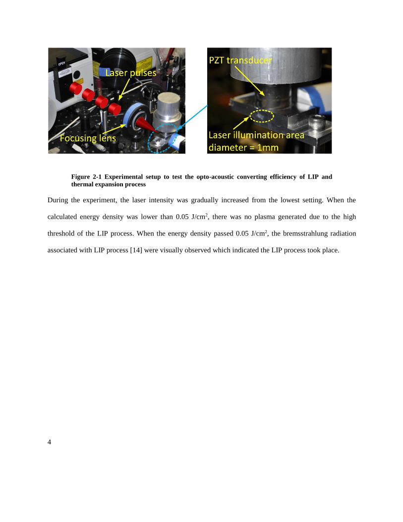
Figure 2-1 Experimental setup to test the opto-acoustic converting efficiency of LIP and
thermal expansion process
During the experiment, the laser intensity was gradually increased from the lowest setting. When the
calculated energy density was lower than 0.05 J/cm2, there was no plasma generated due to the high
threshold of the LIP process. When the energy density passed 0.05 J/cm2, the bremsstrahlung radiation
associated with LIP process [14] were visually observed which indicated the LIP process took place.
5
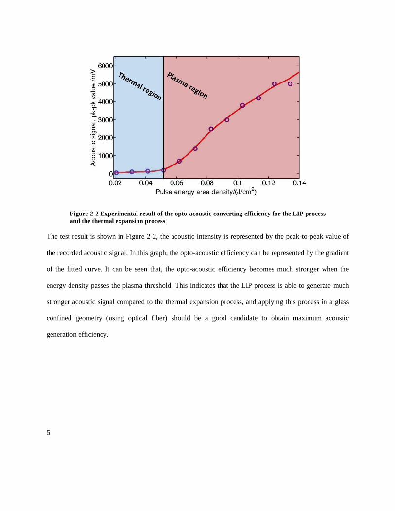
Figure 2-2 Experimental result of the opto-acoustic converting efficiency for the LIP process
and the thermal expansion process
The test result is shown in Figure 2-2, the acoustic intensity is represented by the peak-to-peak value of
the recorded acoustic signal. In this graph, the opto-acoustic efficiency can be represented by the gradient
of the fitted curve. It can be seen that, the opto-acoustic efficiency becomes much stronger when the
energy density passes the plasma threshold. This indicates that the LIP process is able to generate much
stronger acoustic signal compared to the thermal expansion process, and applying this process in a glass
confined geometry (using optical fiber) should be a good candidate to obtain maximum acoustic
generation efficiency.

6
Demonstration of single point LIP based acoustic generation and
detection
To test generating acoustic wave inside a solid with pulsed laser and optical fiber, a demonstrative LIP
acoustic generation unit was fabricated, as shown in Figure 2-3. A 105/125m step index multiple-mode
fiber was used to guide the laser. The large core in the fiber will allow higher energy transmission than
small core fibers, and the step-index structure of the fiber could also relieve the energy intensity density in
the core center thanks to the weaker self-focusing effect comparing with gradient index fibers. The
polished end of the fiber was buried in a tin pool held by a copper casting as the acoustic conductor,
allowing the usage of both PZT and FBG as the acoustic detector for characterization.
Figure 2-3. Demonstrative optical fiber LIP acoustic generating unit.
Due to the short acoustic pulse width and broad frequency range of the LIP generated acoustic wave, it is
difficult to receive an undistorted signal with a PZT. So we built an FBG based broadband acoustic
detector to evaluate the LIP generated acoustic wave. The design of the acoustic detector is shown in
Figure 2-4(a). Matching the acoustic generating unit, another copper casting with a Tin pool was used to
hold the FBG. To detect the acoustic wave propagating vertically, the FBG had to be deployed along the
cylinder. The end of the fiber was led out of the tin pool and looped to eliminate the reflection from the
7
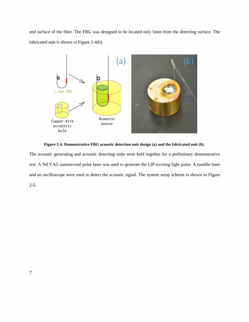
end surface of the fiber. The FBG was designed to be located only 5mm from the detecting surface. The
fabricated unit is shown in Figure 2-4(b).
Figure 2-4. Demonstrative FBG acoustic detection unit design (a) and the fabricated unit (b).
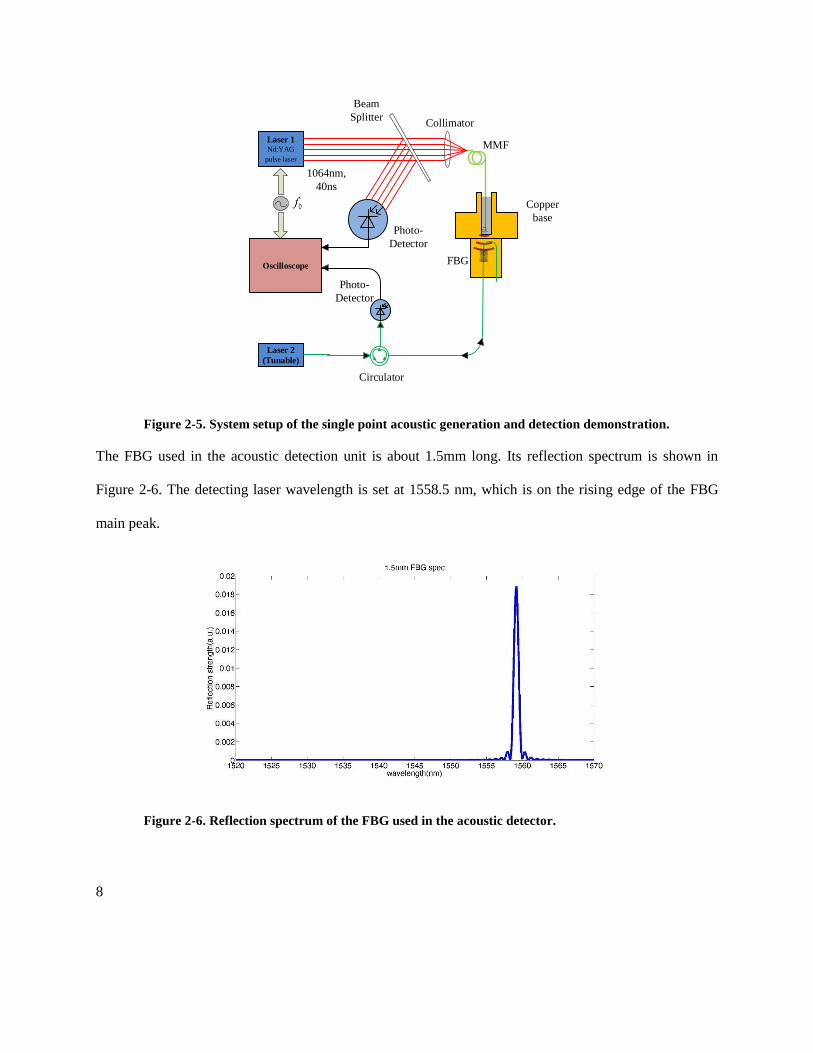
The acoustic generating and acoustic detecting units were held together for a preliminary demonstrative
test. A Nd:YAG nanosecond pulse laser was used to generate the LIP exciting light pulse. A tunable laser
and an oscilloscope were used to detect the acoustic signal. The system setup scheme is shown in Figure
2-5.
8
Laser 1Nd:YAG
pulse laser
Laser 2
(Tunable)
Oscilloscope
Photo-
Detector
Circulator
Photo-
Detector
1064nm,
40ns
Collimator
MMF
Copper
base
FBG
Beam
Splitter
Figure 2-5. System setup of the single point acoustic generation and detection demonstration.
The FBG used in the acoustic detection unit is about 1.5mm long. Its reflection spectrum is shown in
Figure 2-6. The detecting laser wavelength is set at 1558.5 nm, which is on the rising edge of the FBG
main peak.
Figure 2-6. Reflection spectrum of the FBG used in the acoustic detector.

9
The acoustic pulse width generated was calculated to be 0.16mm in space, according to the 40ns time
width of the laser pulses. As shown in Figure 2-7, the experiment result (solid line) agrees well with the
simulation result (dashed line), only with slight shape distortion and a negative tail.
Figure 2-7. Comparison of the experimental result (solid blue line) and the simulation result
(dashed red line).
To test the long distance propagation of a LIP generated acoustic wave in solid, another demonstration
was performed with a long copper rod. The experiment setup is shown in Figure 2-8.
(a) (b)
FBG
Buried fiber end
FBG
Buried fiber end40cm copper rod
Figure 2-8. Preliminary FO-SHM unit demonstration test: (a) acoustic generation and
detection units directly attached; (b) acoustic wave passes through copper rod before
detected by FBG
The acoustic signals generated by 1064nm laser pulses with 0.5mJ pulse energy are shown in Figure 2-9.
The signals have been averaged 500 times. As indicated by the signal strength in both results, the acoustic

10
vibration generated by the LIP mechanism should also be able to produce recognizable signal when
implemented on a work piece with similar dimensions.
Figure 2-9. Signals acquired with the demonstrative FO-SHM unit: (a) 1064nm laser pulse;
(b) acoustic signal acquired with FBG unit directly attached to acoustic generation unit; (c)
acoustic signal acquired with FBG unit and acoustic generation unit separated by a piece of
40cm-long copper rod
Multiplexable LIP and FBG based FO-SHM element design, fabrication
and test
As discussed in the previous section, the LIP formation breakdown can be generated in a confined
geometry to excite strong acoustic wave. To achieve the goal of multi-point sensing, a multiplexable in-
fiber acoustic excitation structure design was proposed. As shown in Figure 2-10, thin metal films are
deployed partially inside a multimode fiber, serving as the laser absorbing media which generate laser
induced plasma. The part of the laser beam that misses the metal target will redistribute in the fiber core
as it propagates, and hit the following targets.

11
Figure 2-10. Structure of multiplexing in-fiber LIP acoustic generating units.
The multimode fiber chosen for the system is 105/125μm step index fiber, due to its large core diameter
and standard cladding layer geometry. More importantly, unlike the graded-index multimode fibers which
have the GRIN lens effect [15, 16], step-index multimode fibers have no focusing effect inside the core,
which leads to a higher damage threshold than graded-index fibers with similar core diameters.
To achieve proper absorption rate on each absorber for the purpose of element multiplexing, the size of
the metal films was chosen to be 5-10μm for the 105μm core fiber. For a quasi-uniform light distribution
in the core, the calculation shows that 4.8%-9.5% of light power will be absorbed on each film. A
multiplexing of 10 units will reduce the initial light intensity to 36.7%-61.4%, which corresponds to an
acoustic intensity drop of 2.1dB-4.3dB between the first and the 10th unit.
The thickness of the metal film is another important parameter that needs optimization. A very thick
metal film will be extremely time-consuming to fabricate, and will bring challenge to the splicing of the
coated fiber. On the other hand, a very thin metal layer (nanometer scale) may degrade quickly under
strong laser pulse exposure, which will greatly reduce the element lifetime. In the tested designs,
thickness of 1-5μm was used.
The fabrication procedure of an LIP based FO-SHM element was designed as followed:
1. Cleave a 105/125µm fiber;
2. Mill a 10µm diameter, 2µm deep well on the cleaved fiber end with FIB;

12
3. Fill the well with deposited platinum with FIB;
4. Cleave another 105/125µm fiber and splice it to the treated end of the first fiber, using a standard
multimode fiber splicing technique;
5. Observe the acoustic excitation unit from the side under microscope, adjust the splicing
parameters and redo the procedure if needed;
6. Splice a 2mm long, -5dB FBG in an SMF-28e single mode fiber;
7. Attach these two fibers side by side, with an optimized distance between the two units.
A demonstrative element was fabricated, as shown in Figure 2-11.
Figure 2-11. Fabrication of a demonstrative LIP based FO-SHM element.

13
The first LIP based FO-AGU was successfully fabricated with Focused Ion Beam (FIB) and fiber splicing
techniques. A measurement with a light source and a power meter showed a 64% transmission rate of the
unit. In this section, the unit was put to the test in a simplified test bench.
A PZT detector was used to monitor the generated acoustic wave. A reference acoustic source was made
with a fiber pointing to a blade. The unit under test, the reference and the detector were all immersed in
water for convenient acoustic transmission. The setup is shown in Figure 2-12 (PZT unit not shown).
Figure 2-12. LIP unit test setup and unit breakage
When excited with laser pulses with 250uJ pulse energy, the unit broke from the splicing point (Marked
with the green circle in Figure 2-12. After the unit broke, a strong acoustic signal could still be detected
by the PZT for several pulses, and then the signal vanished. The phenomenon is believed to be a result of
the quick non-confined LIP breakdown of the metal layer remaining on the broken fiber end.

14
Both fractures of the broken LIP unit were observed under an optical microscope, as shown in Figure
2-13.
(a) (b)
Figure 2-13. Microscope images of the two fiber ends taken after the unit broke: (a) the fiber
with the well for the metal layer and (b) the mating fiber
Comparing the image of the metal-coated fiber end taken before splicing (Figure 2-14), it is obvious that
the metal film is totally blown off.
Figure 2-14. Image of the metal coated fiber end before spliced with the mating fiber

15
It is also worth noting that both fiber ends of the broken unit had smooth fracture surfaces. During the
fabrication of the first unit, relatively low arcing energy was used to avoid metal deforming. However,
according to the result, only a small part of the two fibers was spliced together, resulting in a low
mechanical strength that could not hold the structure under the force of the explosion on the metal sheet.
It indicates that stronger splicing is the key to enhancing the signal strength and extending sensor
robustness.
To obtain higher mechanical strength, the splicing conditions were adjusted in the fabrication of the
second LIP based acoustic generation unit. By applying a cleaning arc before the main arc and increasing
the main arc power, the two fiber ends were tightly bonded together, as shown in Figure 2-15. However,
after the splicing, a bubble was formed in the unit.
Figure 2-15. Improved splicing of the second LIP FO-AGU
We believe the bubble was formed by the gap in the half-filled well on the fiber tip. In the FIB machining,
the metal did not perfectly fill the well, leaving an air void when the two fiber ends met. During the arcing,
the air void expanded under high temperature and formed a bubble in the softened silica. The result of a

16
transmission test shows a transmission rate of ~10%, which is much lower than the designed value.
Comparing with the first unit, it is obvious that the bubble is the major cause of the high loss.
The unit is then tested in the same setup described in the former section. In the test, strong acoustic pulses
were generated, and no evidence of breaking was observed after multiple pulses. One of the acoustic
pulses recorded by an oscilloscope is shown in Figure 2-16.
Figure 2-16. Acoustic signal generated by the second LIP unit and detected by a PZT
detector in water
Conclusion
In this phase of the study, we have designed, fabricated and tested the LIP based acoustic generation units,
which are able to generate strong acoustic vibration. Although the performance of this LIP based FO-
AGU is promising in terms of acoustic intensity, it brings challenges in the fabrication process (time-
consuming and very costly). In addition, this structure reduces the mechanical strength of the optical fiber
so it may bring problems when attached to a sample and used in a high temperature environment.

17
3 Test and comparison of two thermal expansion based acoustic generation
schemes
Due to the problems associated with the LIP based FO-SHM design, two thermal expansion based
acoustic generation schemes were studied. They are Erbium-doped fiber (EDF) based method and
scattering-light based method. The design, test and discussion of these two routes are presented in this
section.
Erbium-doped fiber (EDF) based acoustic generation
The acoustic generation with EDF is based on the thermal expansion of the fiber. When the laser energy
is absorbed by the Er3+ ions in an EDF, part of the energy will transform into heat and cause thermal
expansion. When excited by a laser pulse, acoustic waves are generated by the instantaneous expansion
and contraction of the fiber.
Figure 3-1 Level diagram of Er3+ in EDF[17]
Among all the energy transitions of Er3+ as shown in Figure 3-1, the only one that can generate acoustic
signal efficiently is the fast non-radiative decay from the excited state to the metastable state. According
to former research [18], the lifetime of the excited state 4I11/2 is between 1~10µs, which is fast enough for
18
the acoustic generation. Another transition which can possibly generate thermal expansion is from the
metastable state to the ground state. This transition includes both spontaneous emission and non-radiative
decay, while only the latter one is related to heat generation. As reported in literature [17-20], the lifetime
of the metastable state 4I13/2 is ~10ms, which is too long for acoustic wave generation application.
In summary, the only transition we can utilize to generate acoustic wave efficiently is the non-radiative
decay from 4I11/2 to 4I13/2. Based on the 1µs~10µs timescale of this transition, it can be calculated that the
acoustic wave we could generate with EDF will have a wavelength of 1~10mm on metal.
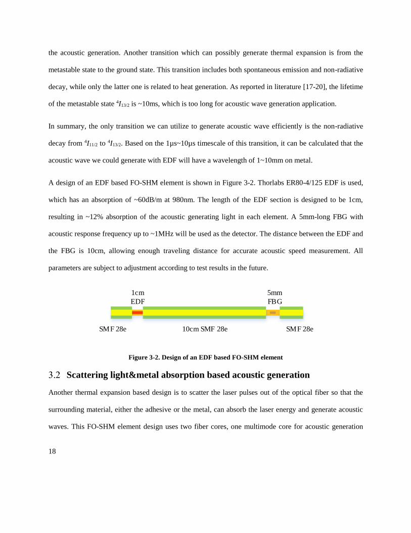
A design of an EDF based FO-SHM element is shown in Figure 3-2. Thorlabs ER80-4/125 EDF is used,
which has an absorption of ~60dB/m at 980nm. The length of the EDF section is designed to be 1cm,
resulting in ~12% absorption of the acoustic generating light in each element. A 5mm-long FBG with
acoustic response frequency up to ~1MHz will be used as the detector. The distance between the EDF and
the FBG is 10cm, allowing enough traveling distance for accurate acoustic speed measurement. All
parameters are subject to adjustment according to test results in the future.
SMF 28e 10cm SMF 28e SMF 28e
1cm
EDF
5mm
FBG
Figure 3-2. Design of an EDF based FO-SHM element
Scattering light&metal absorption based acoustic generation
Another thermal expansion based design is to scatter the laser pulses out of the optical fiber so that the
surrounding material, either the adhesive or the metal, can absorb the laser energy and generate acoustic
waves. This FO-SHM element design uses two fiber cores, one multimode core for acoustic generation

19
light propagation and the other single-mode core for probe light propagation. A femtosecond laser will be
used to inscribe scattering voids inside the large diameter core to generate scattered light which leaks out
of the core and excite acoustic wave by interacting with the surrounding material. The same femtosecond
laser will also be used to inscribe type-II FBGs for acoustic detection so the whole fabrication process can
be accomplished with one single setup. This new design eliminates the needs for fiber coating removal
and fiber splicing, hence significantly increases the mechanical strength of the fiber device and reduces
the risk of fiber breakage during embedment and fast temperature changes. Another advantage of this
design is its intrinsic high temperature compatibility. Scattering voids and type-II FBGs are created by
localized material melting and compaction associated with multi-photon ionization induced dielectric
breakdown, and which are stable up to the glass transition temperature [21]. For silica fiber, type-II FBGs
are reported to be stable during long time temperature cycling test up to 1050°C [22].
Based on the idea, three schemes were designed, from which the final design will be chosen based on the
availability of the special fiber.
a. Scheme 1
Type-II voids section
Type-II FBG
Standard step-index multimode fiber
Standard single mode fiber
Figure 3-3. Standard multimode fiber + standard single mode fiber
This option uses two separate standard fiber and bond them together with a high temperature coating. A
standard multimode fiber is inscribed with scattering voids and used as the acoustic generation unit. The
FBG is inscribed in a standard single mode fiber and used as the acoustic detection unit. The advantage is
that the acoustic generation light and probe light are completely isolated so there will not be any

20
unwanted interference. The drawbacks are the increased overall size and the complexity in fiber
embedment.
b. Scheme 2
Type-II voids section
Type-II FBGDouble cladding fiber
Figure 3-4. Un-doped double cladding fiber (DCF)
This option uses a double cladding fiber with undoped core and silica outer cladding. The acoustic
generation light propagates inside the inner cladding and core, while the scattering voids are inscribed in
the inner cladding only so it doesn’t introduce additional loss to the probe light which propagates inside
the single mode core. The FBG is inscribed inside the core with tight focus laser beam (spot size < 1um)
so it generates a minimum loss to the acoustic generation light. This type of fiber needs custom
fabrication, and can be pursued in the next phase of this project.
c. Scheme 3
Type-II voids section
Type-II FBGTwin core fiber
Figure 3-5. Twin-core fiber
This option is similar to option 1 but uses a twin core fiber, a type of special fiber with two cores and one
cladding. This type of fiber needs custom fabrication, and can be pursued in the next phase of this project.

21
Experimental comparison
In this section, we built experimental setups to compare the acoustic generation capabilities of the
proposed thermal expansion based acoustic generation methods. The system schematic is shown in Figure
3-6. A 980nm pulsed laser with 2W peak power was used as the acoustic excitation source and modulated
by a function generator to output burst pulses with 1KHz burst rate and 90~200KHz pulse frequency. 10%
of the total power was split and monitored by a photodetector, while the remaining power went into the
acoustic generation unit (AGU), which in this experiment is a segment of single mode fiber with
scattering voids or EDF. The AGU was buried inside a metal piece and a PZT was attached to monitor the
generated acoustic signal. The PZT signal was then amplified by a band pass amplifier and averaged to
show the acoustic signal on an oscilloscope. The light through the AGU was monitored by another
photodetector as a reference on how much energy is absorbed by the AGU.
Photodetector980nm
pulsed laserOscilloscope
coupler
Function
generator
980nm
isolator
90%
10%
20 dB
attenuator
Band pass
amplifier
PZT
Metal piece
AGU
Figure 3-6. AGU test scheme with a PZT as the acoustic detector
The key components used in the experimental setup are listed as follows.

22
Table 1 Equipment used for thermal expansion based acoustic generation methods
comparison
980nm pulsed laser ALPhANOV PDM 980
C-band tunable laser Newport TLB-6700
Oscilloscope Lecroy 725Zi
Photodetector Menlosystem FPD510
Balanced photodetector Newport 2117-FC
Bandpass amplifier Preamble 1822
Function generator Tektronix AFG 3252
Pictures of the completed experimental setup are shown in Figure 3-7.
(a) (b)
Figure 3-7. Experimental setup of the EDF based FO-SHM system: (a) acoustic generation
system using a 980nm pulsed laser; (b) test bench
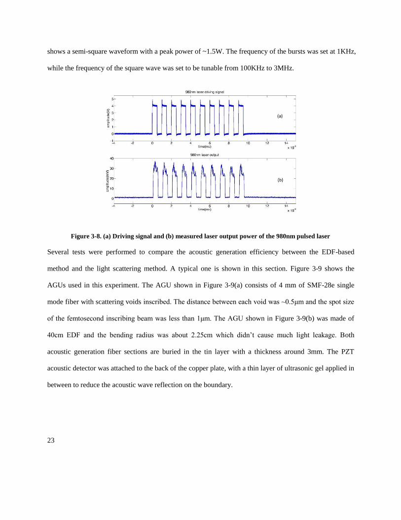
To acquire high-power light pulses with specific pulse width, a burst square wave train was generated by
a function generator as the controlling signal. As shown in Figure 3-8 (b), a laser power measurement
23
shows a semi-square waveform with a peak power of ~1.5W. The frequency of the bursts was set at 1KHz,
while the frequency of the square wave was set to be tunable from 100KHz to 3MHz.
Figure 3-8. (a) Driving signal and (b) measured laser output power of the 980nm pulsed laser
Several tests were performed to compare the acoustic generation efficiency between the EDF-based
method and the light scattering method. A typical one is shown in this section. Figure 3-9 shows the
AGUs used in this experiment. The AGU shown in Figure 3-9(a) consists of 4 mm of SMF-28e single
mode fiber with scattering voids inscribed. The distance between each void was ~0.5μm and the spot size
of the femtosecond inscribing beam was less than 1μm. The AGU shown in Figure 3-9(b) was made of
40cm EDF and the bending radius was about 2.25cm which didn’t cause much light leakage. Both
acoustic generation fiber sections are buried in the tin layer with a thickness around 3mm. The PZT
acoustic detector was attached to the back of the copper plate, with a thin layer of ultrasonic gel applied in
between to reduce the acoustic wave reflection on the boundary.

24
Figure 3-9. (a) AGU made with 4mm section of SMF-28e with scattering voids inscribed by a
femtosecond laser; (b) AGU made with 40cm coiled EDF (Thorlabs ER80-8/125)
The photodetector monitoring results showed that the transmission loss for the scattering-based and EDF-
based AGUs are 1.25dB and 6dB respectively, corresponding to absorption ratio of 25% and 75%. The
acoustic signals generated by these two AGUs with the same 980nm laser pulses are shown in Figure
3-10. The repetition rate of the 980nm laser pulses was set to 90KHz.
Figure 3-10. Acoustic signals generated by the scattering-based and EDF-based AGUs

25
The results clearly show that generating acoustic vibration with scattered light is superior in terms of
opto-acoustic conversion coefficient compared to the EDF-based mechanism. The significant difference
in the acoustic generation efficiency between the two methods is discussed in the following section.
Analysis of opto-acoustic conversion efficiency
Let’s consider an acoustic generation unit with cylindrical geometry and cross section diameter DM. When
it absorbs energy from a laser pulse, the material temperature arises. The temperature increment is:
where P is the pulse peak power, 0t is the duration of the pulse, is absorption rate, CV is the specific
heat of the material, m is the mass of the unit and L is the length of the unit.
The corresponding strain is
Here is the density of the material and is the linear thermal expansion coefficient.
The generated acoustic pressure is approximated by the tensile stress caused by this strain.
0
V
QT
m C
Q P t
(1)
2
Mm L D
(2)
0
2
M V
P tT
L D C
(3)
T (4)

26
While the parameter 0
2
M
P tA
L D
is independent of the properties of the material, the acoustic
pressure strength is mainly decided by four intrinsic coefficients of the material (Young’s modulus,
thermal expansion coefficient, density and specific heat). Comparing these properties of fused silica and
tin as shown in Table 2, we can see that the acoustic strength will be about 65 times stronger if we switch
the acoustic generating material from fused silica to tin.
Table 2. Material properties
Fused silica Metal tin
E 73 GPa 87 GPa
0.55 ppm/K 23.4 ppm/K
2.648 g/cm3 7.28 g/cm3
VC
740
1 1J kg K
210
1 1J kg K
V
E
C
22.05 10 1.33
0
2
0
2
M V
V M V
P tp E T E
D C L
P tE EA
C L D C
(5)

27
Since the fiber core is made of Erbium doped fused silica, this analysis suggests that directly illuminating
metal with excitation light will generate a significantly stronger acoustic signal as compared to the EDF-
based method.
Conclusion
Based on the analysis, the scattering based thermal expansion process was chosen as the acoustic
generation mechanism in the FO-SHM element. The AGU designed based on this mechanism showed
sufficient opto-acoustic generation efficiency and is mechanically strong. Due to the limitation of
available optical fiber, we chose to use the two optical fiber scheme to build the FO-SHM element. This
means that each FO-SHM monitoring elements will be formed with two fiber, one multimode fiber for
acoustic excitation laser transmission, another single-mode fiber for the probe light transmission.
Microstructures will be fabricated inside the multimode fiber for light scattering, and the FBG will be
fabricated in the single mode fiber for acoustic detection. The acoustic wave will be generated from the
surrounding adhesive by its absorption of the laser energy. The details of the FO-SHM design and the
overall system design are presented in the following sections.

28
4 Simulations of the ultrasonic pulse based multi-parameter monitoring
scheme
FEM simulation of crack and corrosion detection using the elastic wave
model
In this section, we present the modeling of crack and corrosion detection based on linear elastodynamic
wave propagation in uniform and isotropic material. Linear elastodynamic wave theory describes the
propagation of elastic waves inside linear solid materials. Among all the parameters associated with an
elastic wave, time variant strain is what we could detect experimentally in the crack and corrosion
detection. The governing equations are shown as follows (in direct tensor form)[23]:
Here σ is the Cauchy stress tensor, ε is the infinitesimal strain tensor, u is the displacement vector, C is
the fourth-order stiffness tensor, F is the body force per unit volume, and ρ is the mass density of the
material.
By solving these equations with a finite element method, the time variant strain at any given point in the
material can be given as:
Equation of motion: ..
· σ F u (6)
Strain-displacement equations: 12
( )T ε u u (7)
Constitutive equations: :σ εC (8)

29
In a 2D simulation, if the FBG is placed along the x direction, the parameter of interest will be xx since it
is the only strain component that can be detected by the FBG.
In the elastic wave model, multiple propagation modes are supported due to the existence of shear stress.
The bulk waves which propagate inside the material include both a pressure wave (P-wave) and a shear
wave (S-wave). They have different propagation speeds and are non-dispersive in uniform, isotropic
media. However, the speed of P-wave and S-wave are both dependents of temperature. This property
could be used for temperature compensation in a multi-parameter measurement system.
Besides bulk waves, the surface wave is also important for traditional ultrasonic NDE method. Generally,
the surface wave is the superposition of P-wave and S-wave which follows the surface curvature in
propagation and decays rapidly with increased depth. The surface wave could propagate over longer
distance than bulk wave and has relatively high amplitude, so it is often used to monitor discontinuities on
and near the surface.
There are also guided waves which depend specifically on the medium geometry. Take a plate waveguide
for example, if the thickness of the plate is less than 3-4 times of the acoustic wavelength, bulk waves will
not be supported and guided waves (or Lamb waves) will take place.
Another important concept in the elastic wave propagation model is the mode conversion. When certain
modes of elastic wave encounter a medium interface, mode conversion will happen and multiple modes
1 1
2 2
1 1
2 2
1 1
2 2
yx x x z
xx xy xz
y y yx zyx yy yz
zx zy zz
yxz z z
uu u u u
x y x z x
u u uu u
x y y z y
uuu u u
x z y z z
(9)[23]

30
will be generated at different angles with different amplitudes, which could greatly increase the
demodulation complexity.
4.1.1 Simulation model building in COMSOL
To build the simulation model, optimization of the parameters, including the minimum size of detectable
crack and acoustic pulse duration, has been conducted.
The crack formation and propagation was intensely studied in the research field of mechanical structures.
According to former reports, cracks start with a small initial size and then grow into larger critical size
[24, 25]. The initial size of cracks is generally described by a lognormal distribution, with the mean value
and standard deviation of (0.526mm, 0.504mm) [25]. On the other hand, the size of critical cracks highly
depends on the geometry of the structure. For the current simulation, a crack size reasonably larger than
the initial crack size was chosen.
As for the acoustic pulse duration, shorter acoustic wavelength will suffer from stronger attenuation in
material while longer wavelength has lower sensitivity to small features in the material. It is reported that
the attenuation of acoustic waves increases severely above 10MHz for steel structures [26, 27]. As a
general rule of thumb in ultrasound NDE, the probe acoustic wavelength should be shorter than 2/3 of the
flaw size to have a reasonable chance of successful detection. Besides, in our laser acoustic generation
scheme, using shorter laser pulse will allow us to acquire higher optical-acoustic conversion efficiency
despite the generation mechanism deployed.
Considering all these factors, the cracks were modeled as 5mm*0.1mm air voids inside iron specimens,
and the excited acoustic pulses were simulated as Gaussian pulses with 500ns FWHM (~3mm wavelength
for P-wave, ~2mm wavelength for S-wave). Other parameters in the simulation are shown as follows:

31
Table 3 Simulation model properties
Specimen 300mm*100mm rectangular iron
Acoustic excitation area 125µm*1mm rectangular silica
Corrosion thickness 5mm
Distance between acoustic generator and detector 100mm
Fiber attachment 2mm under surface
Crack position center of specimen
The geometry of the simulation setup is shown in Figure 4-1.
Acoustic excitation area
Acoustic detection fiber
Crack
Corrosion surface
10cm
30cm
Figure 4-1. Simulation specimen geometry.
4.1.2 Simulation result
In this preliminary simulation, elastic wave propagation modes are studied and the time variant strain
component at the detecting fiber-optic sensor was recorded under different conditions for comparison.
Figure 4-2 shows the elastic wave trace in the specimen. The length of the acoustic pulse is set to be 5mm
to suppress multiple reflection near the acoustic source for better visualization. In Figure 4-2(a), P-wave,

32
S-wave, surface wave and crack reflection wave could be clearly observed. The propagation speed of P-
wave and S-wave calculated were around 5700m/s and 3100m/s respectively, which agrees well with
theoretical values (5770.8m/s and 3138.5m/s). Surface wave speed was calculated to be around 2700m/s,
which is slightly slower than S-wave speed as predicted by the elastic wave theory. As the P-wave hits the
bottom surface, two reflection waves with different speed were generated from due to mode conversion,
which are the faster P-wave and the slower S-wave, as shown in Figure 4-2(b).
S-wave
Surface wave
Crack signal wave P-wave
P-wave
Reflection generated S-wave
Reflection generated P-wave
(a) Time=20µs
(b) Time=30µs
Figure 4-2. Simulation results of elastic wave propagation trace in a specimen with a crack.
The signals induced by the crack were simulated with a 2.5mm acoustic probe pulse, as shown in Figure
4-3. The crack-induced signals were marked in the figures, which could be easily recognized.

33
Figure 4-3. Simulation results of crack-induced acoustic signals.
The strain signals in a corroded specimen are also simulated with 2.5mm acoustic pulses. To amplify the
signal change induced by the corrosion, a relatively big corrosion depth of 5mm was simulated on the
bottom surface. The comparison data is presented in Figure 4-4.

34
Figure 4-4. Simulation results of corrosion-induced acoustic signals.
The black vertical line in Figure 4-4 marks the boundary between the direct P-wave and echo signals from
the bottom surface. Since the direct P-wave should not be affected by the corrosion, the shift observed in
the corroded data was attributed to the computational error of the software under different meshing
conditions. The phenomenon also presents in the crack simulation data (Figure 4-3).
From this set of simulations, it can be seen that the ultrasonic pulse method can be used to monitor the
thickness change and appearance of cracks by the observation of peak shifts and new peak appearances. It
is also possible to monitor the temperature change with this method because the thickness change doesn’t
affect the direct pressure wave. So the location of this peak in the time domain is solely determined by the
temperature dependent material properties. The following section shows a calculation of the temperature
induced pressure wave velocity change and the corresponding peak delay with a reasonable distance
between the acoustic generation/detection pair.

35
Temperature induced acoustic velocity change calculation
As indicated in the previous section, the acoustic velocity of the direct pressure wave can be used to
monitor the sample temperature. By setting an appropriate gap between the between the acoustic
generation unit and the FBG, acoustic velocity can be directly measured by the fly time of the first peak in
the AE. The velocity of the longitudinal wave in solids is described as:
where B is the bulk modulus, is the shear modulus, E is the Young’s modulus, is the Poisson’s ratio
and is the density if the material. While the theoretical temperature dependence of these elastic
constants varies on different materials, some empirical equations can be used on steel to get an estimation
of the relationship between fly time variances and temperature changes. These equations are suggested by
two scientific organizations (D.T.U. and Eurocode) and adopted in most works that approach the thermal-
mechanical analysis of steel structures [28, 29].
For Young’s modulus:
For Poisson’s ratio:
3 4 (1 )
3 (1 2 )(1 )
B Ev
(10)
( ) 11 , 20 600
(20)2000ln( )
1100
( ) 690 0.69, 600 1000
(20) 53.5
E tfor C t C
tE
E t tfor C t C
E t
(11)

36
Since the density variance is negligible, the ratio ( )
(20)
v t
v can be calculated as shown in Figure 4-5 (a).
(a) (b)
Figure 4-5. (a) The ratio of the sound velocity at temperatures from 0-1000°C to the sound
velocity at 20°C; (b) the ratio of the fly time variance at temperatures from 0-1000°C to the
acoustic wave propagating distance
Since Eq. 11 is not an accurate description of the sound speed when temperature approaches the melting
point, we only consider situations below 450°C to get an estimation of fly time delay. Using the
longitudinal wave speed in iron at room temperature (v(20)=5130m/s), the ratio of fly time variance over
temperature difference and distance between the voids and the FBG is presented in Figure 4-5(b). The
lowest response rate appears at the low temperature end and the value is about 0.1ns/(cm·°C). It means
that with 1cm distance between voids and FBG, the signal acquiring and analysis process will need to
have a temporal resolution higher than 1ns to obtain a 10°C temperature resolution. Thus, 1cm was set as
the starting point in the future temperature monitoring experiments.
5
5
( ) 3.78 10 0.283 , 0 450
( ) 9.20 10 0.259 , 450
t t for t C
t t for t C
(12)

37
Simulation of fiber Bragg grating (FBG) response to short acoustic pulse
In conventional FBG acoustic detection methods, it is assumed that the width of the acoustic pulses is
much longer than the physical length of the detecting FBG. Under this assumption, the strain exerted on
the FBG can be approximated to be uniform at any given time. Therefore, the shape of the acoustic pulse
can be easily reconstructed from the intensity change of the reflected light, as shown in Figure 4-6.
Figure 4-6. While a slow acoustic pulse (a) passes through an FBG, the instantaneous stress
will be indicated by a shift in its reflection spectrum (b). The reflection intensity of a laser
with its wavelength fixed on one edge of the main peak will be modulated in response to the
stress wave (c).
However, this assumption is not applicable in our acoustic defect detection scheme. To detect a defect in
metal, the equivalent wavelength of the acoustic wave must be shorter than the dimension of the defect.
Since the size of the defects in metal could be as small as several millimeters, the effective wavelength of
the acoustic pulse has to be at the sub-millimeter level, which is even shorter than the length of most
FBGs. Thus it is necessary to analyze the temporal response of an FBG to a relatively short acoustic pulse
in order to understand the recorded AE in the following experiments.

38
4.3.1 The transfer matrix method
In this section, the coupled-mode theory and the transfer-matrix method are used to simulate the reflection
spectrum of an FBG.
In the coupled-mode theory, the electric field is written as a superposition of the forward and backward
propagating modes:
where satisfies the scalar wave equation for an unperturbed fiber:
where /k c is the wavenumber in vacuum and effn k is the scalar propagation constant.
Assuming the FBG refractive index perturbation has the following periodic form:
where acn is the amplitude of the refractive index change, and is the period of the FBG.
The forward propagating component t(z) and backward propagating component r(z) follow the coupled-
mode equations:
1 1( , , ) ( ) ( , , ) ( ) ( , , )E x y z b z x y z b z x y z
(13)[30]
2 2 2 2
2 2 2 2 2
{ ( , ) } 0
/ /
t
t
k n x y
x y
(14)[30]
2 2 2
( )cos( ( ))acn n n z z z
(15)[30]

39
where / ,
( )( ) acn z
q z
and arg( ( )) ( )
2q z z
.
The coupled-mode equations shown in Eq. 16 can be written in transfer matrix form as[30]:
By dividing the FBG into small sections and multiply all the transfer matrix of each section, the
relationship between the electric field at position L and at position 0 on the fiber can be written as:
where the matrix T stands for the chain multiplication of the transfer matrices of each section. The relative
values of t(L), r(L) and r(0) are calculated by defining t(0) to be 1. When using a weak FBG, the relative
propagating wave intensity t(L) is approximately 1, so the back reflected intensity r(0) can be calculated
as:
( )
( )
dti t q z r
dz
dri t q z r
dz
(16)[30]
cosh( ) sinh( ) sinh( )( ) ( )
( ) ( )sinh( ) cosh( ) sinh( )
qz i z z
t z z t z
r z z r zqz z i z
(17)[30]
11 12
21 22
( ) (0)
( ) (0)
T Tt L tT T
r L r T T
(18)[30]
21 22(0) /r T T
(19)[30]

40
4.3.2 Simulation result
A 32ns Gaussian acoustic pulse was used in the simulation, which is chosen according to the pulse width
of the pump laser currently used in the system. The length of the detecting FBG was set to 1.5mm. The
acoustic detection was conducted by using a laser with a wavelength at the rising edge of the FBG main
reflection peak. When the short acoustic pulse passed the FBG, the period of the FBG was partially
modulated, and the instantaneous reflection intensity could be calculated at any given time. The
calculated reflection intensity signal is shown in Figure 4-7.
Figure 4-7. The reflection response of a 1.5mm long FBG to a 32ns (0.16mm long in space)
acoustic pulse. Red line: acoustic pulse. Blue line: simulated FBG response signal.
As shown in the simulation result, the response signal has a length of ~220ns in time, and ~1.1mm in
space correspondingly. The result can be understood as that the pulse width of the recorded acoustic pulse
is approximately equal to the sum of the original pulse width and the acoustic wave travel time on the
FBG. This means using a shorter FBG can improve the spatial resolution of the detector, as long as the
acoustic pulse is shorter than the FBG.

41
5 The design and demonstration of an all fiber optic structural health
monitoring system
According to the information acquired in the previous sections, a detailed overall system design is
presented here.
System design and operation procedure
Figure 5-1 (a) System schematic of an FO-SHM system; (b) Sample spectrum of an FO-SHM
system containing 5 nodes
The schematic of a multiplexed FO-SHM system is shown in Figure 5-1(a). The acoustic detection fiber
used was a Corning SMF-28e standard fiber, and the acoustic excitation fiber was a 105/125 μm step-
index multimode fiber. The laser used for acoustic excitation was a flash lamp pumped 1064nm Nd:YAG
free space laser with 10 Hz repetition rate and 50ns pulse width. The laser pulse energy was 150uJ. An
optical sensing interrogator was used for fast spectrum acquisition, and for monitoring the spectra of all
FBGs in the sensing chain as shown in Figure 5-1(b). After obtaining the system spectrum, the spectrum
location of the target FBG in the current cycle can be read. A C-band tunable laser was used as the probe
light, the wavelength of which was tuned to the FWHM wavelength of the target FBG. A balanced
photodetector was used to measure the fluctuation of the reflected optical power from the target FBG,
which is related to the acoustic signal strength. A 50:50 fiber coupler was employed before the photo-
detector to provide a reference arm, which eliminated the DC component in the measurement and allowed

42
the detector to work at the highest possible gain. A high-speed oscilloscope with 2 GHz bandwidth was
used to record the acoustic signal detected by the photo-detector. The system was switched between the
FBG spectrum acquisition cycle and the acoustic signal acquisition cycle by a MEMS optical switch. The
parameters of our interest can be monitored by the analysis of the obtained spectrum information and the
acoustic signature. All the instruments in the system were controlled and synchronized by a PC through
USB and Ethernet ports.
Experimental setup
We used a free space Nd:YAG pulsed laser for the acoustic excitation due to its high energy/pulse
capability. During the previous research phases where the experiment was only preliminary or
confirmatory, a simple free space to fiber coupling setup was used. Basically, we used a long focal length
lens to focus the pulsed laser into the multimode fiber. This setup showed problems like unstable coupling
efficiency, difficulties in the alignment and damages to the fiber core during the alignment process. To
solve this problem and reduce the alignment time for an everyday experiment, we designed and built the
following coupling system.

43
10
64
no
tch
fi
lter
CCD
1064 filter
40dB ND filter
532nm LED lamp
PBS N-PBS
ND filters
Tube lens
Fiber collimator
Condenser
Target multimode
fiber
Illumination and CCD imaging part
Iris Objective lensIris
Laser power monitoring and trigger providing part
Laser coupling part
Figure 5-2 Simplified pulse laser optical fiber coupling scheme with CCD imaging system
Figure 5-2 shows a simplified schematic of the pulse laser to optical fiber coupling scheme This system is
composed of a CCD imaging module, an illumination module and a laser power monitoring module. The
imaging module provides the real-time image of the fiber coupling end surface and aids the alignment of
the fiber core to the laser beam. The alignment procedures are as indicated in Figure 5-3(b). The fiber
core is firstly moved far away from the laser beam and a single laser pulse is used to put a damage mark
on the surrounding ferrule. Then a software provided cross hair is aligned with the damage mark to
indicate the laser beam location. Finally, the core is aligned with the cross hair and the laser will be put to
continuous working mode. The laser power monitoring module is connected to a photodetector by a
single mode fiber. Besides monitoring the laser pulse intensity, it also provides a trigger signal for the
sensing system. The completed coupling system is shown in Figure 5-3(a).

44
Figure 5-3 (a)Free-space laser to optical fiber coupling system; (b)Fiber core alignment
method
Figure 5-4 shows the preliminary experiment setup we used to demonstrate the feasibility of the
multiplexed FO-SHM system. Despite the large size of the current system setup, it is possible to replace
most of the equipment with smaller size substitutes and build the overall system in a portable enclosure.
Figure 5-4 Preliminary experiment setup

45
FO-SHM node installation and acoustic signature analysis
To demonstrate the multi-parameter monitoring capability of this FO-SHM system, a quarter-inch thick
7075 aluminum plate was used as the device under test (DUT). A single FO-SHM node was surface-
attached to the aluminum plate as shown in Figure 5-5 (a). The FBG section was attached by an epoxy
while the acoustic generation unit was attached with an epoxy-graphite mixture. The cured epoxy was
semi-transparent and the added graphite helped increase laser absorption. The microstructure used in this
acoustic generation unit was a special splicing point fabricated with a thermal fusion splicer as shown in
Figure 5-5 (b). This structure can be easily fabricated by moving the two fiber ends to different heights
while applying arc to splice them, and the light scattering ratio can be controlled by using different offset
height. The light scattering ratio on this node was 40%.
To find the optimized location to mount the FO-SHM unit on the DUT, two sets of pre-installation tests
were performed. In the first set of the pre-installation tests, an extrinsic fabry-perot interferometric (EFPI)
fiber sensor and direct laser illumination were used to generate and record the acoustic signal. Figure 5-5
(c) shows the schematic for this test. A multimode fiber transmitting the excitation laser pulses was
positioned to directly illuminate the surface of the DUT and generate pulsed acoustic vibrations. The
polished end of a single-mode fiber was placed near the reflective surface of the DUT, forming a Fabry-
Perot interferometer (FPI) that monitors the normal displacement of the surface. With this setup, we were
able to monitor the acoustic signature of the DUT while changing the locations of the acoustic excitation
and detection. In these tests, the acoustic generation point and the acoustic detection point were placed
about 20 mm to the nearest edge of the DUT, and the distance between themselves (source-receiver
distance) was linearly increased. In the second test set, the FPI in the first test set was replaced with a
surface attached FBG. The distance to the nearest edge was also 20 mm.
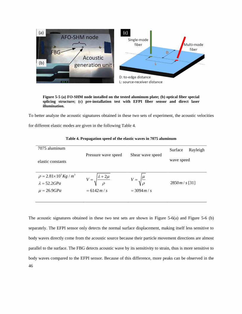
46
Figure 5-5 (a) FO-SHM node installed on the tested aluminum plate; (b) optical fiber special
splicing structure; (c) pre-installation test with EFPI fiber sensor and direct laser
illumination.
To better analyze the acoustic signatures obtained in these two sets of experiment, the acoustic velocities
for different elastic modes are given in the following Table 4.
Table 4. Propagation speed of the elastic waves in 7075 aluminum
7075 aluminum
elastic constants
Pressure wave speed Shear wave speed
Surface Rayleigh
wave speed
3 32.81 10 /
52.2
26.9
Kg m
GPa
GPa
2
6142 /
V
m s
3094 /
V
m s
2850 /m s [31]
The acoustic signatures obtained in these two test sets are shown in Figure 5-6(a) and Figure 5-6 (b)
separately. The EFPI sensor only detects the normal surface displacement, making itself less sensitive to
body waves directly come from the acoustic source because their particle movement directions are almost
parallel to the surface. The FBG detects acoustic wave by its sensitivity to strain, thus is more sensitive to
body waves compared to the EFPI sensor. Because of this difference, more peaks can be observed in the

47
second set of acoustic signatures. In Figure 5-6 (a) and (b), three distinguishable peaks are found in the
acoustic signatures. The locations of these peaks in the time domain are recorded by a peak finding
algorithm and used in the following curve fitting formula (Eq. 20) to determine their propagation
velocities and numbers of reflection experienced.
In this equation, t is the peak location in time domain, L is the source-receiver distance, D is the distance
from the source-receiver line to the presumed reflection surface, V is the velocity of a certain elastic mode,
and is a needed term mainly to compensate two possible errors: 1) the error in the recorded source-
receiver distance; 2) the difference between the peak location in time domain and the actual travel time of
the wavefront of a certain acoustic pulse.
Table 5. Curve fitting results of the three peaks and the expected values
Curve fitting result Expected value
( / )V m s ( )D mm ( )mm ( / )V m s a ( )D mm b
Direct R-wave 2894.7 0 1.33 2850 0
Reflected R-wave 2824.1 19.4 0.88 2850 20
Direct P-wave 6110.4 0 2.10 6142 0
aData refer to Tab. 1; bData from the actual experiment setup.
2 2(2 ) ( )D L
Vt
(20)

48
The results of the curve fitting are shown in Figure 5-6. By comparing the curve fitting results to the
expected values, these three peaks are identified to be the directly propagating surface Rayleigh wave
(referred to as direct R-wave), the side reflected surface Rayleigh wave (referred to as reflected R-wave),
the directly propagating pressure wave (referred to as direct P-wave). An “In-direct wave zone” is marked
in Figure 5-6 (a) because it is after the slowest direct wave (direct R-wave). Inside this zone, the area
before the fastest possible side reflection wave (side reflected pressure wave) is marked as the “Bottom
reflection zone” in Figure 5-6 (b).
Figure 5-6 (a) Acoustic signatures obtained with EFPI sensor and direct laser surface
illumination, the shift of each curve represents the source-receiver distance; (b) Acoustic
signatures obtained with FBG sensor and direct laser surface illumination, the shift of each
curve represents the source-receiver distance; (c) The final acoustic signature of the FO-
SHM unit and its related acoustic signatures from the two pre-installation tests.
Based on the findings in the pre-installation tests, the final orientation of the FO-SHM unit on the DUT
was set to be 20.5 mm away from the nearest edge and the source-receiver distance was chosen to be 7
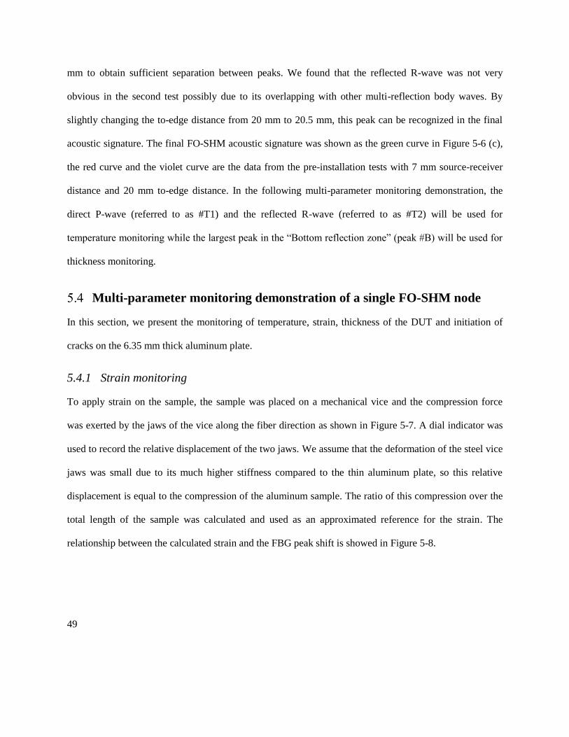
49
mm to obtain sufficient separation between peaks. We found that the reflected R-wave was not very
obvious in the second test possibly due to its overlapping with other multi-reflection body waves. By
slightly changing the to-edge distance from 20 mm to 20.5 mm, this peak can be recognized in the final
acoustic signature. The final FO-SHM acoustic signature was shown as the green curve in Figure 5-6 (c),
the red curve and the violet curve are the data from the pre-installation tests with 7 mm source-receiver
distance and 20 mm to-edge distance. In the following multi-parameter monitoring demonstration, the
direct P-wave (referred to as #T1) and the reflected R-wave (referred to as #T2) will be used for
temperature monitoring while the largest peak in the “Bottom reflection zone” (peak #B) will be used for
thickness monitoring.
Multi-parameter monitoring demonstration of a single FO-SHM node
In this section, we present the monitoring of temperature, strain, thickness of the DUT and initiation of
cracks on the 6.35 mm thick aluminum plate.
5.4.1 Strain monitoring
To apply strain on the sample, the sample was placed on a mechanical vice and the compression force
was exerted by the jaws of the vice along the fiber direction as shown in Figure 5-7. A dial indicator was
used to record the relative displacement of the two jaws. We assume that the deformation of the steel vice
jaws was small due to its much higher stiffness compared to the thin aluminum plate, so this relative
displacement is equal to the compression of the aluminum sample. The ratio of this compression over the
total length of the sample was calculated and used as an approximated reference for the strain. The
relationship between the calculated strain and the FBG peak shift is showed in Figure 5-8.

50
Figure 5-7 Strain test setup
Figure 5-8 (a) FBG spectrum monitoring during the strain change process; (b) FBG peak
location shifts caused by the strain changes.
A linear curve fitting of the FBG peak location data gives a strain sensitivity at 0.101 nm/millistrain. The
following Eq. (21) shows the theoretical relationship between the FBG peak location shift and the applied
strain along the fiber axis[32]. B
is the FBG peak wavelength which is around 1560 nm in our
experiment, n is the effective refractive index of the optical fiber which is about 1.4682 at 1550nm for the
Corning SMF-28e we used, is the Poisson’s ratio which is 0.17 for silica, p11 and p12 are the
components in the strain-optic tensor which are 0.1 and 0.285 respectively for silica[33].

51
This calculation yields a theoretical strain sensitivity of about 1.2 nm/millistrain. The difference between
this theoretical value and the linear curve fitting result can be used to calculate the strain transfer ratio
from the host material to the FBG, which is around 0.101/1.2=8.4%. In the prior research[34], the strain
transfer ratio was found to be increasing with the increase of the adhesive length and to ranging from 56%
to 82% for adhesive length from 5 cm to 15 cm. Considering that the adhesive length is only 3.5 mm in
our experiment, we believe 8.4% strain transfer ratio is reasonable.
5.4.2 Thickness monitoring
During the thickness monitoring demonstration, the sample was milled off by about 10% of the initial
thickness from the bottom by 4 incremental steps. The machining process is illustrated in Figure 5-9.
Figure 5-9 Milling off sample bottom to simulate the corrosion
The acoustic signatures obtained at these thicknesses are shown in Figure 5-10. We can see that the
temperature indication peak #T1 and #T2 did not shift during the thickness changing process. This is
2
12 12 111 [ ( )]
2
B
B
np p p
(21)

52
because that these two peaks are acoustic waves traveling along the surface and have no interaction with
the bottom of the sample. The thickness indication peak #B, shifted almost linearly during the thickness
changes. The total travel length for peak #B can be calculated by 2 2
( (2 ) )L N t , where L is the source-
receiver distance, t is the thickness of the sample and N is an integer representing how many rounds the
wave gets reflected before it reaches the receiver. When the relative change of the thickness is small, the
travel length difference may be approximately governed by Eq. (22), which explains the linear
relationship between the peak shift and the thickness change.
(3)
Figure 5-10 (a) Acoustic signatures in the thickness monitoring test; (b) peak #T1 center
shift; (c) peak #B center shift; (d) peak #T2 center shift.
5.4.3 Temperature monitoring
In the temperature monitoring demonstration, the sample was placed inside a temperature control furnace
while the temperature was raised step by step and was stabilized for about 1 hour at each step before a
2 2 2 2 1/ 2
( (2 ) ) 2 ( (2 ) )L N t N L N t t
(22)

53
measurement was taken. Figure 5-11 shows the time domain shifts of the three signature peaks due to the
temperature induced acoustic velocity changes. The linear curve fittings give the peak shift versus
temperature response rates for these monitored peaks. Using these rates and the temporal locations of
these peaks, the acoustic velocity change rates can also be calculated. The results are presented in Table 6.
Table 6. Peak location associated response rates to temperature change
Peak #T1 #B #T2
Peak shift over temperature (ns/oC) 2.26 3.52 5.34
Acoustic velocity change percentage over
temperature (10-3 /oC)
1.31 0.63 0.36
Figure 5-11 (a) Acoustic signatures in the temperature monitoring test; (b) peak #T1 center
shift; (c) peak #B center shift; (d) peak #T2 center shift.
The FBG spectra were also recorded during the temperature changing process and are shown in Figure
5-12 (a). The FBG peak locations are shown in Figure 5-12 (b) and a linear curve fitting shows that its
response rate to temperature change is about 13.4 pm/oC in this temperature range.

54
Figure 5-12 (a) FBG spectrum monitoring during the temperature change process; (b) FBG
peak location shifts caused by the temperature changes.
5.4.4 Crack detection
To demonstrate the capability of the system to actively detect a crack, a slot with about 1 mm width, 3
mm depth, and 1cm length was machined on the sample 1cm away from the FO-SHM node as shown in
Figure 5-13 (a). The acoustic signature evolution is shown in Figure 5-13 (b). Comparing the acoustic
signature with/without the crack, it can be seen that several new peaks were generated from the
reflections of the crack. In ultrasonic flaw detection, the generally accepted lower limit of detection for a
small flaw is one-half wavelength. Because of the short laser pulse width (50 ns) used in the system, the
generated acoustic pulse width is in the sub-millimeter range. Therefore, we believe this method should
be responsive to cracks with sizes in the millimeter range and above.

55
Figure 5-13 (a) FO-SHM sample with a machined slot on it; (b) Comparison of the original
acoustic signature and acoustic signature with a machined slot on the sample.
Besides the active crack detection as shown above, this system is also sensitive enough to do passive
detection, i.e., detect the shock wave associated with the sudden formation of a large crack. This was
demonstrated by an industry standard pencil lead break (PLB) test. Figure 5-14 shows the PLB test signal.
The yellow line shows a recorded PLB signal with the excitation point 2cm away from the FO-SHM
element. And the red line shows a recorded PLB signal with the excitation point 6cm away from the FO-
SHM element. This can be useful when we deploy this system in a field test in the phase II of this project
and want to maximize the possibility of crack detection.

56
Figure 5-14 PLB test result with the FO-SHM element
To summarize, we have demonstrated the FBG spectrum change and acoustic signature variation for
applied strain on the sample, applied temperature change, thickness change and crack. For temperature
monitoring, peak #T1 and peak #T2 in the acoustic signature will be used because their peak locations are
not affected by the thickness change. Peak #B will be used for thickness monitoring and its temperature
induced shift should always be compensated by the shifts of peak #T1 and #T2 according to their
temperature response rates. As for strain monitoring, the FBG peak shift will be used after its temperature
induced shift being compensated using the current temperature value and its temperature response rate
acquired in section 5.4.3. In future practical applications for real time crack detection, the differential of
the acoustic signature should be updated continuously to reveal the appearance of crack-related new peaks.
Demonstration of multiplexed FO-SHM monitoring
This section presents a demonstration of the multiplexing capability of the FO-SHM system. The design
of a multiplexed FO-SHM system has been shown in Figure 5-1 previously.

57
To achieve uniform acoustic excitation at all sections, the scattering light intensity at each section should
be the same. In a cascaded multi-point acoustic generation fiber chain, this means that the scattering loss
ratio increases at each section. We used femtosecond laser inscribed type-II voids as the structure to
introduce scattering light and the loss ratio can be monitored and controlled during the fabrication process.
Figure 5-15 shows the type-II voids inscribed with different laser intensity. Red light was transmitted in
these fiber to show the scattering light intensity during the fabrication process. As we can see, the voids
on the left which are inscribed with lower laser intensity introduce less light scattering compared to the
other ones on the right which are inscribed with higher laser intensity.
Figure 5-15 Type-II voids for acoustic generation
Figure 5-16 shows an FO-SHM network testing unit constructed with two FO-SHM nodes. The length of
the optical fibers connecting these two nodes was about 1 meter. Node #1 was attached to the the ¼” thick
aluminum piece with a simulated crack, with an FBG wavelength of 1560 nm. Sample #2 had a similar
geometry to sample #1 but had no crack on it, and its FBG wavelength was around 1530 nm. Table 7
shows the key properties related to acoustic generation and acoustic detection of each section.
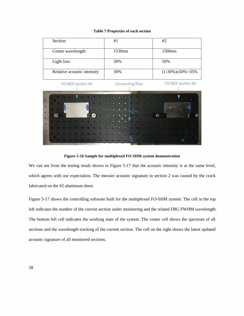
58
Table 7 Properties of each section
Section #1 #2
Center wavelength 1530nm 1560nm
Light loss 30% 50%
Relative acoustic intensity 30% (1-30%)x50%=35%
Figure 5-16 Sample for multiplexed FO-SHM system demonstration
We can see from the testing result shown in Figure 5-17 that the acoustic intensity is at the same level,
which agrees with our expectation. The messier acoustic signature in section 2 was caused by the crack
fabricated on the #2 aluminum sheet.
Figure 5-17 shows the controlling software built for the multiplexed FO-SHM system. The cell in the top
left indicates the number of the current section under monitoring and the related FBG FWHM wavelength.
The bottom left cell indicates the working state of the system. The center cell shows the spectrum of all
sections and the wavelength tracking of the current section. The cell on the right shows the latest updated
acoustic signature of all monitored sections.

59
Figure 5-17 LabVIEW controlling software for the multiplexed FO-SHM system
Conclusion
A multiplexable all-fiber-optics structure health monitoring system was presented in this phase. In the
demonstration of this system, the temperature, strain, thickness changes of an aluminum sample were
quantitatively associated with the FBG spectrum shift and the peak shifts in its acoustic signature. The
occurrence of an artificial crack was related to the appearance of new peaks in the acoustic signature. The
multiplexing capability was also preliminarily demonstrated by the acquisition of spectrum information
and acoustic signatures from an FO-SHM network containing two cascaded nodes. Despite that the
concept of FO-SHM has been brought up for several years, to our best knowledge, this is the first
experimental realization and demonstration of such a system.
The demonstrated temperature range is from 24oC to 60oC, which is the allowed working temperature of
the epoxy used in the FO-SHM node. By changing the epoxy to a high temperature adhesive such as a
ceramic adhesive, this system is expected to be able to reach much higher temperatures.

60
6 High temperature FO-SHM element surface attachment design,
simulation, and test
The work presented in this section serve as preparations for the final demonstration in a harsh
environment. The preliminary high temperature tests and simulation were focused on the final
demonstration material – P91 pipes. Several different surface attachment methods and adhesives were
tested and analyzed towards improving the high temperature survivability. Type-II FBG was also
fabricated and tested in this phase.
Identifying the structure health monitoring target material
P91 is the standard name for pipes made from T91 grade steel and it is widely used in the power industry.
We believe this is also the reason that DOE requested the final demonstration of this project be performed
on this material. According to our market search, the sizes of these pipes used in the power industry are
diverse in terms of diameter but the wall thickness is usually around or less than an inch. Because it is
difficult to conduct experiment on pipes with very large diameter in our lab, we decided to use small
diameter pipes for our experiment and demonstration. To be able to generate more versatile results, pipes
with different wall thickness were purchased for their potential usage in this project. The pipes we
acquired and stored in our lab is shown in Figure 6-1. The wall thickness range is from 1/4 inch to 1/2
inch.
These pipes were used throughout the research process and in the final demonstration to test and
demonstrate the capability of the developed FO-SHM system. However, the usage of the FO-SHM
system developed in this project is not necessarily limited to these pipes. It can be directly used on other
shapes/materials, or be deployed with modifications if needed.
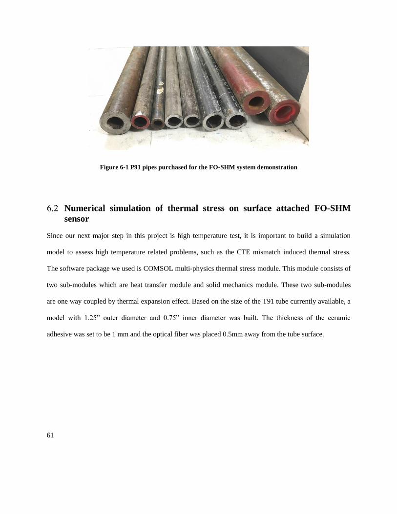
61
Figure 6-1 P91 pipes purchased for the FO-SHM system demonstration
Numerical simulation of thermal stress on surface attached FO-SHM
sensor
Since our next major step in this project is high temperature test, it is important to build a simulation
model to assess high temperature related problems, such as the CTE mismatch induced thermal stress.
The software package we used is COMSOL multi-physics thermal stress module. This module consists of
two sub-modules which are heat transfer module and solid mechanics module. These two sub-modules
are one way coupled by thermal expansion effect. Based on the size of the T91 tube currently available, a
model with 1.25” outer diameter and 0.75” inner diameter was built. The thickness of the ceramic
adhesive was set to be 1 mm and the optical fiber was placed 0.5mm away from the tube surface.

62
Figure 6-2. Simulation model.
Due to the size difference between the tube, adhesive, and silica fiber, each section was meshed
differently to ensure accurate result while saving calculation time. As shown in Figure 6-3, the tube has
the roughest mesh size. The mesh on the adhesive is finer, which gives it 5 layers of mesh. The silica fiber
has the finest mesh which is 4 mesh per cross section.

63
Figure 6-3. Mesh for FEM analysis.
The material properties used during the simulation are listed in Table 8. The values for silica and steel
come from the COMSOL material library and the values for ceramic adhesive come from the adhesive
manufacture.
Table 8 Material properties for thermal stress simulation
The T91 pipe is able to work continuously up to about 650 oC, and this is set as the working temperature
in the simulation. Figure 6-4 shows the simulation result in the form of Von-Mises stress. Von-Mises
stress is widely used as a criterion to decide whether or not a material will fail. If the maximum value of
Von-Mises stress on a piece of material is smaller than the yield strength of this material, it will not
deform, or vice versa. As shown in Figure 6-4, most of the stress is concentrated around the adhesive. The
majority part of the tube body has zero stress because its thermal expansion is not constrained in the
model.

64
Figure 6-4. Von-Mises stress of the whole model.
The stress and strain distributions in different sections are shown in Figure 6-5. Figure 6-5 (a) shows that
the highest stress is located around the corner, suggesting that sharp corners and edges should be avoided
in the sample fabrication. And the highest Von-Mises stress (1720 MPa) is higher than the yield strength
of T91 (415 MPa). Figure 6-5 (b) shows the strain along the fiber axis instead of stress, with the highest
value of 6.55 m at the center of the fiber. It is known that standard silica fiber has a yield strain about 1%
[35], so the fiber breakage may not be our main concern. Figure 6-5 (c,d) shows that the highest Von-
Mises stress is located around the corner at the value of 4050 MPa, which is much higher than its yield
strength (20 MPa). This also suggests that sharp corners should be avoided in real sample preparation.
Based on these values, in a high temperature environment, the most vulnerable part of this surface
attached sensor will be the ceramic adhesive due to its low yield strength. This suggests that other
alternative adhesive materials be searched for substitution.

65
Figure 6-5. (a) Von-Mises stress on the tube; (b) Strain along the fiber axis; (c) Top view of
Von-Mises stress distribution on the adhesive; (d) Bottom view of Von-Mises stress
distribution on the adhesive.
High temperature test of surface attached FO-SHM elements (ceramic
adhesive)
6.3.1 The first surface attachment method
In this section, we prepared a P-91 sample with an FO-SHM element attached on the surface by a high
temperature ceramic adhesive. We are familiar with this adhesive and know that it can reach a
temperature over 1000oC so it became the first candidate we tested for high temperature FO-SHM
element attachment.

66
The FO-SHM element was surfaced attached to a T91 tube with the high temperature ceramic adhesive
purchased from COTRONICS CORP. The surface was polished with 400 grit sandpaper prior to applying
the adhesive for stronger bonding. The width of the applied adhesive was around 1.5mm and the length
was about 5mm. The adhesive was firstly at the room temperature for 4 hours before the final curing at
65o C. Before heated up to high temperature, the lead-in/out fiber was secured by blue tapes on the surface.
The FBG used in this FO-SHM element is a -3dB type-I grating, due to the lack of type-II FBG
fabrication capability at that time.
Figure 6-6. FO-SHM element surface attached to a P91 pipe by high temperature ceramic
adhesive.
In this test, the P-91 sample was heated inside a high temperature furnace. The first procedure was to fully
cure the adhesive, which is to maintain the furnace temperature at 65oC for two hours. After this
procedure, the furnace was stabled at 100oC, 200oC and 300oC each for 2 hours. This ensured that the
sample temperature is consistent with the furnace temperature setting. The FO-SHM signal was recorded
at these four temperature points by the LabVIEW controlling software. At 300oC, we noticed that the
FBG spectrum was distorted, so we stopped this high temperature test to inspect potential fiber breakage.
The FO-SHM element looked intact by visual observation after cooled to room temperature as can be
seen from Figure 6-7. The adhesive bonding was relatively strong, but the FBG adhesive section could be
intentionally pulled off from the pipe. The adhesive was then carefully observed under the microscope

67
and several cracks were found as shown in Figure 6-8. As the crack may induce irregular strain
distribution around the FBG section, this can be one of the causes for the FBG spectrum distortion.
Figure 6-7 Surface attached FO-SHM element after the high temperature test
Figure 6-8 Ceramic adhesive after heating up to 300o C
As shown in Figure 6-9, the AE changes at different temperature points, which should be caused by the
temperature dependence of the elastic wave speed. Besides that, the signal strength is not stable when the
temperature changes. This unexpected phenomenon is related to the irregular shape change of the FBG
spectrum, which was observed during the heating up procedure.

68
Figure 6-9 Signal of the surface attached FO-SHM element at different temperature points
To further study the causes of the FBG distortion in a high temperature environment, a second test was
performed on the same P91 pipe, but with only the FBG section attached. The test followed a similar
procedure as the first test, with the temperature range extending to 650o C.

69
Figure 6-10 FBG spectrum during the second high temperature test
As we can see in Figure 6-10, the FBG spectrum experienced an irregular distortion/broadening at a
temperature lower than 350o C and returned to normal shape after the temperature passing 400o C. Besides
that, the reflection peak intensity dropped as the temperature steadily increased. The second phenomenon
was a known effect when a type-I FBG is used at high temperature. This issue is mainly due to dopant
diffusion and strain relaxation, and should be avoided in our final demonstration by replacing the type-I
FBG with type-II FBG. As for the irregular FBG spectrum distortion, possible cracks as shown in Figure
6-8 can be one cause. Another major cause should be the non-uniform strain distribution induced by
thermal stress, this will be illustrated by the following simulation results.

70
Figure 6-11 (a) Simulation model with surface attached FBG heated to 600o C; (b,c) Non-
uniform strain distribution along the silica fiber; (d) Simulation result of FBG spectrum
with non-uniform strain.
The same COMSOL simulation model shown in the previous section was used, however, the focus was
put on the strain distribution on the fiber instead of the highest von Mises stress. As shown in Figure 6-11
(b, c), after heated to high temperature, the strain on the fiber shows a non-uniform distribution. This non-
uniform distribution is caused by the edge of the adhesive, which should transform to a flatter distribution
if the adhesive is much longer than the FBG inside it. FBG with these strain distributions at different
temperature points were then simulated with transfer matrix method to give the predicted spectrums as
shown in Figure 6-11 (d). Comparing the experimental results in Figure 6-10 and simulation results in

71
Figure 6-11 (d), it can be seen that the first several spectrums in the experiment agree with the simulation
results pretty well in terms of shape broadening/distortion. However, the experimental spectrum
recovered its normal shape after 400o C. This may be caused by the release of the holding force between
the ceramic adhesive and the silica fiber. Because the thermal expansion coefficient of the ceramic
adhesive (8.1e-6/K) is larger than the CTE of silica (0.55e-6/K), the thermal mismatch may cause the
bonding to be loose at a higher temperature, thus weakening the non-uniformity of the strain distribution
on the silica fiber.
Based on these experimental findings and simulation predictions, we proposed and tested a surface
embedment design, intended to solve the cracking issues and achieve a more stable FBG spectrum during
high temperature environment.
6.3.2 The second surface attachment method
In this design, the whole optical fiber was buried into a pre-cut slot on the pipe by the same ceramic
adhesive used in the previous section. Based on the simulation results from the previous section, the high
temperature thermal strain should be uniform along the FBG because the adhesive length is much longer
than the FBG length. In addition, we hope this can also avoid crack formation in the adhesive.
As shown in Figure 6-12, a thin slot with about 1mm radius will be cut on the surface of the workpiece.
The optical fiber holding the FO-SHM element will be placed in the slot and sealed with ceramic
adhesive. To eliminate shape edges and irregular thermal stress distribution, overfilled adhesive will be
scraped off and the finished surface of the adhesive will be flat and smooth.

72
Figure 6-12 New schematic of FO-SHM element embedment
The simulation results acquired with COMSOL are shown in Figure 6-13. As our intuition predicts, the
strain distribution on the center part of the fiber (where the FBG is at) is basically flat, which means that
the FBG spectrum distortion/ broadening will be minimized as the temperature rise.
Figure 6-13 COMSOL simulation result of thermal strain distribution at 200o C

73
Figure 6-14 Full embedment sample preparation and new large volume tube furnace used in
the test
Figure 6-14 shows the fabrication process of a P91 testing sample containing a full embedded FBG fiber
link. A shallow 90 degree V groove was cutting on the P91 pipe with a square end mill as shown in
Figure 6-14 (A). The depth of the V-groove was about 0.5mm. Then the optical fiber containing the FBG
section was placed inside the V-groove and sealed by ceramic adhesive as shown in Figure 6-14 (B). The
adhesive was then cured at room temperature for 4 hours following the instruction of the adhesive
manufacturer. After this step, the adhesive became solid and the excessive amount of adhesive which
stuck out of the V-groove was polished off by sand paper. Figure 6-14 (C) shows the sample after
polishing. This testing sample was then placed inside a new large volume tube furnace as shown in Figure
6-14 (D). The heating procedure started with 2 hours at 150 oC which served as the final curing process
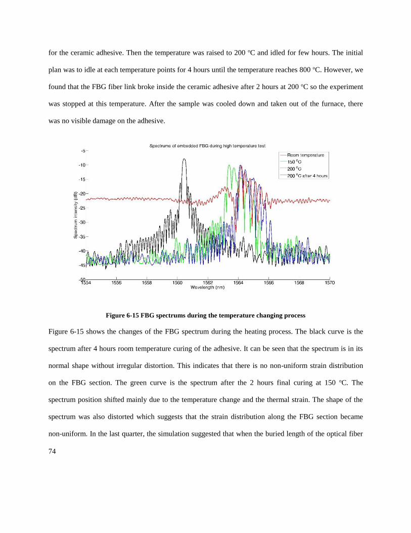
74
for the ceramic adhesive. Then the temperature was raised to 200 oC and idled for few hours. The initial
plan was to idle at each temperature points for 4 hours until the temperature reaches 800 oC. However, we
found that the FBG fiber link broke inside the ceramic adhesive after 2 hours at 200 oC so the experiment
was stopped at this temperature. After the sample was cooled down and taken out of the furnace, there
was no visible damage on the adhesive.
Figure 6-15 FBG spectrums during the temperature changing process
Figure 6-15 shows the changes of the FBG spectrum during the heating process. The black curve is the
spectrum after 4 hours room temperature curing of the adhesive. It can be seen that the spectrum is in its
normal shape without irregular distortion. This indicates that there is no non-uniform strain distribution
on the FBG section. The green curve is the spectrum after the 2 hours final curing at 150 oC. The
spectrum position shifted mainly due to the temperature change and the thermal strain. The shape of the
spectrum was also distorted which suggests that the strain distribution along the FBG section became
non-uniform. In the last quarter, the simulation suggested that when the buried length of the optical fiber

75
is much longer than the length of the FBG, the thermal strain should be evenly distributed through the
FBG section. The disagreement between the simulation result and this experiment result can be caused by
two reasons. Firstly, the cured ceramic adhesive was not perfectly isotropic. Secondly, a not perfectly
controlled polishing process generated a non-uniform cross section shape of the adhesive around the FBG
section. At the time that the temperature just reached 200 oC, the FBG spectrum (blue curve) shifted but
remained similar shape to the spectrum at 150 oC. However, after about 2 hours at this temperature, the
lower boundary of the spectrum (red curve) suddenly jumped up from -45 dB to -22 dB which indicates a
breakage in the fiber link.
Low CTE metallic adhesive based FO-SHM sample high temperature test
Based on the results acquired from the previous section, we did more market search and found one high
temperature metallic adhesive with lower CTE compared to what we previously used. During our tests,
we found this adhesive providing stronger bound to both the P91 pipe and the silica fiber. In this section,
we present the AE analysis with FO-SHM element attached on a P91 pipe by this new adhesive and its
high temperature test results. Relatively short length of adhesive was used for the surface attachment of
the FO-SHM element.
Based on the previous two sets of experiment, we proposed a new embedment plan featuring short section
attachment, stainless tube protection and low CTE metallic adhesive. Firstly, two pieces of small diameter
stainless tube are surface attached to a P91 pipe by high temperature adhesive. These two tubes are placed
in-line with each other and separated by a distance slightly larger than the length of the FBG section. The
two optical fibers containing the FBG and the acoustic generation structure will be placed inside the
stainless protection tubes. The FBG section will be aligned in the gap between the two tubes and the
acoustic generation unit will be certain distance from the FBG (hidden in one of the tubes). Finally, a low

76
CTE metallic adhesive (CTE=4e-6 /K) will be applied to both the FBG section and the surface area of the
tube section covering the acoustic generation unit. The structure is illustrated in Figure 6-16.
Figure 6-16 New FO-SHM embedment plan
A P91 pipe with 28.8mm OD and 5mm wall thickness was used in the following test sets. Firstly the AE
signature was obtained using the EFPI sensor and laser direct illumination method. Figure 6-17 shows
two different test conditions. In the first case, the EFPI fiber and the acoustic excitation fiber were placed
at the same angle on the pipe, i.e., a line connecting these two points will be parallel to the axis of the pipe.
In the second case, the acoustic excitation fiber was placed to a different angle as the EFPI fiber remained
in the same location.

77
Figure 6-17 Experiment setup for AE signature acquisition on a P91 pipe with EFPI sensor
and direct laser illumination acoustic generation
From Figure 6-18, we can see that the direct surface waves contribute to the most obvious peaks in the
AE signatures. This agrees with the experimental results discussed in the previous section. The 1st order
direct surface wave travels directly from the excitation point to the detection. The 2nd order direct surface
waves travel an additional round on the pipes from two directions. In case (a), the additional paths for the
two directions were the same so the two 2nd order waves combined into a larger peak. In case (2), since
the excitation point was placed at a different angle compared to the detection point, the symmetry was
broken and the additional paths for the two directions differed. As a result, two individual peaks can be
observed in the AE signature.

78
Figure 6-18 AE signatures acquired in the first test set
The second test set was done by attaching an FBG on the P91 pipe with a low CTE high temperature
metallic adhesive. A stainless tube was also used for fiber protection as designed in the last quarter.
Figure 6-19 (a) shows the materials and equipment for making such adhesive. Figure 6-19 (b) shows the
experiment setup for acquiring AE signature on the P91 pipe with surface attached FBG and direct laser
illumination acoustic generation. In this test set, the laser illumination point was placed at the same angle
as the FBG on the P91 pipe, and the distance between these two points was adjusted.
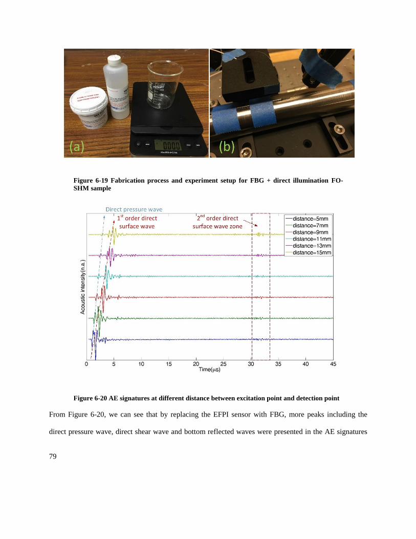
79
Figure 6-19 Fabrication process and experiment setup for FBG + direct illumination FO-
SHM sample
Figure 6-20 AE signatures at different distance between excitation point and detection point
From Figure 6-20, we can see that by replacing the EFPI sensor with FBG, more peaks including the
direct pressure wave, direct shear wave and bottom reflected waves were presented in the AE signatures

80
(direct shear wave and bottom reflection not marked). Also, since the acoustic excitation point and the
acoustic detection point were at the same angle on the pipe, the 2nd order direct surface waves were
combined. To get cleaner 2nd order surface wave peaks, the angle for the acoustic generation and
detection point were slightly separated in the final test set.
In the final test set, the distance between the excitation point and the detection was set to 10 mm. Also the
direct illumination acoustic excitation point was moved to a slightly different angle on the pipe. In Figure
6-22 (a) we can see that this generated two cleaner 2nd order direct surface wave peaks as we expected.
Then the end of the direct illumination fiber was attached to the surface of the P91 pipe and surrounded
by the low CTE adhesive. Another protection tube was used to secure both optical fibers on the pipe. This
step completed the final state of a single FO-SHM sensing node on a P91 pipe.
Figure 6-21 Completed state of the FO-SHM node on a P91 pipe
The AE signature for the completed FO-SHM sensing node on a P91 pipe is shown in Figure 6-22 (b). As
compared to Figure 6-22 (a), more bottom reflection peaks can be observed. This is possibly due to the
difference in acoustic generation. It appears that confining the laser energy inside its metallic surrounding
generates stronger body wave as compared to the surface illumination acoustic generation method. In the
final demonstration, the direct surface waves will be used for temperature calibration and the bottom
reflected waves will be used for corrosion-induced thickness change measurement.
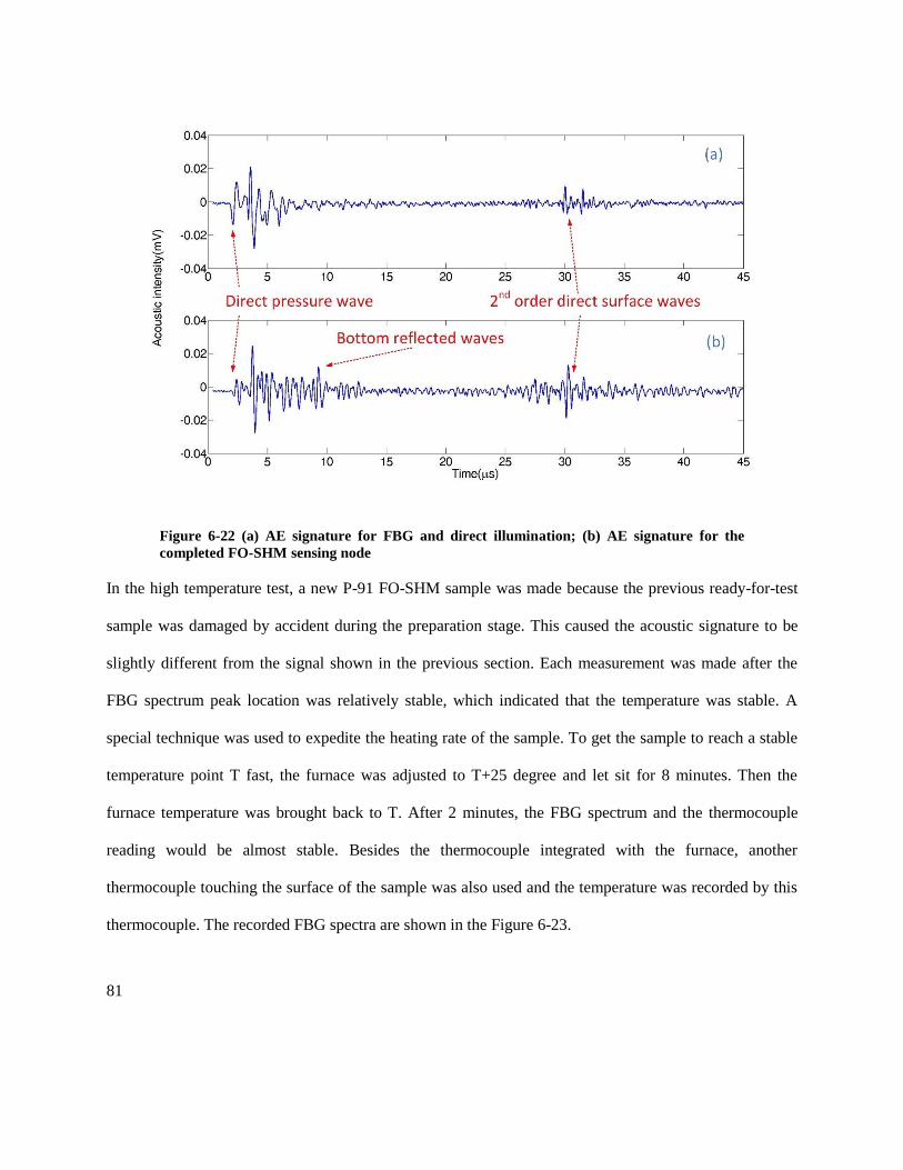
81
Figure 6-22 (a) AE signature for FBG and direct illumination; (b) AE signature for the
completed FO-SHM sensing node
In the high temperature test, a new P-91 FO-SHM sample was made because the previous ready-for-test
sample was damaged by accident during the preparation stage. This caused the acoustic signature to be
slightly different from the signal shown in the previous section. Each measurement was made after the
FBG spectrum peak location was relatively stable, which indicated that the temperature was stable. A
special technique was used to expedite the heating rate of the sample. To get the sample to reach a stable
temperature point T fast, the furnace was adjusted to T+25 degree and let sit for 8 minutes. Then the
furnace temperature was brought back to T. After 2 minutes, the FBG spectrum and the thermocouple
reading would be almost stable. Besides the thermocouple integrated with the furnace, another
thermocouple touching the surface of the sample was also used and the temperature was recorded by this
thermocouple. The recorded FBG spectra are shown in the Figure 6-23.

82
Figure 6-23 FBG spectrum during high temperature test
It can be seen that the FBG spectrum shifts to the right as the temperature rises and the peak intensity
slowly drops. The drop in peak intensity is due to the usage of a type-I FBG. We can see that up to 500oC
the FBG has retained its shape very well and is starting to change shape when reaching 550 oC. This is a
significant improvement compared to the previous sample under high temperature test and has confirmed
our prediction that a low CTE adhesive will help prevent inadvertent alteration to the shape of the FBG
spectrum. In the final demonstration, we will improve the shape uniformity of the adhesive applied and
hopefully increase the temperature threshold where the FBG spectrum turns irregular.
The acoustic signatures generated during the test are shown in the Figure 6-24, and their intensities are
adjusted according to the FBG intensity. It can be seen that the direct pressure wave maintains its shape
and intensity very well and can be used for temperature detection. An increase in the low-frequency

83
vibration of the acoustic signature was unexpected. This can be viewed in Figure 6-25 where the FFT
information of the acoustic signature is shown.
Figure 6-24 Acoustic signatures during the high temperature test, intensities calibrated by
their relating FBG intensities
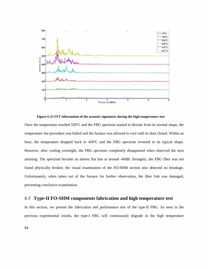
84
Figure 6-25 FFT information of the acoustic signatures during the high temperature test
Once the temperature reached 550oC and the FBG spectrum started to deviate from its normal shape, the
temperature rise procedure was halted and the furnace was allowed to cool with its door closed. Within an
hour, the temperature dropped back to 450oC and the FBG spectrum reverted to its typical shape.
However, after cooling overnight, the FBG spectrum completely disappeared when observed the next
morning. The spectrum became an almost flat line at around -40dB. Strangely, the FBG fiber was not
found physically broken; the visual examination of the FO-SHM section also detected no breakage.
Unfortunately, when taken out of the furnace for further observation, the fiber link was damaged,
preventing conclusive examination.
Type-II FO-SHM components fabrication and high temperature test
In this section, we present the fabrication and performance test of the type-II FBG. As seen in the
previous experimental results, the type-I FBG will continuously degrade in the high temperature

85
environment, thus is not suitable for our high temperature application. To solve this problem, type-II FBG
was proposed to be used as the acoustic detection unit, which was reported to work stably at 1000oC [22].
While the type-I FBG is formed by refractive index change induced by the photo-sensitive process in the
germanium doped core, the type-II grating is formed by inscribing micro voids inside the fiber core with
very high intensity laser. A femtosecond laser point by point FBG inscription setup was built in our lab to
write this type of grating. In this system, the fs laser pulse is focused by a 100X objective lens to inscribe
voids with less than 1 um diameter inside the fiber core. A high precision air bearing stage holding the
optical fiber is moving with a stable speed during the inscription process. The periodical accuracy is
ensured by the accuracy of the repeat rate of the femtosecond laser and the stable moving speed of the air-
bearing stage. The typical parameters we used for FBG inscription are shown in Table 9. The setup is
shown in Figure 6-26 and the result of typical grating inscribed by this system is shown in Figure 6-27.
Table 9 Typical type-II FBG inscription parameters
Femtosecond repeat
rate 1 kHz FBG period 1.07 um
Pulse energy 0.4 uJ Fiber moving speed 1.07 mm/s
Pulse width 125 fs FBG length 2 mm

86
Figure 6-26 (a) The Libra femtosecond laser; (b) The point-by-point type-II FBG inscription
system.
Figure 6-27 (a) Type-II FBG spectrum; (b) The periodical structure of the type-II FBG
under 100X microscope.
A P-91 sample with surface attached type-II grating was then fabricated with the metallic adhesive. This
sample was tested from 25oC to 700 oC. The FBG spectrum distortion started to show at 600 oC and the
FBG broke at 700 oC. From 25 oC to 500 oC, the FBG spectrum was stable in terms of the shape and peak
intensity. This result is shown in Figure 6-28.

87
Figure 6-28 Surface attached type-II FBG high temperature test result
A similar setup with 20X objective lens was built to fabricate the acoustic excitation unit used in the FO-
NDE element. This lower magnification lens was used to generate larger size voids for the higher light
scattering ratio. When using the parameters shown below, the size of the voids is about 10 um.
Table 10 Parameters used for the inscription of the acoustic generation type-II voids
Distance between
voids
40 um Laser pulse energy 8 uJ
Position of voids Center of the
core
Pulses for each
voids
100
Total length 1mm Total loss 10%
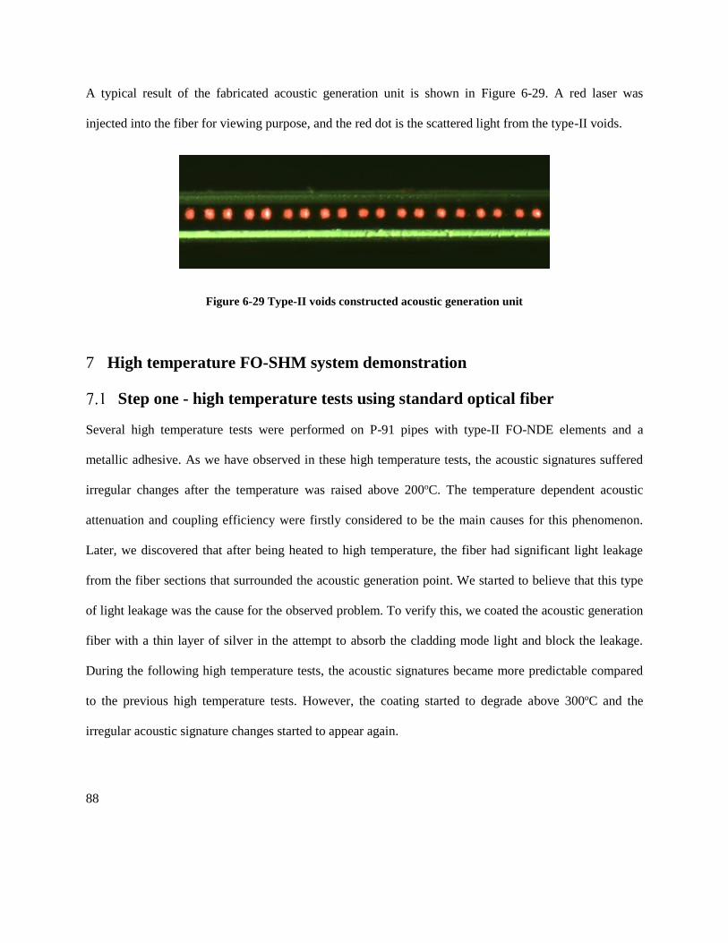
88
A typical result of the fabricated acoustic generation unit is shown in Figure 6-29. A red laser was
injected into the fiber for viewing purpose, and the red dot is the scattered light from the type-II voids.
Figure 6-29 Type-II voids constructed acoustic generation unit
7 High temperature FO-SHM system demonstration
Step one - high temperature tests using standard optical fiber
Several high temperature tests were performed on P-91 pipes with type-II FO-NDE elements and a
metallic adhesive. As we have observed in these high temperature tests, the acoustic signatures suffered
irregular changes after the temperature was raised above 200oC. The temperature dependent acoustic
attenuation and coupling efficiency were firstly considered to be the main causes for this phenomenon.
Later, we discovered that after being heated to high temperature, the fiber had significant light leakage
from the fiber sections that surrounded the acoustic generation point. We started to believe that this type
of light leakage was the cause for the observed problem. To verify this, we coated the acoustic generation
fiber with a thin layer of silver in the attempt to absorb the cladding mode light and block the leakage.
During the following high temperature tests, the acoustic signatures became more predictable compared
to the previous high temperature tests. However, the coating started to degrade above 300oC and the
irregular acoustic signature changes started to appear again.

89
7.1.1 High temperature tests with standard 105/125m fiber
A typical sample is shown in Figure 7-1. During these tests, we found the acoustic signatures were not
consistent when heated above 200oC. In several cases, the position of the first pulse in the acoustic
signature moved forward in the time domain when temperature increased, which is against our prediction
because the speeds of elastic waves generally decrease when the temperature rises. A typical result of the
acoustic signature evolution is shown in Figure 7-2.
Figure 7-1 P-91 sample with type-II FO-NDE elements

90
Figure 7-2 Acoustic signature evolution in high temperature environment
By examining the samples after the high temperature tests, we discovered that the acoustic generation
fiber developed severe light leakage around the acoustic excitation point during the tests. This
phenomenon is shown in Figure 7-3. Due to these unwanted light leakage, the properties of the acoustic
source were significantly changed in high temperature environment, which rendered the acoustic
signature un-predictable.
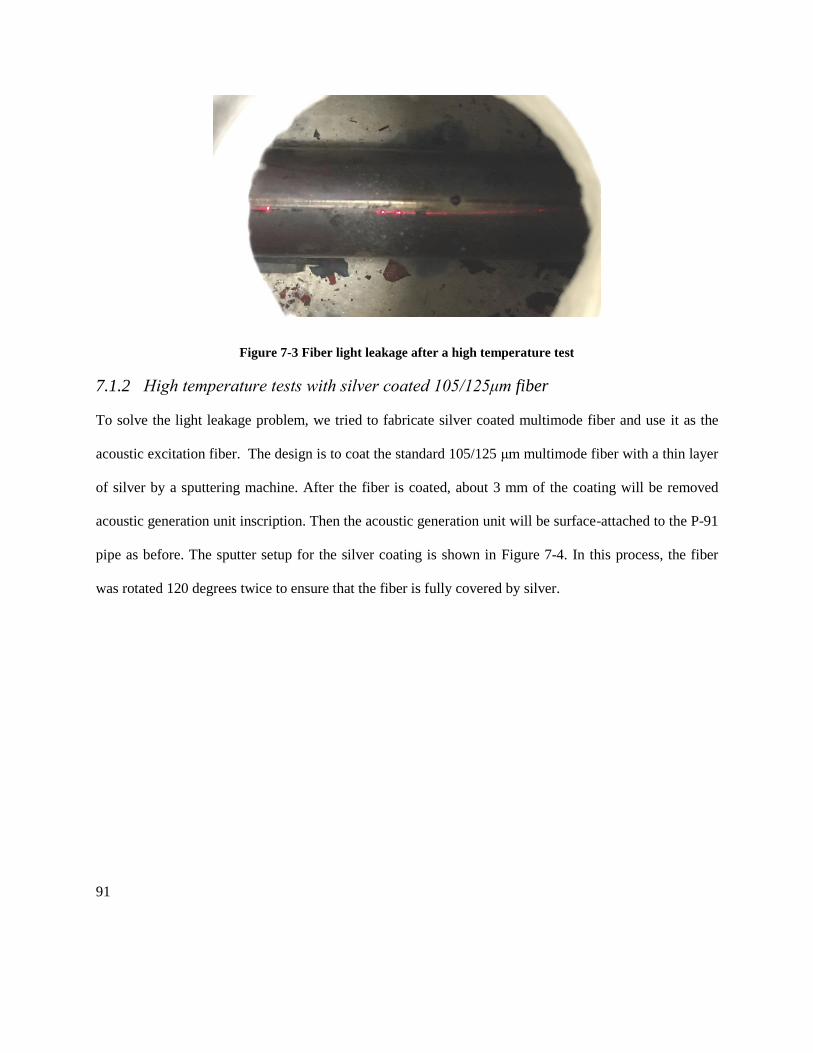
91
Figure 7-3 Fiber light leakage after a high temperature test
7.1.2 High temperature tests with silver coated 105/125μm fiber
To solve the light leakage problem, we tried to fabricate silver coated multimode fiber and use it as the
acoustic excitation fiber. The design is to coat the standard 105/125 μm multimode fiber with a thin layer
of silver by a sputtering machine. After the fiber is coated, about 3 mm of the coating will be removed
acoustic generation unit inscription. Then the acoustic generation unit will be surface-attached to the P-91
pipe as before. The sputter setup for the silver coating is shown in Figure 7-4. In this process, the fiber
was rotated 120 degrees twice to ensure that the fiber is fully covered by silver.

92
Figure 7-4 Silver coating fiber sputter setup
After the fiber was coated with the silver coating, a fiber section slightly longer than the type-II voids
section was de-coated, and this section was used for the acoustic generation unit inscription. The product
of this process is shown in Figure 7-5. The thickness of the silver coating is about 1 um and the length of
the type-II voids section is 2 mm.
Figure 7-5 Acoustic generation unit on silver coated fiber
With the silver coating fiber, several FO-NDE elements were fabricated and put through high temperature
tests. During these tests, it was found that the coating started to delaminate at around 300oC. As shown in
Figure 7-6, the scattering light started to appear at 300oC and became very strong at 600oC. The quality
and the thickness of the coating may be the cause for this phenomenon. However, we were still able to
confirm that the acoustic signature became more predictable below 400oC comparing to the experiment

93
results acquired with non-coating fiber. As shown in Figure 7-7, the acoustic signature maintains its own
shape well up to 300oC and shows some trailing pulses after the main envelope. A zoom-in view of the
main envelope as in Figure 7-8 shows that the first several pulses in the acoustic signature shifts
monotonically in the whole process, which should be caused by the temperature induced acoustic velocity
change.
Figure 7-6 (a) Light leakage at 300oC; (b) Light leakage at 600oC.

94
Figure 7-7 Overall view of the acoustic signature evolution with silver coated fiber

95
Figure 7-8 Zoom-in view of the front section of the acoustic signature evolution
Based on this result, we believe that solving the light leakage problem will bring significant improvement
to the readability of the acoustic signature in high temperature environment. And it is a necessary step to
achieve the goal of measuring environmental parameters for high temperature applications. To achieve
this, we acquired some commercial gold coated multimode fiber and fabricated the acoustic generation
unit on this fiber. Because the coating quality of the commercial gold coated fiber is higher and the fiber
is rated up to 700oC, the result was substantially improved as discussed in the next chapter.

96
Step two - high temperature tests using gold coated optical fiber
After confirming the importance of eliminating unwanted light leakage from the acoustic generation fiber,
we searched the market and purchased a gold coated 105/125 μm step index multimode fiber. The
thickness of the gold coating is 15 um, which makes the overall fiber diameter 155 um. This fiber is rated
up to 700oC which is sufficient for our application. Several tests were performed with this fiber replacing
the standard 105/125 μm fiber we used before. To fabricate the acoustic generation unit (AGU) on this
fiber, a portion of the fiber slightly longer than the AGU was de-coated. Figure 7-9(d) shows the AGU
after the type-II voids were inscribed. The AGU was then attached to a P-91 pipe with a metallic adhesive
as shown in Figure 7-9(e). To prevent unwanted light leakage, the metallic adhesive was slightly longer
than the de-coating area and contacted both ends of the gold coating. A completed P-91 sample is shown
in Figure 7-9(a). Four ceramic tubes were used to secure the fiber on the pipe, which allowed fiber sliding
and prevented fiber bending during the high temperature test. After heating to 600oC and cooling down to
room temperature, the FO-NDE element and the gold coating fibers were intact under visual observation
as shown in Figure 7-9(c).

97
Figure 7-9 (a) P-91 high temperature test sample with gold coated fiber FO-NDE element
attached; (b) Sample in the furnace; (c) FO-NDE element remains in good shape after
heating; (d) Acoustic generation unit on a gold coated fiber; (d) Acoustic generation unit
attachment on the P-91 pipe.
During the high temperature tests, we injected a red laser beam into the FO-NDE elements and observed
the sample from a hole on the top of the furnace. During several tests performed with the gold coated
fibers, no unwanted light leakage was observed. The acoustic signature evolution in one of these tests is
shown in Figure 7-10. The temperature induced peak shifts can be clearly observed on both the direct
surface Rayleigh waves and the surface waves that travel a full round on the pipe. The result also shows
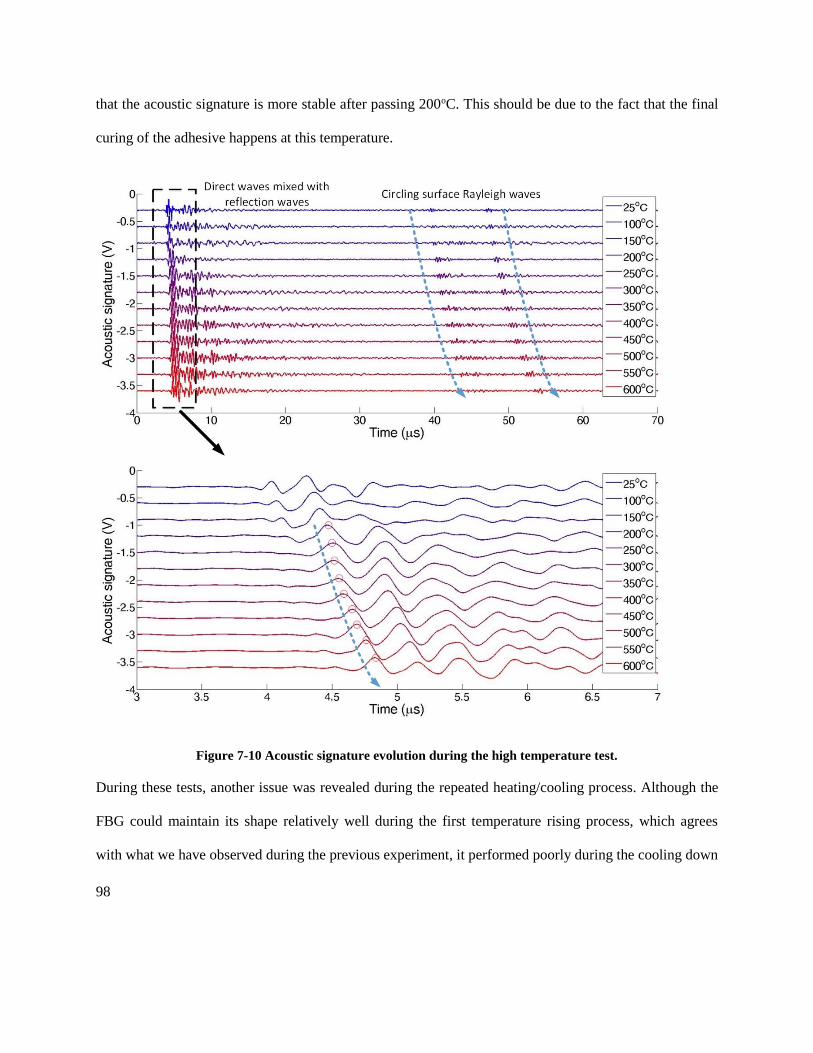
98
that the acoustic signature is more stable after passing 200oC. This should be due to the fact that the final
curing of the adhesive happens at this temperature.
Figure 7-10 Acoustic signature evolution during the high temperature test.
During these tests, another issue was revealed during the repeated heating/cooling process. Although the
FBG could maintain its shape relatively well during the first temperature rising process, which agrees
with what we have observed during the previous experiment, it performed poorly during the cooling down

99
process. One typical result is shown in Figure 7-11(a). During the cooling down process, the FBG
spectrum shows irregular changes and decrease in the peak reflectance. In addition, the FBG center
wavelength is not repeatable by comparison between the heating and the cooling processes. This can be
observed in Figure 7-11(b, c).
We suspect that the cause for this issue is the weak bonding between the metallic adhesive and the silica
fiber. During the heating up process, the fiber may slip inside the metallic adhesive due to the CTE
mismatch and the low bonding strength. In the cooling down process, the adhesive may shrink rapidly
and exert non-uniform stresses on the FBG and make the spectrum distorted. Although the occurrence of
this issue was somewhat random, we decided that this should be solved for the preparation of the long
term high temperature tests. In the next chapter, we will present an innovative upgrade to the current FBG
sensing structure which ensures long term stability and repeatability.

100
Figure 7-11 (a) FBG spectrums during a high temperature test; (b) FBG peak reflectance
evolution; (c) FBG peak wavelength evolution.
Step three - high temperature tests using FP-FBG sensing structure
7.3.1 Principle of FP-FBG

101
In this chapter, we replaced the type-II FBG with a type-II FP-FBG to eliminate the FBG spectrum
distortion experienced during the repeated temperature changing process. An FP-FBG is constructed with
two in-line FBGs separated by a certain gap distance, which determines the free spectral range (FSR) of
the FP cavity. Using a relatively large gap distance, such as 2 cm, an FSR around 50pm can be obtained,
which is much smaller than the FWHM of a traditional FBG. Because the FSR of an FP-FBG is smaller,
the acoustic detection sensitivity can be higher than an FBG. However, the most significant advantage of
using an FP-FBG for high temperature acoustic sensing is that the adhesive doesn’t need to be applied
directly onto the FBG. Instead, the adhesive can be applied anywhere between the two FBGs. This leaves
the FBGs free standing, which eliminates any possible thermal stress in the FBGs even at high
temperatures. A schematic of this design is shown in Figure 7-12 together with a simulated spectrum and
an actual spectrum acquired in the following experiments. Assuming the probe light enters the FP-FBG
from the left, the length of the FBG on the right is designed to be longer than the FBG on the left. This is
due to the consideration of type-II FBG transmission losses. If the lengths of the two FBGs are the same,
due to type-II FBG losses, the reflection from the right FBG will be significantly weaker than the left
FBG, which will result in a low FP fringe contrast. During the experiment, we did several tests and found
that a (0.5 mm FBG +2 cm gap +1.5mm FBG) type-II FP-FBG could give a good fringe contrast (> 50%).
The experimental result shown in Figure 7-12 actually has around 50% fringe contrast. The fringe
contrast seems lower than 50% only due to the limited CTS spectral resolution. Figure 7-13 shows a P-91
sample with the FP-FBG implemented for acoustic sensing. The adhesive between the FBGs is about
2mm long.
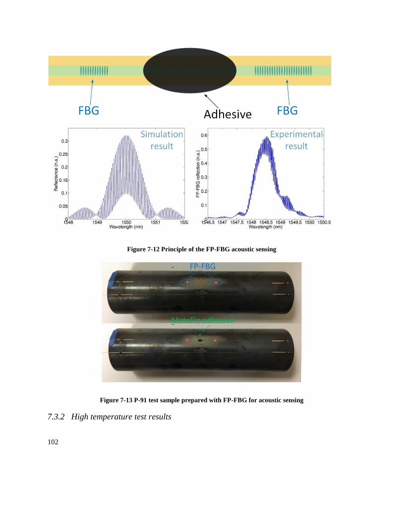
102
Figure 7-12 Principle of the FP-FBG acoustic sensing
Figure 7-13 P-91 test sample prepared with FP-FBG for acoustic sensing
7.3.2 High temperature test results

103
Figure 7-14 shows the spectrum evolution of the FP-FBG during one of the high temperature tests we
performed. It can be seen that the spectrum maintains its shape very well during the process and is highly
repeatable. The variance of the peak reflectance is less than 0.5 dB during the whole process. The peak
wavelength is recorded by filtering the spectrum and then using a centroid algorithm. The repeatability of
the peak wavelength is within 50 pm.
Figure 7-14 (a) FP-FBG spectrum evolution during a high temperature test; (b) Peak
reflectance evolution; (c) Peak wavelength evolution.
An acoustic signature evolution was also recorded and is shown in Figure 7-15. This result is similar to
what we have shown in the previous chapter. The surface waves traveling one round of the pipe show
good temperature dependent shifts in the time domain. The direct waves show good temperature
dependent shifts beyond 200oC.

104
Figure 7-15 Acoustic signature evolution during a high temperature test
We have demonstrated the operation of an innovative FO-NDE element at temperatures up to 600oC. The
spectrum is stable and repeatable which can be used to measure temperature. The acoustic signature is
stable in the high temperature environment, which also shows good and predictable temperature
dependent shifts in the time domain.

105
Corrosion, strain and crack tests
In this chapter, we will demonstrate the corrosion, strain and crack tests on a P-91 pipe in the room
temperature with the finalized FO-NDE structure described in the previous chapter.
7.4.1 Corrosion test
We used an electro-etching process to simulate the chemical corrosion that may happen inside a P-91 pipe
as shown in Figure 7-16(a). Before the process, the inside of the pipe was roughly polished to remove the
protection paint inside the pipe, which will prevent the corrosion from happening if not removed. After
the rough polishing, the inner surface was still very coarse and has many small dents on it. The chemical
used for the etching was a NaCl solution. The anode was connected to the pipe through a thin copper
sheet, and a metal rod was inserted into the pipe as the cathode. The current used for the etching was set
at 1.98 A. The solution was cycled after every few minutes to maintain the etching speed and remove the
debris. Due to the heat generated during the etching process, the acoustic signatures were each taken after
a long time cooling process. This brought the temperature of the sample back to the room temperature for
each acoustic signature measurement.
Figure 7-16 (a) Pipe inner surface electro-etching setup; (b) Acoustic signature evolution
during the corrosion process

106
The result is shown in Figure 7-16(b). Due to the roughness of the etched surface and the mixing of
bottom reflections and direct waves, the peak shifts in the “bottom reflection affected area” is irregular
and not monotonic. On the right of this area, where there should only be bottom reflections, a peak around
4.5 s is found to show monotonic shift to the left. The calculated wall thickness change is about 1.25%.
This test demonstrated that the occurrence and severity of corrosion can be indicated by the changes in
the acoustic signature. To achieve better result in the future, such as a major peak shifting monotonically
with corrosion thickness, longer acoustic pulse width may be used to reduce the negative effect of a poor
inner surface quality.

107
7.4.2 Strain test
In the strain test, we used a hydraulic pump jack to exert compressional force on the sample. The setup of
this test is shown in Figure 7-17. An OMEGA strain foil gauge was attached on the sample to provide a
strain reference in the axial direction.
Figure 7-17 Strain test setup
During this test, we measured the peak shift of a surface Rayleigh wave that travels two rounds on the
pipe. The location of this peak is around 83 s. As shown in Figure 7-18, this peak shifts monotonically
with the applied strain on the sample. The less-than-ideal linearity may be due to the fact that the strain
gauge is attached close to the end of the sample and the strain distribution near the end is non-uniform
and irregular.
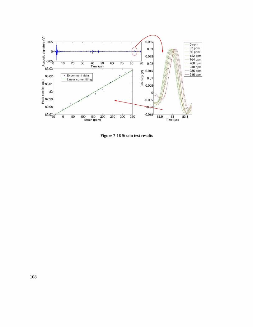
108
Figure 7-18 Strain test results

109
7.4.3 Crack test
In the crack test, we explored two methods. The first one is the industrial standard PLB test which only
used the AGU portion of the FO-NDE element. In this test, the acoustic detection was set to be triggered
by itself. A pencil lead was broken around 1 cm from the FO-NDE element and the recorded PLB signal
is shown in Figure 7-19.
Figure 7-19 PLB signal
The second test was the active crack detection which used the whole FO-NDE element. A dremel tool
with 0.5mm thickness was used to cut surface slits on the sample near the FO-NDE element. In this test,
two cracks were cut and they were located on the two different sides of the FO-NDE element. One of
them was parallel with the axial of the sample, the other one formed a 45 degree angle to the axial
direction.

110
Figure 7-20 Crack simulation setup and cut sample
The test result is shown in Figure 7-21. By calculating the difference between the acoustic signatures
before and after the slits cutting, we observed several new peaks. It should be noted that the peaks in the
shaded area are not generated by the cracks. Instead, they are due to a slight temperature difference
between these two sets of acoustic signatures.
Figure 7-21 Crack test results

111
Conclusions
In this project, we have proposed and demonstrated a surface attached active fiber optic sensing network
that can be used for structural health monitoring at high temperatures up to 600oC. Several optical fiber
based acoustic generation mechanisms were investigated and compared. The LIP based method has the
highest photo-acoustic conversion efficiency, but is mechanically weak when it is used in a fiber optics
structure and is not able to perform stably in a long term. The EDF based method is the most elegant
design which uses only one fiber, but has the lowest photo-acoustic conversion efficiency thus is not a
good choice for this project. The method we chose over the two is the scattering light based thermal
expansion method, which has both good photo-acoustic conversion efficiency and long term stability. A
complete bench-top sensing system based on this acoustic generation mechanism and the FBG acoustic
detection was designed, built and tested. Both quantitative multi-parameter monitoring and system
multiplexing were successfully demonstrated. Significant efforts were then devoted to applying this
system on a P-91 pipe placed in a high temperature environment. The challenges mainly arise from the
unwanted light leakage and the CTE mismatch between the fiber, the adhesive and the P-91 material. To
eliminate the unwanted light leakage from the acoustic generation fiber, which often made the acoustic
signature highly distorted, different types of metal coated fibers were tested. We finally chose the
commercial grade gold coated fiber because it offers stable operation even at high temperatures beyond
600oC. The CTE mismatch between the materials generated issues such as fiber breakage and FBG
spectrum irregular distortion during the repeated temperature changes. To solve these issues, different
types of high temperature adhesive were tested and we finally chose a Cotronics metallic based adhesive,
which has relatively low CTE and low Young’s modulus. In addition, we have changed the acoustic
sensing mechanism from the standard FBG acoustic sensing to an FP-FBG acoustic detection, which
avoids the physical contact between the FBGs and the adhesive. This provides a very stable and

112
repeatable high temperature sensing performance. Finally, the implemented fiber optic, sensor system
was demonstrated for the measurement of temperature, strain, cracks and corrosion. Based on our best
knowledge, this demonstrated method is the first technology of a kind that permits multi-parameter
measurement at temperatures up to 600 oC.

113
8 Guided elastic wave study for future research
Analytical model of guided elastic wave propagation
To prepare for the final demonstration which will be using ultrasonic structure health monitoring
technique on a P91 pipe, it is necessary to study the elastic wave generation and propagation on such a
structure. When the thickness of a pipe is much smaller than the acoustic wavelength and the tube
diameter, the elastic modes supported can be approximated by the modes supported by a thin plate [36],
which are SH modes and Lamb-type modes [23]. According to our online market search, most stocked
P91 pipes generally satisfy these conditions so we will use SH modes and Lamb modes to describe the
elastic wave propagation on thin-wall pipes in the future study.
The frequency equations for SH modes and Lamb waves can be deduced by the elastic motion equation
and stress-free boundary conditions. The results are[23]:
Here is the wave number, is the frequency, d is the thickness of the plate, SV is the shear wave
speed in this bulk material, LV is the shear wave speed in this bulk material, p and q are defined as
followed.
SH modes 2 2 2( ) ( ) , 0,1,2,3..........
S
nn
V d
(23)
Symmetric Lamb waves
2
2 2 2
tan( / 2) 40
tan( / 2) ( )
qd qp
pd q
(24)
Anti-symmetric Lamb waves
2 2 2
2
tan( / 2) ( )0
tan( / 2) 4
qd q
pd qp
(25)

114
Using MATLAB to solve these equations we acquired dispersion curves for these three modes, the results
are shown in Figure 8-1. The X axis of the dispersion curves is the product of the frequency and the
thickness of the tube, the Y axis is the phase velocity. It can be seen that when the thickness of the tube
changes, such as due to corrosion, these dispersion curves will shift and consequently change the acoustic
signature of a pipe. Therefore this provides a possible way to monitor the thickness of a thin-wall pipe.
Figure 8-1 Dispersion curves for symmetric Lamb waves (red curves), anti-symmetric Lamb
waves (blue curves) and SH waves (green curves)
FEM simulation of the guided elastic wave and experimental result
To study the elastic wave generated by laser heating, a simulation model was built with the COMSOL
thermal-elastic module. A thin-wall tube with 0.5” diameter and 0.5mm wall thickness was used as the
2 2 2 2 2 2( ) , ( )
L S
p qV V
(26)

115
testing workpiece. A 1 mm by 1 mm surface area was chosen as the heat source in-flow area, to represent
the laser heating area. The time profile of the in-flow heat was set to a Gaussian pulse with 50ns standard
deviation which agrees with the laser source we used in the experiment. Due to the fact that a P91
material can’t be found in COMSOL’s material library, the properties of standard steel AISI 4340 was
used in the simulation. As seen in Figure 8-2, the generated elastic waves propagate with circular wave
fronts.
Figure 8-2 COMSOL simulation result of elastic wave generation by laser heating
The propagation of the elastic waves was monitored in a surface point 1cm away from the source area.
The monitored value was the surface displacement in Y direction (normal to the surface). The result will
be shown together with an experimental verification result in the following section.
To verify the accuracy of the COMSOL simulation, a confirmatory experiment was conducted with direct
laser heating and EFPI sensing. A copper tube with very similar sizes to the simulation model was used in
the experiment. A multimode fiber which guided the high-intensity laser pulse pointed to the surface of
the tube with about 2mm distance from the surface, this generated a circular heating area with roughly 1
mm diameter. The polished end surface of a single-mode fiber was placed near the surface of the tube

116
(distance smaller than 1mm), served as the EFPI sensor that detects the surface displacement in the
normal direction. The laser used for acoustic generation is the 1064nm Nd:YAG laser with 50ns pulse
width and 0.3mJ pulse energy, the laser source used for EFPI is a tunable C-band laser.
Figure 8-3 Experiment setup for thin-wall tube elastic wave generation and detection
The normalized acoustic signatures from both the simulation result and the experimental result are plotted
in the upper graph in Figure 8-4. The features of these two plots are similar in terms of the transition from
several smooth vibrations to vibrations with higher frequency spikes. The lower graph in Figure 8-4
shows the Fourier transformations of these two acoustic signatures, and they are very similar. Although
these two acoustic signatures are similar, there is still a noticeable difference between them such as the
total time duration of the smooth vibration area. These differences should be caused by three reasons.
Firstly, the laser heating area in the simulation model is a rectangular area while in the experiment it is a
circular area. Secondly, the material used in the COMSOL model is stainless steel and the actual material
used is a certain type of copper. Finally, the mesh size in the simulation model may not be fine enough to
give a high accuracy prediction. The mesh used in the current simulation is in the fine grade and a single

117
run of the simulation takes about one day. In the next quarter, we will try higher mesh sizes and see if
they will produce more accurate results.
In all, we believe this model is good enough for preliminary experiment prediction, such as studying the
effect of changing tube thickness or cracks on the acoustic signature. This will save time for future
experiment and help prepare the final demonstration.
Figure 8-4 Results comparison between the COMSOL simulation result and the
experimental result

118
9 Introduction to fiber optic guided laser micromachining (GLMM)
In recent years, there has been an increasing need for high aspect ratio micro hole drilling in numerous
applications such as aviation, aerospace, automobile, electronics, medical devices and MEMS [37-39].
For example, deep micro holes are used as turbine blade cooling channels and diesel fuel injection
nozzles to improve engine energy efficiency. In medical applications, high aspect ratio micro holes are
highly desirable for drug delivery, medical implants and bone surgeries. Typical requirements of these
drilling applications include micron scale hole diameters, high aspect ratios and drilling versatility.
Currently, laser beam micromachining (LBMM) is being used for micro hole drilling both in academic
area and commercially. With sufficiently high laser power, LBM practically works on all kinds of
material due to the nature of the laser ablation process. For micro hole drilling, the Rayleigh range of the
laser beam, where the beam spatial profile is considered collimated and non-tapered, is generally used.
However, the maximum aspect ratio of the machined micro holes is limited to be less than several tens
[40-43] due to the short Rayleigh range in a tightly focused laser beam and the accumulation of debris.
In this work, we present an innovative laser micromachining method which uses optical fiber guided laser
beam instead of the free space laser beam to break the aspect ratio barrier rooted in the traditional LBMM
method. The key concepts of this optical fiber guided laser micromachining (GLMM) technology include
two aspects: 1) An optical fiber guides high-intensity laser pulses to the drilling front, where the solid
state material is transformed into nanometer particle debris by laser ablation. 2) Fiber holes are utilized to
continuously flush off debris and the heat-generated gaseous bubbles, maintaining a liquid-filled drilling
front condition.

119
Figure 9-1 Key principle of optical fiber guided micro drilling and side hole debris flushing
A cross-sectional views of such a GLMM process is shown in Figure 9-1. The process starts with
coupling a high intensity pulsed laser beam into the center core of a multimode fiber with micro holes on
it, here a side-hole fiber is used as an example. After transmission inside the fiber core, the laser beam
exits from the fiber end and expands to form a “drilling tip” to remove unwanted material from the
workpiece through laser ablation. The typical laser damage threshold (LDT) of a step-index silica fiber is
around 1-3 GW/cm2 [44] for 1064nm laser pulse with nanosecond duration, which is higher than the

120
plasma thresholds of most materials. For example, the plasma threshold for metals are general in the
range of 0.2-0.5 GW/cm2 [45], polymers are general in the range of 0.001-0.009 GW/cm2 [46]. Because
of this, GLMM is expected to be applicable to all metallic materials and most non-metallic materials.
During the laser ablation process, the material in the plasma state radiates atomic and ionic emission [47-
49], known as plasma emission. This plasma emission can be collected by the fiber core and sent back for
analysis, which provides information about the material and the drilling condition. As the drilling front is
filled with liquid, the plasma plume cools down to form nanoscale particle debris which suspends in the
surrounding liquid [50, 51]. In general, these debris particles have a diameter smaller than 1 μm [51, 52]
when a nanosecond laser pulse is used. By designing the side gap to be larger than 1 μm, the debris can be
easily flushed out.
10 Simulations of the GLMM process
Modelling the shape of a static “drilling tip”
To show that it is possible to design such a fiber structure for material removing and debris flushing, a
simulation was conducted to study the relationship between the relative in-fiber laser intensity, core NA,
the shape of the “drilling tip” and drilling ratio. Relative laser intensity is the normalized intensity over
the laser ablation threshold intensity of the target material. The shape of the “drilling tip” is defined by the
boundaries where the relative laser intensity equals a certain value, the outermost boundary is where the
relative laser intensity equals one. The drilling ratio is defined as the ratio of the diameter of the “drilling
tip” over the diameter of the fiber core. We use ray optics to analyze the output laser intensity profile
from a multimode fiber core, which represents the “drilling tip”. The laser reflection from the hole
boundary is ignored in the current model. A “drilling tip” shape obtained with 0.22 core NA and water
surrounding is shown in Figure 10-1. The result shown in Figure 10-1(b) is obtained with the relative in-
fiber laser intensity set to 7, which is a reasonable number for metallic materials. It is shown that the NA

121
of the fiber core doesn’t affect the drilling ratio much within the typical range for pure silica core, which
is from 0.2 to 0.4. And the drilling ratio (about 1.75) allows a flexible design of the fiber side hole pattern.
The results in Figure 10-1(c) is acquired with variable relative in-fiber laser intensity and 0.22 NA, which
shows that higher in-fiber laser intensity results in higher drilling ratio and larger bottom clearance.
Figure 10-1 Simulation result of the cross-section shape of a "drilling tip" with different
boundaries; the value on each boundary represents the normalized laser intensity on that
boundary relative to the laser intensity in the fiber core; surrounding medium is water with
refractive index. (a) Simulation result of the dependent relationships of drilling ratio and
bottom clearance on fiber NA (b) Simulation result of the dependent relationships of drilling
ratio and bottom clearance on the relative in-fiber laser intensity
Dynamic simulation of the GLMM drilling process
To build a dynamic model which simulates the drilling process, we investigated how the laser pulse
properties affect the laser ablation depth, i.e., the thickness of the material removed by a single laser pulse.
Laser ablation is a complex process and the key concepts include laser absorption, heat transfer, material
melting, material evaporation, phase explosion, laser intensity attenuation through plasma [53-62], and
the interaction between the plasma plume and surrounding liquid [50-52]. In this study, we combined the
experimental ablation depth result from another work [58] with our static “drilling tip” model to build a
material removal model. The referenced experiment used a 532nm pulsed laser with 4.5ns pulse duration
on an aluminum sample, and the laser fluene was tuned from 3 to 3000J/cm2. The ablation depth was

122
described to increase approximately linearly with the 1/3 power of the fluence, with 0.8J/cm2 being the
threshold laser fluence. Here we describe the ablation depth coefficient in our model as:
A “drilling tip” profile is acquired with in-fiber relative laser intensity = 10 and NA = 0.22, the intensity
profile is then translated into ablation depth based on the relationship described in the above equation.
Then we get a new “drilling tip” profile which describes the spatial distribution of laser ablation rate. A 2-
D matrix is then used to represent a stock material, initially with all elements=1. The “drilling tip” matrix
is set to approach the stock matrix in a constant drilling speed defined by μm/pulse and the material
removal was described by the value reduction of the matrix elements near the boundary. When the value
of a certain element is reduced to 0, it becomes the defining element of the new boundary, which means
that the boundary advance. As the evolution of the boundary is the formation of the hole, we are then able
to obtain the time-dependent hole profile. The static “drilling tip” has a maximum ablation rate (ARmax)
at its top and a minimum ablation rate (ARmin) at its lower boundary. By comparing the drilling speed to
these two ablation rates, the drilling results can be categorized into 3 types as shown in Figure 10-2.
2 1/3
0.58
[ ( / )]
um
fluence J cm

123
Figure 10-2 Simulation results of different drilling conditions, minimum ablation rate of the
static “drilling tip” ARmin=0.54μm/pulse, maximum ablation rate ARmax=1.25μm/pulse. (a)
VD >ARmax, hole formation stops at certain depth (b) ARmin<VD <ARmax , hole diameter
stabilized at certain depth (c) VD <ARmin , uniform hole diameter at all depth = the diameter
of the static “drilling tip”.
11 Experimental setup and results
Experimental setup
To prove the feasibility of this GLMM concept, we built a first-of-its-kind fiber optics micro drilling
system. Due to the lack of the special fiber containing holes, the optical fiber used in this setup is a
standard 105/125 µm step-index multimode fiber. This setup doesn’t provide the debris/bubble removing
thus doesn’t reach the full capabilities of GLMM, and is only used as a proof-of-concept setup. The
schematic of our demonstrative setup is shown in Figure 11-1. The light pulses from a high power pulsed
laser is coupled into a large core optical fiber by a free space collimator. This optical fiber is mounted on
a holder which sits on a 4-axis stage. Z movement of this stage makes the fiber tip follow the formation of
the hole, and the plasma emission intensity signal from the photodetector is analyzed to provide
information about the drilling status. Two angular adjustments set the fiber orientation to be parallel to the
Z axis of the linear stage to eliminate possible jamming problems.

124
Figure 11-1 Schematic of the GLMM based high aspect ratio micro hole drilling system.
Drilling results on aluminum
With this setup, we first tested GLMM on aluminum alloy 7075. The drilling was set to be started from
0.5mm above the workpiece and continuously drill down at a speed of 0.1um/pulse. The force sensor was
used to detect a bottom-tip touch by its reading, with the threshold strain reading set to be 0.003. When
the reading passes this threshold, the system detects a possible collision and retract 0.5mm and start from
the new height. The laser pulse was adjusted to 50 ns pulse width and 0.8 mJ/pulse energy for aluminum
drilling. This process can drill through a 1.2 mm aluminum piece without tip retraction as shown in
Figure 11-3(a), the hole diameter is about 140 µm. Then this process and settings were used to drill
deeper holes on aluminum. The process generally stopped at a depth around 1.5 mm-2.5 mm. Here
“stopped” means that after several retractions, the tip still collides with the bottom at the same height,
which indicates that the hole depth stopped growing. The fiber tips were observed under the microscope
after these drilling and damages to the fiber tip were found. We believe the damage to the fiber tip is
mainly due to the lack of debris/bubble removing mechanism which forces the debris to accumulate on
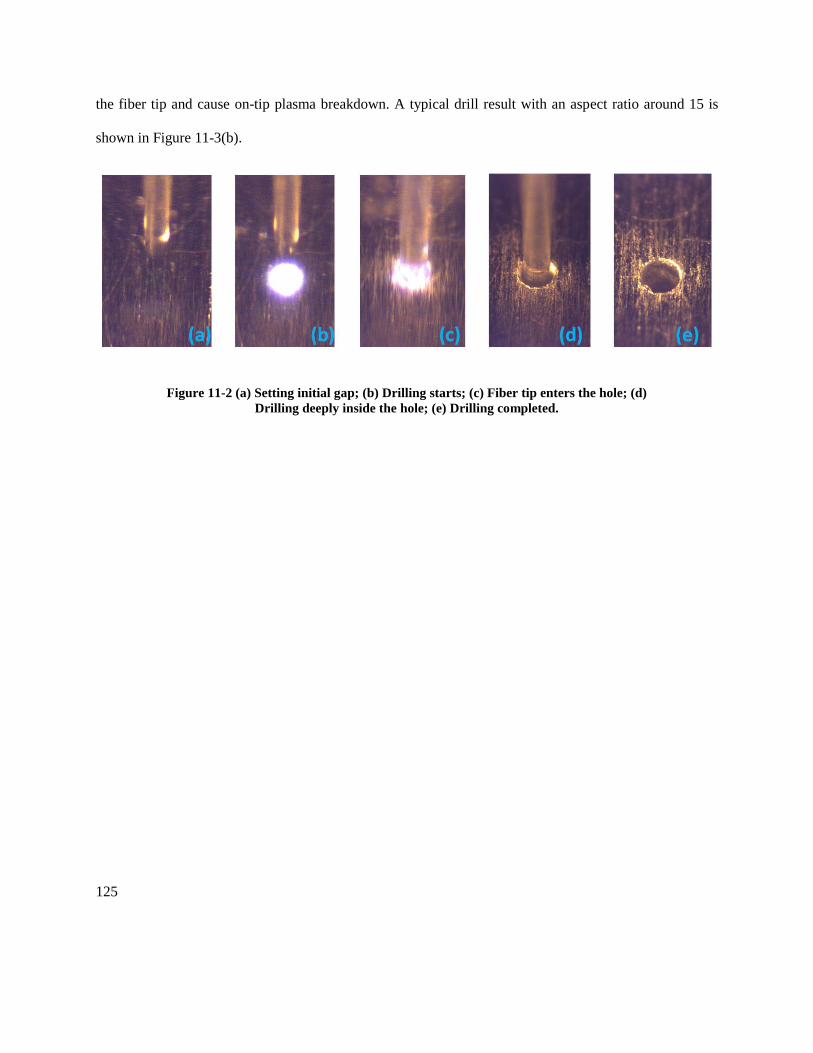
125
the fiber tip and cause on-tip plasma breakdown. A typical drill result with an aspect ratio around 15 is
shown in Figure 11-3(b).
Figure 11-2 (a) Setting initial gap; (b) Drilling starts; (c) Fiber tip enters the hole; (d)
Drilling deeply inside the hole; (e) Drilling completed.

126
Figure 11-3 Aluminum drilling results. (a) AR=8 hole with bare fiber for comparison; (b)
Fiber tip before and after the drilling process; (c) AR=15 hole; (d) AR=40 hole drilled on the
side wall.
To demonstrate that the GLMM method is capable of drilling even higher aspect-ratio hole with proper
debris removal, we performed a test on the side of an aluminum piece. In this test, we drilled on the very
edge of the aluminum piece and expose about ¼ of the hole for debris removing. To further avoid debris
forming on the fiber tip, a very low drilling speed (0.025 µm/pulse) was used. In this way, the fiber tip
was almost guaranteed to keep its distance from the drilling front. The plasma emission was collected by
the fiber tip and transmited back to the fiber input end surface. The end surface was monitored by an
imaging system and a CCD camera. In this way, the RGB channel value of the fiber core indicates the
intensity of the plasma emission. The following figure records the plasma emission intensity during the
drilling process described above. It can be seen that the plasma emission become weak before the tip

127
change and gain increased intensity after the tip change. This indicates the slow degradation of the fiber
tip which agrees with our post-process observation of the fiber tip.
Figure 11-4 The depth progression and LIP intensity record of the drilling process.
To verify that the debris is in the form of nano-particle, the debris was collected during the above drilling
process. The container that holds the aluminum sample was first thoroughly cleaned and DI water was
added in. Two silica cover slides were then put in the container near the to-be-drilled hole, one taken out
before the drilling started while the other one left in the container during the drilling process. After the
drilling competed, the cover slide that was contaminated by the drilling debris was taken out and dried in
a clean environment. The two cover slides were then observed under a Zygo surface profiler. There was
no debris found in the control group cover slide. Several measurements on the target cover slide were
performed and the debris was found to have a height (Sz) between 0.4um and 1.3um. Figure 11-5(a)
shows one typical result of these measurements. This has confirmed the assumption that the debris
generated during the process is in the nanometer range. Because of this, the debris should be able to exit
the side gap between the hole and the optical fiber if proper flushing mechanism were applied. Using the

128
surface profiler, the roughness of the drilled hole was also measured. As shown in Figure 11-5(b), the
surface roughness on the side wall of the drilled hole is about 2 µm.
Figure 11-5 (a) Drilling debris observation under surface profiler; (b) Side wall surface
roughness measurements by surface profiler.
Drilling results on PET
This fiber optics was also tested on PET as a demonstration of non-metallic material GLMM. A pulse
energy of 0.6 mJ and drilling speed of 0.2 µm/pulse was used in the tests. We were able to achieve
through holes with around 200 µm diameter on 25mm thick samples, giving an aspect ratio of 125. No
fiber tip change was performed during these processes. The results are shown in Figure 11-6. Due to the
heat sensitivity of the material and the long pulse width we used, a heat affected zone (surrounding semi-
black area) can be clearly observed. Based on our best knowledge, this is a record-setting aspect ratio for
non-tapered micro hole drilling on the plastic material. Additionally, this aspect ratio is not the limit for
even the current demonstrative setup, while the 25mm drilled depth is just the mechanical limitation of
the linear stage we used.

129
Figure 11-6 AR=125 PET drilling results
12 Conclusions to the fiber optic guided laser micromachining
A new method was introduced for laser micromachining, termed guided laser micromachining (GLMM).
Compared to the traditional free space laser beam machining, this method provides great potential in
achieving ultra-high aspect ratio. An ideal realization includes using special optical fiber with micro holes
for debris and bubble removing, which assist to achieve the highest possible aspect ratio. In this letter, we
have shown a simulation model to predict the relationship between drilling parameters and drilling results.
As a proof-of-concept, we have demonstrated the feasibility of this method by drilling on aluminum alloy
and PET with a standard multimode fiber. Due to the lack of fiber holes for debris and bubble removing,
the current system doesn’t reach the full capabilities of a proposed GLMM system. Nevertheless, a very
high aspect ratio of 40 was achieved on 7075 aluminum alloy and a record-setting aspect of 125 was
achieved on PET.
Based on these results, we are confident to predict that with a properly designed special optical fiber, this
GLMM should be able to achieve much higher aspect ratio compared to the currently existing laser beam
micromachining methods. More importantly, the potential of this GLMM method is not only limited to
straight micro hole drilling. With the optical fiber being flexible, this method is potentially capable of
curved hole drilling, with an external force applied to the fiber. An example is to coat the fiber tip with

130
magnetic materials and apply magnetic force during the drilling process. By varying the laser intensity
during the drilling process, micro holes with designed non-uniformity can be produced. And by moving
the fiber tip in the horizontal direction, high aspect ratio features instead of holes can be produced. We
believe the introduction of this new GLMM method opens a new sub-field under laser micromachining
with unique potentials and should be of interests to both researchers and industrial applications.

131
13 Dissertation summary
This dissertation presents two applications combining fiber optic and high power pulsed laser. In the first
application, a high temperature compatible structural health monitoring system was designed and
demonstrated. The result is a multiplexable monitoring system that can be attached at multiple points on a
large structure and provide information about the structural health at high temperature, which is crucial
for some high-value target such as power plants and aircraft engines. The key concept of the second
application is to use fiber guided high power laser beam to ablate materials, which enable very high
aspect ratio micromachining. The result is a demonstrative system that set new records in terms of aspect
ratio on both aluminum and PET.

132
Reference:
1. P. Castello, V. Guttmann, N. Farr, and G. Smith, "Laboratory‐simulated fuel‐ash corrosion of
superheater tubes in coal‐fired ultra‐supercritical‐boilers," Materials and Corrosion 51, 786-790
(2000).
2. B. Chorpening, D. Tucker, and S. Maley, "Sensors applications in 21st century fossil-fuel based power
generation," in Sensors, 2004. Proceedings of IEEE(IEEE, 2004), pp. 1153-1156.
3. S. M. Maley, and R. R. Romanosky, "Stakeholder Workshop. Advanced Process Control for Next
Generation Power Plants. Summary Report," Internet Citation,[Online] Jul 1, 78pp (2007).
4. V. Nagarkar, J. Gordon, S. Vasile, P. Gothoskar, and F. Hopkins, "High resolution X-ray sensor for
non-destructive evaluation," IEEE Trans. Nucl. Sci. 43, 1559-1563 (1996).
5. K. R. Leonard, E. V. Malyarenko, and M. K. Hinders, "Ultrasonic Lamb wave tomography," Inverse
problems 18, 1795 (2002).
6. H. Yan, H. Ning, Y. Kan, P. Wang, and M. J. Reece, "Piezoelectric Ceramics with Super‐High Curie
Points," J. Am. Ceram. Soc. 92, 2270-2275 (2009).
7. D. Van den Ende, W. Groen, and S. Van der Zwaag, "Development of temperature stable charge based
piezoelectric composite quasi-static pressure sensors," Sensors and Actuators A: Physical 163, 25-31
(2010).
8. R. Turner, P. A. Fuierer, R. Newnham, and T. Shrout, "Materials for high temperature acoustic and
vibration sensors: a review," Applied acoustics 41, 299-324 (1994).
9. H. Ning, H. Yan, and M. J. Reece, "Piezoelectric Strontium Niobate and Calcium Niobate Ceramics
with Super‐High Curie Points," J. Am. Ceram. Soc. 93, 1409-1413 (2010).
10. A. C. Tam, "Applications of photoacoustic sensing techniques," Rev. Mod. Phys. 58, 381-431 (1986).
11. V. Teslenko, "Investigation of photoacoustic and photohydrodynamic parameters of laser breakdown
in liquids," Soviet Journal of Quantum Electronics 7, 981 (1977).
12. X. Wu, Z. Duan, H. Song, Y. Wei, X. Wang, and C. Huang, "Shock pressure induced by glass-
confined laser shock peening: Experiments, modeling and simulation," J. Appl. Phys. 110, 053112-
053112-053117 (2011).
13. D. Devaux, R. Fabbro, L. Tollier, and E. Bartnicki, "Generation of shock waves by laser-induced
plasma in confined geometry," J. Appl. Phys. 74, 2268-2273 (1993).
14. F. Anabitarte, A. Cobo, and J. M. Lopez-Higuera, "Laser-induced breakdown spectroscopy:
fundamentals, applications, and challenges," ISRN Spectroscopy 2012 (2012).
15. M. D. Feit, and J. J. A. Fleck, "Light propagation in graded-index optical fibers," Appl. Opt. 17,
3990-3998 (1978).
16. W. Emkey, and C. Jack, "Analysis and evaluation of graded-index fiber lenses," Lightwave
Technology, Journal of 5, 1156-1164 (1987).
17. E. Desurvire, and J. R. Simpson, "Amplification of spontaneous emission in erbium-doped single-
mode fibers," Lightwave Technology, Journal of 7, 835-845 (1989).
18. P. M. Becker, A. A. Olsson, and J. R. Simpson, Erbium-doped fiber amplifiers: fundamentals and
technology (Academic press, 1999).
19. I. Pal, S. Sanghi, A. Agarwal, and M. Aggarwal, "Spectroscopic and structural investigations of Er<
sup> 3+</sup> doped zinc bismuth borate glasses," Materials Chemistry and Physics 133, 151-158
(2012).
20. C. R. Giles, and E. Desurvire, "Modeling erbium-doped fiber amplifiers," Lightwave Technology,
Journal of 9, 271-283 (1991).

133
21. S. J. Mihailov, D. Grobnic, C. W. Smelser, P. Lu, R. B. Walker, and H. Ding, "Induced Bragg
Gratings in Optical Fibers and Waveguides Using an Ultrafast Infrared Laser and a Phase Mask," Laser
Chemistry 2008, 1-20 (2008).
22. D. Grobnic, C. W. Smelser, S. J. Mihailov, and R. B. Walker, "Long-term thermal stability tests at
1000 °C of silica fibre Bragg gratings made with ultrafast laser radiation," Measurement Science and
Technology 17, 1009 (2006).
23. B. A. Auld, Acoustic fields and waves in solids (RE Krieger, 1990).
24. T. N. Bittencourt, P. A. Wawrzynek, A. R. Ingraffea, and J. L. Sousa, "Quasi-automatic simulation of
crack propagation for 2D LEFM problems," Engineering Fracture Mechanics 55, 321-334 (1996).
25. Z. Kala, "Sensitivity analysis of fatigue behaviour of steel structure under in-plane bending,"
Nonlinear Anal. Model. Control 11, 33-45 (2006).
26. R. L. Roderick, and R. Truell, "The Measurement of Ultrasonic Attenuation in Solids by the Pulse
Technique and Some Results in Steel," J. Appl. Phys. 23, 267-279 (1952).
27. E. P. Papadakis, "Ultrasonic Attenuation and Velocity in Three Transformation Products in Steel," J.
Appl. Phys. 35, 1474-1482 (1964).
28. A.-D. ANCAS, "Theoretical Models in the Study of Temperature Effect on Steel Mechanical
Properties."
29. C. EN, "1-2, Eurocode 3: design of steel structures, part 1.2: general rules—structural fire design,"
London: British Standards Institution (2005).
30. J. Skaar, "Modelling fiber bragg gratings," Cours de Institutt for elektronikk og telekommunikasjon
(2008).
31. A. D. McKie, J. W. Wagner, J. B. Spicer, and J. B. Deaton, "Dual-beam interferometer for the
accurate determination of surface-wave velocity," Appl. Opt. 30, 4034-4039 (1991).
32. G. Wild, and S. Hinckley, "Acousto-ultrasonic optical fiber sensors: Overview and state-of-the-art,"
IEEE Sens. J. 8, 1184-1193 (2008).
33. K. Vedam, "The elastic and photoelastic constants of fused quartz," Phys. Rev. 78, 472-473 (1950).
34. S.-C. Her, and C.-Y. Huang, "The effects of adhesive and bonding length on the strain transfer of
optical fiber sensors," Appl. Sci. 6, 13 (2016).
35. M. Weik, Fiber optics standard dictionary (Springer Science & Business Media, 2012).
36. M. V. Brook, Ultrasonic Inspection Technology Development and Search Unit Design: Examples of
Pratical Applications (John Wiley & Sons, 2012).
37. C. Diver, J. Atkinson, H. J. Helml, and L. Li, "Micro-EDM drilling of tapered holes for industrial
applications," J. Mater. Process. Technol. 149, 296-303 (2004).
38. C. Y. Yeo, S. C. Tam, S. Jana, and M. W. S. Lau, "A technical review of the laser drilling of
aerospace materials," J. Mater. Process. Technol. 42, 15-49 (1994).
39. K. P. Rajurkar, G. Levy, A. Malshe, M. M. Sundaram, J. McGeough, X. Hu, R. Resnick, and A.
DeSilva, "Micro and Nano Machining by Electro-Physical and Chemical Processes," CIRP Ann. Manuf.
Technol. 55, 643-666 (2006).
40. A. K. Dubey, and V. Yadava, "Laser beam machining—A review," Int. J. Mach. Tool. Manu. 48,
609-628 (2008).
41. H. Y. Zheng, and H. Huang, "Ultrasonic vibration-assisted femtosecond laser machining of
microholes," J. Micromech. Microeng. 17, N58 (2007).
42. M. K. Bhuyan, F. Courvoisier, P. A. Lacourt, M. Jacquot, L. Furfaro, M. J. Withford, and J. M.
Dudley, "High aspect ratio taper-free microchannel fabrication using femtosecond Bessel beams," Opt.
Express 18, 566-574 (2010).

134
43. J. Meijer, "Laser beam machining (LBM), state of the art and new opportunities," J. Mater. Process.
Technol. 149, 2-17 (2004).
44. A. P. Yalin, "High power fiber delivery for laser ignition applications," Opt. Express 21, A1102-
A1112 (2013).
45. L. M. Cabalín, and J. J. Laserna, "Experimental determination of laser induced breakdown thresholds
of metals under nanosecond Q-switched laser operation," Spectrochim. Acta B 53, 723-730 (1998).
46. J. Krüger, H. Niino, and A. Yabe, "Investigation of excimer laser ablation threshold of polymers
using a microphone," Appl. Surf. Sci. 197–198, 800-804 (2002).
47. J. M. Vadillo, and J. J. Laserna, "Laser-induced plasma spectrometry: truly a surface analytical tool,"
Spectrochim. Acta B 59, 147-161 (2004).
48. M. Capitelli, A. Casavola, G. Colonna, and A. De Giacomo, "Laser-induced plasma expansion:
theoretical and experimental aspects," Spectrochim. Acta B 59, 271-289 (2004).
49. B. J. Marquardt, S. R. Goode, and S. M. Angel, "In situ determination of lead in paint by laser-
induced breakdown spectroscopy using a fiber-optic probe," Anal. Chem. 68, 977-981 (1996).
50. G. W. Yang, "Laser ablation in liquids: Applications in the synthesis of nanocrystals," Prog. Mater.
Sci. 52, 648-698 (2007).
51. S. I. Dolgaev, A. V. Simakin, V. V. Voronov, G. A. Shafeev, and F. Bozon-Verduraz, "Nanoparticles
produced by laser ablation of solids in liquid environment," Appl. Surf. Sci. 186, 546-551 (2002).
52. T. Tsuji, K. Iryo, N. Watanabe, and M. Tsuji, "Preparation of silver nanoparticles by laser ablation in
solution: influence of laser wavelength on particle size," Appl. Surf. Sci. 202, 80-85 (2002).
53. B. N. Chichkov, C. Momma, S. Nolte, F. von Alvensleben, and A. Tünnermann, "Femtosecond,
picosecond and nanosecond laser ablation of solids," Appl. Phys. A 63, 109-115 (1996).
54. S. Fähler, and H.-U. Krebs, "Calculations and experiments of material removal and kinetic energy
during pulsed laser ablation of metals," Appl. Surf. Sci. 96–98, 61-65 (1996).
55. J. G. Lunney, and R. Jordan, "Pulsed laser ablation of metals," Appl. Surf. Sci. 127–129, 941-946
(1998).
56. P. R. Willmott, and J. R. Huber, "Pulsed laser vaporization and deposition," Rev. Mod. Phys. 72,
315-328 (2000).
57. D. Marla, U. V. Bhandarkar, and S. S. Joshi, "Modeling nanosecond pulsed laser ablation: A focus on
temperature dependence of material properties," Manufacturing Letters 2, 13-16 (2014).
58. M. Stafe, C. Negutu, A. N. Ducariu, and N. N. Puscas, "A spectroscopic and theoretical study of the
laser ablation rate of Al," (2012), pp. 841129-841129-841125.
59. A. Mele, A. Giardini Guidoni, R. Kelly, C. Flamini, and S. Orlando, "Laser ablation of metals:
Analysis of surface-heating and plume-expansion experiments," Appl. Surf. Sci. 109–110, 584-590
(1997).
60. J. R. Ho, C. P. Grigoropoulos, and J. A. C. Humphrey, "Computational study of heat transfer and gas
dynamics in the pulsed laser evaporation of metals," J. Appl. Phys. 78, 4696-4709 (1995).
61. S. H. Jeong, R. Greif, and R. E. Russo, "Numerical modeling of pulsed laser evaporation of
aluminum targets," Appl. Surf. Sci. 127–129, 177-183 (1998).
62. N. M. Bulgakova, A. V. Bulgakov, and L. P. Babich, "Energy balance of pulsed laser ablation:
thermal model revised," Appl. Phys. A 79, 1323-1326 (2004).