Two-dimensional sensitivity kernels for cross-correlation

functions of background surface waves

Kiwamu Nishida

Earthquake Research Institute, University of Tokyo, Tokyo, Japan

Abstract

Ambient noise tomography has now been applied at scales ranging from local

to global. To discuss the theoretical background of the technique, a simple

form of a two-dimensional (2-D) Born sensitivity kernel was developed at a

finite frequency for a cross-correlation function (CCF) of background sur-

face waves. The use of far field representations of a Green’s function and

a CCF in a spherically symmetric Earth model, assuming a homogeneous

source distribution, is an efficient approach to the calculation of phase sen-

sitivity kernels. The forms of a phase sensitivity kernel for major and minor

arc propagations are the same as those for phase-velocity measurements of

earthquake data. This result indicates the validity of ambient noise tomog-

raphy under the given assumptions; however, the kernels are not equivalent

in the case of an inhomogeneous source distribution.

Keywords: interferometry, sensitivity kernel, ambient noise tomography

1. Introduction

Shapiro et al. (2005) performed a cross-correlation analysis of long se-

quences of ambient seismic noise at around 0.1 Hz to obtain a group-velocity

anomaly of Rayleigh waves due to the lateral heterogeneity of the crust in

Preprint submitted to Comptes rendus Geoscience March 1, 2011

Southern California. The authors inverted the measured anomalies to obtain

a group-velocity map, employing a method that is now referred to as ‘am-

bient noise tomography‘. The obtained group–velocity map at short periods

(7.5–15 s) shows a striking correlation with the geologic structure.

Recently, phase velocity anomalies have also been measured using dense

networks of seismic stations (Bensen et al., 2007). The anomalies are inverted

to yield the three-dimensional S-wave velocity structure in the crust and

in the uppermost mantle (Nishida et al., 2008; Bensen et al., 2009). The

tomographic method was now been applied at scales ranging from local to

global (Nishida et al., 2009).

The theoretical basis of cross-correlation analysis is the fact that a cross-

correlation function (CCF) between a pair of stations provides the wave

propagation between them (Snieder, 2004), as with the Green’s function.

Assuming that a CCF has sensitivity along the ray path between a pair of

stations (Lin et al., 2009), the measured phase or group velocity anoma-

lies can be inverted to obtain maps of phase or group velocity. The ray

approximation is justified by the high-frequency limit of the phase–velocity

sensitivity kernel. The kernels for earthquake data have been evaluated by

many researchers (Spetzler et al., 2002; Yoshizawa and Kennett, 2005; Zhou

et al., 2004), but only one previous study has investigated ambient noise

tomography (Tromp et al., 2010).

In the present study, a form of a two-dimensional (2-D) Born sensitivity

kernel is obtained for a CCF, assuming the stochastic excitation of surface

waves. For simplicity, potential representation is used for surface waves. The

Born sensitivity kernel is then calculated in a spherically symmetric Earth

2

model assuming a homogeneous source distribution. A simple expression

of phase sensitivity kernels is derived from the Born sensitive kernel based

on the Rytov approximation with the far-field approximation of a Green’s

function and a CCF.

2. Theory of a synthetic cross spectrum of background surface

waves between a pair of stations

For estimation of the sensitivity kernels, this section develops the theory

of a synthetic CCF of background surface waves between a pair of stations.

It is assumed that a displacement field u can be represented by a funda-

mental Love wave and a fundamental Rayleigh wave, as follows:

u = uL + uR. (1)

Love and Rayleigh wave displacement fields in laterally, slowing varying me-

dia can be written in terms of surface wave potentials (Tanimoto, 1990;

Tromp and Dahlen, 1993). The Love wave part uL and the Rayleigh wave

part uR are given by the surface wave potential χα, as follows:

uα = Dαχα, (2)

where the subscript α represents the Love wave (L) or Rayleigh wave (R).

The spatial differential operators DR and DL are respectively defined as

follows:

DR = U(r, ω)r̂ + k−1R (r̂, ω)V (r, ω)∇l (3)

DL = k−1L (r̂, ω)W (r, ω)(−r̂ ×∇l), (4)

3

where ∇l is the surface gradient operator, U(r, ω) is the local vertical eigen-

function, ,V (r, ω) is the local radial eigenfunction, and W (r, ω) is the local

transverse eigenfunction as a function of surface location r, r̂ is a unit vector

defined on a unit sphere, and kα(r̂, ω) is the local wavenumber at the angu-

lar frequency ω. kα(r̂, ω) can also be written in terms of the phase velocity

cα(r̂, ω), as follows: kα(r̂, ω) = ω/cα(r̂, ω). The convention for the Fourier

transform is that exp(−iωt) appears in the Fourier integral when transform-

ing from the time domain to the frequency domain. The eigenfunctions are

normalized following Tromp and Dahlen (1993), as cα(r̂, ω)Cα(r̂, ω)I1α(r̂, ω) =

1, where Cα(r̂, ω) is the group velocity and I1α is the energy integral.

The surface wave potentials satisfy the inhomogeneous spherical Helmholtz

equation of a surface wave (Tromp and Dahlen, 1993), as follows:

∇2l χα(r̂, ω) + ξ2

α(r̂, ω)χα(r̂, ω) = Fα(r̂, ω), (5)

where ξα is the following complex wavenumber,

ξα(r̂, ω) = kα(r̂, ω) − ω

2Qα(r̂, ω)Cα(r̂, ω)i, (6)

where Qα is a quality factor. The equivalent surface traction Fα is defined

as follows:

FL(r̂, ω) = −kL(r̂, ω)W (r, ω)f3(r̂, ω)R2, (7)

FR(r̂, ω) = −(U(r, ω)f1(r̂, ω) + kR(r̂, ω)V (r, ω)f2(r̂, ω))R2, (8)

where R is the radius of the Earth. Here, f1 and f2 are spheroidal components

of the equivalent surface traction f , and f3 is a toroidal component of f in

the form of f = r̂f1 + ∇lf2 − r̂ ×∇lf3.

4

A scalar Green’s function of Love and Rayleigh waves Gα(r̂, r̂s, ω) satisfies

∇2l Gα(r̂, r̂s, ω) + ξ2

αGα(r̂, r̂s, ω) = −δ(r̂, r̂s). (9)

A scalar potential function χα can be written as

χα(r̂, ω) =

∫Σ

Gα(r̂, r̂s, ω)Fα(r̂s, ω)dΣ, (10)

where Σ is the unit sphere.

The cross spectrum Φ of background surface waves between stations r1

and r2 can be given by

Φ(r1, r2, ω) = 〈u(r1, ω)u∗(r2, ω)〉

= D1LD2

LΦLL(r̂1, r̂2, ω) + D1RD2

RΦRR(r̂1, r̂2, ω)

+ D1LD2

RΦLR(r̂1, r̂2, ω) + D1RD2

LΦRL(r̂1, r̂2, ω) (11)

where ∗ represents a complex conjugate, 〈〉 denotes an ensemble (statis-

tical) average, an αβ component of the cross spectrum Φαβ(r̂1, r̂2, ω) is⟨χα(r̂1, ω)χ∗

β(r̂2, ω)⟩, and Di

α is the spatial derivative at point r̂i. For sim-

plicity, the αβ component of the cross spectrum Φαβ(r̂1, r̂2, ω) is evaluated

below.

The cross spectrum Φαβ(r̂1, r̂2, ω) can be written as follows:

Φαβ(r̂1, r̂2, ω) =

∫Σ

∫Σ

Gα(r̂1, r̂, ω)G∗β(r̂2, r̂

′, ω)Ψαβ(r̂, r̂′, ω)dΣdΣ′, (12)

where Ψαβ is the cross spectrum of surface traction⟨Fα(r̂, ω)F ∗

β (r̂′, ω)⟩

be-

tween points r̂ and r̂′. Assuming that the excitation sources of the back-

ground surface waves are spatially isotropic but heterogeneous, the cross

spectrum Ψαβ(r̂′, r̂′′, ω) is expressed in the following form:

Ψαβ(r̂′, r̂′′, ω) =

√Ψ̂αβ(r̂′, ω)Ψ̂αβ(r̂′′, ω)h

(1 − | r̂′ − r̂′′ |

L(r̂′, ω)

), (13)

5

where Ψ̂αβ(r, ω) is a power spectrum of surface traction at r̂ (Fukao et al.,

2002; Nishida and Fukao, 2007), L(r̂′, ω) is the frequency-dependent coherent

length, and the function h(x) is the Heviside step function.

The excitation mechanism of ambient noise from 0.05 to 0.2 Hz, known as

microseisms, is firmly established. Microseisms are identified at the primary

and double frequencies: the primary microseisms at around 0.08 Hz have been

ascribed to the direct loading of ocean swell onto a sloping beach (Haubrich

et al., 1963). The typical frequency of secondary microseisms at around 0.15

Hz is approximately double the typical frequency of ocean swells, indicating

the generation of the former via nonlinear wave–wave interactions among the

latter (Longuet-Higgens, 1950). In both cases of the excitation mechanisms,

the correlation length L can be characterized by the wavelength of ocean

swell, on the order of 300 m, which is expected to be much shorter than the

wavelength of seismic surface waves.

Supposing that the correlation length L(ω) is much shorter than the typ-

ical wavelength of background surface waves at ω, the cross spectrum Φαβ

can be simplified as follows:

Φαβ(r̂1, r̂2, ω) = 4π2

∫Σ

Ψ̂eαβ(r̂, ω)Gα(r̂1, r̂)G∗

β(r̂2, r̂)dΣ. (14)

Here, the power spectrum of effective surface traction per unit wavenumber

Ψ̂eαβ(ω) is defined as follows:

Ψ̂eαβ(r̂, ω) ≡ L2(r̂, ω)

4πR2Ψ̂αβ(r̂, ω). (15)

6

3. 2-D Born sensitivity kernel for a CCF of background surface

waves in the case of a heterogeneous source distribution

Employing a first-order Born approximation of a cross spectrum Φαβ (eq.

14), a 2-D Born sensitivity kernel is estimated for the cross spectrum, which

is a representation of a CCF in the frequency domain.

The first-order perturbation of the cross spectrum δΦ can be written in

terms of the perturbation of the Green’s function δG, as follows:

δΦαβ(r̂1, r̂2, ω) = 4π2

∫Σ

Ψ̂eαβ(r̂, ω)

{δGα(r̂1, r̂, ω)G∗

β(r̂2, r̂, ω)

+ Gα(r̂1, r̂, ω)δG∗β(r̂2, r̂, ω)

}dΣ.(16)

δGα can be written as follows (e.g. Yoshizawa and Kennett, 2005):

δGα(r̂1, r̂, ω) =

∫Σ

−2k2α(r̂3, ω)

δc(r̂3, ω)

c(r̂3, ω)Gα(r̂1, r̂3)Gα(r̂3, r̂)dΣ3. (17)

The above equation can then be simplified as follows:

δΦαβ(r̂1, r̂2, ω) =

∫Σ

Kαβ(r̂1, r̂2, r̂3, ω)δc(r̂3, ω)

c(r̂3, ω)dΣ3. (18)

A 2-D Born sensitivity kernel for phase–velocity anomalies is defined as fol-

lows:

Kαβ(r̂1, r̂2, r̂3, ω) =

−2{k2

αΦ∗βα(r̂2, r̂3, ω)Gα(r̂1, r̂3) + k2

βΦαβ(r̂1, r̂3, ω)G∗β(r̂2, r̂3)

}.(19)

This form of the above equation is similar to that of an adjoint kernel

(e.g. Tarantola, 1984; Tanimoto, 1990; Tromp et al., 2010). For example, the

first term of the kernel can be represented by convolution in the time domain

between the time reversal of the CCF and the propagating Green’s function

from r̂2 to r̂3.

7

4. 2-D Born sensitivity kernel in a spherically symmetric Earth

model for a homogeneous source distribution

For simplicity, the focus is on 2-D Born sensitivity kernels in a spherically

symmetric Earth model for a homogeneous source distribution. A scalar

Green’s function in a homogeneous model can be simplified in the following

form:

Gα(r̂1, r̂2, ω) =∑

l

(2l + 1

4π(ξ2α − l(l + 1))

)Pl(cos Θ12), (20)

where Θ12 is the angular distance between r̂1 and r̂2, and Pl is the Legendre

function of the l’th order.

In this section, it is assumed that homogeneous and isotropic sources

excite background surface waves. This approximation enables us to simplify

the α component of a cross spectrum in the following form:

Φαα(r̂1, r̂2, ω) = Ψ̂eαα(ω)π

∑l

2l + 1

(ξ2α − l(l + 1))(ξ∗2α − l(l + 1))

Pl(cos Θ12).

(21)

The cross terms Φαβ are omitted for α 6= β because they take values of zero

in the case of a homogeneous source distribution.

Figure 1 shows a typical example of the Born sensitivity kernel of a

Rayleigh wave at 5.61 mHz with the source spectrum Ψeαα of an empirical

model (Fukao et al., 2002). The sensitivity is concentrated within the first

Fresnel zone. The figure also shows the side lobes of the kernel, which are

suppressed when considering band-limited kernels (Yoshizawa and Kennett,

2005), as shown in the following section.

To obtain a more comprehensive form of the kernel, a far-field approxi-

mation of the Green’s function and the CCF is considered. A far-field repre-

8

sentation of Green’s function is given as follows (Tromp and Dahlen, 1993):

Gα(r̂1, r̂2, ω) =∞∑

s=1

gsα(∆s

12, ω). (22)

The Green’s function of the s’th orbit gsα is defined as follows:

gsα(∆s

12, ω) =ei(−kα∆s

12+(s−1)π2−π

4 )e−ω∆s

122CαQα√

8πkα sin | ∆s12 |

, (23)

where the integer s(= 1, 2, · · · ) represents the surface wave orbits. The quan-

tity ∆s12, which is the total angular distance traversed by a given arrival, is

given by explicitly by,

∆s12 =

Θ12 + (s − 1)π, s odd

sπ − Θ12, s even.

(24)

Similarly to the approximation of the Green’s function (Dahlen and Tromp,

1998, chapter 11.1), a far-field representation of the CCF is evaluated. Us-

ing the Poisson sum formula (Dahlen and Tromp, 1998, eq. 11.4, p. 408)

to convert the summation over the angular degree l to an integral over the

wavenumber k, the following representation is obtained:

Φαα(r̂1, r̂2, ω) = Ψ̂eαα(ω)π

∞∑s=−∞

(−1)s

∫ ∞

0

2

(ξ2α − k2)(ξ∗2α − k2)

Pk− 12e−2iskπkdk.

(25)

The above equation is transformed into a traveling representation of the

CCF (Dahlen and Tromp, 1998, chapter 11.2), as follows:

Φαα(r̂1, r̂2, ω) = 2Ψ̂eαα(ω)π

[∞∑

s=1,3,···

(−1)(s−1)/2

∫ ∞

−∞

Q(1)k−1/2e

−i(s−1)kπ

(ξ2α − k2)(ξ∗2α − k2)

kdk

∞∑s=2,4,···

(−1)s/2

∫ ∞

−∞

Q(2)k−1/2e

−iskπ

(ξ2α − k2)(ξ∗2α − k2)

kdk

].(26)

9

The analysis employs a relation of the transformation into a traveling

wave representation (Dahlen and Tromp, 1998, appendix B.11), as follows:

Pk− 12(cos Θ) = Q

(1)

k− 12

(cos Θ) + Q(2)

k− 12

(cos Θ), (27)

where Q(1,2)k−1/2 corresponds to waves propagating in the direction of increasing

and decreasing Θ, respectively. The following equation is also employed

(Dahlen and Tromp, 1998, eq. 11.13):

Q(1,2)

−k− 12

(cos Θ) = e±2ikπQ(1,2)

k− 12

(cos Θ) + e±ikπ tan kπPk− 12(− cos Θ). (28)

Following Dahlen and Tromp (1998, chapter 11.3), the far-field approxi-

mation of the CCF is obtained as follows:

Φαα(r̂1, r̂2, ω) =∞∑

s=1

φsα, (∆s

12, ω), (29)

where φsα(∆s

12, ω) is the cross spectrum of the s’th orbit, as follows:

φsα(∆s

12, ω) = Ψ̂eαα(ω)

2π2QαCα

ω

{gs

α(∆s12, ω)e

π2

i + gs∗α (∆s

12, ω)e−π2i}

. (30)

Because the cross spectrum Φαα(Θ12, ω) is a real function, the correspond-

ing CCF is an even function, which has a causal part and an acausal part.

The first term represents the causal part of the cross spectrum; the second

term represents the acausal part. This equation shows the phase retreat

(π/2) of the causal part of the corresponding CCF from the Green’s function

(Nakahara, 2006; Sanchez-Sesma and Campillo, 2006).

The symmetry between the causal and acausal parts is broken in the case

of heterogeneous distribution of sources (Cupillard and Capdeville, 2010;

Kimman and Trampert, 2010; Nishida and Fukao, 2007). Source heterogene-

ity also causes a bias of the phase from 0 to π/4 (Kimman and Trampert,

2010).

10

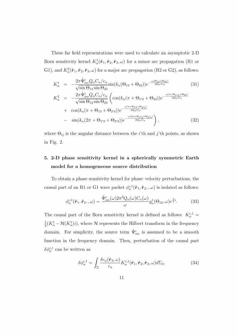
These far field representations were used to calculate an asymptotic 2-D

Born sensitivity kernel K1α(r̂1, r̂2, r̂3, ω) for a minor arc propagation (R1 or

G1), and K2α(r̂1, r̂2, r̂3, ω) for a major arc propagation (R2 or G2), as follows:

K1α = −2πΨ̂e

ααQαCα/cα√sin Θ13 sin Θ23

sin(kα(Θ13 + Θ23))e−ω(Θ13+Θ23)

2QαCα (31)

K2α = −2πΨ̂e

ααQαCα/cα√sin Θ13 sin Θ23

(cos(kα(π + Θ1′3 + Θ23))e

−ω(π+Θ1′3+Θ23)

2QαCα

+ cos(kα(π + Θ13 + Θ2′3))e−

ω(π+Θ13+Θ2′3)

2QαCα

− sin(kα(2π + Θ1′3 + Θ2′3))e−

ω(2π+Θ1′3+Θ2′3)

2QαCα

), (32)

where Θij is the angular distance between the i’th and j’th points, as shown

in Fig. 2.

5. 2-D phase sensitivity kernel in a spherically symmetric Earth

model for a homogeneous source distribution

To obtain a phase sensitivity kernel for phase–velocity perturbations, the

causal part of an R1 or G1 wave packet φc,1α (r̂1, r̂2, , ω) is isolated as follows:

φc,1α (r̂1, r̂2, , ω) =

Ψ̂eαα(ω)2π2Qα(ω)Cα(ω)

ωg1

α(Θ12, ω)eπ2i. (33)

The causal part of the Born sensitivity kernel is defined as follows: Kc,1α =

12(K1

α −H(K1α)i), where H represents the Hilbert transform in the frequency

domain. For simplicity, the source term Ψ̂eαα is assumed to be a smooth

function in the frequency domain. Then, perturbation of the causal part

δφc,1α can be written as

δφc,1α =

∫Σ

δcα(r̂3, ω)

cα

Kc,1α (r̂1, r̂2, r̂3, ω)dΣ3. (34)

11

The Rytov approximation is employed to obtain a phase sensitivity kernel

for phase–velocity perturbations (e.g. Yoshizawa and Kennett, 2005; Zhou et

al., 2004). In the Rytov method, the logarithm of the cross spectrum φc,1α is

considered instead of the wavefield itself. By taking the logarithm, φc,1α can

be divided into real (amplitude) and imaginary (phase) parts, as follows:

ln φc,1α = ln(A1

α exp(−ψ1αi)) = ln A1

α − ψ1αi, (35)

where A1α is the amplitude of the causal wave packet, and ψ1

α is its phase.

The phase perturbation δψ1α for propagation along the minor arc (R1 or G1)

is given by

δψ1α =

∫K1

p,α(r̂1, r̂2, r̂3, ω)δc

cdΣ3, (36)

where the phase sensitivity kernel K1p,α is the imaginary part of −Kc,1

α /φc,1α .

Using the asymptotic kernel Kc,1α , a phase sensitivity kernel for R1 or G1

can be written as

K1p,α = − k

32α√2π

(sin Θ12

sin Θ13 sin Θ23

) 12

cos(kα(Θ13 + Θ23 − Θ12) −

π

4

)e−

ω(Θ13+Θ23−Θ12)2QαCα .

(37)

This expression of the phase sensitivity kernel is the same as that for phase

measurements of earthquake data (Yoshizawa and Kennett, 2005). The

equivalence of the expressions serves as validation of ambient noise tomog-

raphy. Of course, this discussion is valid only under the assumptions of

one-dimensional background structure and a homogeneous source distribu-

tion.

Actual phase-velocity anomalies are measured with a finite frequency

band (e.g. Bensen et al., 2007). To consider a sensitivity kernel for phase

measurements, an averaged phase-velocity kernel K̄1p,α in a certain frequency

12

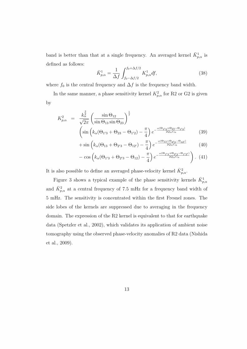
band is better than that at a single frequency. An averaged kernel K̄1p,α is

defined as follows:

K̄1p,α =

1

∆f

∫ f0+∆f/2

f0−∆f/2

K1p,αdf, (38)

where f0 is the central frequency and ∆f is the frequency band width.

In the same manner, a phase sensitivity kernel K2p,α for R2 or G2 is given

by

K2p,α =

k32α√2π

(sin Θ12

sin Θ13 sin Θ23

) 12

(sin

(kα(Θ1′3 + Θ23 − Θ1′2) −

π

4

)e−

ω(Θ1′3+Θ23−Θ1′2)

2QαCα (39)

+ sin(kα(Θ13 + Θ2′3 − Θ12′) −

π

4

)e−

ω(Θ13+Θ2′3−Θ12′ )2QαCα (40)

− cos(kα(Θ1′3 + Θ2′3 − Θ12) −

π

4

)e−

ω(Θ1′3+Θ2′3−Θ1′2′ )2QαCα

). (41)

It is also possible to define an averaged phase-velocity kernel K̄2p,α.

Figure 3 shows a typical example of the phase sensitivity kernels K̄1p,α

and K̄2p,α at a central frequency of 7.5 mHz for a frequency band width of

5 mHz. The sensitivity is concentrated within the first Fresnel zones. The

side lobes of the kernels are suppressed due to averaging in the frequency

domain. The expression of the R2 kernel is equivalent to that for earthquake

data (Spetzler et al., 2002), which validates its application of ambient noise

tomography using the observed phase-velocity anomalies of R2 data (Nishida

et al., 2009).

13

6. Effects of heterogeneous distribution of sources on a Born sen-

sitivity kernel

This section considers the effects of heterogeneous distribution of sources

on the Born sensitivity kernel. For simplicity, the kernel K1α is considered in

a spherically symmetric case for the minor arc. It is simply assumed, phe-

nomenologically, that the cross spectrum φ1α has only azimuthal dependency,

as follows:

φ1α(∆1

12, ω) = Ψ̂eαα

2π2QαCα

ω

(a(ϕ12)g

1α(∆1

12, ω)e12πi + a(ϕ21)g

1∗α (∆1

12, ω)e−12πi

),

(42)

where a(ϕ) is a real coefficient that varies as a function of azimuth, and ϕ12

is the back-azimuth to r̂2 at r̂1. Because the focus is on the perturbation of

a time-symmetric part of a CCF, the real part of the Born sensitivity kernel

K1α is evaluated, as follows:

<[K1α] ∝ −{a(ϕ23) + a(ϕ13)} sin(kα(Θ23 + Θ13))

−{a(ϕ23) − a(ϕ13)} cos(kα(Θ23 − Θ13)), (43)

where < indicates the real part. The first term shows an elliptic pattern with

foci at the stations, whereas the second term shows a hyperbolic pattern with

foci at the stations. The second term vanishes in the case of a homogeneous

source distribution, as in eq. 31. If the time symmetry of the CCF is broken

because of a heterogeneous source distribution, the second term would take

on a hyperbolic pattern. Thus, the antisymmetry causes a bias in phase

velocity maps, even without phase changes in the causal and acausal parts.

Note that the second term vanishes in the case of | r̂3 |À| r̂2 − r̂1 |.

14

Of course, the coefficient a(ϕ) may have a imaginary part because an

incomplete source distribution also causes a bias in the phase from 0 to π/4

(Kimman and Trampert, 2010). The imaginary part also causes a severe bias

of the Born sensitivity kernel.

7. Conclusion

A theory of Born and phase sensitivity kernels was developed for a CCF

using potential representation for surface waves. Simple forms were shown of

Born and phase sensitivity kernels of a CCF in a spherically symmetric Earth

model, assuming a homogeneous source distribution. The expression of the

resultant phase sensitivity kernel is equivalent to that for phase measure-

ments of earthquake data. This equivalence indicates the validity of ambient

noise tomography under the given assumptions. The incomplete source dis-

tribution defines a hyperbolic pattern with foci at the pair of stations in a

spherically symmetric case, which would generate a bias in the measured

phase-velocity anomaly.

Acknowledgment

The author thanks Dr. Anne Seiminski, an anonymous reviewer, and the

associate editor Dr. Michel Campillo for their constructive comments.

15

References

Bensen, G.D., Ritzwoller, M.H., Barmin, M.P., Levshin, A.L., Lin, F.,

Moschetti, M.P. Shapiro, N.M., Yang, Y., Processing seismic ambient noise

data to obtain reliable broad-band surface wave dispersion measurements,

2007, Geophys. J. Int., 169, 1239-1260.

Bensen, G.D., Ritzwoller, M.H., Yang, Y., A 3D shear velocity model of

the crust and uppermost mantle beneath the United States from ambient

seismic noise, 2009, Geophys. J. Int.,177, 1177-1196.

Cupillard, P., Capdeville, Y., On the amplitude of surface waves obtained by

noise correlation and the capability to recover the attenuation: a numerical

approach, 2010, Geophys. J. Int., 181, 1687–1700.

Dahlen, F.A., Tromp, J. 1998. Theoretical Global Seismology, Princeton Uni-

versity Press, NJ, USA, 1025 p.

Dziewonski, A.M., Anderson, D.L., Preliminary reference Earth model., 1981,

Phys. Earth. Planet. Inter., 25, 97-356.

Fukao, Y., Nishida, K., Suda, N., Nawa, K., Kobayashi, N., 2002, A theory of

the Earth’s background free oscillations, J. Geophys. Res., 107, B9, 2206.

Haubrich, R., Munk, W., Snodgrass, F.. 1963, Comparative spectra of mi-

croseisms and swell, Bull. Seismol. Soc. Am., 53, 27-37.

Kimman, W.P., Trampert, K., Approximations in seismic interferometry and

their effects on surface waves, 2010, Geophys. J. Int. 182, 461–476.

16

Lin, F.C., Ritzwoller, M.H., Snieder, R., 2009, Eikonal Tomography: Surface

wave tomography by phase-front tracking across a regional broad-band

seismic array. Geophys. J. Int., 177, 1091-1110.

Longuet-Higgens, M.S., 1950, A theory of the origin of microseisms, Phil.

Trans. of the Roy. Soc. of London, 243, 1-35.

Nakahara, H., A systematic study of theoretical relations between spatial

correlation and Green’s function in 1D, 2D and 3D random scalar wave

fields, 2006, Geophys. J. Int., 167, 1097-1105.

Nishida, K., Fukao, Y., Source distribution of Earth’s background free oscil-

lations, 2007, J. Geophys. Res., 112, B06306.

Nishida, K., Kawakatsu, H., Obara, K., Three-dimensional crustal S-wave

velocity structure in Japan using microseismic data recorded by Hi-net

tiltmeters, 2008, J. Gephys. Res., 113, B10302.

Nishida, K., J.P. Montagner, Kawakatsu, H., 2009, Global Surface Wave

Tomography Using Seismic Hum, Science, 326, 112.

Sanchez-Sesma, F.J., Campillo, M., Retreival of the Green function from

cross-correlation: the canonical elastic problem, 2006, Bull. Seismol.

Soc.Am., 96, 1182–1191.

Shapiro N., Campillo, M., Stehly, L., Ritzwoller, M., High-Resolution

Surface-Wave Tomography from Ambient Seismic Noise, 2005, Science,

307, 1615-1618.

17

Snieder, R., Extracting the Green’s function from the correlation of coda

waves: A derivation based on stationary phase, 2004, Phys. Rev. E, 69,

046610.

Spetzler, J., J. Trampert, Snieder, R., The effect of scattering in surface wave

tomography, 2002, Geophys. J. Int., 149, 755-767.

Tanimoto, T., 1990, Modelling curved surface wave paths; membrane surface

wave synthetics, Geophys. J. Int., 102, 89–100.

Tarantola.. A., Inversion of seismic reflection data in the acoustic approxi-

mation, 1984, Geophysics, 49, 1259–1266.

Tromp, J., Dahlen, F.A., Variational principles for surface wave propaga-

tion on a laterally heterogeneous Earth–III, Potential representation, 1993,

Geophys. I. Int., 112, 195-209.

Tromp, J., Luo, Y., Hanasoge, S., Peter, D., Noise cross-correlation sensitiv-

ity kernels, 2010, Geophys. J. Int., 183, 791–819.

Yoshizawa, K., Kennett, B.L.N., 2005, Sensitivity kernels for finite-frequency

surface waves, Geophys. J. Int., 162, 910–926.

Zhou, Y. Dahlen, F.A., Nolet, G., 2004, Three-dimensional sensitivity kernels

for surface wave observables. Geophys. J. Int., 158, 142–168.

18

Figure 1: Born sensitivity kernel of a Rayleigh wave at 5.61 mHz, with amplitude nor-

malized by the cross spectrum Φαα(Θ12, ω). Each station is located on the equator. The

longitude of station 1 is 40◦; that of station 2 is 140◦. The kernel was calculated using

PREM (Dziewonski and Anderson, 1981). S1, S2, A1, and A2 indicate the locations of

station 1, station 2, the antipode of station 1, and the antipode of station 2, respectively.

This kernel is not singular, even near stations and near the antipodes of the stations.

Figure 2: Schematic map of the geometry of stations and their antipodes. Star symbols

show the locations of stations at r̂2 and r̂2, and those of their antipodes at r̂′1 and r̂′

2.

The open circle shows the location of a phase velocity anomaly at r̂3.

Figure 3: Imaginary part of the Rytov sensitivity kernels (K̄1p,α and K̄2

p,α) of the fun-

damental Rayleigh wave at a central frequency of 7.5 mHz (from 5 to 10 mHz). Each

station is located on the equator. The lower panel and the left-hand panel show slices of

the kernels along the paths indicated by solid lines (an equatorial path, and the lines of

longitude at 90◦ and 140◦). The lower panel shows that the kernels have negative values

along the minor and major arcs.

19

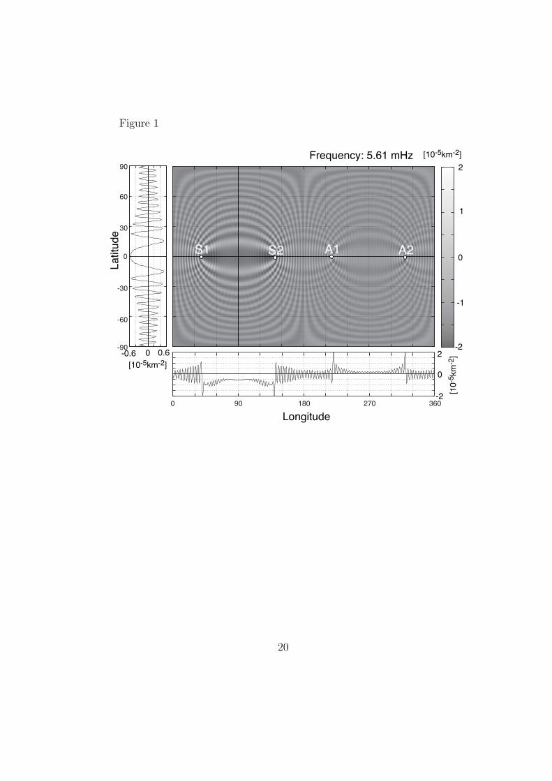
Figure 1

-90

-60

-30

0

30

60

90

0 90 180 270 360

2

-2

-1

1

0

2

0

[10-5km-2]

-2

0-0.6

Longitude

[10-5km-2]

[10

-5km

-2]

La

titu

de

0.6

S1 S2 A1 A2

Frequency: 5.61 mHz

20

Figure 2

r1 r2

r3

Station 1 Station 2

Θ12

Θ13Θ23

r1’ r2’

Antipode of station 1

Antipode of station 2

Θ1’3 Θ2’3

Θ1’2^ ^

^

^ ^Θ1’2’

21

Figure 3

-90

-60

-30

0

30

60

90

0 90 180 270 360

-1

1

0

2

0

[10-5km-2]

-4

0-1

Longitude

[10-5km-2]

[10

-5km

-2]

La

titu

de

Central Frequency: 7.5 mHz (5-10 mHz)

lon

=9

0lo

n=

27

0

K2K1

K1

K2

-2 p,R

p,R

p,R

p,R

22