Two-dimensional Array Beam Scanning

via Externally and Mutually Injection Locked Coupled Oscillators

Ronald J. Pogorzelski

Jet Propulsion Laboratory

California Institute of TechnologyPasadena. CA 91 ! 09

Background

Some years ago, Stephan [1] proposed an approach to one dimensional (linear) phased array beam steering

which requires only a single phase shifter. This involves the use of a linear array of voltage-controlled

electronic oscillators coupled to nearest neighbors. The oscillators are mutually injection locked by

controlling their coupling and tuning appropriately.J2][3] Stephan's approach consists of deriving two

signals from a master oscillator, one signal phase shifted with respect to the other by means of a single

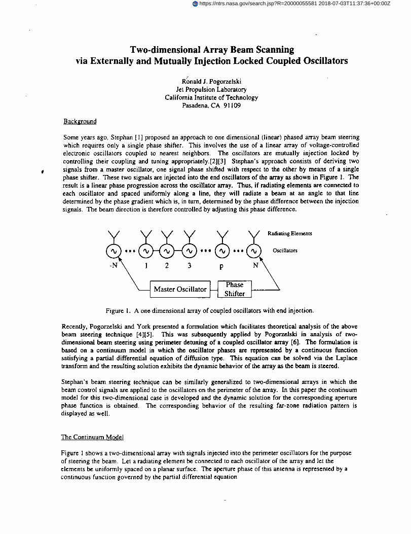
phase shifter. These two signals are injected into the end oscillators of the array as shown in Figure 1. The

result is a linear phase progression across the oscillator array. Thus, if radiating elements are connected to

each oscillator and spaced uniformly along a line, they will radiate a beam at an angle to that linedetermined by the phase gradient which is, in turn, determined by the phase difference between the injection

signals. The beam direction is therefore controlled by adjusting this phase difference.

_ , _ _ _ RadiatingElernents

-N _ 11 2 3 p N

Master Oscillator sPhiftaSeer 1

Figure 1. A one dimensional array of coupled oscillators with end injection.

Recently, Pogorzelski and York presented a formulation which facilitates theoretical analysis of the above

beam steering technique [4][5]. This was subsequently applied by Pogorzelski in analysis of two-dimensional beam steering using perimeter detuning of a coupled oscillator array [6]. The formulation is

based on a continuum model in which the oscillator phases are represented by a continuous functionsatisfying a partial differential equation of diffusion type. This equation can be solved via the Laplace

transform and the resulting solution exhibits the dynamic behavior of the array as the beam is steered.

Stephan's beam steering technique can be similarly generalized to two-dimensional arrays in which the

beam control signals are applied to the oscillators on the perimeter of the array. In this paper the continuum

model for this two-dimensional case is developed and the dynamic solution for the corresponding aperturephase function is obtained. The corresponding behavior of the resulting far-zone radiation pattern is

displayed as well.

The Continuum Model

Figure I shows a two-dimensional array with signals injected into the perimeter oscillators for the purposeof steering the beam. Let a radiating element be connected to each oscillator of the array and let the

elements be uniformly spaced on a planar surface. The aperture phase of this antenna is represented by a

continuous function governed by the partial differential equation

https://ntrs.nasa.gov/search.jsp?R=20000055581 2018-07-03T11:37:36+00:00Z

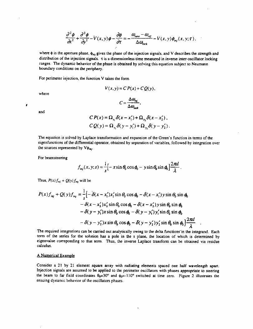
d 2 . d 2# de - w,,Io3x2 + o3y2 - V (x , Y )¢) - _ =_- A cotoa V (x, y)O,.j (x, y; r ),

where $ is the aperture phase, $i.j gives the phase of the injection signals, and V describes the strength and

distribution of the injection signals. %is a dimensionless time measured in inverse inter-oscillator locking

ranges. The dynamic behavior oftbe phase is obtained by solving this equation subject to Neumannboundary conditions on the periphery.

For perimeter injection, the function V takes the form

where

and

V (x, y) = C P(x)+ C Q(y),

C- A_"i)

c P(x)= - x:)+ 6(x-

CQ(y) = _:.,8(y- yf)+ny S(y- y_).

The equation is solved by Laplace transformation and expansion of the Green's function in terms of theeigenfunctions of the differential operator, obtained by separation of variables, followed by integration overthe sources represented by V_i.j.

For beamsteering

1fi.j(x,y;S)=s[- xsin O0cosCb- ysinO0sin ¢b] 2_rd "

Thus, P(x) f.j + Q(y) f.j will be

1_

P(x)fi.j + Q(Y)fi.j _[ " " " "= -6(x-xl)x 1sm0ocos0 o-8(x-x;)ysin0osin0 o

- 8(x - x_ )x_ sin 0o cos 0o - 6(x - x_)y sin 0o sin 0o

- 8(y - y[)x sin 0o cos0o - 8(y - y[)y[sin 0o sin 0o

2trd

- 8(y- y_)xsin Oo cOS0o - 8(y- y_)y_ sin Oosin ¢o ] -_

The required integrations can be carried out analytically owing to the delta functions'in the integrand. Eachterm of the series for the solution has a pole in the s plane, the location of which is determined byeigenvalue correponding to that term. Thus, the inverse Laplace transform can be obtained via residuecalculus.

A Numerical Example

Consider a 21 by 21 element square array with radiating elements spaced one half wavelength apart.Injection signals are assumed to be applied to the perimeter oscillators with phases appropriate to steeringthe beam to far field coordinates 80=30 ° and _bo=-II0* switched at time zero. Figure 2 illustrates theensuing dynamic behavior of the oscillators phases.

Oscillator Phases

Two O_n_r_onQl An'11y

e. 3oae_ms

l-.11o _gmes

I I! , !

Figure 2. Phase dynamics during beam steering.

Note that during this transient period the phase surface is nonplanar which results in some aberrationinduced gain reduction and sideiobe distortion in the far-zone beam. Figure 3 shows the effect of this

aberration on the far-zone gain as a function of time• The curve labeled "Ideal Gain" includes the projectedaperture loss but no aberration loss for comparison.

34

32

3O

.-o.

24

P9

200

• • II_lmm

"_" *. -_le

10 20 30 40 50

Time [Inver_-r_e LocWJng Flanges]

Figure 3. Antenna gain during beam steering.

Finally, Figure 4 shows the result of successive application of a sequence of beamsteering by displaying thelocations of the beam peak and the three dB contour at a sequence of times and the effect of aberration onthe beam shape is evident•

30Beam Traiectory

Penmeler _leclmon

20 " '

C3 0c"

_:_ -10<_

-20

J _ _njaaa_ (C-O.D-30 ............. ...... !,c_.._....-30 -20 -10 0 10 20 30

Angle in Degrees

Figure 4. Sequential beam steering.

Acknowledgment

The research descr/bed in this paper was performed by the Center for Space Microelectronics Technology,Jet Propulsion Laboratory, California Institute of Technology, and was sponsored by the BaUistic Missile

Defense Organization through an agreement with the National Aeronautics and Space Administration.

Reference8

1. K. D. Stephan, "Inter-Injection-Locked Oscillators for Power Combining and Phased Arrays," IEEETrans. Microwave Theory and Tech., MTT-34. pp. 1017-1025, October 1986.

.

.

R. A. York, "Nonlinear Analysis of Phase Relationships in Quasi-Optical Oscillator Arrays," IEEETrans. Microwave Theory and Tech., _ pp. 1799-1809, October 1993.

H.-C. Chang, E. S. Shapiro, and R. A. York, "Influence of the Oscillator Equivalent Circuit on the

Stable Modes of Parallel-Coupled Oscillators," IEEE Trans. Microwave Theory and Tech., MTT-45,pp. 1232-1239, August 1997.

4.

.

R. J. Pogorzelski, P. F. Maccarmi, and R. A. York, "A Continuum Model of the Dynamics of CoupledOscillator Arrays for Phase Shifterless Beam-Scanning," submitted for publication in IEEE Trans.Microwave Theory and Tech.

R. J. Pogorzelski, P. F. Maccarini, and R. A. York, "Continuum Modeling of the Dynamics of

Externally Injection Locked Coupled Oscillator Arrays," submitted for publication in IEEE Trans.Microwave Theory and Tech.

6. R. J. Pogorzelski, "On the Dynamics of Two-dimensional Array Beam Scanning via Coupled

Oscillators," submitted for publication in IEEE Trans. Antennas and Propagation.

Two DimensionalArray Beam

Scanning

via Externally and Mutually InjectionLocked Coupled Oscillators

R. J. Pogorzelski

•Jet Propulsion Laboratory

California Institute of Technology

Pasadena, Califoenia

Agenda

• Introduction and Background

• The Continuum Model in Two Dimensions

• The Green's Function

• Solution for Beamsteering

• Example Beam Scanning Behavior

• Concluding Remarks

This presentation will begin with a description of the previous published work

contributing to the results reported here. The previously developed one

dimensional continuum model will be generalized to two dimensions and a

Green's function for the resulting differential equation will be obtained as an

eigenfunction expansion. This will be used to obtain dynamic solutions relevant

to the steering of the radiated beam. Finally, some remarks concerning

limitations on the interoscillator phase difference will be provided.

2

Introduction

Concept due to K. Stephan [IEEE Trans.

MTT-34, pp. 1017-1025,October 1986].- Linear array of mutually injection locked VCOs.

- External injection locking of end oscillators.

• Shift relative phase of injection signals.

• Linear aperture phase with variable gradient.

- Analysis via numerical solution of a system of first

order nonlinear differential equations based on Adler's

theory of injection locking.

The fundamental concept of steering phased array beams by appropriately

injection locking the end oscillators of a linear array originated with Karl

Stephan circa 1986. He suggested that linear phase progressions alon the arraycould be established if the end oscillators were injection locked to a common

external source and a phase shifter were inserted in one line to control the

relative phase of the two injection signals.

This analysis of the array took the form of numerical solution of a system of first

order nonlinear differential equations derived using Adler's theory of injection

locking. This made intuitive understanding of the dynamics difficult.

Stephan's Beamsteering Scheme

This diagram shows the Stephan scheme for beam steering. The master

oscillator provides injection signals to the two end oscillators while the phase

shifter controls the relative phase of these signals. The result is a linear phaseprogression across the array.

4

Introduction (Continued)

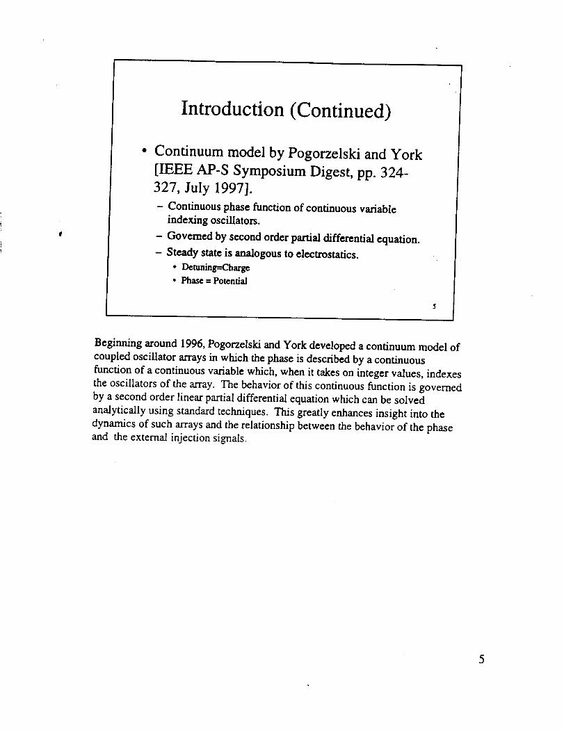
Continuum model by Pogorzelski and York

[IEEE AP-S Symposium Digest, pp. 324-327, July 1997].

- Continuous phase function of continuous variable

indexing oscillators.

- Governed by second order partial differential equation.

- Steady state is analogous to electrostatics.

• Detuning=Charge

• Phase = Potential

Beginning around 1996, Pogorzelski and York developed a continuum model of

coupled oscillator arrays in which the phase is described by a continuous

function of a continuous variable which, when it takes on integer values, indexes

the oscillators of the array. The behavior of this continuous function is governed

by a second order linear partial differential equation which can be solved

analytically using standard techniques. This greatly enhances insight into the

dynamics of such arrays and the relationship between the behavior of the phaseand the external injection sig-nals.

The M by N Array

-M-1 -M -M+I -M+2 p M M+I

_x

This diagram schematically represents a (2M+l) by (2N+l) array of oscillators

coupled to nearest neighbors. This is the array to be analyzed in the following.The oscillators shown in dashed lines are external sources which provide the

properly phased injection signals to the perimeter oscillators of the array.

6

The Continuum Model

Begin with Adler's theory applied to the

array.

a6,j ,, -"_t =c°,,,_,.,_ - E EAc°_,_.,,,,sin(O,j.,,,,, +go-O,,,,,)

m,s-M n1-N

M N

-2 +oo-e,,)p,i-M qm-N

Define the phase by:

_ij -" O')rcf f "b _i)

To derive the continuum model of this two dimensional array, we begin with

Adler's description of the injection locking phenomenon. In his theory, the time

derivative of the phase of an injection locked oscillator is related to the sine of

the phase difference between the oscillator signal and the injection signal.

Generalizing this to the two dimensional array of mutually injection locked

oscillators (with general interoscillator coupling topology) we arrive at the

system of differential equations shown. We then define the phase, phi, as shown

relative to a reference frequency which can be chosen arbitrarily.

The second double summation represents the externally provided injectionsignals.

7

or,

The Continuum Model (Cont.)Then,

dt - a).,,_j - co,, I - _E sin((1)j ,. + _j - ¢1,,. )_-I n=J-I

M #

p'-M q--N

- a),_4 - a),¢ + ga)_,, [¢i_,j_, + __,.,., +_+,j_, + _+,.j+, -4_]

M N

q=-M p=-N

Using this def'mifion of phi the system of equations become that shown here.

Then, assuming that the locking ranges are all the same, that the coupling phase

is zero, and that the phase differences between adjacent oscillators is small, we

can linearize the system as shown. Then, the quantity in the square brackets can

be identified as the finite difference approximation to the Laplacian operator.

8

The Continuum Model (Cont.)

which leads to,

,_¢) ,9'¢ 0¢"_-'7 + "_"i- - V ( x, y ) _ - -_ _

0.}#,,_ -- COref

A oJ tockV(x,y)¢_j(x,y;r)

where,

Z = AgOto_ t

Thus, defining a continuous phi function and continuous variables x and y

indexing the oscillators, we arrive at the partial differential equation for phi

shown. V represents the distribution and strength of the injection signals with

phase phi_,j. Tau is time measured in inverse locking ranges.

9

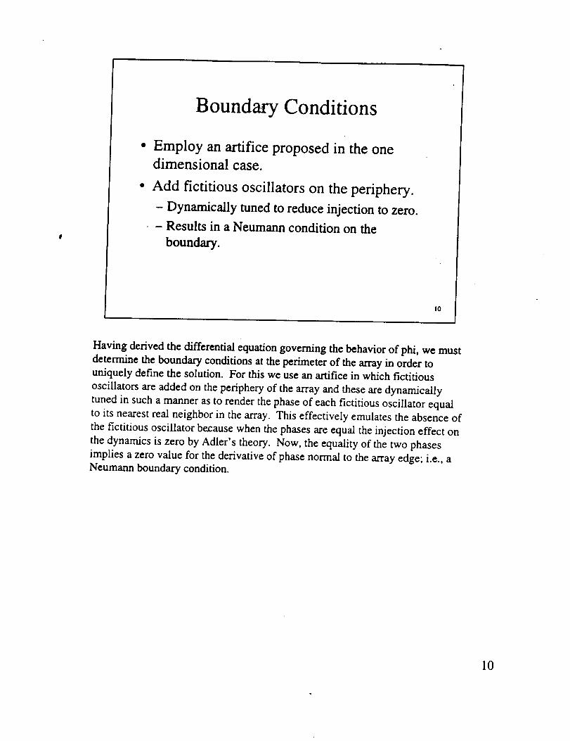
Boundary Conditions

Employ an artifice proposed in the one

dimensional case.

Add fictitious oscillators on the periphery.

- Dynamically tuned to reduce injection to zero.

- Results in a Neumann condition on the

boundary.

10

Having derived the differential equation governing the behavior of phi, we must

determine the boundary conditions at the perimeter of the array in order to

uniquely define the solution. For this we use an artifice in which fictitious

oscillators are added on the periphery of the array and these are dynamically

tuned in such a manner as to render the phase of each fictitious oscillator equal

to its nearest real neighbor in the array. This effectively emulates the absence of

the fictitious oscillator because when the phases are equal the injection effect on

the dynamics is zero by Adler's theory. Now, the equality of the two phases

implies a zero value for the derivative of phase normal to the array edge; i.e., aNeumann boundary condition.

10

The M by N Array

-M-I -M -M+I -M+2 p M M+I

IL XI1

i

This diagram illustrates the fictitious oscillator arrangement used in theboundary condition derivation.

I1

Injection of Perimeter Oscillators

V(x, y) = C P(x) + C Q(y)

C P(x)= n,,,_(x-x:)+n._,5(x- x_)

• +CQ(y)=ny,8(y- y,) n:, 8(y- y_)

12

We intend to supply externally derived injection signals only to the oscillators

on the perimeter of the array. This implies that the function F takes the form

shown. C measures the strength of the injection signals and is measured in

terms of the implied locking rangerelative to the inter-oscillator locking range.

12

The Differential Equation

'92_ '_¢ ,9¢oax--"Y+ --_--F-CP(x)O- CQ(y)O-

= -CP(x)_ (x,y;"c)- CQ(y)O_j(x, y;"t')

13

For the case of perimeter injection, the differential equation governing the phase

dynamics takes the form shown. This equation will be solved by means of a

Green's function, G; that is, a solution for the case of a delta function source

term. The Green's function will be expressed as a sum of the eigenfunctions ofthe operator in the classical manner.

13

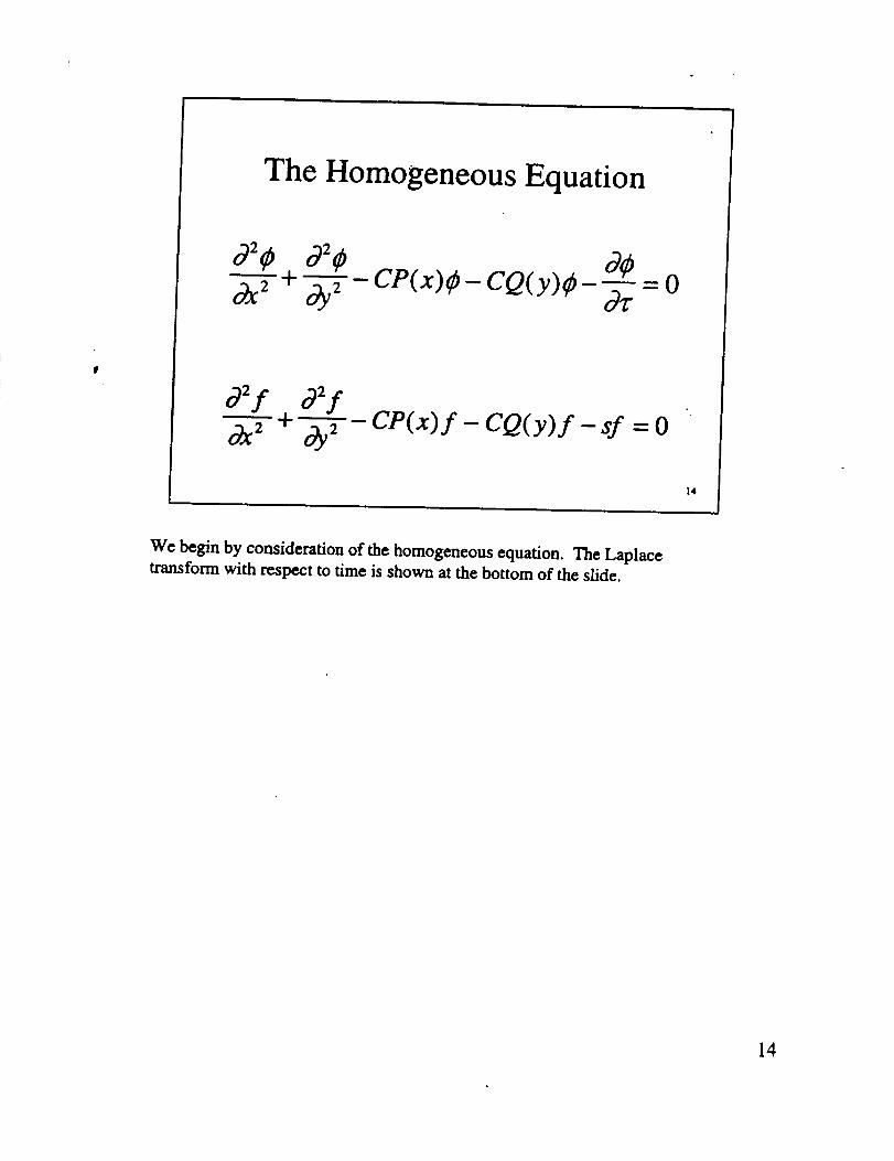
The Homogeneous Equation

'9_0 9_0 ,90-_ + oaY2 - CP(x)O- CQ(Y)O- Oz"-0

092f 032f

--_ +-"_-- CP(x) f - CQ(y) f - sf = 0

14

We begin by consideration of the homogeneous equation. The Laplacetransform with respect to time is shown at the bottom of the slide.

14

Separation of Variables

Let f(x,y) = X(x, sx)Y(y,sy).

Then, X " - CPX - s xX = 0

Y"- CQY- syY = 0

where, s = sx + sy.

X"- t2x,_(x- x:) - f_ _(x- xD- sxX = 0

Y"-_,,8(y- y:)- _, 8(y- y_)- s,Y = o

15

The homogeneous equation can be solved by the classical separation of variables

method. We assume a product solution and obtain two ordinary second order

differential equations for the x and y dependences of the solution. Substitutingthe deisred form of the V function results in the equations shown at the bottomof the slide.

15

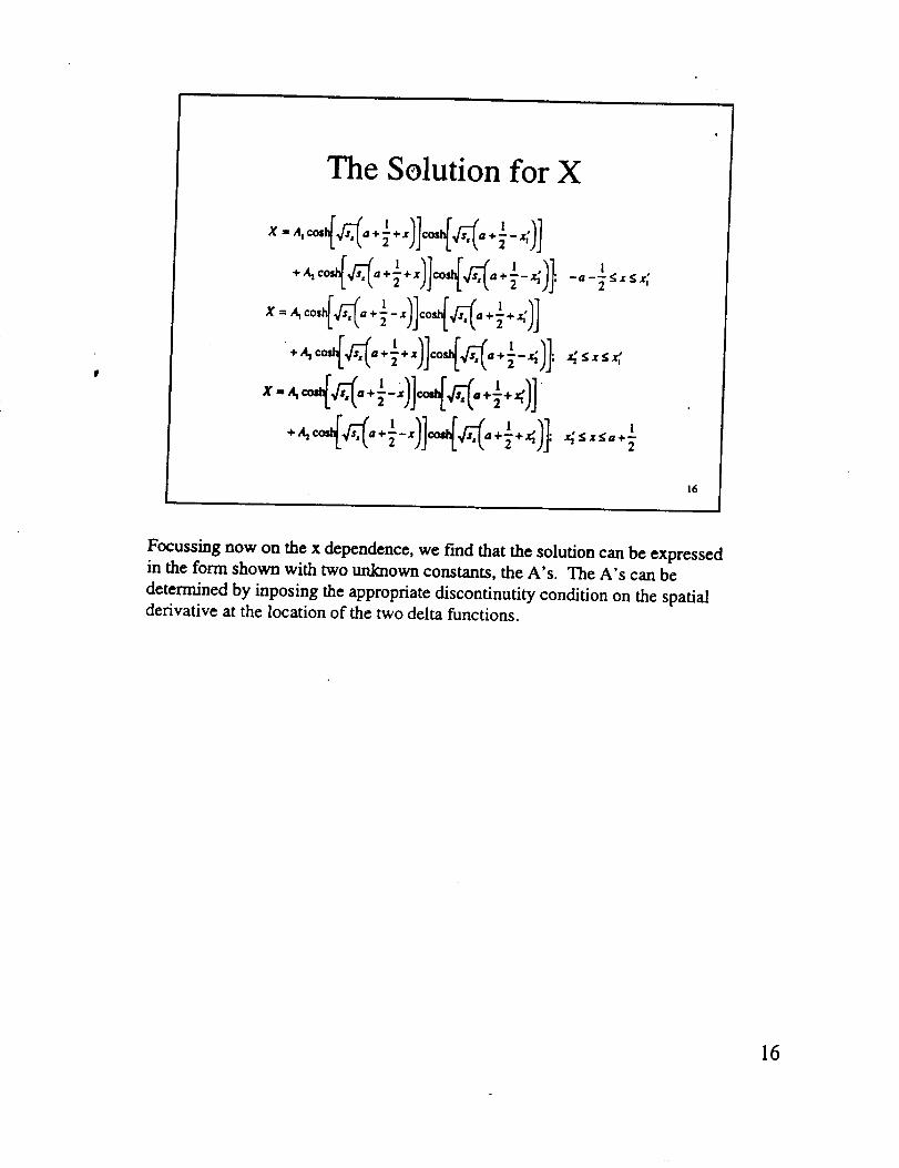
The Solution for X

1 1 ,+ A2cos_a+-_+xllco_a+-_-x111;

l l ,

• l l ,_ Sx_x_

16

Focussing now on the x dependence, we find that the solution can be expressedin the form shown with two unknown constants, the A's. The A's can be

determined by inposing the appropriate discontinutity condition on the spatialderivative at the location of the two delta functions.

16

Evaluation of the A's

At the delta's,

which yields,

x .x_-= _, X(x;)

[MM_I M,,I[A, 1

17

The discontinuity conditions are shown here. These, when applied to the

solution, provide a homogeneous set of simultaneous linear equations for the

A's. For a solution to exist, the determinant of the coefficients matrix must bezero.

17

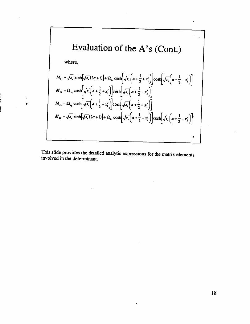
Evaluation of the A's (Cont.)

where,

I , I

Mr,--Vl'_sinh[_'_(2a+l)]+t2. cosh[ _'_ Ia + -_ + x, l J cosh[ _a + _ _ x [) J

1 ,M,. =.., cosh_a+_+xt3]cosh[_a+l_x_) ]

1 , +1 , .

18

This slide provides the detailed analytic expressions for the matrix elementsinvolved in the determinant.

18

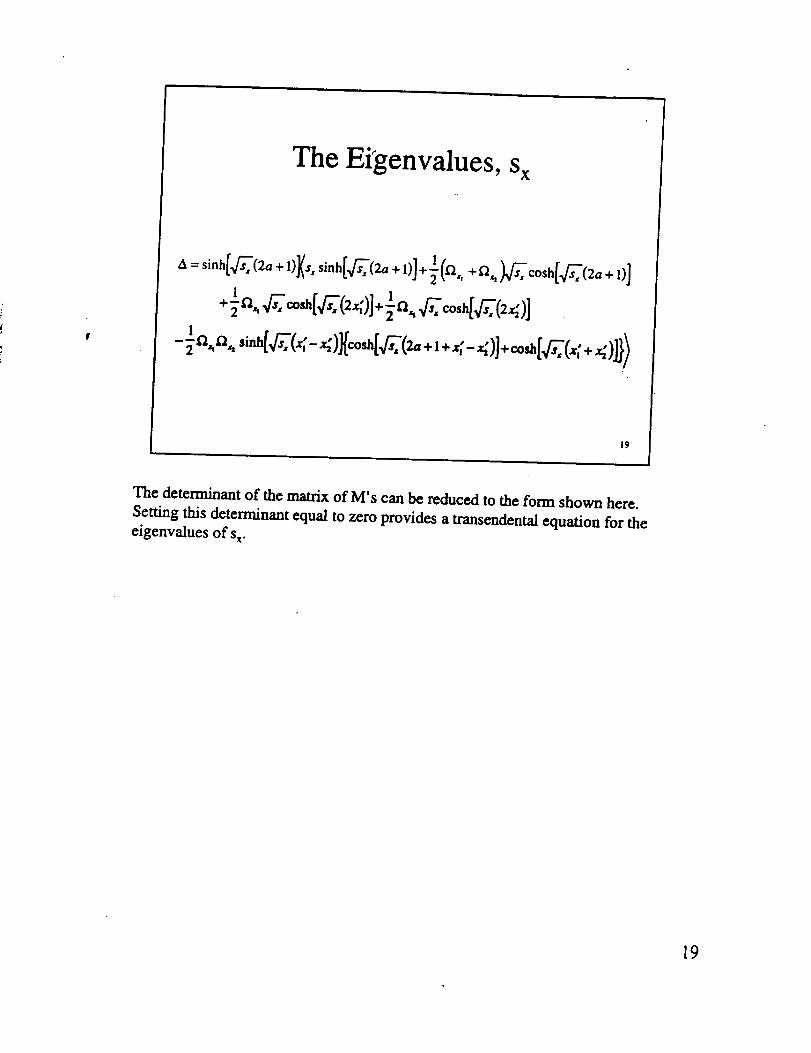
The Eigenvalues, sx

19

The determinant of the matrix of M's can be reduced to the form shown here.

Setting this determinant equal to zero provides a transendental equation for theeigenvalues of s x.

19

Eigenfunctions

or

yields

• 1

2O

Once the eigenvalues are found, the homogeneous equations represent two

relationships between the A's, each of which give a solution. These two

solutions differ only by a multiplicative constant. However, this constant can, in

certain cases, be zero for one of the solutions, indicating that the appropriate

normalization constant is infinite. In such cases it is expedient to use the othersolution.

The solution shown is, iri fact, a linear combination of the two solution chosen to

create a symmetric looking expression. For normalization reasons as described

above, two options are represented; I.e., eta equal to one or minus one. The

normalization integrals of the square of this function over the extent of the array

can be carried out analytically because they only involve products of hyperbolicfunctions of x. The actual expressions are, however, a bit cumbersome.

20

Eigenfunctions (Cont.)

• Similar procedure yields the y dependenteigenfunctions.

• The Green's function can now be written in

terms of these two sets of functions.

• The Green's function has no direct physicalsignificance in this instance.

• It will be used to obtain the physicallymeaningful solution.

21

Carrying out the same solution procedure for y yields the set of y dependent

eigenfuncdons. Multiplying the x and y dependent functions gives a doubly

infinite set of normalized two dimensional eigenfunctions in terms of which theGreen's function may be expressed.

It is noted that this Green's function is the solution of the differential equation

with a delta function source. However, because the equation we are solving has

line sources instead of point sources, it is necessary to integrate the Green's

function over the sources to obtain a physically meaningful expression for thephase.

21

The Green's Function

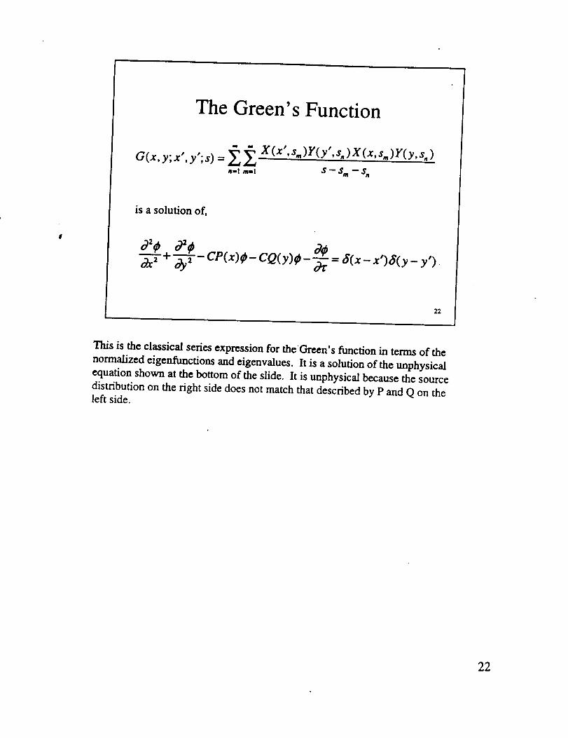
G(x, y;x', y';s) = _ _ X(x',s.)Y(y',s.)X(x,s.)Y(y,s_)

•-J ..l s-s, -s_

is a solution of,

0324 a92_ CQ(y)_-_"_" +-_-r- CP(x)_- = ,_(x- x'),_(y - y')

22

This is the classical series expression for theGreen's function in terms of the

normalized eigenfunctions and eigenvalues. It is a solution of the unphysical

equation shown at the bottom of the slide. It is unphysical because the source

distribution on the right side does not match that described by P and Q on theleft side.

22

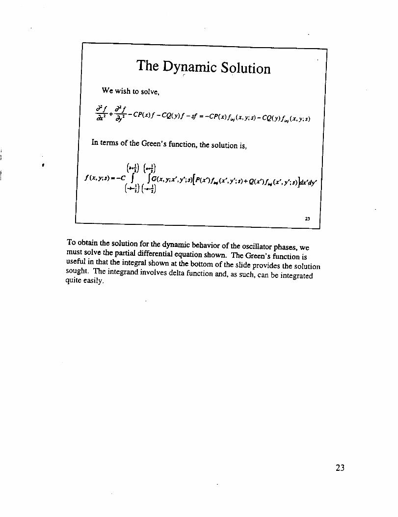
The DYnamic Solution

We wish to solve,

_f _I-_- + _- CP(x)I - CQ(y)f - sf = -CP(x)f_, i (x, y; s) - CQ(y)fai (x, y; s)

In terms of the Green's function, the solution is,

i_,.,,;,_=_c('_)(.4)(-'4][_,.,;,,'. y';,)[pcx')J',.,c.,',y'.,>+o_,'),-,.,_.,,.y,.,)_,e,

23

To obtain the solution for the dynamic behavior of the oscillator phases, we

must solve the partial differential equation shown. The Green's function is

useful in that the integral shown at the bottom of the slide provides the solution

sought. The integrand involves delta function and, as such, can be integratedquite easily.

23

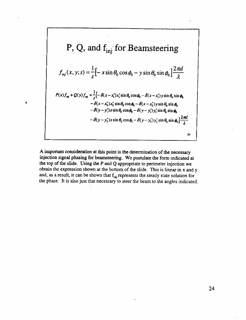
P, Q, and finjfor Beamsteering

2ridl[-xsinOoc°SOo- ysinOosinOo]f_s(x, y;s) = s

l --

P(x)L¢ + Q(y)f,_ = _[- 8(x- x;)x_ sinOocos¢o -8(x- x_)y sin0o sin¢o

- 6(x- x_)x_ sine o cosCb -8(x-x_)ysi.8 o sinCb

- 8(y - y_)x sin 0o cos #o - 8(y - y_)y_ sin 0o sin ¢h

.... ,2az/- Z/(y - y_)x sin 8o cos ¢h - 8(y - Y2)Y, sin 80 sm ¢b]'_

24

A important consideration at this point is the determination of the necessaryinjection signal phasing for beamsteedng. We postulate the form indicated at

the top of the slide. Using the P and Q appropriate to perimeter injection we

obtain the expression shown at the bottom of the slide. This is linear in x and y

and, as a result, it can be shown that fi,j represents the steady state solution for

the phase. It is also just that necessary to steer the beam to the angles indicated.

24

The Dynamic BeamsteeringPhase Solution

_)(x,y;_)=_R,,,,,(x,y)[1-e("÷_')r}_(_)nml m*,l

which converges slowly. The convergence rate

can be improved by adding and subtracting the

known steady state solution. That is,

25

Substituting the beamsteering source function into the integral expression for the

solution and carrying out the integrations, which can be done analytically, we

obtain the series expansion for the solution. Each term of the series has a pole in

the complex plane the location of which is given by the eigenvalue

corresponding to that term. The inverse Laplace transform can thus be obtained

by residue calculus and the solution in the time domain expressed as the residueseries shown.

25

The Dynamic Beamsteering

Phase Solution (Cont.)

lira r

and the solution may be written in the form,

_(x,y;_')= _,..--._R,=(x,y)[-e("÷')_]u(r)- (xsin0ocos_ + ysineosin_ )-_

26

The rate of convergence of the residue series can be increased by subtracting the

steady state value of the series terms and then adding the known steady statesolution to the result. This procedure is illustrated in this slide.

26

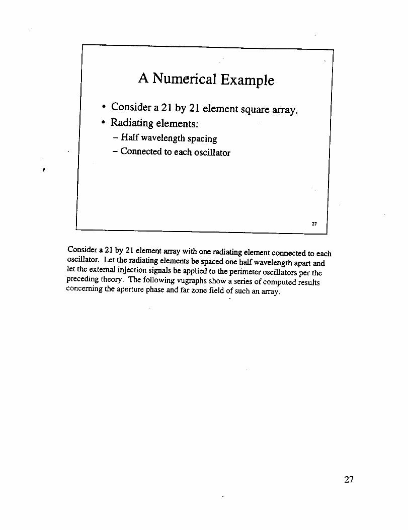
A Numerical Example

° Consider a 21 by 21 element square array.

° Radiating elements:

- Half wavelength spacing

- Connected to each oscillator

27

Consider a 21 by 21 element array with one radiating element connected to each

oscillator. Let the radiating elements be spaced one half wavelength apart and

let the external injection signals be applied to the perimeter oscillators per the

preceding theory. The following vugraphs show a series of computed results

concerning the aperture phase and far zone field of such an array.

27

galII m mln m _l_l,

2$

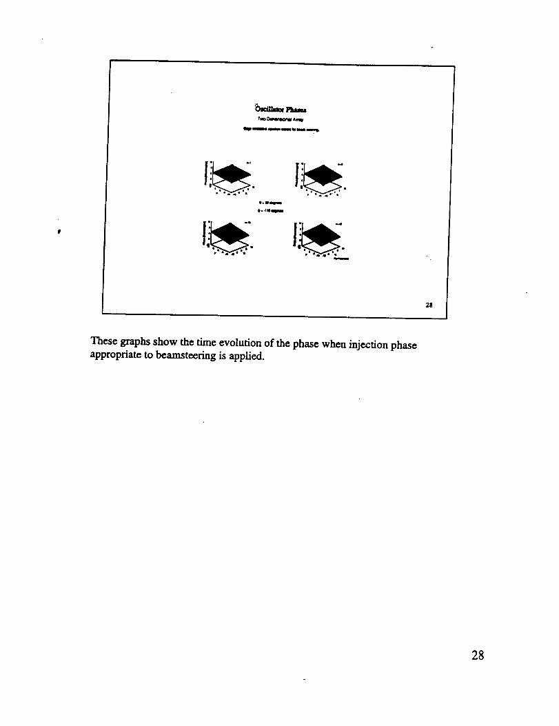
These graphs show the time evolution of the phase when injection phaseappropriate to beamsteering is applied.

28

3O

2O

I0

0

) -I0

-2O

,'

E)

.so-_o-_o o _o _ soAng_,n Degrees

29

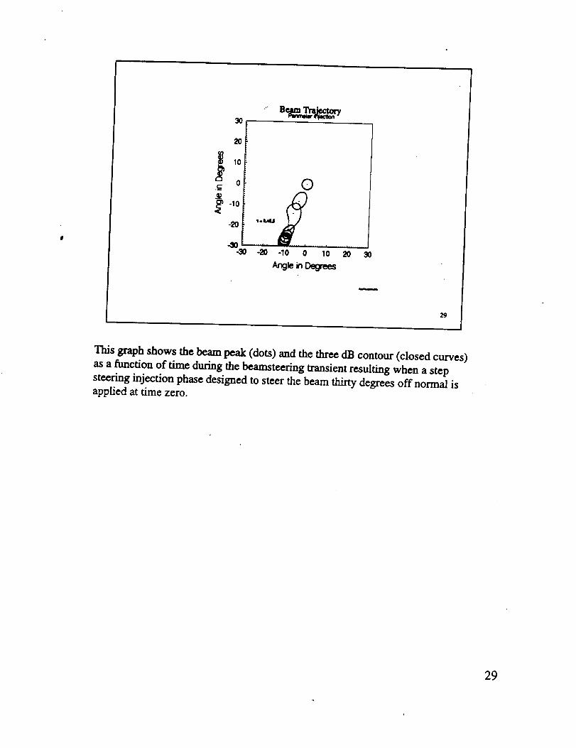
Thisgraphshows thebeam peak (dots)and thethreedB contour(closedcurves)

asa functionoft/me duringthebeamstecr/ngtransientresultingwhen a stepsteeringinjectionphasedesignedtostccrthebeam thirtydcgrcesoffnormal isappliedattimezero.

29

-_- 26 " '" ' '_'_"

_ :...._,,."

18 _ s_} 41,-.-ed.B_

16 -,m.,.,,a,,a._e..'_0 10 20 3O 4O 5O

T,_e [lr_rse Lcx:_gFUr_jes]

3O

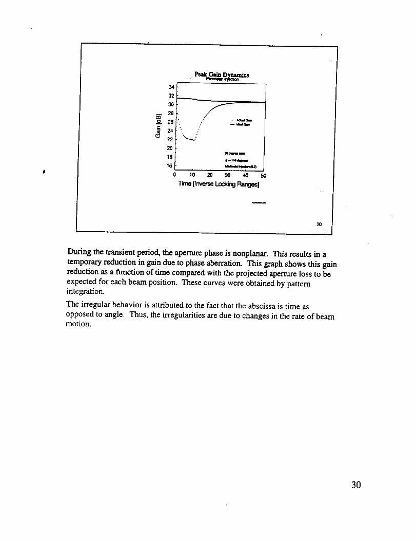
During thetransientperiod,theaperturephaseisnonplanar.Thisresultsina

temporaryreductioningainduc tophaseaberration.Thisgraphshows thisgain

reductionasa functionoftimecompared withtheprojectedaperturelosstobc

cxpectcdforeach beam position.These curvcswcrc obtaincdby pattcrnintegration.

Thc irregularbchaviorisattributcdtothefactthattheabscissaistimc as

opposed toangle.Thus,thcirrcgulariticsarcduc tochangcsintheratcofbeammotion.

3O

e-

31

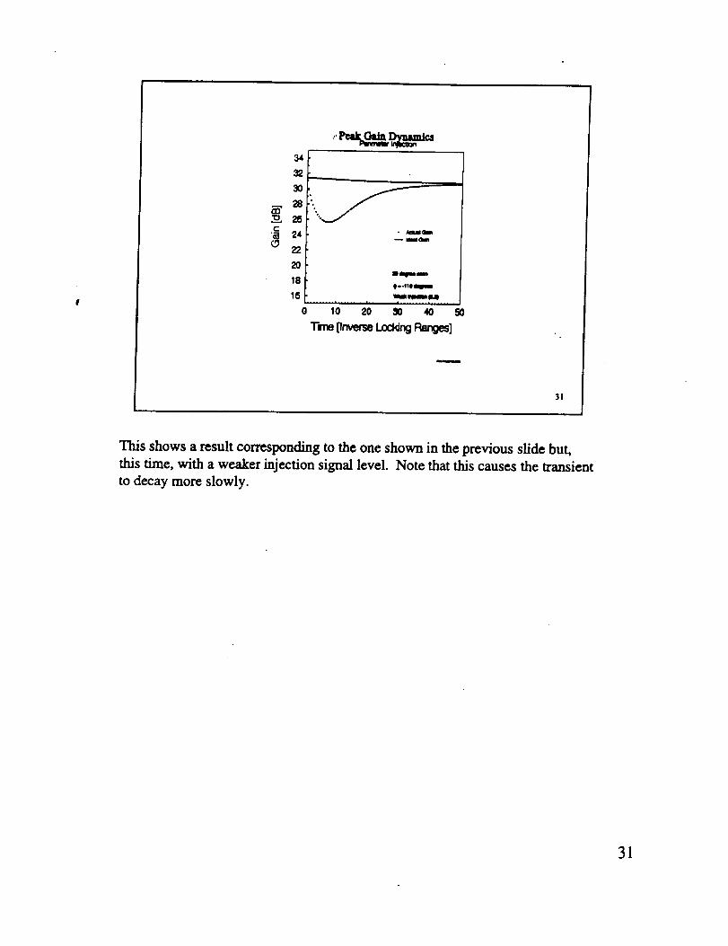
This shows a result corresponding to the one shown in the previous slide but,this time, with a weaker injection signal level. Note that this causes the transient

to decay more slowly.

31

34

30

e-

22

2O

18

18

_ =lmlOlm

_lal=mmm

10 20 30 40 GO

"_e [lnverseL.oe_ P,er_es]

32

This shows a result corresponding to the one shown in the previous slide but,this time, with a stronger injection signal level. Note that, while this causes the

transient to decay more rapidly, the gain dip is deeper and the peak moves moreerratically in this case.

32

30

2O

Beam TrajectoryPenme[er I_ject_

-30-30 -20 -10 0 10 20 30

Angle in Degrees33

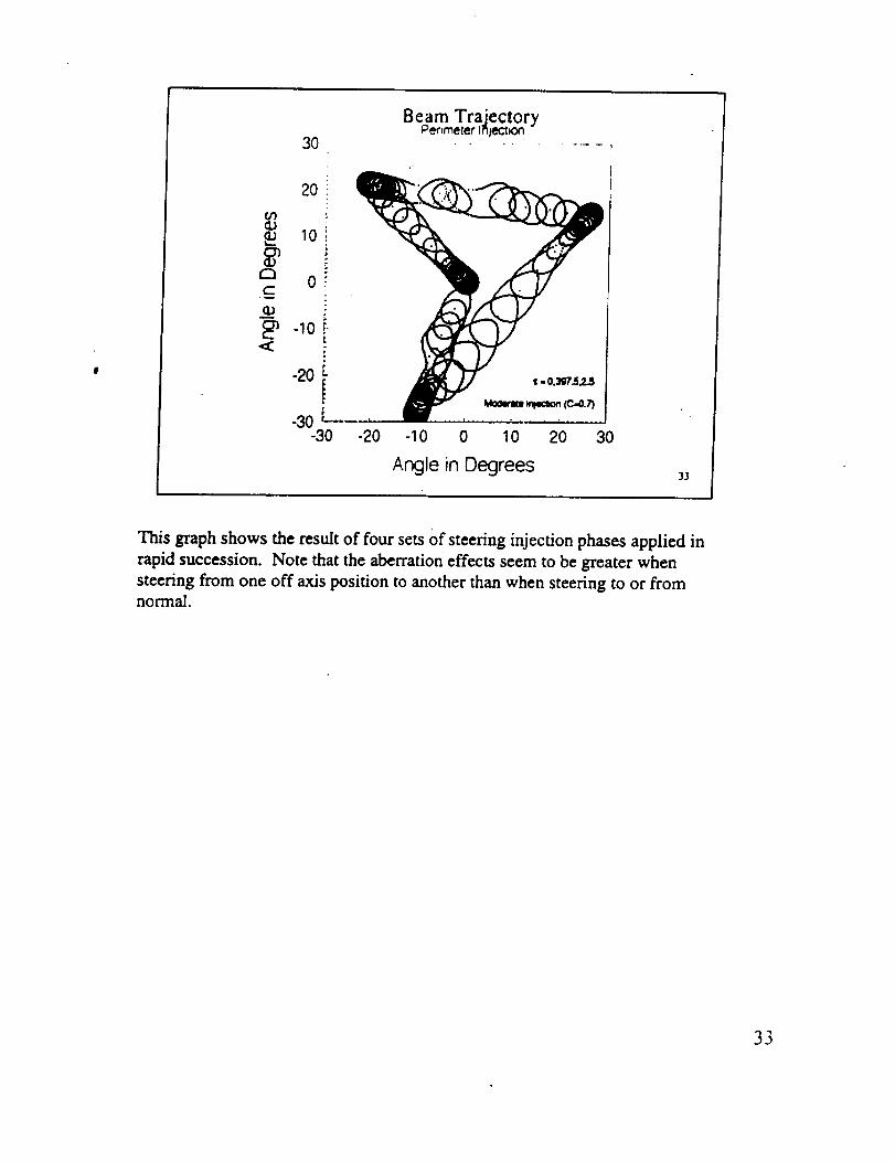
This graph shows the result of four sets of steering injection phases applied in

rapid succession. Note that the aberration effects seem to be greater when

steering from one off axis position to another than when steering to or fromnormal.

33

Concluding Remarks

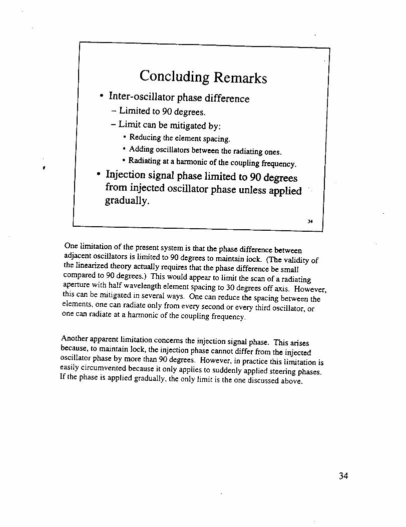
° Inter-oscillator phase difference

- Limited to 90 degrees.

- Limit can be mitigated by:

• Reducing the element spacing.

• Adding oscillators between the radiating ones.

• Radiating at a harmonic of the coupling frequency.

• Injection signal phase limited to 90 degrees

from injected oscillator phase unless appliedgradually.

34

One limitation of the present system is that the phase difference between

adjacent oscillators is limited to 90 degrees to maintain lock. (The validity ofthe linearized theory actually requires that the phase difference be small

compared to 90 degrees.) This would appear to limit the scan of a radiating

aperture with half wavelength element spacing to 30 degrees off axis. However,

this can be mitigated in several ways. One can reduce the spacing between the

elements, one can radiate only from every second or every third oscillator, or

one can radiate at a harmonic of the coupling frequency.

Another apparent limitation concerns the injection signal phase. This arises

because, to maintain lock, the injection phase cannot differ from the injected

oscillator phase by more than 90 degrees. However, in practice this limitation is

easily circumvented because it only applies to suddenly applied steering phases.

If the phase is applied gradually, the only limit is the one discussed above.

34