Two Classes Signals Signals are subdivided into two classes, namely, □ Deterministic signals □ Random signals Deterministic Signals & Random Signals Signals that can be modeled exactly by a mathematical formula are known as deterministic signals. Deterministic signals are not always adequate to model real-world situations. Random signals, on the other hand, cannot be described by a mathematical equation; they are modeled in probabilistic terms. In this chapter we shall use the power of MATLAB to describe some fundamental aspects of random signals.

Pseudo-random Numbers - Commands: “rand” & “randn” It’s fairly easy to generate uncorrelated pseudo-random sequences. MATLAB has two built-in functions to generate pseudo-random numbers, namely rand and randn. The rand function generates pseudo-random numbers whose elements are uniformly distributed in the interval (0,1). You can view this as tossing a dart at a line segment from 0 to 1, with the dart being equally likely to hit any point in the interval [0,1]. The randn function generates pseudo-random numbers whose elements are normally distributed with mean 0 and variance 1 (standard normal). Both functions have the same syntax. For example, rand(n) returns a n-by-n matrix of random numbers, rand(n,m) returns a n-by-m matrix with randomly generated entries distributed uniformly between 0 and 1., and rand(1) returns a single random number.

Practice

- Random Number Generation: Pseudo-random Numbers - >> %Generate one thousand uniform pseudo-random numbers >>rand(1,1000) % return a row vector of 1000 entries>>%Generate one thousand gaussian pseudo-random numbers >>randn(1,1000); % return a row vector of 1000 entries

272

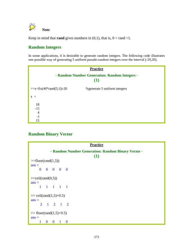
��Note�� Keep in mind that rand gives numbers in (0,1), that is, 0 < rand <1. Random Integers In some applications, it is desirable to generate random integers. The following code illustrates one possible way of generating 5 uniform pseudo-random integers over the interval (-20,20).

Practice

- Random Number Generation: Random Integers - (1)

>>x=fix(40*rand(5,1))-20 %generate 5 uniform integers

x =

18 -11 4 -1 15 Random Binary Vector

Practice

- Random Number Generation: Random Binary Vector - (1)

>>floor(rand(1,5)) ans = 0 0 0 0 0 >>ceil(rand(0,5)) ans = 1 1 1 1 1 >> ceil(rand(1,5)+0.5) ans =

2 1 2 1 2

>> floor(rand(1,5)+0.5) ans =

1 0 0 1 0

273

Practice

- Random Number Generation: Random Binary Vector - (2)

Write a MATLAB script to generate M sequences of N coin flips each.

>>M=10; >>N=20; >>C=floor(rand(N,M)+0.5) >>% count the # of heads (1s) in each >>% column (sequence of N trials)?

It is a good practice to provide a seed before using the rand command; otherwise you will get the same sequence of random numbers every time you restart the computer. A good way to reseed the random number generator is to use the clock, as follows: >>rand(‘state’, sum(100*clock)); If every time you start MATLAB, you type the command above, your random numbers will be truly random, otherwise they will be pseudo-random.

The “hist” Command When the probability density function (pdf) is not available, it can be estimated using a histogram. A histogram is constructed by subdividing the interval [a,b] containing a collection of data points into sub-intervals known as bins and count for each bin the number of the data points that fall within that bin. The function hist provides the histogram of sample values of a random variable. � Syntax >>[n,y]=hist(x,N); The function hist divides the interval [min(x), max(x)] into N bins and yields the output [n,y], where n is a vector whose elements are the number of samples in each bin, and y is a vector whose elements are the centers of the bins. When used in this manner, the hist function does not produce a graph; instead we use the bar function. The bar function produces a bar graph which for each value of y, there is a bar whose height is proportional to n.

274

The “bar” Command Bar graphs are a good way of examining trends (rising or falling) in one or more variables over a period of time. MATLAB bar graphs can be created to plot either vertically or horizontally. The bar function produces a bar graph which for each value of y, there is a bar whose height is proportional to n.

Practice

- Bar Graphs- (1)

Generate 10000 gaussian distributed pseudo-random numbers, and then plot the histogram.

>>%Generate 10000 gaussian pseudo-random numbers and draws a histogram >>x=randn(1,10000); % generate a random vector >>N=30; % specify the number of bins >>[n,y]=hist(x,N); % y=vector of centers of bins; n=centers of bins>>bar(y,n) % plot histogram using the bar function >>xlabel(‘Realization of random variable’) >>ylabel(‘Number of occurrences’)

275

Practice

- Bar Graphs- (2)

Find the approximate distribution of two resistors in a parallel connection assuming that they each have measured values, which vary uniformly about their nominal values by . 5%±

1

2

1 21 2

1 2

105

//eq

R kR k

R RR R RR R

= Ω= Ω

= =+

Compute 10000 trials and histogram the results.

n=10000; r1=rand(n,1)*(10500-9500)+9500; r2=rand(n,1)*(5250-4750)+4750; r3=r1.*r2./(r1+r2); subplot(2,1,1);hist(r3,20) title('Histogram of random resistor values in parallel','FontSize',14); ylabel('Occurence R1//R2', 'FontSize',14) xlabel('Range of R3 values','FontSize',14)

Scatter Digram The scatter diagram is a useful tool for identifying a potential relationship or correlation between two variables. Correlation implies that as one variable changes, the other also changes. Sometimes if we know that there is good correlation between two variables, we can use one to predict the other.

276

Practice - Scatter Diagram-

(1) >>x=rand(100,1); >>y=x+rand(100,1); >>plot(x,y,’o’,’MarkerSize’,2) %2-D scatter plot >>corrcoef(x,y); >>z=randn(100,1); >>plot3(x,y,z,’.’); %3-D scatter plot

Practice

- Scatter Diagram- (2)

>>x=raud(20,1); >>y=rand(20,1); >>scatter(x,y)

Practice - Scatter Diagram-

(3) >>%scatter plot of 2-D gaussian variates

>>%with unit covariance >>x=randn(1000,2); >>scatter(x(:,1),x(:,2),’.’) >>set(gca,’FontSize’,15)

277

Correlation Coefficient The correlation coefficient is a measure of the degree of linear relationship that exists between two variables. When using the corrcoef function, MATLAB produces four correlation values. These are xyr , xxr , yyr and yxr . We are only interested in the correlation between x and y, so instead of writing just r, we write r(1,2) to indicate that we are interested in the number positioned in the first row, second column of the matrix r.

Practice

- Correlation Coefficient (1)

% compute the correlation coefficient of x and y x=[1 2 3 4 7]; y=[3 5 6 9 8]; r=corrcoef(x,y); disp([‘The correlation coefficient between x and y is: ‘, num2str(r(1,2))])

Practice

- Correlation Coefficient (2)

>>x=[0:10]; >>y=5*x+4; >>r=corrcoef(x,y)

r = 1.0000 1.0000 1.0000 1.0000

Practice

- Correlation Coefficient (3)

>>x=[0:10]; >>y=-5*x+4 >>r=corrcoef(x,y); >>r(1,2) ans = -1.0000

278

Introduction -Commands: “mean”, “std” & “median” Many times we wish to characterize the probability density function (pdf) with a few numbers. The mean is a measure of the center or most likely value of a distribution. The variance and standard deviation are a measure of the extent to which a distribution varies from its mean, and the median is also a measure of the center. These quantities describe a trend and the variation of the data about that trend. The median is less sensitive to extreme scores (outliers) than the mean. The MATLAB commands mean, std, and median determine the sample mean, standard deviation, and median, respectively. The standard deviation is measured in the same units as the mean and the median.

Practice

- Mean, Standard Deviation & Median-

>>x=randn(1,10000); % generate gaussian numbers >>[mean(x); std(x); median(x)] % compute the mean, standard deviation, and median

ans =

0.0066 1.0036 0.0098

Normal Distribution It is a straightforward matter to simulate from any normal distribution with a specified mean value and a specified standard deviation. In MATLAB one can produce normally distributed numbers with mean zero and a standard deviation of unity directly using the function randn. To produce random numbers from a gaussian distribution of mean m and a standard deviation of sd, proceed as follows: >>r=randn; % gaussian number: mean zero, standard deviation unity >>z=m+r*sd; % gaussian number: mean m, standard deviation sd. The rand function generates random numbers uniformly distributed from zero to one. Numbers uniform on the interval [0,1] can be transformed to numbers uniform on [a,b] using the following transformation: >>r=rand; % uniform number in [0,1] >>x=(b-a)*r+a; % uniform number in [a,b]

279

For a gaussian random variable X with mean m and standard deviation s, the cumulative distribution function is given by

( ) { } 1 12 2 2X

x mF x P X x erfs−⎛ ⎞= ≤ = + ⎜ ⎟

⎝ ⎠

where erf is the error function. MATLAB has a built-in error function erf defined by

( ) 2

0

2 x terf x e dtπ

−= ∫

The following results are important when evaluating gaussian probabilities:

{ } 2 11 2

1 12 22 2

x m xP x X x erf erfs s− −⎛ ⎞ ⎛< ≤ = −⎜ ⎟ ⎜

⎝ ⎠ ⎝

m ⎞⎟⎠

{ } { } 1 112 2 2

x mP X x P X x erfs−⎛ ⎞> = − ≤ = − ⎜ ⎟

⎝ ⎠

Practice

- Gaussian Probabilities- A gaussian voltage has a mean value of 5 and a standard deviation of 4. 1. Find the probability that an observed value of the voltage is greater than zero. 2. Find the probability that an observed value of the voltage is greater than zero but less than or

equal to 5. >>% Answer to part (1) >>m=5; s=4; x=0; % specify the mean, standard deviation, and x>>z=(x-m)/(s*sqrt(2)); % define an intermediate variable z >>P1=1/2-1/2*erf(z) % compute P(X>0) >>%Answer to part (2) >>x1=0; x2=5; % define the values of x1 and x2 >>z1=(x1-m)/(s*sqrt(2)); z2=(x2-m)/(s*sqrt(2)); % define two intermediate variables P2=1/2*erf(z2)-1/2*erf(z1); % compute the probability { }0 5P X< ≤

280

Uniform White Noise A uniform white noise is a sequence of independent samples with zero mean. The rand function generates a sequence of uniform pseudo numbers with mean of 0.5 and variance of 1/12. Therefore, the average power of (rand-0.5) is 1/12. A uniform white noise with a specific average power P can be generated using ( )12 rand 0.5P − . Gaussian White Noise Similarly, the function randn provides a gaussian sequence with zero mean and a variance of unity. Therefore, one can generate a white gaussian noise having an average power P via

randnP .

Practice

- White Noise- (1)

>>%Signal-to-noise ratio=2 >>t=[0:512]/512; %define a time vector >>signal=sqrt(2)*cos(2*pi*5*t); %define a signal sequence (average power=1 W) >>noise=sqrt(0.5)*randn(1,length(t)); %define a noise sequence (average power=0.5 W) >>sn=signal+noise; %compute the signal+noise sequence >>subplot(2,1,1);plot(t,sn);grid %plot the signal+noise sequence >>%Signal-to-noise ratio=20 >>signal2=sqrt(20)*cos(2*pi*5*t); %define a signal sequence (average power=10 W) >>sn2=signal2+noise; %computer the signal+noise sequence >>subplot((2,1,2);plot(t,sn2);grid %plot the signal+noise sequence >>legend(‘snr=20’,’snr=2’); %add legend to plot

281

Practice

- White Noise- (2)

Consider a signal consisting of two sinusoids having frequencies 220 Hz and 220*2 1/12 Hz and amplitudes 1.5V and 20V, respectively. This signal is corrupted by an additive white noise. Complete the signal to noise ratio.

>>t=(0:4095)/1000; >>s1=1.5*sin(2*pi*220*t); >>s2=20*sin(2*pi*220*2.^(1/12)*t); >>b=randn(1,length(t)) >>s=s1+s2+b >>figure(1); plot(t,s); title(‘signal’); pause; >>figure(2); psd(((s-mean(s)),256,1000, hamming(256)) >>sigmasin=sum(psd(((s1+s2)-mean(s1+s2),256))*2/256; >>sigmab=sum(psd((b-mean(b)),256)*2/256; >>rsb=10*log10(sigmasin/sigmab) >>%rsb=23dB

sort sum max min randint norm(x, arg)

reorders elements of a vector to ascending order computes the summation of a vector x finds the largest entry of the vector x finds the smallest entr of the vector x generates matrix of uniformly distributed random integers computes the norm of a matrix or a vector

��NOTE�� The commands max and min return the maximum and minimum values of an array, and with a slight change of syntax they will also return the indices of the array at which the maximum and minimum occur. >>[y,k]=max(y) % y=max; k=index >>[y,k]=min(y) % y=min; k=index

282

The “rand” Command The rand function is easy to use to simulate coin tosses by setting the probability of getting a head to be p, calling the function rand, and if rand gives a number less than p, a head is said to occur. A similar method applies to tossing a single die. In this case the cut-off values (for a fair die) would be 1/6, 2/6, 5/6. This procedure of simulating probabilistic events is often called Monte-Carlo Simulation.

Practice

- Spinning Coins: The “rand” Command-

N=input('Enter the number of tosses:') p=input('Probability of head on a single toss:') number_heads=0; number_tails=0; v=[ ]; for k=1:N

rand_number=rand; if rand_number<p fprintf('H') number_heads=number_heads+1; v=[v 1]; else fprintf('T') number_tails=number_tails+1; v=[v 0]; end end pro_head=number_heads/N; outcome=[number_heads number_tails]; disp('number & relative frequency of heads:') number_heads, prob_head,pause disp('number & relative frequency of tails:') number_tails, 1.-prob_head,pause number_bins=2; hist(v,number_bins) title('Histogram of Heads & Tails');

283

Tossing a Coin There are only two outcomes when tossing a coin, heads or tails. When a fair coin is spun, the likelihood of having heads or tails is 0.5. Since a value returned by the function rand is equally likely to be anywhere in the interval [0,1], we can represent heads, say, with a value less than 0.5, and tails otherwise. Following is a fragment of MATLAB code to display the outcomes in 30 simulated coin tosses.

Practice - Spinning Coins-

Simulate spinning a fair coin 30 times.

N=input(‘Enter the number of simulations: ‘) for k=1:N

rand_number=rand; if random_number<0.5 fprintf(‘ H ‘) else fprintf(‘ T ‘) end

end fprintf(‘\n’)

Rolling a Die There are 6 possible outcomes when rolling a die. Note that if rand generates a number 0<x<1 then x<6x<6, so if x is rounded up to the next integer, then a random integer from 1 to 6 is obtained. The MATLAB function ceil can be used to round x up, i.e., 1�ceil(6*x)�6.

Practice - Rolling Dice-

Write a script function that will simulate n throws of a pair of dice This entails the generation of random integers in the range 1 to 6. This can be accomplished as follows: floor(1+6*rand); function r=dice(n) %simulate n throws of a pair of dice %Input: n, the number of throws %Output: an n-by-2 matrix, each row corresponds to one throw %Usage: r=dice(3) r=floor(1+6*rand(n,2)); %end of dice

ans = 1 1

3 2 5 2

1 4 >>sum(dice(100))/100 % compute average value over 100 throws

284

Practice

- Monte Carlo approximation of π-

Consider the following diagram of quarter unit circle inside a unit square. The ratio of the area of the quarter circle to the area of the square is pi/4, so if we pick a point in the square at random, the probability of it landing within the circle is pi/4. This idea provides a simple way of approximating pi, by finding a sample proportion of random points falling in the circle and multiplying by 4.

Write a MATLAB script to estimate the value of pi.

function estimate=randpi(n) s=0; for k=1:n

if(rand^2+rand^2<=1) s=s+1; end

end estimate=4*(s/n);

Practice

-Information measure-

The average information measure of a digital source is defined by

( )21

log bitsn

k kk

H P P=

= −∑

where n is the number of possible distinct source messages and is the probability of sending the k-th message. This average information is often known as the source entropy.

kP

Example: A digital source puts out –1.0 V and 0.0 V levels with a probability of 0.2 each and 3.0 V and 4.0V levels with a probability of 0.3 each. Evaluate the entropy of the source.

>>p=[0.2 0.2 0.3 0.3]; % define the vector of probabilities >>H=-sum(p.*log2(p)) % compute the entropy

H =

1.9710

285

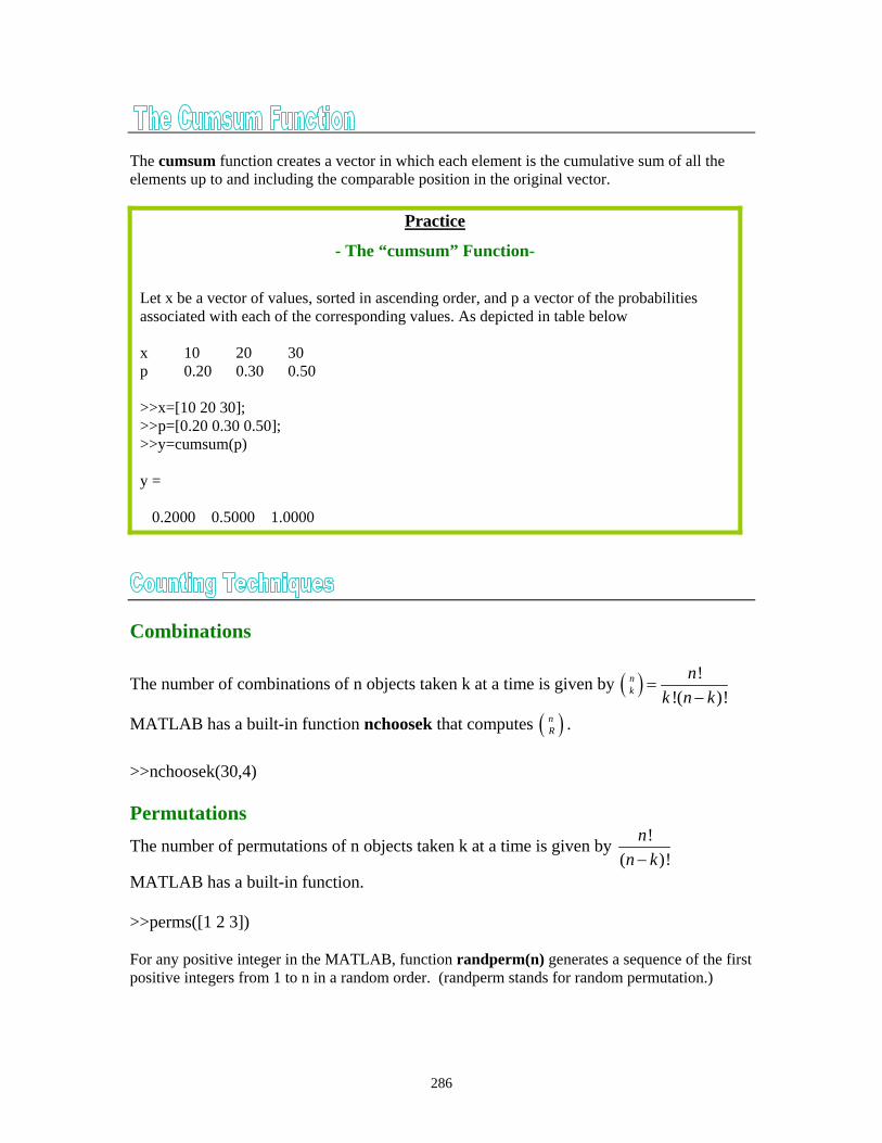
The cumsum function creates a vector in which each element is the cumulative sum of all the elements up to and including the comparable position in the original vector.

Practice

- The “cumsum” Function-

Let x be a vector of values, sorted in ascending order, and p a vector of the probabilities associated with each of the corresponding values. As depicted in table below

x 10 20 30 p 0.20 0.30 0.50

>>x=[10 20 30]; >>p=[0.20 0.30 0.50]; >>y=cumsum(p)

y =

0.2000 0.5000 1.0000

Combinations

The number of combinations of n objects taken k at a time is given by ( ) !!( )!

nk

nk n k

=−

MATLAB has a built-in function nchoosek that computes ( )nR .

>>nchoosek(30,4) Permutations The number of permutations of n objects taken k at a time is given by !

( )n

n k− !

MATLAB has a built-in function. >>perms([1 2 3]) For any positive integer in the MATLAB, function randperm(n) generates a sequence of the first positive integers from 1 to n in a random order. (randperm stands for random permutation.)

286

Practice

- Counting Technique: Permutations-

(1)

Use randperm function to simulate the rolling a die and outputting whether a 5 wasrolled or not.

die=randperm(6) if die(1)==5 disp('You rolled a 5') else

disp('You rolled something other than a 5') end

Practice

- Counting Technique: Permutations-

(2)

How do you generate permutation of numbers from 3 to 8? Ans: randperm(6)+2

( )!

! !nk

nCk n k

=−

If this expression is used, the factorials can get very big, causing an overflow. This can be avoided by using the following procedure: nck=1; n=input(‘Enter the value of n:’); k=input(‘Enter the value of k:’); for m=1:k nck=nck*(n-m+1)/m; end disp([‘nck=’, num2str(nck)’])

287

Practice

- Evaluation of Binomial Coefficients- The probability that n trials will result exactly in k successes in a Bernoulli trial is given by

{ } ( ) ( )1 n kn kkP X k p p −= = −

Write a script file that computes recursively (using odds ratio relation) the binomial probabilities. Try plotting the probability mass function (PMF) and the cumulative distribution function. close all clc %Evaluate binomial probabilities recursively n=input('Enter the number of trials: '); p=input('Enter the probability of success: '); % q=probability of failure (p=1-q) q=1-p; y(1)=q^n; for i=1:n oddsratio=((n-i+1)/i)*(p/q); y(i+1)=y(i) .* oddsratio; end k=0:n; subplot(2,1,1);h=stem(k,y,'filled');grid set(h,'LineWidth',2); set(gca,'FontSize',10); title('Binomial probabilities') ylabel('P(X=k)') xlabel('Number of successes [k]') mean_value=sum(k.*y) z=cumsum(y); disp([' k ' ' P(X=k)' ' CDF']) disp('---------------------------------') disp([k' y' z']) subplot(2,1,2); h=stairs(k,z);grid axis([0 n 0 1.2]) set(h,'LineWidth',3) set(gca,'YTick',0:0.2:1.2) set(gca,'XTick',1:n) ylabel('Cumulative probability')

Enter the number of trials: 12 Enter the probability of success: 0.3

288

mean_value = 3.6000 k P(X=k) CDF

--------------------------------- 0 0.0138 0.0138 1.0000 0.0712 0.0850 2.0000 0.1678 0.2528 3.0000 0.2397 0.4925 4.0000 0.2311 0.7237 5.0000 0.1585 0.8822 6.0000 0.0792 0.9614 7.0000 0.0291 0.9905 8.0000 0.0078 0.9983 9.0000 0.0015 0.9998 10.0000 0.0002 1.0000 11.0000 0.0000 1.0000 12.0000 0.0000 1.0000

Figure below shows the associated cumulative probability distribution. Note that it is a staircase function, reflecting the discrete nature of the outcomes.

289

The cross-correlation between two signals tells how “identical” the signals are. If there is correlation between the signals, then the signals are more or less dependent on each other. Auto-correlation means the cross-correlation of a signal with itself.

Practice

- Correlation-

(1) Determine the auto-correlation of a gaussian noise. noise=randn(5000,1); [acf,lag]=xcorr(noise,noise,1000); subplot(2,1,1); plot(lag,acf);grid title(‘gaussian noise autocorrelation’) ylabel(‘Rxx(lag)’) xlabel(‘lag’)

��Note�� xcorr(x,y, ‘coeff’) is the same as xcorr(x,y) but with the maximum set to 1.0.

290

Practice

- Correlation-

(2) Determine and plot the autocorrelation functions of the following rectangular functions:

%specify time functions; N=1000; x=zeros(N,1); y1=x; y1(400:600)=1; y2=x; y2(200:800)=1.01; y3=x;y3(100:900)=1.02; t=1:length(x); subplot(2,1,1);plot(t,y1,t,y2,t,y3,’LineWidth’,2);grid title(‘Time functions’) xlabel(‘time functions’) ylabel(‘y_i(t)’) %Determination of autocorrelation function acf1=xcorr(y1); acf2=xcorr(y2); acf3=xcorr(y3); tau=(-(N-1): (N-1)); subplot(2,1,2);plot(tau,acf1,tau,acf2,tau,acf3,’LineWidth’,2);grid ylabel(‘R_{xx}(\tau)’) legend(‘R_{xx1}(\tau)’,’R{xx2}(\tau)’,’R_{xx3}(\tau)’) xlabel(‘lag (sec)’) axis([-1000 1000 -100 900])

291

Practice

- Correlation-

(3) %Auto-correlation and cross-correlation functions Fs=1000; f=7; t=0:1/Fs:1; noise=rand(size(t)); noise=noise-mean(noise); x=sin(2*pi*f*t)+0.5*noise;

y=0.6*sin(2*pi*f*(t-0.04))+0.2*noise; subplot(2,1,1);plot(t,x,t,y);grid xlabel(‘Time(sec)’) ylabel(‘Amplitude’) title(‘Signal x(t) and y(t)’) tau=-1:1/Fs:1; acf=xcorr(x,’coeff’); subplot(2,2,3);plot(tau,acf);grid xlabel(‘Lag (\tau)’) ylabel(‘R_{xx}(\tau)’) title(‘\itNormalized auto-correlation’) ccf=xcorr(x,y,’coeff’);

subplot(2,2,4);plot(tau,ccf);grid xlabel(‘Lag (\tau)’) ylabel(‘R_{xy}(\tau)’)

title(‘\itNormalized cross-correlation’)

292

The power spectral density describes how the power of a time series is distributed across frequency. Different algorithms are used for the estimation of PSD, some of which are: □ Periodogram method □ Welch’s method □ Maximum entropy method The periodogram calculates a straight fft-based PSD, while the Welch method averages several sub-spectra to give a smoother estimate of the PSD.

Practice

- Power Spectral Density (PSD)-

Find and sketch the PSD of a signal consisting of two tones added to white noise.

Fs=1000; % sample rate time=0:1/Fs:4; % time base noise=randn(size(time)); % white gaussian noise signal=sin(2*pi*100*time)+sin(2*pi*300*time)+noise; % signal+noise subplot(2,1,1);pwelch(signal,[],[],[],Fs); % psd estimate subplot(2,1,2);periodogram(signal,[],[],Fs); % psd estimate

293

In the process of information transmission, one of the nasty things that happens to a signal is that it is corrupted by additive noise. A measure of the extent of corruption is the signal-to-noise ration or SNR. This is the ratio of the mean-square value of the signal to the mean-square value of the noise, expressed typically in dB.

Practice

- Signal-to-Noise Ratio-

Fs=1000; t=0:1/Fs:4; wave=5*sin(2*pi*200*t); noise=randn(size(wave)); pwave=mean(wave.^2); disp(['mean-square value of signal is: ',num2str(pwave)]) pnoise=mean(noise.^2); disp(['mean-square value of noise is: ',num2str(pnoise)]) disp(['signal-to-noise ratio: ', num2str(10*log10(pwave/pnoise)),' dB']) filt=butter(10,0.3); output=filter(filt,1,noise); subplot(2,1,1);plot(t,noise);grid subplot(2,1,2);plot(t,output);grid

Sample Output

mean-square value of signal is: 12.4969 mean-square value of noise is: 1.0019 signal-to-noise ratio: 10.9596 dB

294