1

TWO CLASSES OF TOPOLOGICAL ACOUSTIC

CRYSTALS

ZHAOJU YANG

SCHOOL OF PHYSICAL AND MATHEMATICAL SCIENCES

2017

2

TWO CLASSES OF TOPOLOGICAL ACOUSTIC

CRYSTALS

Zhaoju Yang

Division of Physics and Applied Physics

School of Physical and Mathematical Sciences

A thesis submitted to the Nanyang Technological University

in fulfilment of the requirement for the degree of

Doctor of Philosophy

2017

3

4

For my parents.

5

6

Acknowledgements

To my thesis advisor, Prof. Baile Zhang, for his education, guidance and

encouragement. I have been inspired a lot by his creative ideas, as well as wonderful

stories. His knowledge, insights and easy-going personality have greatly influenced me

and made my PhD years interesting and rewarding.

To Prof. Y. D. Chong, for the fruitful discussions and insightful suggestions. It is

my great pleasure to talk with him and I have benefitted a lot from his unique perspective.

To Prof. N. X. Fang, who taught me about the experiments. To my thesis advisory

committee members, Prof. H. D. Sun and Prof. Z. X. Shen, for their help in research

progress reports. To many others, who helped me.

To all the members from Prof. Zhang’s group, H. Xu, F. Gao, X. Shi, Z. Gao, Y.

Zhang, J. Jiang, Y. Yang, H. Xue, X. Lin et al., for the enjoyable times we had together.

In particular, I would like to thank Dr. F. Gao for helping me a lot in my early research

days here, Dr. X. Lin and Dr. X. Shi for the scientific and fruitful discussions.

To my other officemates and friends I met in Singapore, my time would be boring

if not for them. To all my friends in China, for their support and friendship.

Finally, to my family. To my father (Q. S. Yang) and my mother (G. Q. Cai) who

taught me to look up to everyone. To J. W., who supported me a lot.

7

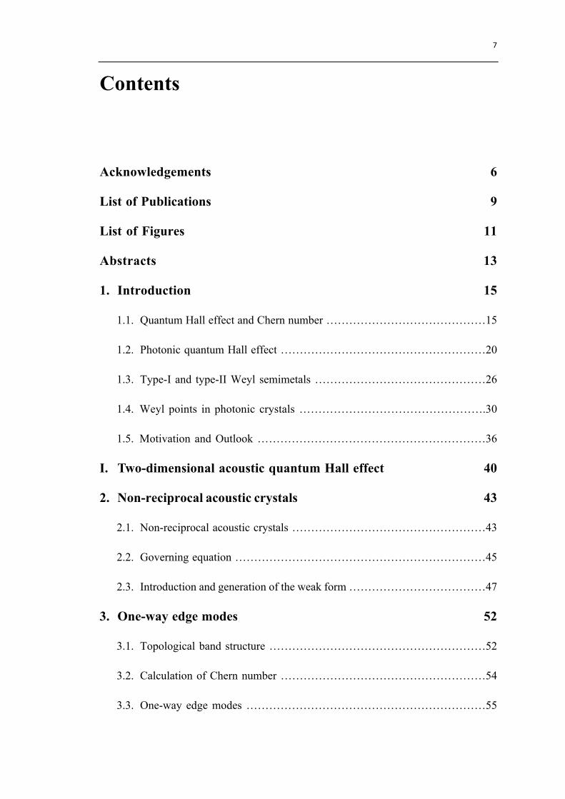
Contents

Acknowledgements 6

List of Publications 9

List of Figures 11

Abstracts 13

1. Introduction 15

1.1. Quantum Hall effect and Chern number ……………………………………15

1.2. Photonic quantum Hall effect ………………………………………………20

1.3. Type-I and type-II Weyl semimetals ………………………………………26

1.4. Weyl points in photonic crystals ………………………………………….30

1.5. Motivation and Outlook ……………………………………………………36

I. Two-dimensional acoustic quantum Hall effect 40

2. Non-reciprocal acoustic crystals 43

2.1. Non-reciprocal acoustic crystals ……………………………………………43

2.2. Governing equation …………………………………………………………45

2.3. Introduction and generation of the weak form ………………………………47

3. One-way edge modes 52

3.1. Topological band structure …………………………………………………52

3.2. Calculation of Chern number ………………………………………………54

3.3. One-way edge modes ………………………………………………………55

8

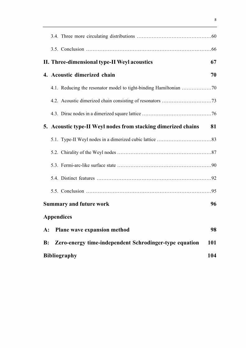
3.4. Three more circulating distributions ………………………………………60

3.5. Conclusion …………………………………………………………………66

II. Three-dimensional type-II Weyl acoustics 67

4. Acoustic dimerized chain 70

4.1. Reducing the resonator model to tight-binding Hamiltonian ………………70

4.2. Acoustic dimerized chain consisting of resonators …………………………73

4.3. Dirac nodes in a dimerized square lattice ……………………………………76

5. Acoustic type-II Weyl nodes from stacking dimerized chains 81

5.1. Type-II Weyl nodes in a dimerized cubic lattice ……………………………83

5.2. Chirality of the Weyl nodes …………………………………………………87

5.3. Fermi-arc-like surface state …………………………………………………90

5.4. Distinct features ……………………………………………………………92

5.5. Conclusion …………………………………………………………………95

Summary and future work 96

Appendices

A: Plane wave expansion method 98

B: Zero-energy time-independent Schrodinger-type equation 101

Bibliography 104

9

List of Publications First or corresponding author:

1. Z. Yang, F. Gao, X. Shi, X. Lin, Z. Gao, Y. Chong, B. Zhang. Topological acoustics.

Phys. Rev. Lett. 114, 114301 (2015).

2. Z. Yang, B. Zhang. Acoustic type-II Weyl nodes from stacking dimerized chains.

Phys. Rev. Lett. 117, 224301 (2016).

3. Z. Yang, F. Gao and B. Zhang, Topological water wave states in a one-dimensional

structure. Scientific Reports 6, 29202 (2016).

4. Z. Yang, F. Gao, X. Shi and B. Zhang. Synthetic-gauge-field-induced Dirac

semimetal state in an acoustic resonator system. New J. Phys. 18, 125003 (2016).

Invited paper: Focus on Topological Mechanics.

5. K. Shastri, Z. Yang*, B. Zhang*, Realizing type-II Weyl points in an optical lattice.

Phys. Rev. B 95, 014306 (2017).

6. Z. Yang, F. Gao, Y. Yang and B. Zhang. Strain-induced gauge field and Landau

levels in acoustic structures. Phys. Rev. Lett. 118, 194301 (2017).

7. Z. Yang, M. Xiao, F. Gao, L. Lu, Y. Chong and B. Zhang. Weyl points in a

magnetic tetrahedral photonic crystal. Optics Express 25, 15772-15777 (2017).

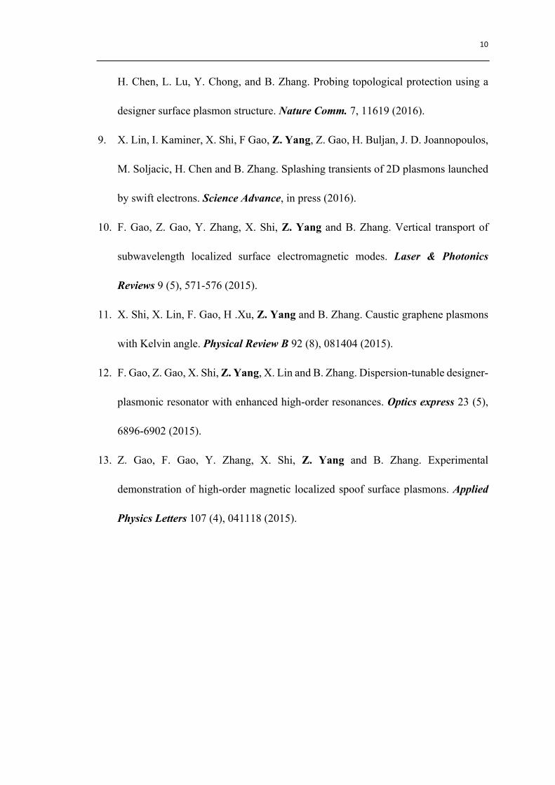
Co-authors:

8. Fei Gao, Z. Gao, X. Shi, Z. Yang, X. Lin, H. Xu, J. D. Joannopoulos, M. Soljacic,

10

H. Chen, L. Lu, Y. Chong, and B. Zhang. Probing topological protection using a

designer surface plasmon structure. Nature Comm. 7, 11619 (2016).

9. X. Lin, I. Kaminer, X. Shi, F Gao, Z. Yang, Z. Gao, H. Buljan, J. D. Joannopoulos,

M. Soljacic, H. Chen and B. Zhang. Splashing transients of 2D plasmons launched

by swift electrons. Science Advance, in press (2016).

10. F. Gao, Z. Gao, Y. Zhang, X. Shi, Z. Yang and B. Zhang. Vertical transport of

subwavelength localized surface electromagnetic modes. Laser & Photonics

Reviews 9 (5), 571-576 (2015).

11. X. Shi, X. Lin, F. Gao, H .Xu, Z. Yang and B. Zhang. Caustic graphene plasmons

with Kelvin angle. Physical Review B 92 (8), 081404 (2015).

12. F. Gao, Z. Gao, X. Shi, Z. Yang, X. Lin and B. Zhang. Dispersion-tunable designer-

plasmonic resonator with enhanced high-order resonances. Optics express 23 (5),

6896-6902 (2015).

13. Z. Gao, F. Gao, Y. Zhang, X. Shi, Z. Yang and B. Zhang. Experimental

demonstration of high-order magnetic localized spoof surface plasmons. Applied

Physics Letters 107 (4), 041118 (2015).

11

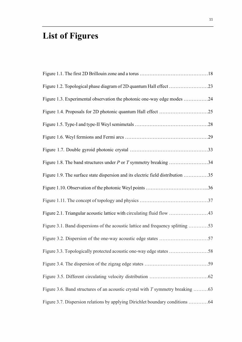
List of Figures

Figure 1.1. The first 2D Brillouin zone and a torus ……………………………………18

Figure 1.2. Topological phase diagram of 2D quantum Hall effect ……………………23

Figure 1.3. Experimental observation the photonic one-way edge modes ……………24

Figure 1.4. Proposals for 2D photonic quantum Hall effect …………………………25

Figure 1.5. Type-I and type-II Weyl semimetals ………………………………………28

Figure 1.6. Weyl fermions and Fermi arcs ……………………………………………29

Figure 1.7. Double gyroid photonic crystal …………………………………………33

Figure 1.8. The band structures under P or T symmetry breaking ……………………34

Figure 1.9. The surface state dispersion and its electric field distribution ……………35

Figure 1.10. Observation of the photonic Weyl points ………………………………...36

Figure 1.11. The concept of topology and physics ……………………………………37

Figure 2.1. Triangular acoustic lattice with circulating fluid flow ……………………43

Figure 3.1. Band dispersions of the acoustic lattice and frequency splitting …………53

Figure 3.2. Dispersion of the one-way acoustic edge states …………………………57

Figure 3.3. Topologically protected acoustic one-way edge states ……………………58

Figure 3.4. The dispersion of the zigzag edge states …………………………………59

Figure 3.5. Different circulating velocity distribution ………………………………62

Figure 3.6. Band structures of an acoustic crystal with T symmetry breaking ………63

Figure 3.7. Dispersion relations by applying Dirichlet boundary conditions …………64

12

Figure 3.8. Dispersion relations by applying hard boundary conditions ………………65

Figure 4.1. Acoustic dimerized chain and the band structures ………………………...72

Figure 4.2. Topological interface state ………………………………………………75

Figure 4.3. Acoustic 2D dimerized square lattice ……………………………………79

Figure 4.4. Flat edge states for the finite 2D lattice ……………………………………80

Figure 5.1. Acoustic Weyl nodes ……………………………………………………82

Figure 5.2. Acoustic 3D dimerized cubic lattice ………………………………………85

Figure 5.3. The band structures ………………………………………………………86

Figure 5.4. The distribution of type-II Weyl nodes ……………………………………89

Figure 5.5. Fermi-arc-like surface states ……………………………………………91

Figure 5.6. The distinct features ………………………………………………………94

13

Abstract

This thesis studies two classes of unconventional acoustic crystals.

The first class of the acoustic crystal is a two-dimensional crystal with

topologically gapped band structure. Circulating flow is introduced into each unit cell

to play the role of vector potential. We present a theoretical model to characterize the

underlying physics – quantum Hall effect for acoustics. Through numerical calculation,

we show that the nontrivial band gap emerges and the band below the gap acquires a

non-zero Chern number. As a result, the non-reciprocal acoustic crystal exhibits a

topologically protected one-way edge state inside the band gap.

The second class of the acoustic crystal is a three-dimensional and gapless crystal.

The isolated degenerate points, which are known as type-II Weyl nodes in three-

dimensional momentum space, indicate the existence of topological transition and

acquire non-zero Chern number. The Weyl nodes are rather robust against perturbations

and annihilate only in pairs of opposite chirality. In addition, the topological Fermi-arc-

like surface states can be traced out as an analogue of Fermi arcs as in condensed matter

physics. Last but not least, we demonstrate the unique features of the acoustic type-II

Weyl system, such as a finite density of states, transport properties of the surface states.

14

15

Chapter 1

Introduction

The Nobel Prize in Physics 2016 was divided, one half awarded to David J.

Thouless, the other half jointly to F. Duncan M. Haldane and J. Michael Kosterlitz "for

theoretical discoveries of topological phase transitions and topological phases of matter".

Their theoretical discoveries illustrate in a very nice way the interplay between

physics and mathematics. Here we will discuss the background of the topological phases

– quantum Hall effect and Weyl physics in condensed matter physics and photonics.

1.1 Quantum Hall effect and Chern number

The study of topological properties of band structures began with the discovery of

quantum Hall effect in 1980s [1]. The Hall conductance of the two-dimensional (2D)

electron gas in a magnetic field is an integer multiple of a constant 𝑒"/ℎ, which leads

to a fundamental question – what is the reason of the quantization of Hall conductance

independent of sample geometry. In the pioneering work [2], D. J. Thouless, 2016 Nobel

laureate in physics, and three other collaborators found the topological origin of Hall

conductance. The expression of Hall conductance in the unit 𝑒"/ℎ is a topological

invariant called Chern number or TKNN number, which is expressed as a winding

16

number of the Berry phase of electron wave functions around the Brillouin zone and

always an integer. This integer number characterizes the topological properties of the

wave functions in the band. In other words, within the scope of band theory, the insulator

with a band gap can be either an ordinary band insulator or a quantum Hall state. Once

one physical observable can be written as a topological invariant, it changes only

discretely. Therefore, it will not respond to continuous perturbations. This explains the

quantized values of Hall conductance.

Traditional phases of matter are classified by their different symmetries. However,

this classification method cannot be applied to the quantum Hall states. The pioneering

work of Thouless et al. offered us a new way to classify different phases of quantum

matter according to their topological order.

The non-zero Chern numbers are associated with various intriguing physical

phenomena. The most interesting property is the chiral edge states in quantum Hall

effect, or one-way edge modes in photonic crystals – waves travel in a single direction

along the edge without back-scattering, regardless of the existence of small

perturbations. Now I will present a review of the relevant mathematical background.

To learn the topological invariant, we start from introducing the band structure and

Bloch theorem. Generally, every crystal is an infinite and periodic structure that can be

characterized by a Bravais lattice, and for each Bravais lattice we can derive

the reciprocal lattice, which encapsulates the periodicity in three reciprocal vectors. The

periodic potential which shares the same periodicity as the lattice can be expanded out

as a Fourier series whose non-vanishing components are associated with the reciprocal

17

lattice vectors. From this theory, we can predict the band structure of a particular

material. For electrons in a perfect crystal, there is a basis of wavefunctions with the

properties: Each of these wavefunctions corresponds to an energy eigenstate. Each of

these wavefunctions is a Bloch wave, meaning that this wavefunction can be written in

the form: 𝜓 𝑟 = 𝑒()*𝑢(𝑟), where 𝑢 has the same periodicity as the atomic structure

of the crystal. This Bloch's theorem underlies the concept of band structures.

Now let us consider an insulator with N occupied bands defined by a crystal

Hamiltonian ℋ. The Bloch wave functions can be written as 𝜓/,) 𝑟 = 𝑒()*𝑢/,)(𝑟),

where k is the crystal momentum and n is the band index. Here 𝑢/,)(𝑟) obeys the

orthonormality condition and is cell-periodic eigen-function of the Bloch Hamiltonian

𝐻), which satisfies the relationship 𝐻)𝑢/,) = 𝐸/,)𝑢/,). Through Fourier transform, we

can derive the Bloch Hamiltonian in the k-momentum space from the original

Hamiltonian. The eigenvectors of the Bloch Hamiltonian give the Bloch waves.

For each band n, the Chern number [3, 4] is defined as

𝐶/ =12𝜋 𝑑𝑠 ∙ ℱ(𝑘)

(1.1)

where ℱ = 𝛻)×𝒜 is Berry curvature and 𝒜 = 𝑖 𝑢/,) 𝛻) 𝑢/,) is Berry

connection. The Eq. (1.1) is an area integral carried out in both momentum k space over

the first Brillouin zone and real space over the unit cell. Berry connection measures the

local change in the phase of wave-functions in momentum space. Similar to the vector

potential and Aharonov–Bohm phase, Berry connection and Berry phase 𝒜 ∙ 𝑑𝑙 are

gauge dependent, which means 𝑢/,) 𝑟 → 𝑒(B𝑢/,) 𝑟 , whereas the Berry curvature and

18

Chern number are gauge-invariant. The Berry phase is defined only up to multiples of

2𝜋. The inner product is performed in real space. The phase and flux can be connected

through Stokes’ theorem. The integral on a surface of the Berry curvature 𝛻)×𝒜, which

is also known as Chern density, is Berry flux. If the surface is a closed manifold, the

boundary integral vanishes. However the indeterminacy of the boundary term modulo of

2𝜋 manifests itself in the Chern theorem, which states that the integral of the Berry

curvature over a closed manifold is quantized in units of 2𝜋. This number is the Chern

number introduced above, and is essential for understanding various quantization effects.

The one-dimensional (1D) Berry phase is also known as the Zak phase [5].

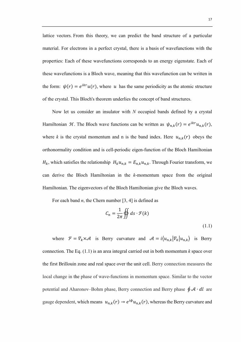
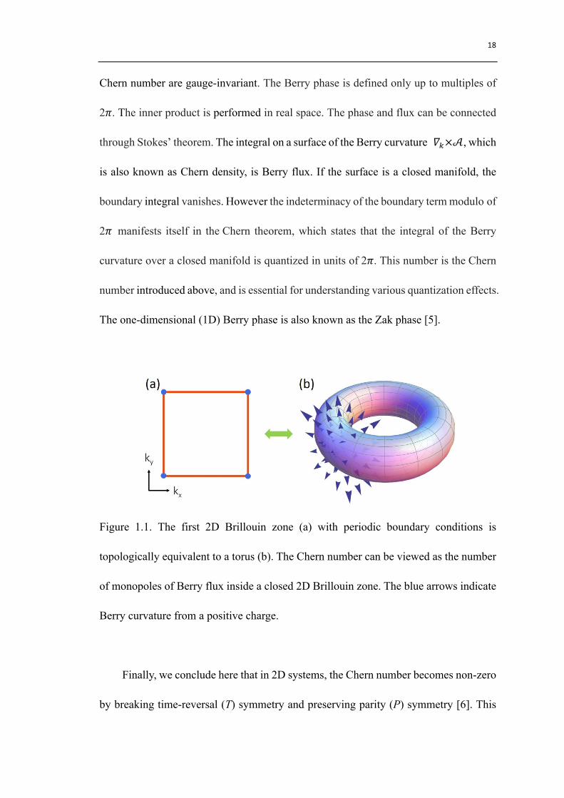
Figure 1.1. The first 2D Brillouin zone (a) with periodic boundary conditions is

topologically equivalent to a torus (b). The Chern number can be viewed as the number

of monopoles of Berry flux inside a closed 2D Brillouin zone. The blue arrows indicate

Berry curvature from a positive charge.

Finally, we conclude here that in 2D systems, the Chern number becomes non-zero

by breaking time-reversal (T) symmetry and preserving parity (P) symmetry [6]. This

19

2D quantum Hall topological phase with broken T symmetry in photonics will be the

focus at the next section. The Chern number is the integral of the Berry curvature over

the 2D first Brillouin zone with periodic boundary conditions. A torus is created if we

connect the two pair of periodic boundaries, which indicates the first Brillouin zone is

topologically equivalent to a torus as shown in Fig. 1.1. The Berry curvature is a pseudo-

vector field, which is odd under T but even under P. If we take Dirac cone, which is a

doubly degenerate point with linear dispersion, for elaboration, in presence of both P

and T, ℱ 𝑘 = 0. When either P or T symmetry is broken, the Dirac cones open and

each degeneracy-lifting term contributes a Berry flux of 𝜋 to each of the bulk bands.

In the presence of T (P broken), ℱ 𝑘 = −ℱ −𝑘 . The integration over the closed 2D

Brillouin zone is thus zero, which means the Chern number is zero. Whereas in the

presence of P (T broken), ℱ 𝑘 = ℱ −𝑘 . The total Berry flux will become 2𝜋 and

the Chern number equals one. Non-zero Chern number measures the number of

monopoles (topological charges) contained within the torus as schematically shown in

Fig. 1.1. In three-dimensional (3D) Brillouin zone, these charges are known as Weyl

points [7].

Last but not the least, in a finite 2D system, the non-zero Chern number gives

basically the relationship between the total number of edge states and the topological

properties of all the bulk bands below the gap. For example, if the Chern number is 1

for a band gap, there will be one unidirectional edge state spanning across the gap. This

is so called bulk-edge correspondence [3, 4].

20

1.2 Photonic quantum Hall effect

F. D. M. Haldane, 2016 Nobel laureate of physics, and S. Raghu proposed an

analog of integer quantum Hall effect in photonic crystals in 2005 [8]. In a remarkable

new direction, they predicted the existence of one-way electromagnetic modes similar

to the chiral edge states. These edge modes are confined at the edge of the 2D magneto-

optical photonic crystals. They acquire group velocities pointing in one direction, which

is determined by the direction of the applied dc magnetic field. Due to the lack of the

back-propagating modes, back-scattering is totally suppressed. This remarkable

property is potentially important for creating a range of new opportunities throughout

the photonic community.

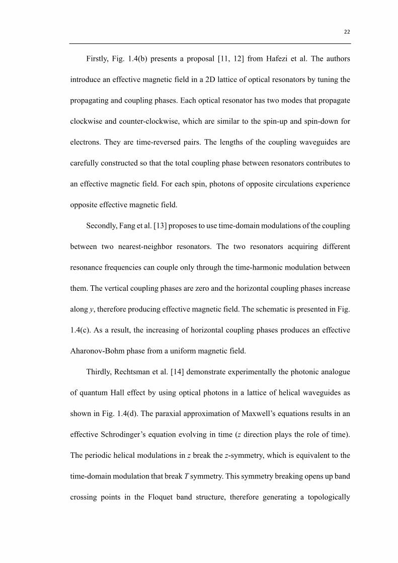
Figure 1.2 shows the topological phase diagram of the 2D quantum Hall effect [6].

The top-left panel shows a projected band structure of edge modes, in which the bulk

dispersions form a pair of Dirac points (shaded grey) protected by both P and T

symmetry. The green and blue lines represent the flat edge dispersions similar to

graphene on the opposite (top and bottom) edges. When either P or T is broken, a

bandgap can be generated in the bulk but not necessarily on the edges. When T

symmetry breaking is dominant, the two bulk bands split and acquire Chern numbers of

±1. Thus, there is one single gapless edge state localized on each of the top and bottom

edges, assuming the bulk is interfaced with topologically trivial insulators. This T-

breaking phase of non-zero Chern numbers is the 2D quantum Hall phase, plotted in red

21

in the right panel of the phase diagram.

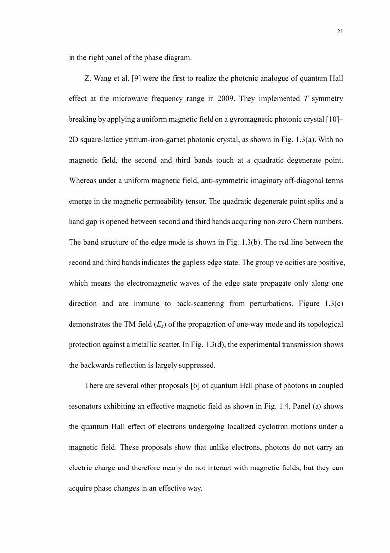
Z. Wang et al. [9] were the first to realize the photonic analogue of quantum Hall

effect at the microwave frequency range in 2009. They implemented T symmetry

breaking by applying a uniform magnetic field on a gyromagnetic photonic crystal [10]–

2D square-lattice yttrium-iron-garnet photonic crystal, as shown in Fig. 1.3(a). With no

magnetic field, the second and third bands touch at a quadratic degenerate point.

Whereas under a uniform magnetic field, anti-symmetric imaginary off-diagonal terms

emerge in the magnetic permeability tensor. The quadratic degenerate point splits and a

band gap is opened between second and third bands acquiring non-zero Chern numbers.

The band structure of the edge mode is shown in Fig. 1.3(b). The red line between the

second and third bands indicates the gapless edge state. The group velocities are positive,

which means the electromagnetic waves of the edge state propagate only along one

direction and are immune to back-scattering from perturbations. Figure 1.3(c)

demonstrates the TM field (Ez) of the propagation of one-way mode and its topological

protection against a metallic scatter. In Fig. 1.3(d), the experimental transmission shows

the backwards reflection is largely suppressed.

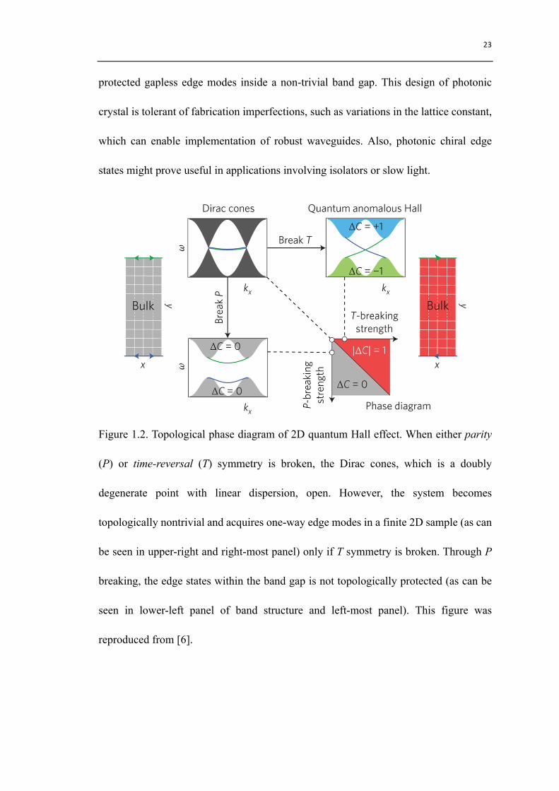
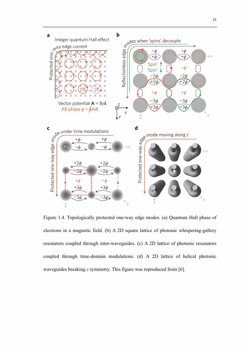
There are several other proposals [6] of quantum Hall phase of photons in coupled

resonators exhibiting an effective magnetic field as shown in Fig. 1.4. Panel (a) shows

the quantum Hall effect of electrons undergoing localized cyclotron motions under a

magnetic field. These proposals show that unlike electrons, photons do not carry an

electric charge and therefore nearly do not interact with magnetic fields, but they can

acquire phase changes in an effective way.

22

Firstly, Fig. 1.4(b) presents a proposal [11, 12] from Hafezi et al. The authors

introduce an effective magnetic field in a 2D lattice of optical resonators by tuning the

propagating and coupling phases. Each optical resonator has two modes that propagate

clockwise and counter-clockwise, which are similar to the spin-up and spin-down for

electrons. They are time-reversed pairs. The lengths of the coupling waveguides are

carefully constructed so that the total coupling phase between resonators contributes to

an effective magnetic field. For each spin, photons of opposite circulations experience

opposite effective magnetic field.

Secondly, Fang et al. [13] proposes to use time-domain modulations of the coupling

between two nearest-neighbor resonators. The two resonators acquiring different

resonance frequencies can couple only through the time-harmonic modulation between

them. The vertical coupling phases are zero and the horizontal coupling phases increase

along y, therefore producing effective magnetic field. The schematic is presented in Fig.

1.4(c). As a result, the increasing of horizontal coupling phases produces an effective

Aharonov-Bohm phase from a uniform magnetic field.

Thirdly, Rechtsman et al. [14] demonstrate experimentally the photonic analogue

of quantum Hall effect by using optical photons in a lattice of helical waveguides as

shown in Fig. 1.4(d). The paraxial approximation of Maxwell’s equations results in an

effective Schrodinger’s equation evolving in time (z direction plays the role of time).

The periodic helical modulations in z break the z-symmetry, which is equivalent to the

time-domain modulation that break T symmetry. This symmetry breaking opens up band

crossing points in the Floquet band structure, therefore generating a topologically

23

protected gapless edge modes inside a non-trivial band gap. This design of photonic

crystal is tolerant of fabrication imperfections, such as variations in the lattice constant,

which can enable implementation of robust waveguides. Also, photonic chiral edge

states might prove useful in applications involving isolators or slow light.

Figure 1.2. Topological phase diagram of 2D quantum Hall effect. When either parity

(P) or time-reversal (T) symmetry is broken, the Dirac cones, which is a doubly

degenerate point with linear dispersion, open. However, the system becomes

topologically nontrivial and acquires one-way edge modes in a finite 2D sample (as can

be seen in upper-right and right-most panel) only if T symmetry is broken. Through P

breaking, the edge states within the band gap is not topologically protected (as can be

seen in lower-left panel of band structure and left-most panel). This figure was

reproduced from [6].

24

Figure 1.3. (a) Experimental set-up. (b) Band structure of the edge modes. (c) Simulation

field of the one-way edge mode and its topological protection against a scatter. (d) First

measured topologically protected transmission of the edge modes at microwave

frequency. This figure was reproduced from [6, 9].

25

Figure 1.4. Topologically protected one-way edge modes. (a) Quantum Hall phase of

electrons in a magnetic field. (b) A 2D square lattice of photonic whispering-gallery

resonators coupled through inter-waveguides. (c) A 2D lattice of photonic resonators

coupled through time-domain modulations. (d) A 2D lattice of helical photonic

waveguides breaking z symmetry. This figure was reproduced from [6].

26

1.3 Type-I and type-II Weyl semimetals

Weyl semimetals [15] that host isolated Weyl points in 3D momentum space have

been discovered in the material TaAs [16, 17] and a double-gyroid photonic crystal [18],

as a new topological phase of matter beyond topological insulators. The novel Weyl

materials exhibit unusual physical properties such as open Fermi arcs [15] and chiral

anomaly [19]. The new Weyl physics has drawn immediate attention in condensed

matter physics as well as in photonics.

The dispersion of Weyl points is governed by the Weyl Hamiltonian [7]

𝐻 𝑘 = 𝑘(𝑣(G𝜎G(,GIJ,K,L ,

(1.2)

where 𝑣(G and 𝜎G are group velocity and Pauli matrix, respectively. The existence of

Weyl points is possible only if either P or T is broken and stable to weak perturbations

[6, 20]. When a Weyl point is present in the 3D momentum space, it can be viewed as a

topological charge – either a source or a sink of Berry curvature. The Fermi surface

enclosing a Weyl point has a well-defined Chern number, which indicates the

topological charge of this Weyl point. Due to the fact that the net charge must vanish in

the Brillouin zone, Weyl points come up in pairs. They are stable and annihilated only

in pairs of opposite chirality.

However, Soluyanov et al. recently proposed the existence of a previously missed

type of Weyl fermion – Lorentz-violating type-II Weyl fermion [21], that emerges at the

boundary between electron and hole pockets in a new phase of matter. It was overlooked

27

by Weyl because it breaks stringent Lorentz symmetry in high-energy physics. Because

Lorentz invariance does not need to be respected in condensed matter physics,

Soluyanov et al. found the new type of Weyl fermion by generalizing the Dirac equation.

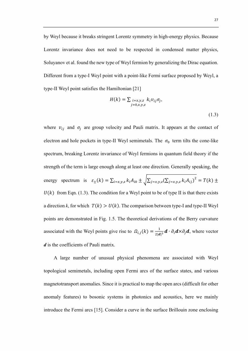
Different from a type-I Weyl point with a point-like Fermi surface proposed by Weyl, a

type-II Weyl point satisfies the Hamiltonian [21]

𝐻 𝑘 = 𝑘(𝑣(G𝜎G(IJ,K,LGIM,J,K,L

,

(1.3)

where 𝑣(G and 𝜎G are group velocity and Pauli matrix. It appears at the contact of

electron and hole pockets in type-II Weyl semimetals. The 𝜎M term tilts the cone-like

spectrum, breaking Lorentz invariance of Weyl fermions in quantum field theory if the

strength of the term is large enough along at least one direction. Generally speaking, the

energy spectrum is 𝜀± 𝑘 = 𝑘(𝐴(M(IJ,K,L ± ( 𝑘(𝐴(G)GIJ,K,L"

GIJ,K,L = 𝑇(𝑘) ±

𝑈(𝑘) from Eqn. (1.3). The condition for a Weyl point to be of type II is that there exists

a direction k, for which 𝑇 𝑘 > 𝑈 𝑘 . The comparison between type-I and type-II Weyl

points are demonstrated in Fig. 1.5. The theoretical derivations of the Berry curvature

associated with the Weyl points give rise to 𝛺(,G(𝑘) =T

"|𝒅|W𝒅 ∙ 𝜕(𝒅×𝜕G𝒅, where vector

d is the coefficients of Pauli matrix.

A large number of unusual physical phenomena are associated with Weyl

topological semimetals, including open Fermi arcs of the surface states, and various

magnetotransport anomalies. Since it is practical to map the open arcs (difficult for other

anomaly features) to bosonic systems in photonics and acoustics, here we mainly

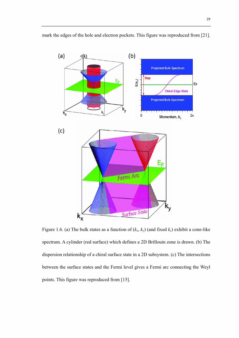
introduce the Fermi arcs [15]. Consider a curve in the surface Brillouin zone enclosing

28

the projection of the Weyl point, which is traversed anti-clockwise as varying the

parameter 𝜆:0 − 2𝜋 (𝑘\ ), as shown in Fig. 1.6(a). The 𝑘\ and 𝑘L define the 2D

surface Brillouin zone, which is topologically equivalent to a torus. Therefore the Chern

number of the 2D Brillouin zone simply corresponds to the net monopole enclosed

within the torus. Consider a single enclosed Weyl point, the 2D system defined in the

2D surface Brillouin zone can be viewed as a quantum Hall state with Chern number 1.

For a finite 2D subsystem with a boundary, a chiral edge state is expected for the sub-

2D system, as presented in Fig. 1.6(b). Consequently, each surface state crosses the zero

energy (Fermi surface for simplicity) somewhere on the 2D surface Brillouin zone. Thus,

at the zero energy, there is a Fermi line terminates at the Weyl points in the 2D surface

Brillouin zone as demonstrated in Fig. 1.6(c). We also note that an arc starting at a Weyl

point of one chirality must terminate at a Weyl point of the opposite chirality. This open

arc is later well known as the “Fermi arc”.

Figure 1.5. Possible types of Weyl semimetals. (a) Type-I Weyl point with a point-like

Fermi surface. (b) Type-II Weyl point appears at the contact of electron and hole pockets.

The grey plane corresponds to the position of the Fermi surface. The blue and red lines

29

mark the edges of the hole and electron pockets. This figure was reproduced from [21].

Figure 1.6. (a) The bulk states as a function of (kx, ky) (and fixed kz) exhibit a cone-like

spectrum. A cylinder (red surface) which defines a 2D Brillouin zone is drawn. (b) The

dispersion relationship of a chiral surface state in a 2D subsystem. (c) The intersections

between the surface states and the Fermi level gives a Fermi arc connecting the Weyl

points. This figure was reproduced from [15].

30

1.4 Weyl points in photonic crystals

The first proposal of Weyl photonics has been manifested in a double-gyroid

photonic crystal [20] as shown in Fig. 1.7. Panel (a) shows the cubic unit cell of length

a. Panel (b) presents the crystal in a primitive unit cell of space group 230. Consisting

of triple junctions in a body-centered cubic lattice, the gyroid surface is approximated

by iso-surfaces [20, 22] of

𝑔 𝑟 = 𝑠𝑖𝑛 2𝜋𝑥 𝑎 𝑐𝑜𝑠 2𝜋𝑦 𝑎 + 𝑠𝑖𝑛 2𝜋𝑦 𝑎 𝑐𝑜𝑠 2𝜋𝑧 𝑎 +

𝑠𝑖𝑛 2𝜋𝑧 𝑎 𝑐𝑜𝑠 2𝜋𝑥 𝑎 ,

(1.4)

where a is the lattice constant. The double-gyroid photonic crystal are made of the two

separate 3D regions enclosed by two single gyroid surfaces:

𝑔 𝑟 > 1.1 and 𝑔 −𝑟 > 1.1.

(1.5)

The scheme of P symmetry or T symmetry breaking lifts the threefold degeneracy

at the center of the 3D Brillouin zone and leads to the different pairs of Weyl points as

shown in Fig. 1.8, which are annihilated only in pairs of opposite charge. Band structures

of single-gyroid and double gyroid photonic crystal are shown in Fig. 1.8(a).

In absence of P symmetry, the T symmetry is preserved and maps a Weyl point at

momentum k to its inversion point –k with the same chirality, there exist two other Weyl

points of opposite chirality. The P symmetry is broken by putting one air sphere on one

of the gyroids at the middle point of the two neighboring triple junctions shown in Fig.

31

1.7 (b). As presented in Fig. 1.8(b), under the P symmetry breaking perturbation, there

are two pairs of Weyl points appearing along 𝛤𝛨 and 𝛤𝑁. It should be mentioned that,

there is no other state near the Weyl points’ frequency.

When T symmetry is absent but P symmetry is preserved. By applying d.c.

magnetic field along 𝛤𝛨 (y direction) to the double-gyroid photonic crystal as shown

in Fig. 1.7 (a) to break T symmetry, the high-index double-gyroid material is assumed

to become gyro-electric and the permittivity tensor is now

𝜀(|𝐵|) =𝜀TT(|𝐵|) 0 𝑖𝜀T"(|𝐵|)

0 𝜀 0−𝑖𝜀T"(|𝐵|) 0 𝜀TT(|𝐵|)

,

(1.6)

where 𝜀 = 16, and 𝑑𝑒𝑡 𝜀(|𝐵|) = (𝜀TT"(|𝐵|) − 𝜀T""(|𝐵|))𝜀 = 𝜀m. Note that 𝜀T" is a

non-zero real number when the magnetization is present. The dimensionless effective

magnetic field intensity is defined as 𝐵 = 𝜀T" 𝜀. As presented in Fig. 1.8(c), under

the T symmetry breaking perturbation, there is only a single pair of Weyl points

appearing along the magnetization direction. The reason is that P symmetry maps a

Weyl point at momentum k to –k with opposite chirality.

As a result of non-zero Chern number, there are topologically protected gapless

chiral surface state inside the band gap away from the Weyl points. Figure 1.9 shows the

surface dispersion under P breaking perturbation along a line cut in the 2D surface

Brillouin zone with non-zero Chern number. The red line indicates the existence of one-

way chiral surface states. The lower panel of Fig. 1.9 demonstrates the electric field

intensity of the surface state. We can easily see that the electric fields are mostly

confined at the surface between topologically trivial (single gyroid) and non-trivial

32

(double gyroid) photonic crystals.

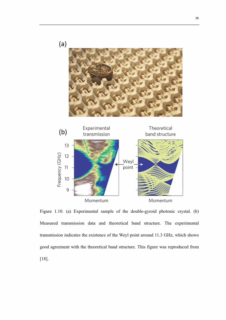
Two years after the theoretical proposal in 2013, Lu et al. experimentally observed

the Weyl points [18] in a double-gyroid photonic crystal with P-symmetry-breaking

perturbation in the micro-wave frequency range. The experimental sample is shown in

Fig. 1.10(a). The measured transmission data in Fig. 1.10(b) verifies the existence of

Weyl points predicated from theoretical proposal. Recently the robust surface states in

a metallic-hexagonal photonic crystal were experimentally observed [23]. Besides the

previous experimental observations, Noh et al. [24] has reported the measurement of the

type-II Weyl points in a lattice of helical waveguides in optical frequency range.

The rich physics of Weyl points has drawn intense interests in Weyl photonic

systems [18, 20, 23-29]. The Weyl points of photonics share almost the same topological

properties as in condensed matter physics. At the Weyl-point frequencies, photonic Weyl

materials provide angular selectivity for filtering light from any 3D incident angle. The

unique density of states at the Weyl point can potentially enable devices such as high-

power single-mode lasers.

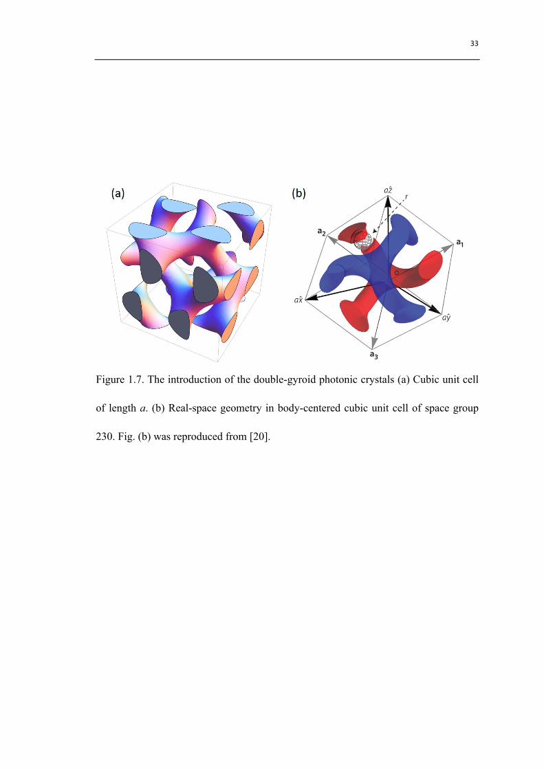
33

Figure 1.7. The introduction of the double-gyroid photonic crystals (a) Cubic unit cell

of length a. (b) Real-space geometry in body-centered cubic unit cell of space group

230. Fig. (b) was reproduced from [20].

34

Figure 1.8. The existence of Weyl points in double-gyroid photonic crystals with P-

breaking and T-breaking perturbations, respectively. (a) Band structures of single-gyroid

and double gyroid photonic crystal. There are triply degenerate points with quadratic

dispersion relationship. (b) The band structure of double-gyroid photonic crystal under

P-breaking perturbation. (c) The band structure under T symmetry breaking with

magnetization along 𝛤𝛨. The right insets show the distribution of different paired Weyl

points in the Brillouin zone. This figure was reproduced from [20].

35

Figure 1.9. The surface dispersion under P symmetry breaking only along a line cut in

a 2D surface Brillouin zone with non-zero Chern number and enclosing unpaired Weyl

points. The dispersion of the surface state acquires only negative group velocity within

the band gap. The bottom panel demonstrates the electric field intensity of the surface

state. Clearly we can see that the electric field is localized at the interface between the

topologically trivial and non-trivial crystals. This figure was reproduced from [20].

36

Figure 1.10. (a) Experimental sample of the double-gyroid photonic crystal. (b)

Measured transmission data and theoretical band structure. The experimental

transmission indicates the existence of the Weyl point around 11.3 GHz, which shows

good agreement with the theoretical band structure. This figure was reproduced from

[18].

37

1.5 Motivation and Outlook

Acoustic waves in fluids has many applications in our daily life, including medical

imaging, acoustic sonar etc. Acoustic technologies frequently develop using shared

concepts with optics such as crystal and meta-media. The sonic crystals and acoustic

metamaterial developed in the last two decades may have novel applications in acoustic

isolators, super-lens, cloaking etc. It is thus valuable to introduce new concepts like

topology into the system to explore the topological manipulations of acoustic waves.

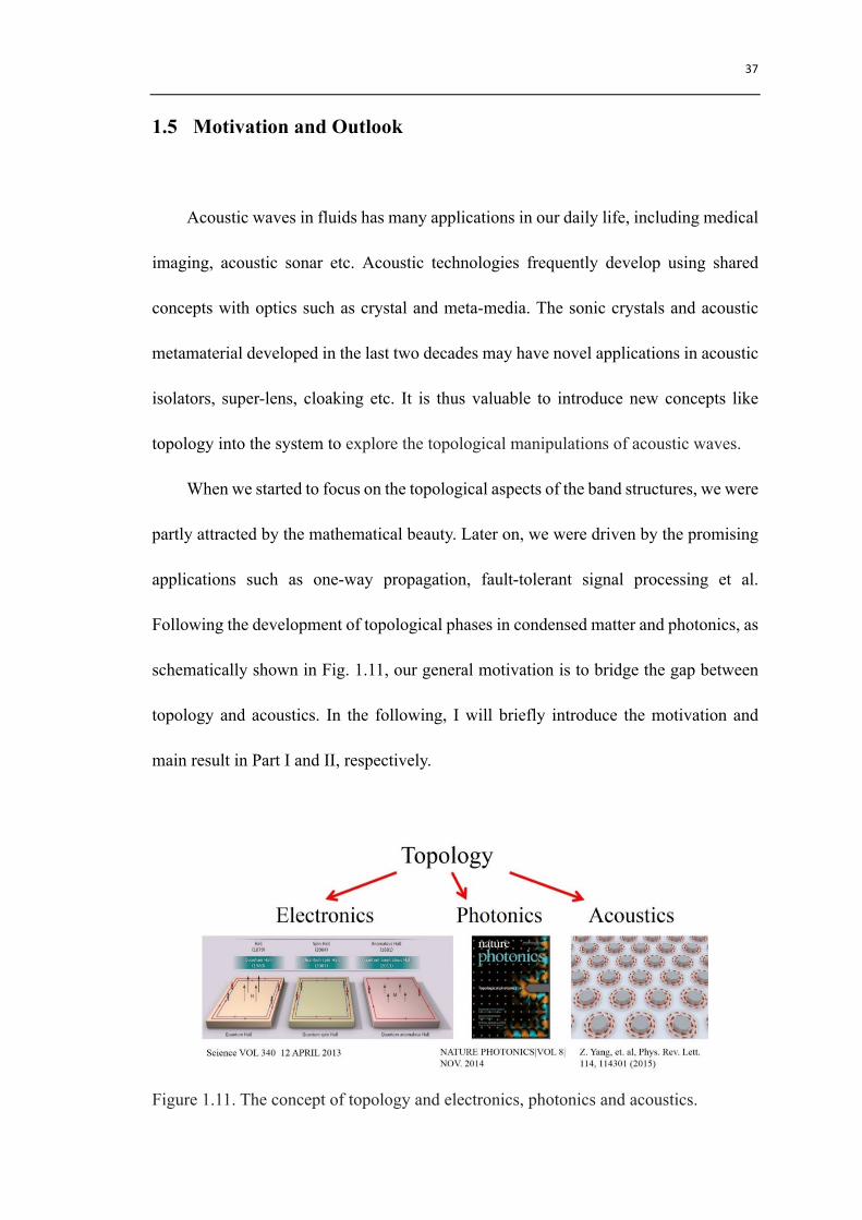
When we started to focus on the topological aspects of the band structures, we were

partly attracted by the mathematical beauty. Later on, we were driven by the promising

applications such as one-way propagation, fault-tolerant signal processing et al.

Following the development of topological phases in condensed matter and photonics, as

schematically shown in Fig. 1.11, our general motivation is to bridge the gap between

topology and acoustics. In the following, I will briefly introduce the motivation and

main result in Part I and II, respectively.

Figure 1.11. The concept of topology and electronics, photonics and acoustics.

38

First, based on the previous introductions, we can see the concept of topology has

been introduced into electronic and photonic systems. Therefore, an open question

remains elusive, whether the concept of topology can be implemented in the traditional

acoustic systems. In Part I, we will show that for the first time we map the quantum Hall

effect into an acoustic crystal by introducing circulating flow.

Second, as the observation of the type-I Weyl points in the condensed matter TaAs

and a double-gyroid photonic crystal, Weyl physics has drawn intense attention.

However, the newly developed Lorentz-violating type-II Weyl fermions, which are

missed in Weyl’s original prediction, still stay isolated from bosonic systems such as

photonics and acoustics. In Part II, we propose a 3D acoustic crystal hosting type-II

Weyl points. A structure is constructed, in a simple way, from stacking 1D building

blocks – dimerized chains.

It is valuable to explore the topological manipulations of acoustic waves, given the

promising applications of topological states in electronic and photonic systems (such as

fault-tolerant quantum computations, optical multiplexing, et al.). For instance, sound

waves are guided in a single direction around the surface of a region and ignore

imperfections that would scatter the sound in an ordinary material. If it can be realized,

such a system may find applications in many acoustic technologies, such as one-way

waveguides, soundproofing and sonar stealth systems.

The field of topological insulators is now developing rapidly in condensed matter

physics as well as in bosonic systems, such as photonics [6, 27, 30-40], acoustics [41,

39

42] and mechanics [43].

40

Part I

Two-dimensional acoustic quantum Hall effect

41

The manipulation of acoustic waves in fluids has tremendous applications,

including those in everyday life. Acoustic technologies have frequently developed in

tandem with optics, using shared concepts such as wave-guiding and meta-media. It is

thus noteworthy that an entirely novel class of topological edge states in a photonic

quantum Hall state, has recently been demonstrated. Haldane (one of the winners of

2016 Nobel laureates in physics) and Raghu predicted that a similar phenomenon can

arise in the context of classical electromagnetism, which was subsequently bourne out

by experiments on microwave-scale magneto-optic photonic crystals and other photonic

devices. These are inspired by electronic edge states occurring in topological insulators,

and possess a promising property – the ability to propagate in a single direction along

an edge without back-scattering, regardless of the defects or disorder.

Here in Part I, we first develop a theoretical model of 2D topological acoustics [44],

and propose a scheme for realizing topological edge states in a non-reciprocal acoustic

structure containing circulating fluids as shown in Chapter 2. The property of

topologically protected one-way acoustic wave propagation is demonstrated in Chapter

3, which does not occur in ordinary acoustic devices and may have novel applications

for acoustic isolators, modulators and transducers.

42

43

Chapter 2

Non-reciprocal acoustic crystals

2.1 Non-reciprocal acoustic crystals

Acoustic wave in fluid is an oscillatory motion with small amplitude in a

compressible fluid [45, 46]. It has no intrinsic spin and does not respond to magnetic

fields and its reciprocal transmission is directly associated to the symmetry of physics

laws under time reversal, which in other word indicates the lack of unidirectional control.

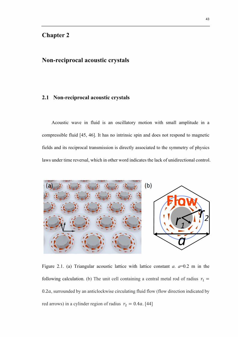
Figure 2.1. (a) Triangular acoustic lattice with lattice constant a. a=0.2 m in the

following calculation. (b) The unit cell containing a central metal rod of radius 𝑟T =

0.2𝑎, surrounded by an anticlockwise circulating fluid flow (flow direction indicated by

red arrows) in a cylinder region of radius 𝑟" = 0.4𝑎. [44]

44

In order to realize topological band theory in acoustics, we begin with a spatially

periodic medium, and introduce a mechanism that breaks T symmetry. A periodic

acoustic medium, sometimes called a ‘phononic crystal’ [47], is commonly realized by

engineering a structure whose acoustic properties (elastic moduli and/or mass density)

vary periodically on a scale comparable to the acoustic wavelength. As for T symmetry

breaking, although traditional acoustic devices lack an efficient mechanism to

accomplish this propose, a recent breakthrough [48] has shown that strong T-breaking

can be achieved in a ‘meta-atom’ containing a ring of circulating fluid. Although these

developments have direct device applications as acoustic diode [49] and acoustic

circulator [48], they do not have the topological protection against defects possessed by

the topological edge states. We utilize the design concept by incorporating circulating

fluid elements into an acoustic crystal structure. As shall be seen later, the resulting

acoustic band structure is topologically nontrivial, supports the non-reciprocal

propagations of acoustic waves and maps theoretically onto an integer quantum Hall gas

– the simplest version of a 2D topological insulator.

The proposed acoustic structure is shown in Fig. 2.1(a). Fig. 2.1(b) shows the unit

cell with circulating air flow. It is a triangular lattice of lattice constant a, where each

unit cell consists of a rigid solid cylinder (e.g. a metal cylinder) with radius r1,

surrounded by a cylindrical rotating-fluid-filled region of radius r2. The rest of the unit

cell with radius bigger than r2 consists of a stationary fluid, separated from the fluid in

the cylindrical region by a thin impedance-matched layer at radius r2. (This layer can be

45

achieved using a thin sheet of solid material that is permeable to sound) The central

cylinder rotates along its axis with angular speed 𝛺, which produces a circulatory flow

in the surrounding fluid. (We will not consider the possibility of vortexes like Taylor

vortex [45] caused by large 𝛺 in experiment because we here focus on 2D model and

Taylor vortex does not contribute an effective flux through x-y plane.) We assume that

fluid velocity is much slower than the speed of sound (Mach number, which is defined

as 𝑣/𝑐, is less than 0.3). The motion of the fluid can be described by a circulating

‘Couette flow’ distribution [45]; the velocity field points in the azimuthal direction, with

component 𝑣o = − p*qr

*rrs*qr𝑟 + p*qr*rr

*rrs*qrT*, where r is measured from the origin at the axis of

the cylinder. This angular velocity is equal to 𝛺 at radius r=r1, and zero at radius r=r2.

2.2 Governing equation

In the previously designed non-reciprocal acoustic crystal, the propagation of

sound waves in the presence of such a steady-state non-homogenous velocity

background is described in Refs. [50-52]. Assuming that the viscosity and heat flow are

negligible, we can start from three independent equations – Euler, continuity and state

equations in terms of acoustic disturbances of 𝑝, 𝜌 and 𝑣: 𝜌M𝜕v𝑣 + ∇𝑝 = 0, 𝜕v𝜌 +

𝜌M∇ ∙ 𝑣 = 0 and 𝑝 = 𝑐M"𝜌. Derived from the above three equations, we can arrive at the

sound master equation:

Tx𝛻 ∙ 𝜌𝛻𝜙 − 𝜕v + 𝑣M ∙ 𝛻

Tzr

𝜕v + 𝑣M ∙ 𝛻 𝜙 = 0,

46

(2.1)

where 𝜌 is the fluid density, 𝑐 is the speed of sound, and 𝑣M is the background fluid

velocity.

The relation between velocity potential 𝜙 and sound pressure p is 𝑝 = 𝜌(𝜕v + 𝑣M ∙

𝛻)𝜙. We take the surface of each cylinder as an impenetrable hard boundary by setting

𝑛 ∙ 𝛻𝜙 = 0 where 𝑛 is the surface normal vector.

It should be mentioned that, the Eq. (2.1) is a linearized-approximated equation.

The latter simulation results may have small deviations if we adopt other wave models

as recently shown in Ref. [53, 54]. However, the physical results are robust and reliable.

We can explore the above differential equation analytically through the plane wave

expansion method and obtain the effective Hamiltonian in vicinity of the high symmetry

points K (K’) at the corners of the Brillouin zone. The details of the mathematical

manipulation can be found in Appendix A. Without circulating flow, the dispersion of

the two lowest bands at the corners of the Brillouin zone exhibits the Dirac cone

spectrum. However, when the circulating air flow in each unit cell is introduced, band

gap opens because of the T symmetry breaking.

We restrict our attention to time-harmonic solutions with frequency 𝜔 and neglect

second order terms as 𝑣M 𝑐 " ≪ 1. With a change of variables 𝛹 = 𝜌𝜙 the master

equation can be rewritten as [10]

(𝛻 − 𝑖𝐴~��)" + 𝑉(𝑥, 𝑦) 𝛹 = 0,

(2.2)

where the effective vector and scalar potentials are

47

𝐴~�� = −𝜔𝑣M(𝑥, 𝑦)

𝑐"

𝑉 𝑥, 𝑦 = − T�𝛻 𝑙𝑛 𝜌 " − T

"𝛻" 𝑙𝑛 𝜌 + �r

zr.

Evidently Eq. (2.2) maps onto the Schrodinger equation for a spin-less charged quantum

particle in non-uniform vector and scalar potentials. The details of the derivation can be

found in the Appendix B. For non-zero 𝛺, the inner boundary of the Couette flow

contributes positive effective magnetic flux, and the rest of the Couette flow contributes

negative effective magnetic flux; the net magnetic flux, integrated over the entire unit

cell, is zero. The acoustic system thus behaves like a ‘zero field quantum Hall’ system

[55] and is periodic in the unit cell.

It is worth mentioning that a similar approach to construct an effective magnetic

vector potential for classical wave propagation has been discussed by Berry and

colleagues [56]. These authors showed that an irrotational (‘bathtub’) fluid votex

exhibits a classical wavefront dislocation effect, analogous to the Aharanov-Bohm

effect [57]. Here we advance this insight by applying the flow model to an acoustic

crystal context, so that the effective magnetic vector potential gives rise to a

topologically nontrivial acoustic band structure.

2.3 Introduction and generation of the weak form

Apart from exploring Eq. (2.1) analytically as shown in Appendix A and analyzing

the physical pictures qualitatively, we need to quantitatively characterize the physical

48

properties of the acoustic crystal we introduced in section 2.1. To solve the complex Eq.

(2.1) numerically, we can resort to the finite element method – commercial software

COMSOL Multiphysics, weak form PDE (physics interfaces). In general, the

commercial software collects all the equations and boundary conditions formulated by

the physics interfaces into a large system of partial derivative equations and boundary

conditions. COMSOL Multiphysics then solves the system by using a weak formulation.

The mathematical weak form can give us direct access to the terms of the weak equation

and provide maximum freedom in defining finite element problems. Therefore, I

provide a theoretical background to the weak form in COMSOL Multiphysics [58] in

this section and generate the weak form for our acoustic model.

First, I show a simple example – the conversion of a general formula to the weak

form. Consider a partial derivative equation with a single dependent variable, 𝑢, in two

space dimensions:

𝛻 ∙ 𝛤 = 𝐹, in domain 𝛺.

(2.3)

The functions 𝛤 and 𝐹 in general may be functions of both the dependent variable 𝑢

itself and its time derivative. Now let 𝑣 be an arbitrary function on 𝛺, and call it the

test function (𝑣 should of course belong to a suitably chosen well-behaved class of

functions, 𝑉 ). Multiplying the partial derivative equation with this function and

integrating leads to

𝑣𝛻 ∙ 𝛤𝑑𝐴p = 𝑣𝐹𝑑𝐴p ,

(2.4)

49

where 𝑑𝐴 is the area element. We can use Gauss’ formula to integrate by parts and

arrive at

𝑣𝛤 ∙ 𝑛𝑑𝑠�p − 𝛻𝑣 ∙ 𝛤𝑑𝐴p = 𝑣𝐹𝑑𝐴p .

(2.5)

where 𝑑𝑠 is the length element. Therefore when we apply the Neumann boundary

condition:

−𝑛 ∙ 𝛤 = 𝐺 + ����𝜇,

(2.6)

we can obtain the equation below:

0 = 𝛻𝑣 ∙ 𝛤 + 𝑣𝐹 𝑑𝐴 + 𝑣(𝐺 + ����𝜇)𝑑𝑠�pp .

(2.7)

Together with the Dirichlet condition, this is a weak reformulation of the original partial

derivative equation problem. The requirement shows that the previous weak formula

should hold for all test functions 𝑣. One can reverse the steps of the derivation to show

that if the functions 𝑢 and 𝜇 satisfy the weak formula, then they also satisfy the

original formula. However, this holds true only if the solutions and coefficients are

smooth enough. For example, in the case of discontinuities in material properties, one

can have a solution of the weak formulation, however the strong formula then has no

sense. The names weak and strong come from the difference: the weak formulation is a

weaker condition on the solution than the strong formula. An advantage of this weak

formulation is that it needs less regularity of 𝛤. This is vital in the finite element method.

By introducing the boundary conditions on the test functions

50

𝑣 ����= 0, on 𝜕𝛺.

(2.8)

Then the weak reformulation becomes the following function

0 = 𝛻𝑣 ∙ 𝛤 + 𝑣𝐹 𝑑𝐴p + 𝑣𝐺𝑑𝑠�p0 = 𝑅�𝑜𝑛𝑏𝑜𝑢𝑛𝑑𝑎𝑟𝑦𝜕𝛺

.

(2.9)

The Eq. (2.9) holds true for all test function 𝑣 meeting the boundary condition. Such a

formula arises if one have a variational principle. For example, to find the function 𝑢

that minimizes the energy of a physical system on the condition of the constraints 0 =

𝑅�. If the energy is given like an integral of an expression involving the function 𝑢,

thus the stationarity condition on the solution is accurately the weak formula as shown

above. Because variational principles are more fundamental than the corresponding

partial derivative equation, the weak form is often more natural than the strong forms.

After the introduction of the weak form in COMSOL Multiphysics, we try to

convert our acoustic Eq. (2.1) to a weak formula. Later on, we use the commercial

software to simulate the acoustic crystal and numerically calculate the dispersions and

acoustic pressure fields.

Following the similar path shown above, we start from Eq. (2.1) and apply the

Gauss’ formula. Finally, the weak reformulation of the Eq. (2.1) is

0 =

𝑑𝐴[−𝜌 ∗ ( 𝜕v,v𝑢 + 𝜕J𝑣 ∗ 𝜕J,v𝑢 + 𝜕K𝑣 ∗ 𝜕K,v𝑢 ∗𝑡𝑒𝑠𝑡 𝑢𝑐M"

+

𝑡𝑒𝑠𝑡 𝜕J𝑢 ∗ 𝜕J𝑢 − 𝜕v𝑢 + 𝜕J𝑣 ∗ 𝜕J𝑢 + 𝜕K𝑣 ∗ 𝜕K𝑢 ∗𝜕J𝑣𝑐M"

+

𝑡𝑒𝑠𝑡(𝜕K𝑢) ∗ (𝜕K𝑢 − (𝜕v𝑢 + 𝜕J𝑣 ∗ 𝜕J𝑢 + 𝜕K𝑣 ∗ 𝜕K𝑢) ∗𝜕K𝑣𝑐M"))]

p

51

(2.10)

where 𝑢 means the test function and 𝜕( indicates the derivative of a function with

respect to 𝑖 , where 𝑖 = 𝑥, 𝑦, 𝑡 . Several boundary conditions for different physical

characterizations correspond to different weak form on the boundaries. For example,

Floquet (periodic) boundary condition is used to calculate the band structures. Sound

hard boundary and scattering boundary condition are applied to mimic the physical

experiment for topologically protected edge states.

In the next Chapter, we technically import the Eq. (2.10) into the COMSOL

Multiphysics (the weak form physics interface), choose different boundaries and

numerically calculate the results.

52

Chapter 3

One-way edge modes

3.1 Topological band structure

We can calculate the acoustic band structures by using the finite-element

commercial software COMSOL Multiphysics. For simplicity, we assume the

background fluid involved is air. The results, with 𝛺 = 0 and 𝛺 ≠ 0, are shown in Fig.

3.1(a). For 𝛺 = 0 [red curves in Fig. 3.1(a)], the acoustic band structure exhibits a pair

of Dirac points at the corner of the hexagonal Brillouin zone, at frequency 𝜔M =

0.577×2𝜋𝑐�/𝑎 (992 Hz), where 𝑐� is the sound velocity in air.

For 𝛺 ≠ 0 the circulating air flow produces a dramatic change in the band

structure [blue curves in Fig. 3.1(a)]. Here, we set the angular velocity of the inner rods

to be 𝛺 = 2𝜋×400𝑟𝑎𝑑/𝑠 (which means 400 resolutions per second, achievable with

miniature electric motors). The Dirac point degeneracies are lifted, producing a finite

complete bandgap. The frequency splitting at the zone corners as a function of 𝛺, is

plotted in Fig. 3.1(b). The ratio of the operating frequency to the bandgap, which is an

estimate for the penetration depth of the topological edge states in units of the lattice

constant, is on the order of 𝜔/𝛿𝜔 ≈ 10 for the range of angular velocities plotted here.

53

Figure 3.1. (a) Band structures of the acoustic lattice without the circulating fluid flow

(red curves; 𝛺 = 2𝜋×0𝑟𝑎𝑑/𝑠) and with fluid flow (blue curves; 𝛺 = 2𝜋×400𝑟𝑎𝑑/

𝑠). In the gapped band structure, the bands have Chern number 1± (blue labels). Left

inset: enlarged view of Dirac cone. Right lower inset: the first Brillouin zone. (b)

Frequency splitting as a function of the angular velocity of the cylinder in each unit cell.

The degeneracy at the Dirac point with frequency 𝜔M = 0.577×2𝜋𝑐�/𝑎 (992 Hz) is

removed for 𝛺 ≠ 0. [44]

54

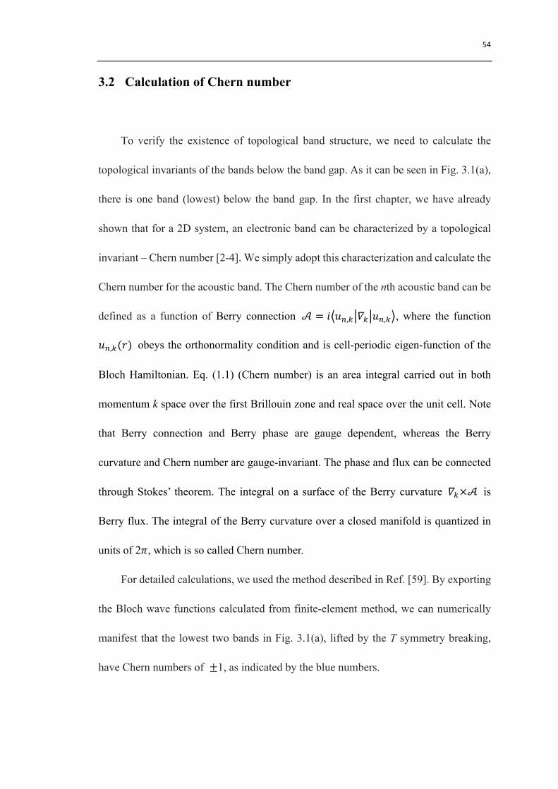
3.2 Calculation of Chern number

To verify the existence of topological band structure, we need to calculate the

topological invariants of the bands below the band gap. As it can be seen in Fig. 3.1(a),

there is one band (lowest) below the band gap. In the first chapter, we have already

shown that for a 2D system, an electronic band can be characterized by a topological

invariant – Chern number [2-4]. We simply adopt this characterization and calculate the

Chern number for the acoustic band. The Chern number of the nth acoustic band can be

defined as a function of Berry connection 𝒜 = 𝑖 𝑢/,) 𝛻) 𝑢/,) , where the function

𝑢/,)(𝑟) obeys the orthonormality condition and is cell-periodic eigen-function of the

Bloch Hamiltonian. Eq. (1.1) (Chern number) is an area integral carried out in both

momentum k space over the first Brillouin zone and real space over the unit cell. Note

that Berry connection and Berry phase are gauge dependent, whereas the Berry

curvature and Chern number are gauge-invariant. The phase and flux can be connected

through Stokes’ theorem. The integral on a surface of the Berry curvature 𝛻)×𝒜 is

Berry flux. The integral of the Berry curvature over a closed manifold is quantized in

units of 2𝜋, which is so called Chern number.

For detailed calculations, we used the method described in Ref. [59]. By exporting

the Bloch wave functions calculated from finite-element method, we can numerically

manifest that the lowest two bands in Fig. 3.1(a), lifted by the T symmetry breaking,

have Chern numbers of ±1, as indicated by the blue numbers.

55

3.3 One-way edge modes

The principle of bulk-edge correspondence [60] then predicts that, for a finite

acoustic crystal, the gap between these two bands is spanned by unidirectional acoustic

edge states, analogous to the electronic edge states occurring in the quantum Hall effect.

To confirm the existence of these topologically-protected acoustic edge states, we

numerically calculate the band structure for a 20×1 super-cell [61] (a ribbon that is 20-

unit-cell wide in y direction and infinite along x direction). As shown in Fig. 3.2(a), for

𝛺 = 2𝜋×400𝑟𝑎𝑑/𝑠 the bandgap contains two sets of edge states, which are confined

to opposite edges of the ribbon and have opposite group velocities.

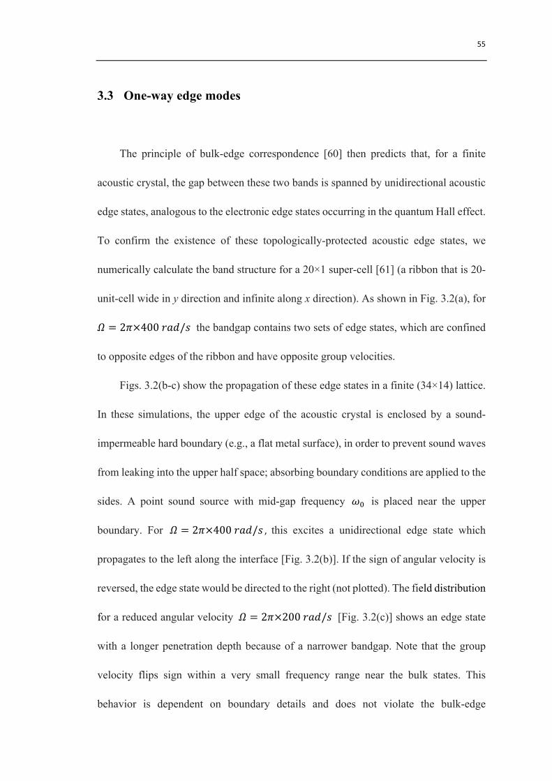
Figs. 3.2(b-c) show the propagation of these edge states in a finite (34×14) lattice.

In these simulations, the upper edge of the acoustic crystal is enclosed by a sound-

impermeable hard boundary (e.g., a flat metal surface), in order to prevent sound waves

from leaking into the upper half space; absorbing boundary conditions are applied to the

sides. A point sound source with mid-gap frequency 𝜔M is placed near the upper

boundary. For 𝛺 = 2𝜋×400𝑟𝑎𝑑/𝑠 , this excites a unidirectional edge state which

propagates to the left along the interface [Fig. 3.2(b)]. If the sign of angular velocity is

reversed, the edge state would be directed to the right (not plotted). The field distribution

for a reduced angular velocity 𝛺 = 2𝜋×200𝑟𝑎𝑑/𝑠 [Fig. 3.2(c)] shows an edge state

with a longer penetration depth because of a narrower bandgap. Note that the group

velocity flips sign within a very small frequency range near the bulk states. This

behavior is dependent on boundary details and does not violate the bulk-edge

56

correspondence principle.

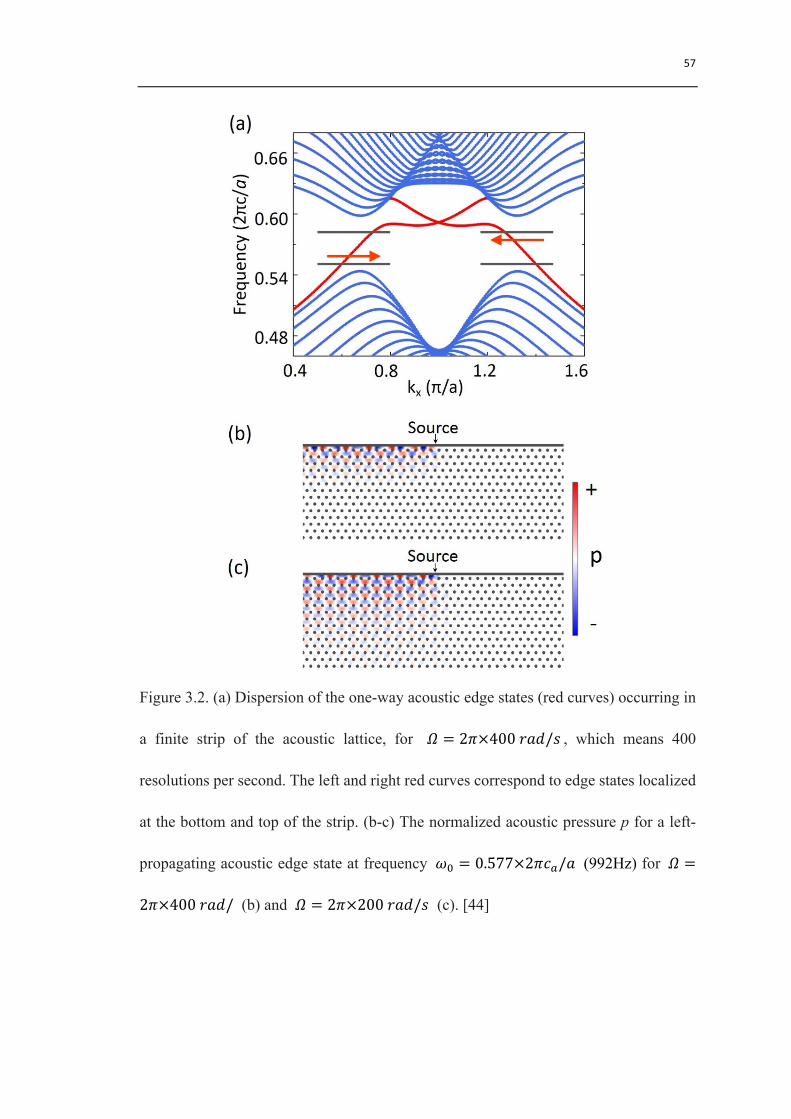
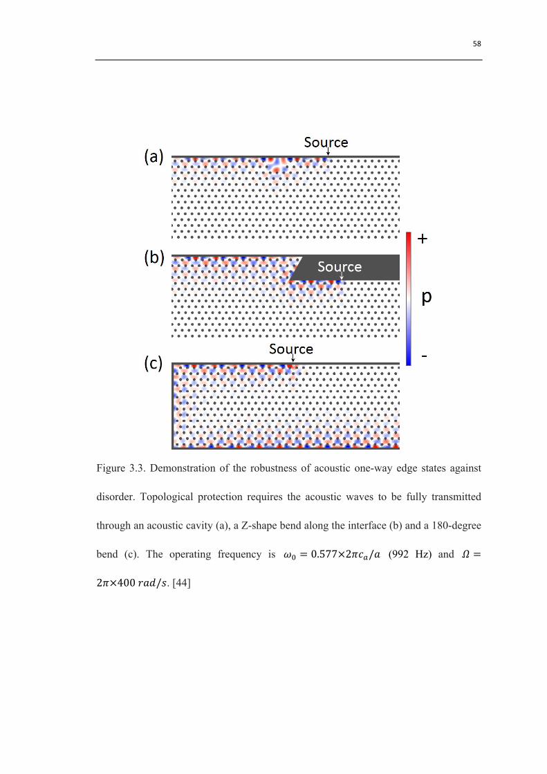
Due to the lack of backward-propagating edge modes, the presence of disorder

cannot cause backscattering. Fig. 3.3(a) shows an acoustic cavity located along the

interface; the incident wave flows through the cavity, and excites localized resonances

within the cavity, but does not backscatter. Fig. 3.3(b) shows a Z-shape bend connecting

two parallel surfaces at different y; again, the acoustic edge states are fully transmitted

across the bend. Finally, Fig. 2.5(c) shows a 180-degree bend which allows acoustic

edge states to be guided from the top of

the sample to the bottom of the sample. Note that the top and bottom boundaries are

called ‘zigzag’ shape boundaries. Whereas the left boundary in this sample is an

‘armchair’ boundary, which supports one-way edge states with different dispersion

relations.

In addition, we numerically calculate the dispersion relation of a 20×1 super-cell

(a ribbon that is 20-unit-cell wide in x direction and infinite along y direction). In this

case, the armchair shape of the edges can still support the topologically protected one-

way surface modes, as shown in Fig. 3.4(a). For 𝛺 = 2𝜋×400𝑟𝑎𝑑/𝑠 , within the

bandgap there are two edge states corresponding to right and left edges of the ribbon,

which have positive and negative group velocities, respectively. The schematic in Fig.

3.4(b) shows the propagation style of the edge states shown in panel (a).

57

Figure 3.2. (a) Dispersion of the one-way acoustic edge states (red curves) occurring in

a finite strip of the acoustic lattice, for 𝛺 = 2𝜋×400𝑟𝑎𝑑/𝑠 , which means 400

resolutions per second. The left and right red curves correspond to edge states localized

at the bottom and top of the strip. (b-c) The normalized acoustic pressure p for a left-

propagating acoustic edge state at frequency 𝜔M = 0.577×2𝜋𝑐�/𝑎 (992Hz) for 𝛺 =

2𝜋×400𝑟𝑎𝑑/ (b) and 𝛺 = 2𝜋×200𝑟𝑎𝑑/𝑠 (c). [44]

58

Figure 3.3. Demonstration of the robustness of acoustic one-way edge states against

disorder. Topological protection requires the acoustic waves to be fully transmitted

through an acoustic cavity (a), a Z-shape bend along the interface (b) and a 180-degree

bend (c). The operating frequency is 𝜔M = 0.577×2𝜋𝑐�/𝑎 (992 Hz) and 𝛺 =

2𝜋×400𝑟𝑎𝑑/𝑠. [44]

59

Figure 3.4. (a) The dispersion of the edge states projected along x direction. Note that in

Fig. 3.2, the band structure projects along y direction. There are two edge states

propagating along one direction corresponding to opposite edges. (b) The schematic

shows the propagation style of the edge states shown in panel (a).

60

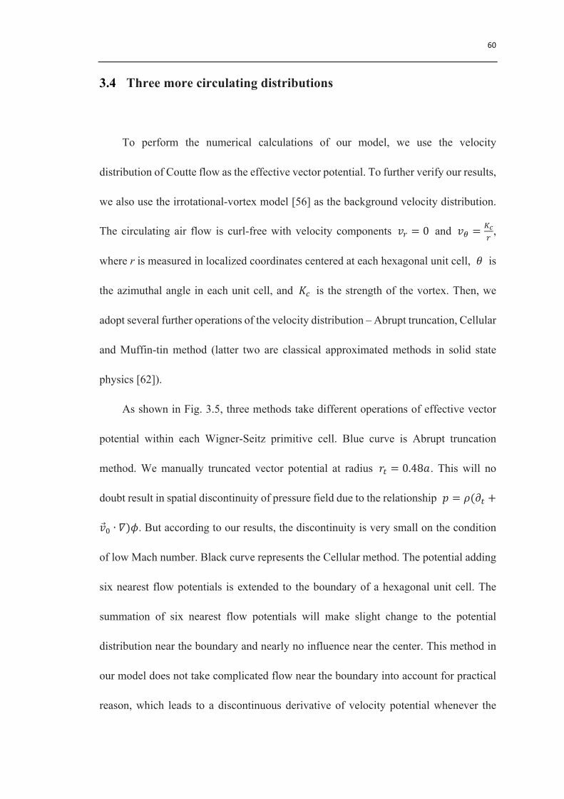
3.4 Three more circulating distributions

To perform the numerical calculations of our model, we use the velocity

distribution of Coutte flow as the effective vector potential. To further verify our results,

we also use the irrotational-vortex model [56] as the background velocity distribution.

The circulating air flow is curl-free with velocity components 𝑣* = 0 and 𝑣o =��*

,

where r is measured in localized coordinates centered at each hexagonal unit cell, 𝜃 is

the azimuthal angle in each unit cell, and 𝐾z is the strength of the vortex. Then, we

adopt several further operations of the velocity distribution – Abrupt truncation, Cellular

and Muffin-tin method (latter two are classical approximated methods in solid state

physics [62]).

As shown in Fig. 3.5, three methods take different operations of effective vector

potential within each Wigner-Seitz primitive cell. Blue curve is Abrupt truncation

method. We manually truncated vector potential at radius 𝑟v = 0.48𝑎. This will no

doubt result in spatial discontinuity of pressure field due to the relationship 𝑝 = 𝜌(𝜕v +

𝑣M ∙ 𝛻)𝜙. But according to our results, the discontinuity is very small on the condition

of low Mach number. Black curve represents the Cellular method. The potential adding

six nearest flow potentials is extended to the boundary of a hexagonal unit cell. The

summation of six nearest flow potentials will make slight change to the potential

distribution near the boundary and nearly no influence near the center. This method in

our model does not take complicated flow near the boundary into account for practical

reason, which leads to a discontinuous derivative of velocity potential whenever the

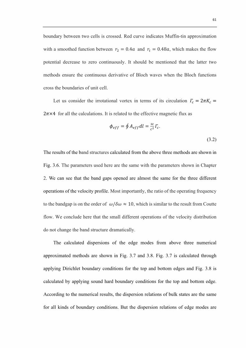
61

boundary between two cells is crossed. Red curve indicates Muffin-tin approximation

with a smoothed function between 𝑟" = 0.4𝑎 and 𝑟v = 0.48𝑎, which makes the flow

potential decrease to zero continuously. It should be mentioned that the latter two

methods ensure the continuous derivative of Bloch waves when the Bloch functions

cross the boundaries of unit cell.

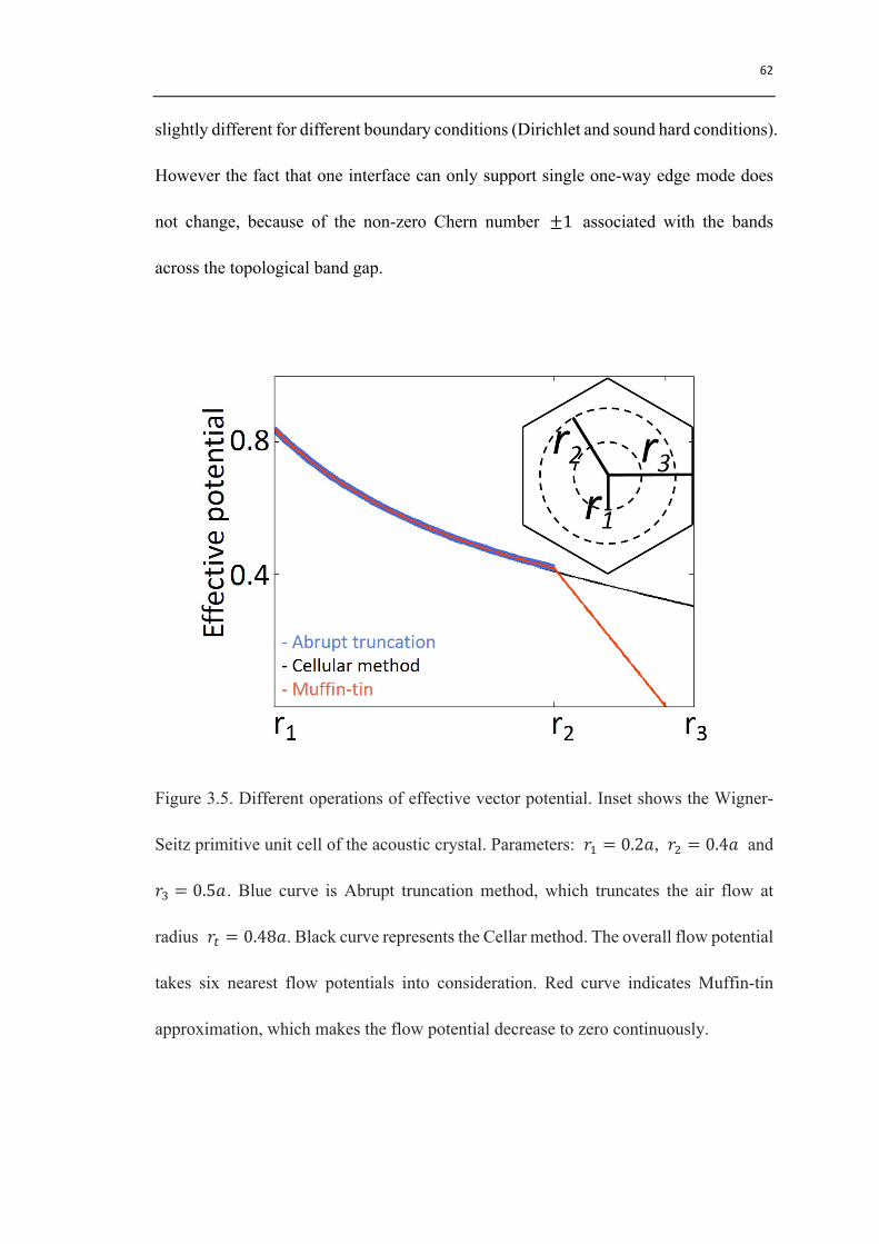
Let us consider the irrotational vortex in terms of its circulation 𝛤z = 2𝜋𝐾z =

2𝜋×4 for all the calculations. It is related to the effective magnetic flux as

𝜙~�� = 𝐴~��𝑑𝑙 =�zr𝛤z.

(3.2)

The results of the band structures calculated from the above three methods are shown in

Fig. 3.6. The parameters used here are the same with the parameters shown in Chapter

2. We can see that the band gaps opened are almost the same for the three different

operations of the velocity profile. Most importantly, the ratio of the operating frequency

to the bandgap is on the order of 𝜔/𝛿𝜔 ≈ 10, which is similar to the result from Coutte

flow. We conclude here that the small different operations of the velocity distribution

do not change the band structure dramatically.

The calculated dispersions of the edge modes from above three numerical

approximated methods are shown in Fig. 3.7 and 3.8. Fig. 3.7 is calculated through

applying Dirichlet boundary conditions for the top and bottom edges and Fig. 3.8 is

calculated by applying sound hard boundary conditions for the top and bottom edge.

According to the numerical results, the dispersion relations of bulk states are the same

for all kinds of boundary conditions. But the dispersion relations of edge modes are

62

slightly different for different boundary conditions (Dirichlet and sound hard conditions).

However the fact that one interface can only support single one-way edge mode does

not change, because of the non-zero Chern number ±1 associated with the bands

across the topological band gap.

Figure 3.5. Different operations of effective vector potential. Inset shows the Wigner-

Seitz primitive unit cell of the acoustic crystal. Parameters: 𝑟T = 0.2𝑎, 𝑟" = 0.4𝑎 and

𝑟m = 0.5𝑎. Blue curve is Abrupt truncation method, which truncates the air flow at

radius 𝑟v = 0.48𝑎. Black curve represents the Cellar method. The overall flow potential

takes six nearest flow potentials into consideration. Red curve indicates Muffin-tin

approximation, which makes the flow potential decrease to zero continuously.

63

Figure 3.6. Band structures of an acoustic crystal with T symmetry breaking. The

degeneracy of Dirac points at the corners of the Brillouin zone is lifted. The results of

the three numerical methods show good agreements with each other. Blue, black and

red curves correspond to Abrupt truncation method, Cellar method and Muffin-tin

approximation, respectively.

64

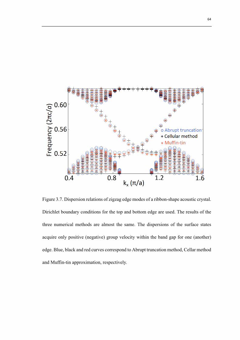
Figure 3.7. Dispersion relations of zigzag edge modes of a ribbon-shape acoustic crystal.

Dirichlet boundary conditions for the top and bottom edge are used. The results of the

three numerical methods are almost the same. The dispersions of the surface states

acquire only positive (negative) group velocity within the band gap for one (another)

edge. Blue, black and red curves correspond to Abrupt truncation method, Cellar method

and Muffin-tin approximation, respectively.

65

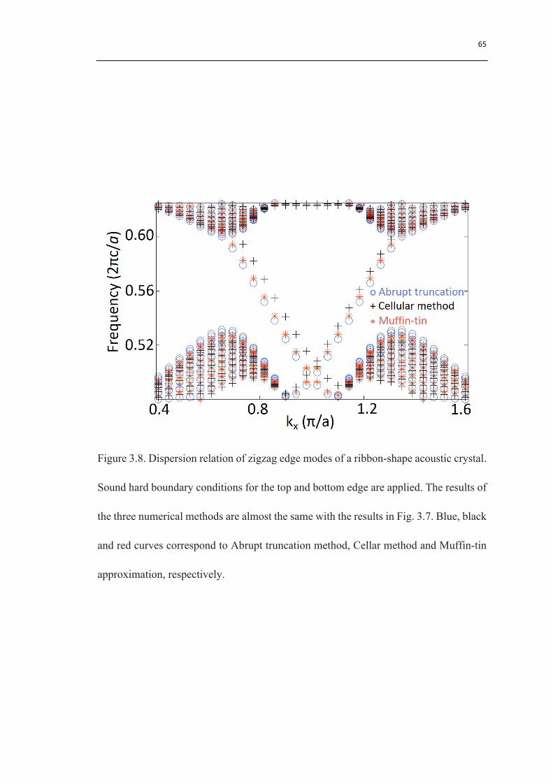
Figure 3.8. Dispersion relation of zigzag edge modes of a ribbon-shape acoustic crystal.

Sound hard boundary conditions for the top and bottom edge are applied. The results of

the three numerical methods are almost the same with the results in Fig. 3.7. Blue, black

and red curves correspond to Abrupt truncation method, Cellar method and Muffin-tin

approximation, respectively.

66

3.5 Conclusion

In conclusion, we numerically calculate topological band structure and the

dispersions of the edge states in the non-reciprocal acoustic crystal. We also demonstrate

the presence of topologically protected one-way acoustic edge states.

We need to point out that similar effects can be achieved with alternative designs

featuring circulatory fluid velocity distributions; e.g., having azimuthally-directed fans

in each unit cell [48], or stirring with a rotating disc on the top plate [52]. The effect

could be tunable in frequency ranges by appropriately scaling down lattice constant or

practically operating at higher band gaps with larger Chern numbers. Acoustic devices

based on these topological properties may be useful for invisibility from sonar detection,

one-way signal processing regardless of disorders, acoustic isolator, which will greatly

broaden our interest in military, medical and industrial applications.

We also want to point out that several groups have reported topological vibrational

modes in mechanical lattices [43, 63-68]. The present acoustic system, by contrast,

involves acoustic waves in continuous fluid media, which is considerably more relevant

for the existing acoustic technologies.

67

Part II

Three-dimensional type-II Weyl acoustics

68

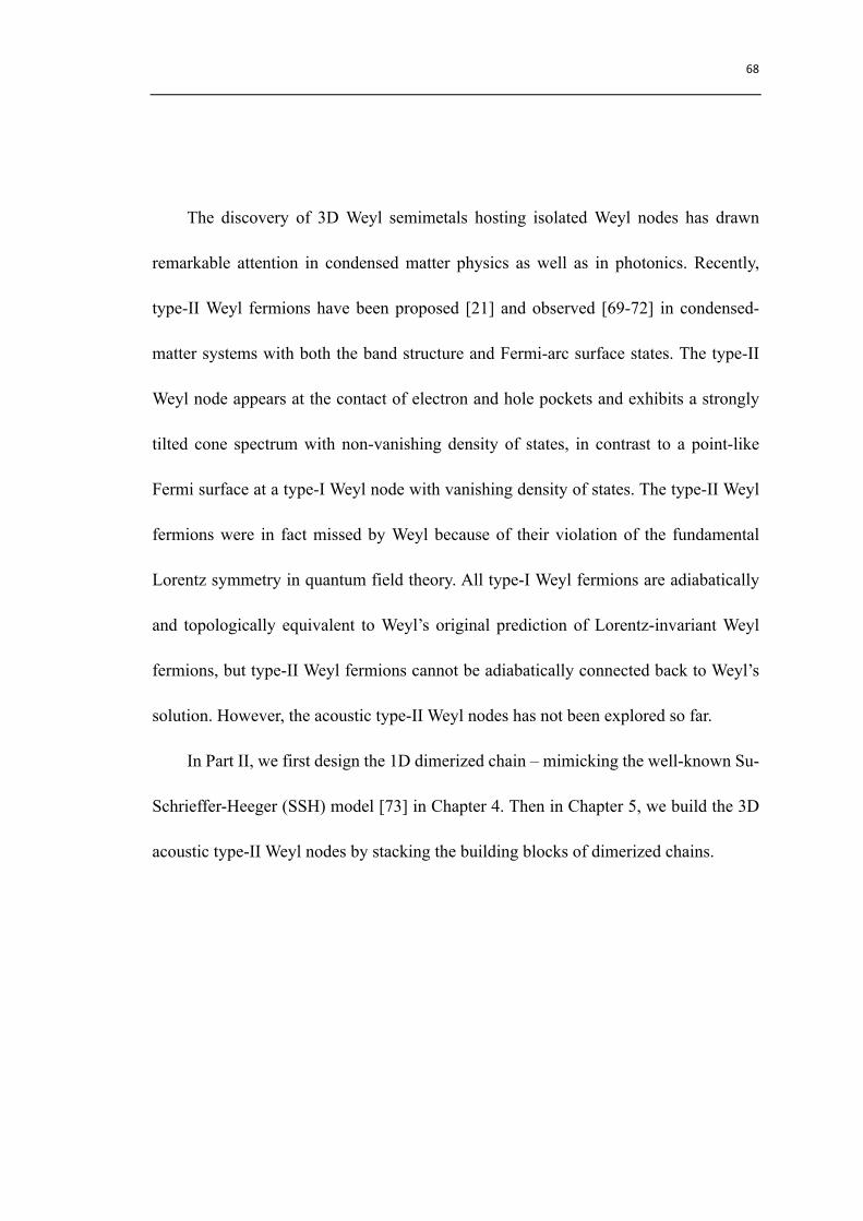
The discovery of 3D Weyl semimetals hosting isolated Weyl nodes has drawn

remarkable attention in condensed matter physics as well as in photonics. Recently,

type-II Weyl fermions have been proposed [21] and observed [69-72] in condensed-

matter systems with both the band structure and Fermi-arc surface states. The type-II

Weyl node appears at the contact of electron and hole pockets and exhibits a strongly

tilted cone spectrum with non-vanishing density of states, in contrast to a point-like

Fermi surface at a type-I Weyl node with vanishing density of states. The type-II Weyl

fermions were in fact missed by Weyl because of their violation of the fundamental

Lorentz symmetry in quantum field theory. All type-I Weyl fermions are adiabatically

and topologically equivalent to Weyl’s original prediction of Lorentz-invariant Weyl

fermions, but type-II Weyl fermions cannot be adiabatically connected back to Weyl’s

solution. However, the acoustic type-II Weyl nodes has not been explored so far.

In Part II, we first design the 1D dimerized chain – mimicking the well-known Su-

Schrieffer-Heeger (SSH) model [73] in Chapter 4. Then in Chapter 5, we build the 3D

acoustic type-II Weyl nodes by stacking the building blocks of dimerized chains.

69

70

Chapter 4

Acoustic dimerized chain

Note that a 1D acoustic topological phase has been realized in a 1D phononic

crystal [74], but not with resonators. Therefore, it cannot be precisely described by the

SSH tight-binding model due to the presence of long-range couplings. It is thus

interesting to investigate if a 1D chain consisting of resonators, each of which supports

a single-resonance mode, can realize 1D acoustic topological phase corresponding to

SSH model.

4.1 Reducing the resonator model to tight-binding Hamiltonian

In the section, we start with constructing a simple 1D tight-binding model which

consists of acoustic resonators only coupled to its nearest-neighboring resonator through

one coupling waveguide. Generally, this method can be extended to 2D and 3D acoustic

resonator systems, which will be directly applied in the next Chapter

Assuming there is an infinitely long 1D resonator chain as shown schematically in

the upper panel of Fig. 4.1(a) – two resonators per unit cell. The filled (open) circle

indicates A (B) type resonator. The lth resonator mode satisfies the following coupled-

mode equations [11, 14, 61]:

71

𝑖𝜕v𝑎� = 𝜅T𝑏���� and 𝑖𝜕v𝑏� = 𝜅"𝑎���� ,

(4.1)

where 𝑎 (b ) is the amplitude of resonator mode for type A (B) resonator. The

summation <m> is taken over the nearest-neighbor resonator. The hopping strength can

be obtained from above coupled-mode equations as 𝜅T = −𝜔/ 𝑏�|𝑎� 𝑑𝑉 and 𝜅" =

−𝜔/ 𝑎��T|𝑏� 𝑑𝑉 , where the integration is taken over the volume of the coupling

waveguide. The above coupled-mode equations can be viewed as a tight-binding

eigenvalue problem 𝐻𝜓 = 𝐸𝜓.

In particular, for the two-band model of 1D acoustic dimerized chain, the

construction is shown in lower panel of Fig. 4.1(a). The left and right nearest-neighbor

(NN) hopping strengths of A type resonator are 𝑡 + 𝛿𝑡 and 𝑡 − 𝛿𝑡, respectively. The

dispersion from coupled-mode equations is the same as the Hamiltonian 𝐻 =

[ 𝑡 + 𝛿𝑡 𝑎� 𝑏� + 𝑡 − 𝛿𝑡 𝑏�

 𝑎��T + ℎ. 𝑐. ]� , where 𝑎 ( 𝑏 ) and 𝑎  ( 𝑏  ) are the

annihilation and creation operators on the sub-lattice sites, 𝑡 and 𝛿𝑡 are the nearest

hopping and the tuning strength. They can be tuned by changing the radius (equivalently

changes V) of the cylindrical coupling waveguide. Furthermore we transfer the

Hamiltonian into k-space by performing Fourier transformation and setting zero energy

offset between two sites, we can arrive at the SSH model and obtain the Bloch

Hamiltonian H(k) for the 1D acoustic resonator system:

𝐻T 𝑘 = 2𝑡𝑐𝑜𝑠 𝑘J𝑎 𝜎J − 2𝛿𝑡𝑠𝑖𝑛(𝑘J𝑎)𝜎K.

(4.2)

72

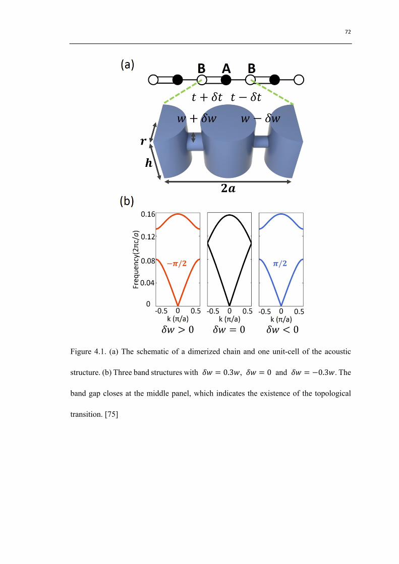
Figure 4.1. (a) The schematic of a dimerized chain and one unit-cell of the acoustic

structure. (b) Three band structures with 𝛿𝑤 = 0.3𝑤, 𝛿𝑤 = 0 and 𝛿𝑤 = −0.3𝑤. The

band gap closes at the middle panel, which indicates the existence of the topological

transition. [75]

73

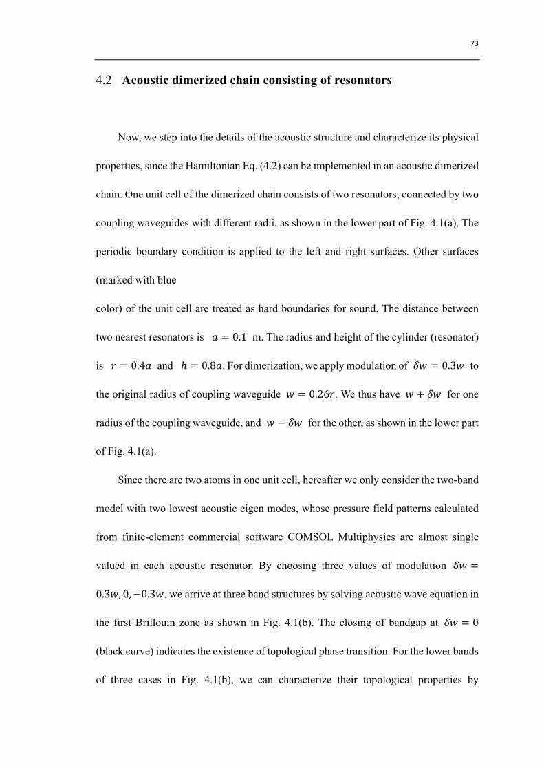
4.2 Acoustic dimerized chain consisting of resonators

Now, we step into the details of the acoustic structure and characterize its physical

properties, since the Hamiltonian Eq. (4.2) can be implemented in an acoustic dimerized

chain. One unit cell of the dimerized chain consists of two resonators, connected by two

coupling waveguides with different radii, as shown in the lower part of Fig. 4.1(a). The

periodic boundary condition is applied to the left and right surfaces. Other surfaces

(marked with blue

color) of the unit cell are treated as hard boundaries for sound. The distance between

two nearest resonators is 𝑎 = 0.1 m. The radius and height of the cylinder (resonator)

is 𝑟 = 0.4𝑎 and ℎ = 0.8𝑎. For dimerization, we apply modulation of 𝛿𝑤 = 0.3𝑤 to

the original radius of coupling waveguide 𝑤 = 0.26𝑟. We thus have 𝑤 + 𝛿𝑤 for one

radius of the coupling waveguide, and 𝑤 − 𝛿𝑤 for the other, as shown in the lower part

of Fig. 4.1(a).

Since there are two atoms in one unit cell, hereafter we only consider the two-band

model with two lowest acoustic eigen modes, whose pressure field patterns calculated

from finite-element commercial software COMSOL Multiphysics are almost single

valued in each acoustic resonator. By choosing three values of modulation 𝛿𝑤 =

0.3𝑤, 0, −0.3𝑤, we arrive at three band structures by solving acoustic wave equation in

the first Brillouin zone as shown in Fig. 4.1(b). The closing of bandgap at 𝛿𝑤 = 0

(black curve) indicates the existence of topological phase transition. For the lower bands

of three cases in Fig. 4.1(b), we can characterize their topological properties by

74

calculating the topological invariant – Zak phase [5, 74, 76, 77] 𝜑¤�) =

𝑖 𝑢/,) 𝛻) 𝑢/,) 𝑑𝑘¥/"�s¥/"� . The results are −𝜋/2, 0 and 𝜋/2 for 𝛿𝑤 > 0, 𝛿𝑤 = 0

and 𝛿𝑤 < 0, respectively. Note that the Zak phase of each dimerization is a gauge

dependent value, but the difference between the Zak phases of two dimerized

configurations with 𝛿𝑤 > 0 and 𝛿𝑤 < 0, which is ∆𝜑¤�) = 𝜑¤�)" − 𝜑¤�)T = 𝜋 in

our acoustic model, is topologically defined. Because the topological property of a

bandgap is determined by the summation of Zak phases of all bands below the gap, the

two dimerizations in Fig. 4.1(b) (red and blue curves) are topologically distinct to each

other.

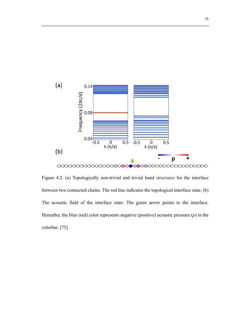
The above topologically nontrivial phases in acoustic resonators ensure the

existence of interface states between two configurations of dimerized lattices with

different Zak phases. Hereafter we cut and connect the two chains through their mirror

centers for physical reasons [78]. The interface dispersions demonstrated in Fig. 4.2(a)

are the results from numerical simulation. For the left panel, we apply 𝛿𝑤 = 0.3𝑤 and

𝛿𝑤 = −0.3𝑤 on two sides of an interface. For the right panel, 𝛿𝑤 = 0.3𝑤 and 𝛿𝑤 =

0.1𝑤 are applied. There is an interface state, predicated, locating inside the bandgap in

the left panel of Fig. 4.2(a), as highlighted by the red line. The acoustic pressure field

pattern of the interface state is shown in Fig. 4.2(b). The green arrow points to the

interface between two topologically distinct structures. We can clearly see that the

amplitude of the acoustic wave decays rapidly into the bulk on both sides of the interface.

75

Figure 4.2. (a) Topologically non-trivial and trivial band structures for the interface

between two connected chains. The red line indicates the topological interface state. (b)

The acoustic field of the interface state. The green arrow points to the interface.

Hereafter, the blue (red) color represents negative (positive) acoustic pressure (p) in the

colorbar. [75]

76

4.3 Dirac nodes in a dimerized square lattice

Utilizing these 1D dimerized chains shown in last section as building blocks, we

can construct 2D Dirac nodes by stacking these 1D dimerized chains in a staggered way.

In the following, we first design the theoretical Hamiltonian for predicting the existence

of 2D Dirac nodes and later 3D Weyl nodes for simplicity. Then we construct the

acoustic structure through following the parameters of the Hamiltonian.

We find that the 2D Dirac nodes can be constructed by the Bloch Hamiltonian of a

2D dimerized acoustic lattice shown below:

𝐻" 𝑘 = [2𝑡J𝑐𝑜𝑠 𝑘J𝑎 + 2𝑡K𝑐𝑜𝑠 𝑘K𝑎 ]𝜎J − 2𝛿𝑡J𝑠𝑖𝑛(𝑘J𝑎)𝜎K,

(4.3)

where 𝑡J (𝑡K) is the hopping strength along x (y) direction, and 𝛿𝑡J is the modulation

of the hopping strength along x direction. Following the above tight-binding model, we

set the unit cell of the acoustic lattice as shown in Fig. 4.3(a). The right inset is the

schematic of 2D lattice whose unit cell is enclosed by green dashed lines. Through

tuning the coupling strength, we find that there are two linear degenerate points in the

first Brillouin zone if 𝑡J < 𝑡K , no degenerate points (trivial band gap) if 𝑡J > 𝑡K ,

and quadratic degenerate points [79] in the corners of 2D Brillouin zone if 𝑡J = 𝑡K .

Here we choose 𝑡J = −1, 𝑡K = −2 and 𝛿𝑡J = −0.5. The band structure in the 2D

momentum space (𝑘J, 𝑘K) , as shown in Fig. 4.3(b), can be calculated from the

Hamiltonian Eq. (4.3), as shown in Fig. 4.3(c). There are two isolated degenerate points

located at (0, ± 2 3) in units of 𝜋 𝑎 in the first 2D Brillouin zone, enclosed by blue

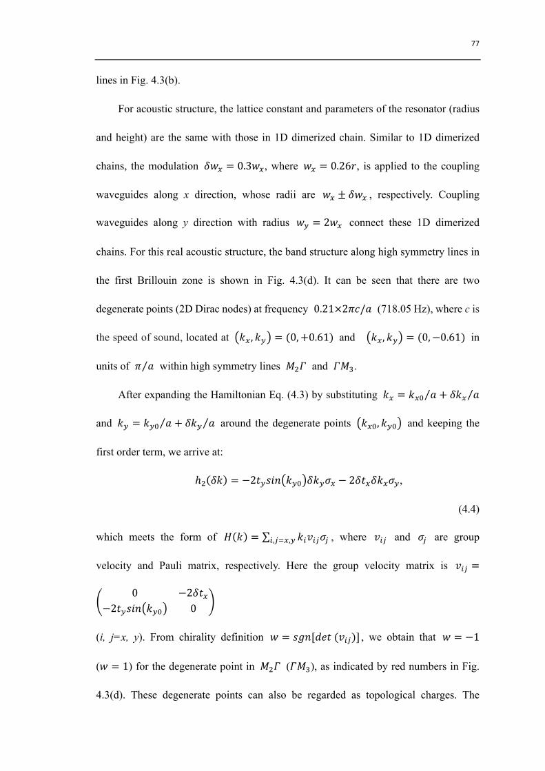
77

lines in Fig. 4.3(b).

For acoustic structure, the lattice constant and parameters of the resonator (radius

and height) are the same with those in 1D dimerized chain. Similar to 1D dimerized

chains, the modulation 𝛿𝑤J = 0.3𝑤J, where 𝑤J = 0.26𝑟, is applied to the coupling

waveguides along x direction, whose radii are 𝑤J ± 𝛿𝑤J , respectively. Coupling

waveguides along y direction with radius 𝑤K = 2𝑤J connect these 1D dimerized

chains. For this real acoustic structure, the band structure along high symmetry lines in

the first Brillouin zone is shown in Fig. 4.3(d). It can be seen that there are two

degenerate points (2D Dirac nodes) at frequency 0.21×2𝜋𝑐/𝑎 (718.05 Hz), where c is

the speed of sound, located at 𝑘J, 𝑘K = (0,+0.61) and 𝑘J, 𝑘K = (0,−0.61) in

units of 𝜋 𝑎 within high symmetry lines 𝑀"𝛤 and 𝛤𝑀m.

After expanding the Hamiltonian Eq. (4.3) by substituting 𝑘J = 𝑘JM 𝑎 + 𝛿𝑘J 𝑎

and 𝑘K = 𝑘KM 𝑎 + 𝛿𝑘K 𝑎 around the degenerate points 𝑘JM, 𝑘KM and keeping the

first order term, we arrive at:

ℎ" 𝛿𝑘 = −2𝑡K𝑠𝑖𝑛 𝑘KM 𝛿𝑘K𝜎J − 2𝛿𝑡J𝛿𝑘J𝜎K,

(4.4)

which meets the form of 𝐻 𝑘 = 𝑘(𝑣(G𝜎G(,GIJ,K , where 𝑣(G and 𝜎G are group

velocity and Pauli matrix, respectively. Here the group velocity matrix is 𝑣(G =

0 −2𝛿𝑡J−2𝑡K𝑠𝑖𝑛 𝑘KM 0

(i, j=x, y). From chirality definition 𝑤 = 𝑠𝑔𝑛[𝑑𝑒𝑡(𝑣(G)] , we obtain that 𝑤 = −1

(𝑤 = 1) for the degenerate point in 𝑀"𝛤 (𝛤𝑀m), as indicated by red numbers in Fig.

4.3(d). These degenerate points can also be regarded as topological charges. The

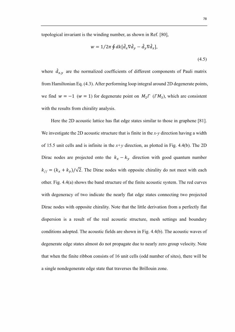
78

topological invariant is the winding number, as shown in Ref. [80],

𝑤 = 1 2𝜋 𝑑𝑘[𝑑J∇𝑑K − 𝑑K∇𝑑J],

(4.5)

where 𝑑J,K are the normalized coefficients of different components of Pauli matrix

from Hamiltonian Eq. (4.3). After performing loop integral around 2D degenerate points,

we find 𝑤 = −1 (𝑤 = 1) for degenerate point on 𝑀"𝛤 (𝛤𝑀m), which are consistent

with the results from chirality analysis.

Here the 2D acoustic lattice has flat edge states similar to those in graphene [81].

We investigate the 2D acoustic structure that is finite in the x-y direction having a width

of 15.5 unit cells and is infinite in the x+y direction, as plotted in Fig. 4.4(b). The 2D

Dirac nodes are projected onto the 𝑘J − 𝑘K direction with good quantum number

𝑘// = (𝑘J + 𝑘K)/ 2. The Dirac nodes with opposite chirality do not meet with each

other. Fig. 4.4(a) shows the band structure of the finite acoustic system. The red curves

with degeneracy of two indicate the nearly flat edge states connecting two projected

Dirac nodes with opposite chirality. Note that the little derivation from a perfectly flat

dispersion is a result of the real acoustic structure, mesh settings and boundary

conditions adopted. The acoustic fields are shown in Fig. 4.4(b). The acoustic waves of

degenerate edge states almost do not propagate due to nearly zero group velocity. Note

that when the finite ribbon consists of 16 unit cells (odd number of sites), there will be

a single nondegenerate edge state that traverses the Brillouin zone.

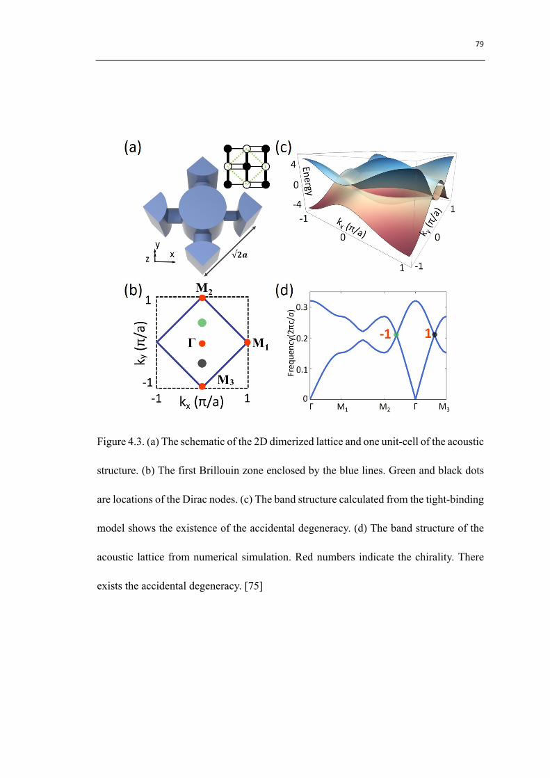
79

Figure 4.3. (a) The schematic of the 2D dimerized lattice and one unit-cell of the acoustic

structure. (b) The first Brillouin zone enclosed by the blue lines. Green and black dots

are locations of the Dirac nodes. (c) The band structure calculated from the tight-binding

model shows the existence of the accidental degeneracy. (d) The band structure of the

acoustic lattice from numerical simulation. Red numbers indicate the chirality. There

exists the accidental degeneracy. [75]

80

Figure 4.4. (a) The band structure for a finite acoustic lattice. The red curves indicate

the flat edge states, which means the nearly zero group velocity. (b) The acoustic fields

of the edge states. Acoustic waves are localized at the edges of the sample. [75]

81

Chapter 5

Acoustic type-II Weyl nodes from stacking dimerized chains

Following the development of Weyl physics in condensed matter physics [15-17]

and photonics [18, 23], in acoustics, 3D Weyl nodes were first proposed theoretically by

applying on-site unequal coupling as shown in Fig. 5.1(a) or chiral coupling on a

graphite structure [82] as shown in Fig. 5.1(c). Fig. 5.1(b, d) present the distributions of

the Weyl nodes corresponding to the two methods and their dispersion as a function of

kz at the Brillouin zone corners. The Weyl nodes associated with the structure shown in

Fig. 5.1(a) [Fig. 5.1(b)] is type-II (type-I) Weyl nodes. However, by that time, the

classification of type-I and type-II Weyl fermions has not been officially addressed in

condensed matter physics and photonics. Consequently, the proposal based on the

graphite structure did not distinguish type-I and type-II Weyl Hamiltonians and only

acoustic topological surface states for type-I Weyl nodes was further studied. In this

Chapter, on a platform of stacked dimerized chains of acoustic resonators, we construct

acoustic type-II Weyl nodes following the explicit type-II Weyl Hamiltonian [21].

Unique features of this acoustic type-II Weyl system include the distinct finite density

of states and transport properties of topological surface states. In a certain momentum

space direction, the bands of the surface states have the same sign of velocity, which is

determined by the tilting direction of type-II Weyl nodes rather than their chirality

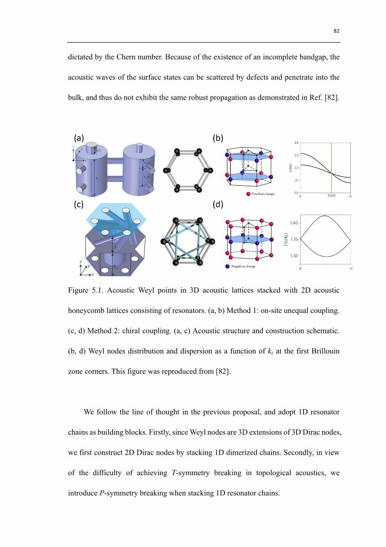
82

dictated by the Chern number. Because of the existence of an incomplete bandgap, the

acoustic waves of the surface states can be scattered by defects and penetrate into the

bulk, and thus do not exhibit the same robust propagation as demonstrated in Ref. [82].

Figure 5.1. Acoustic Weyl points in 3D acoustic lattices stacked with 2D acoustic

honeycomb lattices consisting of resonators. (a, b) Method 1: on-site unequal coupling.

(c, d) Method 2: chiral coupling. (a, c) Acoustic structure and construction schematic.

(b, d) Weyl nodes distribution and dispersion as a function of kz at the first Brillouin

zone corners. This figure was reproduced from [82].

We follow the line of thought in the previous proposal, and adopt 1D resonator

chains as building blocks. Firstly, since Weyl nodes are 3D extensions of 3D Dirac nodes,

we first construct 2D Dirac nodes by stacking 1D dimerized chains. Secondly, in view

of the difficulty of achieving T-symmetry breaking in topological acoustics, we

introduce P-symmetry breaking when stacking 1D resonator chains.

83

5.1 Type-II Weyl nodes in a dimerized cubic lattice

Finally, by stacking the 2D dimerized lattice as in section 3.2 along the z direction

with periodicity a and tuning the coupling strength, we can construct a Bloch

Hamiltonian for the 3D dimerized lattice:

𝐻m 𝑘 = 𝑑M𝐼 + 𝑑J𝜎J + 𝑑K𝜎K + 𝑑L𝜎L,

(5.1)

where 𝑑J = 2𝑡J𝑐𝑜𝑠 𝑘J𝑎 + 2𝑡K𝑐𝑜𝑠 𝑘K𝑎 , 𝑑K = −2𝛿𝑡J𝑠𝑖𝑛(𝑘J𝑎) , 𝑑L =

𝑡LT𝑐𝑜𝑠 𝑘L𝑎 − 𝑡L"𝑐𝑜𝑠 𝑘L𝑎 , 𝑑M = 𝑡LT𝑐𝑜𝑠 𝑘L𝑎 + 𝑡L"𝑐𝑜𝑠 𝑘L𝑎 and 𝐼 is the 2×2

identity matrix. The parameter 𝑡J (𝑡K,𝑡L) is the hopping strength along x (y, z) direction.

Note that the first term in Eq. (5.1) plays the role of tilting the cone-like spectrum. With

a strongly tilted cone spectrum, this Hamiltonian satisfies the condition of recently

proposed type-II Weyl Hamiltonian [21] 𝐻 𝑘 = 𝑘(𝑣(G𝜎G(IJ,K,LGIM,J,K,L

.

Hereafter we choose 𝑡J = −1 , 𝑡K = −2 , 𝑡LT = −1 , 𝑡L" = −2 and 𝛿𝑡J =

−0.5, as schematically shown in Fig. 5.2(a). The Hamiltonian breaks P-symmetry and

respects T-symmetry. We calculate the band structure as shown in Fig. 5.2(b) with 𝑘L =

0.5 in 𝑘J − 𝑘K Brillouin zone plane. Four linear degenerate points locate at

(0, ± 2 3 ,±1 2) in units of 𝜋 𝑎 in the 3D first Brillouin zone. Typically, we plot in

Fig. 5.2(c) the cone spectrum in the vicinity of the degenerate point (0, 2 3 , 1 2) in

𝑘J − 𝑘K Brillouin zone plane. It can be seen that the cone spectrum indeed has been

strongly tilted. Since the group velocities along z direction near the degenerate point are

2𝑡LT𝑠𝑖𝑛 𝑘LM and 2𝑡L"𝑠𝑖𝑛 𝑘LM where 𝑘LM is the location of degenerate point, the

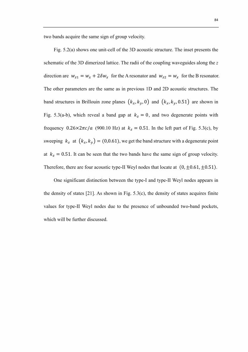
84

two bands acquire the same sign of group velocity.

Fig. 5.2(a) shows one unit-cell of the 3D acoustic structure. The inset presents the

schematic of the 3D dimerized lattice. The radii of the coupling waveguides along the z

direction are 𝑤LT = 𝑤J + 2𝛿𝑤J for the A resonator and 𝑤L" = 𝑤J for the B resonator.

The other parameters are the same as in previous 1D and 2D acoustic structures. The

band structures in Brillouin zone planes 𝑘J, 𝑘K, 0 and 𝑘J, 𝑘K, 0.51 are shown in

Fig. 5.3(a-b), which reveal a band gap at 𝑘L = 0, and two degenerate points with

frequency 0.26×2𝜋𝑐/𝑎 (900.10 Hz) at 𝑘L = 0.51. In the left part of Fig. 5.3(c), by

sweeping 𝑘L at 𝑘J, 𝑘K = (0,0.61), we get the band structure with a degenerate point

at 𝑘L = 0.51. It can be seen that the two bands have the same sign of group velocity.

Therefore, there are four acoustic type-II Weyl nodes that locate at 0,±0.61, ±0.51 .

One significant distinction between the type-I and type-II Weyl nodes appears in

the density of states [21]. As shown in Fig. 5.3(c), the density of states acquires finite

values for type-II Weyl nodes due to the presence of unbounded two-band pockets,

which will be further discussed.

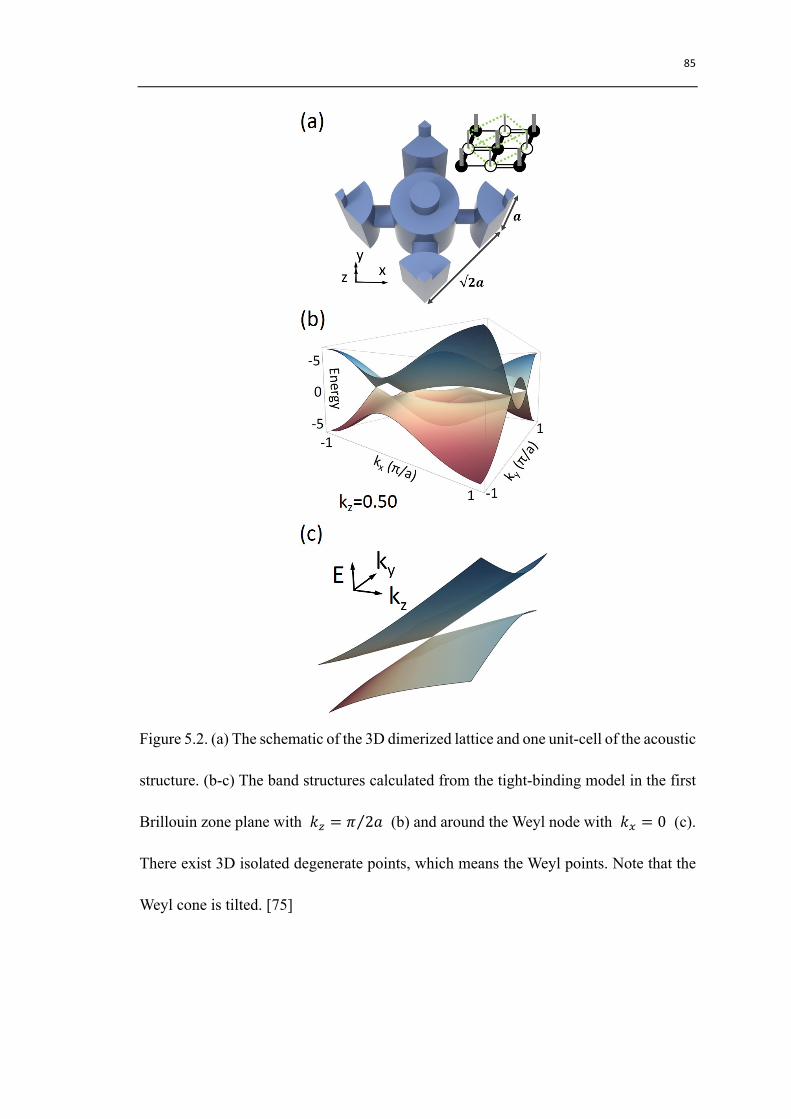
85

Figure 5.2. (a) The schematic of the 3D dimerized lattice and one unit-cell of the acoustic

structure. (b-c) The band structures calculated from the tight-binding model in the first

Brillouin zone plane with 𝑘L = 𝜋 2𝑎 (b) and around the Weyl node with 𝑘J = 0 (c).

There exist 3D isolated degenerate points, which means the Weyl points. Note that the

Weyl cone is tilted. [75]

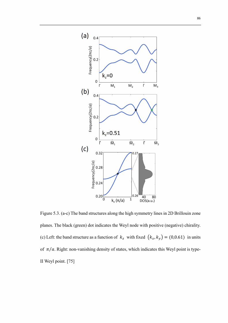
86

Figure 5.3. (a-c) The band structures along the high symmetry lines in 2D Brillouin zone

planes. The black (green) dot indicates the Weyl node with positive (negative) chirality.

(c) Left: the band structure as a function of 𝑘L with fixed 𝑘J, 𝑘K = (0,0.61) in units

of 𝜋 𝑎. Right: non-vanishing density of states, which indicates this Weyl point is type-

II Weyl point. [75]

87

5.2 Chirality of the Weyl nodes

Because the Chern number is not changed by the first term [21] of the Hamiltonian

Eq. (5.1), we expand the Pauli-matrix components around the Weyl node by substituting

𝑘J = 𝑘JM 𝑎 + 𝛿𝑘J 𝑎 , 𝑘K = 𝑘KM 𝑎 + 𝛿𝑘K 𝑎 and 𝑘L = 𝑘LM 𝑎 + 𝛿𝑘L 𝑎 around the

Weyl nodes 𝑘JM, 𝑘KM, 𝑘LM and keeping the first-order terms and Pauli-matrix terms,

we have:

ℎm 𝛿𝑘 = −2𝑡K𝑠𝑖𝑛 𝑘KM 𝛿𝑘K𝜎J − 2𝛿𝑡J𝛿𝑘J𝜎K − (𝑡LT𝑠𝑖𝑛 𝑘LM 𝛿𝑘L

− 𝑡L"𝑠𝑖𝑛 𝑘LM 𝛿𝑘L)𝜎L

(5.2)

which meets the expression of 𝐻 𝑘 = 𝑘(𝑣(G𝜎G(,GIJ,K , where 𝑣(G (i, j=x, y, z) and 𝜎G

are group velocity and Pauli matrix, respectively. In the 3D momentum space, the Weyl

nodes are topological monopoles of quantized Berry flux characterized by the chirality

𝑐 = 𝑠𝑔𝑛[𝑑𝑒𝑡(𝑣(G)] , or the topological invariant—Chern number. Here the group

velocity matrix from Eqn. (3.5) is:

𝑣(G =0 −2𝛿𝑡J 0

−2𝑡K𝑠𝑖𝑛 𝑘KM 0 00 0 −𝑡LT𝑠𝑖𝑛 𝑘LM + 𝑡L"𝑠𝑖𝑛 𝑘LM

.

(5.3)

Therefore the chirality is 𝑐 = 1 (𝑐 = −1) for 0, 2 3 , 1 2 and 0,−2 3 ,−1 2

[ 0, 2 3 , −1 2 and 0,−2 3 , 1 2 ], which are indicated by black “+” (green “-”) in

the momentum plane 0, 𝑘K, 𝑘L as shown in Fig. 5.4(a). From above equations, an

analytical expression for Berry curvature around the Weyl point 0, 2 3 , −1 2 is

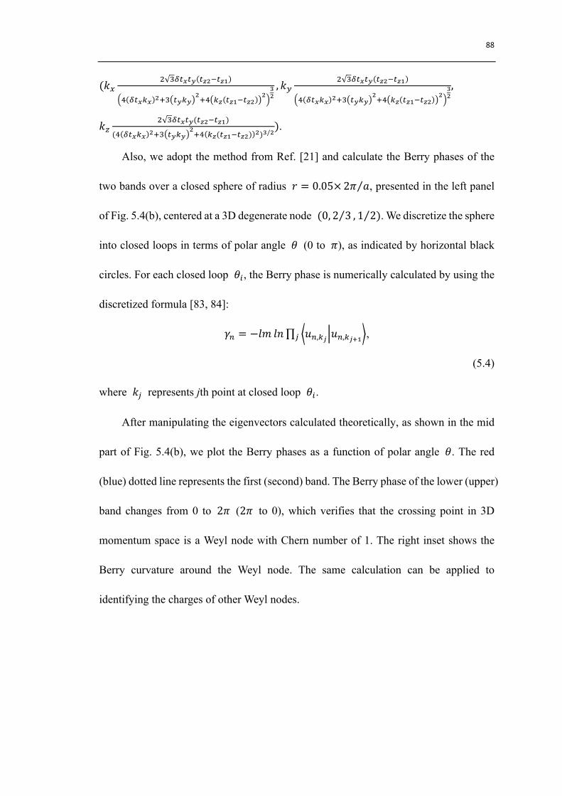
88

(𝑘J" mªv«v¬ v­rsv­q

� ªv«)« r�m v¬)¬r�� )­ v­qsv­r

rWr, 𝑘K

" mªv«v¬ v­rsv­q

� ªv«)« r�m v¬)¬r�� )­ v­qsv­r

rWr,

𝑘L" mªv«v¬(v­rsv­q)

(� ªv«)« r�m v¬)¬r�� )­(v­qsv­r) r)W/r

).

Also, we adopt the method from Ref. [21] and calculate the Berry phases of the

two bands over a closed sphere of radius 𝑟 = 0.05×2𝜋 𝑎, presented in the left panel

of Fig. 5.4(b), centered at a 3D degenerate node (0, 2 3 , 1 2). We discretize the sphere

into closed loops in terms of polar angle 𝜃 (0 to 𝜋), as indicated by horizontal black

circles. For each closed loop 𝜃(, the Berry phase is numerically calculated by using the

discretized formula [83, 84]:

𝛾/ = −𝑙𝑚 𝑙𝑛 𝑢/,)° 𝑢/,)°±qG ,

(5.4)

where 𝑘G represents jth point at closed loop 𝜃(.

After manipulating the eigenvectors calculated theoretically, as shown in the mid

part of Fig. 5.4(b), we plot the Berry phases as a function of polar angle 𝜃. The red

(blue) dotted line represents the first (second) band. The Berry phase of the lower (upper)

band changes from 0 to 2𝜋 (2𝜋 to 0), which verifies that the crossing point in 3D

momentum space is a Weyl node with Chern number of 1. The right inset shows the

Berry curvature around the Weyl node. The same calculation can be applied to

identifying the charges of other Weyl nodes.

89

Figure 5.4. (a) The distribution of type-II Weyl nodes in 3D first Brillouin zone. Black

“+” (green “-”) indicates the positive (negative) chirality. (b) Left panel: A sphere in

momentum space enclosing one Weyl point. The radius of the sphere is 0.05×2π/a.

Right panel: Berry phase and Berry curvature around the Weyl point (0, 2 3 , 1 2). [75]

90

5.3 Fermi-arc-like surface state

The nonzero Chern numbers imply the existence of topological surface states. We

investigate the 3D acoustic structure that is finite in the x-y direction and infinite in the

x+y and z directions. In this case, the Weyl nodes are projected along the 𝑘J − 𝑘K

direction, indicated by black and green dotted points in Fig. 5.5(d), with good quantum

numbers 𝑘// = (𝑘J + 𝑘K)/ 2 and 𝑘L . Fig. 5.5(a-b) show the projected band

structures with fixed 𝑘// = 1/ 2 [Fig. 5.5(a)] and 𝑘// = 0 [Fig. 5.5(b)] in units of

𝜋 𝑎, as indicated by “Cut 1” and “Cut 2” in Fig. 5.5(d). In Fig. 5.5(a), two surface states

(red and green curves), corresponding to the two opposite surfaces, are located in an

incomplete bandgap and both acquireing positive group velocity. In Fig. 5.5(b), no

surface states show up. As presented in Fig. 5.5(c), the upper (lower) acoustic field

corresponds to the surface state of green (red) curve in Fig. 5.5(a). We also plot the

sound intensity 𝑰 = 𝑝𝒗 (𝑝 is sound pressure and 𝒗 is the velocity) as grey arrows,

whose length represents the amplitude of sound intensity. Both the two surface states

propagate along the z direction, which is consistent with the positive group velocity in

Fig. 5.5(a).

To demonstrate the acoustic open “Fermi arcs,” we trace out the trajectories of

surface states at frequency 0.26×2𝜋𝑐/𝑎 (900.1 Hz) in the 2D Brillouin zone (𝑘//, 𝑘L),

as indicated by red dotted points in Fig. 5.5(d). Here we consider a semi-infinite system

and thus only the surface states localized at one surface [red curve in Fig. 5.5(a)] are

included. These trajectories indeed connect two pairs of type-II Weyl nodes, as an analog

91

of open Fermi arcs in type-II Weyl semimetals [21].

Figure 5.5. (a-b) The band structures with 𝑘// = 1/ 2 (a) and 𝑘// = 0 (b). The red

and green curves indicate the surface states. (c) The acoustic fields of the surface states

in panel (a). The acoustic fields are localized at the edges. The grey arrows represent the

sound intensity. (d) Red dotted points indicate the trajectories of the “Fermi Arc” in the

2D surface Brillouin zone. Black dots (green dots) indicate Weyl points with positive

(negative) chirality. [75]

92

5.4 Distinct features

Firstly, one significant distinction between the type-I and type-II Weyl nodes

appears in the density of states. The equation of density of states is expressed as 𝑔 ω =

µ("¥)W

𝛿(𝜔 − 𝜔(𝑘))𝑑m𝑘, where V is the volume of contributed momentum box in the

vicinity of the Weyl node. For type-I Weyl nodes, the density of states vanishes at the

frequency of Weyl nodes. However, the density of states acquires finite values for type-

II Weyl nodes due to the presence of unbounded two-band pockets. We retrieve the

parameters from fitting the data of bands with the Eq. (5.1) and plot the density of states

that arises due to the type-II Weyl node in the right part of Fig. 5.3(c). The contribution

of the other iso-frequency surface to the density of states is not included. The peak

indicates the location of the type-II Weyl node.

Secondly, as presented in Fig. 5.5(a), the positive group velocity of the surface

states is determined by the strong tilted cone spectrum of type-II Weyl nodes. For 𝑘¶ >

0 with fixed 𝑘// = 1/ 2, the two surface states localized at the opposite surfaces of

the system both acquire group velocities of the same positive sign. In contrast, in the

previously demonstrated topological surface states [82] of acoustic type-I system, their

propagation direction is surface-dependent: if the surface states on one surface

propagate in one direction, those on the opposite surface should propagate in the

opposite direction. This distinction is schematically illustrated in Fig. 5.6(a).

Thirdly, another distinction is that the surface states of type-II Weyl nodes stay in

an incomplete bandgap. By putting sound sources with frequency 0.26×2𝜋𝑐/𝑎 (900.1

93

Hz) at the surface of the acoustic type-II Weyl system, we can study the propagation

features of the surface states. As shown in Fig. 5.6(b), we consider a structure that is

finite in the x-y direction. Under the condition of single-frequency excitation, the surface

states as well as the bulk states can both be excited by the sound source, as a

consequence of the incomplete bandgap associated with type-II Weyl node. At the two

bottom corners, the surface states will get scattered into the bulk because of the existence

of backscattering modes. Therefore, they do not have the same robustness (scattering-

immunity against defects) as demonstrated in Ref. [82], but the existence of open “Fermi

arcs” connecting Weyl nodes in the momentum space is robust.

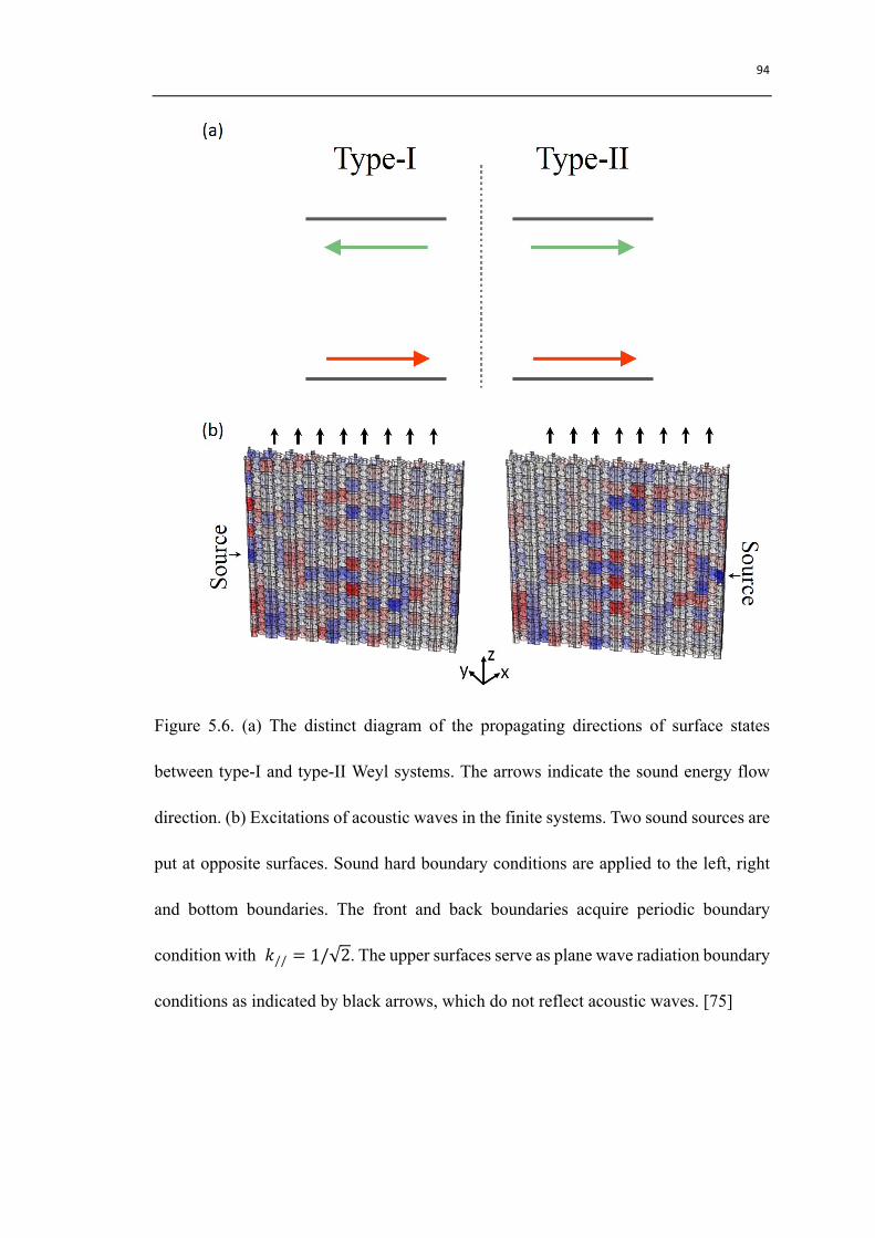
94

Figure 5.6. (a) The distinct diagram of the propagating directions of surface states

between type-I and type-II Weyl systems. The arrows indicate the sound energy flow

direction. (b) Excitations of acoustic waves in the finite systems. Two sound sources are

put at opposite surfaces. Sound hard boundary conditions are applied to the left, right

and bottom boundaries. The front and back boundaries acquire periodic boundary

condition with 𝑘// = 1/ 2. The upper surfaces serve as plane wave radiation boundary

conditions as indicated by black arrows, which do not reflect acoustic waves. [75]

95

5.5 Conclusion

The above results demonstrate the feasibility of constructing acoustic type-II Weyl

nodes by stacking 1D dimerized chains of acoustic resonators. The unique features of

acoustic type-II Weyl system, such as the finite density of states and transport properties

of surface states, are demonstrated. The Fermi-arc-like surface states can be traced out

as an analog of Fermi arcs in recently demonstrated type-II Weyl semimetals. The

stacking method shown in this work provides an approach of constructing topological

phases at different dimensions with the same building blocks, and may be extended to

other systems including cold atoms [76, 85] and photonics [6, 27].

96

Summary and future work

In this thesis, I have studied two types of acoustic crystals in two dimension and

three dimension, respectively. I extend the quantum Hall effect into acoustics and

explore the distinct features of the type-II Weyl nodes in a 3D acoustic lattice.

Firstly, the time-reversal symmetry can be broken in an acoustic crystal by

incorporating circulating air flow. We can see that the unconventional acoustic crystal

exhibits a topological band gap from opening the Dirac cone. The band below the gap

acquires a non-zero Chern number, which ensures the existence of the topologically

protected one-way acoustic edge state.

Secondly, we construct the acoustic version of type-II Weyl Hamiltonian by

stacking one-dimensional dimerized chains of acoustic resonators. This acoustic type-II

Weyl system exhibits distinct features in finite density of states and unique transport

properties of Fermi-arc-like surface states. In a certain momentum space direction, the

velocity of these surface states are determined by the tilting direction of the type-II Weyl

nodes, rather than the chirality dictated by the Chern number.

It has been about two years since the first topological acoustic paper was published.

The field named “topological acoustics [44, 53, 75, 86-89]” or even bigger category

“topological bosonics [27, 43, 90, 91]” has drawn a lot of attention in both theoretical

proposals and experimental realizations. Most importantly, there is still much work that

remains to be explored.

97

In the next, I suggest some of the potential projects for future work.

Firstly, we can introduce strain engineering into a two-dimensional acoustic

structure in order to form a uniform effective magnetic field for airborne acoustic wave

propagation. Landau levels in the energy spectrum can be formed near the Dirac cone

region. We have built an experimental setup to verify the existence of acoustic Landau

levels with an acoustic measurement.

Secondly, inspired by the recent progress in higher-dimensional topological phases

in condensed matter physics and photonics, I try to build a two-dimensional square

lattice consisting of compressibility-modulated acoustic resonators to investigate the

four-dimensional quantum Hall effect. By modulating the resonators in one dimension,

we can realize one-dimensional Harper model, which the on-site potential is modulated.

Through adding the modulation along the second direction, we can implement 4D

quantum Hall effect for acoustic waves, which is associated with nonzero second Chern

numbers.

Thirdly, we can experimentally demonstrate valley-polarized kink states in valley

photonic crystals, designed from a four-band model. When the valley pseudospin is

conserved, we show that the kink states exhibit perfect out-coupling efficiency into

directional beams, through the intersection between the internal domain wall and the

external edge separating the valley photonic crystals from ambient space. Interestingly,

the valley Hall effect of four-band model can be mapped into phononic metamaterials

for elastic waves.

98

Appendix A

Plane wave expansion method

In a triangular phononic crystal with air flow, master equation is given as:

Tx𝛻 ∙ 𝜌𝛻𝜙 − 𝜕v + 𝑣M ∙ 𝛻

Tzr

𝜕v + 𝑣M ∙ 𝛻 𝜙 = 0,

(A1)

where 𝜌 and 𝑐 are the spatially-dependent density and sound velocity of air,

respectively. The velocity field has two components: 𝑣* = 0 and 𝑣o = − p*qr

*rrs*qr𝑟 +

p*qr*rr

*rrs*qrT*, where 𝑟 is measured in localized coordinates centered at each hexagonal unit

cell, 𝜃 is the azimuthal angle in each unit cell.

To find solutions of Eq. (A1), we neglect terms of second order 𝑣M 𝑐 " ≪ 1, and

keep the first order, we have

zr

x𝛻 ∙ 𝜌𝛻𝜙 − 2𝜕v𝑣M ∙ 𝛻𝜙 = 𝜕v"𝜙,

(A2)

Then we perform the Plane Wave Expansion Method by expanding the velocity

potential 𝜙 and spatial parameters in terms of plane waves,

𝜙 𝑟, 𝑞 = 𝜙¸𝑒((¹�¸)∙*¸ , zr

x𝑟 = 𝜌′¸𝑒(¸∙*¸ , 𝜌 𝑟 = 𝜌¸𝑒(¸∙*¸ ,

𝑣J 𝑟 = 𝑣J¸𝑒(¸∙*¸ , 𝑣K 𝑟 = 𝑣K¸𝑒(¸∙*¸ .

(A3)

By substituting equation (A3) into (A2), we obtain the linear equation for the Fourier

component of the velocity potential,

{−𝜌¼¸"s¸¼𝜌¼¸¾s¸ 𝑞J + 𝐺J 𝑞J + 𝐺¼J + 𝑞K + 𝐺K 𝑞K + 𝐺¼K¸"¸¼

99

−2𝜔 𝑣J¸"s¸ 𝑞J + 𝐺J + 𝑣K¸"s¸ 𝑞K + 𝐺K }𝜙¸ = −𝜔"𝜙¸ .

(A4)

Numerically we can obtain the eigen frequencies and eigen states of our phononic

crystal by solving above matrix.

We now analysis the Dirac cones in the vicinity of 𝐾 point. In the situation we

truncate the plane wave basis to the three nearest 𝛤 points. And the three equal length

reciprocal lattice vectors 𝑲+ 𝑮𝒊 each rotated 2𝜋/3 with respect to one another. 𝑲

is a vector pointing from 𝛤 point to 𝐾 point and 𝑖 = 0,1,2 indexes the three

reciprocal lattice vectors. Then in the vicinity of the 𝐾 point 𝑞J = |𝑲| + 𝛿𝑘J and

𝑞K = 𝛿𝑘K, where the length of 𝑲 equals to 4𝜋/(3𝑎), a 3×3 Hermitian equation can

be obtained. Performing the transformation 𝑈 = 1 3 [1,1,1; 1, 𝜂", 𝜂; 1, 𝜂, 𝜂"], where

𝜂 = 𝑒𝑥𝑝(𝑖2𝜋/3) , we can get effective Hamiltonian of the two Dirac bands by

eliminating the singlet,

𝑑(𝛿𝒌, 𝒗𝑮, 𝒗′𝑮) 𝑣Æ 𝛿𝑘J − 𝑖𝛿𝑘K + 𝜅Ç − 𝑖𝜅È𝑣Æ 𝛿𝑘J + 𝑖𝛿𝑘K + 𝜅Ç + 𝑖𝜅È 𝑑(𝛿𝒌, 𝒗𝑮, 𝒗′𝑮)

𝜙 = 𝛺𝜙,

(A5)

where

𝑑 𝛿𝑘, 𝒗𝑮, 𝒗¼𝑮 = 𝜔[ 𝑣J¸M − 𝑣J¸T 𝛿𝑘J + 𝑣K¸M − 𝑣K¸T 𝛿𝑘K],

𝑣Æ = 𝐾𝜌¼¸((𝜌¸M − 𝜌¸T),

𝜅Ç =��"[𝑣J¸T − 𝑣J¸M],

𝜅È =��"[𝑣K¸T − 𝑣K¸M],

𝛺 = 𝜔" + �r

"𝜌¼¸((2𝜌¸M + 𝜌¸T).

(A6)

100

And i=0, 1, 2 indicates the summation of three components.

We can rewritten equation (A5) as

𝐻 𝑘 = 𝑑 𝑘 𝐼 + 𝑣Æ𝛿𝑘J + 𝜅Ç 𝜎J + 𝑣Æ𝛿𝑘K + 𝜅È 𝜎K.

(A7)

where 𝐼 is 2×2 identity matrix. Under transformation 𝜎( → −𝜎( and 𝑘( → −𝑘(, we

know that 𝑇 𝐻 𝑘 𝑇 ≠ 𝐻 −𝑘 , which indicates that the time-reversal symmetry is

broken.

As we can see that (A7) will be mapped to massless Dirac-like equation if there is

no air flow. And the linear dispersion is,

𝜔 = 𝜔Æ ± 𝑣Æ|𝛿𝒌|.

(A8)

The flow induced the first term 𝑑(𝑘) as shown in Eq. (A7), which is small when the

circulation is less than 𝛤z = 2𝜋×4, can shift the global energy at the Dirac point. The

terms 𝜅Ç and 𝜅È changing the momentum can be simply understood as Doppler effect

[3]. Using the expression for the Dirac point, we find the dispersion relation of the Dirac

bands is now given by

𝜔 = 𝜔′Æ ± |𝑣Æ𝛿𝑘J + 𝜅Ç|" + |𝑣Æ𝛿𝑘K + 𝜅È|"

(A9)

The degeneracy is lifted and the band gap at Dirac point is 𝜿 = |𝜅Ç|" + |𝜅È|"

determined by reciprocal components of flow velocity. Similar method can be applied

to 𝐾′ point.

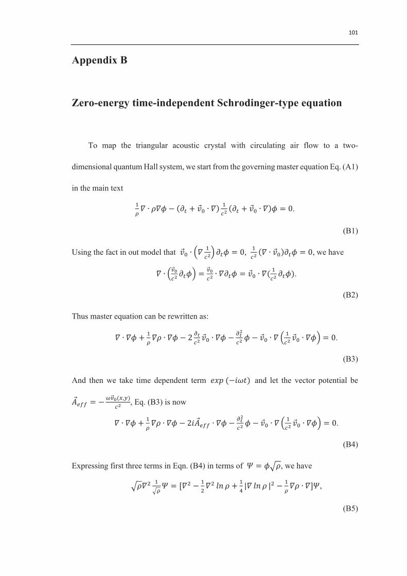
101

Appendix B

Zero-energy time-independent Schrodinger-type equation

To map the triangular acoustic crystal with circulating air flow to a two-

dimensional quantum Hall system, we start from the governing master equation Eq. (A1)

in the main text

Tx𝛻 ∙ 𝜌𝛻𝜙 − 𝜕v + 𝑣M ∙ 𝛻

Tzr

𝜕v + 𝑣M ∙ 𝛻 𝜙 = 0.

(B1)

Using the fact in out model that 𝑣M ∙ 𝛻Tzr

𝜕v𝜙 = 0, Tzr

𝛻 ∙ 𝑣M 𝜕v𝜙 = 0, we have

𝛻 ∙ ÊËzr𝜕v𝜙 = ÊË

zr∙ 𝛻𝜕v𝜙 = 𝑣M ∙ 𝛻(

Tzr𝜕v𝜙).

(B2)

Thus master equation can be rewritten as:

𝛻 ∙ 𝛻𝜙 + Tx𝛻𝜌 ∙ 𝛻𝜙 − 2 �Ì

zr𝑣M ∙ 𝛻𝜙 −

�Ìr

zr𝜙 − 𝑣M ∙ 𝛻

Tzr𝑣M ∙ 𝛻𝜙 = 0.

(B3)

And then we take time dependent term 𝑒𝑥𝑝(−𝑖𝜔𝑡) and let the vector potential be

𝐴~�� = −�ÊË(J,K)zr

, Eq. (B3) is now

𝛻 ∙ 𝛻𝜙 + Tx𝛻𝜌 ∙ 𝛻𝜙 − 2𝑖𝐴~�� ∙ 𝛻𝜙 −

�Ìr

zr𝜙 − 𝑣M ∙ 𝛻

Tzr𝑣M ∙ 𝛻𝜙 = 0.

(B4)

Expressing first three terms in Eqn. (B4) in terms of 𝛹 = 𝜙 𝜌, we have

𝜌𝛻" Tx𝛹 = [𝛻" − T

"𝛻" 𝑙𝑛 𝜌 + T

�|𝛻 𝑙𝑛 𝜌 |" − T

x𝛻𝜌 ∙ 𝛻]𝛹,

(B5)

102

𝜌 Tx𝛻𝜌 ∙ 𝛻 T

x𝛹 = [T

x𝛻𝜌 ∙ 𝛻 − T

"|𝛻 𝑙𝑛 𝜌 |"]𝛹

(B6)

− 𝜌2𝑖𝐴~�� ∙ 𝛻Tx𝛹 = [−2𝑖𝐴~�� ∙ 𝛻 + 𝑖𝐴~�� ∙

Tx𝛻𝜌]𝛹

(B7)

In the main text, we study our acoustic system under the condition of low Mach

number, which means 𝑣M 𝑐 ≤ 0.3 . Therefore by neglecting second order terms

( 𝑣M 𝑐 " ≪ 1) and substituting Eqn. (B5, B6, B7) into Eq. (B4), we finally arrive at the

Schrodinger type equation

𝛻 − 𝑖𝐴~��"+ 𝑉 𝑥, 𝑦 𝛹 = 0,

(B8)

where

𝐴~�� = −�ÊË(J,K)zr

(B9)

𝑉 𝑥, 𝑦 = − T�𝛻 𝑙𝑛 𝜌 " − T

"𝛻" 𝑙𝑛 𝜌 + �r

zr.

(B10)

The Eqn. (B8) is the equation for zero-energy wave functions in periodic vector and

scalar potentials, which can map our model to a similar problem in a quantum Hall

system. We should note that we simplify our formulas by neglecting the second order

perturbation, but the vector potential is also a function of frequency. Therefore the

formulas work well for our acoustic system operating at the low frequency energy bands.

However when we consider the system in much high frequency region, the term |𝐴~��|"

contributing to scalar potential cannot be neglected any more in the above derivation

103

procedures.

104

Bibliography

1. K. von Klitzing, "The quantized Hall effect," Reviews of Modern Physics 58, 519-

531 (1986).

2. D. J. Thouless, M. Kohmoto, M. P. Nightingale, and M. den Nijs, "Quantized Hall

Conductance in a Two-Dimensional Periodic Potential," Physical review letters 49,

405-408 (1982).

3. M. Z. Hasan, and C. L. Kane, "Colloquium: Topological insulators," Reviews of

Modern Physics 82, 3045-3067 (2010).

4. X.-L. Qi, and S.-C. Zhang, "Topological insulators and superconductors," Reviews

of Modern Physics 83, 1057-1110 (2011).

5. J. Zak, "Berry's phase for energy bands in solids," Physical review letters 62, 2747-

2750 (1989).

6. L. Lu, J. D. Joannopoulos, and M. Soljačić, "Topological photonics," Nature

Photonics 8, 821-829 (2014).

7. V. H. Weyl, "Elektron und Gravitation. I.," Z. Phys. 56 (1929).

8. F. D. Haldane, and S. Raghu, "Possible realization of directional optical

105

waveguides in photonic crystals with broken time-reversal symmetry," Physical

review letters 100, 013904 (2008).

9. Z. Wang, Y. Chong, J. D. Joannopoulos, and M. Soljacic, "Observation of

unidirectional backscattering-immune topological electromagnetic states," Nature

461, 772-775 (2009).

10. Z. Wang, Y. D. Chong, J. D. Joannopoulos, and M. Soljacic, "Reflection-free one-

way edge modes in a gyromagnetic photonic crystal," Physical review letters 100,

013905 (2008).

11. M. Hafezi, E. A. Demler, M. D. Lukin, and J. M. Taylor, "Robust optical delay

lines with topological protection," Nature Physics 7, 907-912 (2011).

12. M. Hafezi, S. Mittal, J. Fan, A. Migdall, and J. M. Taylor, "Imaging topological

edge states in silicon photonics," Nature Photonics 7, 1001-1005 (2013).

13. K. Fang, Z. Yu, and S. Fan, "Realizing effective magnetic field for photons by

controlling the phase of dynamic modulation," Nature Photonics 6, 782-787 (2012).

14. M. C. Rechtsman, J. M. Zeuner, Y. Plotnik, Y. Lumer, D. Podolsky, F. Dreisow, S.

Nolte, M. Segev, and A. Szameit, "Photonic Floquet topological insulators," Nature

496, 196-200 (2013).

15. X. Wan, A. M. Turner, A. Vishwanath, and S. Y. Savrasov, "Topological semimetal

and Fermi-arc surface states in the electronic structure of pyrochlore iridates,"

106

Physical Review B 83 (2011).

16. B. Q. Lv, H. M. Weng, B. B. Fu, X. P. Wang, H. Miao, J. Ma, P. Richard, X. C.

Huang, L. X. Zhao, G. F. Chen, Z. Fang, X. Dai, T. Qian, and H. Ding,

"Experimental Discovery of Weyl Semimetal TaAs," Physical Review X 5 (2015).

17. S.-Y. Xu, I. Belopolski, N. Alidoust, M. Neupane, G. Bian, C. Zhang, R. Sankar,

G. Chang, Z. Yuan, C.-C. Lee, S.-M. Huang, H. Zheng, J. Ma, D. S. Sanchez, B.

Wang, A. Bansil, F. Chou, P. P. Shibayev, H. Lin, S. Jia, and M. Z. Hasan,

"Discovery of a Weyl fermion semimetal and topological Fermi arcs," Science 349,

613-617 (2015).

18. L. Lu, Z. Wang, D. Ye, L. Ran, L. Fu, J. D. Joannopoulos, and M. Soljačić,

"Experimental observation of Weyl points," Science 349, 622-624 (2015).

19. H. B. Nielsen, and M. Ninomiya, "The Adler-Bell-Jackiw anomaly and Weyl

fermions in a crystal," Physics Letters B 130, 389-396 (1983).

20. L. Lu, L. Fu, J. D. Joannopoulos, and M. Soljačić, "Weyl points and line nodes in

gyroid photonic crystals," Nature Photonics 7, 294-299 (2013).

21. A. A. Soluyanov, D. Gresch, Z. Wang, Q. Wu, M. Troyer, X. Dai, and B. A.

Bernevig, "Type-II Weyl semimetals," Nature 527, 495-498 (2015).

22. M. Wohlgemuth, N. Yufa, J. Hoffman, and E. L. Thomas, "Triply Periodic

Bicontinuous Cubic Microdomain Morphologies by Symmetries,"

107

Macromolecules 34, 6083-6089 (2001).

23. W. J. Chen, M. Xiao, and C. T. Chan, "Photonic crystals possessing multiple Weyl

points and the experimental observation of robust surface states," Nature

communications 7, 13038 (2016).

24. J. Noh, S. Huang, D. Leykam, Y. D. Chong, K. Chen, and M. C. Rechtsman,

"Experimental observation of optical Weyl points," arXiv 1610, 01033 (2016).

25. J. Bravo-Abad, L. Lu, L. Fu, H. Buljan, and M. Soljačić, "Weyl points in photonic-

crystal superlattices," 2D Materials 2, 034013 (2015).

26. M. L. Chang, M. Xiao, W. J. Chen, and C. T. Chan, "Multi Weyl Points and the

Sign Change of Their Topological Charges in Woodpile Photonic Crystals," arXiv

1607, 02918 (2016).

27. L. Lu, J. D. Joannopoulos, and M. Soljačić, "Topological states in photonic

systems," Nature Physics 12, 626-629 (2016).

28. M. Xiao, Q. Lin, and S. Fan, "Hyperbolic Weyl Point in Reciprocal Chiral

Metamaterials," Physical review letters 117, 057401 (2016).

29. Q. Lin, M. Xiao, L. Yuan, and S. Fan, "Photonic Weyl point in a two-dimensional

resonator lattice with a synthetic frequency dimension," Nature communications 7,

13731 (2016).

108

30. W. J. Chen, Z. H. Hang, J. W. Dong, X. Xiao, H. Z. Wang, and C. T. Chan,

"Observation of backscattering-immune chiral electromagnetic modes without

time reversal breaking," Physical review letters 107, 023901 (2011).

31. A. B. Khanikaev, S. H. Mousavi, W. K. Tse, M. Kargarian, A. H. MacDonald, and

G. Shvets, "Photonic topological insulators," Nature materials 12, 233-239 (2013).

32. W. J. Chen, S. J. Jiang, X. D. Chen, B. Zhu, L. Zhou, J. W. Dong, and C. T. Chan,

"Experimental realization of photonic topological insulator in a uniaxial

metacrystal waveguide," Nature communications 5, 5782 (2014).

33. S. A. Skirlo, L. Lu, Y. Igarashi, Q. Yan, J. Joannopoulos, and M. Soljacic,

"Experimental Observation of Large Chern Numbers in Photonic Crystals,"

Physical review letters 115, 253901 (2015).

34. X. Cheng, C. Jouvaud, X. Ni, S. H. Mousavi, A. Z. Genack, and A. B. Khanikaev,

"Robust reconfigurable electromagnetic pathways within a photonic topological

insulator," Nature materials 15, 542-548 (2016).

35. F. Gao, Z. Gao, X. Shi, Z. Yang, X. Lin, H. Xu, J. D. Joannopoulos, M. Soljacic,

H. Chen, L. Lu, Y. Chong, and B. Zhang, "Probing topological protection using a

designer surface plasmon structure," Nature communications 7, 11619 (2016).

36. L. Lu, C. Fang, L. Fu, S. G. Johnson, J. D. Joannopoulos, and M. Soljačić,

"Symmetry-protected topological photonic crystal in three dimensions," Nature

109

Physics 12, 337-340 (2016).

37. C. He, X. C. Sun, X. P. Liu, M. H. Lu, Y. Chen, L. Feng, and Y. F. Chen, "Photonic

topological insulator with broken time-reversal symmetry," Proceedings of the

National Academy of Sciences of the United States of America 113, 4924-4928

(2016).

38. T. Ma, and G. Shvets, "All-Si valley-Hall photonic topological insulator," New

Journal of Physics 18, 025012 (2016).

39. J.-W. Dong, X.-D. Chen, H. Zhu, Y. Wang, and X. Zhang, "Valley photonic crystals

for control of spin and topology," Nature materials advance online publication

(2016).

40. S. Mittal, S. Ganeshan, J. Fan, A. Vaezi, and M. Hafezi, "Measurement of

topological invariants in a 2D photonic system," Nature Photonics 10, 180-183

(2016).

41. S. A. Cummer, J. Christensen, and A. Alù, "Controlling sound with acoustic

metamaterials," Nature Reviews Materials 1, 16001 (2016).

42. G. Ma, and P. Sheng, "Acoustic metamaterials: From local resonances to broad

horizons," Science Advances 2 (2016).

43. S. D. Huber, "Topological mechanics," Nat Phys 12, 621-623 (2016).

110

44. Z. Yang, F. Gao, X. Shi, X. Lin, Z. Gao, Y. Chong, and B. Zhang, "Topological

Acoustics," Physical review letters 114, 114301 (2015).

45. P. K. Kundu, I. M. Cohen, and D. R. Dowling, Fluid Mechanics (Academic Press,

2012).

46. L. D. Landau, and E. M. Lifshits, Fluid Mechanics, by L.D. Landau and E.M.

Lifshitz (Pergamon Press, 1959).

47. M. S. Kushwaha, P. Halevi, L. Dobrzynski, and B. Djafari-Rouhani, "Acoustic

band structure of periodic elastic composites," Physical review letters 71, 2022-

2025 (1993).

48. R. Fleury, D. L. Sounas, C. F. Sieck, M. R. Haberman, and A. Alu, "Sound isolation

and giant linear nonreciprocity in a compact acoustic circulator," Science 343, 516-

519 (2014).

49. B. Liang, X. S. Guo, J. Tu, D. Zhang, and J. C. Cheng, "An acoustic rectifier,"

Nature materials 9, 989-992 (2010).

50. A. D. Pierce, "Wave equation for sound in fluids with unsteady inhomogeneous

flow," The Journal of the Acoustical Society of America 87, 2292-2299 (1990).

51. L. M. Brekhovskikh, and O. Godin, Acoustics of Layered Media II: Point Sources

and Bounded Beams (Springer Berlin Heidelberg, 2013).

111

52. F. Mathias, C. Didier, D. Arnaud, P. Claire, R. Philippe, T. Mickael, T. Jean-Louis,

and W. François, "Time-reversed acoustics," Reports on Progress in Physics 63,

1933 (2000).

53. A. B. Khanikaev, R. Fleury, S. H. Mousavi, and A. Alù, "Topologically robust

sound propagation in an angular-momentum-biased graphene-like resonator

lattice," Nature communications 6, 8260 (2015).

54. N. Xu, H. Cheng, S. Xiao-Chen, L. Xiao-ping, L. Ming-Hui, F. Liang, and C. Yan-

Feng, "Topologically protected one-way edge mode in networks of acoustic

resonators with circulating air flow," New Journal of Physics 17, 053016 (2015).

55. F. D. M. Haldane, "Model for a Quantum Hall Effect without Landau Levels:

Condensed-Matter Realization of the "Parity Anomaly"," Physical review letters

61, 2015-2018 (1988).

56. M. V. Berry, R. G. Chambers, M. D. Large, C. Upstill, and J. C. Walmsley,

"Wavefront dislocations in the Aharonov-Bohm effect and its water wave

analogue," European Journal of Physics 1, 154 (1980).

57. Y. Aharonov, and D. Bohm, "Significance of Electromagnetic Potentials in the

Quantum Theory," Physical Review 115, 485-491 (1959).

58. W. B. J. Zimmerman, Multiphysics Modelling with Finite Element Methods

(London, 2006).

112

59. T. Fukui, Y. Hatsugai, and H. Suzuki, "Chern Numbers in Discretized Brillouin

Zone: Efficient Method of Computing (Spin) Hall Conductances," Journal of the

Physical Society of Japan 74, 1674-1677 (2005).

60. Y. Hatsugai, "Chern number and edge states in the integer quantum Hall effect,"

Physical review letters 71, 3697-3700 (1993).

61. J. D. Joannopoulos, S. G. Johnson, J. N. Winn, and R. D. Meade, Photonic Crystals:

Molding the Flow of Light (Second Edition) (Princeton University Press, 2011).

62. N. W. Ashcroft, and N. D. Mermin, Solid State Physics (Holt, Rinehart and Winston,

1976).

63. E. Prodan, and C. Prodan, "Topological phonon modes and their role in dynamic

instability of microtubules," Physical review letters 103, 248101 (2009).

64. C. L. Kane, and T. C. Lubensky, "Topological boundary modes in isostatic lattices,"

Nat Phys 10, 39-45 (2014).

65. S. H. Mousavi, A. B. Khanikaev, and Z. Wang, "Topologically protected elastic

waves in phononic metamaterials," Nature communications 6, 8682 (2015).

66. L. M. Nash, D. Kleckner, A. Read, V. Vitelli, A. M. Turner, and W. T. Irvine,

"Topological mechanics of gyroscopic metamaterials," Proceedings of the National

Academy of Sciences of the United States of America 112, 14495-14500 (2015).

113

67. P. Wang, L. Lu, and K. Bertoldi, "Topological Phononic Crystals with One-Way

Elastic Edge Waves," Physical review letters 115, 104302 (2015).

68. W. Yao-Ting, L. Pi-Gang, and Z. Shuang, "Coriolis force induced topological order

for classical mechanical vibrations," New Journal of Physics 17, 073031 (2015).

69. J. Jiang, Z. K. Liu, Y. Sun, H. F. Yang, R. Rajamathi, Y. P. Qi, L. X. Yang, C. Chen,

H. Peng, C.-C. Hwang, S. Z. Sun, S.-K. Mo, I. Vobornik, J. Fujii, S. S. P. Parkin,

C. Felser, B. H. Yan, and Y. L. Chen, "Observation of the Type-II Weyl Semimetal

Phase in MoTe2," arXiv 1604, 00139 (2016).

70. Aiji Liang, Jianwei Huang, Simin Nie, Ying Ding, Qiang Gao, Cheng Hu, Shaolong

He, Yuxiao Zhang, Chenlu Wang, Bing Shen, Jing Liu, Ping Ai, Li Yu, Xuan Sun,

Wenjuan Zhao, Shoupeng Lv, Defa Liu, Cong Li, Yan Zhang, Yong Hu, Yu Xu, Lin

Zhao, Guodong Liu, Zhiqiang Mao, Xiaowen Jia, Fengfeng Zhang, Shenjin Zhang,

Feng Yang, Zhimin Wang, Qinjun Peng, Hongming Weng, Xi Dai, Zhong Fang,

Zuyan Xu, Chuangtian Chen, and X. J. Zhou, "Electronic Evidence for Type II

Weyl Semimetal State in MoTe2," arXiv 1604, 01706 (2016).

71. Z. J. W. N. Xu, A. P. Weber, A. Magrez, P. Bugnon, H. Berger, C. E. Matt, J. Z. Ma,

B. B. Fu, B. Q. Lv, N. C. Plumb, M. Radovic, E. Pomjakushina, K. Conder, T. Qian,

J. H. Dil, J. Mesot, H. Ding, M. Shi, "Discovery of Weyl semimetal state violating

Lorentz invariance in MoTe2," arXiv 1604, 02116 (2016).

72. L. Huang, T. M. McCormick, M. Ochi, Z. Zhao, M.-T. Suzuki, R. Arita, Y. Wu, D.

114

Mou, H. Cao, J. Yan, N. Trivedi, and A. Kaminski, "Spectroscopic evidence for a

type II Weyl semimetallic state in MoTe2," Nature materials 15, 1155-1160 (2016).

73. W. P. Su, J. R. Schrieffer, and A. J. Heeger, "Solitons in Polyacetylene," Physical

review letters 42, 1698-1701 (1979).

74. M. Xiao, G. Ma, Z. Yang, P. Sheng, Z. Q. Zhang, and C. T. Chan, "Geometric phase

and band inversion in periodic acoustic systems," Nat Phys 11, 240-244 (2015).

75. Z. Yang, and B. Zhang, "Acoustic Type-II Weyl Nodes from Stacking Dimerized

Chains," Physical review letters 117, 224301 (2016).

76. M. Atala, M. Aidelsburger, J. T. Barreiro, D. Abanin, T. Kitagawa, E. Demler, and

I. Bloch, "Direct measurement of the Zak phase in topological Bloch bands," Nat

Phys 9, 795-800 (2013).

77. M. Xiao, Z. Q. Zhang, and C. T. Chan, "Surface Impedance and Bulk Band

Geometric Phases in One-Dimensional Systems," Physical Review X 4 (2014).

78. J. Zak, "Symmetry criterion for surface states in solids," Physical Review B 32,

2218-2226 (1985).

79. Y. D. Chong, X.-G. Wen, and M. Soljačić, "Effective theory of quadratic

degeneracies," Physical Review B 77 (2008).

80. K. Sun, W. V. Liu, A. Hemmerich, and S. Das Sarma, "Topological semimetal in a

115

fermionic optical lattice," Nat Phys 8, 67-70 (2012).

81. A. H. Castro Neto, F. Guinea, N. M. R. Peres, K. S. Novoselov, and A. K. Geim,

"The electronic properties of graphene," Reviews of Modern Physics 81, 109-162

(2009).

82. M. Xiao, W.-J. Chen, W.-Y. He, and C. T. Chan, "Synthetic gauge flux and Weyl

points in acoustic systems," Nature Physics 11, 920-924 (2015).

83. R. Resta, "Manifestations of Berry’s phase in molecules and condensed matter," J.

Phys.: Condens. Matter 12, R107-R143 (2000).

84. D. Xiao, M.-C. Chang, and Q. Niu, "Berry phase effects on electronic properties,"

Reviews of Modern Physics 82, 1959-2007 (2010).

85. S. Ganeshan, and S. Das Sarma, "Constructing a Weyl semimetal by stacking one-

dimensional topological phases," Physical Review B 91, 125438 (2015).

86. R. Fleury, A. B. Khanikaev, and A. Alu, "Floquet topological insulators for sound,"

Nature communications 7, 11744 (2016).

87. J. Lu, C. Qiu, M. Ke, and Z. Liu, "Valley Vortex States in Sonic Crystals," Physical

review letters 116, 093901 (2016).

88. Y. G. Peng, C. Z. Qin, D. G. Zhao, Y. X. Shen, X. Y. Xu, M. Bao, H. Jia, and X. F.

Zhu, "Experimental demonstration of anomalous Floquet topological insulator for

116

sound," Nature communications 7, 13368 (2016).

89. C. He, X. Ni, H. Ge, X.-C. Sun, Y.-B. Chen, M.-H. Lu, X.-P. Liu, and Y.-F. Chen,

"Acoustic topological insulator and robust one-way sound transport," Nat Phys 12,

1124-1129 (2016).

90. D. Z. Rocklin, B. G. Chen, M. Falk, V. Vitelli, and T. C. Lubensky, "Mechanical

Weyl Modes in Topological Maxwell Lattices," Physical review letters 116, 135503

(2016).

91. R. Susstrunk, and S. D. Huber, "Classification of topological phonons in linear

mechanical metamaterials," Proceedings of the National Academy of Sciences of

the United States of America 113, E4767-4775 (2016).