two-area load frequency control with redox ow battery using...

Turk J Elec Eng & Comp Sci

(2018) 26: 330 – 346

c⃝ TUBITAK

doi:10.3906/elk-1512-298

Turkish Journal of Electrical Engineering & Computer Sciences

http :// journa l s . tub i tak .gov . t r/e lektr ik/

Research Article

Two-area load frequency control with redox flow battery using intelligent

algorithms in a restructured scenario

Lakshmi DHANDAPANI1,∗, Peerfathima ABDULKAREEM2, Ranganath MUTHU3

1Department of Electrical and Electronics Engineering, Sree Sastha Institute of Engineering and Technology,Chennai, India

2School of Electrical Engineering, VIT University, Chennai, India3Department of Electrical and Electronics Engineering, SSN College of Engineering, Chennai, India

Received: 29.12.2015 • Accepted/Published Online: 05.09.2017 • Final Version: 26.01.2018

Abstract: Load frequency control (LFC) is an essential aspect of power system dynamics. This paper focuses on the

optimization of LFC for a two-area deregulated power system under different scenarios. A recent nature-inspired flower

pollination algorithm (FPA), based on the pollination process of plants, is used to tune the proportional integral (PI)

controller parameters of LFC for the global minima solution. FPA is compared with a genetic algorithm, particle swarm

optimization, and a conventional PI controller. During large load disturbance in the areas, controllers are incapable of

reducing frequency deviations and tie-line power oscillations due to the slow response of the speed governor mechanism.

Hence, to improve the dynamic response of the LFC, redox flow batteries (RFBs) are added to both areas due to their

quick response and lower time constant. The simulation results show the effectiveness of the RFBs and FPA, especially

in terms of overshoots, undershoots, and settling time, thereby improving the performance of LFC in the deregulated

power system. The simulation was carried out on the MATLAB/Simulink platform.

Key words: Flower pollination algorithm, genetic algorithm, load frequency control, particle swarm optimization, redox

flow battery

1. Introduction

An increasing need for quality power has brought about the transition of the power system from a vertical

integrated system [1] to an open market system. The deregulated power system consists of several entities such

as generation companies (Gencos), transmission companies (Transcos), and distribution companies (Discos).

Independent service operators (Isos) control the transaction between Gencos and Discos by means of ancillary

services. The North American Electric Reliability Council identified 12 ancillary services, among which load

frequency control (LFC) is an important ancillary service. LFC maintains constant frequency in each area and

tie-line power flow. Research on LFC issues in the operation of power systems after deregulation was presented

in [2,3].

The LFC has two control loops. The primary loop is the speed governor control. The secondary loop

eliminates the error in frequency and controls net power interchange when two or more lines are interconnected.

In general, during occurrences of small load disturbances and with optimized gains for the proportional integral

(PI) controller, the frequency deviations and tie-line power oscillations extend for a long duration. In these

∗Correspondence: [email protected]

330

DHANDAPANI et al./Turk J Elec Eng & Comp Sci

situations, the governor system may no longer be able to absorb the change in frequency due to its slow response.

Fast-acting energy storage devices can damp electromechanical oscillations and provide storage capacity in

addition to the kinetic energy of the generator rotor. Energy storage units are added in a deregulated system

to enhance the operation of the power system [4,5]. Superconducting magnetic energy sources (SMESs), in

coordination with a thyristor-controlled phase shifter (TCPS) unit, are applied to stabilize the load frequency

issues in a two-area hydrothermal deregulated environment [6]. However, the disadvantage of a SMES is the

high capital costs of the cooling units. Rechargeable batteries offer high power-rating capability, competitive

response time, high-energy storage time, and short-time output response [7,8]. The Disco participation matrix

(DPM) is used to view the contracts between the Disco and Genco for a bilateral structure in a deregulated

environment [9]. Controllers play a vital role in LFC, and proportional integral (PI) controllers are widely used

due to their ease of operation and their performance. Several control strategies were discussed in [10].

Many control techniques, such as the linear quadratic Gaussian regulator [11] and Kharitonov theorem-

based proportional integral derivative (PID) controllers [12], have been used for LFC, but these advanced

techniques are complex and require good knowledge of the system structure, thereby reducing their applications

in practice. Artificial intelligence optimization techniques, such as the fuzzy logic controller (FLC) [13], genetic

algorithm (GA) [14], and particle swarm optimization (PSO) [15], have been implemented to reduce the

LFC problem, thereby improving its dynamic performance. The drawback of FLC is that it requires more

computational time for examining the rule base. In addition, the design of the rule base for FLC is complex.

The performance of a big bang–big crunch-based PID controller (BBBC PID) was checked for the automatic

generation control (AGC) of the deregulated power system (two-area, three-area, and four-area as test systems).

The main drawback of PID controllers is that they do not provide optimal control. The fundamental difficulty

with a PID control is that it is a feedback control system with constant parameters, and it has no direct

knowledge of the system. PID controllers, when used alone, may perform poorly when their loop gains are

reduced, so that the control system does not overshoot, oscillate, or hunt about the control set point value.

Furthermore, they have difficulties in the presence of nonlinearities [16,17]. To overcome the above drawbacks

and improve the performance of LFC, this paper suggests a nature-inspired flower pollination algorithm (FPA)

for tuning the gain parameters of the PI controller by considering integral square error as the objective function.

The FPA is a metaheuristic algorithm, based on the pollination of flowering plants, and its capabilities include

faster convergence, better performance, and less computational time.

The main objectives of the work are:

1. Modeling of an identical nonreheat thermal power plant of a two-area thermal deregulated power system

for LFC.

2. Application of FPA for the optimization of controller gains in a two-area power system.

3. Investigation of the effectiveness of a deregulated power system by incorporating a fast-acting energy

storage device redox flow battery (RFB) in both areas.

4. Comparison of the dynamic responses of different controllers, such as conventional PI, GA-PI, PSO-PI,

and FPA-PI, under various scenarios such as pool-co, bilateral, and contract violations. Simulation results

show that FPA is preferable when compared to other controllers.

The remaining portion of the paper is structured as follows. Section 2 explains the deregulated power system in

detail and discusses the RFB, the principle of operation of the RFB, and the modeling of a two-area deregulated

331


power system. Section 3 discusses the controllers for LFC with the conventional PI controller; nature-inspired

artificial optimization algorithms such as GA, PSO, and FPA; and design of the FPA-PI controller for the

deregulated structure. Section 4 presents the case studies considered. Section 5 presents the simulation results

and discusses the results obtained from the controllers. The conclusion of the work and the future line ofresearch are given in Section 6.

2. Deregulated power system

As there are many Gencos and Discos in a deregulated environment, there may be a contract between any of

the Gencos and Discos. Gencos compete with each other in the market to sell their power. There are three

types of transactions between Gencos and Discos. These are: 1) pool-co or charged transaction (the Disco has

a contract with a Genco of the same area); 2) bilateral transaction (the Disco has a contract with a Genco of

another area); and 3) charged-cum-bilateral transaction [18]. In order to visualize the contract between Gencos

and Discos, the concept of the DPM was introduced [9]. The DPM is a matrix in which the number of rows is

equal to the Gencos and the number of columns is equal to the Discos in the system. The sum of all entries in

a column of the DPM must be equal to unity.

Figure 1 shows the schematic diagram of the two-area deregulated power system. Each area has two

Gencos (nonreheat thermal units) and two Discos. The corresponding DPM is shown in Eq. (??). The entities

in Eq. (??) are represented as contract participation factor (cpf).

Figure 1. Schematic diagram of a two-area deregulated power system.

DPM =

cpf11 cpf12 cpf13 cpf14




and4∑

j=1

4∑i=1

cpfij = 1 (1)

where cpfij =Demand of DISCO ‘j ’ from GENCO ‘i ’

Total Demand of DISCO ‘j ’

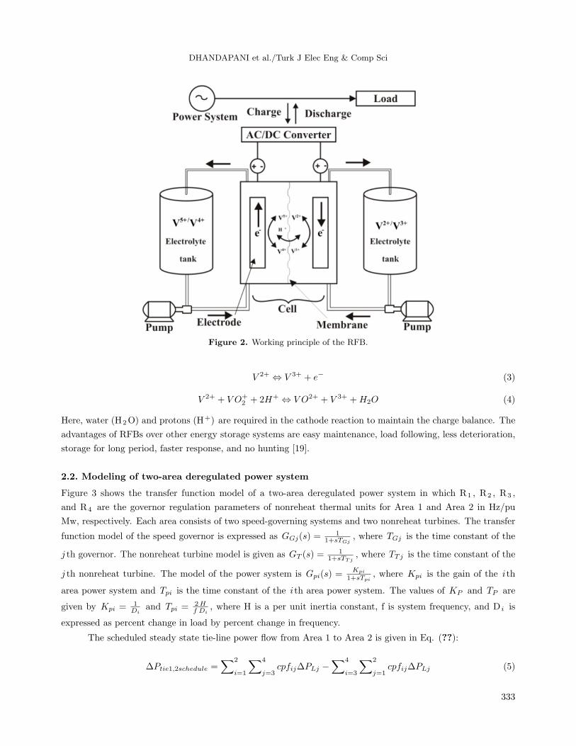
2.1. Principle of RFB operation

A RFB is an electrochemical device that converts electrical energy into chemical energy by means of a reversible

electrochemical reaction. Figure 2 shows the operation principle of a RFB. Vanadium ions (electrolytes)

dissolved in sulfuric acid (H2SO4) are stored in separate tanks and circulated to the battery cell. Eq. (??)

represents the reaction of vanadium redox flow, derived by solving Eqs. (??) and (??).

V O+2 + 2H+ + e− ⇔ V O2+ +H2O (2)

332


Figure 2. Working principle of the RFB.

V 2+ ⇔ V 3+ + e− (3)

V 2+ + V O+2 + 2H+ ⇔ V O2+ + V 3+ +H2O (4)

Here, water (H2O) and protons (H+) are required in the cathode reaction to maintain the charge balance. The

advantages of RFBs over other energy storage systems are easy maintenance, load following, less deterioration,

storage for long period, faster response, and no hunting [19].

2.2. Modeling of two-area deregulated power system

Figure 3 shows the transfer function model of a two-area deregulated power system in which R1 , R2 , R3 ,

and R4 are the governor regulation parameters of nonreheat thermal units for Area 1 and Area 2 in Hz/pu

Mw, respectively. Each area consists of two speed-governing systems and two nonreheat turbines. The transfer

function model of the speed governor is expressed as GGj(s) =1

1+sTGj, where TGj is the time constant of the

j th governor. The nonreheat turbine model is given as GT (s) =1

1+sTTj, where TTj is the time constant of the

j th nonreheat turbine. The model of the power system is Gpi(s) =Kpi

1+sTpi, where Kpi is the gain of the ith

area power system and Tpi is the time constant of the ith area power system. The values of KP and TP are

given by Kpi =1Di

and Tpi =2Hf Di

, where H is a per unit inertia constant, f is system frequency, and D i is

expressed as percent change in load by percent change in frequency.

The scheduled steady state tie-line power flow from Area 1 to Area 2 is given in Eq. (??):

∆Ptie1,2schedule =∑2

i=1

∑4

j=3cpfij∆PLj −

∑4

i=3

∑2

j=1cpfij∆PLj (5)

333


Figure 3. Transfer function model of the deregulated power system.

334


The tie-line power flow from Area 1 to Area 2 is given in Eq. (??):

∆Ptie12actual =2ΠT12

s[∆f1 −∆f2] (6)

Eq. (??) gives the error in the tie-line power flow from Area 1 to Area 2:

∆Ptie12error = ∆Ptie12actual −∆Ptie12schedule (7)

Eq. (??) gives the error in tie-line power flow from Area 2 to Area 1:

∆Ptie21error = a12 ∆Ptie12error (8)

Here, a12 = −Pr1

Pr2, and Pr1 and Pr2 are the rated capacity of Area 1 and Area 2, as both the areas are assumed

to be identical, a12 = −1. The area control error (ACE) of Area 1 and Area 2 is given by Eqs. (??) and (??),

respectively.

ACE1 = B1∆f1 +∆Ptie12error (9)

ACE2 = B2∆f2 + a12∆Ptie12error (10)

As there is more than one Genco in each area, the ACE signal has to be given in proportion to their participation

in LFC. The coefficient that distributes the ACE to all Gencos is known as the ACE participation factor (Apf).

The summation of Apf should always be unity for each area. Hence, the ACE participation factors for Area 1

are Apf11 and Apf12. Similarly, for Area 2, the participation factors are Apf21 and Apf22.

2.3. Modeling of redox flow battery

The RFB is faster than the speed-governing mechanism, as it charges and discharges to suppress the peak value

of frequency deviations quickly against sudden load changes. The RFB is modeled as an active power source

with time constant Trfb and is assumed to be zero, as it is faster than the governor mechanism input [8]. The

transfer function model of RFB in terms of change in power (∆Prfb) is given by Eq. (??).

∆Prfbi =

[Krfbi

1 + sT rfbi

]∆fi (11)

Here, Krfb is the gain of the RFB and Trfb is the time constant of the RFB in seconds.

3. Controllers for load frequency control

If the controllers are not tuned properly, the performance of the system will be poor and possibly unstable. The

conventional PI controller is used and tuning is performed with the trial and error method. The parameters of

the PI are then tuned separately with GA, PSO, and FPA.

3.1. Conventional proportional integral controller

The performance of the proportional controller is good when the rate of change of error is high, which improves

the transient performance. The integral controller is efficient when the error is low, which improves the steady-

state performance. The derivative controller increases the noise and makes the system unstable because of its

335


high sensitivity, although it has the advantage of reducing the overshoot. As the load is subject to change, the

derivative controller makes the system unstable. PI is used due to its simplicity and flexibility. The transfer

function model of PI is given by Eq. (??):

UPI = KPACEi +KI

t∫0

ACEidt (12)

Here, KP is the proportional gain, KI is the integral gain, UPI is the controlled output of the PI controller,

and ACE is the area control error of the area concerned.

3.2. Nature-inspired artificial optimization algorithms

In designing the PI controller, the objective function is defined based on the desired specifications. The proper

parameter setting makes the system stable. The performance index for optimizing the parameters of the PI

controller is defined by using the integral squared error (ISE), given by Eq. (??):

J = ISE =

tsim∫0

(|∆f1|+ |∆f2|+ |∆Ptie1,2|)2dt (13)

where ∆f1 and ∆f2 are the changes in frequency of Area 1 and Area 2, respectively, and ∆P tie1,2 is the

change in tie-line power flow.

The optimal values of the PI controller have been solved using FPA. The performance of the FPA-PI has

been compared with GA-PI and PSO-PI for maximum iterations of 100. The algorithms are explained in the

following sections.

3.2.1. Genetic algorithm

The GA mimics the evolution theory of Darwin. The concept of “survival of the fittest” is used, and the

objective function is converted into a fitness function, control variables as genes, and a collection of genes as

chromosomes. The GA operators are selection, crossover, and mutation. The GA uses multiple points instead

of single-point search and finds the global best value. It optimizes the fitness chromosome through generation

and tunes the genes to the best optimal value through iterations. The set of chromosomes is called a population;

the GA executes each chromosome in the population, keeps the best one, and replaces the unfit chromosome in

each iteration until the global optimal is obtained [20,21]. The procedure of GA is as follows: 1) formulate the

objective function and initialize the chromosome of the population; 2) select the chromosome that survives and

move on to the next generation; 3) cross over a pair of individuals, called parents, to produce two new ones,

called offspring, by exchanging genes; 4) modify the gene values of an existing chromosome. Mutation creates

new chromosomes, thereby increasing the variability of the population.

3.2.2. Particle swarm optimization

PSO is a population-based, biologically inspired optimization technique based on the movement and intelligence

of swarms. The aim of PSO is to find the global optimum fitness function defined in a given search space. It

uses a number of agents (particles) that constitute a swarm, and its position and velocity move in and around

the search space looking for the best solution.

336


Each particle in N-dimensional space adjusts its moving direction and distance according to its own

moving experience, as well as the moving experience of other particles. It keeps track of the coordinates in the

solution space associated with the best solution (fitness) achieved so far by a particle called the personal best

(pbest). Another best value tracked by the PSO is the value obtained so far by any particle in its neighborhood.

This value is called the global best (gbest).

In Eq. (??), c1 and c2 are positive. The acceleration constants, known as social parameters, provide the

correct balance between the individuality and sociality of the particles. r1 and r2 are random numbers that

update each particle’s velocity.

V m+1i = V m

i + c1r1 ∗ (pbesti − dmi ) + c2r2 ∗ (gbest− dmi ) (14)

The position of the particles is updated at each interval, as given by Eq. (??):

dm+1i = dmi + V m+1

i (15)

Here, V i is the velocity of particle I, and Vmi is the modified velocity of particle i at iteration m. Inertia weight

parameter w, which deals with the balancing of the global and local search of PSO, is a positive constant that

lies between 0.5 and 1. By incorporating these parameters in Eq. (??), the updated velocity is given by Eq.

(??).

V m+1i = w ∗ V m

i + c1r1 ∗ (pbesti − dmi ) + c2r2 ∗ (gbest− dmi ) (16)

The procedure is as follows: 1) initialize the number of particles and iterations and design the fitness function;

2) calculate and compare fitness values with their pbest , and if the current value is better than the pbest , then

assign pbest equal to the current value; 3) check the velocity V of each particle; 4) check the particle in the

neighborhood with the best value and assign the coordinates of the best particle as gbest ; 5) update the velocity

and position of each particle; and 6) check for maximum iterations reached and optimal obtained values of gbest

[22].

3.2.3. Flower pollination algorithm

The FPA is a nature-inspired population-based algorithm. Its primary aim is to produce the optimal reproduc-

tion of plant species by survival of the fittest of the flowering plants [23,24]. In this universe, there are millions of

flowering plants, 80% of which are flowering species. The purpose of a flower is to reproduce via pollination, i.e.

the transfer of pollen from one flower to another on the same plant (self-pollination, abiotic) or another plant

(cross-pollination, biotic). This transformation occurs with pollinators such as wind, birds, insects, bats, and

other animals. FPA performs better when compared to other algorithms in terms of accuracy and convergence

speed.

The following four rules were employed to explain the concept of flower pollination: 1) cross-pollination/biotic

are considered as global pollination and the pollinator’s movement, which is similar to the Levy flight movement;

2) local pollination takes place in abiotic and self-pollination environments; 3) pollinators, such as birds and

insects, develop flower constancy, which is equivalent to the reproduction probability and proportional to the

similarity of the two flowers involved; 4) switching from local to global pollination or vice versa can be controlled

with probability P = 0.7.

337


In global pollination, flower pollen is carried by pollinators such as birds, wind, and insects, which travel

over a long distance. This global pollination, i.e. rules 1 and 3, can be written as in Eq. (??):

xk+1i = xk

i + γL (λ)(g∗ − xk

i

)(17)

Here, xki is flower i at iteration k, and g* is the current best solution among the solutions for the current

iteration. γ is the scaling factor used to control the step size and its value is 0.3. L(λ) is the step size

parameter in specific Levy flight movements, which shows the strength of the pollination. As the pollinators

travel over long distances with different movements, Levy distribution is used, as given by Eq. (??):

L ≈ λΓ (λ) sin (πλ/2)

π

1

S1+λ, (S > 0) (18)

Here, Γ (λ) is the standard gamma function. The Levy distribution will be valid for longer steps,

S > 0.

Rules 2 and 3 are for local pollination and are shown in Eq. (??):

xk+1i = xk

i + ε(xkj + xk

m

)(19)

Here, ε is a local random variable, whose values lie between 0 and 1. The flowchart of the tuning of the gain

parameters of PI using the FPA is shown in Figure 4.

4. Case studies

Simulations were carried out in the MATLAB/Simulink environment with 10% load demand on each Disco, as

shown in Figure 3. The test system and RFB parameters used are given in Table 1. The parameters of the GA,

PSO, and FPA are given in Table 2. The proposed deregulated power system model has two Gencos and two

Discos in each area. It has been observed that after a sudden load variation, the system frequency and tie-line

power deviations are disturbed. Hence, in order to suppress the change in area frequency responses and tie-line

power exchanges, the impact of the RFB in both the areas and the controllers is explained below. LFC in a

deregulated power system according to three different scenarios is presented in the following subsections.

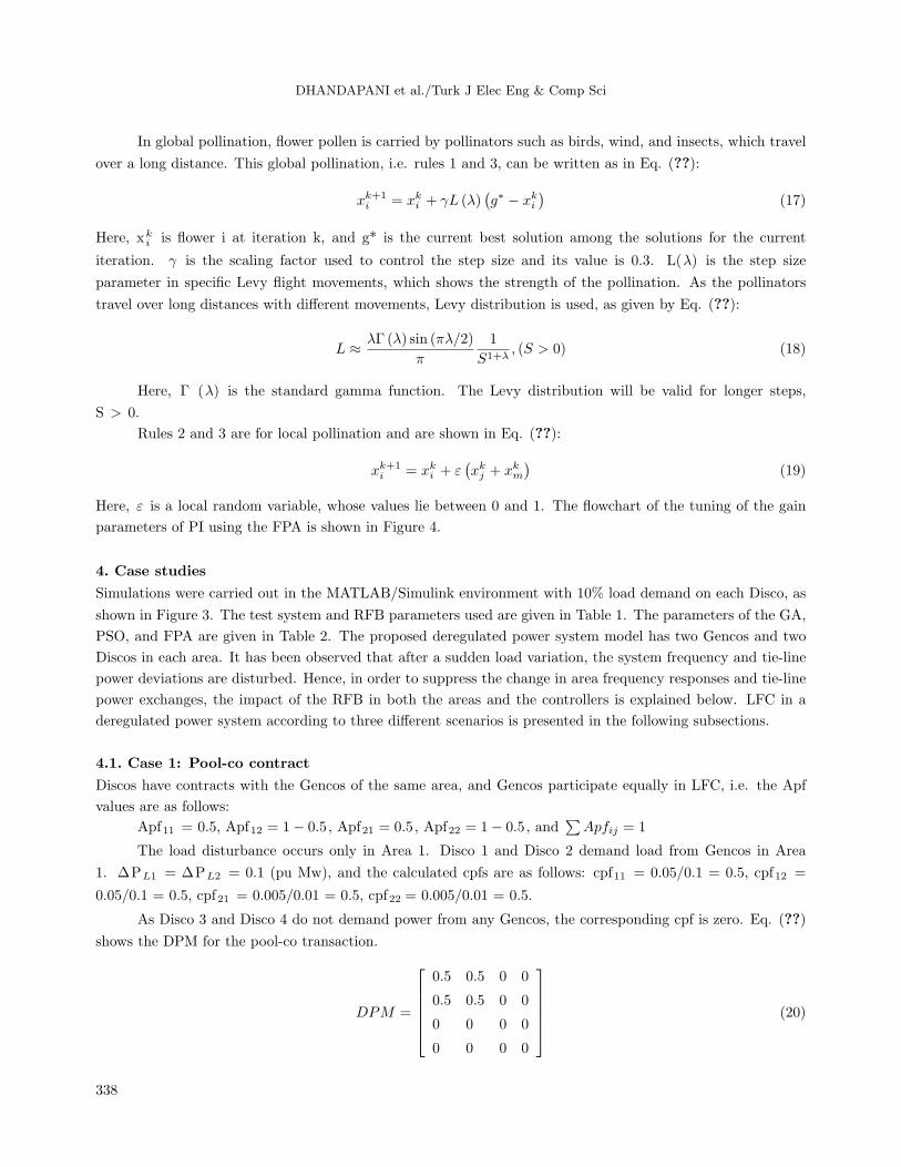
4.1. Case 1: Pool-co contract

Discos have contracts with the Gencos of the same area, and Gencos participate equally in LFC, i.e. the Apf

values are as follows:

Apf11 = 0.5, Apf12 = 1− 0.5, Apf21 = 0.5, Apf22 = 1− 0.5, and∑

Apfij = 1

The load disturbance occurs only in Area 1. Disco 1 and Disco 2 demand load from Gencos in Area

1. ∆PL1 = ∆PL2 = 0.1 (pu Mw), and the calculated cpfs are as follows: cpf11 = 0.05/0.1 = 0.5, cpf12 =

0.05/0.1 = 0.5, cpf21 = 0.005/0.01 = 0.5, cpf22 = 0.005/0.01 = 0.5.

As Disco 3 and Disco 4 do not demand power from any Gencos, the corresponding cpf is zero. Eq. (??)

shows the DPM for the pool-co transaction.

DPM =

0.5 0.5 0 0

0.5 0.5 0 0

0 0 0 0

0 0 0 0

(20)

338


Figure 4. Tuning of PI parameters using the FPA.

339


Table 1. System and RFB parameters.

Parameter (symbol), units ValueRated capacity (Pri), MW 2000Operating load (Pdi), MW 1000Inertia constant (Hi), s 5Regulation droop (Ri), Hz/pu MW 2.5Nominal frequency (f), Hz 60Gain constant of power system (KPi), Hz/pu MW 120Time constant of power system (TPi), s 20Time constant of governor (TGj), s 0.08Time constant of steam turbine (TTj), s 0.3Bias constant (Bi), puMW/Hz 0.425Maximum tie-line capacity (Ptiemax), MW 200Phase angle (δ), degrees 30

Parameter, symbolValue



(units) (units) (units)Damping coefficient,

8.333 × 10−3 Bias factor, Bi 0.425RFB gain

1.8Di (pu Mw/Hz) (pu Mw/Hz) constant, Krfbi

Power system gain120

Tie-line power0.0826

RFB time0

constant, KPi (Hz/pu Mw) constant, T12 constant Trfbi (s)Speed regulation,

2.4Rj (Hz/pu Mw)

Table 2. GA, PSO, and FPA parameters.

GA parameters PSO parameters FPA parametersNumber of chromosomes 20 Number of particles 20 Number of flowers 20Crossover probability 0.25 c1 and c2 2 λ 1.5Mutation probability 0.1 s 0.7

Uncontracted load is considered as zero, i.e. ∆PUC1 = 0 and ∆PUC2 = 0.

Under steady-state conditions, the scheduled tie-line power flow is zero, as in Eq. (??); i.e. the generation

of a Genco should match the demand of the Disco in contract with it. The generated or contracted power supplied

by the Genco is given in Eq. (??):

∆Pgi =4∑

i=1

4∑j=1

cpfij∆PLj (21)

∆Pg1 = cpf11 ∗∆PL1 + cpf12 ∗∆PL2 + cpf13 ∗∆PL3 + cpf14 ∗∆PL4 = 0.1 pu MW.

Similarly, ∆Pg2 = 0.1 pu MW, ∆Pg3 = 0, and ∆Pg4 = 0.

Figures 5a–5c show the dynamic response of change in frequency (Hz) for each area and the tie-line

power flow (pu MW) between them. Tables 3 and 4 give the comparison of controllers in terms of settling time,

overshoot, and undershoot.

340


Figure 5. a) Frequency deviation in Area 1 for pool-co transaction; b) frequency deviation in Area 2 for pool-co

transaction; c) tie-line power deviation for pool-co transaction.

Table 3. Frequency deviation with respect to dynamic response characteristics under three different contract scenarios.

Controller AreaPeak overshoot (Hz) Peak undershoot (Hz) Settling time (s)Case 1 Case 2 Case 3 Case 1 Case 2 Case 3 Case 1 Case 2 Case 3

Frequency deviation (Hz)

PI1 0.015 0.01 0.12 –0.125 –0.27 –0.3 20 44 252 0.6 0.48 0.44 –0.6 –0.75 –0.82 17 28 22

GA-PI1 0.01 0 0 –0.12 –0.14 –0.16 17 19 122 0.3 0.25 0.28 –0.58 –0.62 –0.58 12 12 10

PSO-PI1 0.01 0 0 -0.12 –0.18 –0.18 10 22 102 0.3 0.2 0.18 -0.46 –0.58 –0.58 14 9 12

FPA-PI1 0 0 0 –0.1 0.12 –0.14 5 7 72 0.2 0.15 0.15 –0.4 –0.5 –0.5 6 4 8

4.2. Case 2: Bilateral contract

In this case, a Disco may have a contract with any Genco, either in its own area or in another control area. The

DPM of bilateral contract is given by Eq. (??):

DPM =

0.5 0.25 0.5 0.30.2 0.25 0.2 00 0.25 0.2 0.70.3 0.25 0.1 0

(22)

The Genco participation in LFC is defined by the following Apf values: Apf11 = 0.75, Apf12 = 0.25, Apf21 =

0.5, Apf22 = 0.5, and∑

Apfij = 1.

The demands of Discos (pu MW) are ∆PL1 = ∆PL2 = ∆PL3 = ∆PL4 = 0.1.

341


Table 4. Tie-line power deviation with respect to dynamic response characteristics under three different contract

scenarios.

Controller Area

Peak overshoot (pu MW) Peak undershoot (pu MW) Settling time (s)Case 1 Case 2 Case 3 Case 1 Case 2 Case 3 Case 1 Case 2 Case 3

Tie-line power (pu MW)PI 1–2 1.2 0.24 0.24 –0.3 –0.03 –0.03 32 20 18GA-PI 1–2 1 0.15 0.15 –0.04 –0.02 –0.02 15 15 12PSO-PI 1–2 1 0.14 0.12 –0.02 –0.02 –0.02 17 15 10FPA-PI 1–2 0.7 0.13 0.1 0 –0.02 –0.02 12 12 5

∆PUC1 = 0, ∆PUC2 = 0. Here, the uncontracted load is zero, i.e. there is no contract violation. Under

steady state by using Eq. (??), ∆Ptie1, 2schedule = –0.02 (pu MW).

The power generated by Gencos (pu MW) by using Eq. (??) is as follows:

∆Pg1 = 0.155, ∆Pg2 = 0.065, ∆Pg3 = 0.115, and ∆Pg4 = 0.065.

Figures 6a–6c show the dynamic response of change in frequency (Hz) for each area and the tie-line

power flow (pu MW) between them. Tables 3 and 4 give the comparison of controllers in terms of settling time,

overshoot, and undershoot.

Figure 6. a) Frequency deviation in Area 1 for bilateral transaction; b) frequency deviation in Area 2 for bilateral

transaction; c) tie-line power deviation for bilateral transaction.

4.3. Case 3: Contract violation

In this case, a Disco violates a contract by demanding more power than specified in it. This excess power is not

contracted out to any Genco. It should be supplied by the Gencos in the same area as the Disco and must be

reflected as a local load of the area, not as the contract demand. Consider Case 2 with a modification, where

Disco 3 demands 0.1 pu MW of excess power and the DPM is the same as in Case 2.

342


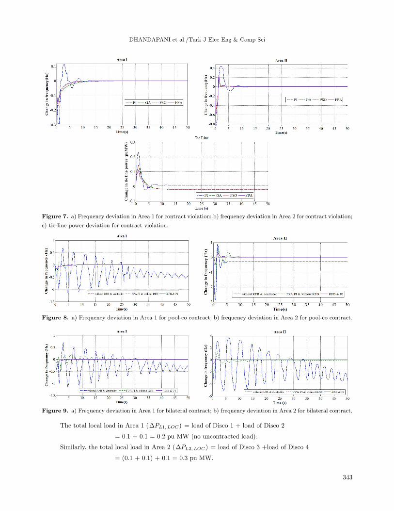
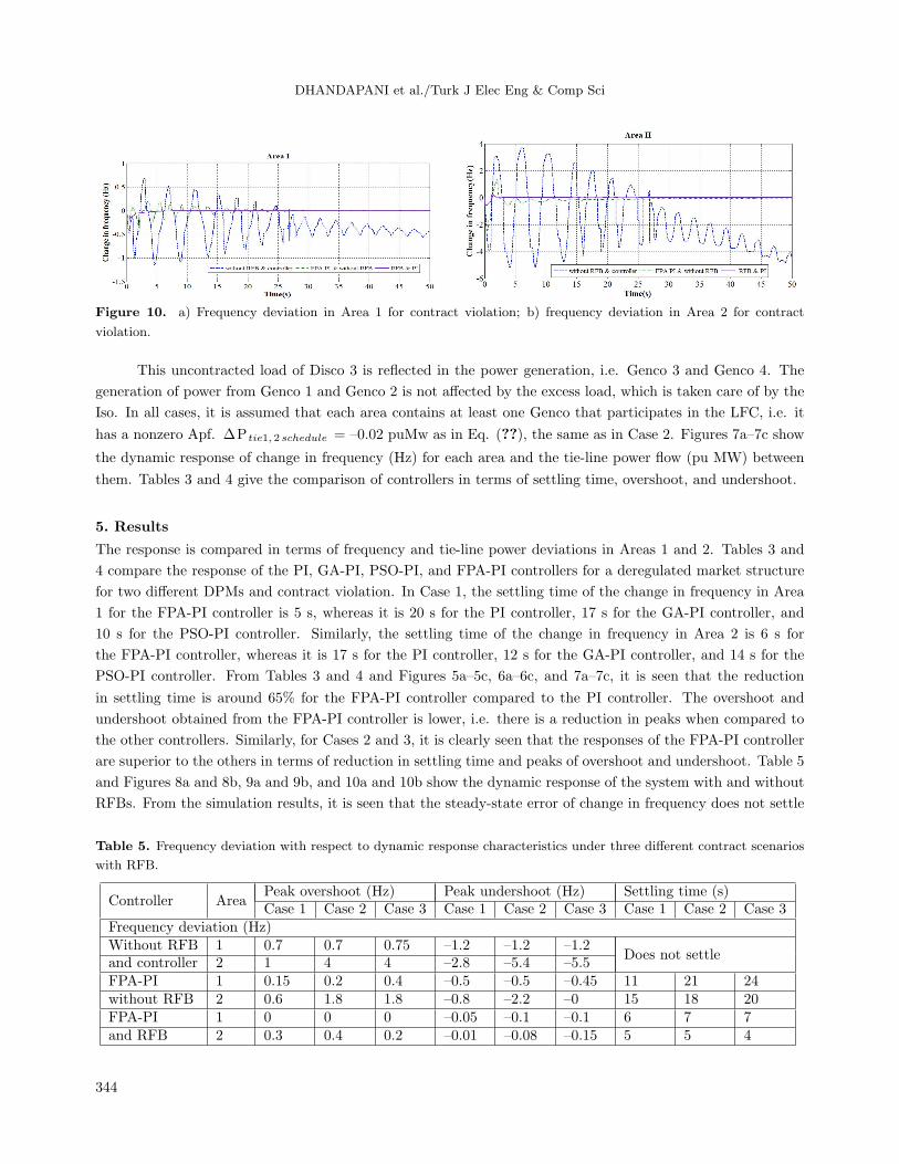
Figure 7. a) Frequency deviation in Area 1 for contract violation; b) frequency deviation in Area 2 for contract violation;

c) tie-line power deviation for contract violation.

Figure 8. a) Frequency deviation in Area 1 for pool-co contract; b) frequency deviation in Area 2 for pool-co contract.

Figure 9. a) Frequency deviation in Area 1 for bilateral contract; b) frequency deviation in Area 2 for bilateral contract.

The total local load in Area 1 (∆PL1, LOC) = load of Disco 1 + load of Disco 2

= 0.1 + 0.1 = 0.2 pu MW (no uncontracted load).

Similarly, the total local load in Area 2 (∆PL2, LOC) = load of Disco 3 +load of Disco 4

= (0.1 + 0.1) + 0.1 = 0.3 pu MW.

343


Figure 10. a) Frequency deviation in Area 1 for contract violation; b) frequency deviation in Area 2 for contract

violation.

This uncontracted load of Disco 3 is reflected in the power generation, i.e. Genco 3 and Genco 4. The

generation of power from Genco 1 and Genco 2 is not affected by the excess load, which is taken care of by the

Iso. In all cases, it is assumed that each area contains at least one Genco that participates in the LFC, i.e. it

has a nonzero Apf. ∆P tie1, 2 schedule = –0.02 puMw as in Eq. (??), the same as in Case 2. Figures 7a–7c show

the dynamic response of change in frequency (Hz) for each area and the tie-line power flow (pu MW) between

them. Tables 3 and 4 give the comparison of controllers in terms of settling time, overshoot, and undershoot.

5. Results

The response is compared in terms of frequency and tie-line power deviations in Areas 1 and 2. Tables 3 and

4 compare the response of the PI, GA-PI, PSO-PI, and FPA-PI controllers for a deregulated market structure

for two different DPMs and contract violation. In Case 1, the settling time of the change in frequency in Area

1 for the FPA-PI controller is 5 s, whereas it is 20 s for the PI controller, 17 s for the GA-PI controller, and

10 s for the PSO-PI controller. Similarly, the settling time of the change in frequency in Area 2 is 6 s for

the FPA-PI controller, whereas it is 17 s for the PI controller, 12 s for the GA-PI controller, and 14 s for the

PSO-PI controller. From Tables 3 and 4 and Figures 5a–5c, 6a–6c, and 7a–7c, it is seen that the reduction

in settling time is around 65% for the FPA-PI controller compared to the PI controller. The overshoot and

undershoot obtained from the FPA-PI controller is lower, i.e. there is a reduction in peaks when compared to

the other controllers. Similarly, for Cases 2 and 3, it is clearly seen that the responses of the FPA-PI controller

are superior to the others in terms of reduction in settling time and peaks of overshoot and undershoot. Table 5

and Figures 8a and 8b, 9a and 9b, and 10a and 10b show the dynamic response of the system with and without

RFBs. From the simulation results, it is seen that the steady-state error of change in frequency does not settle

Table 5. Frequency deviation with respect to dynamic response characteristics under three different contract scenarios

with RFB.

Controller AreaPeak overshoot (Hz) Peak undershoot (Hz) Settling time (s)Case 1 Case 2 Case 3 Case 1 Case 2 Case 3 Case 1 Case 2 Case 3

Frequency deviation (Hz)Without RFB 1 0.7 0.7 0.75 –1.2 –1.2 –1.2

Does not settleand controller 2 1 4 4 –2.8 –5.4 –5.5FPA-PI 1 0.15 0.2 0.4 –0.5 –0.5 –0.45 11 21 24without RFB 2 0.6 1.8 1.8 –0.8 –2.2 –0 15 18 20FPA-PI 1 0 0 0 –0.05 –0.1 –0.1 6 7 7and RFB 2 0.3 0.4 0.2 –0.01 –0.08 –0.15 5 5 4

344


at zero when the RFB is not included. However, in the presence of the RFB and the controller, the response is

faster with reduced oscillations and the system settles at zero. From Tables 3 and 4 it is seen that the FPA-PI

controller gives a better response than the others.

6. Conclusion

In this work, the FPA-PI controller for LFC of a two-area deregulated power system is designed and its

performance is analyzed. The integral square error is used as the objective function for the optimization of

the controller parameters using heuristic optimization techniques. The FPA-PI is compared with GA-PI and

PSO-PI. The results show that the FPA-PI gives better performance in terms of settling time, overshoot, and

undershoot when compared to the other techniques. Furthermore, in order to improve the overall response of

the system, RFBs are added to the two areas. This reduces the time delay due to the slow response of the speed

governor. Therefore, it has been proven that the performance of the FPA-PI controller with a RFB is better

than the conventional PI controller in terms of peak overshoot, peak undershoot, and settling time.

References

[1] Elgerd OI. Electric Energy Systems Theory: An Introduction. 2nd ed. New York, NY, USA: McGraw-Hill, 1983.

[2] Kumar J, Ng KH, Sheble G. AGC simulator for price-based operation part I. IEEE T Power Syst 1997; 12: 527-532.

[3] Christie RD, Bose A. Load frequency control issues in power system operation after deregulation. IEEE T Power

Syst 1996; 11: 1191-1200.

[4] Aditya SK, Das D. Battery energy storage for load frequency control of an interconnected power system. Electr

Pow Syst Res 2001; 58: 179-185.

[5] Kumar SR, Ganapathy S. Impact of energy storage units on load frequency control of deregulated power systems.

Energy 2016; 97: 214-228.

[6] Pappachen A, Fathima AP. Load frequency control in deregulated power system integrated with SMES–TCPS

combination using ANFIS controller. Int J Elec Power 2016; 82: 519-534.

[7] Sasaki T, Kadoya T, Enomoto K. Study on load frequency control using redox flow batteries. IEEE T Power Syst

2004; 19: 660-667.

[8] Chidambaram IA, Paramasivam B. Optimized load-frequency simulation in restructured power system with redox

flow batteries and interline power flow controller. Int J Elec Power 2013; 50: 9-24.

[9] Donde V, Pai MA, Hiskens IA. Simulation and optimization in an AGC system after deregulation. IEEE T Power

Syst 2001; 16: 481-489.

[10] Shayeghi H, Shayanfar HA, Jalili A. Load frequency control strategies: a state-of-the-art survey for the researcher.

Energ Convers Manage 2009; 50: 344-353.

[11] Tyagi B, Srivastava SC. A LQG-based load frequency controller in a competitive electricity environment. Int J

Emerg Electr Power Syst 2005; 2: 1-13.

[12] Dola GP, Somanath M. A new control scheme for PID controller of single-area and multi-area power systems. ISA

T 2013; 52: 242-251.

[13] Zamani AA, Bijami E, Sheikholeslam F, Jafrasteh B. Optimal fuzzy load frequency controller with simultaneous

auto-tuned membership functions and fuzzy control rules. Turk J Elec Eng & Comp Sci 2014; 22: 66-86.

[14] Demiroren A, Zeynelgil HL. GA application to optimization of AGC in three-area power system after deregulation.

Int J Elec Power 2007; 29: 230-240.

[15] Bhatt P, Roy R, Ghoshal SP. Optimized multi area AGC simulation in restructured power systems. Int J Elec

Power 2010; 32: 311-332.

345

http://dx.doi.org/10.1109/59.589593

http://dx.doi.org/10.1109/59.535590

http://dx.doi.org/10.1109/59.535590

http://dx.doi.org/10.1016/S0378-7796(01)00129-8

http://dx.doi.org/10.1016/S0378-7796(01)00129-8

http://dx.doi.org/10.1016/j.ijepes.2016.04.032


http://dx.doi.org/10.1109/TPWRS.2003.818724

http://dx.doi.org/10.1109/TPWRS.2003.818724



http://dx.doi.org/10.1109/59.932285

http://dx.doi.org/10.1109/59.932285

http://dx.doi.org/10.1016/j.enconman.2008.09.014

http://dx.doi.org/10.1016/j.enconman.2008.09.014

http://dx.doi.org/10.3906/elk-1203-3







[16] Kumar N, Kumar V, Tyagi B. Optimization of PID parameters using BBBC for a multiarea AGC scheme in a

deregulated power system. Turk J Elec Eng & Comp Sci 2016; 24: 4105-4116.

[17] Kumar N, Kumar V, Tyagi B. Deregulated multiarea AGC scheme using BBBC-FOPID controller. Arab J Sci Eng

2016; 42: 2641-2649.

[18] Fathima AP, Khan MA. Design of new market structure and robust controller for the frequency regulation service

in the deregulated power system. Electr Pow Compo Sys 2008; 33: 864-883.

[19] Weber AZ, Matthew MM, Jeremy PM, Philip NR, Jeffery T, Gostick QL. Redox flow batteries. J Appl Electrochem

2011; 41: 1137-1164.

[20] Yang XS. Engineering Optimization: An Introduction with Metaheuristic Applications. New York, NY, USA: Wiley,

2010.

[21] Magid YLA, Dawoud MM. Optimal AGC tuning with genetic algorithms. Electr Pow Syst Res 1996; 38: 231-238.

[22] Kennedy J, Eberhart R. Swarm Intelligence. San Diego, CA, USA: Academic Press, 2001.

[23] Glover BJ. Understanding Flowers and Flowering: An Integrated Approach. Oxford, UK: Oxford University Press,

2007.

[24] Yang XS. Engineering Optimization: An Introduction with Metaheuristic Application. New York, NY, USA: Wiley,

2010.

346



http://dx.doi.org/10.1007/s13369-016-2293-1

http://dx.doi.org/10.1007/s13369-016-2293-1

http://dx.doi.org/10.1007/s10800-011-0348-2

http://dx.doi.org/10.1007/s10800-011-0348-2

http://dx.doi.org/10.1016/S0378-7796(96)01091-7

two-area load frequency control with redox ow battery using...

Documents