tutorial from sample to analyzed data using qiime for analysis
TRANSCRIPT

1
Metagenomics Workshop Led by Regina Lamendella, Juniata College
[email protected] 814-641-3553
Acknowledgements: I would like to thank Abigail Rosenberger, Alyssa Grube, Colin Brislawn, and Erin McClure for developing many of these tutorials preparing this document
Table of Contents MODULE 1: PREPARATION OF MICROBIAL SAMPLES FOR HIGH THROUGHPUT SEQUENCING
Background Module Goals V&C Core Competencies GCAT-SEEK Sequencing Requirements Instrumentation and Supply Requirements Protocols
A. Library Preparation 1. 16S rRNA gene Illumina tag (itag) PCR 2. ITS Illumina tag (itag) PCR
B. Check PCR Amplification 1. Pool replicate samples 2. E-gel electrophoresis 3. DNA quantification with the Qubit fluorometer a. Introduction b. Materials c. Protocol C. Quality Check Libraries 1. Pool samples 2. Gel electrophoresis 3. QIAquick gel purification 4. Bioanalyzer a. Introduction b. Agilent High Sensitivity DNA assay protocol c. Interpreting Bioanalyzer results Assessments Module Timeline Discussion Topics for class Applications in the classroom References and Suggested Reading
MODULE 2: SEQUENCE ANALYSIS
Background

2
Module Goals V & C Core Competencies GCAT-SEEK Sequencing Requirements Computer/Program Requirements Protocols
A. Unix/Linux Tutorial B. Thinking about your biological question(s) C. Introduction to QIIME D. Getting QIIME E. Installing the QIIME VirtualBox image F. QIIME 16S Workflow 1. Conventions 2. Flowchart 3. Metadata 4. Extract compressed files 5. Split libraries workaround 6. OTU table picking 7. Initial analyses a. OTU table statistics b. Clean OTU table c. Summarize taxa 8. Diversity analyses a. Alpha diversity b. Beta diversity 9. Statistical analyses a. OTU category significance b. Compare categories c. Compare alpha diversity 10. Heatmaps G. QIIME Fungal ITS Workflow 1. Obtain tutorial files 2. OTU picking
Assessments Applications in the classroom Module Timeline Discussion Topics for class References and Suggested Reading
APPENDIX A. Primers B. Helpful links C. Additional protocols/scripts 1. Purification by SPRI beads 2. DNA Precipitation 3. Splitting libraries – the traditional method D. Other software

3
1. Installing R 2. Proprietary software for data analysis E. Computing 1. Troubleshooting error messages 2. Connecting to the GCAT-SEEK server 3. Connecting to Juniata’s HHMI Cluster 4. IPython Notebook 5. Bash scripting

4
MODULE 1: PREPARATION OF MICROBIAL SAMPLES FOR HIGH-THROUGHPUT SEQUENCING
After this module you will be able to show your children how to do this…I promise!
Background
The term ‘metagenomics’ was originally coined by Jo Handelsman in the late 1990s and is currently defined as the application of modern genomics techniques to the study of microbial communities directly in their natural environments”. The culture-independent molecular techniques have allowed microbiologists to tap into the vast microbial diversity of our world. Recently, massively parallel, high-throughput sequencing (HTS) has enabled taxonomic profiling of microbial communities to become cost-effective and informative. Initiatives such as the Earth Microbiome Project, the Hospital Microbiome Project, the Human Microbiome Project, and others are consortia tasked with uncovering the distribution of microorganisms within us and our world. Many efforts have focused on probing regions of the ribosomal RNA operon as a method for ‘telling us who is there in our sample”. The rRNA operon contains genes encoding structural and functional portions of the ribosome. This operon contains both highly conserved and highly variable regions, which allow microbial ecologists to both simultaneously target and distinguish diverse taxa in a sample. Microbiologists have relied upon DNA sequence information for microbial identification, based primarily on the gene encoding the small subunit RNA molecule of the ribosome (16S rRNA gene). Databases of rRNA sequence data can be used to design phylogenetically conserved probes that target both individual and closely related groups of microorganisms without cultivation. Some of the most well curated databases of 16S rRNA sequences include Greengenes, the Ribosomal Database Project, and ARB-Silva (see references section for links to these databases).
Figure 1. Structure of the rRNA operon in bacteria. Figure from Principles of Biochemistry 4th Edition Pearson Prentice Hall Inc. 2006
5
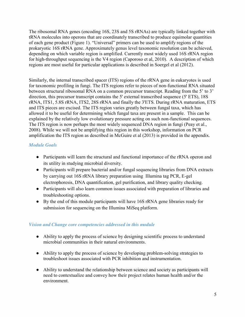
The ribosomal RNA genes (encoding 16S, 23S and 5S rRNAs) are typically linked together with tRNA molecules into operons that are coordinately transcribed to produce equimolar quantities of each gene product (Figure 1). “Universal” primers can be used to amplify regions of the prokaryotic 16S rRNA gene. Approximately genus level taxonomic resolution can be achieved, depending on which variable region is amplified. Currently most widely used 16S rRNA region for high-throughput sequencing is the V4 region (Caporoso et al, 2010). A description of which regions are most useful for particular applications is described in Soergel et al (2012).
Similarly, the internal transcribed spacer (ITS) regions of the rRNA gene in eukaryotes is used for taxonomic profiling in fungi. The ITS regions refer to pieces of non-functional RNA situated between structural ribosomal RNA on a common precursor transcript. Reading from the 5’ to 3’ direction, this precursor transcript contains the 5' external transcribed sequence (5' ETS), 18S rRNA, ITS1, 5.8S rRNA, ITS2, 28S rRNA and finally the 3'ETS. During rRNA maturation, ETS and ITS pieces are excised. The ITS region varies greatly between fungal taxa, which has allowed it to be useful for determining which fungal taxa are present in a sample. This can be explained by the relatively low evolutionary pressure acting on such non-functional sequences. The ITS region is now perhaps the most widely sequenced DNA region in fungi (Peay et al., 2008). While we will not be amplifying this region in this workshop, information on PCR amplification the ITS region as described in McGuire et al (2013) is provided in the appendix.
Module Goals
Participants will learn the structural and functional importance of the rRNA operon and its utility in studying microbial diversity.
Participants will prepare bacterial and/or fungal sequencing libraries from DNA extracts by carrying out 16S rRNA library preparation using Illumina tag PCR, E-gel electrophoresis, DNA quantification, gel purification, and library quality checking.
Participants will also learn common issues associated with preparation of libraries and troubleshooting options.
By the end of this module participants will have 16S rRNA gene libraries ready for submission for sequencing on the Illumina MiSeq platform.
Vision and Change core competencies addressed in this module
Ability to apply the process of science by designing scientific process to understand microbial communities in their natural environments.
Ability to apply the process of science by developing problem-solving strategies to
troubleshoot issues associated with PCR inhibition and instrumentation.
Ability to understand the relationship between science and society as participants will need to contextualize and convey how their project relates human health and/or the environment.

6
Ability to tap into the interdisciplinary nature of science by applying physical and
chemical principles of molecules to provide an in depth understanding of high-throughput sequencing technologies.
GCAT-SEEK sequencing requirements
The libraries will be sequenced using the Illumina MiSeq platform. This technology currently yields up to 300 bp read lengths. Single end runs yield 12-15 million reads, while paired end read lengths yield 24-30 million reads. More information is available at:
Video: http://www.youtube.com/watch?v=t0akxx8Dwsk Background Information: http://www.youtube.com/watch?v=t0akxx8Dwsk
Our prepared libraries for this workshop will be sequenced at the Dana Farber Sequencing Center. They offer full MiSeq runs for $1,000 for educational research purposes. http://pcpgm.partners.org/research-services/sequencing/illumina
The BROAD Institute provides a great set of Illumina sequencing videos, which are really in-depth and helpful. Visit: http://www.broadinstitute.org/scientific-community/science/platforms/genome-sequencing/broadillumina-genome-analyzer-boot-camp
Instrumentation and supply requirements for this module
1) Pipettes and tips
For projects with more than 48 samples, multi-channel pipettes are helpful!
2) Qubit fluorometer- Life technologies, more information at: http://www.invitrogen.com/site/us/en/home/brands/Product-Brand/Qubit.html Note: The PicoGreen assay and a Spec reader is just as accurate as the Qubit 2.0 fluorometer. Nanodrop or specs that read 260/280 ratio can be used, but are not as accurate because other substances can absorb at the same wavelength as DNA and skew results.
3) Thermocycler - pretty much any one will do. At Juniata we use a mix of BIO-RAD’s and MJ Research cyclers.
4) Electrophoresis unit- Any electrophoresis unit will work fine. We typically use between 1-2% agarose gels for all applications. We stain our gels with GelStar GEL STAIN. Ethidium bromide is fine too. Any 1Kb ladder will suffice.
For the initial check gel after PCR, we use the high-throughput E-gel system by Life Technologies to save time in the classroom. The gels are bufferless, precast, and only

7
take 12 minutes to run! More information on the Egel system can be found at http://www.invitrogen.com/site/us/en/home/Products-and-Services/Applications/DNA-RNA-Purification-Analysis/Nucleic-Acid-Gel-Electrophoresis/E-Gel-Electrophoresis-System
5) PCR reagents: TaKaRa Ex Tax is what we use for the PCR reagents in this module. 6) Primers used in this study were ordered from IDT. These primers were ordered in a 96-
well format and were normalized to 3 nanomoles. The approximate cost is 28 cents per basepair. So each plate of primers costs roughly $2,000 USD. Call your regional IDT rep and they will give you a sizeable discount. More information can be found at http://www.earthmicrobiome.org/emp-standard-protocols/16s/
7)
Luckily we have tons of bacterial primers so that we can send aliquots of them directly to you, if needed.
A list of the primer constructs used in this module can be found in the Appendix.
8) Gel visualization apparatus. Any type of UV box with a camera adaptor will work.
9) Bioanalyzer 2100 and Expert software. More information on the Bioanalyzer is available at: https://www.genomics.agilent.com/article.jsp?pageId=275
If you don’t have a Bioanalyzer, any sequencing facility can quality check your libraries for you for a small additional cost (roughly 100-150$/chip).

8
Table 1. List of reagents used in this module
Company order number Description price 2014
Lonza 50535 GelStar GEL STAIN 10,000 0X (2 X 250uL) $161.00
TaKaRa Ex Taq RR001A TaKaRa Ex Taq® DNA Polymerase (250) $169.00
Qiagen 28604 MinElute Gel Extraction Kit (50) $117.00
IDT get quote each primer is 68 bp x 28 cents/ base x 96 primers per plate $1,827.84
Life Technologies G7008-02 2% E-Gel® 96 Agarose $219.00 Life Technologies 12373031 Egel low range ladder $94.00 Agilent 5067-1504 Agilent DNA 1000 Kit (25 chips) $773.00

9
Protocols
Some of protocols have been adapted from the Earth Microbiome Project. For further information please visit: http://www.earthmicrobiome.org/
A. Library Preparation
16S rRNA gene Illumina tag (itag) PCR (set up time 2 hours, runtime 3 hours)
Illumina tag PCR amplification accomplishes two steps in one reaction. The desired region(s) of the 16S rRNA gene is amplified, which is typically required to obtain enough DNA for sequencing. By modifying the primer constructs to include the Illumina adapters and a unique barcode, the amplified region of the 16S rRNA gene can be identified in a pooled sample and the sample is prepared for sequencing with the Illumina MiSeq platform.
Figure 2. Protocol for barcoded Illumina sequencing. A target gene is identified, which in this case is the V4 region of the 16S rRNA gene. This region is PCR amplified using primer constructs with Illumina adapters, linker and pad sequences, and the forward/reverse primers themselves. The reverse primer construct contains an additional 12 bp barcode sequence. After

10
PCR amplification, the target region is labeled with Illumina adapters and the barcode. The sequencing primers anneal and produce reads, while the index sequencing primer sequences the barcode. This information is used prior to analyzing the reads to demultiplex the sequences. See Caporaso et al (2011) for more information.
These PCR amplification protocols are based on the Earth Microbiome Project’s list of standard protocols. (http://www.earthmicrobiome.org/emp-standard-protocols/16s/)
PCR Conditions
Reactions will be performed in duplicate. Record the PCR plate set up in the appropriate spreadsheet. Table 2. Components of the PCR reaction for 16S rRNA gene amplification.
Reagent [Initial]
Volume (μL)
[Final] Num. Rxns
Amount
TaKaRa Ex Taq MM
2X 5.625 1X
DNA template X Reverse primer 5 μM 1.0 0.2 μM PCR grade H2O X
Total volume 25.0
The master mix provided contains the TaKaRa Ex Taq (0.125 μL), 10X Ex Taq Buffer (2.5 μL), dNTP Mixture (2 μL), forward primer (1μL), and PCR grade H2O. Add 23 μLof the provided master mix, 1.0 μL reverse primer, and 1.0 μL template into each well.
When making negative controls, use 1.0 μl PCR grade H2O instead of the template. Between 5% and 10% of the samples should be negative controls if space permits.
When setting up your own reactions, use the last two columns to determine how much of each component you will need given the total number of samples and negative controls. Then aliquot 23 μl of this master mix into each well and add the unique components afterward.
On the next page there is a blank table. As you set up your reactions, list the sample you are putting in each well on this sheet. This works best if you work in pairs. One partner will pipette, and the other partner will record what sample is being put in a given well. Lastly, be sure to put the reverse primer A1 in the reaction you put in cell A1, reverse primer A2 in the reaction you put in cell A2, and so on.

11
DO NOT LOSE THIS PAPER! If you lose this paper you will have no way of tracking your samples after PCR, and consequently will be kicked out of the workshop. (Not really, but DO NOT LOSE THIS PAPER.)

12
Thermocycling Conditions
1. 94°C for 3 min to denature the DNA 2. 94 °C for 45 s 3. 50 °C for 60 s 4. 72 °C for 90 s 5. 72 °C for 10 min for final extension 6. 4 °C HOLD
B. Check PCR Amplification (1-2 hours)
1. Pooling the DNA (30 mins- 1hour depending on the number of samples)
Combine duplicate reactions into a single pool per sample. After combining, determine which PCR reactions were successful with the E-gel electrophoresis protocol.
2. E-Gel Electrophoresis (15-30 mins for loading; 15 mins for runtime)
E-Gels can be used to check the PCR product instead of traditional gel electrophoresis. We will only combine the successfully amplified samples for sequencing. We can also detect the presence of additional bands in the reactions, which may signal amplification of chloroplast DNA or excessive primer dimer bands. If these bands are present, we will need to purify the desired band from a traditional agarose gel.
The gels come pre-stained with EtBr or SYBR, and are encased in plastic. Buffer is already included, and the gels run rapidly (~ 12 min). The E-gel electrophoresis unit and a specific ladder are required.
1. Combine 16 μl diH20 and 4 μl PCR product.
2. Remove the comb from the gel.
3. Load into E gel wells. Load 20 μl diH20 into empty wells (including unused marker).
4. Load 10 μl low range ladder and 10 μl diH2O into the marker wells.
5. Depending on the gel base, choose the proper program if available and begin electrophoresis.
6. Run for the specified amount of time.
7. Remove E gel and image in UV box.
16S rRNA gene products will be roughly 300-350 bp.
8. Record successful reactions on the E-gel layout spreadsheet.

13
3. DNA Quantification with the Qubit fluorometer (Sample dependent about 90 mins for 96 samples)
a. Introduction
The Qubit system was designed to specifically quantify nucleic acids and proteins using small quantities of PCR product. The fluorescent probe (Qubit reagent) intercalates double stranded DNA (dsDNA) and fluoresces only after intercalation. Other methods of DNA quantification rely on UV-Vis spectroscopy to quantify nucleic acids; however they are much less specific as the dsDNA, RNA, and proteins absorb overlapping wavelengths. Since the fluorophore fluoresces only after intercalating dsDNA, the DNA concentrations assayed with the Qubit system are much more accurate than with other methods. See the Qubit 2.0 user manual and the Invitrogen website for more information.
(http://www.invitrogen.com/etc/medialib/en/filelibrary/cell_tissue_analysis/Qubit-all-file-types.Par.0519.File.dat/Qubit-2-Fluorometer-User-Manual.pdf)
(http://www.invitrogen.com/site/us/en/home/brands/Product-Brand/Qubit/qubit-fluorometer.html)
Figure 3. The fluorescent probe (blue) intercalates the dsDNA, allowing for both precise measurement of the dsDNA concentration of a sample. For more information, see the Invitrogen website. (http://www.invitrogen.com/site/us/en/home/Products-and-Services/Applications/DNA-RNA-Purification-Analysis.html)
14
b. Materials
Qubit Fluorometer
Qubit dsDNA HS Buffer
Qubit reagent (protect from light)
Qubit Assay tubes
Standards 1 and 2, concentrations of 0ng and 10ng respectively
DNA extract or PCR Product
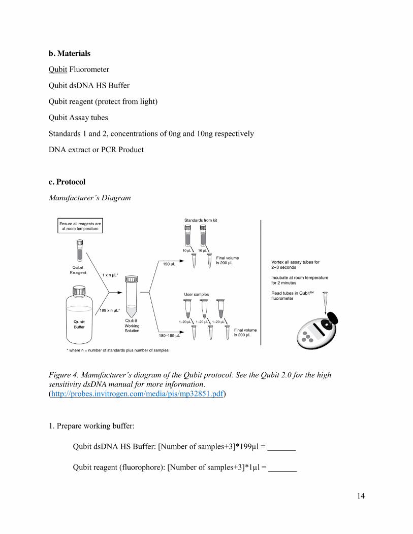
c. Protocol
Manufacturer’s Diagram
Figure 4. Manufacturer’s diagram of the Qubit protocol. See the Qubit 2.0 for the high sensitivity dsDNA manual for more information. (http://probes.invitrogen.com/media/pis/mp32851.pdf)
1. Prepare working buffer:
Qubit dsDNA HS Buffer: [Number of samples+3]*199µl = _______
Qubit reagent (fluorophore): [Number of samples+3]*1µl = _______

15
Note: The extra 3 samples allow for 2 standards and for pipetting error
2. Vortex the working buffer to mix
3. Label Qubit Assay tubes with sample ID
4. For each sample, add 2µl of PCR product to 198µl of working buffer to the appropriate tube
5. For each of the two standards, add 10µl of standard to 190µl of working buffer to the
appropriate tube
6. Vortex each sample for 2-3 seconds to mix
7. Incubate for 2 minutes at room temperature
8. On the Qubit fluorometer, hit DNA, then dsDNA High Sensitivity, then YES.
9. When directed, insert standard 1, close the lid, and hit Read
10. Repeat step 9 for standard 2. This produces your two-point standard calibration.
11. Read each sample by inserting the tube into the fluorometer, closing the lid, and hitting Read
Next Sample
12. Use the spreadsheet dna_quants.xlsx to record the data.
C. Quality Check Libraries
1. Pool 240 ng DNA per sample into one collection tube (one hour)
See the column “Volume to pool” in the spreadsheet dna_quants.xlsx for the volume of each sample to add to the pool.
2. Gel Electrophoresis (prep 90 mins; loading and runtime 90 mins) (not at workshop)
There may be extra bands in the PCR product caused by amplification of chloroplast DNA, primer dimers, or other undesired amplification. You can separate the desired band from the unwanted bands by traditional gel electrophoresis and gel purification.

16
1. Tape up gel tray or use rubber gasket to seal.
2. Place comb in gel tray.
3. Make a 1.5% (35 ml, depends on box size) agarose gel with 1X TBE buffer.
4. Cool gel solution on a stir plate until you can touch the glass
5. Add 4 μl Gelstar (SYBR green based) per 100 ml gel to the gel right before you pour.
6. Pour gel slowly from one corner. Avoid introducing air bubbles as you pour.
7. Let gel cool for between 1 and 1.5 hours. Remove tape and place into gel rig.
8. Make 250 ml 0.5X TBE running buffer (depends on box size). Make sure it’s enough to cover
gel.
9. Load 3 ul 6X loading dye (Affymetrix) into each well of a 96 well plate.
11. Load 15 ul PCR product into each well of the same 96 well plate.
12. Remove comb gently from gel.
13. Load 5 ul ladder (1kb Plus, Affymetrix).
14. Load all 15 ul PCR product/loading dye into the wells.
15. Run gel for about 1.5 to 2 hrs at between 60-80V.
3. QIAquick Gel Purification (2 hours) (not at workshop)
1. Excise the DNA fragments from the agarose gel with a clean, sharp scalpel- - Minimize the size of the gel slice by removing extra agarose
** minimize light exposure and manipulation of gel as this can denature the DNA**
*** ALWAYS wear safety glasses and keep the cover on the gel when looking on the light***
2. Weigh the gel slice in a colorless tube. Add 3 volumes of Buffer QG to 1 volume of gel.

17
- E.g. a 100 mg gel slice would require 300 PL of Buffer QG. The maximum amount of gel slice per QIAquick column in 400 mg. For a gel slice > 400 mg use more than one QIAquick column.
3. Incubate at 50⁰C for 10 minutes or until gel slice is completely dissolved. Can vortex to help dissolve gel mixture.
4. After gel slice is dissolved completely, check that the color of the mixture is yellow. If it is orange or violet, add 10 PL of 3 M sodium acetate, pH5 and mix. This should bring the mixture back to yellow.
5. Add 1 gel volume of isopropanol (or 200 proof EtOH) to the sample and mix. 6. Place a QIAquick spin column in a 2 mL collection tube 7. To bind DNA, apply the sample to the QIAquick column and centrifuge 1 minute. The
maximum reservoir or the column is 800 PL. For samples greater than 800 P just load and spin again.
8. Discard flow through and place column back in same collection tube. 9. Add 0.5 mL of buffer QG and centrifuge for 1 min. 10. To wash: add 0.75 mL buffer PE to QIAquick column and centrifuge 1 min. 11. Discard flow through and centrifuge for an additional 1 minute at 17,900g (13,000 rpm) 12. Place QIAquick column into a clean, labeled, 1.5 mL microcentrifuge tube 13. To elute DNA, add 30 PL of Buffer EB to the center of the QIAquick membrane and
centrifuge for 1 minute. Take flow-through and spin through the column again. Discard column.
14. Freeze products.
4. Bioanalyzer (Not included workshop activities)
a. Introduction
The Bioanalyzer (Agilent) is used to assess the quality of the pooled DNA before it is sent to the sequencing core. The Bioanalyzer uses microfluidics technology to carry out gel electrophoresis on a very small scale. A gel-dye mix is prepared and spread into the wells of the chip during the chip priming step. Marker, the ladder, and the samples are loaded and the chip is vortexed briefly. During the run, the DNA fragments migrate and are compared to the migration of the ladder, resulting in a precise calculation of DNA fragment size and abundance. The Bioanalyzer works with RNA as well, and is useful for determining the quality of RNA. See the DNA assay protocol and the Agilent website for more information about the applications and troubleshooting guides.
http://www.chem.agilent.com/library/usermanuals/Public/G2938-90014_KitGuideDNA1000Assay_ebook.pdf

18
http://www.genomics.agilent.com/en/Bioanalyzer-Instruments-Software/2100-Bioanalyzer/?cid=AG-PT-106&tabId=AG-PR-1001
b. Agilent High Sensitivity DNA Assay Protocol
Figure 5. Agilent Bioanalyzer Protocol Overview. See the Quick Start guide for more information. (http://www.chem.agilent.com/library/usermanuals/Public/G2938-90015_QuickDNA1000.pdf)
Preparing the Gel Dye Mix
1. Allow High Sensitivity DNA dye concentrate (blue ) and High Sensitivity DNA gel matrix (red ) to equilibrate to room temperature for 30 min.
2. Add 15 μl of High Sensitivity DNA dye concentrate (blue ) to a High Sensitivity DNA gel matrix vial (red ).

19
3. Vortex solution well and spin down. Transfer to spin filter.
4. Centrifuge at 2240 g +/- 20% for 10 min. Protect solution from light. Store at 4 °C.
Loading the Gel-Dye Mix
1. Allow the gel-dye mix to equilibrate at room temperature for 30 min before use.
2. Put a new High Sensitivity DNA chip on the chip priming station.
3. Pipette 9.0 μl of gel-dye mix in the well marked (G)
4. Make sure that the plunger is positioned at 1 ml and then close the chip priming station.
5. Press plunger until it is held by the clip.
6. Wait for exactly 60 s then release clip.
7. Wait for 5 s, then slowly pull back the plunger to the 1 ml position.
8. Open the chip priming station and pipette 9.0 μl of gel-dye mix in the wells marked (G).
Loading the Marker
1. Pipette 5 μl of marker (green ) in all sample and ladder wells. Do not leave any wells empty.
Loading the Ladder and the Samples
1. Pipette 1 μl of High Sensitivity DNA ladder (yellow ) in the well marked .
2. In each of the 11 sample wells pipette 1 μl of sample (used wells) or 1 μl of marker (unused wells).
3. Put the chip horizontally in the adapter and vortex for 1 min at the indicated setting (2400 rpm).
4. Run the chip in the Agilent 2100 Bioanalyzer within 5 min.

20
c. Interpreting Bioanalyzer Results
Figure 6. An example tracing from the Bioanalyzer DNA assay containing a high quality barcoded 16S V4 amplicons.
The peaks at 35 and 10,380 bp are the marker peaks (black solid arrows). The peak around 400 bp is the peak of interest, and represents the approximately 360 bp V4 barcoded amplicon. Sometimes extraneous peaks are present, like the peak around 500 bp. A small bump in the tracing is seen around 150 bp, which indicates there is a small amount of primer still left in the sample; however, this peak is insignificant compared to the strong peak corresponding to the barcoded amplicon. The gel to the right corresponds to the peaks, with the most intense sample band slightly less than 400 bp.
Assessments
1) Content Assessments For more detailed content assessments see Week 1 through Week 5 Assessment folders for the Environmental Genomics course on the Wiki or on your flash drive.
List of assessment questions/activities:
Describe why the 16S rRNA gene is a good phylogenetic marker. Describe the benefits of replication in designing a 16S rRNA gene study. Design a study to compare microbial community structure in your system of choice (from
environmental sample to data analysis). Draw the design of barcoded Illumina 16S rRNA gene targeted primers (Forward and
Reverse). Label each section of the primer and describe its function in library construction.
Summarize the steps involved in preparing Illumina barcoded 16S rRNA gene libraries as described in the Caporaso et al paper.

21
Discuss biases associated sample preparation (from collection through library preparation) that might result in biases in microbial community structure.
Describe the steps of Illumina sequencing.
2) Molecular Techniques Post Course Student Attitudes Survey This survey can be given at the end of the modules. Also it can be found in the “Post-course survey folder” on the Wiki and the flash-drive
1. Professional information (please circle all relevant descriptions)
a. Elementary School Teacher b. Middle school teacher c. High School Teacher d. College faculty/staff e. Student/Graduate Student f. Writer/Artist/Creator g. Other______________________
2. Please indicate your primary academic disciplinary area below.
3. Which of the following best describes your previous experience with scientific research?
a. this is my first research experience
b. I have had some limited research experience prior to this course (less than one year)
c. I have had 1-2 years of research experience
d. I have more than 2 years of research experience
e. other________________________________
4. Reason for taking Molecular Techniques
a. Couldn’t fit any other class in your schedule b. Wanted to learn about and apply cutting edge molecular technologies c. General Interest d. Other_______________________

22
5. Gender
a. Female
b. Male
c. Other_________
d. prefer not to answer
6. Molecular techniques Assessment (circle your response)
Very unsatisfied Unsatisfied Neutral Satisfied Very
Satisfied Not
Applicable
Overall Experience 1 2 3 4 5
Laboratory experience 1 2 3 4 5
Bioinformatics experience 1 2 3 4 5
Biostatistical Experience 1 2 3 4 5
Scientific Writing experience 1 2 3 4 5
Quizzes 1 2 3 4 5
Assignments 1 2 3 4 5
Professor 1 2 3 4 5
Handouts 1 2 3 4 5
Discussions 1 2 3 4 5
7. Pre/Post assessment: Please assess each of the following in terms of how you felt BEFORE attending Molecular techniques and how you feel NOW.
7A Very unlikely
Somewhat unlikely
Neutral Somewhat likely
Very likely
Likelihood of using next 1 2 3 4 5

23
generation sequencing technologies in research –
BEFORE.
Likelihood of using next generation sequencing
technologies in research – NOW.
1 2 3 4 5
7B Very low
Somewhat low
Neutral Somewhat high
Very high
Knowledge of bioinformatics. – BEFORE.
1 2 3 4 5
Knowledge of bioinformatics – NOW.
1 2 3 4 5
7C Very low
Somewhat low
Neutral Somewhat high
Very high
Knowledge of biostatistical approaches – BEFORE.
1 2 3 4 5
Knowledge of biostatistical approaches – NOW.
1 2 3 4 5
7D Very low
Somewhat low
Neutral Somewhat high
Very high
Knowledge of unix/linux operating systems – BEFORE.
1 2 3 4 5
Knowledge of unix/linux operating systems – NOW.
1 2 3 4 5
7E Very low
Somewhat low
Neutral Somewhat high
Very high
Comfort in executing command line based programs – BEFORE.
1 2 3 4 5
Comfort in executing command 1 2 3 4 5

24
line based programs – NOW.
Open-Ended Questions
8. What were the strengths of the Molecular Techniques course? What did you find most useful or enjoyable?
9. Which parts of the molecular techniques course were the least useful or enjoyable?
10. How likely are you to recommend this course to a friend or colleague?
Very unlikely
Somewhat unlikely
Neutral Somewhat likely Very likely
1 2 3 4 5 11. Do you have any other comments or suggestions for improving Molecular techniques? 12. What did you learn in Molecular techniques?
13. How did this course challenge you?
Time line of module
We will be performing all of the protocols described in this module over the 2.5 day workshop. It should be noted that this module can be spread out over the first five weeks of a semester. Please see the section on “applications in the classroom” for a detailed outline of how to do this. Also on your flash drives and on the Wiki there will be links to all of the materials (week by week) for setting this up as a semester long class.
Discussion Topics for class
Experimental design o Why is replication important in biological studies? o What are some simple statistical techniques that one can use if they don’t
replicate sampling? o What is the difference between biological and technical replicates?

25
o Describe how replication enables one to make more inference about the potential differences in bacterial composition between two samples.
o Discuss how the secondary structure of the gene is relevant to its evolution and function.
o Discuss how Carl Woese discovered the third domain of life o Describe the utility of multiplexing samples using this approach. o Discuss biases associated with each section of the modules, especially PCR
biases. o Discuss the importance of quality checking DNA to be sequenced. o Discuss Illumina sequencing chemistry.
Applications in the classroom
Environmental Genomics Research Course Syllabus
Meeting Time: TBA two, three hour sessions
Goals:
Students will learn and apply hands-on novel molecular techniques to study microbial communities in the context of an environmental or health related problem.
Students will learn how to generate microbial DNA libraries for high-throughput sequencing, and use appropriate informatics and statistical workflows to analyze sequence data they generate to answer biologically meaningful research questions.
Required Text: Samuelsson, Tore. Genomics and Bioinformatics: An Introduction to Programming Tools for Life Scientists. Cambridge University Press. 2012.
Course Objectives:
Students will design and execute a project where they will investigate the microbial community profiles from samples of environmental or health related significance. For the first half of the semester students will perform and be able to describe the biochemistry behind nucleic acid extraction, quantification, and 16S rRNA gene PCR to generate libraries for sequencing. Example Project: Temporal Dynamics of Microbial Community Structure of stormwater collected downstream of a combined sewer overflow
Students will explain the biochemistry behind the most recent high throughput sequencing technologies and perform cost benefit analysis of utilizing different sequencing applications.

26
Students will apply unix and perl based bioinformatics tools to perform computational analysis on various types of genomics projects, including the sequence data they generate from their semester long research project.
Students will prepare a scientific manuscript in which they synthesize the current literature relevant to their research problem, describe their methodology, and present and discuss their research findings.
Each student will develop a poster describing the technology behind a molecular technique of their choice.
Through discussion of current literature in the field, students will develop plans to troubleshoot experimental and bioinformatics problems that they may encounter.
Exposure to this type of research will also catalyze advanced undergraduate training in the integration of basic biological concepts, cutting edge, modern sequencing technologies and bioinformatics with the multi and cross disciplinary approaches.
Assessment:
25% quizzes- Drop your lowest. Pre and Post quizzes for each topic
10% assignments
10% Poster of a molecular technique
10% presentation of a bioinformatics exercise from Samuelsson.
10% Final Presentation
35% manuscript
Grading will be as follows:
A = Your work must be of the quality and completeness that could be published as part of a scientific manuscript. To earn an A you must also demonstrate a high level of independence. (i.e. when something goes wrong you need to formulate a plan to figure things out) Of course I will help discuss with you a proper way to proceed but you need to initiate plans of troubleshooting. You effectively organize your time, carefully plan experiments and critically assess your work. Additionally you clearly and professionally can communicate your project (written and oral).
B = Your work is of good quality, but is not sufficiently complete to warrant an A.
C = Only basic requirements listed above are met.

27
D/F = Student does not meet the course requirements and will most likely be recommended to drop the class unless they can demonstrate/formulate a plan to get themselves back on track.
Academic Integrity: I expect that each of you will put forth your best honest effort in this class. I also expect that you are responsible for upholding the standards of academic honesty and integrity as described by Juniata College. Please familiarize yourself with these policies, which can be found at: http://www.juniata.edu/services/pathfinder/Academic_Honesty/standards.html
Students with Disabilities: If you need special accommodations with respect to disabilities please contact the academic counselor in Academic Support Services who will help you with this process. More information can be found at: http://www.juniata.edu/services/catalog/section.html?s1=appr&s2=accommodations
Course Withdrawal: After the drop/add period has expired, you may withdraw from this class. Your last chance to do this is the last day of classes. You will need my signature and the signature of your advisor(s).
This module took approximately 5 weeks to teach in the classroom, from nucleic acid extraction through sending out the libraries for sequencing. Below you can find the objectives for each week. All of the course materials can be found in the Environmental Genomics Research folder on your flash drive. Course materials are organized by week. Keep in mind this was my first year teaching the course, so approach cautiously.
Week 1: rRNA structure and function and nucleic acid extraction
Outline of Objectives
Be able to define the structure and function of the rRNA operon. Utilize the 16S rRNA gene technology to describe microbial community structure in a
sample. Describe the general steps involved in DNA/RNA extraction. Be able to troubleshoot problems associated with nucleic acid extraction. Perform DNA/RNA purifications and describe the underlying biochemistry behind each
step. Define sources of variation in each step of our experimental sampling and design
methods to measure this variation. Understand the difference between biological and technical replication and provide
examples of each in the context of our experimental design. Describe the sources of error in a 16S rRNA gene study. Design a replication strategy for our 16S rRNA gene study. Describe some statistical methods that we can use if replication is not feasible.

28
Week 2: Illumina tag PCR
Outline of Objectives
Describe biases associated with PCR and how they might affect microbial community analysis.
Understand how the Illumina itag PCR works. (i.e. be able to draw the forward and reverse constructs and know the function of each portion of the construct). Also be able to draw the first three cycles of PCR.
Evaluate potential strategies for overcoming these different PCR biases. Define different ways to measure DNA concentration. Perform itag PCR on our environmental samples. Discuss the various biases associated with different regions of the 16S rRNA gene. Explain how the secondary structure of the gene is relevant to its evolution and function. Introduce various technologies that each group with be making poster for (DNA/RNA co-
extraction, itag PCR, the Qubit & Bioanalyzer (group of three), E-gels, q-PCR, Illumina sequencing.
Utilize a bufferless gel system to run a gel to check PCR products. Troubleshoot PCR reactions that didn’t work.
Weeks 3 and 4: Troubleshooting and PCR product purification
Outline of Objectives
Continue troubleshooting negative PCR reactions. Utilize SPRI bead technology and/or gel extraction to clean up pooled PCR products. Explain the biochemistry behind SPRI bead technology. Learn how to evaluate the quantity and quality of the prepared libraries.
Using gel electrophoresis Bioanalyzer Qubit
Describe how to perform a literature review for the manuscript. Describe how Carl Woese discovered the third domain of life. (consider moving to week
1 or 2). Discuss why fecal bacteria indicators do not always correlate with pathogens (**project
specific objective). Describe limitations of pathogen detection (**project specific objective). Evaluate the advantages and disadvantages of shotgun metagenomics.

29
Week 5: Sequencing Technologies
Outline of Objectives
Watch the following Broad Institute Bootcamp videos. http://www.broadinstitute.org/scientific-community/science/platforms/genome-sequencing/broadillumina-genome-analyzer-boot-camp
Be able to describe the biochemistry behind the Sanger, 454 and Illumina sequencing technologies.
Analyze the output of the 454 and Illumina sequencing platforms. Explain the limitations and advantages of these sequencing platforms. Understand the Illumina sequencing technology in the context of our application. Make
them draw a couple of cycles of paired end Illumina sequencing. (I also make them dig through the patents to find relevant information).
References and Suggested Reading
High-throughput sequencing of 16S rRNA
1. Earth Microbiome Project. http://www.earthmicrobiome.org/ 2. Caporaso JG, et al. 2010. QIIME allows analysis of high-throughput community
sequencing data. Nat. Methods 7:335–336. 3. Caporaso JG, et al. 2011. Global patterns of 16S rRNA diversity at a depth of millions of
sequences per sample. Proc. Natl. Acad. Sci. U.S.A. 108 Suppl 1:4516–4522. 4. Kuczynski J, et al. 2011. Using QIIME to analyze 16S rRNA gene sequences from
microbial communities. Curr Protoc Bioinformatics Chapter 10:Unit 10.7. 5. Soergel DAW, Dey N, Knight R, Brenner SE. 2012. Selection of primers for optimal
taxonomic classification of environmental 16S rRNA gene sequences. ISME Journal 6: 1440–1444.
Sample Design and Replication
6. Lennon JT. 2011. Replication, lies and lesser-known truths regarding experimental design in environmental microbiology. Environmental Microbiology 13:1383–1386.
7. Prosser JI. 2010. Replicate or lie. Environmental Microbiology 12:1806–1810. Background on rRNA operon and discovery of archaea
8. Balch WE, Magrum LJ, Fox GE, Wolfe RS, Woese CR. An ancient divergence among the bacteria. J Mol Evol. 1977 Aug 5;9(4):305-11.
30
9. Fox GE, Magrum LJ, Balch WE, Wolfe RS, Woese CR. Classification of methanogenic bacteria by 16S ribosomal RNA characterization. Proc Natl Acad Sci U S A. 1977 Oct;74(10):4537-4541.
10. Woese CR, Fox GE. Phylogenetic structure of the prokaryotic domain: the primary kingdoms. Proc Natl Acad Sci U S A. 1977 Nov;74(11):5088-90.
Databases
ARB-Silva Database (http://www.arb-silva.de/)
Greengenes Database: (http://greengenes.lbl.gov/cgi-bin/nph-index.cgi)
Ribosomal Database Project (http://rdp.cme.msu.edu/)

31
MODULE 2: ANALYSIS OF SEQUENCE DATA
This module focuses on de-convoluting the ‘stuff’.
Background
The Illumina MiSeq platform allows cost-effective deep sequencing by offering multiplexing and acceptable read lengths with a short turnaround time. The open source Quantitative Insights into Microbial Ecology (QIIME) pipeline, which runs in Linux environments, handles reads from a variety of sequencing platforms and can be used to process the raw reads, generate an OTU table, perform diversity analyses, and compute statistics. This module aims to introduce the terminal and useful commands in Linux, and to provide a short overview of the capabilities of QIIME for microbial community analysis.
Module Goals
The goal of this module is to become familiar with the Linux file structure and command line, as well as to use USEARCH and QIIME to analyze 16S rRNA gene data from sequences.
Participants will also learn how to properly utilize multivariate statistics to help answer their biological questions.

32
Vision and Change core competencies addressed
Ability to apply the process of science by developing hypotheses and designing bioinformatics/biostatistical workflows relevant to understanding microbial communities in their natural environments.
Ability to use quantitative reasoning by:
o developing and interpreting alpha and beta diversity graphs o Applying statistical methods to understand the relationship between
microorganisms and their environment. o Using models of microbial diversity to explain observed data. o Using bioinformatics and biostatistical tools for analyzing large sequence data
sets.
GCAT-SEEK sequencing requirements
See description in Module 1.
A. Short intro to QIIME
“QIIME (canonically pronounced "chime") stands for Quantitative Insights Into
Microbial Ecology. QIIME is an open source software package for comparison and
analysis of microbial communities.
Culture independent analysis of microbial communities has been enabled by high-throughput
genetic sequencing and high-throughput data analysis. Multiplexing and high-throughput
sequencing technologies such as Illumina sequencing is allowing scientists to simultaneously
sequence hundreds of samples at high depths. Open-source bioinformatics pipelines such as
QIIME allow for robust analysis of millions of sequences. While these tools are powerful and
flexible tools, they are complex and can be difficult to learn. The core goal of this workshop is to
create a standard pipeline that is accessible to first time QIIME users. QIIME is extremely
flexible and can accommodate various sequencing technologies and methods of data analysis.
This flexibility presents the users with a lot of choices and a challenging learning curve. This
project presents a set of scripts that will allow a user to quickly progress through ‘typical’
analysis of 16S rRNA gene data. These scripts have been built for the Illumina sequencing
technology used in this workshop, the HHMI computational environment, and an established
analysis process.

33
Computer/program requirements for data analysis
Microsoft Excel or similar program Server or cluster with multiple cores with QIIME and USEARCH installed
(You will have remote access to both the HHMI Cluster.) Software to interact with a remote server (Cyberduck, Putty, a text editor)
Protocols
B. Introduction to Linux Every desktop computer uses an operating system. The most popular operating systems in use
today are Windows, Mac OSX, and UNIX. Linux is an operating system very much like Unix,
and is popular because of its power and flexibility when working with large amounts of data.
Many bioinformatics pipelines are built for a Unix/Linux environment; therefore it is a good idea
to become familiar with Linux basics before beginning bioinformatics.
One way using Linux significantly differs from using OSX or Windows is that many programs in
Linux are run from the terminal. Also called the shell or the command line, the terminal allows
you to not only view your files and folders but to also run specific programs with specific
options, all by typing a single command. It is this brevity and specificity that makes Linux
popular for scientific analysis.
This tutorial will introduce you to the terminal and some of the commands you can type. Most of
these commands involve working with files and folders. We will dive into data analysis later.
We will learn how to use the following linux programs:
ssh
pwd
cd
mkdir
wget
gzip
cp and mv
rm
top

34
We will also learn the general syntax of the command line.
Logging on to remote machines using ssh If the machine you are currently using has Linux installed, you can continue to the next section.
If not, you need to connect to a computer running Linux using a Secure Shell session, also called
ssh.
With funding from HHMI, Juniata houes a server cluster running Linux, which we can access
remotely. Since we are off-campus, the IP address of the Cluster is 192.112.102.21, so to log into
the Cluster, run:
On windows you would use PUTTY to start this session, typing in your username after pressing
open.
It will prompt you for a password, but instead of showing dots or asterisks as you type it in, it
does not show anything at all. Be brave! There is a password there, even if you can’t see it. Type
in your password and press enter.
Briefly write down what ssh does on the first page of this document.
After logging in, the terminal will sit there blankly, waiting for you to type your first command.

35
Start by typing ls then pressing enter.
Using ls and the syntax of the Terminal Running the command
ls
like we did above will list the contents of your current directory.
Running the command
ls -a
will show you All the the hidden files in a directory/folder and typing
ls -l will show you more information about those files in a Long list.
This command also has a help function. To see it, type:
ls --help (Note: There are two dashes (-) before help) That is a boatload of stuff. Scroll up to the top two lines, and write down what you see:
1. Usage:
2. List
The second line makes sense;; it’s a dictionary definition of what ls does. The first line, on the
other hand, is where the magic happens. It tells you exactly what to type, in what order, to use ls.
Let’s take apart the first line, piece by piece.

36
Usage: ls [OPTION]... [FILE]...
ls is the program name.
OPTION is a place for, get ready for it, options! -a and -l are both options and this is the place
you put them. Options often are a dash followed by a single letter. If you look in that long list
below, you will see a lot more options with this exact structure. Because options often start with
a dash, they are also called ‘flags.’ So -a may be called ‘the a flag.’
FILE is the file that you are running ls on. You can think of it as the ‘target’ of ls. So running
ls /home
will list all files in /home instead of listing files in your current directory.
[ ] (the brackets) You totally did not see the brackets, did you? Those show that the OPTION
flags and FILE name are optional. Basically, you don’t have to include -l or even a file to use ls.
So this command
ls
is legal even though it has no flags or files.
… (the dots) These show that you can list several OPTIONs or FILEs, like this
ls -a -h -l You can also list all these flags together:
ls -ahl This is really convenient when you are using a lot of options.
Let’s quickly read through those options to see what else we can do with ls.
What would you run to sort the files in /home by their creation time?
What does the -h option of ls do?
Is this a legal command?
ls -aglh /home /home/brislawn

37
Take a moment to write down what ls does on the first page of this section.
Using pwd and cd While ls lets us view the contents of our current directory, pwd tells us where that directory is
located.
Typing
pwd
will Print the Working Directory, whereas typing
cd
will Change our Directory to a location of our choosing. Try them both.
Before we start exploring the Cluster using cd and ls, let’s take a moment to describe the files structure of a linux machine. Although you can’t see it all at once, this is what some of the
directory structure looks like inside of the Cluster. For example, notice how user accounts are all
inside of /home/.
/ bin/ dev/ home/
399group1/ 399group2/ brislawn/
hhmi2014/ data/ jc_qiime_pipeline/
(other directories…)/ grube/ (other user accounts…)/
share/ apps/
(other directories…)/ Based on the results of typing pwd, where are you currently located in this graph?
Now let’s go to the root directory, at the very top of this diagram.
cd / This directory is referred to as root because the rest of the files ‘grow’ out from it.

38
Now let’s move into share, and then into the apps directory.
cd share
cd apps
What is the full path of the directory we are in now? (Hint: use pwd)
What are the contents of the apps directory? (Hint, use ls)
Now that we have moved all the way into /share/apps, let’s move back into /share.
There are two ways to do this.
The first is to go ‘up one directory.’ Typing
cd .. will move you to the directory containing your current location.
The second way is to use an absolute path. Typing
cd /share
will take you directly to the /share directory, regardless of your position beforehand. This is
called an absolute path because it starts all the way back at the root of all directories. Notice how
this starts with a forward slash (/), because that is the root of the file structure.
Feel free to explore other directories using cd foldername to move into a folder, ls to list the
files inside, and cd .. to go up and out of that directory.
If you ever get lost, you can type pwd to print your current location. You can also type
cd
all by itself to return to your home folder.
What is the location of your home folder? (Hint: use cd then pwd.)
Another really convenient (and cool) feature of cd is autocompletion of file names. When you
are typing the name of a file or folder you can press tab to autocomplete the res. For example
typing

39
cd /home/br (press tab) will autocomplete to /home/brislawn/ because that is the only folder that starts with ‘bri’. This is
incredibly helpful when typing folders with complicated names.
Using mkdir to make a directory Return to your home folder using cd then make a new folder with your last name.
mkdir lastnamehere
The command mkdir also has a help file. To view it, type
mkdir --help
Write down the first lines just like you did for ls:
1.
2.
When you have done this, move into your newly created folder and write the command you
used:
Using wget to download files You may not have used wget before. But don’t worry, it also has a help file. Just like for ls, just
focus on the first lines of the help and skim options below. Type
wget --help
and write down the first two line of the help.
1.
2.
Decypher that first line. In simple language, what does wget actually do? Write this on the first
page.
You probably noticed that wget has even more options than ls.
Are you required to use any of them? (Hint: brackets)

40
What happens when you run the following and why does that make sense?
wget After our data is sequenced, the sequencing core will upload the data to a website where we can
download it. Let’s practice this with some sample data.
In a web browser, you can click on the various files to download them (like you normally
would). In a terminal, you would use wget. Try this:
1. Open this link in a web browser. http://drive5.com/uchime/uchime_download.html
2. Scroll to the bottom and find the file called ‘simm.tar.gz’
3. Right-click that link
4. Choose ‘copy link’ or ‘copy link location’
5. In a terminal type ‘wget’ then paste in the link you just copied
In total, your command should look like this:
wget http://www.drive5.com/uchime/simm.tar.gz
6. Press enter to run wget and download that file
Compressing and decompressing files with gzip Take a look at the file you just downloaded. You will notice its name ends with ‘.tar.gz’, which
tells us two things. First, ‘.tar’ means it is a whole folder inside of a single file (called a tarball).
Second, ‘.gz’ means it is compressed with gzip.
How large is the file you just downloaded? (Hint: use ls these two flags: The l flag, which
produces a Long list, and the h, which displays the file sizes in a Human readable format.) The
file sizes will appear just to the left of the file names.
Write down the first two lines of gzip --help (remember, there are two dashes (-) before
help)
1.
2.

41
So to decompress the file we just downloaded, you can run
gzip -d thefilename.tar.gz
Remember, you can use tab to autocomplete file names as you type them in.
Using the same ls -lh command, how many bytes is the file now?
What is the compression percentage of gzip on this files? (Hint: divide .tar.gz by .tar)
For practice using gzip, let’s recompress the file you just decompressed. Write down the script you used here: (hint: just omit the -d when you run it)
Why might gzip work well on genetic data, especially our 16S sequences?
Copying files (cp) There are three ways to use the cp command to copy files. We will focus on these two:
Usage: cp [OPTION]... [-T] SOURCE DEST
or: cp [OPTION]... SOURCE... DIRECTORY
Which of those parameters are NOT optional and why does that make sense?
Copy the file you downloaded into a new file called seqs.tar.gz:
cp simm.tar.gz seqs.tar.gz
Make a new directory called downloads by typing
mkdir downloads
and copy seqs.tar.gz into it
cp seqs.tar.gz downloads
Move to your new download directory and make sure the filed copied successfully.
cd downloads

42
ls
Go back up one directory by typing
cd .. then use ls to view the files. The files seqs.tar.gz is in both locations!
Note: copying can overwrite files! When you choose a destination that contains a file with the
same name as the one you are copying, the original file will be replaced. The easiest way to
avoid this is to use unique names for important files.
Moving and renaming files (mv)
Moving files is very similar to copying them. Here are the first lines of mv --help
Usage: mv [OPTION]... [-T] SOURCE DEST
or: mv [OPTION]... SOURCE... DIRECTORY
Move the original file you downloaded into the download directory
mv simm.tar.gz downloads
You also have two copies of the file ‘seqs.tar.gz;;’ one in your current directory and one in the
downloads directory that your copied there earlier. Use mv to move the remaining copy,
seqs.tar.gz, into the downloads folder with:
mv seqs.tar.gz downloads
What happens when you mv two files with the same name into one directory?
Just like copying, moving can overwrite files. The file you just moved into downloads has
replaced the one you copied in earlier. I find I don’t usually have a problem with overwriting
important files, but be careful!
In linux, renaming files is the same as moving them. Go into the downloads folder
cd downloads
43
and change simm.tar.gz to also_simm.fastq.gz by typing
mv simm.tar.gz also_simm.tar.gz
Run ls and write down the current contents of the downloads directory in the space below:
For reference, mine looks like this:
[brislawn@hhmi ~]$ ls
also_simm.tar.gz seqs.tar.gz
Removing files (rm) This is the same as deleting files in Windows or OSX.
Usage: rm [OPTION]... FILE...
Remove one of the files in the downloads directory and write the command you used:
Move up and out of the downloads directory. Then remove the downloads folder and everything
inside of it.
cd .. rm downloads
OK, so that did not work. By default, rm only remove files. You can use the the -r flag to
recursively remove everything in a directory. But be careful! Once you remove something, it
cannot be retrieved (i.e. there is no “trash” directory that stores deleted files).
Remove the downloads directory and everything listed inside of it. Write the command you used:
Use ls to check that downloads is gone.
And finally, write how to use cp, mv, and rm on the first page of this section so you can
reference them later.
Using top to view system resources So far, every program we have discussed helps you move and change files. With this next
program, you basically just look at it.
top

44
On Windows, you would use Task Manager (Click start, search for Task Manager)
On Mac, you would use Activity Monitor (Click spotlight, search for Activity Monitor)
On Ubuntu, you have System Monitor (Click dashboard, search for, you guessed it, System
Monitor)
But in a linux terminal, you can’t do colorful graphs and ticking charts. You CAN get a good
summary of the amount of load you system is under and a list of the processes that are using the
most CPU and memory.
How much RAM (memory) is the Cluster currently using?
Write what top shows you on the first page. Then press ‘Q’ to exit top. C. Using the HHMI Cluster Wait, weren’t we just using the Cluster? Not exactly. You were executing commands inside the terminal, but you were only using a small portion of the computing power. To use the HHMI Cluster effectively, we need to understand what it is and how it differs from a normal computer.
The Architecture of the Cluster Purchased vis the HHMI grant, this mini-supercomputer is instrumental in characterizing
metagenomic data. This guide describes how our Cluster is structured so that we can use it
effectively for data analysis. However, the HHMI Cluster is fundamentally different from the

45
laptops and desktops we frequently work with, not just because it runs Linux but because it is
composed of several powerful computers clustered together.
Each powerful computer of the Cluster is called a ‘node.’ At the top is the head node which you
use to access your data and programs. Underneath are worker nodes which do jobs assigned to
them.
You interact with the Cluster like this:
Using a laptop or some sort of computer, you start an ssh session with the head node of the
cluster.
You can get your files in order, run small programs, and prepare a job script for larger programs.
When ready, you submit that job script...
...the worker node runs your job…
...and gives the resulting data back to the head node.
This allows many people (including you!) to use the Cluster at the same time.
If you have not already, begin a ssh session with the Cluster using the following command.

46
Using module to load common programs You can install any linux programs you need for data analysis. Our commonly used programs,
like the QIIME and USEARCH pipelines, are already installed on the Cluster. Each program is
wrapped in a ‘module.’ This lets us switch between versions easily, like if we want to use qiime-
1.7.0 and qiime-1.8.0. Modules also keep programs from stepping on each other’s toes.
To see which modules you can load, type
module available
or
module avail To load a module, type
module load the-module-name
For example, to load qiime-1.8.0 I would run
module load qiime-1.8.0
After that, I can run any programs or scripts included in that module. Running
print_qiime_config.py
confirms for me that QIIME 1.8.0 was loaded properly by the module.
To unload a module, say if you are switching between versions of a program, type
module unload the-module-name
Running Jobs Everything you can do on a normal linux system, you can also do on the Cluster. After you
connect with ssh and module load your software, you can run scripts right on the command line.
But the real power comes from running jobs on the worker nodes.
To run a job, you do three things:
1. ‘Giftwrap’ the script
2. ‘Give’ the script to Cluster
3. See if the Cluster ‘likes it’ and is ‘happy’
The technical way of saying it:

47
1. create a job.sh file containing our script and settings
2. submit the job using qsub
3. check on the status of our job using qstat Let’s dive in!
Creating a job file from a template The Cluster will take the job.sh file you submit and run it line by line. This means we need to
include both our QIIME script and settings that tell the Cluster how to run the script. Because
most of these settings stay the same, we usually use a template called job_template.sh.
First, copy job.sh to your current folder:
cp /share/apps/job_template.sh . Note how this command ends with a space and period. Then open and edit the script by double clicking on it in Cyberduck by typing
nano job_template.sh
Go over the file line-by-line, replacing my information with yours.

48
You can start by changing the data and working directory.
The file called job_template.sh
#!/bin/bash #PBS -k o #PBS -l nodes=1:ppn=1 #PBS -N job_template #PBS -j oe #==============================================# # Template job.sh file # # Dec 9 2013 # #==============================================# # NODES AND PPN MUST MATCH ABOVE # NODES=1 PPN=1 JOBSIZE=10000 workdir=/home/brislawn/data/ cd $workdir module load qiime-1.7.0 #run command(s):
ppn stands for ‘parts per node’ I make the job name match the file name. description of job use current date use the directory to your data load any modules you need put your command here!
Each worker node has 32 cores on it, so the maximum number of ppn (parts per node) is 32. I
usually use between 12 and 24 ppn to keep part of the node open.
In the example above, I only used 1 ppn because most scripts only can use one core. Certain
scripts, like pick_open_reference_otus.py and usearch can use multiple cores by typing -a,
which tells the computer you want to run multiple cores, then -O followed by the number of
course you want to use. In these cases, ppn should match the number of cores or threads you tell
it to run on. So pick_open_reference_otus.py -a -O 24 … should have ppn=24 to get the 24
cores you told the script to use.
After making changes and exiting nano, you may want to make a copy of this job file so you
don’t have to keep copying and editing that one template file.

49
cp job_template.sh test.sh
Let’s test submission script test.sh. First, open test.sh by double clicking on it in cyberduck or
using nano. Then put the command print_qiime_config.py -t under run commands and save it.
Submitting and checking the status of your job After putting a command into test.sh, you are ready to submit.
qsub test.sh
If your job was submitted successfully, it will tell you the unique job ID. Mine was:
619.hhmi.hpc.org
Now check on the jobs in the queue:
qstat Your job should be in the list with the unique id listed after submission.
Job id Name User Time Use S Queue
------------------- ------------- ------------ -------- - -----
154.hhmi GraphCoords sickler 1486:11: R default
618.hhmi ryan trexler 04:22:22 R default
619.hhmi job_template brislawn 0 R default Running jobs create log files in your home directory. The name of the log file starts with the job
name and ends with the job ID. Type ls in your home folder and look for a file ending with your
job id.
Sure enough, a file called ‘job_template.o619’ is sitting in my home folder. I open it:
nano job_template.o619
When you run a script, output is displayed in the terminal. When you run a job, output is saved in
this log file. My log file contains information about QIIME, just as if I had typed
print_qiime_config.py -t into the terminal.

50
If the log file is empty, don’t panic! It may mean that the job is still running or it completed
successfully. QIIME scripts produce errors when they fail and these are saved to the log file. If
the job disappears from the job list, check your output folders for data.
D. The Juniata College QIIME Pipeline
Normally, you would begin analysis by placing scripts and programs into the job file you have just made. Then you would submit that job file to the Cluster and make a new job file for the next script you wanted to run. This is exactly how we originally developed the pipeline presented below. This pipeline has been built to match the format of our sequencing data and architecture of our Cluster.
Prerequisites The scripts contained in this project ‘just work’ if:
Your sequences are in demultiplexed .fastq files (like those produced by Mehdi
Keddache at Cincinnati Childrens Hospital on the MiSeq platform)
You will run these scripts on a Linux cluster running a PBS/TORQUE queue and QIIME-1.8.0 (like the HHMI Cluster, running CentOS 6.3 across four worker nodes)
‘Giting’ the Collection of Scripts
First, connect to the HHMI cluster using ssh (use PUTTY on Windows)
Make a new folder for your current project.
mkdir tutorial Then move into that folder and make a new folder for your data
cd tutorial mkdir data
Now you are ready to get a copy of the scripts from the Bitbucket repository. Follow the
previous link, click on Actions > Clone, the copy and paste that code into your terminal. This
will make a new folder called jc_qiime_pipeline.

51
Take a look at the files in the tutorial directory. Your folder structure should look like this:
tutorial
data
jc_qiime_pipeline
Keeping your scripts separate from your data allows you to more quickly reproduce and
document sections of your analysis. You can also manage versions and distribute your scripts
using git, although that is not covered here.
Beginning analysis Take a look inside the scripts folder. It contains about twenty files in sections from 0 to 6. Files
ending in .sh are job files that we can submit to the cluster. The other files are instructional text
files and they end of .md. The text files include descriptions of methods and small commands
you can run directly from the terminal.
Open the first file and get started! Keep in mind you can edit, annotate, and save these scripts at
will. When running these scripts, my screen looks something like this, but you can use these
however you like.

52
Cyberduck on the left for data and outputs… terminal on the right to edit and submit scripts… and firefox in the back with guides on using qiime scripts.

53
E. QIIME 16S Workflow
0_getting_started.md 1.1_fastq_stats.sh 1.2_fastq_mergepairs.sh 1.3_fastq_stats.sh 1.4_fastq_filter.sh 1.5_validating_metadata.md 1.6_add_qiime_labels.sh
Preprocessing pairing, quality filtering metadata organization/creation sequencing labeling
2_chimera_check.sh remove chimeras
3.1_pick_otus.sh 4_initial_analysis.md
pick OTUs begin to work with our OTUs
5.1_parallel_multiple_rarefactions.sh 5.2_parallel_alpha_diversity.sh 5.3_collate_and_plot.sh 5.4_compare_alpha_diversity.sh
alpha diversity rarefactions plots stats
6.1_beta_diversity_through_plots.sh
beta diversity plots
7.1_otu_category_significance.sh 7.2_compare_categories.sh
stats and additional directions
F. Thinking about your biological question(s) Take a moment to think about the questions you are investigating. Are you interested in how members of the microbial community are varying with environmental parameters? With a specific treatment or disease state? Are you interested in the presence / absence, relative abundance, or both? Are you interested in rare members of the microbial community? Do you have any specific hypotheses? Take a moment to write these biological questions down in the space below. This will help you understand what statistical approaches you may want to use.

54
G. Longer Introduction to QIIME High throughput sequencing generates hundreds of thousands of reads per sample; therefore bioinformatics tools are necessary to translate the raw reads into meaningful biological information. Bioinformatics pipelines like QIIME enable microbial community analysis, in that they support the processing and analysis of large datasets containing millions of reads. QIIME uses reference databases to assign taxonomic information to a string of nucleotides representing the 16S sequences of most of the microbes in a sample. The definition of species in microbiology is somewhat complicated, as the traditional rules for defining species do not apply to microbes. In general, if two organisms have 97% 16S rRNA sequence identity, they are considered to be of the same species, or the same operational taxonomic unit (OTU). QIIME supports several strategies for generating an OTU table, or a table of each OTU present in the entire dataset and its absolute abundance in each of the samples, which we will explore in the following tutorial. QIIME (pronounced “chime”) is an open source bioinformatics platform for microbial community analysis. QIIME runs in Unix/Linux and specific elements are highly paralyzed. The QIIME pipeline allows you input files directly from the sequencing instrument, demultiplex barcoded samples, generate an OTU table, and perform downstream diversity and statistical analyses. The basic workflow starts with filtering the reads to ensure good quality data and splitting the libraries to match barcoded samples to the appropriate metadata. The next step is to generate an OTU table, which is often done by clustering the reads against the Greengenes reference database; a process which greatly speeds computation. After the OTU table is generated and assigned taxonomies, various downstream analyses can be implemented. QIIME offers support for a number of alpha and beta diversity metrics, data visualization, and multivariate statistics. Furthermore, files generated in QIIME can be used with several other software packages, including Microsoft Excel, PC-ORD, Primer E, and R. The dataset included in this tutorial is from a spatial study at the Huntingdon County wastewater treatment plant. In recent years, the plant has experienced unwanted biofilm formation following the addition of methanol. The biofilms obscure reading measurements from several probes. We aimed to profile the bacterial communities from matched biofilm and water samples from five sites in succession at the plant. The samples (n = 49) were sequenced on the Illumina MiSeq platform and were demultiplexed (i.e. barcodes were matched to sample IDs and subsequently removed) on the sequencer, which requires us to modify the typical QIIME workflow to get around the split libraries step.
Getting Started
Before we start running scripts in the terminal, we will need to organize ourselves. Currently, you have a folder for your data and a folder for scripts, which we will be modifying and submitting to the Cluster. To make it easier to work with these two folders, open up two cyberduck windows, one showing the files in “data” and one showing the files in “jc_qiime_pipeline.” This will allow you to look at your output files and directories and your submission scripts at the same time. Two terminal windows will allow you to type commands inside both folders at the same time.

55
This tutorial will follow a general cycle. You will first open a file from the jc_qiime_pipeline folder, edit the file, submit the file, and then look at the results. If the submission script was successful, you will move on to the next file and continue the cycle. If it was not, then you will look at the log file in your home directory, determine what went wrong, and then start the cycle over with the same script.
Now that we can easily see and access all of our files, we will need to get our data!
0_getting_started.md
Inside cyberduck, double click to open the file 0_getting_started.md. Note that this is a .md file, not a .sh file. .md files give us instructions and commands to run in the terminal but cannot be submitted like a .sh file. That is, you have to type the commands in the terminal manually.
1. The first part of this document shows how you can download your sequences from
the internet, where they will be posted after sequencing. The sequences we will be using for this tutorial are from a study on wastewater treatment and are located on the Cluster already. To access these files, move into the project folder into which you cloned the git work from your terminal that has your “data” folder open and type:
cd data cp /home/brislawn/hhmi2014/data/raw_data/W* .
Note that there is a space between the star and the period. Remember that using a star after a letter or number will cause the action to be carried out on all files in your directory beginning with that letter or number. This will transfer all of the sequence files into your data directory, where we will begin using the scripts listed in the jc_qiime_pipeline directory.
2. The rest of this file details how to prepare the files you just copied for the other scripts in our pipeline. We are given two different ways to decompress our files. Type:
ls
in the data terminal and hit enter to look at your files.
Based on the description in 0_getting_started.md, what is the correct way to decompress your files? Perform that command in the terminal and write it below.

56
If you have performed this command correctly, the files listed in your data directory will end with fastq. You can check this by either typing using cd to move to your data folder then running ls or by refreshing cyberduck and looking at your data folder.
How many decompressed files do you have? ________
This number should match the number of compressed files.
Quality Filtering
Before figuring out what bacterial “species” your sequences represent, you will first need to make sure that you are only submitting high quality sequences for analysis. Reads from the sequencing instrument can be of differing quality, so it is important to ensure that the reads you are working with are of good quality to improve the downstream results. The quality of the Illumina MiSeq platform is pretty good, but it is still prone to errors (less than 1%), especially toward the end of the sequence. We perform quality filtering to remove low quality sequences and to truncate sequences when they drop below a specified quality score.
We receive our sequences in the fastq format. This format includes the sequences, and the quality of each of the base pairs in the sequence, as shown below.
The first line is the unique sequence ID and is followed by the sequence. The quality scores are listed after the plus sign. Each character represents an ASCII-encoded quality score. These characters can also be used to calculate the quality of the sequence as a whole.
1.1_fastq_stats.sh
1. This script is the first that will be run using the Cluster. The purpose of this script is view the quality of our raw sequences.
2. To get started, open this script in the jc_qiime_pipeline folder either through cyberduck or through the terminal using nano.

57
3. Here, the only thing you need to change is the working directory. Set it to match the location of your data folder. You can use cyberduck to explore and find the location of your data folder. What is your working directory? _______________________________________
4. After you have changed your working directory, go to your scripts terminal and type:
qsub 1.1_fastq_stats.sh
then hit enter.
Remember: typing “qsub” followed by a .sh file will submit the .sh file to the Cluster and the commands written in the .sh file will be performed.
5. Your script should now be running on the Cluster. Remember that you can check to see if your script is running by typing qstat and then hitting enter.
6. When you look at the output of qstat and you see ‘C’ next to your job, your script has been ‘canceled’ or ‘completed.’ If you see ‘R,’ it’s ‘running.’ This first script will take awhile. Wait until qstat shows ‘C’ before continuing.
7. When the script is complete, check the output by pulling up the data folder in cyberduck. You should see the log file combined_unfiltered.log. Open this file by double clicking on it in cyberduck.
You can refer to the USEARCH manual for the official documentation of fastq_stats. http://drive5.com/usearch/manual/fastq_stats.html
This reference also contains information on decoding the log file, which we review below.
Understanding the log file
Before we can move on to script 1.2, we need to better understand what the log file from the previous script means.
The first part of the log file shows the number of sequences at a specific read length.

58
The first large section (red box) shows us Q score distribution. In other words, how many sequences, and what percent of sequences are of a certain quality score.
A Phred quality score (more generally known as a “quality score”) is a measure of accuracy for a base in a sequence. Phred scores indicate the probability that a base call is correct. For example, if a base has a Phred score of 20, the chance that this base call is correct is 99%. Phred scores are calculated with a logarithm, so a Phred score of 30 indicates that the probability of a correct base call is 99.9% for a certain position. For more information on qualtiy scores, see http://en.wikipedia.org/wiki/Phred_quality_score
The average Phred score of a sequence is sometimes used to evaluate its quality. Usually, an average above 30 is considered very good quality. Based on this threshold, how would you describe the overall quality of our sequences?
What percent of sequences have a quality score above 30? _____________

59
The second large section (green box) shows us the average quality score (AvgQ) at a specific base number (L) and average expected error (AvgEE) of all sequences up to that particular base number. Average expected error is the percentage of bases expected to be incorrect per 100 bases. So by using an expected error of 1%, we are allowing one base of each 100 bases to be incorrect, for an expected error of 0.5%, we are allowing one base of every 200 bases to be incorrect, and so on.
How does expected error vary with read length?
How does AvgQ vary with read length?
Why does AvgQ sometimes go back up, but AveEE never go back down?
The next section show a what-if analysis regarding quality filtering and truncation. For example, the section featured in yellow shows how many sequences of a given length would remain if they were truncated at a given q score. We will use these sections later, but for now, scroll to the very bottom of the log file.

60
Some statistics about the data are listed near the bottom of the file including the total number of reads, average length of each read, and the total number of bases. What was the average length of the sequences? What was the total number of bases in all sequences?
Average length: ______
Total number of bases: ________
The final section of the log file contain statistics on the job itself, such as the memory involved in the job, elapsed time, and memory usage.
Making decisions on quality
We now have some choices to make. Our sequences are all approximately 250 base pairs long, and the V4 region of 16S rRNA is 253 base pairs long. Therefore, our forward reads include all but the very end of the V4 region and the reverse reads include all but the very beginning. Obviously, it would be ideal to analyze the full region. So, the big question is: To pair end? Or not to pair end? To “pair end” our data means we would take the forward and reverse reads and combine them into one continuous read. This would let us cover the whole V4 region and increase the quality of each base call in the process. But in order to do this, we need to have good quality in both reads, especially in the area of overlap where pairing will occur.
To see if we have adequate quality, we will analyze our sequences using the log file. We can do this visually in excel. Begin by copying the second section of results from the log file into an excel document. Because this text is not in a list form, we need transform it in excel so that each column of text corresponds to a column on the excel sheet. At the bottom left corner of excel, you will see a clipboard icon (circled in red below). Hover your mouse over this icon and then select “Use Text Import Wizard…” in the menu that shows up.

61
Select the column titled “AvgQ” and create a scatterplot of the data. Sketch the graph below. What can we determine about our quality from this graph?
AvgQ
Repeat the previous step with “AvgEE.” What can we determine about our quality from this graph?
AvgEE

62
These charts show us that we have relatively high quality of basepairs in our area in our area of overlap and we can attempt to merge the overlapping ends of our reads.
1.2_fastq_mergepairs.sh
The scripts in this file will allow you to pair your reads together. Currently, we have two “reads” of the 16S rRNA gene for each sample, the forward and reverse reads. Remember that the quality of Illumina sequencing decreases later in the read, so pairing ends allows us to combine the quality scores of both reads yielding higher overall quality and more accurate analysis.
For more information on the command this script will run and additional options, reference the documentation in the USEARCH manual: http://drive5.com/usearch/manual/fastq_mergepairs.html
1. Open 1.2_fastq_mergepairs.sh by double clicking on it in cyberduck. Change the working directory to reflect the location of the sequences you will be merging.
2. Near the bottom of the script there are several parameters that are used to determine how the reads are overlapped.
-fastq_minolven this command sets the minimum number of bases that must
overlap for reads to be paired. Because both reads should cover almost the whole V4 region, we expect almost 250 bps overlap, and we choose a number a little below that.
-fastq_truncqual this command sets the minimum quality score a base pair
must have to be retained. The sequence will be truncated at any point a single base has a quality score less than this number. We choose 3 as any basecall below this number has a fifty/fifty chance of being wrong and we cannot merge very low quality reads.

63
Let’s pause to take a look at the submission script before we submit it.
This script is different from many following scripts in two important ways.
First, it makes use of Robert Edgar's USEARCH pipeline. We use USEARCH to analyze and refine our sequences before inserting them into the QIIME pipeline. Unlike running a QIIME script, in which you enter a single script with a unique name like pick_otus.py or filter_fasta.py, each USEARCH script begins with usearch7 -the_script_name. Notice how we are merging pairs by running usearch7 -fast_mergepairs. Similar to Qiime, scripts are followed by flags that set their various options.
Second, the USEARCH script is inside of a loop. This loop starts at the while and continues to the done. Because we are going to run usearch7 -fastq_mergepairs on almost fifty pairs of files, we have used this loop to automate the process. We start by making a list of all files needing to be paired. Then be start the loop which stores the file names in $R1 and $R2 and runs them through the quality filter.

64
The next two flags set the parameters for the pairing and have discussed above. Finally, we use -fastq_out to place .fastq files in the paired/ folder.
Don’t worry if this is confusing, you can reference the usearch manual if you ever need help setting parameters or writing a new command. However, this script should cover most of what you need for this analysis.
3. Save your changes and submit the script in the jc_qiime_pipeline directory by typing:
qsub 1.2_fastq_mergepairs.sh
followed by qstat to see if the script is running successfully.
If it is running, you will see that it created a directory called “paired.” This directory will hold all of your paired sequences. To see if the script is running successfully, take a look inside this directory to see some of the paired files.
4. Use qstat to tell when the script has finished. When it has, check to see if the output folder called paired/ has been created and has half the number of original files. How many total paired samples do you have now? ______________

65
1.3_fastq_stats.sh
This script is the same as the one run in 1.1_fastq_stats.sh. We are running this script again with the paired end reads as our input to determine the quality of the paired end sequences. If pair ending our data was successful, we will have improved quality scores and decreased expected error rates.
1. Open 1.3_fastqstats.sh by double clicking on it in cyberduck. Change the working directory to reflect the location of the new paired sequences.
2. Save and submit the script to the Cluster. What did you type in the terminal to submit the script? ______________________ What is the expected output file? _______________________________________
3. Look for your results in your /paired/ folder in cyberduck and double click to open it.
Analyzing the new log file
When you open the log file, you will see that it looks very similar to the previous log file. We now need to determine what conditions should be used to filter our paired end data. To do this, we should first take a look at our quality. To do this, first section under “Q score distribution” from the log file into an excel sheet, as done above. Make a scatter plot for both AvgQ and AvgEE and sketch them below.
AvgQ AvgEE

66
We can see that by pair ending our data, we have dramatically increased the quality. Most sequences have a Q score at or above 40 and the average expected error is below one for all samples. How do these results compare to our unpaired end results?
In addition to pairing our data, we also filtered it for quality. Scroll to the bottom of the log file and look at the number of reads and bases. How much of our data did we lose during this step?
Original # of reads _____ Current # of reads _____ % maintained _____
Original # of bases _____ Current # of bases _____ % maintained _____
We expect pairing the data to reduce the number of bases and reads by half, but we got lower numbers. Pairing does not work on all sequences due to truncation (at quality score of 3) or low quality in the region of overlap. We have significantly reduced the number of sequences in exchange for complete coverage and much greater quality.
Now look at the third big table in the log file.
This third large section (purple box) shows a “what-if” analysis of various filtering parameters. It shows the number or percent of sequences that will be retained if we truncate at base L and filter with a given expected error, either 1, 0.5, 0.25, or 0.1.
At an expected error of 0.25, how many sequences will be retained if we used sequences at or below 200 base pairs? __________
At an expected error of 0.5 what percent of sequences will be retained if we used sequences at or below 225? _______
Remember that this table tells us how many or what percent of sequences will be retained if we filter at a particular base pair and at a certain expected error rate. Because the V4 region of 16S

67
rRNA is known to be 253 base pairs, we would like to keep all sequences that are at 253 or fewer base pairs. Sequences that have more than 253 base pairs were likely misaligned and should be discarded from the analysis.
What length would you like to truncate at? ______
What AvgEE would you like to use? _____
What percent of samples will be retained if you use the above parameters? ______
This percent is pretty high so we will put those conditions into the next step.
1.4_fastq_filter.sh
This submission script will filter your data to exclude sequences above a specified expected error and at or below a specified length. By filtering out lower quality data and potentially misaligned (long) reads, we will increase the quality of our data even more. For more information see the USEARCH manual: http://drive5.com/usearch/manual/fastq_filter.html
1. Open the file 1.4_fastq_filter.sh by double clicking on it in the jc_qiime_pipeline folder in cyberduck.
2. Change the working directory to match where your data is located. You will set the length you want to keep and the expected error here as well. -fastq_maxee sets your expected error. Change this to match the AvgEE you selected -fastq_trunclen tells the program to discard sequences longer than a certain number
of base pairs. Change this to match the length you selected
3. Save the file and submit the script from the jc_qiime_pipeline directory. When qstat shows that the script has finished running, look to see if the expected output was created. What did you type to submit this script? ___________________________________ What is the expected output? ___________________________________________

68
Metadata and Adding QIIME Labels
This section will help you create and validate your metadata file, but it will not run any scripts for you. It is important to create a metadata file because it contains necessary information about your sequences and the environment they came from. For example, if you are interested in comparing your samples to pH, then you can make a header that says “pH” and then list the pH of each sample in the row that corresponds to your sample name.
Having good metadata is necessary for finding trends in your data. The more parameters you have measured, the more you will be able to narrow down what may be causing differences in the microbial communities of your samples. You may limit your analysis if you are missing data for any of your samples. For example, if you have pH for all of your samples except for one, then that sample will need to be discarded from analysis including that parameter.
To begin, you must make a metadata file that reflects your sample names and sample file names. While formatting the metadata properly is challenging, there are detailed instructions and troubleshooting tips in the QIIME documentation and on the QIIME forum. We refer to the metadata file as the mapping file.
It is easiest to make the mapping file in Excel and save it as a tab delimited file by selecting “Text (Tab Delimited)” in the dropdown menu by “Format.”
The essential headers are #SampleID, BarcodeSequence, LinkerPrimerSequence, and Description. The order is important, and headers are case sensitive. All of the metadata columns are to be placed between the LinkerPrimerSequence and Description columns. Explanation of required headers #SampleID This column contains the unique sample names. No duplicates are allowed. In this column you can only have alphanumeric characters and periods. BarcodeSequence This is the unique barcode sequence that corresponds to each unique sample ID. QIIME will match the barcoded reads to a sample ID using the information in this column. This column is required even if the sequences are already demultiplexed, for example in the case of this tutorial. LinkerPrimerSequence This is the linker primer pad sequence that is added to the amplicon during PCR amplification. QIIME will use this information to remove these extraneous bases from the reads. This column is required even if the sequences are already demultiplexed.

69
InputFileName This is the file name containing the sequences from each sample. You will use the file names as they appear in paired folder. Your file names must match their names in the InputFileName column exactly. Description This must be the last column in the mapping file. The fields must be unique. For simplicity, just copy the sample IDs from the first column into the Description column. The header for this mapping file starts with a pound (#) character, and generally requires a “SampleID”, “BarcodeSequence”, “LinkerPrimerSequence”, and a “Description”, all tab delimited. The following example mapping file represents the minimum field requirement for the mapping file. Other headers can be used for your metadata, provided they do not contain spaces.
#SampleID
BarcodeSequence LinkerPrimerSequence InputFileName … Description
sample.1 fill in the barcode fill in the primer, etc. File_name … sample.1
sample.2 fill in the barcode fill in the primer, etc. File_name … sample.2
sample.3 fill in the barcode fill in the primer, etc. File_name … sample.3
sample.4 fill in the barcode fill in the primer, etc. File_name … sample.4
Keep these formatting requirements in mind:
1. Sample IDs must be unique and may contain only numbers, letters, or periods. 2. Do not use these characters in the mapping file: $ * ^ 3. Files names much match exactly. (replacing sample-1-2 with sample.1.2 will not work) 4. Fill in blank cells with NA. 5. Avoid spaces.

70
1.5_making_metadata.md
A sample mapping file with common errors and omissions is provided. Move into your data directory and copy this file to it.
cp /home/brislawn/hhmi2014/data/raw_meta.txt . Remember to include the space and period to copy the file successfully.
We will add some information to this mapping file and correct any errors we can find before attempting to validate it. Validating the mapping file will tell you if there are any errors. If there are errors in your mapping file, you will be automatically unable to run any QIIME scripts that require the mapping file as an input.
Looking at the mapping file you have, make sure all headings are present and formatted properly.
What heading/s are not present?_____________________________________
What heading/s are not formatted properly?____________________________
What was wrong with those headings?________________________________
For instructions on how to fill in data for the missing heading, you will open the file 1.5_validating_metadata.md by double clicking on it in cyberduck.
Follow the instructions inside to make a list of files names. Using Excel, you can then make a new column in your mapping file called InputFileName and copy the files names into that column.
Now that we have fixed the headings and added missing information, look at the information under the columns. Are there any invalid characters in any of the data? Remember that only alphanumeric symbols, underscores and periods are valid characters.
What errors did you find? _______________________________________________________
____________________________________________________________________________
____________________________________________________________________________
Save your complete, corrected metadata file as mini_metadata.txt and use it as the mapping file in the next script listed in 1.5_validating_metadata.md. Follow the instructions to validate your mapping file for use in analysis. For this analysis we will use validate_mapping_file.py, a QIIME script. For more information on this script and other options, please see its description on the QIIME website or click here: http://qiime.org/scripts/validate_mapping_file.html

71
1.6_add_qiime_labels.sh
Chimera checking and OTU picking run on combined sequences. Before we combine all our sequences, we need to label each sequence so that we can identify which sample it came from during downstream analysis. The label will be placed in the header of the fastq file and will serve as the identifier when sequences are combined.
1. Open 1.6_add_qiime_labels.sh by double clicking on it in the jc_qiime_pipeline folder in cyberduck.
2. Change the working directory to match where your input file is located. Up until step 1.5 we have been using USEARCH. Now we are using both QIIME and USEARCH, so let’s take a minute to learn where to look for our input and output.

72
All QIIME scripts follow a similar input pattern. They will begin with a command ending with .py, include an input (-i INPUT), and an output (-o OUTPUT). The introduction of a mapping file that matches the input is also a common option (-m MAPPING). More specific instructions for each script can be found on the QIIME website. Search for your script at qiime.org/scripts and then read the specific instructions.
Some scripts will also include other options, such as -c, which specifies the category of your metadata file you want the script to look at, or -n, which in this case indicates where to begin your numbering scheme. Be sure to look at your script parameters on the QIIME website for these details. For this script, documentation is located here: http://qiime.org/scripts/add_qiime_labels.html
What is the input file name? _________________________________
What is the expected output? ________________________________
What category are we looking at? _____________________________
3. Save the file and submit it to the Cluster. 4. When the script is complete, refresh cyberduck and check for the expected output.
Finding and Removing Chimeras
2_chimera_check.sh
Chimeric sequences falsely inflate diversity by appearing as a novel species. Chimeras occur as an artifact of PCR when the Taq polymerase detaches from one strand of DNA in the middle of replication. The incomplete strand of replicated DNA can act as a primer and anneal to a different piece of related DNA. PCR continues and the resulting piece of DNA is made up of two different organisms. When sequenced and compared to a known database, the chimera will appear as though it is a novel species. This script matches all sequences against a known database to look for these artifacts and removes them from the sample fasta files. For more information, refer to the UCHIME paper.
1. Open 2_chimera_check.sh in the jc_qiime_pipeline folder. 2. Edit the working directory so that it points to the location of your labeled sequences. 3. Save the file and run it on the Cluster.
What did you type into the terminal to submit the script?________________________
What is your expected output? (Hint: look at the command in the .sh file)
___________________________________________________________________

73
This script may take some time to run (~15 minutes depending on the size of your dataset). When it finishes, the output will be ready to be inputted into the OTU picking step.
Picking OTUs
OTU picking groups similar reads into an operational taxonomic unit (OTU). Picking the OTU table is the most computationally intensive step in the entire workflow. Fortunately, there exist a few ways to reduce the computational time needed while retaining most of the informative reads. Closed reference, de novo, and open reference OTU picking are three ways OTU picking can be done in QIIME.
We use the Greengenes 16S rRNA database, which is pre-clustered and of high quality (supposedly chimera free). Approximately annual updates are released. It is advisable to use the latest version of the database, especially if you are characterizing non-human associated environments, since thousands of new OTUs are added with each update.
Closed reference OTUs are created by clustering reads against known sequences in the Greengenes database. Because it uses this reference database, closed reference OTU picking is comparably fast and taxonomic assignment is guaranteed. However, novel reads which are not similar to the database are discarded.
De novo OTU picking is much slower but it preserves all reads. The reads are clustered within themselves first and a database is only used to assigned taxonomy. Chimeric sequences could be present, so it is essential to check for chimeras before proceeding with downstream analyses.
Open reference OTU picking is a compromise between closed reference and de novo OTU picking. Reads are initially clustered against the reference database, similar to closed reference picking. The remaining reads which did not cluster to know sequences in the database are clustered de novo. Taxonomies are then assigned to all reads. Though open reference OTU picking is slower than closed reference, it is preferred because reads that may represent novel OTUs are not discarded. The QIIME developers recommend open reference OTU picking and we will use this method in this tutorial.
We will use the uclust algorithm to perform open reference OTU picking as implemented in USEARCH v6.1.544.
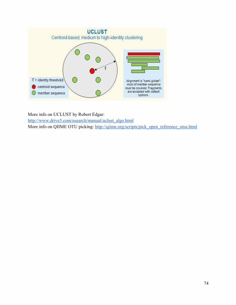
74
More info on UCLUST by Robert Edgar: http://www.drive5.com/usearch/manual/uclust_algo.html More info on QIIME OTU picking: http://qiime.org/scripts/pick_open_reference_otus.html

75
3.1_pick_otus.sh
1. Open 3.1_pick_otus.sh in the jc_qiime_pipeline folder. 2. Change the working directory to match where your input file is located.
What is the input file name?_________________________
What is the output file name?________________________
3. Save and submit the file to the Cluster. Check for the output file when the script is complete.
Initial analyses
Congratulations! You have successfully made an OTU table. Before we can jump into making sense of what bacteria are in our samples and why, we have to do some housekeeping to facilitate our downstream analysis. Our initial analysis includes 3 steps:
1. Getting the stats on the OTU table 2. Producing a rarified OTU table at an even sampling depth 3. Summarizing the rarified OTU table at various taxonomic levels
The scripts for these three steps can be found in the file 4_initial_analyses.md. All of these scripts are fairly simple, so you can copy and paste them into the command line, making modifications as necessary.
4_initial_analyses.md
Step 1: Getting stats on the OTU Table
Before analyzing the OTU table, it’s good idea to determine a cut-off point for the number of sequences/sample for downstream analysis. QIIME 1.8 employs the script biom summarize-table to report the stats of an OTU table, including the following:
1. Number of samples 2. Number of observations (OTUs) 3. Total number of sequences 4. Min/max number of sequences/sample 5. Mean and median sequences/sample 6. Standard deviation on sequences/sample 7. Number of sequences for each sample
Open 4_initial_analyses.md in the jc_qiime_pipeline folder. Modify the input/output file names. Then copy the example command into the terminal and run it. When it’s finished, open the resulting text file. (You can continue to use Cyberduck, or use less or nano in the terminal.)

76
Looking at the output file, answer the following:
How many samples are in the OTU table? ____________________
How many OTUs (observations) in the OTU table? _________________
Total number of sequences? _______________________
Min/max number of sequences? ______________________ The principal purpose of this script is to determine a good cut-off for the number of sequences in a sample in order for a sample to be included in downstream analysis. Looking at Counts/sample detail, what is a good sampling cut-off for our OTU table? When choosing an even sampling depth, it is important to maximize the number of samples kept while avoiding samples with a very low number of sequences. (Hint: a good rule of thumb is at least a few thousands sequences/sample.)
Sampling cut-off: ______________________ sequences/sample
How many samples does this cut-off exclude? _____________________

77
Step 2: Single rarefaction
As you saw in the output file above, the number of sequences per sample is highly variable. Currently, the accepted practice to account for varied sequence count is rarefication. Rarefaction is a standardization technique that subsamples all of your samples at the same depth. Samples below your rarefaction depth will be discarded while samples above will be resampled down to that number. As such, choosing a rarefaction depth is a balancing act between keeping samples and keeping sequences in those samples. We will set our rarefaction sampling depth at _____________, as determined above. The script requires the following arguments: -i input file path (.biom) -o outfile file path (.biom) -d depth, number of sequences to subsample per sample Again, open the file 4_initial_analyses.md, edit the rarefaction script, and run it through the terminal. It’s a good idea to include the sampling depth in the name of the output file, so you don’t confuse it with the original OTU table. The resulting OTU table should be used in all downstream analyses, except in alpha rarefaction and when using the beta diversity workflow. Step 3: Summarize Taxa The OTU table is divided into taxonomic level and either relative abundance or absolute abundance of each taxon in each sample is returned. These taxa summaries are useful to detect broad trends in the dataset and to make biplots (discussed in beta diversity section). There is a workflow script for generating summarized taxa plots; however we have found it easier to manipulate data in Excel. The default output of this script are taxa summaries in both tab delimited (.txt) and biom formats. Taxa are summarized by L2 = phylum, L3 = class, L4 = order, L5 = family, and L6 = genus. Taxa can also be summarized at the species level (L7); however the V4 region of the 16s rRNA gene typically does not provide enough resolution to get species level taxonomic information. summarize_taxa.py takes two arguments:
What is the input file name? _________________________
Is the output a file or a folder?________________________
Refer to http://qiime.org/scripts/summarize_taxa.html for additional informaiton.
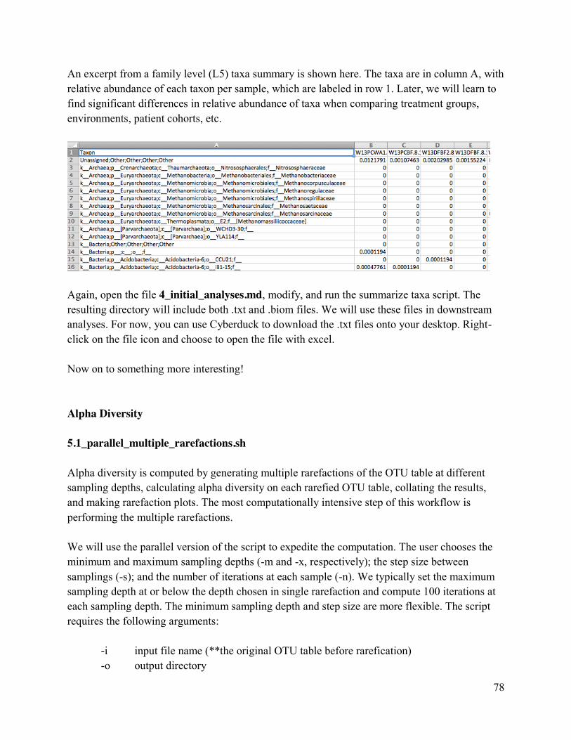
78
An excerpt from a family level (L5) taxa summary is shown here. The taxa are in column A, with relative abundance of each taxon per sample, which are labeled in row 1. Later, we will learn to find significant differences in relative abundance of taxa when comparing treatment groups, environments, patient cohorts, etc.
Again, open the file 4_initial_analyses.md, modify, and run the summarize taxa script. The resulting directory will include both .txt and .biom files. We will use these files in downstream analyses. For now, you can use Cyberduck to download the .txt files onto your desktop. Right-click on the file icon and choose to open the file with excel. Now on to something more interesting! Alpha Diversity 5.1_parallel_multiple_rarefactions.sh Alpha diversity is computed by generating multiple rarefactions of the OTU table at different sampling depths, calculating alpha diversity on each rarefied OTU table, collating the results, and making rarefaction plots. The most computationally intensive step of this workflow is performing the multiple rarefactions. We will use the parallel version of the script to expedite the computation. The user chooses the minimum and maximum sampling depths (-m and -x, respectively); the step size between samplings (-s); and the number of iterations at each sample (-n). We typically set the maximum sampling depth at or below the depth chosen in single rarefaction and compute 100 iterations at each sampling depth. The minimum sampling depth and step size are more flexible. The script requires the following arguments: -i input file name (**the original OTU table before rarefication) -o output directory

79
-m minimum sampling depth -x maximum sampling depth -s step size -n number of iterations Refer to http://qiime.org/scripts/multiple_rarefactions.html for additional information. Practice Exercise: Looking at the example below, answer the following questions. parallel_multiple_rarefactions.py -i otu_table_mc2_w_tax_no_pynast_failures.biom -o multiple_rars/ -O 30 -m 200 -n 100 -x 3200 -s 500 What is the minimum sampling depth? _________________ Max sampling depth? _________ Step size? ____________ Number of iterations? ________ How many rarified tables will this script yield in total? ____________________ Now, let’s think about producing multiple rarified tables from our OTU table. What could be our minimum sampling depth? _______________ Max sampling depth? _________ Step size? ____________ Number of iterations? ________ How many rarified tables will this script yield in total? ____________________ Edit 5.1_parallel_multiple_rarefactions.sh so it contains the directory name, input/output file names, and above parameters as necessary. Save and submit the file. Be prepared for the script to take some time to run. **Note: The script will likely hang (for reasons we have not yet pinned down). Use Cyberduck to check how many files are in the output folder. Once you have about 80 more files than you expect, cancel the job. The extra files are temporary files and will need to be deleted before moving on. After canceling the job, open the directory of rarified tables. Use rm -rf <insert directory name here> to delete the temporary directory, which will be listed as the last item. The next script is performed on the entire directory, and the presence of the temporary folder will cause the script to fail, as it is not a .biom file. The directory name will be a mix of numbers and letters.

80
5.2_parallel_alpha_diversity.sh We will now compute alpha diversity on the directory of rarified tables produced above. QIIME provides numerous alpha diversity metrics. The full list can be viewed by running the following script in the command line:
alpha_diversity.py -s Refer to http://qiime.org/scripts/parallel_alpha_diversity.html for additonal information. Open the files 5.2_parallel_alpha_diversity.sh. Which metrics are we using? ______________________________________________________________________________ ______________________________________________________________________________ Open and edit 5.2_alpha_diversity.sh to use the correct directories and methods. Save and submit the file. The script may appear to hang after a few minutes. After about 4 to 5 minutes, you may need to cancel the job using qdel <jobnumber>. **Note: Once the script finishes or you delete the job, open the alpha_div output directory. Use rm -rf <insert directory name here> to delete the temporary directory, which will be listed as the first item. The next script is performed on the entire directory of .txt files, and the presence of the temporary folder will cause the script to fail. Once again, the temporary directory name will be a mix of numbers and letters. 5.3_collate_and_plot.sh Finally, we collate the alpha diversity results at each sampling depth and plot the results as rarefaction curves. The output will provide us with an html file of the alpha rarefaction plots which can be viewed in a web browser. Below is an example of a rarefaction plot. The script requires a metadata file, which allows you to compare alpha diversity between sample groups, such as by treatment type or sampling location. The sampling depth is plotted on the x-axis, while the species richness or diversity (depending on which alpha diversity metric you used) is plotted on the y-axis.

81
Rarefaction plots can reveal differences in alpha diversity between treatments or time points. Here it seems that the alpha diversity in water samples is higher than the alpha diversity in biofilm samples. Since the error bars do not overlap, it looks like the difference is significant. We will confirm the statistical significance in the next section, using the script compare_alpha.py. Rarefaction plots can also tell you if the environment was sampled to an adequate depth. If the OTU richness increases as more OTUs are sampled, then you should probably rarefy to a deeper sampling depth. In this case, we observe species richness leveling off as sampling depth increases. This suggests that we have achieved adequate sequencing depth in our environmental samples. Refer to http://qiime.org/scripts/make_rarefaction_plots.html for more information about making rarefaction plots. Modify the directories inside 5.3_collate_and_plot.sh and submit the script. Once the script completes, use Cyberduck to copy the entire directory of rarefaction plots to your desktop. You may then open the enclosed HTML file. 5.4_compare_alpha_diversity.sh We can now determine if differences in alpha diversity are significant between sample groups using the script compare_alpha.py. You can chose both the metadata category to compare and

82
the alpha diversity metric. The script only works on categorical metadata parameters (such as sample location, treatment type, or patient cohort) or quantitative discrete data (such as sampling day). Further, you can use either a parametric or nonparametric two-sample t-test. Refer to http://qiime.org/scripts/compare_alpha_diversity.html for additional informaiton. Open 5.4_compare_alpha_diversity.sh and modify the metadata parameter (-c) and input file. You can run as many scripts in succession as you please. Save and submit the job to the Cluster. The output of this script is a tab delimited file containing pairwise alpha diversity comparisons. Copy the files to your desktop using Cyberduck and open in Excel for easier viewing. Below is an example of the output. Here, four groups from a different dataset were compared to yield six pairwise comparisons.
We can see the results of the nonparametric sample in columns A and B, along with respective means and standard deviations for each group. The t-test explains how the sample fits into the nonparametric distribution and the p-value indicates if the comparison is significant. Here, the difference in alpha diversity between the groups “NP” and “CC” is significant, as indicated by the p-value. Beta Diversity 6.1_beta_diversity_through_plots.sh QIIME offers a workflow script for computing beta diversity, although each step can be performed individually. The current workflow script produces 3D PCoA plots which can be visualized using Emperor. Emperor plots can be viewed in a web browser (i.e. Chrome). We will also use a second script to generate 2D plots which can be visualized as images in a web browser.

83
There are a number of different beta diversity metrics supported in QIIME. We have found the Unifrac distance metrics to be most useful and informative. Unifrac takes phylogenetic relatedness into account in computing beta diversity. Unweighted Unifrac regards only the presence or absence of taxa, whereas weighted Unifrac uses taxon relative abundance as well. Recently, there has been some debate over whether or not to rarefy an OTU table, as rarefying can affect the beta diversity results (depending on the metric). However, we have to decided to use an unrarified OTU table and accept only the weighted Unifrac results, disregarding the unweighted Unifrac results. Unweighted Unifrac results are only valid if calculated on a rarified table. See this paper for a more in-depth explanation: http://arxiv.org/abs/1310.0424 We will input the original OTU table. The script also requires a metadata file and a tree reference tree file available from Greengenes. We will use the 97_otus.tree file from the May 2013 release of Greengenes. Refer to http://qiime.org/scripts/beta_diversity_through_plots.html for additional information. Edit 6.1_beta_diversity_through_plots.sh so it contains the directory name, input/output file names, and above parameters as necessary. Save and submit the file. Once the job is complete, download the output directory to your desktop. Inside you will find several folders. Open the 2D folder to view the contents then open weighted_unifrac_pc_2D_PCoA_plots.html in a web browser. Hover over each point to see the sample ID and metadata value. An example of a 2D plot based on weighted Unifrac distances is shown below.
For the metadata parameter Sample_type, the points are colored by blue for water and red for biofilm. The first PCoA plot is of PC1 and PC2, or the two axes which explain the most variation

84
in the dataset. PC1 explains 45.19% and PC2 explains 43.12%. The next PCoA plot shows PC2 vs. PC3 and PC1 vs. PC3, respectively. We typically look at the first PCoA plot (PC1 vs. PC2) because the most variation in the dataset is explained by this ordination of samples based on their weighted Unifrac distances. Samples that are closer together have similar microbial communities than do samples that are farther apart. Notably, the sample orientation in space is random, so the direction of the gradient may flip if the plot is re-made. However, the trends and clustering are preserved. 3D Plots Now, let’s look at the 3D plots. In the beta diversity directory that you downloaded to your desktop, open the folder unweighted_unifrac_emporer_pcoa_plot and double-click on the index.html file. You will be redirected to Emperor in a modern browser (i.e. Chrome). Below is an example of a 3D plot.
You can also add taxonomy to your 3D plots in the form of biplots. While we are not demonstrating full use of that script here, you may enter make_emperor.py -h into the command line to view documentaiton of the script. Biplots are made by passing the -t flag along with a taxonomy-summarized OTU table in tab-delimited format (such as those created with summarize_taxa.py). Below is an example of a biplot at the phylum (L2) level.

85
*Important note about biplots: The type of OTU table used as input for beta diversity (calculation of the principal coordinate frame) must match the OTU table used as input for summarize taxa.py. For example, to create the biplot above, we used a single rarified OTU table as input for the beta diversity script. The same single rarified OTU table was used as input for the summarize taxa script. Multivariate Statistics QIIME offers a wealth of multivariate statistics to answer a range of questions about your dataset. Here we will demonstrate a few core analyses, including statistically comparing OTUs abundance between treatment groups, determining which metadata parameters best explain differences in community structure, and core microbiome computation. However, the QIIME developers routinely add additional analyses in software updates, so an astute researcher would benefit from checking the script documentation page frequently. Furthermore, OTU tables can be manipulated into data frames for analysis in R to produce heatmaps, Pearson correleations, etc. The possibilities are endless!
86
Compare Categories 7.1_compare_categories.sh Compare categories is a script used to determine which metadata parameters best describe differences in community structure (i.e. Unifrac distances). In this way, the script functions to describe how significant the clustering observed in PCoA plots is. The script provides various metrics to accommodate categorical, quantitative discrete, or quantitative continuous data. Several useful metrics are described below, but a complete list is available at http://qiime.org/scripts/compare_categories.html. adonis - Partitions a distance matrix among sources of variation in order to describe the strength and significance that a categorical or continuous variable has in determining variation of distances. This is a nonparametric method and is nearly equivalent to db-RDA (see below) except when distance matrices constructed with semi-metric or non-metric dissimilarities are provided, which may result in negative eigenvalues. adonis is very similar to PERMANOVA, though it is more robust in that it can accept either categorical or continuous variables in the metadata mapping file, while PERMANOVA can only accept categorical variables. See vegan::adonis for more details. ANOSIM - Tests whether two or more groups of samples are significantly different based on a categorical variable found in the metadata mapping file. You can specify a category in the metadata mapping file to separate samples into groups and then test whether there are significant differences between those groups. For example, you might test whether ‘Control’ samples are significantly different from ‘Fast’ samples. Since ANOSIM is nonparametric, significance is determined through permutations. See vegan::anosim for more details. PERMANOVA - This method is very similar to adonis except that it only accepts a categorical variable in the metadata mapping file. It uses an ANOVA experimental design and returns a pseudo-F value and a p-value. Since PERMANOVA is nonparametric, significance is determined through permutations. Are the metadata parameters “Sample_type” and “Source” categorical or quantitative? ______________________________________________________________________________ Which metric(s) can we use for these metadata parameters? _______________________________ ______________________________________________________________________________

87
In the examples provided, we use the anosim method to look at how the metadata parameters “Sample_type” and “Source” explain differences in community structure. Edit 7.1_compare_categories.sh and modify the metadata parameter (-c), directories, and input/output files as necessary. You can run as many scripts in succession as you please, changing out the metadata parameter of interests (-c) and the method. Save and submit the job to the Cluster. As output directory is made for each individual script run in the submission script. Use cd to look at the contents of an output directory. Inside, you’ll find a file called anosim_results.txt. Below is the result of the anosim metric on source.
The file reports the method used, the R statistic, the p-value, and the number of permutations. What is the R statistic? ____________________ P-value? _______________________________ The R statistic may be interpreted as the percent (out of 1) that a variable explains differences in community structure. With this in mind, “Source” describes _______________________ % of variation in community structure. Group Significance 7.2_group_significance.sh New to QIIME 1.8, the group_significance features non-parametric statistical tests. Importantly, OTU data is not normally distributed, so parametric stats are essentially irrelevant for our purposes. This script is one of the most robust ways to reveal key differences in OTU abundance between groups of samples. Unfortunately the documentation for this script is not available on the QIIME website; however, we can run group_significance.py -h directly in the command line to view the script documentation.

88
The particular test you want to use is designated by the -s flag. Available options are: nonparametric_t_test nonparametric comparison of two sample groups mann_whitney_u nonparametric comparison of two sample groups kruskal_wallis nonparametric comparison of two or more sample groups
(nonparametric ANVOVA) boostrap_mann_whitney_u bootstrap comparison of two sample groups g_test parametric comparison of two or more groups ANOVA parametric comparison of two or more sample groups parametric_t_test parametric comparison of two sample groups We generally use the mann_whitney_u test for comparison of two groups and the kruskall_walllis test for comparison of two or more groups. A rarified OTU table should be used as the input for this script. Notably, we can use either the single rarified table with OTUs down to the species level, or any of the taxa summarized OTU tables. The summarized tables are especially interesting for looking at OTU abundance differences at different taxonomic levels. If we want to compare sample type (water vs. biofilm), what would be an appropriate test to use? _____________________________________________________________________________ Which OTU table should we input to look at differences in OTU abundance at the phyla level? ______________________________________________________________________________ Practice Exercise: group_significance.py -i summarized_tax/otu_even_8375_L4.biom -m mini_meta.txt -s kruskal_wallis -c Source -o kruskal_wallis_source_L4 In the example above, what taxonomic level are we comparing? ___________________________ Based on the statistical test, are we comparing two or more than two groups of samples? ______________________________________________________________________________

89
Edit 7.2_group_signifiance and modify the directory, input/output files, and (-c) flags as you please. You can run many individual scripts in the submit file, as long as you carefully name the output files to reflect the statistical test performed and the OTU table used as input. The script outputs tab delimited files which you can download to your desktop and open in Excel. Below is an example from comparing samples by type (water or biofilm) at the family level.
In column A, we see OTUs summarized at the family level. The subsequent columns contain the test-statistic, p-value, FDR corrected p-value, and Bonferroni corrected p-value. Bonferroni is the most conservative method, while FDR (false discovery rate) is less conservative. Finally, the mean relative abundances of each group are found in the last two columns. These output files are especially useful for quickly creating plots and bar charts in Excel. For example, we could plot the relative abundance of all families that have Bonferroni-corrected p-values less than or equal to 0.05. We like to use conditional formatting in Excel to quickly highlight data of interest. Select the column E. Next, find the “Conditional formatting” icon in the formatting toolbar.
Under conditional formatting, select “Highlight cell rules.” Then select the operation you wish to perform, such as “Less than.” A window will appear, in which you apply the bounds of the rule. In our case, we will choose the operation “Less than or equal to” and enter 0.5. In this window you can also change the highlighting format (color of cell and text) as you see fit.

90
How many OTU families have Bonferroni p-values less than or equal to 0.05? _______________ While this is a simple example of how to use conditional formatting, you can apply conditional formatting in very creative ways. For example, conditional formatting can produce rough “heatmaps” of your data by applying color scales. Core Microbiome 7.3_compute_core_micobiome.sh Computation of the core microbiome is another way to compare differences in OTUs between sample groups. The default script produces core microbiomes at 50% to 100% with 5% increments. The script works in the following way: For an OTU to be considered part of the core at the 50% cut-off, it must be found in 50% of samples in a given group. For example, for an OTU to be considered part of the “biofilm” core, it must be found in 50% of all biofilm samples. For an OTU to be considered part of the core at the 100% cut-off, it must be found in 100% of samples of a given group. The researcher chooses what cut-off is most appropriate for his/her analysis. The core microbiome script can be modified to calculate the core microbiome outside of the 50% to 100% cut-off. A quick way to obtain presence/absence data across a sample group is to set the cut-off at 1% (--min_fraction for core 0.01). Edit the file 7.3_compute_core_microbiome.sh, and modify the directory, input/output file, and valid states as necessary. The script outputs tab delimited files which can be opened in Excel. Venn diagrams can be used to visually represent differences in core microbiomes. Below is a Venn diagram comparing OTU presence/absence data for a different dataset, organized into four sample groups. This figure was produced using Venny, available at: http://bioinfogp.cnb.csic.es/tools/venny/

91
Below are additional examples of figures created in Excel using files such as summarized taxa tables and group significance outputs. Get creative!

92
The group significance script was used to determine significantly different families between two treatment types. Families with Bonferroni corrected p-values less than or equal to 0.05 were are represented in this figure. Mean OTU family abundances of one group of samples (corn) were subtracting from the other (native prairie). Families that are more abundance in the native prairie treatment are right of the center axis while families more abundance in corn treatment are left of the center axis.

93
The data for this figure was produced by a previous version of the group significance script. All orders that made up less than 2% of both samples were filtered out so that the most abundant families were represented. The figure was made using the abundance graph option in Excel.

94
Assessments
In the Environmental Genomics folder on moodle and made available through (gcatseek.pbworks.com) this workshop you will find all of the bioinformatics and biostatistical worksheets, quizzes, activities, discussion questions, papers, and assessments. See weeks 6 through 14. Assessments questions are also embedded in the module 2 text, as well as the following questions:
Assessment for Module 2
1. Briefly describe each of the steps involved in analyzing high-throughput 16S rRNA gene sequencing datasets using the QIIME pipeline.
2. Describe what data one can find in an OTU table.
3. Compare and contrast alpha and beta diversity.
4. The plot below shows rarefaction curves for two samples green (top line) and blue (bottom line) for a measured alpha diversity metric (PD whole tree, a phylogenetic distance measure) Describe the purpose of performing rarefaction analyses and describe what the results below show about these two different samples.

95
5. The above plot is a Principal Coordinate Analysis based on a beta diversity metric from nine different samples. Describe the utility of these types of plots for microbial ecology research.

96
1. In the terminal what would you type to get to the ‘pg1’ directory. (Assume you start in home directory).
SampleID BarcodeSequence LinkerPrimerSequence PRIMER BARCODE
Day1.2143.A1
TCCTTAGAAGGC
GTGCCAGCMGCCGCGGTAA H09
806 rcbc 572
Day1.2143.A2
GATGGACTTCAA
GTGCCAGCMGCCGCGGTAA H10
806 rcbc 573
Day1.2143.B1
GGTACCTGCAAT
GTGCCAGCMGCCGCGGTAA F04
806 rcbc 543
Day1.2143.B2
TCGCCTATAAGG
GTGCCAGCMGCCGCGGTAA F05
806 rcbc 544
Day1.2143.C1
TCTAGCCTGGCA
GTGCCAGCMGCCGCGGTAA D11
806 rcbc 526
Day1.2143.C2
GCCGGTACTCTA
GTGCCAGCMGCCGCGGTAA E11
806 rcbc 538
Day2.0925.A1
CGAATGAGTCAT
GTGCCAGCMGCCGCGGTAA E01
806 rcbc 528
Day2.0925.A2
CGATATCAGTAG
GTGCCAGCMGCCGCGGTAA F01
806 rcbc 540
2. Identify the two problems with the above mapping file.
3. Explain in words what the following QIIME python script will do. Make sure you describe each of the parameters. add_qiime_labels.py -m mapping_file.txt -i file.fasta -n 1000000 -o labelled_seqs
4. Briefly describe how we quality filtered our sequences in QIIME and why its important to quality filter sequence data before performing data analysis.

97
5. Describe how you plan to assess microbial diversity in your study? What hypotheses do you have with respect to potential changes in diversity over the course of this study?
6. Give one advantage and one disadvantage of using a rarified OTU table to a specific sequencing depth.
7. Describe what the following QIIME script does. Please include a description of the –s and –c parameters. Also describe what the expected output would look like.
otu_category_significance.py -i rarefied_otu_tables -m Map.txt -s correlation -c pH -o correlation.txt
8. Why are divergence-based measures more robust than species based beta diversity measures?

98
9. Describe stepwise, how you would statistically compare alpha diversity metrics between communities?
Applications in the classroom
Weeks 6-14 of the Environmental Genomics Research Course address the following objectives:
Utilize a virtual machine to employ linux operating systems. Be able to understand directory structure, files and processes in linux Understand the overall workflow we will execute in QIIME. Describe the difference between alpha and beta diversity and how we use these metrics to
describe the microbial ecology of various ecosystems Understand how demultiplexing and quality filtering is achieved. Use ordination methods to compare microbial community data from different samples. Prepare metadata mapping files that are readable by QIIME. Describe the three ways OTU picking can be performed. Apply rarefaction analyses to normalize for sequencing depth. Describe methods of quantifying system change Describe sources of measurement error in biodiversity data and propose ways to deal
with these biases. Be able to describe and implement both quantitative and qualitative measures of alpha
and beta diversity Be able to implement QIIME scripts to measure alpha diversity in our samples and to
statistically compare these metrics across samples. Understand the pros and cons of using phylogenetic divergence as a measure of
biodiversity.
Time line of module
This module will be spread out during down times during lab activities during this 2.5 day workshop. However, in the environmental genomics research course I taught last semester we spread this out over weeks 6 through 14. Again this was my first time teaching the course so take things with a ‘grain of salt’.

99
Discussion Topics for class
The utility of Unix/Linux operating systems. How to develop independence to troubleshoot error messages Differences between alpha and beta diversity and which metric are appropriate for which
biological questions How to choose appropriate biostatistics for your biological question Limitations of currently available informatics and statistical methods.
References and Suggested Reading
Diversity
1. Lozupone CA, Knight R. 2008. Species divergence and the measurement of microbial
diversity. FEMS Microbiol. Rev. 32:557–578. 2. McMurdie PJ. Holmes S. Waste not, Want Not: Why Rarefying Microbiome Data is
Inadmissible. ArXiv e-prints 2013. http://arxiv.org/pdf/1310.0424v2.pdf 3. McMurdie PJ, Holmes S. Phyloseq: A bioconductor package for handling and analysis of
high-throughput phylogenetic sequence data. Pac Symp Biocomput. 2012: 2235-246. http://www.ncbi.nlm.nih.gov/pmc/articles/PMC3357092/
Clusstering Algorithms
2. Caporaso JG, Bittinger K, Bushman FD, DeSantis TZ, Andersen GL, Knight R. 2010. PyNAST: a flexible tool for aligning sequences to a template alignment. Bioinformatics 26:266–267.
3. Edgar RC. 2010. Search and clustering orders of magnitude faster than BLAST.
Bioinformatics 26:2460–2461. 4. Edgar RC. UPARSE: highly accurate OTU sequences from microbial amplicon reads.
Nature Methods. 10:996-998. http://www.nature.com/nmeth/journal/v10/n10/abs/nmeth.2604.html
QIIME Examples 5. Caporaso JG, et al. 2011. Moving pictures of the human microbiome. Genome Biol.
12:R50.
6. Kuczynski J, Stombaugh J, Walters WA, González A, Caporaso JG, Knight R. 2012.Using
100
QIIME to analyze 16S rRNA gene sequences from microbial communities. Curr Protoc Microbiol. Chapter 1:Unit 1E.5.. doi:10.1002/9780471729259.mc01e05s27.
7. QIIME allows analysis of high-throughput community sequencing data.Caporaso JG, Kuczynski J, Stombaugh J, Bittinger K, Bushman FD, Costello EK, Fierer N, Peña AG, Goodrich JK, Gordon JI, Huttley GA, Kelley ST, Knights D, Koenig JE, Ley RE, Lozupone CA, McDonald D, Muegge BD, Pirrung M, Reeder J, Sevinsky JR, Turnbaugh PJ, Walters WA, Widmann J, Yatsunenko T, Zaneveld J, Knight R. 2010.
Nat Methods. 7(5):335-6.
Other Useful Tools
QIIME forum. Search here for helpful answers to your questions. If you have searched the forum thoroughly and have not found helpful information then post your question. The Knight group will get back to you within a few hours. http://groups.google.com/group/qiime-forum
Pandaseq to QIIME http://squamules.blogspot.com/2013/02/pandaseq-to-qiime.html. (integrating paired end sequence data and getting it into QIIME).
Mothur is another 16S rRNA gene tool developed by Pat Schloss. http://www.mothur.org/
AXIOME is a new tool that integrates many different tools including QIIME. http://neufeld.github.io/AXIOME/
Lynch MD, Masella AP, Hall MW, Bartram AK, Neufeld JD. 2013. AXIOME: automated exploration of microbial diversity. Gigascience. doi: 10.1186/2047-217X-2-3.

101
Appendix A. Primers
16S
HHMI 2013 Primers
Well Name Sequence
A1 806rcbc192
CAAGCAGAAGACGGCATACGAGATGTCGAATTTGCGAGTCAGTCAGCCGGACTACHVGGGTWTCTAAT
A2 806rcbc193
CAAGCAGAAGACGGCATACGAGATGCATCAGAGTTAAGTCAGTCAGCCGGACTACHVGGGTWTCTAAT
A3 806rcbc194
CAAGCAGAAGACGGCATACGAGATGTGGTCATCGTAAGTCAGTCAGCCGGACTACHVGGGTWTCTAAT
A4 806rcbc195
CAAGCAGAAGACGGCATACGAGATCTGAAGGGCGAAAGTCAGTCAGCCGGACTACHVGGGTWTCTAAT
A5 806rcbc196
CAAGCAGAAGACGGCATACGAGATCGCTCACAGAATAGTCAGTCAGCCGGACTACHVGGGTWTCTAAT
A6 806rcbc197
CAAGCAGAAGACGGCATACGAGATATTCGGTAGTGCAGTCAGTCAGCCGGACTACHVGGGTWTCTAAT
A7 806rcbc198
CAAGCAGAAGACGGCATACGAGATCGAGCTGTTACCAGTCAGTCAGCCGGACTACHVGGGTWTCTAAT
A8 806rcbc199
CAAGCAGAAGACGGCATACGAGATCAACACATGCTGAGTCAGTCAGCCGGACTACHVGGGTWTCTAAT
A9 806rcbc200
CAAGCAGAAGACGGCATACGAGATATTCTCTCACGTAGTCAGTCAGCCGGACTACHVGGGTWTCTAAT
A10
806rcbc201
CAAGCAGAAGACGGCATACGAGATCGACTCTAAACGAGTCAGTCAGCCGGACTACHVGGGTWTCTAAT
A11
806rcbc202
CAAGCAGAAGACGGCATACGAGATGTCTTCAGCAAGAGTCAGTCAGCCGGACTACHVGGGTWTCTAAT
A12
806rcbc203
CAAGCAGAAGACGGCATACGAGATCGGATAACCTCCAGTCAGTCAGCCGGACTACHVGGGTWTCTAAT
B1 806rcbc204
CAAGCAGAAGACGGCATACGAGATAGGGTGACTTTAAGTCAGTCAGCCGGACTACHVGGGTWTCTAAT
B2 806rcbc205
CAAGCAGAAGACGGCATACGAGATGACTTCATGCGAAGTCAGTCAGCCGGACTACHVGGGTWTCTAAT
B3 806rcbc206
CAAGCAGAAGACGGCATACGAGATGCCTGTCTGCAAAGTCAGTCAGCCGGACTACHVGGGTWTCTAAT
B4 806rcbc207
CAAGCAGAAGACGGCATACGAGATACTGATGGCCTCAGTCAGTCAGCCGGACTACHVGGGTWTCTAAT
B5 806rcbc208
CAAGCAGAAGACGGCATACGAGATTTCGATGCCGCAAGTCAGTCAGCCGGACTACHVGGGTWTCTAAT
B6 806rcbc209
CAAGCAGAAGACGGCATACGAGATTGTGGCTCGTGTAGTCAGTCAGCCGGACTACHVGGGTWTCTAAT

102
B7 806rcbc210
CAAGCAGAAGACGGCATACGAGATAACTTTCAGGAGAGTCAGTCAGCCGGACTACHVGGGTWTCTAAT
B8 806rcbc211
CAAGCAGAAGACGGCATACGAGATTGCACGTGATAAAGTCAGTCAGCCGGACTACHVGGGTWTCTAAT
B9 806rcbc212
CAAGCAGAAGACGGCATACGAGATGTTCGGTGTCCAAGTCAGTCAGCCGGACTACHVGGGTWTCTAAT
B10
806rcbc213
CAAGCAGAAGACGGCATACGAGATAAGACAGCTATCAGTCAGTCAGCCGGACTACHVGGGTWTCTAAT
B11
806rcbc214
CAAGCAGAAGACGGCATACGAGATATTGACCGGTCAAGTCAGTCAGCCGGACTACHVGGGTWTCTAAT
B12
806rcbc215
CAAGCAGAAGACGGCATACGAGATTTCTCCATCACAAGTCAGTCAGCCGGACTACHVGGGTWTCTAAT
C1 806rcbc216
CAAGCAGAAGACGGCATACGAGATCGTAGGTAGAGGAGTCAGTCAGCCGGACTACHVGGGTWTCTAAT
C2 806rcbc217
CAAGCAGAAGACGGCATACGAGATATTTAGGACGACAGTCAGTCAGCCGGACTACHVGGGTWTCTAAT
C3 806rcbc218
CAAGCAGAAGACGGCATACGAGATGGATAGCCAAGGAGTCAGTCAGCCGGACTACHVGGGTWTCTAAT
C4 806rcbc219
CAAGCAGAAGACGGCATACGAGATTGGTTGGTTACGAGTCAGTCAGCCGGACTACHVGGGTWTCTAAT
C5 806rcbc220
CAAGCAGAAGACGGCATACGAGATGTCGTCCAAATGAGTCAGTCAGCCGGACTACHVGGGTWTCTAAT
C6 806rcbc221
CAAGCAGAAGACGGCATACGAGATCAACGTGCTCCAAGTCAGTCAGCCGGACTACHVGGGTWTCTAAT
C7 806rcbc222
CAAGCAGAAGACGGCATACGAGATTACACAAGTCGCAGTCAGTCAGCCGGACTACHVGGGTWTCTAAT
C8 806rcbc223
CAAGCAGAAGACGGCATACGAGATGCGTCCATGAATAGTCAGTCAGCCGGACTACHVGGGTWTCTAAT
C9 806rcbc224
CAAGCAGAAGACGGCATACGAGATGTAATGCGTAACAGTCAGTCAGCCGGACTACHVGGGTWTCTAAT
C10
806rcbc225
CAAGCAGAAGACGGCATACGAGATGTCGCCGTACATAGTCAGTCAGCCGGACTACHVGGGTWTCTAAT
C11
806rcbc226
CAAGCAGAAGACGGCATACGAGATGGAATCCGATTAAGTCAGTCAGCCGGACTACHVGGGTWTCTAAT
C12
806rcbc227
CAAGCAGAAGACGGCATACGAGATCACCCGATGGTTAGTCAGTCAGCCGGACTACHVGGGTWTCTAAT
D1 806rcbc228
CAAGCAGAAGACGGCATACGAGATTTCTGAGAGGTAAGTCAGTCAGCCGGACTACHVGGGTWTCTAAT
D2 806rcbc229
CAAGCAGAAGACGGCATACGAGATATCCCTACGGAAAGTCAGTCAGCCGGACTACHVGGGTWTCTAAT
D3 806rcbc230
CAAGCAGAAGACGGCATACGAGATGGTTCCATTAGGAGTCAGTCAGCCGGACTACHVGGGTWTCTAAT
D4 806rcbc231
CAAGCAGAAGACGGCATACGAGATGTGTTCCCAGAAAGTCAGTCAGCCGGACTACHVGGGTWTCTAAT
D5 806rcbc232
CAAGCAGAAGACGGCATACGAGATCCGAGGTATAATAGTCAGTCAGCCGGACTACHVGGGTWTCTAAT

103
D6 806rcbc233
CAAGCAGAAGACGGCATACGAGATAGCGTAATTAGCAGTCAGTCAGCCGGACTACHVGGGTWTCTAAT
D7 806rcbc234
CAAGCAGAAGACGGCATACGAGATCTCGTGAATGACAGTCAGTCAGCCGGACTACHVGGGTWTCTAAT
D8 806rcbc235
CAAGCAGAAGACGGCATACGAGATAGGTGAGTTCTAAGTCAGTCAGCCGGACTACHVGGGTWTCTAAT
D9 806rcbc236
CAAGCAGAAGACGGCATACGAGATCCTGTCCTATCTAGTCAGTCAGCCGGACTACHVGGGTWTCTAAT
D10
806rcbc237
CAAGCAGAAGACGGCATACGAGATGGTTTAACACGCAGTCAGTCAGCCGGACTACHVGGGTWTCTAAT
D11
806rcbc238
CAAGCAGAAGACGGCATACGAGATAGACAGTAGGAGAGTCAGTCAGCCGGACTACHVGGGTWTCTAAT
D12
806rcbc239
CAAGCAGAAGACGGCATACGAGATGCCACGACTTACAGTCAGTCAGCCGGACTACHVGGGTWTCTAAT
E1 806rcbc240
CAAGCAGAAGACGGCATACGAGATATTGTTCCTACCAGTCAGTCAGCCGGACTACHVGGGTWTCTAAT
E2 806rcbc241
CAAGCAGAAGACGGCATACGAGATGCCGTAAACTTGAGTCAGTCAGCCGGACTACHVGGGTWTCTAAT
E3 806rcbc242
CAAGCAGAAGACGGCATACGAGATGCAGATTTCCAGAGTCAGTCAGCCGGACTACHVGGGTWTCTAAT
E4 806rcbc243
CAAGCAGAAGACGGCATACGAGATAGATGATCAGTCAGTCAGTCAGCCGGACTACHVGGGTWTCTAAT
E5 806rcbc244
CAAGCAGAAGACGGCATACGAGATGAGACGTGTTCTAGTCAGTCAGCCGGACTACHVGGGTWTCTAAT
E6 806rcbc245
CAAGCAGAAGACGGCATACGAGATTATCACCGGCACAGTCAGTCAGCCGGACTACHVGGGTWTCTAAT
E7 806rcbc246
CAAGCAGAAGACGGCATACGAGATTATGCCAGAGATAGTCAGTCAGCCGGACTACHVGGGTWTCTAAT
E8 806rcbc247
CAAGCAGAAGACGGCATACGAGATAGGTCCAAATCAAGTCAGTCAGCCGGACTACHVGGGTWTCTAAT
E9 806rcbc248
CAAGCAGAAGACGGCATACGAGATACCGTGCTCACAAGTCAGTCAGCCGGACTACHVGGGTWTCTAAT
E10
806rcbc249
CAAGCAGAAGACGGCATACGAGATCTCCCTTTGTGTAGTCAGTCAGCCGGACTACHVGGGTWTCTAAT
E11
806rcbc250
CAAGCAGAAGACGGCATACGAGATAGCTGCACCTAAAGTCAGTCAGCCGGACTACHVGGGTWTCTAAT
E12
806rcbc251
CAAGCAGAAGACGGCATACGAGATCCTTGACCGATGAGTCAGTCAGCCGGACTACHVGGGTWTCTAAT
F1 806rcbc252
CAAGCAGAAGACGGCATACGAGATCTATCATCCTCAAGTCAGTCAGCCGGACTACHVGGGTWTCTAAT
F2 806rcbc253
CAAGCAGAAGACGGCATACGAGATACTCTAGCCGGTAGTCAGTCAGCCGGACTACHVGGGTWTCTAAT
F3 806rcbc254
CAAGCAGAAGACGGCATACGAGATCGATAGGCCTTAAGTCAGTCAGCCGGACTACHVGGGTWTCTAAT
F4 806rcbc255
CAAGCAGAAGACGGCATACGAGATAATGACCTCGTGAGTCAGTCAGCCGGACTACHVGGGTWTCTAAT

104
HHMI 2014 Primers
Well
Name Primer For PCR
A1 806rcbc0
CAAGCAGAAGACGGCATACGAGATTCCCTTGTCTCCAGTCAGTCAGCCGGACTACHVGGGTWTCTAAT
A2 806rcbc1
CAAGCAGAAGACGGCATACGAGATACGAGACTGATTAGTCAGTCAGCCGGACTACHVGGGTWTCTAAT
A3 806rcbc2
CAAGCAGAAGACGGCATACGAGATGCTGTACGGATTAGTCAGTCAGCCGGACTACHVGGGTWTCTAAT
A4 806rcbc3
CAAGCAGAAGACGGCATACGAGATATCACCAGGTGTAGTCAGTCAGCCGGACTACHVGGGTWTCTAAT
A5 806rcbc4
CAAGCAGAAGACGGCATACGAGATTGGTCAACGATAAGTCAGTCAGCCGGACTACHVGGGTWTCTAAT
A6 806rcbc5
CAAGCAGAAGACGGCATACGAGATATCGCACAGTAAAGTCAGTCAGCCGGACTACHVGGGTWTCTAAT
A7 806rcbc6
CAAGCAGAAGACGGCATACGAGATGTCGTGTAGCCTAGTCAGTCAGCCGGACTACHVGGGTWTCTAAT
A8 806rcbc7
CAAGCAGAAGACGGCATACGAGATAGCGGAGGTTAGAGTCAGTCAGCCGGACTACHVGGGTWTCTAAT
A9 806rcbc8
CAAGCAGAAGACGGCATACGAGATATCCTTTGGTTCAGTCAGTCAGCCGGACTACHVGGGTWTCTAAT
A10 806rcbc9
CAAGCAGAAGACGGCATACGAGATTACAGCGCATACAGTCAGTCAGCCGGACTACHVGGGTWTCTAAT
A11 806rcbc10
CAAGCAGAAGACGGCATACGAGATACCGGTATGTACAGTCAGTCAGCCGGACTACHVGGGTWTCTAAT
A12 806rcbc11
CAAGCAGAAGACGGCATACGAGATAATTGTGTCGGAAGTCAGTCAGCCGGACTACHVGGGTWTCTAAT

105
B1 806rcbc12
CAAGCAGAAGACGGCATACGAGATTGCATACACTGGAGTCAGTCAGCCGGACTACHVGGGTWTCTAAT
B2 806rcbc13
CAAGCAGAAGACGGCATACGAGATAGTCGAACGAGGAGTCAGTCAGCCGGACTACHVGGGTWTCTAAT
B3 806rcbc14
CAAGCAGAAGACGGCATACGAGATACCAGTGACTCAAGTCAGTCAGCCGGACTACHVGGGTWTCTAAT
B4 806rcbc15
CAAGCAGAAGACGGCATACGAGATGAATACCAAGTCAGTCAGTCAGCCGGACTACHVGGGTWTCTAAT
B5 806rcbc16
CAAGCAGAAGACGGCATACGAGATGTAGATCGTGTAAGTCAGTCAGCCGGACTACHVGGGTWTCTAAT
B6 806rcbc17
CAAGCAGAAGACGGCATACGAGATTAACGTGTGTGCAGTCAGTCAGCCGGACTACHVGGGTWTCTAAT
B7 806rcbc18
CAAGCAGAAGACGGCATACGAGATCATTATGGCGTGAGTCAGTCAGCCGGACTACHVGGGTWTCTAAT
B8 806rcbc19
CAAGCAGAAGACGGCATACGAGATCCAATACGCCTGAGTCAGTCAGCCGGACTACHVGGGTWTCTAAT
B9 806rcbc20
CAAGCAGAAGACGGCATACGAGATGATCTGCGATCCAGTCAGTCAGCCGGACTACHVGGGTWTCTAAT
B10 806rcbc21
CAAGCAGAAGACGGCATACGAGATCAGCTCATCAGCAGTCAGTCAGCCGGACTACHVGGGTWTCTAAT
B11 806rcbc22
CAAGCAGAAGACGGCATACGAGATCAAACAACAGCTAGTCAGTCAGCCGGACTACHVGGGTWTCTAAT
B12 806rcbc23
CAAGCAGAAGACGGCATACGAGATGCAACACCATCCAGTCAGTCAGCCGGACTACHVGGGTWTCTAAT
C1 806rcbc24
CAAGCAGAAGACGGCATACGAGATGCGATATATCGCAGTCAGTCAGCCGGACTACHVGGGTWTCTAAT
C2 806rcbc25
CAAGCAGAAGACGGCATACGAGATCGAGCAATCCTAAGTCAGTCAGCCGGACTACHVGGGTWTCTAAT
C3 806rcbc26
CAAGCAGAAGACGGCATACGAGATAGTCGTGCACATAGTCAGTCAGCCGGACTACHVGGGTWTCTAAT

106
C4 806rcbc27
CAAGCAGAAGACGGCATACGAGATGTATCTGCGCGTAGTCAGTCAGCCGGACTACHVGGGTWTCTAAT
C5 806rcbc28
CAAGCAGAAGACGGCATACGAGATCGAGGGAAAGTCAGTCAGTCAGCCGGACTACHVGGGTWTCTAAT
C6 806rcbc29
CAAGCAGAAGACGGCATACGAGATCAAATTCGGGATAGTCAGTCAGCCGGACTACHVGGGTWTCTAAT
C7 806rcbc30
CAAGCAGAAGACGGCATACGAGATAGATTGACCAACAGTCAGTCAGCCGGACTACHVGGGTWTCTAAT
C8 806rcbc31
CAAGCAGAAGACGGCATACGAGATAGTTACGAGCTAAGTCAGTCAGCCGGACTACHVGGGTWTCTAAT
C9 806rcbc32
CAAGCAGAAGACGGCATACGAGATGCATATGCACTGAGTCAGTCAGCCGGACTACHVGGGTWTCTAAT
C10 806rcbc33
CAAGCAGAAGACGGCATACGAGATCAACTCCCGTGAAGTCAGTCAGCCGGACTACHVGGGTWTCTAAT
C11 806rcbc34
CAAGCAGAAGACGGCATACGAGATTTGCGTTAGCAGAGTCAGTCAGCCGGACTACHVGGGTWTCTAAT
C12 806rcbc35
CAAGCAGAAGACGGCATACGAGATTACGAGCCCTAAAGTCAGTCAGCCGGACTACHVGGGTWTCTAAT
D1 806rcbc36
CAAGCAGAAGACGGCATACGAGATCACTACGCTAGAAGTCAGTCAGCCGGACTACHVGGGTWTCTAAT
D2 806rcbc37
CAAGCAGAAGACGGCATACGAGATTGCAGTCCTCGAAGTCAGTCAGCCGGACTACHVGGGTWTCTAAT
D3 806rcbc38
CAAGCAGAAGACGGCATACGAGATACCATAGCTCCGAGTCAGTCAGCCGGACTACHVGGGTWTCTAAT
D4 806rcbc39
CAAGCAGAAGACGGCATACGAGATTCGACATCTCTTAGTCAGTCAGCCGGACTACHVGGGTWTCTAAT
D5 806rcbc40
CAAGCAGAAGACGGCATACGAGATGAACACTTTGGAAGTCAGTCAGCCGGACTACHVGGGTWTCTAAT
D6 806rcbc41
CAAGCAGAAGACGGCATACGAGATGAGCCATCTGTAAGTCAGTCAGCCGGACTACHVGGGTWTCTAAT

107
D7 806rcbc42
CAAGCAGAAGACGGCATACGAGATTTGGGTACACGTAGTCAGTCAGCCGGACTACHVGGGTWTCTAAT
D8 806rcbc43
CAAGCAGAAGACGGCATACGAGATAAGGCGCTCCTTAGTCAGTCAGCCGGACTACHVGGGTWTCTAAT
D9 806rcbc44
CAAGCAGAAGACGGCATACGAGATTAATACGGATCGAGTCAGTCAGCCGGACTACHVGGGTWTCTAAT
D10 806rcbc45
CAAGCAGAAGACGGCATACGAGATTCGGAATTAGACAGTCAGTCAGCCGGACTACHVGGGTWTCTAAT
D11 806rcbc46
CAAGCAGAAGACGGCATACGAGATTGTGAATTCGGAAGTCAGTCAGCCGGACTACHVGGGTWTCTAAT
D12 806rcbc47
CAAGCAGAAGACGGCATACGAGATCATTCGTGGCGTAGTCAGTCAGCCGGACTACHVGGGTWTCTAAT
E1 806rcbc48
CAAGCAGAAGACGGCATACGAGATTACTACGTGGCCAGTCAGTCAGCCGGACTACHVGGGTWTCTAAT
E2 806rcbc49
CAAGCAGAAGACGGCATACGAGATGGCCAGTTCCTAAGTCAGTCAGCCGGACTACHVGGGTWTCTAAT
E3 806rcbc50
CAAGCAGAAGACGGCATACGAGATGATGTTCGCTAGAGTCAGTCAGCCGGACTACHVGGGTWTCTAAT
E4 806rcbc51
CAAGCAGAAGACGGCATACGAGATCTATCTCCTGTCAGTCAGTCAGCCGGACTACHVGGGTWTCTAAT
E5 806rcbc52
CAAGCAGAAGACGGCATACGAGATACTCACAGGAATAGTCAGTCAGCCGGACTACHVGGGTWTCTAAT
E6 806rcbc53
CAAGCAGAAGACGGCATACGAGATATGATGAGCCTCAGTCAGTCAGCCGGACTACHVGGGTWTCTAAT
E7 806rcbc54
CAAGCAGAAGACGGCATACGAGATGTCGACAGAGGAAGTCAGTCAGCCGGACTACHVGGGTWTCTAAT
E8 806rcbc55
CAAGCAGAAGACGGCATACGAGATTGTCGCAAATAGAGTCAGTCAGCCGGACTACHVGGGTWTCTAAT
E9 806rcbc56
CAAGCAGAAGACGGCATACGAGATCATCCCTCTACTAGTCAGTCAGCCGGACTACHVGGGTWTCTAAT

108
E10 806rcbc57
CAAGCAGAAGACGGCATACGAGATTATACCGCTGCGAGTCAGTCAGCCGGACTACHVGGGTWTCTAAT
E11 806rcbc58
CAAGCAGAAGACGGCATACGAGATAGTTGAGGCATTAGTCAGTCAGCCGGACTACHVGGGTWTCTAAT
E12 806rcbc59
CAAGCAGAAGACGGCATACGAGATACAATAGACACCAGTCAGTCAGCCGGACTACHVGGGTWTCTAAT
F1 806rcbc60
CAAGCAGAAGACGGCATACGAGATCGGTCAATTGACAGTCAGTCAGCCGGACTACHVGGGTWTCTAAT
F2 806rcbc61
CAAGCAGAAGACGGCATACGAGATGTGGAGTCTCATAGTCAGTCAGCCGGACTACHVGGGTWTCTAAT
F3 806rcbc62
CAAGCAGAAGACGGCATACGAGATGCTCGAAGATTCAGTCAGTCAGCCGGACTACHVGGGTWTCTAAT
F4 806rcbc63
CAAGCAGAAGACGGCATACGAGATAGGCTTACGTGTAGTCAGTCAGCCGGACTACHVGGGTWTCTAAT
Fungal ITS
Well Name Sequence
A1 ITS2rcbc0
CAAGCAGAAGACGGCATACGAGATTCCCTTGTCTCCAGTCAGTCAGATGCTGCGTTCTTCATCGATGC
A2 ITS2rcbc1
CAAGCAGAAGACGGCATACGAGATACGAGACTGATTAGTCAGTCAGATGCTGCGTTCTTCATCGATGC
A3 ITS2rcbc2
CAAGCAGAAGACGGCATACGAGATGCTGTACGGATTAGTCAGTCAGATGCTGCGTTCTTCATCGATGC
A4 ITS2rcbc3
CAAGCAGAAGACGGCATACGAGATATCACCAGGTGTAGTCAGTCAGATGCTGCGTTCTTCATCGATGC
A5 ITS2rcbc4
CAAGCAGAAGACGGCATACGAGATTGGTCAACGATAAGTCAGTCAGATGCTGCGTTCTTCATCGATGC
A6 ITS2rcbc5
CAAGCAGAAGACGGCATACGAGATATCGCACAGTAAAGTCAGTCAGATGCTGCGTTCTTCATCGATGC
A7 ITS2rcbc6
CAAGCAGAAGACGGCATACGAGATGTCGTGTAGCCTAGTCAGTCAGATGCTGCGTTCTTCATCGATGC
A8 ITS2rcbc7
CAAGCAGAAGACGGCATACGAGATAGCGGAGGTTAGAGTCAGTCAGATGCTGCGTTCTTCATCGATGC
A9 ITS2rcbc8
CAAGCAGAAGACGGCATACGAGATATCCTTTGGTTCAGTCAGTCAGATGCTGCGTTCTTCATCGATGC
A1 ITS2rc CAAGCAGAAGACGGCATACGAGATTACAGCGCATACAGTCAGTCA

109
0 bc9 GATGCTGCGTTCTTCATCGATGC A11
ITS2rcbc10
CAAGCAGAAGACGGCATACGAGATACCGGTATGTACAGTCAGTCAGATGCTGCGTTCTTCATCGATGC
A12
ITS2rcbc11
CAAGCAGAAGACGGCATACGAGATAATTGTGTCGGAAGTCAGTCAGATGCTGCGTTCTTCATCGATGC
B1 ITS2rcbc12
CAAGCAGAAGACGGCATACGAGATTGCATACACTGGAGTCAGTCAGATGCTGCGTTCTTCATCGATGC
B2 ITS2rcbc13
CAAGCAGAAGACGGCATACGAGATAGTCGAACGAGGAGTCAGTCAGATGCTGCGTTCTTCATCGATGC
B3 ITS2rcbc14
CAAGCAGAAGACGGCATACGAGATACCAGTGACTCAAGTCAGTCAGATGCTGCGTTCTTCATCGATGC
B4 ITS2rcbc15
CAAGCAGAAGACGGCATACGAGATGAATACCAAGTCAGTCAGTCAGATGCTGCGTTCTTCATCGATGC
B5 ITS2rcbc16
CAAGCAGAAGACGGCATACGAGATGTAGATCGTGTAAGTCAGTCAGATGCTGCGTTCTTCATCGATGC
B6 ITS2rcbc17
CAAGCAGAAGACGGCATACGAGATTAACGTGTGTGCAGTCAGTCAGATGCTGCGTTCTTCATCGATGC
B7 ITS2rcbc18
CAAGCAGAAGACGGCATACGAGATCATTATGGCGTGAGTCAGTCAGATGCTGCGTTCTTCATCGATGC
B8 ITS2rcbc19
CAAGCAGAAGACGGCATACGAGATCCAATACGCCTGAGTCAGTCAGATGCTGCGTTCTTCATCGATGC
B9 ITS2rcbc20
CAAGCAGAAGACGGCATACGAGATGATCTGCGATCCAGTCAGTCAGATGCTGCGTTCTTCATCGATGC
B10
ITS2rcbc21
CAAGCAGAAGACGGCATACGAGATCAGCTCATCAGCAGTCAGTCAGATGCTGCGTTCTTCATCGATGC
B11
ITS2rcbc22
CAAGCAGAAGACGGCATACGAGATCAAACAACAGCTAGTCAGTCAGATGCTGCGTTCTTCATCGATGC
B12
ITS2rcbc23
CAAGCAGAAGACGGCATACGAGATGCAACACCATCCAGTCAGTCAGATGCTGCGTTCTTCATCGATGC
C1 ITS2rcbc24
CAAGCAGAAGACGGCATACGAGATGCGATATATCGCAGTCAGTCAGATGCTGCGTTCTTCATCGATGC
C2 ITS2rcbc25
CAAGCAGAAGACGGCATACGAGATCGAGCAATCCTAAGTCAGTCAGATGCTGCGTTCTTCATCGATGC
C3 ITS2rcbc26
CAAGCAGAAGACGGCATACGAGATAGTCGTGCACATAGTCAGTCAGATGCTGCGTTCTTCATCGATGC
C4 ITS2rcbc27
CAAGCAGAAGACGGCATACGAGATGTATCTGCGCGTAGTCAGTCAGATGCTGCGTTCTTCATCGATGC
C5 ITS2rcbc28
CAAGCAGAAGACGGCATACGAGATCGAGGGAAAGTCAGTCAGTCAGATGCTGCGTTCTTCATCGATGC
C6 ITS2rcbc29
CAAGCAGAAGACGGCATACGAGATCAAATTCGGGATAGTCAGTCAGATGCTGCGTTCTTCATCGATGC
C7 ITS2rcbc30
CAAGCAGAAGACGGCATACGAGATAGATTGACCAACAGTCAGTCAGATGCTGCGTTCTTCATCGATGC
C8 ITS2rcbc31
CAAGCAGAAGACGGCATACGAGATAGTTACGAGCTAAGTCAGTCAGATGCTGCGTTCTTCATCGATGC

110
C9 ITS2rcbc32
CAAGCAGAAGACGGCATACGAGATGCATATGCACTGAGTCAGTCAGATGCTGCGTTCTTCATCGATGC
C10
ITS2rcbc33
CAAGCAGAAGACGGCATACGAGATCAACTCCCGTGAAGTCAGTCAGATGCTGCGTTCTTCATCGATGC
C11
ITS2rcbc34
CAAGCAGAAGACGGCATACGAGATTTGCGTTAGCAGAGTCAGTCAGATGCTGCGTTCTTCATCGATGC
C12
ITS2rcbc35
CAAGCAGAAGACGGCATACGAGATTACGAGCCCTAAAGTCAGTCAGATGCTGCGTTCTTCATCGATGC
D1 ITS2rcbc36
CAAGCAGAAGACGGCATACGAGATCACTACGCTAGAAGTCAGTCAGATGCTGCGTTCTTCATCGATGC
D2 ITS2rcbc37
CAAGCAGAAGACGGCATACGAGATTGCAGTCCTCGAAGTCAGTCAGATGCTGCGTTCTTCATCGATGC
D3 ITS2rcbc38
CAAGCAGAAGACGGCATACGAGATACCATAGCTCCGAGTCAGTCAGATGCTGCGTTCTTCATCGATGC
D4 ITS2rcbc39
CAAGCAGAAGACGGCATACGAGATTCGACATCTCTTAGTCAGTCAGATGCTGCGTTCTTCATCGATGC
D5 ITS2rcbc40
CAAGCAGAAGACGGCATACGAGATGAACACTTTGGAAGTCAGTCAGATGCTGCGTTCTTCATCGATGC
D6 ITS2rcbc41
CAAGCAGAAGACGGCATACGAGATGAGCCATCTGTAAGTCAGTCAGATGCTGCGTTCTTCATCGATGC
D7 ITS2rcbc42
CAAGCAGAAGACGGCATACGAGATTTGGGTACACGTAGTCAGTCAGATGCTGCGTTCTTCATCGATGC
D8 ITS2rcbc43
CAAGCAGAAGACGGCATACGAGATAAGGCGCTCCTTAGTCAGTCAGATGCTGCGTTCTTCATCGATGC
D9 ITS2rcbc44
CAAGCAGAAGACGGCATACGAGATTAATACGGATCGAGTCAGTCAGATGCTGCGTTCTTCATCGATGC
D10
ITS2rcbc45
CAAGCAGAAGACGGCATACGAGATTCGGAATTAGACAGTCAGTCAGATGCTGCGTTCTTCATCGATGC
D11
ITS2rcbc46
CAAGCAGAAGACGGCATACGAGATTGTGAATTCGGAAGTCAGTCAGATGCTGCGTTCTTCATCGATGC
D12
ITS2rcbc47
CAAGCAGAAGACGGCATACGAGATCATTCGTGGCGTAGTCAGTCAGATGCTGCGTTCTTCATCGATGC
E1 ITS2rcbc48
CAAGCAGAAGACGGCATACGAGATTACTACGTGGCCAGTCAGTCAGATGCTGCGTTCTTCATCGATGC
E2 ITS2rcbc49
CAAGCAGAAGACGGCATACGAGATGGCCAGTTCCTAAGTCAGTCAGATGCTGCGTTCTTCATCGATGC
E3 ITS2rcbc50
CAAGCAGAAGACGGCATACGAGATGATGTTCGCTAGAGTCAGTCAGATGCTGCGTTCTTCATCGATGC
E4 ITS2rcbc51
CAAGCAGAAGACGGCATACGAGATCTATCTCCTGTCAGTCAGTCAGATGCTGCGTTCTTCATCGATGC
E5 ITS2rcbc52
CAAGCAGAAGACGGCATACGAGATACTCACAGGAATAGTCAGTCAGATGCTGCGTTCTTCATCGATGC
E6 ITS2rcbc53
CAAGCAGAAGACGGCATACGAGATATGATGAGCCTCAGTCAGTCAGATGCTGCGTTCTTCATCGATGC
E7 ITS2rcbc54
CAAGCAGAAGACGGCATACGAGATGTCGACAGAGGAAGTCAGTCAGATGCTGCGTTCTTCATCGATGC

111
E8 ITS2rcbc55
CAAGCAGAAGACGGCATACGAGATTGTCGCAAATAGAGTCAGTCAGATGCTGCGTTCTTCATCGATGC
E9 ITS2rcbc56
CAAGCAGAAGACGGCATACGAGATCATCCCTCTACTAGTCAGTCAGATGCTGCGTTCTTCATCGATGC
E10
ITS2rcbc57
CAAGCAGAAGACGGCATACGAGATTATACCGCTGCGAGTCAGTCAGATGCTGCGTTCTTCATCGATGC
E11
ITS2rcbc58
CAAGCAGAAGACGGCATACGAGATAGTTGAGGCATTAGTCAGTCAGATGCTGCGTTCTTCATCGATGC
E12
ITS2rcbc59
CAAGCAGAAGACGGCATACGAGATACAATAGACACCAGTCAGTCAGATGCTGCGTTCTTCATCGATGC
F1 ITS2rcbc60
CAAGCAGAAGACGGCATACGAGATCGGTCAATTGACAGTCAGTCAGATGCTGCGTTCTTCATCGATGC
F2 ITS2rcbc61
CAAGCAGAAGACGGCATACGAGATGTGGAGTCTCATAGTCAGTCAGATGCTGCGTTCTTCATCGATGC
F3 ITS2rcbc62
CAAGCAGAAGACGGCATACGAGATGCTCGAAGATTCAGTCAGTCAGATGCTGCGTTCTTCATCGATGC
F4 ITS2rcbc63
CAAGCAGAAGACGGCATACGAGATAGGCTTACGTGTAGTCAGTCAGATGCTGCGTTCTTCATCGATGC
F5 ITS2rcbc64
CAAGCAGAAGACGGCATACGAGATTCTCTACCACTCAGTCAGTCAGATGCTGCGTTCTTCATCGATGC
F6 ITS2rcbc65
CAAGCAGAAGACGGCATACGAGATACTTCCAACTTCAGTCAGTCAGATGCTGCGTTCTTCATCGATGC
F7 ITS2rcbc66
CAAGCAGAAGACGGCATACGAGATCTCACCTAGGAAAGTCAGTCAGATGCTGCGTTCTTCATCGATGC
F8 ITS2rcbc67
CAAGCAGAAGACGGCATACGAGATGTGTTGTCGTGCAGTCAGTCAGATGCTGCGTTCTTCATCGATGC
F9 ITS2rcbc68
CAAGCAGAAGACGGCATACGAGATCCACAGATCGATAGTCAGTCAGATGCTGCGTTCTTCATCGATGC
F10
ITS2rcbc69
CAAGCAGAAGACGGCATACGAGATTATCGACACAAGAGTCAGTCAGATGCTGCGTTCTTCATCGATGC
F11
ITS2rcbc70
CAAGCAGAAGACGGCATACGAGATGATTCCGGCTCAAGTCAGTCAGATGCTGCGTTCTTCATCGATGC
F12
ITS2rcbc71
CAAGCAGAAGACGGCATACGAGATCGTAATTGCCGCAGTCAGTCAGATGCTGCGTTCTTCATCGATGC
G1 ITS2rcbc72
CAAGCAGAAGACGGCATACGAGATGGTGACTAGTTCAGTCAGTCAGATGCTGCGTTCTTCATCGATGC
G2 ITS2rcbc73
CAAGCAGAAGACGGCATACGAGATATGGGTTCCGTCAGTCAGTCAGATGCTGCGTTCTTCATCGATGC
G3 ITS2rcbc74
CAAGCAGAAGACGGCATACGAGATTAGGCATGCTTGAGTCAGTCAGATGCTGCGTTCTTCATCGATGC
G4 ITS2rcbc75
CAAGCAGAAGACGGCATACGAGATAACTAGTTCAGGAGTCAGTCAGATGCTGCGTTCTTCATCGATGC
G5 ITS2rcbc76
CAAGCAGAAGACGGCATACGAGATATTCTGCCGAAGAGTCAGTCAGATGCTGCGTTCTTCATCGATGC
G6 ITS2rcbc77
CAAGCAGAAGACGGCATACGAGATAGCATGTCCCGTAGTCAGTCAGATGCTGCGTTCTTCATCGATGC

112
G7 ITS2rcbc78
CAAGCAGAAGACGGCATACGAGATGTACGATATGACAGTCAGTCAGATGCTGCGTTCTTCATCGATGC
G8 ITS2rcbc79
CAAGCAGAAGACGGCATACGAGATGTGGTGGTTTCCAGTCAGTCAGATGCTGCGTTCTTCATCGATGC
G9 ITS2rcbc80
CAAGCAGAAGACGGCATACGAGATTAGTATGCGCAAAGTCAGTCAGATGCTGCGTTCTTCATCGATGC
G10
ITS2rcbc81
CAAGCAGAAGACGGCATACGAGATTGCGCTGAATGTAGTCAGTCAGATGCTGCGTTCTTCATCGATGC
G11
ITS2rcbc82
CAAGCAGAAGACGGCATACGAGATATGGCTGTCAGTAGTCAGTCAGATGCTGCGTTCTTCATCGATGC
G12
ITS2rcbc83
CAAGCAGAAGACGGCATACGAGATGTTCTCTTCTCGAGTCAGTCAGATGCTGCGTTCTTCATCGATGC
H1 ITS2rcbc84
CAAGCAGAAGACGGCATACGAGATCGTAAGATGCCTAGTCAGTCAGATGCTGCGTTCTTCATCGATGC
H2 ITS2rcbc85
CAAGCAGAAGACGGCATACGAGATGCGTTCTAGCTGAGTCAGTCAGATGCTGCGTTCTTCATCGATGC
H3 ITS2rcbc86
CAAGCAGAAGACGGCATACGAGATGTTGTTCTGGGAAGTCAGTCAGATGCTGCGTTCTTCATCGATGC
H4 ITS2rcbc87
CAAGCAGAAGACGGCATACGAGATGGACTTCCAGCTAGTCAGTCAGATGCTGCGTTCTTCATCGATGC
H5 ITS2rcbc88
CAAGCAGAAGACGGCATACGAGATCTCACAACCGTGAGTCAGTCAGATGCTGCGTTCTTCATCGATGC
H6 ITS2rcbc89
CAAGCAGAAGACGGCATACGAGATCTGCTATTCCTCAGTCAGTCAGATGCTGCGTTCTTCATCGATGC
H7 ITS2rcbc90
CAAGCAGAAGACGGCATACGAGATATGTCACCGCTGAGTCAGTCAGATGCTGCGTTCTTCATCGATGC
H8 ITS2rcbc91
CAAGCAGAAGACGGCATACGAGATTGTAACGCCGATAGTCAGTCAGATGCTGCGTTCTTCATCGATGC
H9 ITS2rcbc92
CAAGCAGAAGACGGCATACGAGATAGCAGAACATCTAGTCAGTCAGATGCTGCGTTCTTCATCGATGC
H10
ITS2rcbc93
CAAGCAGAAGACGGCATACGAGATTGGAGTAGGTGGAGTCAGTCAGATGCTGCGTTCTTCATCGATGC
H11
ITS2rcbc94
CAAGCAGAAGACGGCATACGAGATTTGGCTCTATTCAGTCAGTCAGATGCTGCGTTCTTCATCGATGC
H12
ITS2rcbc95
CAAGCAGAAGACGGCATACGAGATGATCCCACGTACAGTCAGTCAGATGCTGCGTTCTTCATCGATGC
B. Helpful Links
QIIME links
1. Main website http://qiime.org/index.html

113
2. Documentation http://qiime.org/documentation/index.html
3. Scripts http://qiime.org/scripts/index.html
4. More extensive information, news, and code can be found at QIIME’s github site.
https://github.com/qiime/qiime
Greengenes
http://greengenes.lbl.gov/cgi-bin/nph-index.cgi
Biom Format Documentation (OTU tables)
http://biom-format.org/
Linux for Beginners
http://www.linux.org/tutorial/view/beginners-level-course
Collection of File Management Commands
http://www.tuxfiles.org/linuxhelp/files.html
C. Additional Protocols/Scripts
1. ITS Region Amplification and Tools
PCR amplification
2. ITS Illumina tag PCR The ITS1-F and ITS2 primer pair2 with appropriate Illumina adapters, pad and linker sequences, and 12 bp Golay barcodes is used to amplify the ITS-1 region (Gardes & Bruns, 1993). The PCR conditions are based on the Earth Microbiome Project standard amplification protocols and have been used in recent papers (McGuire et al, 2013). PCR reactions will be performed in duplicate.

114
ITS1-F CTTGGTCATTTAGAGGAAGTAA ITS2 GCTGCGTTCTTCATCGATGC Record the PCR plate set up in the appropriate spreadsheet on the flash drive. Table 3. Components of the PCR reaction for ITS-1 amplification.
Reagent [Initial]
Volume
[Final] Num. Rxns
Amount
HotStarTaq Plus MM kit 2X 12.5 1X
DNA template 1.0
Forward Primer 5 μM 1.0 0.2 μM
Reverse primer 5 μM 1.0 0.2 μM
PCR grade H2O 9.5
Reaction volume 25.0
The master mix provided contains the HotStarTaq MM (buffer, dNTPs, and Taq), forward primer, and PCR grade H2O. Add 23 μl of the provided master mix, 1.0 μl reverse primer, and 1.0 μl template into each well.
When making negative controls, use 1.0 μl PCR grade H2O instead of the template. Between 5% and 10% of the samples should be negative controls if space permits.
When setting up your own reactions, use the last two columns to determine how much of each component you will need given the total number of samples and negative controls. Then aliquot 23 μl of this master mix into each well and add the unique components afterward.
Thermocycling Conditions
1. 94°C for 3 min to denature the DNA 2. 94 °C for 45 s 3. 50 °C for 60 s 4. 72 °C for 90 s 5. 72 °C for 10 min for final extension 6. 4 °C HOLD
Expected amplification size
ITS amplification products have a wider ranges usually 300-500 bp

115
b. QIIME Fungal ITS Workflow
Obtain Tutorial Files
The QIIME documentation contains example files you can use to practice the workflow. The tutorial files are from a study of the fungal community in soils Use wget to download the files and the ITS reference OTUs.
Download tutorial files and reference OTUs
Type wget https://s3.amazonaws.com/s3-qiime_tutorial_files/its-soils-tutorial.tgz into the terminal to get the sample files. Then type wget https://github.com/downloads/qiime/its-reference-otus/its_12_11_otus.tar.gz into the terminal to get the reference OTUs. Unzip the files using tar and gunzip. tar -xzf its-soils-tutorial.tgz tar -xzf its_12_11_otus.tar.gz gunzip ./its_12_11_otus/rep_set/97_otus.fasta.gz gunzip ./its_12_11_otus/taxonomy/97_otu_taxonomy.txt.gz You can see which files are in the ITS soils tutorial by going to the its-soils-tutorial directory and using ls to list the contents. cd /home/qiime/its-soils-tutorial ls The tutorial includes the sequences in fasta format (seqs.fna), a mapping file (map.txt), a parameters file (params.txt), and a readme file (README.md).
2. Quality filtering
Quality filtering can be performed by modifying the qsub file 1.1_fastq_stats and picking filtering and truncating parameters by looking at the log file that is created. Modify the qsub

116
script 1.4_fastq_filtering to reflect your data’s location and the parameters you chose. You cannot pair end ITS data.
You can also modify the qsub scrip 2_chimera_checking to reflect your data’s location and desired parameters, but because there is no database to check for chimeras in 18S data, it must be conducted de novo.
3. OTU Picking
We recommend using open reference OTU picking, which is a compromise between rapid closed reference OTU picking, which excludes a good chunk of sequences, and slow de novo OTU picking, which retains most reads.
The parameters file included a simple text file that you can input to save typing out the options into the script arguments and to specify options in workflow scripts. Many other scripts can take parameters files too, but we will not use them in this workshop. More information can be found in the QIIME documentation. http://qiime.org/documentation/qiime_parameters_files.html
Look at the file params.txt using nano.
Here, the options for OTU picking and beta diversity are specified. The differences between ITS and 16S analyses are in the assign_taxonomy and the beta_diversity options. We must change the default behavior of QIIME to use the fungal ITS reference database (not Greengenes) and use the Bray-Curtis distance metric to compute beta diversity, since the phylogenetic trees needed to use Unifrac have not yet been developed for ITS.
Use ^x (control+x) to return to the command line.
Open Reference OTU Picking
We input the sequences file path, the reference ITS OTUs with (97%), define an output directory for the picked OTUs, the parameters file discussed above, and suppress aligning and constructing a phylogenetic tree from the sequences. You can either type the following script into the terminal or input it into a qsub file by removing any scripts that may be in it, inserting this script, and saving it with a different name.

117
pick_open_reference_otus.py –i seqs.fna –r /home/qiime/its_12_11_otus/rep_set/97_otus.fasta –o open_ref_its_otus/ -p params.txt –-suppress_align_and_tree
Currently, the assign taxonomy script will fail, but it can be done by hand.
Once the OTU table is generated, the downstream analyses in QIIME can be used to analyze the data (see the 16S workflow). Any metric that uses a phylogenetic tree (Unifrac for beta diversity and PD whole tree for alpha diversity) cannot be used with fungal ITS data at this time, since the appropriate reference trees are not yet available.
ITS region papers
1. Gardes, M. & Bruns, T. D. ITS primers with enhanced specificity for basidiomycetes--application to the identification of mycorrhizae and rusts. Mol. Ecol. 2, 113–118 (1993).
2. Kõljalg U, Larsson K-H, Abarenkov K, Nilsson RH, Alexander IJ, et al. 2005. UNITE: a database providing web-based methods for the molecular identification of ectomycorrhizal fungi. New Phytol 166: 1063–1068.
3. McGuire KL, et al. 2013. Digging the New York City skyline: Soil fungal communities in green roofs and city parks. PLoS ONE 8:e58020.
4. Peay K.G., Kennedy P.G., Bruns T.D. 2008. "Fungal community ecology: a hybrid beast with a molecular master". BioScience 58: 799–810.
2. Purification by SPRI Beads
This protocol allows you to remove primers from the PCR product using SPRI beads. It can be used to improve the quality of the PCR product if no gel extraction and purification is to be done.
a) Gently shake the SPRI beads bottle to resuspend any magnetic particles that may have settled.
b) Pipette 50ul of PCR product were transferred to single 96 well plate.
c) Add 90ul of SPRI beads to the samples.
d) Mix reagent and PCR reaction thoroughly by pipette mixing (very gently) and incubate mixed samples for 10 minutes at room temperature for maximum recovery. Making sure to tap gently every 2-3 minutes.
118
Note: this step binds PCR products 150bp and larger to the magnetic beads. The color of the mixture should appear homogenous after mixing.
e) Place the plate onto the magnetic plate for 2 minutes to separate beads from the solution.
Note: wait for the solution to clear before proceeding to the next step. At this point there will be a brown ring around the side of the tube. These are the SPRI beads containing the PCR product.
f) Remove supernatant and discard. When removing supernatant, place the pipette tip at the bottom of the well, making sure not to disturb the two bead rings.
Note: This step must be performed while the tubes are situated on the magnetic plate. Do not disturb the ring of separated magnetic beads. If beads are drawn out, leave a few microlitres of supernatant behind.
g) nol to the 0.2 ml tube on the plate and incubate for 1 minute at room temperature. Pipette off the ethanol and discard. Repeat for a total of 2 washes.
Note: It is important to perform these steps with the tubes situated on the magnetic plate. Do not disturb the separated magnetic beads. Be sure to remove all the ethanol from the bottom of the tube as it is known as PCR inhibitor.
h) Let excess alcohol evaporate (≤ 5 minutes).
Note: Take care not to over dry the bead ring (bead ring appears cracked) as this will significantly decrease elution efficiency.
i) pipetting. This will separate the beads from the PCR product.
Note: The liquid level needs to be high enough to contact the magnetic beads. A greater volume of elution buffer can be used, but using a lower volume might require extra mixing and may not fully elute the entire product. Elution is quite rapid and it is not necessary for the beads to go back into solution for it to occur.
j) Place the tubes back onto the magnetic plate for 1 minute to separate the beads from the solution. Transfer the eluent to a new tube. This contains the purified PCR product.

119
Pool PCR amplicons in equimolar concentrations
a) Quantify the amplicon pools by electrophoresis or bioanalyzer (preferably by bioanalyzer).
b) Pool 50 ng of each sample together in a 1.5 ml tube. At this stage, the volume is unimportant.
Note: Lower quantities of each sample can be pool together. However, pooling a minimum sequencing
requires.
Concentration (Option A)
to be created.
a) Combine the triplicates PCR products in a thin-walled 0.2 ml tube.
b) Add 1 µl of linear acrylamide to pooled products.
Note: this acts as a carrier for small amounts of DNA.
c) Add 1/10 volume of sodium acetate.
d) Add 0.8 - 1 volume of isopropanol.
e) Mix well by pipetting.
f) Incubate at -
g) for 20 minutes.
h) Remove the supernatant.
i) Wash the pellet with 1 volume of 70% ethanol.
Note: 70% ethanol is hygroscopic. Fresh 70% ethanol should be prepared for optimal results.
j)
k) Remove the supernatant.
l) Air-dry the pellet for 3-4 minutes.
Note: Tubes can be placed in water bath at 37 ºC for 5 minutes.
m) (25ul of 2ug for half plate)

120
Concentration (Option B)
The pooled samples will need to be concentrated ito be created.
Using Millipore Centrifugal filter Units (Amicon Ultra 0.5ml 30K membrane). Pool samples from half plate together before concentration.
1. Add ~40ul of TE/water to the filter, spin the filter at 14,000g for 5minutes.
a. This is a pre-wet step to get better yields
2. Add the sample to the filter and centrifuge at 14,000g at room temperature for 8minutes
a. Time varies depending on the starting volume
3. Final volume left in the filter unit should be about 25ul.
4. Flip the filter unit and re-centrifuge at 1000g for 2minutes.
3. DNA Precipitation
This protocol can be used to concentrate DNA, which usually must be done after the gel purification step. After centrifuging there should be a pellet, but it is usually not visible. For this reason, avoid touching the bottom of the tube when removing the supernatant, so as not to disturb or remove the pellet.
1. Add 0.5 volumes of 7.5 M ammonium acetate.
2. Add 2-3 suspension volumes of 100% EtOH.
3. Centrifuge for 5 – 30 minutes at 12,000 – 15,000 g.
4. Remove the supernatant, avoiding the pellet at the bottom of the tube.
4. Elute in 35 – 40 μl buffer.
4. Splitting Libraries – The traditional method
Often, MiSeq sequencing platforms demultiplex the data with the files in fastq format, which does not fit well into the QIIME workflow. Typically, splitting the libraries is done with barcoded fastq files, with separate files containing the barcodes. These are then input together,

121
and the script demultiplexes the reads, assigns them a unique identifier, quality filters, and converts the sequences to fasta format for OTU picking.
We can still use the QIIME script with a few modifications.
http://qiime.org/scripts/split_libraries_fastq.html
split_libraries_fastq.py
-i <sequence_read_fastq_file.fastq>
Separate these by commas (no spaces) if there is more than one.
-o <output_dir>
-m <mapping_file>
Separate these by commas (no spaces) if there is more than one.
--sample_id <file_name_when_using_demultiplexed_data>
Use only when the sequences are demulitplexed (in our case)
--rev_comp
This is required if you are using reverse reads.
-q <minimum_phred_score>
This is the minimum Phred Score a base may have. A Phred score of 20 corresponds to a 99% chance that the base was called correctly.
--barcode_type ‘not-barcoded’
D. Other Software
1. Installing R
We also recommend Rstudio, a nicer, but slightly more complicated version of the same program. This tutorial for installing R is by Keiko Sing and can be found along with an introduction to R at her blog.
http://learningomics.wordpress.com/2013/01/28/i-thought-r-was-a-letter-an-introduction/

122
a. Go to the R website and click “Download R” under “Getting Started”
b. Choose a place to download R. Choosing a location close to you helps speeds things up.
c. Choose which R package to download based on your operating system in the first box. If you are Unix or Mac user, I apologize but this is where we now go our separate ways.
d. Click on “install R for the first time” then download the file with the biggest font on the top.
e. Click “run”. Then choose your language.
f. Click “next” to start the installation, agree to all their legal writings, and selection an installation window.
g. Select “Core Files” and then either 32-bit or 64-bit files depending on your computer system. (To check, hit Start, right click Computer and select Properties. Look at System Type).
h. Now you have a choice for Startup Options. I prefer to view the program in multiple separate windows so that I can arrange them on my screen while also have an internet browser or a notepad type program open as well.
If you like what you see in the photo above, click “Yes (customized setup)”. If you prefer to have one window with all the components of the program viewed inside that window click “No (accept defaults)” and skip to Step 11.

123
i. If you said yes to Step 8, click ”SDI (separate windows)”. Next, you can specify plain text or HTML help. I would suggest HTML help because it is easier to view than plain text, which appears in the window.
j. If you are at an institution that utilizes Internet2.dll, select “Internet 2.” If not or if you are unsure, select “Standard”.
k. Go ahead and create a program shortcut by clicking “Next“.
l. Choose if you want to have another icon clutter your desktop and/or Quick Launch toolbar. I suggest leaving the two options under “Registry Entries” selected.
There are some tutorial files provided in your supplementary files detailing how to construct a heatmap in R, the exact edge test and random forest analysis. These are other ways of visualizing your data and are the most used by our lab.
2. Proprietary software for data analysis
These tools were originally designed for macroecologists, but can be used with microbial ecology data as well. These software packages are not free, unlike QIIME and R.
a. PC-ORD is a software package for multivariate community analysis.
http://home.centurytel.net/~mjm/pcordwin.htm
b. Primer E with the PERMANOVA+ add-on is another software package for multivariate community statistics. It is the premier software package used in ecology, and includes many analyses QIIME does not yet implement, including distance-based redundancy analysis (db-RDA). The software comes with an excellent manual, which describes in detail each statistical analysis and how to use them to analyze your communities.
http://www.primer-e.com/
E. Computing
1. Troubleshooting QIIME error messages
There are three general types of error messages you will encounter when working with QIIME. They include shell error messages, QIIME-specific error messages, and Python error messages. Shell error messages typically diminish as you become more comfortable working with the command line. Python error messages are typically the hardest to troubleshoot, since they

124
typically signal some sort of formatting issue, which may or may not be apparent to the user. Sometimes you will get no error message, but a script may hang without completing.
Shell Error Messages
No such file or directory
You are probably not looking for a file or directory in the appropriate place, or you are attempting to pass a file into a script that is not found in the path you have provided. Check the paths to make sure the files are indeed found there. Use tab as much as possible to avoid these error messages, since the shell will not let you input something it cannot interpret. Check spelling and capitalization too. The shell is case sensitive, so Shared_Folder and Shared_folder are two different directories. Avoid spaces and try to keep names informative but short to limit this type of error.
Permission denied
VirtualBox will not let you write directly to the Shared_Folder. You can write to subdirectory of the Shared_Folder, so on your host machine (the laptop or whatever machine VB is installed on), create a subfolder where you are able to write files or directories. If this is not a Shared_Folder issue, use chmod to change the permissions so you may write or execute certain directories or processes.
QIIME-specific Error Messages
Usually QIIME-specific error messages will return the script you attempted to run, plus a list of the options the script can take. Each option will specify which kinds of files it takes (filepath or directory) and what sort of data should be included in the input files. If you are still stuck after carefully checking the script input against the documentation, check the QIIME help forum. It is likely that several other people have run into the same issue.
Python Error Messages
Python error messages are the most cryptic error messages. Usually, formatting issues or bugs in the scripts cause these sorts of errors. They are general, so other people using Python (a programming language used in scripting) may have encountered them before. Typically, they involve Python expecting a string (of characters) instead of a float (number with a decimal) or vice versa. Sometimes there are temporary files left in directories even after scripts have completed that Python will complain about. In previous versions of QIIME, OTU tables in BIOM format were typically suspect to Python errors because of Consensus Lineage formatting

125
issues in earlier versions of BIOM. If you run into Python errors, check the QIIME forum or consult other resources like Stack Overflow to troubleshoot the error messages. Occasionally, there is a bug in the script, reports of which you can find on the QIIME Github site.
Hanging Scripts
When you are dealing scripts that require a lot of memory, such as open reference or de novo OTU picking or multiple rarefactions, sometimes the script hangs without completing. From the command line, it appears that the script is still running, but the memory usage and the CPU usage (see the System Monitor) are low. There might be a temporary file that did not get deleted and the script will therefore not proceed any further. It could also be that the script is performing very inefficiently (swap is high), and will not complete in a reasonable time frame. Some workflow scripts, like alpha_rarefaction.py and any of the OTU picking workflows are typically suspect to “hanging errors.” In these cases attempt to split up the workflow so that you have better control over the steps. You may need to upgrade RAM, use more resources on a cluster, or check out the elastic compute cloud from Amazon Web Services to get enough RAM to complete the script.
4. IPython Notebook
Several QIIME tutorials make use of IPython Notebook, which is a tool that combines code with plain text and figures. IPython Notebook is viewed in a web browser, and is accessible as a static page to everyone you share it with, even if they do not have IPython Notebook installed themselves. IPython Notebook can be used to build workflows, demonstrate scripts in realtime, or keep lab notebooks for labs that are more computationally-minded.
IPython Notebook is easy to install and fun to play around with. There are a number of sample galleries, as well as instructions on how to get the most out of this tool.
1. IPython Notebook website
2. IPython viewer
3. Cool Notebooks
4. Learning Python with IPython Notebook
5. Quick Installation Guide
QIIME & IPython Notebook

126
Illumina Overview IPython Notebook Tutorial
Fungal ITS IPython Notebook Tutorial
Integrating QIIME and IPython Notebook
5. Bash Scripting
Bash Scripting can be used to automate repetitive scripts or tasks that require lots of manual file management. While you may be tempted to physically bash the computer, correctly implemented bash scripts can save a lot of time and reduce human error.
The typical bash scripts we use with QIIME are loops to automate such tasks as file conversion or file truncation. Several bash scripts are used in this tutorial, and they are based on reading a file line by line and performing some task while there are still lines to be read in the file.
Make a list of the files you want to do something to by using ls and writing the list to a file.
ls > list.txt
The general architecture of a while loop is below. While the first line is read, do the script, and close the list once all the lines have been read. Time is there to timestamp the scripts (but is not required), which may be helpful for estimating future runtimes and troubleshooting memory intensive scripts.
while read line; do time <copy and paste your script here, using $line as the input>; done < list.txt
Beginner’s Guide to Bash Scripting
http://www.tldp.org/LDP/Bash-Beginners-Guide/html/
Short History and Overview of Bash
https://en.wikipedia.org/wiki/Bash_%28Unix_shell%29

127
Additional 16S tools
LeFSe Segata N, Izard J, Waldron L, Gevers D, Miropolsky L, Garrett WS, Huttenhower C. Metagenoic biomarker discovery and explanation. Genome Biology. 12:R60 central.com/content/pdf/gb-2011-12-6-r60.pdf PiCRUSt Langille MGIL, Zaneveld J, Caporaso JG, McDonald D, Knights D, Reyes JA, Clemente JC, Burkepile DE, Thurber RLV, Knight R, Beiko RG, Huttenhower C. Predictive functional profiling of microbial communities using 16S rRNA marker gene sequences. Nature Biotechnology. 31:814-821 http://www.nature.com/nbt/journal/v31/n9/abs/nbt.2676.html Phyloseq Kadg AD, McMurdie PJ, Holmes S. Phyloseq: A bioconductor package for handling and analysis of high-throughput phylogenetic sequence data. Pac Symp Biocomput. 2012: 2235-246.