tutorial detection of single inﬂuential points in ols ... · detection of single inﬂuential...

Analytica Chimica Acta 439 (2001) 169–191

Tutorial

Detection of single influential points in OLSregression model building

Milan Meloun a,∗, Jirı Militký b

a Department of Analytical Chemistry, Faculty of Chemical Technology, University of Pardubice, CZ-532 10 Pardubice, Czech Republicb Department of Textile Materials, Technical University, CZ-461 17 Liberec, Czech Republic

Received 11 December 2000; received in revised form 15 March 2001; accepted 6 April 2001

Abstract

Identifying outliers and high-leverage points is a fundamental step in the least-squares regression model building process.Various influence measures based on different motivational arguments, and designed to measure the influence of observationson different aspects of various regression results, are elucidated and critiqued here. On the basis of a statistical analysis of theresiduals (classical, normalized, standardized, jackknife, predicted and recursive) and diagonal elements of a projection matrix,diagnostic plots for influential points indication are formed. Regression diagnostics do not require a knowledge of an alternativehypothesis for testing, or the fulfillment of the other assumptions of classical statistical tests. In the interactive, PC-assisteddiagnosis of data, models and estimation methods, the examination of data quality involves the detection of influential points,outliers and high-leverages, which cause many problems in regression analysis. This paper provides a basic survey of theinfluence statistics of single cases combining exploratory analysis of all variables. The graphical aids to the identification ofoutliers and high-leverage points are combined with graphs for the identification of influence type based on the likelihooddistance. All these graphically oriented techniques are suitable for the rapid estimation of influential points, but are generallyincapable of solving problems with masking and swamping. The powerful procedure for the computation of influential pointscharacteristics has been written in Matlab 5.3 and is available from authors. © 2001 Elsevier Science B.V. All rights reserved.

Keywords: Influential observations; Regression diagnostics; Outliers; High-leverages; Diagnostic plot; Influence measures

Contents

Abstract . . . . . . . . . . . . . . . . . . . . . . . . . . . . . . . . . . . 1691. Introduction . . . . . . . . . . . . . . . . . . . . . . . . . . . . . 1702. Theoretical . . . . . . . . . . . . . . . . . . . . . . . . . . . . . . 172

2.1. Terminology . . . . . . . . . . . . . . . . . . . . . . . . 1722.1.1. Linear regression model . . . . . . . 1722.1.2. Conditions of the least-squares . 173

∗ Corresponding author. Tel.: +42-40-603-7026;fax: +42-40-603-7068.E-mail address: [email protected] (M. Meloun).

2.2. Diagnostics for influential pointsdetection . . . . . . . . . . . . . . . . . . . . . . . . . . . 1742.2.1. Diagnostics based on residuals

analysis . . . . . . . . . . . . . . . . . . . . . . 1742.2.2. Diagnostics based on the diagonal

elements of the hat matrix . . . . . 1762.2.3. Diagnostics based on residuals

plots . . . . . . . . . . . . . . . . . . . . . . . . . 1762.2.4. Diagnostics based on influence

measures . . . . . . . . . . . . . . . . . . . . . 1782.2.5. Diagnostics based on scalar

influence measures . . . . . . . . . . . . 179

0003-2670/01/$ – see front matter © 2001 Elsevier Science B.V. All rights reserved.PII: S0 0 0 3 -2 6 70 (01 )01040 -6

170 M. Meloun, J. Militky / Analytica Chimica Acta 439 (2001) 169–191

3. Procedure . . . . . . . . . . . . . . . . . . . . . . . . . . . . . . . 1813.1. Procedure for regression model building 1813.2. Software used . . . . . . . . . . . . . . . . . . . . . . 181

4. Illustrative examples . . . . . . . . . . . . . . . . . . . . . 1815. Conclusions . . . . . . . . . . . . . . . . . . . . . . . . . . . . . 189Acknowledgements . . . . . . . . . . . . . . . . . . . . . . . . . 189References . . . . . . . . . . . . . . . . . . . . . . . . . . . . . . . . . 189

1. Introduction

Multiple linear regression model building is one ofthe standard problems solved in chemometrics [1]. Themethod of least-squares is generally used; this method,however, does not ensure that the regression modelproposed is fully acceptable from the statistical andphysical points of view. One of the main problems isthe quality of data used for parameter estimation andmodel building. The term regression diagnostics hasbeen introduced for a collection of methods for theidentification of influential points and multicollinear-ity [2]; by regression diagnostics are understood meth-ods of exploratory data analysis, for the analysis ofinfluential points, and for the identification of vio-lations of the assumptions of least-squares. In otherwords, regression diagnostics represent procedures foran examination of the regression triplet (data, model,method), i.e. procedures for the identification of (a)the data quality for a proposed model; (b) the modelquality for a given set of data; (c) a fulfillment of allleast-squares assumptions.

The detection, assessment, and understanding ofinfluential points are the major areas of interest inregression model building. They are rapidly gain-ing recognition and acceptance by practitioners assupplements to the traditional analysis of residuals.Numerous influence measures have been proposed,and several books on the subject written is avail-able, including these by Belsey et al. [2], Cook andWeisberg [3], Atkinson [4], Chatterjee and Hadi [5],Barnett and Lewis [6], Welsch [7], Welsch and Peters[8], Weisberg [9], Rousseeuw and Leroy [10], andBrownlee [11], published in the 1980s or earlier. Arecent approach is given in a book by Atkinson [4].

The most commonly used graphical approachesin regression diagnostics, seen for example inChatterjee and Hadi [5], are useful for distinguish-ing between “normal” and “extreme”, “outlying” and

“non-outlying” observations. An often used approachis the single-deletion method. One of the earliestmethods for detecting influential observations wasproposed by Gentleman and Wilk [12]. Cook [13],and Cook and Weisberg [14], made some algorithmicsuggestions and used an upper bound for the Cook’sindex to identify influential subsets. Hawkins et al.[15] recommended the use of elemental sets to locateseveral outliers in multiple regression.

As single-case diagnostic measures can be writtenin terms of two fundamental statistics, the residual eiand the diagonal elements of the hat matrix (leveragemeasure) Hii , being expressed as the product of twogeneral functions f (n,m) × g(Hii, ei). Thus, a rea-sonable strategy for diagnosing single-case influenceis to jointly analyze the leverage and residual valuesto identify cases that are unusual in one or both, andthen follow up by computing one or more influencemeasures for those cases. McCulloh and Meeter [16],Gray [17–21] and Hadi [22] proposed contour plotsfor summarizing influence information for single in-fluential observations. A review of the standard diag-nostics for one case and subset diagnostics has beenwritten by Gray [17]. For evaluating the influence ofcases there are two approaches: one is based on casedeletion and the other on differentiation. In surveyingthe methodologies of influence analysis two majortools are often met with both, based on differentiation,in influence analysis in statistical modeling. One isHampel’s [23] influence function; the other is Cook’slocal influence [24,25].

Numerous influence measures have been proposedfor assessing the influence of individual cases overthe last two decades [12–74], and also represent arelatively new topic in the chemometrical literatureof the last 10 years. Standardized residuals are alsocalled studentized residuals in many references (e.g.[3,25,28,47]). Cook and Weisberg [3] refer to studen-tized residuals with internal studentization, in contrastto the external studentization of the cross-validatoryor jackknife residuals according to Atkinson [4], andRSTUDENT by Belsey et al. [2] and SAS Institute,Inc. [47]. In any event, jackknife residuals are of-ten used for the identification of outliers. Recursiveresiduals were introduced by Hedayat and Robson[29], Brown et al. [30], Galpin and Hawkins [31] andQuesenberry [32]. These residuals are constructed sothat they are independent and identically distributed

M. Meloun, J. Militky / Analytica Chimica Acta 439 (2001) 169–191 171

when the model is correct. Rousseeuw and vanZomeren [42] used the minimum volume ellipsoid(MVE) for multivariate analysis to identify leveragepoints and the least median of squares (LMS) to dis-tinguish between good and bad leverages. Seaver andTriantis [44] proposed a fuzzy clustering strategy toidentify influential observations in regression; oncethe observations have been identified, the analyst canthen compute regression diagnostics to confirm theirdegree of influence in regression. The hat matrix H hasbeen studied by many authors from different perspec-tives. Dodge and Hadi [45] proposed a simple proce-dure for identifying high-leverages based on the upperand lower bounds for the diagonal and off-diagonalelements of H. Cook and Critchley [46] used the the-ory of regression graphics based on central subspacesto construct a graphical solution to the long-standingproblem of estimating the central subspace to identifyoutliers without specifying a model, and this methodis also used in STAT [47]. Tanaka and Zhang [48] dis-cussed the relationship between the influence analysesbased on influence function (R-mode analysis) and onCook’s local influence (Q-mode analysis); generally,many such measures have certain disadvantages:

1. They highlight observations which influence a par-ticular regression result but may fail to point out ob-servations influential on other least-squares results.

2. There is no consensus among specialists as towhich measures are optimal, and therefore severalof the existing measures should be used.

3. Many existing measures are not invariant tolocation and scale in the response variable or non-singular transformation of explanatory variables,and are unable to identify all of the observa-tions that are influential on several regressioncharacteristics.

Kosinski [49] has developed a new method for thedetection of multiple multivariate outliers which isvery resistent to high contamination (35–45%) of thedata with outliers, and improved performance was alsonoted for data with smaller contamination fractions(15–20%) when outliers were situated closer to the“good” data. An adding-back model and two graphi-cal methods with contours of constant measure valueshave been proposed by Fung [50] for studying multi-ple outliers and influential observations, using a loga-rithmic functional form for some influence measures

having a better justification for plotting purposes.Barrett and Ling [51] have suggested using generalhigh-leverage and outlier matrices for summarizingmultiple-case influence measures. The concept oflocal influence was introduced by Cook [24] and mo-tivated by other authors [52–70], for example, Guptaand Huang [53], Kim [54], Barrett and Gray [61],Muller and Mok [62] and Rancel and Sierra [70] havederived new criteria for detecting influential data asan alternative to Cook’s measure. Barrett and Gray[61] have proposed a set of three simple, yet gen-eral and comprehensive, subset diagnostics referredto as leverage, residual, and interaction that have thedesirable characteristics of single-case leverage andresidual diagnostics. The proposed measures are thebasis of several existing subset influence measures,including Cook’s measure.

In chemometrics, several papers have addressedthe robust analysis of rank deficient data. Liang andKvalheim [56] have provided a tutorial on robustmethods. The application of robust regression andthe detection of influential observations is discussedby Singh [55]. Egan and Morgan [68] have sug-gested a method for finding outliers in multivariatechemical data. Regression diagnostics have been con-structed from the residuals and diagonal elements ofa hat matrix for detecting heteroscedasticity, influen-tial observations and high-leverages in some papers[57,58,64,66–69,71–74,78]. Walczak and Massart[77,83] adapted the robust technique of ellipsoidalmultivariate trimming (MTV) and LMS to make prin-cipal component regression (PCR) robust. Regressiondiagnostics as influence measures have been appliedto the epidemiological study of oesophageal cancerin a high incidence area in China to identify the in-fluence estimates of structures [50], to identify theinfluential observations in the calibration, to refinecell parameters from powder diffraction data [59], inmedical chemistry [60], the groundwater flow modelof a fractured-rock aquifer though regression [65], etc.Cook and Weisberg [87] detected influential pointsand argued that useful graphs must have a context in-duced by associated theory, and that a graph withouta well-understood statistical context is hardly worthdrawing. Singh [88] published the control-chart-typequantile–quantile (Q–Q) plot of Mahalanobis distanceproviding a formal graphical outlier identification.The procedure works effectively in correctly identify-


ing multiple univariate and multivariate outliers, andalso in obtaining reliable estimates in multiple linearregression and principal component analyses; it iden-tifies all regression outliers, and distinguishes betweenbad and good leverage points. Pell [89] has exam-ined the use of robust principal component regressionand iteratively reweighted partial least-squares (PLS)for multiple outlier detection in an infrared spectro-scopic application, as in the case of multiple outliersthe standard methods for outlier detection can failto detect true outliers, and even mistakenly identifygood samples as outliers. Walczak [90,91] publishedthe program aiming to derive a clean subset from thecontaminated calibration data in the presence of themultivariate outliers.

Statistical tests are needed for real data to decidehow to use such data, in order to satisfy approximatelythe assumptions of hypothesis testing. Unfortunately,a bewilderingly large number of statistical tests, diag-nostic graphs and residual plots have been proposedfor diagnosing influential points, and it is the time toselect those approaches that are suitable in chemo-metrics. This paper provides a survey of single pointinfluence diagnostics, illustrated with data examplesto show how they successfully characterize the in-fluence of a group of cases even in the well-studiedstackloss data [11].

2. Theoretical

2.1. Terminology

2.1.1. Linear regression modelConsider the standard linear regression model yi =

β0 +β1x1,i+β2x2,i+· · ·+βmxm,i+εi, i = 1, . . . , n,written in matrix notation y = Xβ+ε, where y, the re-sponse (dependent) variable or regresand, is an n× 1vector of observations, X is a fixed n × m design re-gressors matrix of explanatory (independent) variablesor regressors, predictors, factors (n > m), β is them×1 vector of unknown parameters, and ε is the n×1vector of random errors, which are assumed to be in-dependent and identically distributed with mean zeroand an unknown variance σ 2. The regressor matrix Xmay contain a column vector of ones if there is a con-stant term β0 to be estimated. Columns xj geometri-cally define the m-dimensional co-ordinate system orthe hyperplane L in n-dimensional Euclidean space.

The vector y generally does not lie in this hyperplaneL except where ε = 0. Using the least-squares estima-tion method provides the vector of fitted values yP =Hy, and the vector of residuals e = (E − H)Y, whereH = X(XTX)−1XT is the so-called hat matrix, and Eis the identity matrix. The quantity s2 = eTe/(n−m)is an unbiased estimator of σ 2.

For geometric interpretation the residual vector e,for which the residual-square sum function U(b) isminimal, lies in the (n − m)-dimensional hyperplaneL⊥, being perpendicular to the hyperplane L,

U(b)=n∑i=1

(yi − yP,i )2 =

n∑i=1

yi − m∑

j=0

xijbj

2

≈ minimum (1)

The perpendicular projection of y into hyperplane Lcan be made using the projection matrix H, and maybe expressed [1] by yP = Xb = X(XTX)−1XTy = Hy,or the projection matrix P for perpendicular projectioninto a hyperplane L⊥ that is orthogonal to hyperplane Land is P = E−H. With the use of these two projectionmatrices, H and P, the total decomposition of vectory into two orthogonal components may be written asy = Hy + Py = yP + e. The vector y is decomposedinto two mutually perpendicular vectors, the predictionvector yp and the vector of residuals e.

It is well known that (D(yP) = σ 2) H and D(e) =σ 2(E − H). The Tukey’s hat matrix H is commonlyreferred to as the “hat” matrix (because it puts the“hat” on y), but is also known as the “projection” ma-trix (because it gives the orthogonal projection of yonto the space spanned by the columns of X) or the“prediction” matrix (because Hy gives the vector ofpredicted values). The matrix H is also known as the“high-leverage” matrix, because the ith fitted value ofthe predictor vector yP can be written as yP = ∑

Hijyi ,where Hij is the ijth element of H. Thus, Hij is thehigh-leverage (weight) of the jth observation yj , in de-termining the ith fitted prediction value yP,i . It can alsobe seen that Hii represents the high-leverage of the ithobservation yi in determining its own prediction valueyP,i . Thus, observations with large Hij can excerptan undue influence on least-squares results, and it isthus important for the data analysis to be able to iden-tify such observations. The square of vector e lengthis consistent with criterion U(b) of the least-squares


method, so that the estimates of model parameters bminimizes a function U(b).

2.1.2. Conditions of the least-squaresThere are some basic conditions necessary for the

least-squares method LS to be valid [1]:

1. The regression parameters β are not bounded. Inchemometric practice, however, there are some re-strictions on the parameters, based on their physi-cal meaning.

2. The regression model is linear in the parameters,and an additive model of the measurement errorsis valid, y = Xβ + ε.

3. The matrix of non-random controllable valuesof the regressors X has a column rank equal tom. This means that the all pairs xj , xk are notcollinear vectors. This is the same as saying thatthe matrix XTX is a symmetric regular invertiblematrix with a non-zero determinant, i.e. plane L ism-dimensional, and vector Xb and the parameterestimates b are unambiguously determined.

4. The mean value of the random errors εi is zero;E(εi) = 0. This is automatically valid for allregression type models containing intercept. Formodels without intercept the zero mean of errorshas to be tested.

5. The random errors εi have constant and finite vari-ance, E(ε2

i ) = σ 2. The conditional variance σ 2 isalso constant and therefore the data are said to behomoscedastic.

6. The random errors εi are uncorrelated, i.e.cov(εi, εi) = E(εi, εi) = 0. When the errorsfollow the normal distribution they are also inde-pendent. This corresponds to independence of themeasured quantities y.

7. The random errors εi have a normal distributionN(0, σ 2). The vector y then has a multivariate nor-mal distribution with mean Xβ and covariance ma-trix σ 2E.

When the first six conditions are met, the parameterestimates b found by minimization of a least-squaresare the best linear unbiased estimate (BLUE) of theregression parameters β:

1. The term best estimates b means that any linearcombination of these estimates has the smallestvariance of all linear unbiased estimates. That is,

the variance of the individual estimates D(bj ) arethe smallest of all the possible linear unbiased es-timates (the Gauss–Markov theorem).

2. The term linear estimates means that they canbe written as a linear combination of measure-ments y with weights Qij which depend only onthe location of variables xj , j = 1, . . . , m, andQ = (XTX)−1XT for the weight matrix; thusbj = ∑n

i=1Qijyi . Each estimate bj is the weightedsum of all measurements. Also, the estimates bhave an asymptotic multivariate normal distribu-tion with covariance matrix D(b) = σ 2(XTX)−1.When condition (7) is valid, all estimates b have anormal distribution, even for finite sample size n.

3. The term unbiased estimates means thatE(β−b) =0 and the mean value of an estimate vector E(b)is equal to a vector of regression parameters β. Itshould be noted that there exist biased estimates,the variance of which can be smaller than the vari-ance of estimates D(bj ).

Various test criteria for testing regression model qual-ity may be used [1]. One of the most efficient seemsto be the mean quadratic error of prediction (MEP),being defined by the relationship

MEP =∑ni=1(yi − xT

i b(i))2

n

where b(i) is the estimate of regression parameterswhen all points except the ith one were used and xiis the ith row of matrix X. The statistic MEP uses aprediction yP,i from an estimate constructed withoutincluding the ith point. Another mathematical expres-sion is MEP = ∑n

i=1e2i /(1 −H 2

ii )n. For large samplesizes n the element Hii tends to zero (Hii ≈ 0) and thenMEP = U(b)/n. The MEP can be used to express thepredicted determination coefficient (known in chemo-metrics as the CVR square or as the Q square),

R2P = 1 − n× MEP∑n

i=1y2i − n× y2

Another statistical characteristic in quite general use isderived from information and entropy theory [12], andis known as the Akaike information criterion, AIC =n ln(U(b)/n)+2m. The most suitable model is the onewhich gives the lowest value of the mean quadraticerror of prediction MEP, the Akaike information


criterion AIC and the highest value of the predicteddetermination coefficient, R2

P.

2.2. Diagnostics for influential points detection

Data quality has a strong influence on any pro-posed regression model. Examination of data qual-ity involves detection of the influential points, whichcause many problems in regression analysis by shift-ing the parameter estimates or increasing the vari-ance of the parameters. According to the terminologyproposed by Rousseeuw [10], influential points mayalternatively be classified according to data locationinto either: (i) outliers (denoted on graphs by the letterO) which differ from the other points in y-axis value;(ii) high-leverage points, also called extremes (denotedon graphs by the letter E), which differ in the structureof X variables; or (iii) both O and E (denoted by let-ters O and E), standing for a combination of outliersand high-leverages together. Outliers can be identifiedby examination of the residuals relatively simply andthis can be done once the regression model is con-structed. Identification of all high-leverage points isbased on the X space only, and takes into account noinformation contained in y, as high-leverages are foundfrom the diagonal elements Hii of the projection hatmatrix H.

If the data contains a single outlier or high-leveragepoint, the problem of identifying such a point is rela-tively simple. If the data contains more than one outlieror high-leverage (which is likely to be the case in mostdata), the problem of identifying such points becomesmore difficult, due to masking and swamping effects.Masking occurs, when an outlying subset goes unde-tected because of the presence of another, usually ad-jacent, subset. Swamping occurs when “good” pointsare incorrectly identified as outliers because of thepresence of another, usually remote, subset of points.

Influence statistics are to be used as diagnostic toolsfor identifying the observations having the greatestimpact on regression results. Although some of theinfluence measures resemble test statistics, they are notto be interpreted as tests of significance for influentialobservations.

The large number of influence statistics that canbe generated can cause confusion; one should thusconcentrate on that diagnostic tool that measures theimpact on the quantity of primary interest.

There are various diagnostic measures designed todetect individual cases that differ from the bulk ofdata and which may be classified according to [34,77]into four groups: (i) diagnostics based on the predic-tion matrix, (ii) diagnostics based on residuals, (iii)diagnostics based on the volume of confidence elip-soids, and (iv) diagnostics based on influence func-tion. Each diagnostic measure is designed to detect aspecific phenomenon in the data. They are closely re-lated, as they are functions of the same basic build-ing blocks in model construction, i.e. of various typesof residuals e and the elements of the hat matrix H.Since there is a great deal of redundancy in them, thediagnostics within the same class can vary little, andthe analyst does not have to consider all of them. Theauthors wish to show some efficient shortcuts in sta-tistical diagnostic tools which, according to their ex-perience, can pinpoint the influential points.

2.2.1. Diagnostics based on residuals analysisAnalysis of various types of regression residuals, or

of some transformation of such residuals, is very use-ful for detecting inadequacies in the model or influ-ential points in data. The true errors in the regressionmodel are assumed to be normally and independentlydistributed random variables with zero mean and vari-ance ε ≈ N(0, Iσ 2).

1. Ordinary residuals ei are defined by ei = yi −xTi b, where xi is the ith row of matrix X. Classical

analysis is based on the incorrect assumption thatresiduals are good estimates of errors εi ; the realityis more complex, residuals e being a projection ofvector y into a subspace of dimension (n−m),

e = Py = P(Xβ + ε) = Pε = (E − H)ε

and therefore for the ith residual is valid:

ei = (1 −Hii)yi −n∑j �=iHiiyi

= (1 −Hii)εi −n∑j �=iHijεj

Each residual ei is a linear combination of all er-rors εi . The distribution of residuals depends on (i)the error distribution, (ii) the elements of the pro-jection matrix H, (iii) the sample size n. Because


the residual ei represents a sum of random quanti-ties with bounded variance, the supernormality ef-fect appears for small sample sizes: “Even whenthe errors ε do not have a normal distribution, thedistribution of residuals is close to normal”. Insmall samples the elements of the projection ma-trix H are larger and the contribution of the sum isprevalent; the distribution of this sum is closer toa normal one than the distribution of errors ε. Forlarge sample sizes, where 1/n ≈ 0, we find thatei ≈ εi and analysis of the residual distributiongives direct information about the distribution oferrors. Ordinary residuals have non-constant vari-ance and may not often indicate strongly deviantpoints. The common practice of chemometrics pro-grams for the statistical analysis of residuals is touse for examination some statistical characteristicsof ordinary residuals, such as the mean, the vari-ance, the skewness and the kurtosis. As has beenshown above, for small and moderate sample sizesthe ordinary residuals are not good for diagnosticsor the identification of influential points.

2. Normalized residuals or scaled residuals eN,i =ei/σ are often recommended in chemometrics. Itis falsely assumed that these residuals are normallydistributed quantities with zero mean and vari-ance equal to one, eN,i ≈ N(0, 1), but in realitythese residuals have non-constant variance. Whennormalized residuals are used, the rule of 3σ isclassically recommended: quantities with eN,i ofmagnitude greater than ±3σ are classified as out-liers: this approach is quite misleading, and maycause wrong decisions to be taken regarding data.

3. Standardized residuals or internally studentizedresiduals eS,i = ei/(σ

√1 −Hii) exhibit constant

unit variance, and their statistical properties arethe same as those of ordinary residuals. The stan-dardized residuals behave much like a Student’s trandom variable except for the fact that the numer-ator and denominator of eS,i are not independent.

4. Jackknife residuals or externally studentized resid-

uals eJ,i = eS,i

√(n−m− 1)/(n−m− e2

S,i ), are

residuals which with an assumption of normality oferrors have a Student distribution with (n−m− 1)degrees of freedom. Belsey et al. [2] have sug-gested standardizing each residual with an esti-mate of its standard deviation that is independent

of the residual. This is accomplished by using, asthe estimate of σ 2 for the ith residual, the residualmean square from an analysis where that observa-tion has been omitted. This variance is labeled s2

(i),where the subscript in parentheses indicates thatthe ith observation has been omitted for the esti-mate of σ 2; the result is a jackknife residual, alsocalled a fully studentized residual. It is distributedas Student’s t with (n−m− 1) degrees of freedomwhen the normality of errors ε holds. As with eiand eS,i , the eJ,i are not independent of each other.Belsey et al. [2] have shown that s(i) and jackkniferesiduals can be obtained from ordinary residu-als without rerunning the regression with the ob-servation omitted. The standardized residuals eS,iare called studentized residuals in many references(e.g. [3,25,28,47]). Cook and Weisberg [3] refer toeS,i as the studentized residual with internal studen-tization, in contrast to the external studentizationof eJ,i . The eJ,i are called cross-validatory or jack-knife residuals by Atkinson [4] and RSTUDENTby Belsey et al. [2] and SAS Institute, Inc. [47].In any event jackknife residuals are often used forthe identification of outliers. The jackknife resid-ual [24] examines the influence of individual pointson the mean quadratic error of prediction. Whenthe condition e2

J,i ≤ F1−α/n(1, n − m − 1, 0.5) isvalid, no influential points are present in the data.Here, F1−α/n(1, n−m−1, 0.5)means the 100(1−α/n)% quantile of the non-central F-distributionwith non-centrality parameters 0.5 and 1, and (n−m − 1) degrees of freedom. An approximate rulemay be formulated: strongly influential points havesquared jackknife residuals e2

J,i greater than 10. Inthe case of high-leverage points, however, theseresiduals do not give any indication.

5. Predicted residuals or cross-validated residualseP,i = (ei/(1 − Hii)) = yi − xib(i) are equal toshift C in the equation y = Xb + Ci + ε, wherei is the identity vector with the ith element equalto one, and other elements equal zero. This modelexpresses not only the case of an outlier whereC is equal to the value of deviation, but also thecase of a high-leverage point C = dT

i β where diis the vector of the deviation of the individual xcomponents of the ith point.

6. Recursive residuals have been described byHedayat and Robson [29], Brown et al. [30].


Galpin and Hawkins [31] and Quesenberry [32].These residuals are constructed so that they areindependent and identically distributed when themodel is correct. They are computed from a se-quence of regression starting with a base of mobservations (m being the number of parametersto be estimated), and adding one observation ateach step. The regression equation computed ateach step is used to compute the residual for thenext observation to be added. This sequence con-tinues until the last residual has been computed.There will be (n − m) recursive residuals; theresidual from the first m observations will be zero,eR,i = 0, i = 1, . . . , m, and then the recursiveresidual is defined as

eR,i = yi − xibi−1√1 + xi(XT

i−1Xi−1)−1xTi

,

i =m+ 1, . . . , n (5)

where bi−1 are estimates obtained from the first(i−1) points. The recursive residuals are mutuallyindependent and have constant variance σ 2. Eachis explicitly associated with a particular observa-tion and, consequently, recursive residuals seem toavoid some of the “spreading” of model defectsthat occurs with ordinary residuals. They allow theidentification of any instability in a model, such asin time or autocorrelation, and are often used innormality tests or in tests of the stability of regres-sion parameters β.

The various types of residuals differ in their suitabil-ity for diagnostic purposes: (i) standardized residualseS,i serve for the identification of heteroscedasticityonly; (ii) jackknife residuals eJ,i or predicted residualseP,i are suitable for the identification of outliers; (iii)recursive residuals eR,i are used for the identificationof autocorrelation and normality testing.

2.2.2. Diagnostics based on the diagonal elements ofthe hat matrix

Since the introductory paper by Hoaglin andWelsch [79], the hat matrix H has been studied bymany authors from different perspectives. Hoaglinand Welsch [79] suggested declaring observationswith Hii > 2m/n as high-leverage points. For regres-sion models containing an intercept and a full rank

of X,∑ni=1Hii = m is valid; the mean value of the

diagonal elements is therefore n/m. Obviously, thiscut-off point will fail to nominate any observationwhen n ≤ 2m, because 0 ≤ Hii ≤ 1. In some cases itis useful to compute the extension of matrix X by avector y to give matrix Xm = (X|y). It can be shownthat Hm = H + eeT/eTe. The diagonal elements ofHm contain information about leverage and outliersbecause Hm,ii = Hii + e2

i /[(n−m)σ 2].

2.2.3. Diagnostics based on residuals plotsA variety of plots have been widely used in re-

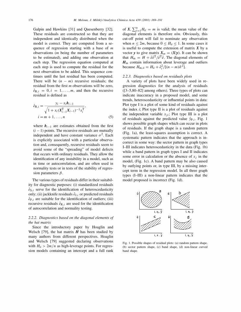
gression diagnostics for the analysis of residuals([3–5,80–82] among others). Three types of plots canindicate inaccuracy in a proposed model, and sometrends, heteroscedasticity or influential points in data:Plot type I is a plot of some kind of residuals againstthe index i; Plot type II is a plot of residuals againstthe independent variable xji ; Plot type III is a plotof residuals against the predicted value yP,i . Fig. 1shows possible graph shapes which can occur in plotsof residuals. If the graph shape is a random pattern(Fig. 1a), the least-squares assumption is correct. Asystematic pattern indicates that the approach is in-correct in some way: the sector pattern in graph typesI–III indicates heteroscedasticity in the data (Fig. 1b)while a band pattern in graph types I and II indicatessome error in calculation or the absence of xj in themodel, (Fig. 1c). A band pattern may be also causedby outlying points or, in type III, by a missing inter-cept term in the regression model. In all three graphtypes (I–III) a non-linear pattern indicates that themodel proposed is incorrect (Fig. 1d).

Fig. 1. Possible shapes of residual plots: (a) random pattern shape,(b) sector pattern shape, (c) band shape, (d) non-linear curvedband shape.


It should be noted that the plot ei against dependentvariable yi is not useful, because the two quantitiesare strongly correlated. The smaller the correlationcoefficient, the more linear is this plot.

For the identification of influential points, i.e.outliers (denoted in plots by the letter O) andhigh-leverages (denoted in plots by the letter E), vari-ous types of residuals are combined with the diagonalelements Hii of the projection hat matrix H, cf. p. 72in [1]. Most of the characteristics of influential pointsmay be expressed in the form K(m, n)×f (Hii, e

2N,i ),

where K(m, n) is a constant dependent only on m and n.

1. The graph of predicted residuals [76] has the pre-dicted residuals eP,i on the x-axis and the ordinaryresiduals ei on the y-axis. The high-leverage pointsare easily detected by their location, as they lie out-side the line y = x, and are located quite far fromthis line. The outliers are located on the line y = x,but far from its central pattern, (Fig. 2).

2. The Williams graph [76] has the diagonal elementsHii on the x-axis and the jackknife residuals eJ,ion the y-axis. Two boundary lines are drawn, thefirst for outliers, y = t0.95(n − m − 1) and thesecond for high-leverages, x = 2m/n. Note thatt0.95(n−m− 1) is the 95% quantile of the Studentdistribution with (n−m− 1) degrees of freedom,(Fig. 3).

3. The Pregibon graph [75] has the diagonal elementsHii on the x-axis and the square of normalizedresiduals e2

N,i on the y-axis. Since the expression

E(Hii + e2N,i ) = (m+ 1)/n is valid for this graph,

two different constraining lines can be drawn: y =

Fig. 2. Graph of predicted residuals: E means a high-leveragepoint and O an outlier; outliers are far from the central pattern onthe line y = x.

Fig. 3. Williams graph: E means the leverage point and O theoutlier; the first line is for outliers, y = t0.95(n − m − 1), thesecond line is for high-leverages, x = 2m/n.

−x + 2(m + 1)/n, and y = −x + 3(m + 1)/n.To distinguish among influential points the follow-ing rules are used: (a) a point is strongly influen-tial if it is located above the upper line; (b) a pointis influential if it is located between the two lines.The influential point can be either an outlier or ahigh-leverage point, (Fig. 4).

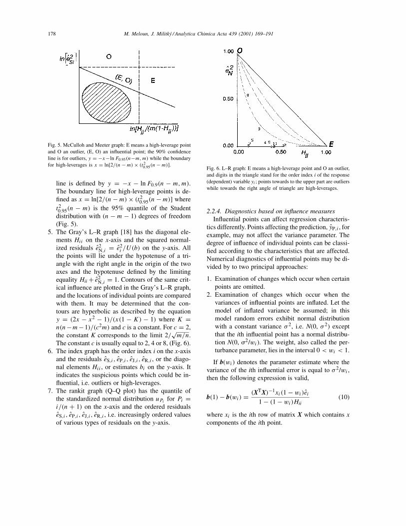
4. The McCulloh and Meeter graph [16] hasln[Hii/(m(1 − Hii))] on the x-axis and the log-arithm of square of the standardized residualsln(e2

S,i ) on the y-axis. In this plot the solid linedrawn represents the locus of points with identi-cal influence, with slope −1. The 90% confidence

Fig. 4. Pregibon graph: (E, O) are influential points, and s(E, O)are strongly influential points; two constraining lines are drawn,y = −x + 2(m + 1)/n, and y = −x + 3(m + 1)/n, the stronglyinfluential point is above the upper line; the influential point isbetween the two lines.


Fig. 5. McCulloh and Meeter graph: E means a high-leverage pointand O an outlier, (E, O) an influential point; the 90% confidenceline is for outliers, y = −x−lnF0.95(n−m,m) while the boundaryfor high-leverages is x = ln[2/(n−m)× (t20.95(n−m)].

line is defined by y = −x − lnF0.9(n − m,m).The boundary line for high-leverage points is de-fined as x = ln[2/(n−m)× (t20.95(n−m)] wheret20.95(n − m) is the 95% quantile of the Studentdistribution with (n − m − 1) degrees of freedom(Fig. 5).

5. The Gray’s L–R graph [18] has the diagonal ele-ments Hii on the x-axis and the squared normal-ized residuals e2

N,i = e2i /U(b) on the y-axis. All

the points will lie under the hypotenuse of a tri-angle with the right angle in the origin of the twoaxes and the hypotenuse defined by the limitingequality Hii + e2

N,i = 1. Contours of the same crit-ical influence are plotted in the Gray’s L–R graph,and the locations of individual points are comparedwith them. It may be determined that the con-tours are hyperbolic as described by the equationy = (2x − x2 − 1)/(x(1 − K) − 1) where K =n(n−m−1)/(c2m) and c is a constant. For c = 2,the constant K corresponds to the limit 2/

√m/n.

The constant c is usually equal to 2, 4 or 8, (Fig. 6).6. The index graph has the order index i on the x-axis

and the residuals eS,i , eP,i , eJ,i , eR,i , or the diago-nal elements Hii , or estimates bi on the y-axis. Itindicates the suspicious points which could be in-fluential, i.e. outliers or high-leverages.

7. The rankit graph (Q–Q plot) has the quantile ofthe standardized normal distribution uPi for Pi =i/(n + 1) on the x-axis and the ordered residualseS,i , eP,i , eJ,i , eR,i , i.e. increasingly ordered valuesof various types of residuals on the y-axis.

Fig. 6. L–R graph: E means a high-leverage point and O an outlier,and digits in the triangle stand for the order index i of the response(dependent) variable yi ; points towards to the upper part are outlierswhile towards the right angle of triangle are high-leverages.

2.2.4. Diagnostics based on influence measuresInfluential points can affect regression characteris-

tics differently. Points affecting the prediction, yP,i , forexample, may not affect the variance parameter. Thedegree of influence of individual points can be classi-fied according to the characteristics that are affected.Numerical diagnostics of influential points may be di-vided by to two principal approaches:

1. Examination of changes which occur when certainpoints are omitted.

2. Examination of changes which occur when thevariances of influential points are inflated. Let themodel of inflated variance be assumed; in thismodel random errors exhibit normal distributionwith a constant variance σ 2, i.e. N(0, σ 2) exceptthat the ith influential point has a normal distribu-tion N(0, �2/wi). The weight, also called the per-turbance parameter, lies in the interval 0 < wi < 1.

If b(wi) denotes the parameter estimate where thevariance of the ith influential error is equal to σ 2/wi ,then the following expression is valid,

b(1)− b(wi) = (XTX)−1xi(1 − wi)ei1 − (1 − wi)Hii

(10)

where xi is the ith row of matrix X which contains xcomponents of the ith point.


There are two limiting cases to the perturbanceparameter:

1. For wi = 1 the b(1) are equal to parameter esti-mates obtained by the LS method.

2. For wi = 0: Eq. (10) leads to the relationshipb(1) − b(0) = b − b(i), where b(i) is the estimatereached by the least-squares method with the useof all points except the ith one.

Leaving out the ith point is therefore the same as thecase when this point has unbounded infinite variance.To express the sensitivity of parameter estimates tothe perturbance parameter wi , the sensitivity functionδb(wi)/δwi can be used,

δb(wi)δwi

= (XTX)−1xi eisA + (1 − wi)Hii

s2A

(11)

where sA = 1 − (1 − wi)Hii. The following typesof sensitivity function of parameter estimates can bedefined:

1. The Jackknife influence function JCi: the sensitivityfunction of parameter estimates at the valuewi = 0is given by∣∣∣∣δb(wi)δwi

∣∣∣∣wi=0

= (XTX)−1xiei

(1 −Hii)2= JCin− 1

(12)

The term JCi is the jackknife influence function.It is related to the sensitivity function of parameterestimates, i.e. lies in the vicinity of b(0) in caseswhere the ith point is omitted, because b(0) = b(i).

2. The empirical influence function ECi: the sensi-tivity function of parameter estimates at the valuewi = 1 is given by∣∣∣∣δb(wi)δwi

∣∣∣∣wi=1

= (XTX)−1xi ei = ECin− 1

(13)

The term ECi is the empirical influence function.It is related to the sensitivity function of parameterestimates, i.e. lies in the vicinity of b(1).

3. The sample influence function SCi : the sampleinfluence function is directly proportional to thechange in the vector of parameter estimates whenthe ith point is left out. With the use of Eq. (11)we can write

SCi = n(b − b(i)) = n(XTX)−1xiei

1 −Hii(14)

All three influence functions differ only in the sin-gle term (1 −Hii), so they are not identically sen-sitive to the presence of high-leverage points, forwhichHi → 1. The disadvantage of all these influ-ence functions is that they are m-dimensional vec-tors. Their components define the influence of theith point on the estimate of the jth parameter.

2.2.5. Diagnostics based on scalar influencemeasures

Proper normalization of influence functions [23]leads to scalar measures. These measures express therelative influence of the given point on all parameterestimates.

1. The Cook measure Di directly expresses the rela-tive influence of the ith point on all parameter es-timates and has the form

Di = (b − b(i))TXTX(b − b(i))m× σ 2

= e2S,i

m× Hii

1−Hii

(15)

It is related to the confidence ellipsoid of the esti-mates but is really a shift of estimates when the ithpoint is left out. It is approximately true that whenDi > 1, the shift is greater than the 50% confi-dence region, so the relevant point is rather influ-ential. Another interpretation of Di is based on theEuclidean distance between the prediction vectoryP and the prediction vector yP,(i) estimated whenthe ith point is left out. The Cook measure Di ex-presses the influence of the ith point on the param-eter estimate b only; when the ith point does notaffect b significantly, the value of Di is low. Sucha point, however, can strongly affect the residualvariance σ 2.

2. The Atkinson measure Ai enhances the sensitivityof distance measures to high-leverage points. Thismodified version of Cook’s measure Di suggestedby Atkinson [4] is even more closely related toBelsey’s DFFITSi and has the form

Ai = |eJ,i | ×√n−mm

× Hii

1 −Hii(16)


This measure is also convenient for graphicalinterpretation; Atkinson recommends that absolutevalues of Ai be plotted in any of the ways custom-ary for residuals. With designed experiments, usu-ally Hii = m/n, and the Atkinson measure Ai isnumerically equal to the jackknife residual eJ,i .

3. The Belsey DFFITSi measure, also calledWelsch-Kuh’s distance [2], is obtained by the nor-malization of the sample influence function, andusing the variance estimate σ 2

(i) obtained fromestimates b(i). This measure has the form

DFFITS2i = e2

J,i ×Hii

1 −Hii(17)

Belsey et al. [2] suggest that the ith point is con-sidered to be significantly influential on predictionyP when DFFITSi is larger in absolute value than2√m/n.

4. The Anders–Pregibon diagnostic APi [23] ex-presses the influence of the ith point on the volumeof the confidence ellipsoid

APi = det(X∗T(i)X

∗(i))

det(X∗TX∗)(18)

where X∗ = (x/y) is the matrix having as leastcolumn the vector y. The diagnostic APi is relatedto the elements of the extended projection matrixH∗ by the expression APi = 1 − Hii − e2

N,i =1 −Hm,ii. A point is considered to be influential ifHm,ii = 1 − APi > 2(m+ 1)/n.

5. The Cook–Weisberg likelihood measure LDi [23]represents a general diagnostic defined by

LDi = 2[LΘ − L(Θ(i))] (19)

where L(Θ) is the maximum of the logarithm ofthe likelihood function when all points are usedand L(Θ)(i) is corresponding value when the ithpoint is omitted. The parametric vector Θ containseither the parameter b or the variance estimate σ 2.For strongly influential points LDi > χ2

1−α(m +1) where χ2

1−α(m + 1) is the quantile of the χ2

distribution.With the use of different variants of LDi it is

possible to examine the influence of the ith point onparameter estimates, or on the variance estimate,or on both [23]:

5.1. The likelihood measure LDi(b) examines theinfluence of individual points on the parameterestimates b by the relationship

LDi (b) = n× ln

[di ×Hii

1 −Hii+ 1

](20)

where di = e2S,i/(n−m).

5.2. The likelihood measure LDi(σ 2) examines theinfluence of individual points on the residualvariance estimates by the relationship

LDi (σ2)= n× ln

[n

n− 1

]+ n ln(1 − di)

+di(n− 1)

1 − di − 1 (21)

5.3. The likelihood measure LDi(b, σ 2) examinesthe influence of individual points on the pa-rameters b and variance estimates σ 2 togetherby the relationship

LDi (b, σ 2)= n× ln

[n

n− 1

]+ n ln(1 − di)

+ di(n− 1)

(1 − di)(1 −Hii)− 1 (22)

6. Hadi’s influence measure [22] is a new measure andgraphical display for the characterization of overallpotential influence in linear regression models. Thisinfluence measure is based on the simple fact thatpotentially influential observations are outliers inthe X- or y-space. This measure is expressed in theform

K2i = m

1 −Hii

e2N,i

1 − e2N,i

+ Hii

1 −Hii(23)

where eN,i is ith normalized residual. Large K2i

indicates influential points; the potential residualplot is then the scatter plot of the first versus sec-ond components of K2

i . This plot is related but notequivalent to the L–R plot. The extensions of K2

i

for the identification of influential subsets is verysimple [22].


3. Procedure

3.1. Procedure for regression model building

The procedure for regression model building includ-ing the examination of influential points comprises thefollowing steps:

Step 1. Proposal of a model: the procedure usuallystarts from the simplest model, with individual ex-planatory controllable variables not raised to powersother than the first, and with no interaction terms ofthe type xj xk included.

Step 2. Exploratory data analysis in regression: thescatter plot of individual variables and all the possiblepair combinations are examined. Also in this step,the influential points causing multicollinearity aredetected.

Step 3. Parameter estimation: the parameters ofthe proposed regression model and the correspond-ing basic statistical characteristics of this model aredetermined by the classic least-squares method (LS).Individual parameters are tested for significance byway of Student’s t-test. The mean quadratic errorof prediction MEP and the Akaike information cri-terion AIC are calculated to examine the quality ofmodel.

Step 4. Analysis of regression diagnostics: dif-ferent diagnostic graphs and numerical measuresare used to examine influential points, namely out-liers and high-leverages. If influential points arefound, it has to be decided whether these pointsshould be eliminated from the data. If pointsare eliminated, the whole data treatment must berepeated.

Step 5. Construction of a more accurate model: ac-cording to the test for fulfillment of the conditionsfor the least-squares method, and the result of regres-sion diagnostics, a more accurate regression model isconstructed.

3.2. Software used

For the creation of regression diagnostic graphs andthe computation of all regression characteristics analgorithm was written in Matlab 5.3 and also a uniquemodule of the ADSTAT package was used, cf. [86].The matrix oriented programming leads here to thevery effective computations.

4. Illustrative examples

Regression model building and the discovery of in-fluential points in three datasets from literature havebeen investigated extensively. These data are suitablefor a demonstration of the efficiency of diagnostictools for influential points indication. The majority ofmultiple outliers and high-leverages has been betterdetected by diagnostic plots than by values in tables.

Example 1. Operation of a plant for the oxidationof ammonia to nitric acid: the stackloss dataset, orig-inally studied by Brownlee [11], is by far the mostoften cited sample data in the regression diagnosticliterature: these are observations from 21 days in theoperation of a plant for the oxidation of ammoniaas a stage in the production of nitric acid. The inde-pendent variables are: x1 the rate of operation of theplant measured by air flow, x2 the inlet temperatureof the cooling water circulating through coils in thecountercurrent absorption tower for nitric acid, x3proportional to the concentration of nitric acid in theabsorbing liquid in the tower expressed as 10 × (acidconcentration − 50), and dependent variable y rep-resenting the stack loss, i.e. 10 times the percentageof ingoing ammonia escaping unconverted as unab-sorbed nitric oxides. This is an inverse measure of theyield of nitric acid for the plant Table 1.

These data have been much analyzed as a tested formethods of outlier and leverage detection. A summaryof many analyses is given by Atkinson, p. 266 [4].While Gray and Ling [19] identified the subset (1, 2,3) as the most influential triple in the stackloss data,other authors described the joint influential points (1,2, 3, 4, 21). Investigation of plant operations indicatesthat the following sets of runs can be considered asreplicates: (1, 2), (4, 5, 6), (7, 8), (11, 12) and (18, 19).While the runs in each set are not exact replicates, thepoints are sufficiently close to each other in x-spacefor them to be used as such.

As the conditioning number K = λmax/λmin (theratio of the maximal and minimal eigenvalue of the re-gressor matrix X) was 9.99 which was less than 1000,no multicollinearity was proven. Also, all three val-ues of the variance inflation factor VIF = 2.87, 2.40and 1.41 of matrix X were less than 10, so no multi-collinearity was indicated.


Table 1The stackloss dataset written in the order x1, x2, x3, y

80.0 27.0 89.0 42.0 80.0 27.0 88.0 37.0 75.0 25.0 90.0 37.062.0 24.0 87.0 28.0 62.0 22.0 87.0 18.0 62.0 23.0 87.0 18.062.0 24.0 93.0 19.0 62.0 24.0 93.0 20.0 58.0 23.0 87.0 15.058.0 18.0 80.0 14.0 58.0 18.0 89.0 14.0 58.0 17.0 88.0 13.058.0 18.0 82.0 11.0 58.0 19.0 93.0 12.0 58.0 18.0 89.0 8.050.0 18.0 86.0 7.0 50.0 19.0 72.0 8.0 50.0 19.0 79.0 8.050.0 20.0 80.0 9.0 56.0 20.0 82.0 15.0 70.0 20.0 91.0 15.0

The stackloss data have been re-examined to showthe detection power of various regression diagnosticsfor influential points detection. This analysis beginsby fitting a model in the three explanatory variablesto the untransformed data. The majority of the par-tial correlation coefficients between the percentage ofthe input ammonia and chemical descriptors were sig-nificant; therefore, the total OLS regression model isdetermined

y = −37.68(12.01,S)+ 0.7336(0.1388,S)x1

+1.3883(0.3565,S)x2 − 0.2167(0.1613,N)x3

where brackets contain the standard deviation of theparameter estimated. The quantile t1−α/2(21–4) =

Fig. 7. Diagnostics based on residual plots and hat matrix elements for stackloss data: (a) graph of predicted residuals, (b) Williams graph,(c) Pregibon graph, (d) McCulloh and Meeter graph, (e) Gray L–R graph, (f) rankit Q–Q graph of jackknife residuals.

2.110 of the Student’s t-test (5% significance level)is used to examine the test statistics (t’s) of the in-dividual regression parameters: t0 = −3.137, t1 =5.285, t2 = 3.894, t3 = −1.343. All values exceptt3 are equal to or greater than t1−α/2(21–4) = 2.110and are significant, denoted with the letter S, whilefor b3 the letter N stands for non-significant. Themodel is described with the mean error of predictionMEP = 13.61, the predicted coefficient of deter-mination R2

P = 0.9283 and the Akaike informationcriterion AIC = 53.09 (Figs. 7 and 8).

Detecting influential points, three blocks of diag-nostics have been applied: (i) diagnostic plots basedon residuals and hat matrix elements, (ii) index graphsof diagnostics based on vector and scalar influence


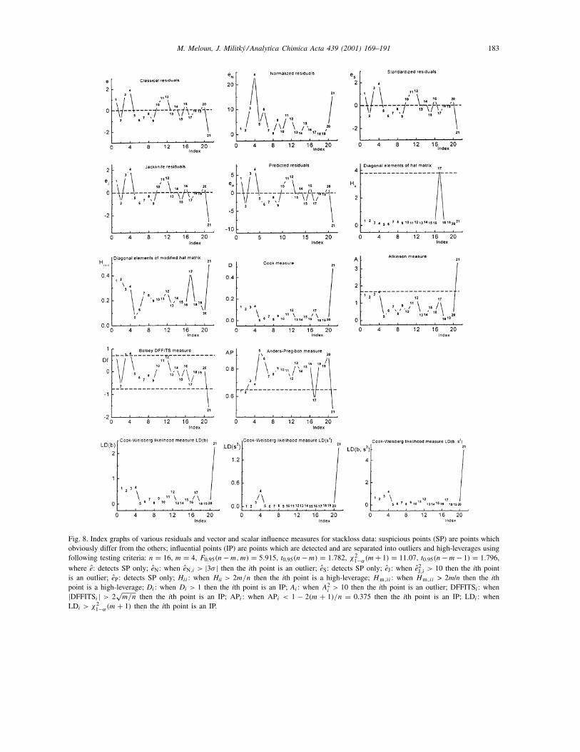
Fig. 8. Index graphs of various residuals and vector and scalar influence measures for stackloss data: suspicious points (SP) are points whichobviously differ from the others; influential points (IP) are points which are detected and are separated into outliers and high-leverages usingfollowing testing criteria: n = 16, m = 4, F0.95(n−m,m) = 5.915, t0.95(n−m) = 1.782, χ2

1−α(m+ 1) = 11.07, t0.95(n−m− 1) = 1.796,where e: detects SP only; eN: when eN,i > |3σ | then the ith point is an outlier; eS: detects SP only; eJ: when e2

J,i > 10 then the ith pointis an outlier; eP: detects SP only; Hii : when Hii > 2m/n then the ith point is a high-leverage; Hm ,ii : when Hm ,ii > 2m/n then the ithpoint is a high-leverage; Di : when Di > 1 then the ith point is an IP; Ai : when A2

i > 10 then the ith point is an outlier; DFFITSi : when|DFFITSi | > 2

√m/n then the ith point is an IP; APi : when APi < 1 − 2(m + 1)/n = 0.375 then the ith point is an IP; LDi : when

LDi > χ21−α(m+ 1) then the ith point is an IP.


Table 2A survey of the influential points which were tested using various diagnostic toolsa

Diagnostic indicating SP and IP Suspicious points (SP) Influential points (IP) Outliers (O) High-leverages (E)

(A) Diagnostical plots based on residuals and hat matrix elements1. Graph of predicted residuals 1, 3, 4, 11, 12, 21 2, 3, 4, 17, 21 3, 4, 21 1, 2, 172. Williams graph 4, 17, 21 4, 17, 21 4, 21 173. Pregibon graph 17, 21 17, 21 – –4. McCulloh–Meeter graph 4, 17, 21 4, 17, 21 4, 21 175. Gray’s L–R graph 1, 2, 4, 17, 21 1, 2, 4, 17, 21 4, 21 1, 2, 176. Q–Q graph of jackknife residuals 1, 3, 4, 11, 12, 21 – – –

(B) Diagnostics based on scalar and vector influence measures7. Cook measure D 1, 2, 3, 4, 21 21 – –8. Atkinson measure A 1, 2, 3, 4, 17, 21 4, 21 – –9. Belsey measure DFFITS 1, 2, 3, 4, 12, 17, 21 4, 21 – –10. Anders–Pregibon diagnostic AP 1, 2, 17, 21 1, 2, 17, 21 – –11. Cook–Weisberg likelihood measure LD(b) 1, 2, 3, 4, 12, 17, 21 21 – –12. Cook–Weisberg likelihood measure LD(s2) 4, 21 21 – –13. Cook–Weisberg likelihood measure LD(b, s2) 4, 21 21 – –

(C) Index graphs of residuals and hat matrix elements14. Ordinary residuals e 1, 3, 4, 21 21 – –15. Normalized residuals eN 4, 21 4, 21 – –16. Standardized residuals eS 4, 12, 21 4, 21 – –17. Jackknife residuals eJ 1, 4, 21 21 – –18. Predicted residuals eP 1, 3, 4, 21 4, 21 – –19. Diagonal elements of hat matrix Hii 17 17 – –20. Diagonal elements of modified hat matrix Hm,ii 1, 2, 17, 21 2, 17, 21 – –

a Suspicious points (SP) are points in diagnostic graphs which obviously differ from the others; influential points (IP) are pointswhich are detected and are separated into outliers and high-leverages using following testing criteria: n = 16,m = 4, F0.95(n − m,m) =5.915, t0.95(n−m) = 1.782, χ2

1−α(m+ 1) = 11.07, t0.95(n−m− 1) = 1.796.

measures, and (iii) index graphs of residuals and hatmatrix elements. Table 2 shows that five diagnosticplots and the Q–Q graph of the jackknife residu-als indicate suspicious points which obviously differfrom others. The statistical criteria in the diagnos-tic plots were then used to prove influential points.These plots also separate influential points into out-liers and high-leverages. The diagnostic plots foundtwo outliers, 4 and 21, and one high-leverage point,17. Index graphs of diagnostics based on vector andscalar influence measures, as well as index graphsof residuals and hat matrix elements, tested all thesuspicious points and found statistically significantinfluential points. However, these index graphs arenot able to separate these points into outliers andhigh-leverages. Most index graphs agreed that therewere three influential points (4, 17, 21). Removinga non-significant regressor from the equation has anegligible effect on the fitted values and deletion ofone outlier (21) formed the regression model

y = −53.21(4.55,S)+ 0.824(0.123,S)x1

+0.999(0.336,S)x2

with MEP = 9.35, R2P = 0.9536 and AIC = 43.80,

while when deleting 2 outliers (4, 21) the final re-gression model achieved was

y = −52.28(3.86,S)+ 0.888(0.106,S)x1

+0.756(0.297,S)x2

with MEP = 6.94, R2P = 0.9656 and AIC = 35.30.

The lowest values of MEP and AIC and the highestvalue of R2

P proved, to be the final model. On its own,the leverage 17 is not particularly informative aboutthe behavior of the units, since it does not depend onthe observed values of y.

Example 2. Aerial biomass and five physicochemicalproperties of the substrate (salinity, pH, K, Na andZn) [67]: the purpose is to find a regression model


to detect influential points and to identify importantsoil characteristics (salinity, pH, K, Na and Zn) in-fluencing the aerial biomass production of the marshgrass Spartina alterniflora. The 45 data values used in-volve 1 month of sampling are part of a larger studyby Linthurst (cf. p. 161 in [84,85]) and five substratemeasurements: x1 salinity (‰), x2 acidity as measuredin water pH, x3 potassium (ppm), x4 sodium (ppm),and x5 zinc (ppm); y the dependent variable is aerialbiomass (g/m2), (Table 3).

The purpose of this study was to identify the im-portant soil characteristics influencing aerial biomassproduction of the marsh grass and to identify the sub-strate variables showing the stronger relationship tobiomass to relate total variability in biomass produc-tion to total variability in the five substrate variables.

The initial model assumes the biomass, y, can beadequately characterized by linear relationship withthe five independent variables plus an intercept,

y = β0 + β1x1 + β2x2 + β3x3 + β4x4 + β5x5

where y is the vector of biomass measurements and X(45 × 6) consists of the column vector 1, the 45 × 1column vector of ones, and the five column vectors ofdata for substrate variables.

As the conditioning number K = λmax/λmin (theratio of the maximal and minimal eigenvalue of theregressor matrix X) was 17.791 which was less than1000, no multicollinearity was proven. Also, all fivevalues of the variance inflation factor VIF = 2.217,3.331, 2.983, 3.334 and 4.310 of matrix X were lessthan 10, and thus no multicollinearity was indicated.The OLS method found the regression model

y = 1252.3(1234.8,N)− 30.3(24.0,N)x1

+305.5(87.9,S)x2 − 0.285(0.348,N)x3

−0.00867(0.01593,N)x4 − 20.68(15.06,N)x5

where brackets contain the standard deviations of theparameters estimated. The quantile t1−α/2(45–6) =2.023 of a Student’s t-test (5% significance level) wasused to examine the test statistics (t’s) of the individualregression parameters: t0 = 1.014, t1 = −1.260, t2 =3.477, t3 = −0.818, t4 = −0.544 and t5 = −1.373.All values except t2 are less than t1−α/2(45–6) =2.023, are not significant, and are denoted by the let-ter N. The model was described with a mean error of

Table 3Aerial biomass and five physicochemical properties of the substrate[67]a

x1 x2 x3 x4 x5 y

33 5.00 1441.67 35185.50 16.4524 67635 4.75 1299.19 28170.40 13.9852 51632 4.20 1154.27 26455.00 15.3276 105230 4.40 1045.15 25072.90 17.3128 86833 5.55 521.62 31664.20 22.3312 100833 5.05 1273.02 25491.70 12.2778 43636 4.25 1346.35 20877.30 17.8225 54430 4.45 1253.88 25621.30 14.3516 68038 4.75 1242.65 27587.30 13.6826 64030 4.60 1281.95 26511.70 11.7566 49230 4.10 553.69 7886.50 9.8820 98437 3.45 494.74 14596.00 16.6752 140033 3.45 525.97 9826.80 12.3730 127636 4.10 571.14 11978.40 9.4058 173630 3.50 408.64 10368.60 14.9302 100430 3.25 646.65 17307.40 31.2865 39627 3.35 514.03 12822.00 30.1652 35229 3.20 350.73 8582.60 28.5901 32834 3.35 496.29 12369.50 19.8795 39236 3.30 580.92 14731.90 18.5056 23630 3.25 535.82 15060.60 22.1344 39228 3.25 490.34 11056.30 28.6101 26831 3.20 552.39 8118.90 23.1908 25231 3.20 661.32 13009.50 24.6917 23635 3.35 672.15 15003.70 22.6758 34029 7.10 528.65 10225.00 0.3729 243635 7.35 563.13 8024.20 0.2703 221635 7.45 497.96 10393.00 0.3205 209630 7.45 458.38 8711.60 0.2648 166030 7.40 498.25 10239.60 0.2105 227226 4.85 936.26 20436.00 18.9875 82429 4.60 894.79 12519.90 20.9687 119625 5.20 941.36 18979.00 23.9841 196026 4.75 1038.79 22986.10 19.9727 208026 5.20 898.05 11704.50 21.3864 176425 4.55 989.87 17721.00 23.7063 41226 3.95 951.28 16485.20 30.5589 41626 3.70 939.83 17101.30 26.8415 50427 3.75 925.42 17849.00 27.7292 49227 4.15 954.11 16949.60 21.5699 63624 5.60 720.72 11344.60 19.6531 175627 5.35 782.09 14752.40 20.3295 123226 5.50 773.30 13649.80 19.5880 140028 5.50 829.26 14533.00 20.1328 152028 5.40 856.96 16892.20 19.2420 1560

a The 45 data values used involve 1 month of samplingare part of a larger study by Linthurst (cf. p. 161 in [84,85])and five substrate measurements: x1 salinity (‰), x2 acidity asmeasured in water pH, x3 potassium (ppm), x4 sodium (ppm),and x5 zinc (ppm); y the dependent variable is aerial biomass(g/m2).


Fig. 9. Selected diagnostics plots for the detection of influential points in aerial biomass data: (a) Williams graph, (b) graph of predictedresiduals, (c) Gray L–R graph, (d) index graph of Atkinson measure, (e) index graph of diagonal elements of the hat matrix, (f) rankitQ–Q graph of jackknife residuals.

prediction MEP = 1.7678 × 105, the predicted coef-ficient of determination R2

P = 0.7649 and the Akaikeinformation criterion AIC = 544.40.

Fig. 9 shows six reliable diagnostic graphs for thedetection of influential points. While the first threegraphs separate outliers from high-leverages, the otherthree graphs indicate influential points only withouttheir separation: 7 influential points were detected in45 data values, and separated into five outliers (12,14, 29, 33, 34) and two high-leverages (5, 7). Thet-test of the partial regression parameters H0: βj = 0would seem to suggest that four of the five independentvariables are unimportant and could be dropped fromthe model. The corrected regression model was thenre-calculated using a data set without five outliers 12,14, 29, 33 and 34 and without statistically insignificantparameters in the form

y = −1133.0(198.15,S)+ 447.5(42.1,S)x2

with MEP = 1.0633 × 105, R2P = 0.8527 and AIC =

463.67. The lowest values of MEP and AIC and thehighest value of R2

P proved, to be the best final model.

Example 3. The quantitative structure-activity rela-tionship analysis of positively charged sulfonamide

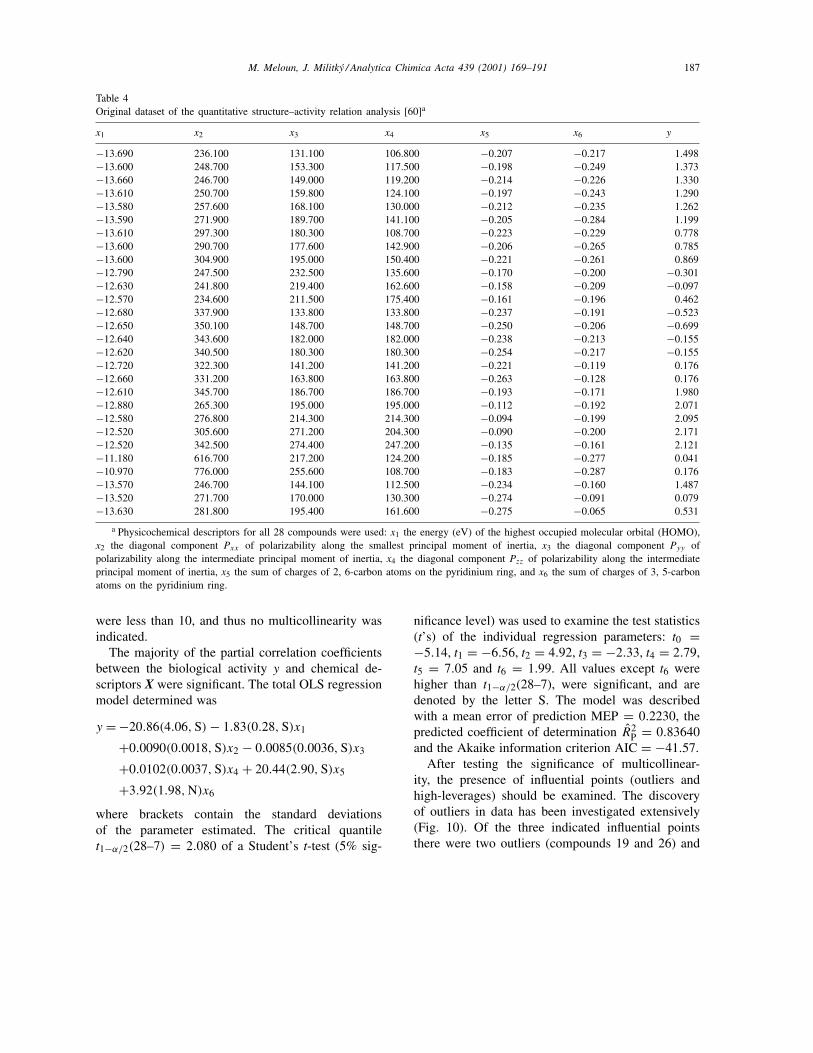
inhibitors of the zinc enzyme carbonic anhydride [60].The synthetic routes of a series of tri-, tetra-, andpenta-substituted 1-2(sulfonamido-1,3,4-thiadiazol-5-yl) pyridinium agents have been published [60].The 50% inhibitory concentration [�M] of carbonicanhydrase for 28 compounds was determined, trans-formed by natural logarithm and signified by thedependent variable y. A number of physicochemicaldescriptors for all 28 compounds were used: x1 theenergy (eV) of the highest occupied molecular orbital(HOMO), x2 the diagonal component Pxx of polariz-ability along the smallest principal moment of inertia,x3 the diagonal component Pyy of polarizability alongthe intermediate principal moment of inertia, x4 thediagonal component Pzz of polarizability along theintermediate principal moment of inertia, x5 the sumof charges of 2, 6-carbon atoms on the pyridiniumring, and x6 the sum of charges of 3, 5-carbon atomson the pyridinium ring, Table 4.

As the conditioning number K = λmax/λmin (theratio of the maximal and minimal eigenvalue of theregressor matrix X) was 36.461, which was less than1000, no multicollinearity was proven. Also, all sixvalues of the variance inflation factor VIF of matrix X


Table 4Original dataset of the quantitative structure–activity relation analysis [60]a

x1 x2 x3 x4 x5 x6 y

−13.690 236.100 131.100 106.800 −0.207 −0.217 1.498−13.600 248.700 153.300 117.500 −0.198 −0.249 1.373−13.660 246.700 149.000 119.200 −0.214 −0.226 1.330−13.610 250.700 159.800 124.100 −0.197 −0.243 1.290−13.580 257.600 168.100 130.000 −0.212 −0.235 1.262−13.590 271.900 189.700 141.100 −0.205 −0.284 1.199−13.610 297.300 180.300 108.700 −0.223 −0.229 0.778−13.600 290.700 177.600 142.900 −0.206 −0.265 0.785−13.600 304.900 195.000 150.400 −0.221 −0.261 0.869−12.790 247.500 232.500 135.600 −0.170 −0.200 −0.301−12.630 241.800 219.400 162.600 −0.158 −0.209 −0.097−12.570 234.600 211.500 175.400 −0.161 −0.196 0.462−12.680 337.900 133.800 133.800 −0.237 −0.191 −0.523−12.650 350.100 148.700 148.700 −0.250 −0.206 −0.699−12.640 343.600 182.000 182.000 −0.238 −0.213 −0.155−12.620 340.500 180.300 180.300 −0.254 −0.217 −0.155−12.720 322.300 141.200 141.200 −0.221 −0.119 0.176−12.660 331.200 163.800 163.800 −0.263 −0.128 0.176−12.610 345.700 186.700 186.700 −0.193 −0.171 1.980−12.880 265.300 195.000 195.000 −0.112 −0.192 2.071−12.580 276.800 214.300 214.300 −0.094 −0.199 2.095−12.520 305.600 271.200 204.300 −0.090 −0.200 2.171−12.520 342.500 274.400 247.200 −0.135 −0.161 2.121−11.180 616.700 217.200 124.200 −0.185 −0.277 0.041−10.970 776.000 255.600 108.700 −0.183 −0.287 0.176−13.570 246.700 144.100 112.500 −0.234 −0.160 1.487−13.520 271.700 170.000 130.300 −0.274 −0.091 0.079−13.630 281.800 195.400 161.600 −0.275 −0.065 0.531

a Physicochemical descriptors for all 28 compounds were used: x1 the energy (eV) of the highest occupied molecular orbital (HOMO),x2 the diagonal component Pxx of polarizability along the smallest principal moment of inertia, x3 the diagonal component Pyy ofpolarizability along the intermediate principal moment of inertia, x4 the diagonal component Pzz of polarizability along the intermediateprincipal moment of inertia, x5 the sum of charges of 2, 6-carbon atoms on the pyridinium ring, and x6 the sum of charges of 3, 5-carbonatoms on the pyridinium ring.

were less than 10, and thus no multicollinearity wasindicated.

The majority of the partial correlation coefficientsbetween the biological activity y and chemical de-scriptors X were significant. The total OLS regressionmodel determined was

y = −20.86(4.06,S)− 1.83(0.28,S)x1

+0.0090(0.0018,S)x2 − 0.0085(0.0036,S)x3

+0.0102(0.0037,S)x4 + 20.44(2.90,S)x5

+3.92(1.98,N)x6

where brackets contain the standard deviationsof the parameter estimated. The critical quantilet1−α/2(28–7) = 2.080 of a Student’s t-test (5% sig-

nificance level) was used to examine the test statistics(t’s) of the individual regression parameters: t0 =−5.14, t1 = −6.56, t2 = 4.92, t3 = −2.33, t4 = 2.79,t5 = 7.05 and t6 = 1.99. All values except t6 werehigher than t1−α/2(28–7), were significant, and aredenoted by the letter S. The model was describedwith a mean error of prediction MEP = 0.2230, thepredicted coefficient of determination R2

P = 0.83640and the Akaike information criterion AIC = −41.57.

After testing the significance of multicollinear-ity, the presence of influential points (outliers andhigh-leverages) should be examined. The discoveryof outliers in data has been investigated extensively(Fig. 10). Of the three indicated influential pointsthere were two outliers (compounds 19 and 26) and


Fig. 10. Selected diagnostics plots for the detection of influential points in structure–activity data: (a) Williams graph, (b) graph of predictedresiduals, (c) Gray L–R graph, (d) index graph of Atkinson measure, (e) index graph of diagonal elements of the hat matrix, (f) rankitQ–Q graph of jackknife residuals.

one high-leverage point (compound 25). While Mager[60] found two high-leverage points (compounds25 and 28), one outlier (compound 19), and twocollinearity-creating points (compounds 24 and 25),but he found no influential points; despite Mager’sconclusion [60], with the use of graphical diagnosticsthree influential points (compound 19, 25 and 26)were detected and separated into two outliers (com-pounds 19 and 26) which should be excluded from theoriginal dataset, and one high-leverage (compound25) which can remain in the data.

With the omission of one insignificant regressor x6and the deletion of two outliers (19, 26) the regressionmodel was

y = −20.51(3.39,S)− 1.67(0.23,S)x1

+0.0074(0.0014,S)x2 − 0.0058(0.0031,N)x3

+0.0113(0.0030,S)x4 + 17.18(2.07,S)x5

where brackets contain the standard deviation of pa-rameter estimated. The quantile t1−α/2(26–6) = 2.086of a Student’s t-test (5% significance level) was usedto examine the test statistics (t’s) of the individual

regression parameters: t0 = −6.06, t1 = −7.43,t2 = 5.17, t3 = −1.88, t4 = 3.70, and t5 = 8.29.All values except t3 were higher than t1−�/2(26–6),were significant, and are denoted by the letter S. Themodel was described with a mean error of predictionMEP = 0.1586, the predicted coefficient of deter-mination R2

P = 0.8831 and the Akaike informationcriterion AIC = −48.37.

With the omission of another insignificant regressorx3 the final regression model was

y = −20.48(3.58,S)− 1.61(0.24,S)x1

+0.0063(0.0014,S)x2 + 0.0085(0.0028,S)x4

+15.00(1.82,S)x5

and the critical quantile t1−α/2(26–5) = 2.080 ofa Student’s t-test (5% significance level) was usedto examine the test statistics (t’s) of the individualregression parameters: t0 = −5.71, t1 = −6.84,t2 = 4.56, t4 = 3.01 and t5 = 8.24. All valueswere significant, and are denoted by the letter S.The model was described with a mean error of pre-diction MEP = 0.1746, the predicted coefficient of


determination R2P = 0.8703 and the Akaike informa-

tion criterion AIC = −46.142.

5. Conclusions

Regression diagnostics do not require a knowledgeof an alternative hypothesis for the testing or fulfillingof the other assumptions of classical statistical tests.In the interactive PC-assisted diagnosis of data, theexamination of data quality involves the detection ofinfluential points, outliers and high-leverages, whichcause many problems in regression analysis by shift-ing the parameter estimates or increasing the varianceof the parameters. The main difference between theuse of regression diagnostics and classical statisticaltests is that there is no necessity for an alternativehypothesis, but all kinds of deviations from the idealstate are discovered. In statistical graphics, informa-tion is contained in observable shapes and patterns:regression diagnostics represent the graphical pro-cedures and numerical measures for an examinationof the regression triplet, i.e. the identification of (i)the data quality for a proposed model, (ii) the modelquality for a given dataset, and (iii) a fulfillment ofall least-squares assumptions. The authors’ conceptof exploratory regression analysis is based on thefacts that “the user knows more about the data thanthe computer does” and graphs are more informativethan tables. Selected diagnostic plots were chosen assuitable to give reliable results of influential pointsdetection and to separate influential points into out-liers and high-leverages. The graphical aids for theidentification of outliers and high-leverage points arecombined with graphs for the identification of in-fluence type based on likelihood distance. All thesegraphically oriented techniques are suitable for therapid estimation of influential points, but are gener-ally incapable of solving problems with masking andswamping. The Matlab 5.3 procedure for influentialpoints characteristics computation is very useful forpractitioners and can be used very simply for routinecalculations. Results are comparable with those ob-tained with the use of expensive statistical packages.

Acknowledgements

The financial support of the Grant Agency of theCzech Republic (Grant no. 303/00/1559) is gratefully

acknowledged. Karel Kupka is acknowledged for hishelp with some figures made in ADSTAT 3.0.

References

[1] M. Meloun, J. Militký, M. Forina, Chemometrics forAnalytical Chemistry, Vol. 2, PC-Aided Regression andRelated Methods, Ellis Horwood, Chichester, 1994.

[2] D.A. Belsey, E. Kuh, R.E. Welsch, Regression Diagnostics:Identifying Influential data and Sources of Collinearity, Wiley,New York, 1980.

[3] R.D. Cook, S. Weisberg, Residuals and Influence inRegression, Chapman & Hall, London, 1982.

[4] A.C. Atkinson, Plots, Transformations and Regression: AnIntroduction to Graphical Methods of Diagnostic RegressionAnalysis, Claredon Press, Oxford, 1985.

[5] S. Chatterjee, A.S. Hadi, Sensitivity Analysis in LinearRegression, Wiley, New York, 1988.

[6] V. Barnett, T. Lewis, Outliers in Statistical Data, 2nd Edition,Wiley, New York, 1984.

[7] R.E. Welsch, Linear regression diagnostics, Technical Report923-77, Sloan School of Management, Massachusetts Instituteof Technology, 1977.

[8] R.E. Welsch, S.C. Peters, Finding influential subsets of datain regression models, in: A.R. Gallant, T.M. Gerig (Eds.),Proceedings of the 11th Interface Symposium on ComputerScience and Statistics, Institute of Statistics, North carolinaState University, Raleigh, 1978.

[9] S. Weisberg, Applied Linear Regression, Wiley, New York,1985.

[10] P.J. Rousseeuw, A.M. Leroy, Robust Regression and OutlierDetection, Wiley, New York, 1987.

[11] K.A. Brownlee, Statistical Theory and Methodology inScience and Engineering, Wiley, New York, 1965.

[12] J.F. Gentleman, M.B. Wilk, Detecting outliers. II.Supplementing the direct analysis of residuals, Biometrics 31(1975) 387–410.

[13] R.D. Cook, Detection of influential observations in linearregression, Technometrics 19 (1977) 15–18.

[14] R.D. Cook, S. Weisberg, Characterization of an empiricalinfluence function for detecting influential cases in regression,Technometrics 22 (1980) 495–508.

[15] D.C. Hawkins, D. Bradu, G.V. Kass, Location of severaloutliers in multiple regression data using elemental sets,Technometrics 26 (1984) 197–208.

[16] C.E. McCulloch, D. Meeter, Discussion of “outliers” by R.J.Beckman and R.D. Cook, Technometrics 25 (1983) 152–155.

[17] J.B. Gray, The L–R plot: a graphical tool for assessinginfluence, in: Proceedings of the Statistical ComputingSection, Vols. 159–164, American Statistical Association,1983.

[18] J.B. Gray, Graphics for regression diagnostics, Proceedings ofthe Statistical Computing Section, Vols. 102–107, AmericanStatistical Association, 1985.

[19] J.B. Gray, R.F. Ling, K-clustering as a detection tool forinfluential subsets in regression, Technometrics 26 (1984)305–330.


[20] J.B. Gray, A classification of influence measures, J. Statist.Comput. Simul. 30 (1988) 159–171.

[21] J.B. Gray, A simple graphic for assessing influence inregression, J. Statist. Comput. Simul. 24 (1986) 121–134.

[22] A.S. Hadi, A new measure of overall potential influence inlinear regression, Comput. Statist. Data Anal. 14 (1992) 1–27.

[23] F.R. Hampel, The influence curve and its role in robustestimation, J. Am. Statist. Assoc. 69 (1974) 383–393.

[24] R.D. Cook, Influential observation in linear regression, J. Am.Statist. Assoc. 74 (1979) 169–174.

[25] R.D. Cook, P. Prescot, On the accuracy of Bonferronisignificance levels for detecting outliers in linear models,Technometrics 23 (1981) 59.

[26] D.F. Andrews, D. Pregibon, Finding outliers that matter, J.Roy. Statist. Soc. B 40 (1978) 85–93.

[27] S. Weisberg, Developments in linear-regression methodology:1959–1982 discussion, Technometrics 25 (1983) 240–244.

[28] D.A. Pierce, R.J. Gray, Testing normality of errors inregression models, Biometrika 69 (1982) 233.

[29] A. Hedayat, D.S. Robson, Independent stepwise residuals fortesting homoscedasticity, J. Am. Statist. Assoc. 65 (1970)1573.

[30] R.L. Brown, J. Durbin, J.M. Evans, Techniques for testingthe constancy of regression relationship over time, J. Roy.Statist. Soc., Ser. B 37 (1975) 149.

[31] J.S. Galpin, D.M. Hawkins, The use of recursive residualsin checking model fit in linear regression, Am. Statist. 68(1973) 144.

[32] C.P. Quesenberry, Some transformation methods ingoodness-of-fit, in: R.B. D’Agostino, M.A. Stephens (Eds.),Goodness of Fit Techniques, Marcel Dekker, New York,Chapter 6, 1986.

[33] R.E. Welsch, Influence functions and regression diagnostics,in: R. Launer, A. Siegel (Eds.), Modern Data Analysis,Academic Press, New York, 1982.

[34] S. Chaterjee, A.S. Hadi, Influential observations,high-leverage points, and outliers in linear regression (withdiscussion), Statist. Sci. 1 (1986) 379–416.

[35] J. Militký, in: Proceedings of the European SimulationConference 87, Prague, September 1987.

[36] M.A. O’Gorman, R.M. Myers, Commun. Statist. 16 (1987)771.

[37] A.S. Hadi, Diagnosting collinearity — influentialobservations, Comput. Statist. Data Anal. 7 (1988) 143–159.

[38] A.S. Hadi, Two graphical displays for the detection ofpotentially influential subsets in regression, J. Appl. Statist.17 (1990) 313–327.

[39] S. Ghosh, On two methods of identifying influential sets ofobservations, Statist. Probability Lett. 7 (1989) 241–245.

[40] R.D. Cook, S. Weisberg, Regression diagnostics with dynamicgraphics, Technometrics 31 (1989) 277–311.

[41] S.R. Paul, K.Y. Fung, A generalized extreme studentizedresidual multiple-outlier detection procedure in linearregression, Technometrics 33 (1991) 339–348.

[42] P.J. Rousseeuw, B.C. van Zomeren, Unmasking multivariateoutliers and leverage points, J. Am. Statist. Assoc. 85 (1990)871–880.

[43] A.S. Hadi, W.D. Jones, R.F. Ling, A unifying representationof some case-deletion influence measures in univariate andmultivariate linear regression, J. Statist. Planning Inference46 (1995) 123–135.

[44] B. Seaver, K. Triantis, The identification of influential subsetsin regression using a fuzzy clustering strategy, Technometrics41 (1999) 340–352.

[45] Y. Dodge, A.S. Hadi, Simple graphs and bounds for theelements of the hat matrix, J. Appl. Statist. 26 (1999)817–823.

[46] R.D. Cook, F. Critchley, Identifying regression outliersand mixtures graphically, J. Am. Statist. Assoc. 95 (2000)781–794.

[47] SAS Institute Inc., SAS/STAT User’s Guide, Version 6, 4thEdition, Vol. II, SAS Institute Inc., Cary, NC, 1989.

[48] Y. Tanaka, F. Zhang, R-mode and Q-mode influence analysesin statistical modelling: relationship between influencefunction approach and local influence approach, Comput.Statist. Data Anal. 32 (1999) 197–218.

[49] A.S. Kosinski, A procedure for the detection of multivariateoutliers, Comput, Statist. Data Anal. 29 (1999) 145–161.

[50] W.K. Fung, Graphical summaries for influence of multipleobservations, Commun. Statist. — Theory Methods 24 (1995)415–427.

[51] B.E. Barrett, R.F. Ling, General classes of influence measuresfor multivariate regression, J. Am. Statist. Assoc. 87 (1992)184–191.

[52] A.S. Hadi, J.S. Simonoff, Procedures for the identification ofmultiple outliers in linear models, J. Am. Statist. Assoc. 88(1993) 1264–1272.

[53] S.S. Gupta, D.-Y. Huang, On detecting influential data andselecting regression variables, J. Statist. Planning Inference53 (1996) 421–435.

[54] Ch. Kim, Cook’s distance in spline smoothing, Statist.Probability Lett. 31 (1996) 139–144.

[55] A. Singh, Outliers and robust procedures in somechemometric applications, Chemomet. Intelligent Lab. Syst.33 (1996) 75–100.

[56] Y.Z. Liang, O.M. Kvalheim, Robust methods for multivariateanalysis: a tutorial review, Chemomet. Intelligent Lab. Syst.32 (1996) 1–10.

[57] W.K. Fung, A stepwise method for the identification ofmultiple outliers and influential observations, S. Afr. Statist.J. 29 (1995) 51–64.

[58] F. Kianifard, W.H. Swallow, A review of the developmentand application of recursive residuals in linear models, J. Am.Statist. Assoc. 91 (1996) 391–400.

[59] T.J.B. Holland, S.A.T. Redfern, Unit cell refinement frompowder diffraction data: the use of regression diagnostics,Mineralogical Mag. 61 (1997) 65–77.

[60] P.P. Mager, The role of diagnostic statistics in medicinalchemistry, Medicinal Res. Rev. 17 (1997) 505–522 and datataken from C.T. Supuran, B.W. Clare, Eur. J. Med. Chem.30 (1995) 687.

[61] B.E. Barrett, J.B. Gray, High-leverage, residuals, andinteraction diagnostics for subsets of cases in least squaresregression, Comput. Statist. Data Anal. 26 (1997) 39–52.


[62] K.E. Muller, M.C. Mok, The distribution of Cook’s D statistic,Commun. Statist. — Theory Methods 26 (1997) 525–546.

[63] A. Ziegler, M. Blettner, C. Kastner, J. Chang-Claude,Identifying influential families using regression diagnosticsfor generalized estimating equations, Genetic Epidemiol. 15(1998) 341–353.

[64] D.M. Sebert, D.C. Montgomery, D.A. Rollier, A clusteringalgorithm for identifying multiple outliers in linear regression,Comput. Statist. Data Anal. 27 (1998) 461–484.

[65] R.M. Yager, Detecting influential observation in nonlinearregression modelling of groundwater flow, Water Resour. Res.34 (1998) 1623–1633.

[66] I.H. Langford, T. Lewis, Outliers in multilevel data, J. Roy.Statist. Soc. Series A: Statist. Soc. 161 (2) (1998) 121–153.

[67] C.L. Tsai, Z.W. Cai, X.Z. Wu, The examination of residualplots, Statistica Sinica 8 (1998) 445–465.

[68] W.J. Egan, S.L. Mogan, Outlier detection in multivariateanalytical chemical data, Anal. Chem. 70 (1998) 2372–2379.

[69] D. Jouan-Rimbaud, E. Bouveresse, D.L. Massart, O.E.de Noord, Detection of prediction outliers and inliers inmultivariate calibration, Anal. Chim. Acta 388 (1999) 283–301.

[70] M.M.S. Rancel, M.A.G. Sierra, Measures and procedures forthe identification of locally influential observations in linearregression, Commun. Statist. — Theory Methods 28 (1999)343–366.

[71] J.W. McKean, J.D. Naranjo, S.J. Sheather, Diagnostics forcomparing robust and least squares fits, J. NonparametricStatist. 11 (1999) 161–188.

[72] C.G. Troskie, D.O. Chalton, M. Jacobs, Testing for outliersand influential observations in multiple regression usingrestricted least squares, S. Afr. Statist. J. 33 (1999) 1–40.

[73] N.S. Tang, B.C. Wei, X.R. Wang, Influence diagnostics innonlinear reproductive dispersion models, Statist. ProbabilityLett. 46 (2000) 59–68.

[74] X.P. Zhong, B.C. Wei, W.K. Fung, Influence analysis forlinear measurement error models, Ann. Institute Statist. Math.52 (2000) 367–379.

[75] D. Pregibon, Logistic regression, diagnostics, Ann. Statist. 9(1981) 45–52.

[76] D.X. Williams, Letter to the editor, Appl. Statist. 22 (1973)407–408.

[77] B. Walczak, D.L. Massart, Multiple outlier detection revisited,Chemomet. Intelligent Lab. Syst. 41 (1998) 1–15.

[78] J.P. Van Buijten, Anatomical factors influencing wood specificgravity of slash pines and the implications for the developmentof a high/quality pulpwood, Tappi 47 (1964) 401–404.

[79] D.C. Hoaglin, R.E. Welsch, The hat matrix in regression andANOVA, Am. Statist. 32 (1978) 17–22.

[80] F.J. Anscombe, Examination of residuals, in: Proceedings ofthe Fourth Berkeley Symposium on Math. Statist. Prob., Vol.1, 1961, pp. 1–36.

[81] N.R. Draper, H. Smith, Applied Regression Analysis, 1stEdition, Wiley, New York, 1966.

[82] R.J. Carrol, D. Ruppert, Transformation and Weighting inRegression, Chapman & Hall, New York, 1988.

[83] B. Walczak, D.L. Massart, Robust principal componentregression as a detection tool for outliers, Chemomet.Intelligent Lab. Syst. 27 (1995) 41–54.

[84] R.A. Linthurst, Aeration, nitrogen, pH and salinity as factorsaffecting Spartina Alterniflora growth and dieback, PhDthesis, North Carolina State University, 1979.

[85] J.O. Rawlings, S.G. Pantula, D.A. Dickey, Applied RegressionAnalysis, A Research Tool, 2nd Edition, Springer, New York,1998.

[86] ADSTAT (English version), TriloByte Statistical Software,Pardubice, 1999.

[87] R.D. Cook, S. Weisberg, Graphs in statistical analysis: is themedium the message, Am. Statist. 53 (1999) 29–37.

[88] A. Singh, Outliers and robust procedures in somechemometric applications, tutorial, Chemomet. IntelligentLab. Syst. 33 (1996) 75–100.

[89] R.J. Pell, Multiple outlier detection for multivariate calibrationusing robust statistical techniques, Chemomet. Intelligent Lab.Syst. 52 (2000) 87–104.

[90] B. Walczak, Outlier detection in bilinear calibration,Chemomet. Intelligent Lab. Syst. 29 (1995) 63–73.

[91] B. Walczak, Outlier detection in multivariate calibration,Chemomet. Intelligent Lab. Syst. 29 (1995) 259–272.

tutorial detection of single inﬂuential points in ols ... · detection of single inﬂuential...

Documents