tutorial: bayesian methods for global and simulation ... bayesian methods for global and simulation...

Tutorial: Bayesian Methods forGlobal and Simulation Optimization

Peter I. Frazier

Operations Research & Information Engineering, Cornell University

Monday November 14, 2011INFORMS Annual Meeting

Charlotte, NC

Outline

1 Introduction

2 Gaussian Process Regression

3 Noise-Free Global OptimizationExpected ImprovementWhere is it Useful?Knowledge-Gradient

4 Noisy Global Optimization

5 Case StudiesSimulation Calibration at Schneider NationalDrug Development for Ewing’s Sarcoma

6 Conclusion

Noise-Free Global Optimization

X*

●

●

●

●

●

●

●●

●

●● ●

●

y(n)

f(x)

Objective function f : Rd 7→ R, continuousbut generally not concave.

Feasible set A⊆ Rd .

Our goal is to solve

maxx∈A

f (x)

Typically, f is time-consuming to evaluate,derivative information is unavailable, andthe dimension is not too large (d < 20).

Noise-Free Global Optimization Has Lots of Applications

Author's personal copy

unsteady turbulent !ow problem by Marsden [8–10]. We follow themethods outlined by Marsden et al. [4] for the unconstrainedoptimization of cardiovascular geometries, coupling the SMF methodto a time-dependent 3-D "nite element Navier-Stokes solver. Themethod was extended here for the constrained optimization caseusing "lters [7,11]. In addition, we assess the performance of twopolling strategies used with the SMF method.

The surgical procedure investigated in this work is the Fontanoperation, and is used to treat single-ventricle types of heart defects.These defects, such as hypoplastic left heart syndorme (HLHS) andtricuspid atresia, leave patients with only one functional pumpingchamber. Since fully saturated pulmonary venous blood is mixed withdesaturated systemic venous blood, children born with singleventricle heart defects are cyanotic. These conditions are nearlyuniformly fatal without treatment. A three-staged surgical approach isused to palliate single ventricle heart defects. The "rst stage consists ofestablishing stable sources of aortic and pulmonary blood !ow, in aNorwood procedure or variant thereof. In the second stage, thebidirectional Glenn procedure, the superior vena cava (SVC) isdisconnected from the heart and reimplanted into the pulmonaryarteries (PAs). In the third and "nal stage, the Fontan procedure, theinferior vena cava (IVC) is connected to the PAs either via anextracardiac Gore-Tex tube that bypasses the heart or via anintracardiac baf!e (lateral tunnel), forming a T-shaped junction.This "nal stage completes the separation of oxygenated anddeoxygenated blood, and turns the circulation into a single-pumpsystem. Fig. 1 is a surgical illustration of the extracardiac Fontanprocedure. Although early survival rates following the Fontanprocedure are greater than 90%, signi"cant long term morbidityremains, including diminished exercise capacity, thromboemboliccomplications, protein-losing enteropathy, arteriovenous malforma-tions, arrhythmias and as a result, the ultimate need for hearttransplantation[12].

In recent years there has been increasing interest in usingcomputational !uid dynamics (CFD) as a tool to quantify and improveFontan hemodynamic performance. [14–16] Pioneering work by deLeval, Dubini et al. [17] and Migliavacca et al. [18] led to thewidespread adoption of the offset design by the surgical community.Dasi et al. [19] analyzed the dependence of the Fontan energy

dissipation on geometric variables, !ow split, Reynolds number and anumber of other variables using dimensional analysis. Marsden et al.[10,20,21] demonstrated the effects of factors such as exercise andrespiration on Fontan energy dissipation, and energy loss betweencurved and !ared anastomoses were compared in in vivo experimentsby Ensley et al. [22].

As early as 2002, Okano et al. [23] "rst performed an extracardiacFontan procedure on a patient with a severely distorted central PAusing a unique Y-shaped graft. Recently a similar Y-graft design wasproposed and tested via simulation by two groups. Soerensen et al.[24] created a new con"guration called the OptiFlo for the totalcavopulmonary connection that bifurcates both the SVC and IVC in theconnection to the pulmonary arteries, and tested the proposed designusing an idealized model with steady !ow conditions. Marsden et al.

Fig. 1. Extracardiac total cavopulmonary connection. The IVC is disconnected from theright atrium (RA) and connected to the PAs via a Gore-Tex conduit. Figure taken fromReddy et al. [13].

Fig. 2. Model parametrization showing the six design parameters used for shapeoptimization (a), and the resting pulsatile IVC and SVC !ow waveforms used for in!owboundary conditions (b).

2136 W. Yang et al. / Computer Methods in Applied Mechanics and Engineering 199 (2010) 2135–2149

Design of grafts to be used in heartsurgery. [Yang et al., 2010]

Design of aeorodynamic structures, e.g.,cars, airplanes. [Forrester et al., 2008]

Calibrating the parameters of a climatemodel to historical data.

Tuning the parameters of software forassembling short DNA reads intogenomes. (current project).

Noisy Global Optimization

X*

●

●

●

●

●

●●

●

●

●

●

●

●

y(n)

f(x)

We cannot evaluate f (x) directly.

Instead, we have a stochastic simulatorthat can evaluate f (x) with noise.

It gives us g(x ,ω) = f (x) + ε(x ,ω), whereE [g(x ,ω)] = f (x).

Our goal is still to find a global maximum,

maxx∈A

f (x)

The term simulation optimization is alsoused.

Noisy Global Optimization Has Lots of Applications

Shi, Chen, and Yucesan

budget. This is the basic idea of optimal computing budget

allocation (OCBA) (Chen et al. 1996, 1999).

We apply the hybrid algorithm for a stochastic

resource allocation problem, where no analytical

expression exists for the objective function, and it is

estimated through simulation. Numerical results show that

our proposed algorithm can be effectively used for solving

large-scale stochastic discrete optimization problems.

The paper is organized as follows: In section 2 we

formulate the resource allocation problem as a stochastic

discrete optimization problem. In section 3 we present the

hybrid algorithm. The performance of the algorithm is

illustrated with one numerical example in Section 4.

Section 5 concludes the paper.

problem of performing numerical expectation since the

functional L( 0,5> is available only in the form of a complex

calculation via simulation. The standard approach is to

estimate E[L( 6, 5>] by simulation sampling, i.e.,

Unfortunately, t can not be too small for a reasonable

estimation of E[L(O, 01. And the total number of

simulation samples can be extremely large since in the

resource allocation problems, the number of (el, &,..., 0,) combinations is usually very large as we will show the

following example.

2 RESOURCE ALLOCATION PROBLEMS 2.1 Buffer Allocation in Supply Chain Management

There are many resource allocation problems in the design

of discrete event systems. In this paper we consider the

following resource allocation optimization problem:

where 0 is a finite discrete set and J : 0 + R is a

performance function that is subject to noise. Often J ( @ is

an expectation of some random estimate of the

performance,

where 5 is a random vector that represents uncertain factors

in the systems. The "stochastic" aspect has to do with the

We consider a 10-node network shown in Figure 1. There

are 10 servers and 10 buffers, which is an example of a

supply chain, although such a network could be the model

for many different real-world systems, such as a

manufacturing system, a communication or a traffic

network. There are two classes of customers with different

arrival distributions, but the same service requirements. We

consider both exponential and non-exponential

distributions (uniform) in the network. Both classes arrive

at any of Nodes 0-3, and leave the network after having

gone through three different stages of service. The routing

is not probabilistic, but class dependent as shown in Figure

1. Finite buffer sizes at all nodes are assumed which is

exactly what makes our optimization problem interesting.

More specific, we are interested in distributing optimally

C1: Unif[2,18]

C2: Exp(O.12) Arrival:

Figure 1: A 10-node Network in the Resource Allocation Problem

396

Authorized licensed use limited to: IEEE Xplore. Downloaded on November 20, 2008 at 16:29 from IEEE Xplore. Restrictions apply.

Choose staffing levels in a hospital, using a discrete-event simulator.

Choose an admissions control policy in a complex queuing system,e.g., a call center.

Calibrate a logistics model to historical data (case study).

Drug development (case study).

What is Bayesian Global Optimization?

Bayesian Global Optimization (BGO) is a class of algorithms forsolving Noise-Free and Noisy Global Optimization problems.

These algorithms use methods from Bayesian statistics to decidewhere to sample.

BGO uses Bayesian Statistics to Decide Where to Sample

Given the function evaluations obtained so for, a BGO algorithm usesBayesian methods to get:

estimates of f (x) over the feasible set.uncertainties in these estimates.together, these are described by the posterior distribution.

50 100 150 200 250 300−2

−1.5

−1

−0.5

0

0.5

1

1.5

2

2.5

x

valu

e

BGO uses the posterior distribution to decide where to evaluate next.

Typical BGO Algorithm

1 Choose several initial points x and evaluate f (x) or g(x ,ω).2 While the stopping criterion is not met:

2a. Calculate the Bayesian posterior distribution on f from the pointsobserved.

2b. Use the posterior to decide where to evaluate next.

3 Based on the most recent posterior distribution, report the point withthe best estimated value.

The stopping criteria is often “stop after N samples”, but can be moresophisticated.

50 100 150 200 250 300−2

−1.5

−1

−0.5

0

0.5

1

1.5

2

2.5

x

valu

e

50 100 150 200 250 300−2

−1.5

−1

−0.5

0

0.5

1

1.5

2

2.5

x

valu

e

50 100 150 200 250 300−2

−1.5

−1

−0.5

0

0.5

1

1.5

2

2.5

x

valu

e

Animation of a BGO Algorithm

50 100 150 200 250 300−2

−1

0

1

2

x

valu

e

50 100 150 200 250 3000

0.1

0.2

0.3

0.4

0.5

x

EI

Outline

1 Introduction





6 Conclusion

Illustration of Gaussian Process (GP) Regression

Left: 2 noise-free function evaluations (blue), estimate of f (solidred), confidence bounds on this estimate (dashed red).

Right: One more function evaluation is added.

50 100 150 200 250 300−2

−1.5

−1

−0.5

0

0.5

1

1.5

2

2.5

x

valu

e

50 100 150 200 250 300−2

−1.5

−1

−0.5

0

0.5

1

1.5

2

2.5

x

valu

e

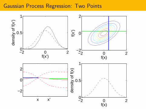
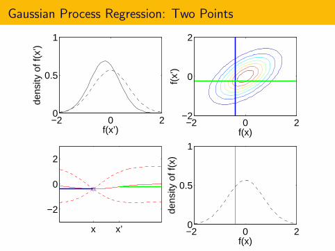
Gaussian Process Regression: Two Points

Fix two points x and x ′.

Consider the values of f at these points, f (x) and f (x ′).

x x’

f(x’)

f(x)

f(x)

f(x’)




x x’

f(x)f(x’)

f(x)

f(x’)




x x’

f(x’)

f(x)

f(x)

f(x’)


f (x) and f (x ′) are unknown before we measure them.

In Bayesian statistics, we model our uncertainty about f with a priorprobability distribution.[

f (x)f (x ′)

]∼ N

([µ0(x)µ0(x ′)

],

[Σ0(x ,x) Σ0(x ,x ′)Σ0(x ′,x) Σ0(x ′,x ′)

])Here, µ0(·) and Σ0(·, ·) are functions to be discussed later.

In general, f (x) and f (x ′) are correlated.


f(x)

f(x’

)

−2 0 2−2

0

2

−2 0 20

0.5

1

f(x)

dens

ity o

f f(x

)

−2 0 20

0.5

1

f(x’)

dens

ity o

f f(x

’)

x x’

−2

0

2

Nearby Points Have Stronger Correlation

The closer x and x ′ are in the feasible domain, the stronger thecorrelation under our belief between f (x) and f (x ′).

f(x)

f(x’

)

−2 0 2−2

0

2

−2 0 20

0.5

1

f(x)

dens

ity o

f f(x

)

−2 0 20

0.5

1

1.5

f(x’)de

nsity

of f

(x’)

x x’

−2

0

2

This should be enforced by our choice of Σ0(·, ·). A common choice isthe power exponential:

Σ0(x ,x ′) = α0 exp(−α1||x−x ′||2

)

Gaussian Process Regression: Two Close Points

f(x)

f(x’

)

−2 0 2−2

0

2

−2 0 20

0.5

1

f(x)

dens

ity o

f f(x

)

−2 0 20

0.5

1

1.5

f(x’)

dens

ity o

f f(x

’)

x x’

−2

0

2

GP Regression: Formal Definition

A GP prior on an unknown function f : Rd 7→ R is parameterized by a

mean function µ0(·).

covariance function Σ0(·, ·), that must be positive semi-definite.

Definition: A prior P on a function f is a Gaussian Process (GP) priorwith mean function µ0 and covariance function Σ0 if:For any given set of points x1, . . . ,xk , under P, f (x1)

...f (xk)

∼ N

µ0(x1)

...µ0(xk)

, Σ0(x1,x1) . . . Σ0(x1,xk)

.... . .

...Σ0(xk ,x1) . . . Σ0(xk ,xk)

The Posterior Can be Computed Analytically

Suppose we have observed

f (~x) = [f (x1), . . . , f (xn)].

Fix any x ′. The posterior on f (x ′) is

f (x ′)|f (~x)∼ N(µn(x ′),σ2n (x ′)).

When µ0(·) = 0, µn(x ′) and σ2n (x ′) are:

µn(x ′) = Σ0(x ′,~x)Σ0(~x ,~x)−1f (~x),

σ2n (x ′) = Σ0(x ′,x ′)−Σ0(x ′,~x ,)Σ0(~x ,~x)−1Σ0(~x ,x ′)

Illustrative 1D Example

50 100 150 200 250 300−2

−1.5

−1

−0.5

0

0.5

1

1.5

2

2.5

x

valu

e

GP Regression and BGO Work in More Than 1 Dimension

For clarity, most of the illustrations in this talk are in 1-dimension.

GP Regression and BGO can also be applied in Rd with d > 1, andalso in combinatorial spaces.

The key is including a notion of distance in Σ0(·, ·), e.g.

Σ0(x ,x ′) = α0 exp(−α1||x−x ′||2

)Mean of Posterior, µn

Bonus 1

Bonu

s 2

0 1 2 30

0.5

1

1.5

2

2.5

3Std. Dev. of Posterior

Bonus 1

Bonu

s 2

0 1 2 30

0.5

1

1.5

2

2.5

3

log(KG Factor)

Bonus 1

Bonu

s 2

0 1 2 30

0.5

1

1.5

2

2.5

3

0 2 4 6 8−2

−1.5

−1

−0.5

0Best Fit

n

log1

0(Be

st F

it)

Outline

1 Introduction





6 Conclusion

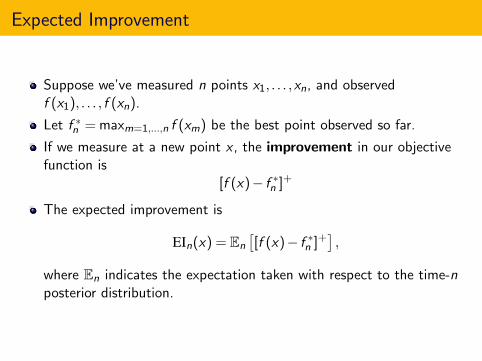
Expected Improvement

In BGO, we use the posterior distribution to decide where to samplenext.

One classic method is called “Efficient Global Optimization” (EGO),and is based on the idea of Expected Improvement.

This method is due to [Jones et al., 1998], building on ideas in[Mockus, 1972].


Suppose we’ve measured n points x1, . . . ,xn, and observedf (x1), . . . , f (xn).

Let f ∗n = maxm=1,...,n f (xm) be the best point observed so far.

If we measure at a new point x , the improvement in our objectivefunction is

[f (x)− f ∗n ]+

The expected improvement is

EIn(x) = En

[[f (x)− f ∗n ]+

],

where En indicates the expectation taken with respect to the time-nposterior distribution.

Expected Improvement Can Be Computed Analytically

Let ∆n(x) = µn(x)− f ∗n be the difference between our estimate off (x) and the best value observed so far. Then,

EIn(x) = En

[[f (x)− f ∗n ]+

]= [∆n(x)]+ + σn(x)ϕ

(∆n(x)

σn(x)

)−|∆n(x)|Φ

(−|∆n(x)|

σn(x)

),

where Φ and ϕ are the normal cdf and pdf,

50 100 150 200 250 300−2

−1

0

1

2

x

valu

e

50 100 150 200 250 3000

0.1

0.2

0.3

0.4

0.5

x

EI


The EGO/EI policy chooses to sample at the point with the largestexpected improvement,

xn+1 = arg maxx

EIn(x)

50 100 150 200 250 300−2

−1

0

1

2

x

valu

e

50 100 150 200 250 3000

0.1

0.2

0.3

0.4

0.5

x

EI



xn+1 = arg maxx

EIn(x)

Each time we decide which point to evaluate next (to solve our overalloptimization problem), we have to solve an optimization problem!

We have replaced one optimization problem (maxx∈A f (x)) with manyoptimization problems (maxx EIn(x), for n = 1,2,3, . . .). Why is this agood thing?

Evaluating f (x) is expensive (minutes, hours, days), and derivativeinformation is unavailable.Evaluating EIn(x) is quick (microseconds), and derivative informationis available.

Maximize Expected Improvement


xn+1 = arg maxx

EIn(x)

One can calculate the gradient of EIn(x) with respect to x .

To solve maxx EIn(x), use a first order method combined withmultistart.

EI Trades Exploration vs. Exploitation

EIn(x) is bigger when µn(x) is bigger.EIn(x) is bigger when σn(x) is bigger.These two tendencies often push against each other, and the EI policymust balance them.

50 100 150 200 250 300−2

−1

0

1

2

x

valu

e

50 100 150 200 250 3000

0.1

0.2

0.3

0.4

0.5

x

EI

EGO Animation

50 100 150 200 250 300−2

−1

0

1

2

x

valu

e

50 100 150 200 250 3000

0.1

0.2

0.3

0.4

0.5

x

EI

Outline

1 Introduction





6 Conclusion

Requirement for Use: Expensive Function Evaluation

BGO is only useful when function evaluation is time-consuming orexpensive.

In the simulation calibration problem discussed later, each functionevaluation takes 3 days.

In the drug development problem discussed later, each functionevaluation takes several days.

How expensive is expensive enough? Function evaluation should takesignificantly longer than the time that the BGO algorithm requires todecide where to sample next.

BGO takes longer to decide where to take each sample, but requiresfewer samples than other methodologies (when it works well).

Requirement for Use: Lack of Gradient Information

If gradient information is available, it is usually better to simply use amultistart first-order method.

Gradient information can be incorporated into a BGO algorithm toimprove its speed, but this is difficult and is not covered here.

Incorporating gradient information into BGO algorithms remains anarea for research.

Other Derivative-Free Global Optimization Methods

Many other derivative-free noise-tolerant global optimization methodsexist, e.g.,

pattern search, e.g., Nelder-Meadstochastic approximation, e.g., SPSA [Spall 1992].evolutionary algorithms, simulated annealing, tabu searchresponse surface methods. [Myers & Montgomery 2002]Lipschitzian optimization, e.g., DIRECT [Gablonsky et al. 2001]

BGO methods require more computation to decide where to evaluatenext, but require fewer evaluations to find global extrema (caveat:when the prior is chosen well).

[Huang et al. 2006] compares sequential kriging optimization (a BGOmethod) against DIRECT 0Gablonsky et al 2001], Nelder-Meadmodified for noise by Humphrey et al 2000, and SPSA [Spall 1992],and finds that SKO requires fewer function evaluations.

BGO is a Surrogate Method

BGO methods operate by maintaining a posterior distribution on theunknown objective function f ,

There is a class of global optimization methods called surrogatemethods that maintain a cheap-to-evaluate approximation to theobjective function, and use this to decide where to sample next. (see,e.g., [Booker et al., 1999, Regis and Shoemaker, 2005])

The mean of the posterior distribution can be thought of as asurrogate, and so, loosely speaking, BGO methods are a type ofsurrogate method.

Outline

1 Introduction





6 Conclusion

Best estimated overall value might be at an unmeasuredpoint

The improvement considered by EI is:

[f (x)− f ∗n ]+ = max(f (x), f ∗n )− f ∗n = f ∗n+1− f ∗n

where f ∗n = maxm≤n f (xm) is the best point we’ve measured by time n.But the point with the best estimated value might not be a pointwe’ve measured.

50 100 150 200 250 300!2

!1.5

!1

!0.5

0

0.5

1

1.5

2

2.5

x

value

50 100 150 200 250 300!2

!1.5

!1

!0.5

0

0.5

1

1.5

2

2.5

x

value

We can measure improvement w.r.t. the best overall value

Replace f ∗n = maxm≤n

f (xm) = maxm≤n

µn(xm) with µ∗n = max

x∈Aµn(x).

50 100 150 200 250 300!2

!1.5

!1

!0.5

0

0.5

1

1.5

2

2.5

x

value

The corresponding improvement is µ∗n+1−µ∗n .

The corresponding value for taking a sample is

En

[µ∗n+1−µ

∗n | xn+1 = x

].

The policy that measures at the x with the largest such value is calledthe knowledge-gradient with correlated beliefs (KGCB) policy.

Knowledge-Gradient with Correlated Beliefs (KGCB)

Call this modified expected improvement the knowledge-gradient(KG) factor

KGn(x) = En

[µ∗n+1−µ

∗n | xn+1 = x

].

The KGCB policy measures at the point with the largest KG factor.

xn+1 ∈ arg maxx

KGn(x).

0 50 100 150 200 250 300!1.5

!1

!0.5

0

0.5

1

1.5

2

x

valu

e

n=4

0 50 100 150 200 250 300!1.5

!1

!0.5

0

0.5

1

1.5

2

x

valu

e

n=5

0 50 100 150 200 250 3000

0.01

0.02

0.03

0.04

x

valu

e

EGO EI

KG factor

0 50 100 150 200 250 3000

0.01

0.02

0.03

0.04

x

valu

e

EGO EI

KG factor

xk, k<n

µx

n

µn

x +/! 2!"n

xx

xk, k<n

µx

n

µn

x +/! 2!"n

xx

0 50 100 150 200 250 300!1.5

!1

!0.5

0

0.5

1

1.5

2

x

va

lue

n=4

0 50 100 150 200 250 300!1.5

!1

!0.5

0

0.5

1

1.5

2

x

va

lue

n=5

0 50 100 150 200 250 3000

0.01

0.02

0.03

0.04

x

va

lue

EGO EI

KG factor

0 50 100 150 200 250 3000

0.01

0.02

0.03

0.04

x

va

lue

EGO EI

KG factor

xk, k<n

µx

n

µn

x +/! 2!"n

xx

xk, k<n

µx

n

µn

x +/! 2!"n

xx

KGCB Requires Fewer Function Evaluations than EGO,but More Computation

0 10 20 30

!4

!3

!2

!1

0

iterations (n)

log 1

0(O

C)

0 10 20 30!0.01

0

0.01

0.02

0.03

iterations (n)

EG

O O

C !

KG

OC

KG

EGO

Graph shows the difference in expected solution quality betweenKGCB and EGO, on noise-free problems.KGCB needs fewer function evaluations to find a good solution, butmore computation to decide where to evaluate.

Outline

1 Introduction





6 Conclusion

Noisy Global Optimization

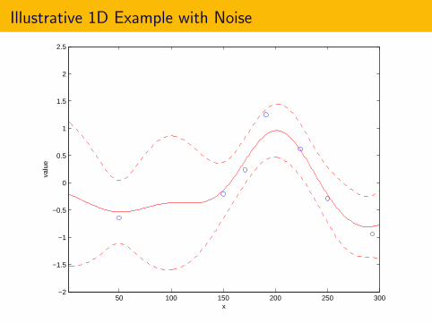
Thus far we have assumed noise-free function evaluations f (x).

What if we observe function evaluations with noise, g(x ,ω)?

We use the same approach:1 Use GP regression to calculate the posterior on f (x) = E[g(x ,ω)] from

noisy function evaluations.2 Use the posterior to decide where to sample next.3 Repeat.

GP Regression Can Be Generalized to Allow Noise

What if we have noisy measurements? i.e., we observeg(x ,ω) = f (x ,ω) + ε(x ,ω).

If the noise is normally distributed with a known (possiblyheterogeneous) variance, then we can still calculate the posterior inessentially the same way.

In practice, the noise is neither normal nor of known variance, but itremains a useful approximation. (In practice, one estimates thevariance as you go.)

Current research examines what can be done to get rid of thisapproximation. (e.g., stochastic kriging from [Ankenman, Nelson andStaum 2010])

Illustrative 1D Example with Noise

50 100 150 200 250 300−2

−1.5

−1

−0.5

0

0.5

1

1.5

2

2.5

x

valu

e

KGCB Can be Generalized to Allow Noise

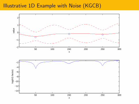
When there is noise, the definition of the KG factor remains the same.

KGn(x) = En

[µ∗n+1−µ

∗n | xn+1 = x

].

The KGCB policy still measures at the point with the largest KGfactor.

xn+1 ∈ arg maxx

KGn(x).

All that changes is that the estimate µn(x) incorporates noise.

50 100 150 200 250 300−2

−1.5

−1

−0.5

0

0.5

1

1.5

2

2.5

x

valu

e

Illustrative 1D Example with Noise (KGCB)

50 100 150 200 250 300−2

−1

0

1

2

x

valu

e

50 100 150 200 250 300

−14

−12

−10

−8

−6

−4

−2

x

log(

KG

fact

or)

There are Many Other BGO Methods

In the interests of time I will not talk about the other BGO methods:[Kushner, 1964, Mockus et al., 1978, Stuckman, 1988, Mockus, 1989,Calvin and Zilinskas, 2002, Calvin and Zilinskas, 2005, Huang et al., 2006,Forrester et al., 2006, Taddy et al., 2009, Villemonteix et al., 2009,Kleijnen et al., 2011],. . .

Outline

1 Introduction





6 Conclusion

Simulation Model Calibration at Schneider National

The logistics company Schneider National uses a largesimulation-based optimization model to try “what if” scenarios.The model has several input parameters that must be tuned to makeits behavior match reality before it can be used.The model is tuned by hand once per year on the most recent data.Each tuning effort requires between 1 and 2 weeks.

© 2008 Warren B. Powell Slide 113

Schneider National

© 2008 Warren B. Powell Slide 114

(Joint work with Warren B. Powell and Hugo Simao, Princeton University,[Frazier et al., 2009a])

Model Parameters

Input parameters to the model include:

time-at-home bonuses.“pacing” parameters describing how fast and far drivers drive per day.gas prices. . .

Output parameters from the model include:

billed milesdriver utilizationaverage number of trips home per driver per 4 weeks.proportion of drivers without time at home over 4 weeks.. . .

Some of these inputs are known (e.g., gas prices), but some areunknown (e.g. time-at-home bonuses).

Goal: adjust the inputs to make the optimal solution found by themodel match current practice.

Simulation Model Calibration

Goal: adjust the inputs to make the optimal solution found by theADP model match current practice.

x is a set of inputs to the simulator.f (x) is how closely the simulator output matches history.

Running the simulator for one set of bonuses takes 3 days, makingcalibration difficult.

The model may be run for shorter periods of time, e.g. 12 hours, toobtain noisy output estimates.

BGO is Flexible Enough to Handle Non-stationary Output

The output of the simulator is non-stationary.

Running the simulator to convergence takes too long (3 days).

With just 12 hours of samples, we can use Bayesian statistics to get anoisy estimate of where the path is going.

0 10 20 30 40 501.4

1.6

1.8

2

2.2

2.4

2.6

2.8

iterations (n)

solo

TA

H

0 50 100 150 2001.8

1.9

2

2.1

2.2

2.3

2.4

2.5

iterations (n)

Est

imat

e of

Gk(ρ

)

Avg of data after n=100

Avg of all data

Posterior mean

Posterion mean ± 2 std dev

Simulation Model Calibration Results

Mean of Posterior, µn

Bonus 1

Bon

us 2

0 1 2 30

0.5

1

1.5

2

2.5

3Std. Dev. of Posterior

Bonus 1

Bon

us 2

0 1 2 30

0.5

1

1.5

2

2.5

3

log(KG Factor)

Bonus 1

Bon

us 2

0 1 2 30

0.5

1

1.5

2

2.5

3

0 2 4 6 8−2

−1.5

−1

−0.5

0Best Fit

n

log1

0(B

est F

it)

Simulation Model Calibration Results

The KG method calibrates the model in approximately 3 days,compared to 7−14 days when tuned by hand.

The calibration is automatic, freeing the human calibrator to do otherwork.

The KG method calibrates as accurately or better than does by-handcalibration.

Current practice uses the year’s calibrated bonuses for each new“what if” scenario, but to enforce the constraint on driver at-hometime it would be better to recalibrate the model for each scenario.Automatic calibration with the KG method makes this feasible.

Outline

1 Introduction





6 Conclusion

Ewings Sarcoma is a Pediatric Bone Cancer

Long-term survival rate is 60−80% for localized disease, and ≈ 20%following metastisis.

Drug Development is Global Optimization

We have a large number of chemically related small molecules, someof which might make a good drug.

We can synthesize and test the quality of these molecules, but eachmolecule tested takes days of effort.

f (x) is the quality of molecule x , and g(x ,ω) is the test result.

We would like to find a good drug with a limited number of tests.

Joint work with Jeffrey Toretsky, M.D. (Georgetown), Diana Negoescu(Stanford), Warren B. Powell (Princeton), [Negoescu et al., 2011])

We Use a Gaussian Process Prior

The molecules we consider share a common skeleton, and aredescribed by which substituents are present at each location. 1

41

4

Jou

rna

l of M

edicin

al C

he

mistry

, 1977, V

ol. 2

0, N

o. 1

1

Ka

tz, Osb

orn

e, Ion

escu

ri

v

m

m

t-

m

m

(9

m

m

*

m

m

m

02

01

ri

m

0

m

0,

o]

co o]

t- o]

(9

o]

Ln

N

e

o]

a

N

o]

ri

N

0

o]

Q,

ri

30

ri

c- ri

(9

m

7..

m

ri

-e

m

3

cv

- d

ri

3

0

ri

Q,

to

t-

(9

LQ

Tr

crj

hl

d

i

d

riri

37

-

ri

ri

ri

Td

--. r(

rid

ri

ri

ri

r-

dri

ri

d

d

v-t

d

3

14

14

Jo

urn

al o

f Med

icina

l Ch

em

istry, 1

977, V

ol. 2

0, N

o. 1

1

Ka

tz, Osb

orn

e, Ion

escu

ri

v

m

m

t-

m

m

(9

m

m

*

m

m

m

02

01

ri

m

0

m

0,

o]

co o]

t- o]

(9

o]

Ln

N

e

o]

a

N

o]

ri

N

0

o]

Q,

ri

30

ri

c- ri

(9

m

7..

m

ri

-e

m

3

cv

- d

ri

3

0

ri

Q,

to

t-

(9

LQ

Tr

crj

hl

d

i

d

riri

37

-

ri

ri

ri

Td

--. r(

rid

ri

ri

ri

r-

dri

ri

d

d

v-t

d

3

We use Gaussian Process regression over the discrete, combinatorial,space of molecules.(over a discrete space, this is also called Bayesian linear regression).

The covariance Σ0(x ,x ′) of two molecules x and x ′ is larger when thetwo molecules have more substituents in common.

This is called the Free-Wilson model in medicinal chemistry [Free andWilson 1964].

KGCB Works Well in TestsCHAPTER 4. IMPLEMENTATION AND PRELIMINARY RESULTS 66

0 10 20 30 40 50 60 70 80 90 1000

0.5

1

1.5

2

2.5

# measurements

max truth ! truth(best µ)

KG

Pure Exploration

Figure 4.13: CKG with Free Wilson model for 99 compounds using the informativeprior and a single truth

compounds almost at random just so that it learns something about their values,

which renders it a not too di!erent policy from Pure Exploration.

Nonetheless, even with the numerical issues coming up in the noninformative

phase, the CKG policy is still doing quite well compared to the other policies, as it

is still the only policy that finds the best compunds in the first 100 measurements.

Informative prior

We have also tested the informative prior for this data set of 99 compounds under

the Free Wilson model, and the resulting plot can be seen in Figure 4.13. Just as

we observed using the 36 compounds data set, the learning rate is again significantly

faster than under the non-informative prior.

Average over 100 sample paths on randomly selected subsets ofbenzomorphan compounds of size 99.

KGCB Works Well in Tests

CHAPTER 5. INCREASING THE NUMBER OF COMPOUNDS 100

0 20 40 60 80 100 120 140 160 180 2000

0.5

1

1.5

2

2.5

3

3.5

4

measurement #

Mean Opportunity Cost (max(truth) ! truth(max belief)) for 25000 compounds

CKG

Pure Exploration

Figure 5.8: Average over nine runs of sample paths using data sets of 25000 com-pounds

0 20 40 60 80 100 120 140 160 180 2000

0.5

1

1.5

2

2.5

3

3.5

4

4.5

5

measurement #

max(truth) ! truth(max belief)

CKG

Pure Exploration

Figure 5.9: A sample path using the entire data set of 87120 compoundsOne sample path on the full set of 87,120 benzomorphan compounds.

Discussion: KGCB Works Well So Far. . .

BGO methods work well in test problems using a chemical datasetfrom the literature. [Negoescu, Frazier, Powell 2011]

Application to Ewing’s sarcoma is ongoing.

Our fingers are crossed. . .

Outline

1 Introduction





6 Conclusion

Details I left out

Choice of prior distribution.

Monitoring the quality of the prior (model validation)

Computational issues

Transforming the objective function to improve model fit

Relationship to kriging

Other BGO methods, [Huang et al., 2006, Taddy et al., 2009,Villemonteix et al., 2009, Kleijnen et al., 2011],. . .

Open problems. . .

Parallelization

Incorporating gradient information

. . .

Software

All software is free unless otherwise noted.

http://optimallearning.princeton.edu/ and go to “DownloadableSoftware”

TOMLAB (http://tomopt.com/tomlab/) a (commercial) Matlabadd-on with implementations noise-free EGO on continuous spaces.

SPACE (http://www.schonlau.net/space.html), an implementation ofEGO in C on continuous spaces.

the matlabKG library(http://people.orie.cornell.edu/pfrazier/src.html) an implementationof the KGCB algorithm for noisy discrete problems. I am planning toimprove this library, both with respect to speed and usability — if youuse it, please send me an email and share your experiences.

Software library accompanying the book by Sobester & Keane, Go tohttp://www.soton.ac.uk/˜aijf197/ and search for “software”.

http://optimallearning.princeton.edu/

http://tomopt.com/tomlab/

http://www.schonlau.net/space.html

http://people.orie.cornell.edu/pfrazier/src.html

http://www.soton.ac.uk/~aijf197/

More Software

dace, a matlab kriging toolboxhttp://www2.imm.dtu.dk/˜hbn/dace/. A Matlab library for doingkriging, which is very similar to GP regression. Assumes noise-freefunction evaluations, but can be easily tweaked.

stochastic kriging, http://stochastickriging.net/. Matlab code forobtaining kriging estimates with unknown and variable sampling noise.

For other GP regression software from the machine learningcommunity, see http://www.gaussianprocess.org.

http://www2.imm.dtu.dk/~hbn/dace/

http://stochastickriging.net/

http://www.gaussianprocess.org

Introductory Reading

Brochu, E., Cora, V. M., and de Freitas, N. (2009).

A tutorial on Bayesian optimization of expensive cost functions, withapplication to active user modeling and hierarchical reinforcement learning.

Technical Report TR-2009-23, Department of Computer Science, Universityof British Columbia.

Forrester, A., Sobester, A., and Keane, A. (2008).

Engineering design via surrogate modelling: a practical guide.

Wiley, West Sussex, UK.

Powell, W. and Frazier, P. (2008).

Optimal Learning.

TutORials in Operations Research: State-of-the-Art Decision-Making Toolsin the Information-Intensive Age, pages 213–246.

Rasmussen, C. and Williams, C. (2006).

Gaussian Processes for Machine Learning.

MIT Press, Cambridge, MA.

Introductory and Advanced Reading (added after talk)

Warren Powell and Ilya Ryzhov have a book called “OptimalLearning” that will be published in 2012.

Some introductory (and advanced) material may be found athttp://optimallearning.princeton.edu/

(advanced reading) The KGCB algorithm for discrete and continuousspaces is introduced in [Frazier et al., 2009b, Scott et al., 2011].

Advanced surveys and research papers may be found athttp://people.orie.cornell.edu/pfrazier/

http://optimallearning.princeton.edu/

http://people.orie.cornell.edu/pfrazier/

Conclusion

BGO methods use the Bayesian posterior on the unknown function todecide where to sample next.

They tend to require a lot of computation to decide where to sample,but reduce the overall number of samples required.

They are very flexible, and the Bayesian statistical used can be tunedto new applications (non-stationary output, combinatorial feasible set,. . . )

Thank You

Any questions?

Choice of µ0(·)

The Gaussian process prior is parameterized by µ0(·) and Σ0(·, ·).

How should we choose these functions?

One common choice for µ0(·) is simply to set it to a constant β0.

Typically, one estimates this constant adaptively using maximumlikelihood. (Discussed later)Alternatively, if one places an independent normal prior on β0, then thiscan be folded back into the GP prior.Coupled with typical choices for Σ(·, ·), this produces a prior that isstationary across the domain: for any a, the likelihood that f (x) = adoes not depend on x .

Choice of µ0(·)

Alternatively, if we suspect strong trends in f , we can choose acollection of basis functions φ1, . . . ,φK , and set

µ0(x) = β0 + β1φ1(x) + · · ·+ βKφm(x).

This generally does not produce a stationary prior.Typically one estimates β0, . . . ,βm using maximum likelihood.Alternatively, one can place normal priors on the βk .

Choice of Σ0(·)We usually choose Σ0(·, ·) from one of a few parametric classes ofcovariance functions.

isometric Gaussian

Σ0(x ,x ′) = α0 exp(−α1||x−x ′||22

)power exponential

Σ0(x ,x ′) = α0 exp

(−

D

∑d=1

αd |ed · (x−x ′)|p)

For others, see [Cressie, 1993, Rasmussen and Williams, 2006].

By choosing different parameter values, we can encode different beliefs inthe smoothness of f .

0 50 100−3

−2

−1

0

1

2

3

0 50 100−4

−3

−2

−1

0

1

2

0 50 100−2

−1

0

1

2

3

We estimate these parameters adaptively using maximum likelihood.

Empirical Bayes Estimation of Parameters

We have observed x1, . . . ,xn, and y1 = f (x1), . . . ,yn = f (xn).

We have a Gaussian process prior with µ(·), Σ(·, ·).

µ(·) and Σ(·, ·) are parameterized in turn by a collection ofparameters ν .

To estimate ν , we calculate the density of the prior at the observeddata,

P(y1, . . . ,yn;ν)

This density is multivariate normal with a mean and covariance thatdepends on ν .

We find the ν that maximizes this density, and this is our estimate.

ν ∈ arg maxν

P(y1, . . . ,yn;ν)

We generally update this estimate as we obtain more data.

References I

Booker, A., Dennis, J., Frank, P., Serafini, D., Torczon, V., and Trosset, M. (1999).

A rigorous framework for optimization of expensive functions by surrogates.Structural and Multidisciplinary Optimization, 17(1):1–13.

Brochu, E., Cora, V. M., and de Freitas, N. (2009).

A tutorial on Bayesian optimization of expensive cost functions, with application to active user modeling and hierarchicalreinforcement learning.Technical Report TR-2009-23, Department of Computer Science, University of British Columbia.

Calvin, J. and Zilinskas, A. (2002).

One-dimensional Global Optimization Based on Statistical Models.Nonconvex Optimization and its Applications, 59:49–64.

Calvin, J. and Zilinskas, A. (2005).

One-Dimensional global optimization for observations with noise.Computers & Mathematics with Applications, 50(1-2):157–169.

Cressie, N. (1993).

Statistics for Spatial Data, revised edition.Wiley Series in Probability and Mathematical Statistics: Applied Probability and Statistics. Wiley Interscience, New York.

Forrester, A., Keane, A., and Bressloff, N. (2006).

Design and Analysis of” Noisy” Computer Experiments.AIAA Journal, 44(10):2331–2339.

Forrester, A., Sobester, A., and Keane, A. (2008).

Engineering design via surrogate modelling: a practical guide.Wiley, West Sussex, UK.

References II

Frazier, P., Powell, W., and Simao, H. (2009a).

Simulation model calibration with correlated knowledge-gradients.In Winter Simulation Conference Proceedings, 2009. Winter Simulation Conference.

Frazier, P., Powell, W. B., and Dayanik, S. (2009b).

The knowledge gradient policy for correlated normal beliefs.INFORMS Journal on Computing, 21(4):599–613.

Huang, D., Allen, T., Notz, W., and Miller, R. (2006).

Sequential kriging optimization using multiple-fidelity evaluations.Structural and Multidisciplinary Optimization, 32(5):369–382.

Jones, D., Schonlau, M., and Welch, W. (1998).

Efficient Global Optimization of Expensive Black-Box Functions.Journal of Global Optimization, 13(4):455–492.

Kleijnen, J., van Beers, W., and van Nieuwenhuyse I. (2011).

Expected improvement in efficient global optimization through bootstrapped kriging.Journal of Global Optimization, pages 1–15.

Kushner, H. J. (1964).

A new method of locating the maximum of an arbitrary multi- peak curve in the presence of noise.Journal of Basic Engineering, 86:97–106.

Mockus, J. (1972).

On bayesian methods for seeking the extremum.Automatics and Computers (Avtomatika i Vychislitelnayya Tekchnika), 4(1):53–62.(in Russian).

References III

Mockus, J. (1989).

Bayesian approach to global optimization: theory and applications.Kluwer Academic, Dordrecht.

Mockus, J., Tiesis, V., and Zilinskas, A. (1978).

The application of Bayesian methods for seeking the extremum.In Dixon, L. and Szego, G., editors, Towards Global Optimisation, volume 2, pages 117–129. Elsevier Science Ltd., NorthHolland, Amsterdam.

Negoescu, D., Frazier, P., and Powell, W. (2011).

The knowledge gradient algorithm for sequencing experiments in drug discovery.INFORMS Journal on Computing, 23(1).

Powell, W. and Frazier, P. (2008).

Optimal Learning.TutORials in Operations Research: State-of-the-Art Decision-Making Tools in the Information-Intensive Age, pages213–246.

Rasmussen, C. and Williams, C. (2006).

Gaussian Processes for Machine Learning.MIT Press, Cambridge, MA.

Regis, R. and Shoemaker, C. (2005).

Constrained Global Optimization of Expensive Black Box Functions Using Radial Basis Functions.Journal of Global Optimization, 31(1):153–171.

Scott, W., Frazier, P. I., and Powell, W. B. (2011).

The correlated knowledge gradient for simulation optimization of continuous parameters using gaussian processregression.SIAM Journal on Optimization, 21:996–1026.

References IV

Stuckman, B. (1988).

A global search method for optimizing nonlinear systems.Systems, Man and Cybernetics, IEEE Transactions on, 18(6):965–977.

Taddy, M., Lee, H., Gray, G., and Griffin, J. (2009).

Bayesian guided pattern search for robust local optimization.Technometrics, 51(4):389–401.

Villemonteix, J., Vazquez, E., and Walter, E. (2009).

An informational approach to the global optimization of expensive-to-evaluate functions.Journal of Global Optimization, 44(4):509–534.

Yang, W., Feinstein, J., and Marsden, A. (2010).

Constrained optimization of an idealized y-shaped baffle for the fontan surgery at rest and exercise.Computer methods in applied mechanics and engineering, 199(33-36):2135–2149.


EIn(x) = [∆n(x)]+ + σn(x)ϕ

(∆n(x)σn(x)

)−|∆n(x)|Φ

(− |∆n(x)|

σn(x)

)EIn(x) is determined by ∆n(x) = µn(x)− f ∗n and σn(x).

EIn(x) increases as ∆n(x) increases.

Measure where f (x) seems large. (Exploitation)

EIn(x) increases as σn(x) increases.

Measure where we are uncertain about f (x). (Exploration)


EIn(x) is bigger when µn(x) is bigger.EIn(x) is bigger when σn(x) is bigger.Below is a contour plot of EIn(x). Red is bigger EI.

σn(x)

∆ n(x)

0.2 0.4 0.6 0.8 1−1

−0.5

0

0.5

1

Knowledge-Gradient with Correlated Beliefs (KGCB)

Call this modified expected improvement the knowledge-gradient(KG) factor

KGn(x) = En

[µ∗n+1−µ

∗n | xn+1 = x

].

The KGCB policy measures at the point with the largest KG factor.

xn+1 ∈ arg maxx

KGn(x).

0 50 100 150 200 250 300!1.5

!1

!0.5

0

0.5

1

1.5

2

x

valu

e

n=4

0 50 100 150 200 250 300!1.5

!1

!0.5

0

0.5

1

1.5

2

x

valu

e

n=5

0 50 100 150 200 250 3000

0.01

0.02

0.03

0.04

x

valu

e

EGO EI

KG factor

0 50 100 150 200 250 3000

0.01

0.02

0.03

0.04

x

valu

e

EGO EI

KG factor

xk, k<n

µx

n

µn

x +/! 2!"n

xx

xk, k<n

µx

n

µn

x +/! 2!"n

xx

0 50 100 150 200 250 300!1.5

!1

!0.5

0

0.5

1

1.5

2

x

va

lue

n=4

0 50 100 150 200 250 300!1.5

!1

!0.5

0

0.5

1

1.5

2

x

va

lue

n=5

0 50 100 150 200 250 3000

0.01

0.02

0.03

0.04

x

va

lue

EGO EI

KG factor

0 50 100 150 200 250 3000

0.01

0.02

0.03

0.04

x

va

lue

EGO EI

KG factor

xk, k<n

µx

n

µn

x +/! 2!"n

xx

xk, k<n

µx

n

µn

x +/! 2!"n

xx

tutorial: bayesian methods for global and simulation ... bayesian methods for global and simulation...

Documents