tutorial: automatic diﬀerentiation with openad ... · dagstuhl feb 2009 tutorial: ... tutorial:...

Dagstuhl Feb 2009 Tutorial: OpenAD & combinatorial problems 1'

&

$

%

Tutorial: Automatic differentiation

with OpenAD & combinatorial

problems

Jean Utke

• things to consider when choosing AD tools & methods

• OpenAD basic use

• reversal schemes

• computational graphs

• nonsmooth behavior

• writing models with AD in mind...

Utke Argonne


&

$

%

contributions to the OpenAD source code

Naumann

Norris

Tallent

Fagan

Strout

Gottschling

Lyons

summer students,...

numerous non-code contributions by Hovland, Hascoet, ...

Utke Argonne


&

$

%

what to pick...

i.e. matching application requirements with AD tools and techniques

the major advantages of AD are ... no need to repeat again

• knowing AD tool “internal” algorithms is of interest to the user

(compare to compiler vector optimization)

• except for simple models and low computational complexity

→ can get away with “something”

• complicated models → worry about tool applicability

• high computational complexity → worry about efficiency of derivative

computations

• tool availability (e.g. source transformation for C++ ?)

Utke Argonne


&

$

%

Source Transformation vs. Operator Overloading

• complicated implementation of tools

• especially for reverse mode

• full front end, back end, analysis

• efficiency gains from

– compile time optimizations

– activity analysis

– explicit control flow reversal for reverse

mode

• source transformation based type change &

overloaded operators appropriate for

higher-order derivatives.

• benefits from external information

• efficiency depends on analysis accuracy

• simple tool implementation

• reverse mode (generating and reinterpreting

an execution trace → inefficient)

• implemented as some library

• impact on efficiency:

– library implementation (narrow scope)

– compiler inlining capabilities (for low

order)

– use external information (sparsity etc.)

– can do only runtime optimizations

• manual type change for operator overloading

– complicated for formatted I/O,

allocation

– need matching signatures in Fortran

– helped by use of templates

For higher-order derivatives combining source transformation based type

change with overloaded operators is appropriate.

Utke Argonne


&

$

%

Forward vs. Reverse

• simplest rule: given y = f(x) : IRn 7→ IRm use reverse if n ≫ m (gradient)

• what if n ≈ m and large

– want only projections, e.g. Jx

– sparsity (e.g. of the Jacobian)

– partial separability (e.g. f(x) =∑

(fi(xi)), xi ∈ Di ⋐ D ∋ x)

– intermediate interfaces of different size

• the above may make forward mode feasible (projection yT J requires

reverse)

• higher order tensors (practically feasible for small n) → forward mode

(reverse mode saves factor n in effort only once)

• this determines overall propagation direction, not necessarily the local

preaccumulation (combinatorial problem)

Utke Argonne


&

$

%

OpenAD overview

• www.mcs.anl.gov/OpenAD

• forward and reverse

• source transformation

• modular design

• large problems

• language independent transformation

• researching combinatorial problems

• current Fortran front-end Open64

(Open64/SL branch at Rice U)

• migration to Rose (already used for

C/C++ with EDG)

• Rapsodia for higher-order derivatives

via type change transformation

• uses association by address as opposed

to association by name

OpenAnalysis

whirl

SageToXAIF

xercesboostAngel

Sage3EDG/front − ends

XAIF

(AD source transformation)xaifBooster

FortTkOpen

Open64

AD/

Fortran pipeline:

whirl2xaif xaif2whirl

F’

whirlF’

xaifxaifF

Fwhirl

F

xaifBooster

F’

OpenAnalysis

Open64

Utke Argonne


&

$

%

toy example

subroutine head(x,y)

double precision,intent(in) :: x

double precision,intent(out) :: y

!$openad INDEPENDENT(x)

y=sin(x*x)

!$openad DEPENDENT(y)

end subroutine

result of pushing it through the pipeline →

program driver

use OAD_active

implicit none

external head

type(active):: x, y

x%v=.5D0

x%d=1.0

call head(x,y)

print *, "F(1,1)=",y%d

end program driver

SUBROUTINE head(X, Y)

use w2f__types

use OAD_active

IMPLICIT NONE

REAL(w2f__8) OpenAD_Symbol_0

...

REAL(w2f__8) OpenAD_Symbol_5

type(active) :: X

INTENT(IN) X

type(active) :: Y

INTENT(OUT) Y

OpenAD_Symbol_0 = (X%v*X%v)

Y%v = SIN(OpenAD_Symbol_0)

OpenAD_Symbol_2 = X%v

OpenAD_Symbol_3 = X%v

OpenAD_Symbol_1 = COS(OpenAD_Symbol_0)

OpenAD_Symbol_5 = ((OpenAD_Symbol_3 +

OpenAD_Symbol_2) * OpenAD_Symbol_1)

CALL sax(OpenAD_Symbol_5,X,Y)

RETURN

END SUBROUTINE

Utke Argonne


&

$

%

scripted pipeline

openad is Python script to invoke pipeline components for simple(!) settings

Usage:~> openad -h

Usage: openad [options] <fortran-file>

Options:

-h, --help show this help message and exit

-m MODE, --mode=MODE basic transformation mode with MODE being one of: rs =

reverse split; t = tracing; rj = reverse joint; f =

forward;

-d DEBUG, --debug=DEBUG

the debugging level

-i, --interactive requires to confirm each command

-k, --keepGoing keep going despite errors

-c, --copy copy run time support files instead of linking them

-n, --noAction display the pipeline commands, do not run them

progress messages:~> openad -c -m f head.prepped.f90

openad log: openad.2009-01-27_14:21:07.log~

parsing head.prepped.f90

analyzing source code and translating to xaif

tangent linear transformation

getting runtime support file OAD_active.f90

getting runtime support file w2f__types.f90

getting runtime support file iaddr.c

translating transformed xaif to whirl

unparsing transformed whirl to fortran

postprocessing transformed fortran

⇒ run the example

on the laptop and

look at the transfor-

mation stages...

Utke Argonne


&

$

%

~> openad -n -c -m f head.prepped.f90

# parsing head.prepped.f90

${OPENADROOT}/Open64/osprey1.0/targ_ia32_ia64_linux/crayf90/sgi/mfef90 -z -F -N132 head.prepped.f90

# analyzing source code and translating to xaif

${OPENADROOT}/OpenADFortTk/OpenADFortTk-x86-Linux/bin/whirl2xaif -n -o head.prepped.xaif head.prepped.B

# tangent linear transformation

${OPENADROOT}/xaifBooster/../xaifBooster/algorithms/BasicBlockPreaccumulation/driver/oadDriver \\

-c ${OPENADROOT}/xaif/schema/examples/inlinable_intrinsics.xaif \\

-s ${OPENADROOT}/xaif/schema -i head.prepped.xaif -o head.prepped.xb.xaif

# getting runtime support file OAD_active.f90

cp -f ${OPENADROOT}/runTimeSupport/scalar/OAD_active.f90 ./

# getting runtime support file w2f__types.f90

cp -f ${OPENADROOT}/runTimeSupport/all/w2f__types.f90 ./

# getting runtime support file iaddr.c

cp -f ${OPENADROOT}/runTimeSupport/all/iaddr.c ./

# translating transformed xaif to whirl

${OPENADROOT}/OpenADFortTk/OpenADFortTk-x86-Linux/bin/xaif2whirl --structured head.prepped.B head.prepped.xb.xaif

# unparsing transformed whirl to fortran

${OPENADROOT}/Open64/osprey1.0/targ_ia32_ia64_linux/whirl2f/whirl2f -openad head.prepped.xb.x2w.B

# postprocessing transformed fortran

perl ${OPENADROOT}/OpenADFortTk/OpenADFortTk-x86-Linux/bin/multi-pp.pl -f head.prepped.xb.x2w.w2f.f

whirl2xaif xaif2whirl

F’

whirlF’

xaifxaifF

Fwhirl

F

xaifBooster

F’

OpenAnalysis

Open64

Utke Argonne


&

$

%

the same example in mode example

script invoked with a different flag

∼> openad -c -m rj head.prepped.f90

program driver

use OAD_active

use OAD_rev

implicit none

external head

type(active) :: x, y

x%v=.5D0

y%d=1.0D0

our_rev_mode%tape=.TRUE.

call head(x,y)

print *, ’driver running for x =’,x%v

print *, ’ yields y =’,y%v,’ dy/dx =’,x%d

print *, ’ 1+tan(x)^2-dy/dx =’,1.0D0+tan(x%v)**2-x%d

end program driver

~> openad -c -m rj head.prepped.f90

openad log: openad.2009-01-28_13:16:59.log~

parsing head.prepped.f90

analyzing source code and translating to xaif

adjoint transformation

getting runtime support file OAD_active.f90

getting runtime support file w2f__types.f90

getting runtime support file iaddr.c

getting runtime support file ad_inline.f

getting runtime support file OAD_cp.f90

getting runtime support file OAD_rev.f90

getting runtime support file OAD_tape.f90

getting template file

translating transformed xaif to whirl

unparsing transformed whirl to fortran

postprocessing transformed fortran

note: -m rj means reverse joint mode; needs extra run time support files

OAD cp/rev/tape; modified driver makes reference to the reversal scheme

(checkpointing)

... need to talk about taping and checkpointing.

Utke Argonne


&

$

%

Reversal / Checkpointing Schemes

• why it is needed

• major modes

• OpenAD implementation

• alternatives

Utke Argonne


&

$

%

recap - why we need a tape...

f : y = sin(a ∗ b) ∗ c

yields a graph representing the order of computation:

b a

cos(t1)

c

*

*

a b c

t1

t2

t2

sin

• intrinsics φ(. . . , w, . . .) have local partial derivatives∂φ∂w

• e.g. sin(t1) yields cos(t1)

• code list→ intermediate values t1 and t2

• all others already stored in variables

t1 = a*b

p1 = cos(t1)

t2 = sin(t1)

y = t2*c

What can we do with this?

Utke Argonne


&

$

%

reverse with adjoints

Assume variable and adjoints associated in pairs (v,g v):

b a

c

*

*

a b c

t1

t2

t2

sin

g_y

p1

append computations of adjoints

t1 = a*b

p1 = cos(t1)

t2 = sin(t1)

y = t2*c

g_c = g_y*t2

g_t2 = g_y*c

g_t1 = g_t2*p1

g_b = g_t1*a

g_a = g_t1*b

require p1 in the adjoint sweep ⇒ recompute (time) or store (taping space)

Utke Argonne


&

$

%

may also need control flow trace and addresses...

original CFG ⇒ record a path through the CFG ⇒ adjoint CFG

Entry(1)

B(2)

Branch(3)

B(4)

T

Loop(5)

F

EndBranch(8)

B(9)

Exit(10)

F

B(6)

T

EndLoop(7)

⇒

Entry(1)

B(2)’

Branch(3)

B(4)’

T

iLc

F

pB T

EndBranch(8)

B(9)’

Exit(10)

Loop(5)

B(6)’

T

pLc

F

+Lc

EndLoop(7)

pB F

⇒

Entry(10)

B(9)’’

pB

Branch(8)

B(4)’’

T

pLc

F

Loop(7)

B(6)’’

T

EndBranch(3)

F

EndLoop(5)B(2)’’

Exit(1)

often cheap with structured control flow and simple address computations (e.g.

index from loop variables)

unstructured control flow and pointers are expensive

Utke Argonne


&

$

%

trace all at once = global split mode

subroutine 1

call 2; ...

call 4; ...

call 2;

end subroutine 1

subroutine 2

call 3

end subroutine 2

subroutine 4

call 5

end subroutine 4

11

31 3251

4121 22

11 11

3131 3232 5151

41 41 2121 2222

Snn-th invocation of subroutine S run forward and tape

subroutine call run adjoint

order of execution store checkpoint

run forward restore checkpoint

• have memory limits - need to create tapes for short sections in reverse order

• subroutine is “natural” checkpoint granularity, different mode...

Utke Argonne


&

$

%

trace one SR at a time = global joint mode

11 11

31313131 32323232 51515151

414141 212121 222222

taping-adjoint pairs

checkpoint-recompute pairs

the deeper the call stack - the more recomputations (unimplemented solution -

result checkpointing)

familiar tradeoff between storing and recomputation at a higher level but in

theory can be all unified.

Utke Argonne


&

$

%

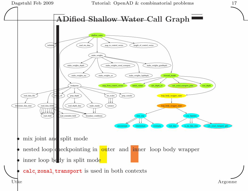
ADified Shallow Water Call Graph

inifields

readparms

read_data_file

read_data_fields

prep_depthcheck_cfl

make_masks

ini_scales prep_coriolis

determine_data_time

read_field read_extended_field boundary_conditions

read_depth_data variance

map_from_control_vector

loop_body_wrapper_outer

read_data

read_eta_data

make_weights

is_eta_data_time

make_weights_depth

make_weights_eta make_weights_uv

make_weights_zonal_transport

make_weights_lapldepth

make_weights_graddepth

forward_model

map_to_control_vector length_of_control_vector

time_step

umomentum vmomentum continuity calc_zonal_transport_split

initial_values calc_depth_uv calc_zonal_transport_joint

cost_function

cost_depth

loop_body_wrapper_inner

shallow_water

• mix joint and split mode

• nested loop checkpointing in outer and inner loop body wrapper

• inner loop body in split mode

• calc zonal transport is used in both contexts

Utke Argonne


&

$

%

OpenAD reversal modes with checkpointing

subroutine level granularity

f

i1 i2 i3 i4

o1 o2

f

o2 o2

i4 i4 i4i3

plain mode

i3 i3

split mode

Utke Argonne


&

$

%

in OpenAD orchestrated with templates

• OpenAnalysis provides side-effect analysis

• provides checkpoint sets as (formal) arguments & references to global variables

• we ask for four sets: ModLocal ⊆ Mod, ReadLocal ⊆ Read

S

S1

2

template variablessubroutine variablessetup

state indicates task 1

pre state chng. task 1

post state chng. task 1

state indicates task 2

pre state chng. task 2

post state chng. task 2

wrapup

subroutine template()

use OAD_tape ! tape storage

use OAD_rev ! state structure

!$TEMPLATE_PRAGMA_DECLARATIONS

if (rev_modetape) then

! the state component

! ’taping’ is true

!$PLACEHOLDER_PRAGMA$ id=2

end if

if (rev_modeadjoint) then

! the state component

! ’adjoint’ run is true

!$PLACEHOLDER_PRAGMA$ id=3

end if

end subroutine template

⇒ run the simple exam-

ple on the laptop with -m

rs and -m rj and look at

the output;

⇒ look at the Shal-

lowWater example.

Utke Argonne


&

$

%

replacing hard wired logic with revolve

• loop extracted into subroutine...

• use revolve to control the behavior

• mercurial repository of a F9X implementation at

http://mercurial.mcs.anl.gov/ad/RevolveF9X

Utke Argonne


&

$

%

User view on checkpointing

have model with high computational complexity and need adjoints

• have model with high computational complexity and need adjoints

• spatial requirements (NP complete DAG/call tree reversal)

• in theory: no distinction between checkpoints and trace

• limited automatic support

• in practice: well defined location for argument checkpoints

– fix checkpoint location and spacing (trace fits into memory)

– tool determines checkpoint elements

– use hierarchical checkpointing (to limit number of checkpoints)

• optimize scheme e.g. with revolve (uniform steps)

but I want to try something else with this..., for instance

Utke Argonne


&

$

%

general reversal example

1111

212121 2222 23 23

313131 3232

414141

• we have 4 tape units

• 22 and23 behave like split, 21 behaves like joint

• How do we control the behavior?

• runtime estimates for checkpoint/tape size and recomputation effort → derive

reversal scheme according to memory/runtime limits as dynamic call tree

Utke Argonne


&

$

%

runtime profiles...

box_model_body 0:3752 0:0:0

box_final_state 0:2 6:0:0

1

box_forward 0:4 41:1:0

3650

box_ini_fields 12:63 20:0:0

1

box_cycle_fields 0:25 12:0:0

3650

box_robert_filter 12:25 10:0:0

7300

box_timestep 11:1 19:0:0

7300

box_transport 3:0 5:0:0

3650

box_density 6:13 8:0:0

3650

box_update 6:13 7:0:0

7300

SubroutineName tape double:integer checkpoint double:integer:boolean

• data “visibility” and upon forced inclusion in the scope name clashes...?

• experimenting with different checkpoint sets

(OpenAnalysis supplies: REF vs.LREF vs. MOD vs. LMOD etc. and these \ {local vars})

• experimenting with result checkpoints...

Utke Argonne


&

$

%

checkpoint sets...

• always Readcallee ⊆ Readcaller

• multiple writes of x /∈ ReadLocal

• can store only x ∈ ReadLocal (except in callers whose callees don’t store anything)

1

4

2

3

4 4

2

3

2

3 3

4

1

4

(s, t, r)

(t, r)

(r)

1

4

2

3

4 4

2

3

2

3 3

4

1

4

(s, t, r)

(t, r)

(r)

s

t

r

(r is ’big’)

• loose stack format; same storage requirements;

• same number of (’big’) reads; fewer ’big’ writes.

• to experiment with this use different versions of store/restores in the template...

Utke Argonne


&

$

%

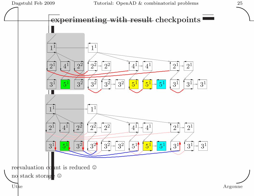
experimenting with result checkpointsreplacemen

11 11

31313131 32323232 51515151

414141 212121 222222

11 11

31313131 32323232 51515151

414141 212121 222222

reevaluation count is reduced ,

no stack storage /

Utke Argonne


&

$

%

... one more call layer

1111

21 2121

313131 31

41 42 41414141 42 424242

• a more suitable storage format is the dynamic call tree

• sample DCT generator can be found in the OpenAD run time support

and now for something completely different...

Utke Argonne


&

$

%

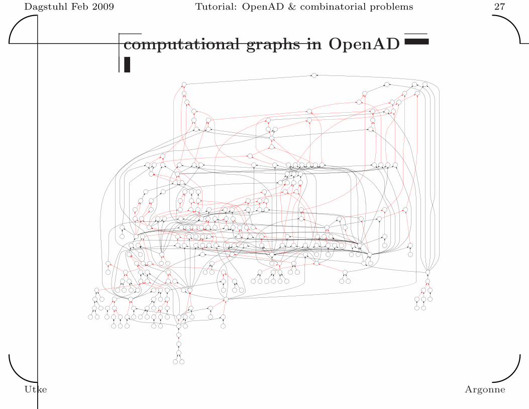
computational graphs in OpenAD

Utke Argonne


&

$

%

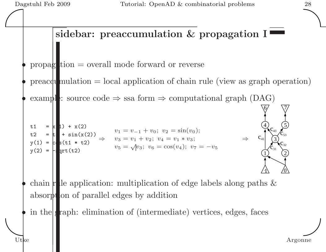
sidebar: preaccumulation & propagation I

• propagation = overall mode forward or reverse

• preaccumulation = local application of chain rule (view as graph operation)

• example: source code ⇒ ssa form ⇒ computational graph (DAG)

t1 = x(1) + x(2)

t2 = t1 + sin(x(2))

y(1) = cos(t1 * t2)

y(2) = -sqrt(t2)

⇒v1 = v−1 + v0; v2 = sin(v0);

v3 = v1 + v2; v4 = v1 ∗ v3;

v5 =√

v3; v6 = cos(v4); v7 = −v5

⇒ 41cc53

c32c31

43c

0

21

3

54

6 7

1−

• chain rule application: multiplication of edge labels along paths &

absorption of parallel edges by addition

• in the graph: elimination of (intermediate) vertices, edges, faces

Utke Argonne


&

$

%

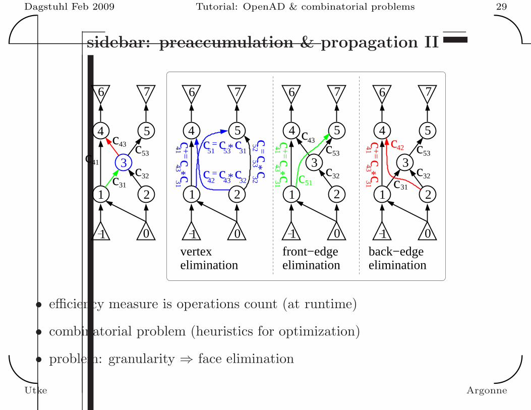
sidebar: preaccumulation & propagation II

c32

c+

=c

41

*c43

31

c+

=c

41

*c43

31

c+

=c

41

*c43

3141c 53

c3231

c53 c53

c32

43c

0

2

3

54

6 7

1−

6 7 6 7 6

4 5 4 5

1 2 1 2

1− 0 1− 0

7

54

33

1 2

0−

31c

c43

1

c c42

c51

43c c

32

31c*

*

c53 c

* c32

5352

c=

=

=

51c

c c42

1

elimination elimination eliminationvertex front−edge back−edge

• efficiency measure is operations count (at runtime)

• combinatorial problem (heuristics for optimization)

• problem: granularity ⇒ face elimination

Utke Argonne


&

$

%

sidebar: preaccumulation & propagation III

1− 1− 1−

4

3

21

5

41

c31

7

c 41c

0 0

21

3

54

6 7 6 7

54

3

21

0

6

c43

c41 +

=c43 c

31

*c

c43

31c

43

31

c

• granularity is single fused multiply add

• also requires heuristics

• elimination sequence terminates with tripartite dual graph, i.e. Jacobian

Utke Argonne


&

$

%

sidebar: preaccumulation & propagation IV

have preaccumulated local Jacobians;

given the J i, i = 1, . . . , k we want to do:

• forward: (Jk ◦ . . . ◦ (J1 ◦ x) . . .), or

• reverse: (. . . (yT ◦ Jk) ◦ . . . ◦ J1)

the total cost:

• function evaluation + local partials (fixed)

• preaccumulation (NP-hard, varying with heuristic)

• propagation (fixed for a given preaccumulation)

– for simplicity: one saxpy per non-unit J i element

– potential for n-ary saxpys (generated)

What – other than the preaccumulation heuristic - can vary?

Utke Argonne


&

$

%

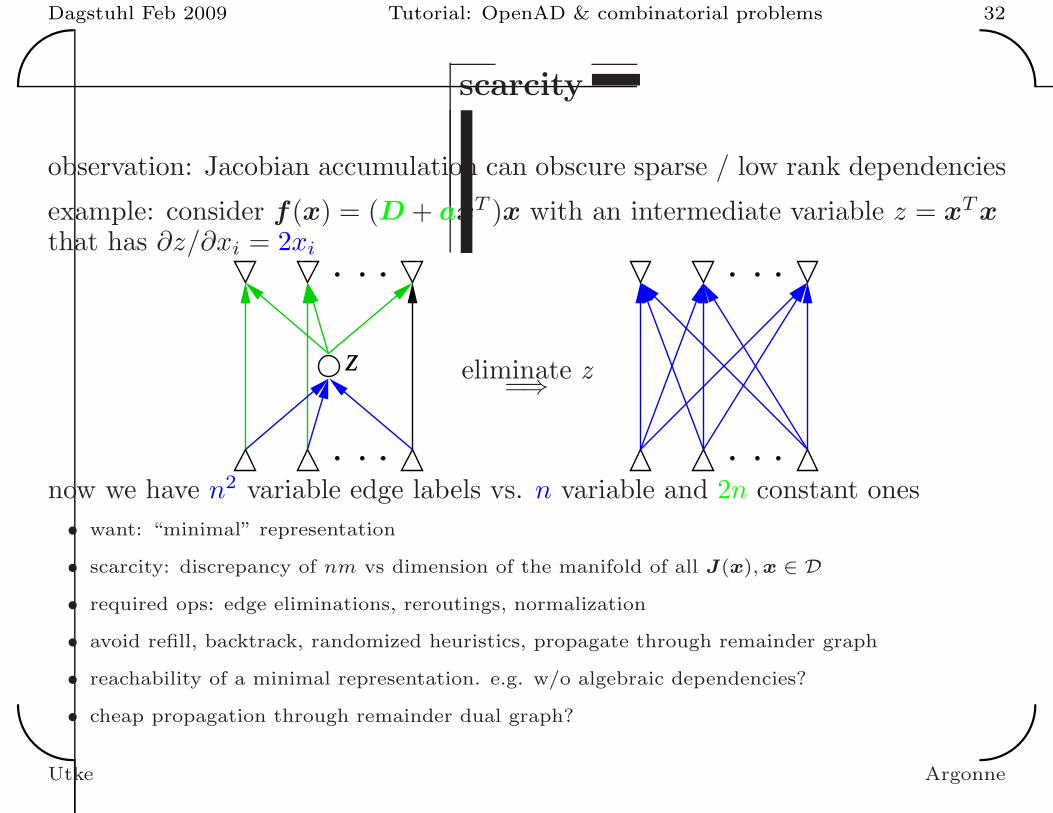
scarcity

observation: Jacobian accumulation can obscure sparse / low rank dependencies

example: consider f(x) = (D + axT )x with an intermediate variable z = xT xthat has ∂z/∂xi = 2xi

z eliminate z=⇒

now we have n2 variable edge labels vs. n variable and 2n constant ones

• want: “minimal” representation

• scarcity: discrepancy of nm vs dimension of the manifold of all J(x), x ∈ D

• required ops: edge eliminations, reroutings, normalization

• avoid refill, backtrack, randomized heuristics, propagate through remainder graph

• reachability of a minimal representation. e.g. w/o algebraic dependencies?

• cheap propagation through remainder dual graph?

Utke Argonne


&

$

%

example

DAG with unit/constant edges

HEX86aea20

FLUX1_20 k=2 d

HEX8744238

FLUX2_21 k=2 d

HEX8746d18

FLUX3_22 k=2 d

HEX874af40

FLUX4_23 k=2 d

HEX874f100

FLUX5_24 k=2 d

HEX87532c0

HEX86ad840

HEX86ad750

HEX86ad5e8

NRM1_1 k=2 i

HEX86ad4f8

HEX86ad660

NRM2_2 k=2 i

HEX86ad570

HEX86ad7c8

NRM3_3 k=2 i

HEX86ad6d8

HEX86af430 HEX86afe28

HEX86b0820

HEX86e0168HEX86e3918 HEX86e52c8HEX8700458

HEX870ae28

HEX870b080 HEX8712c18 HEX8719ec8

HEX8728e50HEX8735f30 HEX87399e8HEX873db30

HEX87404a8HEX874abf8

NRM1_1 k=2 i

HEX86af3b8

HEX86e0258HEX86e1d88 HEX86e53b8HEX8700548HEX870ad38

HEX87126f0

HEX8712948 HEX871a4e0

HEX8729030HEX8736200 HEX8739bc8HEX873d680

HEX8740598 HEX874edb8

NRM2_2 k=2 i

HEX86afdb0

HEX86e0438 HEX86e1e78HEX86e3828HEX8700728 HEX870b350HEX8712600

HEX8719fb8

HEX871a210

HEX8729210HEX8735d50 HEX8739e98HEX873d860

HEX8740778HEX8752f78

NRM3_3 k=2 i

HEX86b07a8

HEX86b57e0 HEX86ce668 HEX86d0190HEX86d1cb8

HEX86d3730

HEX86b5080

HEX86b5008

HEX86b4f90

PRIMR2_10 k=2 i

HEX86b4ea0

PRIML2_5 k=2 i

HEX86b4f18

HEX86ce758 HEX86d0280HEX86d1da8

HEX86d3820

HEX86c8620 HEX86edba0

HEX86bcc60

HEX86bcb70

HEX86bca08

PRIML3_6 k=2 i

HEX86bc918

HEX86bca80

PRIML4_7 k=2 i

HEX86bc990

HEX86bcbe8

PRIML5_8 k=2 i

HEX86bcaf8

HEX86cccb8HEX86f1668

HEX86c4010

HEX86c3f20

HEX86c3db8

PRIMR3_11 k=2 i

HEX86c3cc8

HEX86c3e30

PRIMR4_12 k=2 i

HEX86c3d40

HEX86c3f98

PRIMR5_13 k=2 i

HEX86c3ea8

HEX86d36b8

HEX86c8698

HEX86c8530

PRIML1_4 k=2 i

HEX86c8440HEX86c84b8

GAMMA_14 k=2 i

HEX86c8350

GM1INV_16 k=2 i

HEX86c83c8

PRIML2_5 k=2 i

HEX86c85a8

HEX86d37a8

HEX86ccd30

HEX86ccbc8

PRIMR1_9 k=2 i

HEX86ccad8HEX86ccb50

GAMMA_14 k=2 i

HEX86cc9e8

GM1INV_16 k=2 i

HEX86cca60

PRIMR2_10 k=2 i

HEX86ccc40 HEX86da8e8

HEX86e01e0

HEX86e38a0

HEX86e5430

HEX86f8830

HEX8735e40

HEX86ce7d0

PRIML3_6 k=2 i

HEX86ce5f0

HEX86ce848

PRIMR3_11 k=2 i

HEX86ce6e0

HEX86da960

HEX86e02d0

HEX86e1ef0

HEX86e5340

HEX86f8920

HEX8739ad8

HEX86d02f8

PRIML4_7 k=2 i

HEX86d0118

HEX86d0370

PRIMR4_12 k=2 i

HEX86d0208

HEX86daac8

HEX86e04b0

HEX86e1e00HEX86e3990 HEX86f8b00

HEX873d770

HEX86d1e20

PRIML5_8 k=2 i

HEX86d1c40

HEX86d1e98

PRIMR5_13 k=2 i

HEX86d1d30

HEX86dc938

HEX86d3898HEX86d3910

HEX86dc9b0

HEX86fd980

HEX8731ba0

HEX86dac30

HEX86dab40

HEX86da9d8 HEX86daa50

HEX86dabb8

HEX86dd928

GM1_15 k=2 i

HEX86dca28 HEX86dcaa0

HEX86e5ce0 HEX86e65c8

HEX86fd890HEX870adb0HEX8712678 HEX8719f40

HEX8728d60

HEX8731c90

HEX86e5c68

HEX86e5e08

HEX86e6640HEX87038f8 HEX871d708

HEX8731e70

HEX86e0528

HEX86e0348 HEX86e03c0

HEX86e05a0

HEX870af18

HEX8732140

HEX86e1f68

HEX86e1fe0

HEX87127e0

HEX8732320

HEX86e3a08

HEX86e3a80

HEX871a0a8

HEX8732500

HEX86e54a8 HEX86e5520

HEX86e6768

HEX86e85f0

HEX86e69a8

HEX86ebfa8

HEX86e6870

HEX86ea2d0

HEX86e8668 HEX86ea348

HEX86ec020

HEX871ec20

HEX86e86e0

HEX8723ab8

HEX86ea3c0

HEX871ffc8 HEX8721370 HEX8722718

HEX86ec098

HEX86f3e40 HEX8743fe0

HEX86edc18

PRIML1_4 k=2 i

HEX86eda38

GM1INV_16 k=2 i

HEX86edab0

HEX86edc90

PRIML2_5 k=2 i

HEX86edb28

HEX86f4f40

HEX874ac70

PRIML2_5 k=2 i

HEX86ee610

PRIML3_6 k=2 i

HEX86ee688

HEX86f5768

HEX874ee30

PRIML2_5 k=2 i

HEX86ef068

PRIML4_7 k=2 i

HEX86ef0e0

HEX86f5f90

HEX8752ff0

PRIML2_5 k=2 i

HEX86efac8

PRIML5_8 k=2 i

HEX86efb40 HEX86f3dc8

HEX86f16e0

PRIMR1_9 k=2 i

HEX86f1500

GM1INV_16 k=2 i

HEX86f1578

HEX86f1758

PRIMR2_10 k=2 i

HEX86f15f0

HEX86f4ec8

PRIMR2_10 k=2 i

HEX86f20e0

PRIMR3_11 k=2 i

HEX86f2158

HEX86f56f0

PRIMR2_10 k=2 i

HEX86f2b38

PRIMR4_12 k=2 i

HEX86f2bb0

HEX86f5f18

PRIMR2_10 k=2 i

HEX86f3590

PRIMR5_13 k=2 i

HEX86f3608

HEX86fd9f8 HEX86fd908

HEX8703880

HEX870af90HEX8712858 HEX871a120

HEX871d690

PRIMR2_10 k=2 i

HEX86f4690

PRIML2_5 k=2 i

HEX86f4708 HEX86f87b8

HEX87003e0

HEX8712588

HEX871a468

HEX86f88a8

HEX87004d0

HEX870b2d8

HEX8719e50

HEX86f8a88

HEX87006b0

HEX870acc0HEX8712ba0

HEX86fdb60

HEX86f8b78

HEX86f8998HEX86f8a10

HEX86f8bf0

HEX8703970HEX870b0f8 HEX87129c0 HEX871a288 HEX871d780

HEX86fdbd8

GM1_15 k=2 i

HEX86fd818

HEX86fdc50

HEX86fdae8

HEX86fda70

HEX8703ad8 HEX871d870

HEX87007a0

HEX87005c0 HEX8700638

HEX8700818

HEX871ec98

HEX8703b50

HEX8703a60

HEX87039e8

HEX8720040

HEX870b4b8

HEX870b530

HEX870b3c8

HEX870b1e8

HEX870b008

HEX870aea0

HEX870b260

HEX870b170

HEX870b440

HEX87213e8

HEX8712d80

HEX8712df8

HEX8712c90

HEX8712ab0

HEX87128d0

HEX8712768

HEX8712b28

HEX8712a38

HEX8712d08

HEX8722790

HEX871a648

HEX871a6c0

HEX871a558

HEX871a378

HEX871a198

HEX871a030

HEX871a3f0

HEX871a300

HEX871a5d0

HEX8723b30

HEX871d960

HEX871d8e8

HEX871d7f8

HEX87242d8HEX8724b00

HEX8728dd8 HEX87320c8HEX8739e20HEX873d608 HEX8728fb8 HEX87322a8HEX8735cd8HEX873dab8 HEX8729198 HEX8732488HEX8736188 HEX8739970

HEX8724350HEX8724b78

HEX8728ce8 HEX8731d08HEX8731df8HEX8735eb8 HEX8739b50 HEX873d7e8

HEX8731b28HEX8732718 HEX8735dc8 HEX8739a60HEX873d6f8

HEX8729288

HEX87290a8

HEX8728ec8HEX8728f40

HEX8729120

HEX8729300

HEX8744148

HEX8732578

HEX8732398

HEX87321b8

HEX8731fd8

HEX8732050

HEX8731ee8

HEX8731d80

GM1INV_16 k=2 i

HEX8731c18

HEX8731f60

HEX8732230

HEX8732410

HEX87325f0

HEX8746c28

HEX874ae50

HEX8736278

HEX8736098

HEX8736110

HEX8735fa8

HEX8736020

HEX87362f0

HEX874f010

HEX8739f10

HEX8739d30

HEX8739da8

HEX8739c40

HEX8739cb8

HEX8739f88

HEX87531d0

HEX873dba8

HEX873d9c8

HEX873da40

HEX873d8d8

HEX873d950

HEX873dc20

HEX8744058HEX8746bb0HEX874ace8 HEX874eea8HEX8753068

HEX87407f0

HEX8740610

PRIML3_6 k=2 i

HEX8740430

HEX8740688

PRIML4_7 k=2 i

HEX8740520

HEX8740868

PRIML5_8 k=2 i

HEX8740700

HEX87442b0

HEX87441c0

HEX87440d0

PRIML1_4 k=2 i

HEX8743f68

HEX8746d90

HEX8746ca0

PRIML2_5 k=2 i

HEX8746b38

HEX874afb8

HEX874aec8

HEX874ad60

PRIML1_4 k=2 i

HEX874ab80

HEX874add8

HEX874f178

HEX874f088

HEX874ef20

PRIML1_4 k=2 i

HEX874ed40

HEX874ef98

HEX8753338

HEX8753248

HEX87530e0

PRIML1_4 k=2 i

HEX8752f00

HEX8753158

Utke Argonne


&

$

%

scarcity heuristics - example behavior

non-unit edge count over edge elimination step; variation via avoiding refill:

180 190 200 210 220 230 240 250 260 270 280

0 100 200 300 400 500 600 700 800

at minimum 26 reroutings performed; further post-elimination reduction via 8

normalizations

Note: relies heavily on precise data dependency analysis ⇐ coding style (!)

similar concerns as with sparsity: (local) automatic improvement observed up

to factor 2 but application-level exploitation is desired.

Utke Argonne


&

$

%

experimenting with computational graphs...

... in angel (Automatic differentiation Nested Graph Elimination Library)

• build graphs within xaifBooster

• communicate via CrossCountryInterface to angel

• graph structure + extras for nodes/edges

• elimination etc happens within angel

• code generation within xaifBooster

• graph visualized with graphviz

⇒ look at an example

Utke Argonne


&

$

%

lion example

in

Examples/Lion

do

make; make show; make showScarce

to get output like this:

⇒ look at some code in

angel/src/heuristics.cpp:1125

and the interface

Elimination.hpp.

T1_3 k=9

T2_4 k=10

HEX84debc8

Y4_8 k=14

HEX84e0740

X_1 k=2

HEX84de398

X_1 k=2

HEX84de3e0

Y1_5 k=11

HEX84df1c8

Y2_6 k=12

HEX84df768

Y3_7 k=13

HEX84dfdc0 HEX84e07b8

Y_2 k=2

HEX84e08e0

HEX84b2208

*

* * *

HEX84dd408

*

* * *

HEX84de4f0

* ** *

HEX84decc0

*3.14 HEX84df858

HEX84dfef8

+

HEX84e02e8

1

HEX84b9738

HEX84b9128 HEX84b9340HEX84b9388 HEX84b93d0

HEX84b91d0

HEX84b2220 HEX84dd420

HEX84de508

* * * *

HEX84decd8

*3.14 HEX84df870

HEX84dff10

+

HEX84e0300

1

HEX84b87c0

HEX84b8ad0

HEX84b90a8

HEX84b8c10 HEX84b9f58 HEX84b9f90 HEX84b9fc8

Utke Argonne


&

$

%

is the model f smooth?

examples:

• y=abs(x); gives a kink

• y=(x>0)?3*x:2*x+2; gives a discontinuity

• y=floor(x); same

• Y=REAL(Z); what about IMAG(Z)

• if (a == 1.0)

y = b;

else if (a == 0.0) then

y = 0;

else

y = a*b;

intended: y=a*b+b*a

• y = sqrt(a**4 + b**4);

AD does not perform algebraic simplification,

i.e. for a,b → 0 it does ( d√

t

dt)

t→+0= +∞.

AD computes derivatives of programs(!)

know your application e.g. fix point iteration, self adjoint, step size computation, convergence criteria

Utke Argonne


&

$

%

non-smooth models

observed:

• INF, NaN

• oscillating derivatives (may be glossed over by FD) or derivatives growing

out of bounds

T(0)

time

bT

delta

a

f

aCrit

1:updF1

f2 f1

2:updF23:updF1

4:updF2

Utke Argonne


&

$

%

non-smooth models II

• blame AD tool - verification problem

– forward vs reverse (dot produce check)

– compare to FD

– compare to other AD tool

• blame code, model’s built-in numerical approximations, external

optimization scheme or inherent in the physics?

• higher order models in mech. engineering, beam physics, AtomFT explicit

g-stop facility for ODEs, DAEs

• what to do about first order

– Adifor: optionally catches intrinsic problems via exception handling

– Adol-C: tape verification and intrinsic handling

– OpenAD (comparative tracing)

Utke Argonne


&

$

%

differentiability

0 0.1 0.2 0.3 0.4 0.5 0.6 0.7 0.8 0.9 1

-1

-0.5

0

0.5

1

-1

-0.5

0

0.5

1

0 0.2 0.4 0.6 0.8

1

abs(x**2 -sin(abs(y)))

piecewise differentiable function:

|x2 − sin(|y|)|is (locally) Lipschitz continuous; almost

everywhere differentiable (except on the

6 critical paths)

• Gateaux: if ∃ df(x, x) = limτ→0

f(x+τx)−f(x)τ

for all directions x

• Bouligand: Lipschitz continuous and Gateaux

• Frechet: df(., x) continuous for every fixed x ... not generally

• in practice: often benign behavior, directional derivative exists and is an

element of the generalized gradient.

Utke Argonne


&

$

%

case distinction

3 locally analytic

2 locally analytic but crossed a (potential) kink (min,max,abs,...) or

discontinuity (ceil,...) [ for source transformation: also different control flow ]1 we are exactly at a (potential) kink, discontinuity

0 tie on arithmetic comparison (e.g. a branch condition) → potentially

discontinuous (can only be determined for some special cases)

[ -1 (operator overloading specific) arithmetic comparison yields a different value than

before (tape invalid → sparsity pattern may be changed,...) ]

3

1 2

2

−1

0reference point 1

Utke Argonne


&

$

%

Should AD make educated guesses?

consider y=max(a(x),b(x))

at the tie

a b

ba i i

y pick direction from Taylor coefficients

of first non-tied max(ai, bi) ?

consistency for unresolved ties:

take a or b

and compare that to an adjoint split:

a+ =y2 and b+ =

y2

consider y =√

x and y|x=+0 =

0 if x = 0

+INF if x > 0

NaN if x < 0

consider maxloc: tie-breaking argument maxval may differ from argument

identified by maxloc

Utke Argonne


&

$

%

classifying non-smooth events

adouble foo(adouble x) {

adouble y;

if (x<=2.5)

y=2*fmax(x,2.0);

else

y=3*floor(x);

return y;

}

• tape at 2.2 and rerun at

– 2.3 → 3

– 2.0 → 1

– 2.5 → 0

– 2.6 → -1

• tape at 3.5 and rerun at

– 3.6 → 3

– 4.5 → 2

– 2.5 → -1

• validates tape but is

unspecific /

#include "adolc.h"

adouble foo(adouble x);

int main() {

adouble x,y;

double xp,yp;

std::cout << " tape at: " ;

std::cin >> xp;

trace_on(1);

x <<= xp;

y=foo(x);

y >>= yp;

trace_off();

while (true) {

std::cout << "rerun at: ";

std::cin >> xp;

int rc=function(1,1,1,&xp,&yp);

std::cout<<"return code: "<<rc<<std::endl;

}

}

Utke Argonne


&

$

%

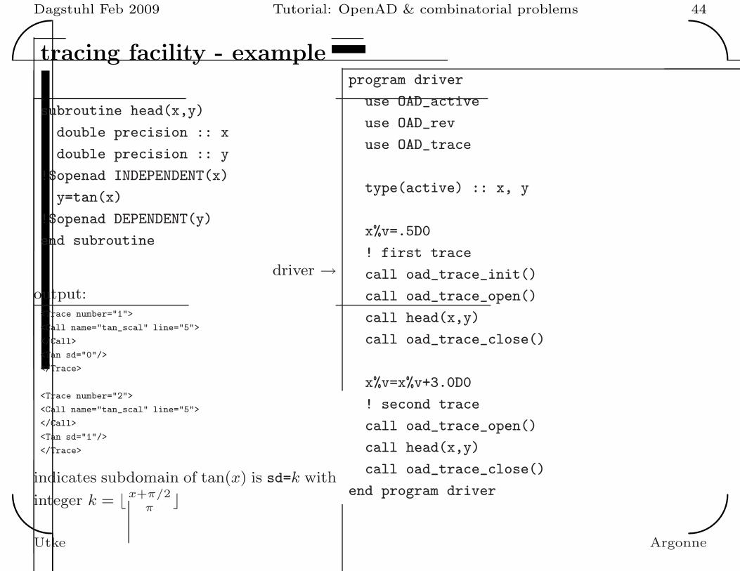
tracing facility - example


double precision :: x

double precision :: y


y=tan(x)


end subroutine

driver →

output:<Trace number="1">

<Call name="tan_scal" line="5">

</Call>

<Tan sd="0"/>

</Trace>

<Trace number="2">


</Call>

<Tan sd="1"/>

</Trace>

indicates subdomain of tan(x) is sd=k with

integer k = ⌊x+π/2

π⌋

program driver

use OAD_active

use OAD_rev

use OAD_trace

type(active) :: x, y

x%v=.5D0

! first trace

call oad_trace_init()

call oad_trace_open()

call head(x,y)

call oad_trace_close()

x%v=x%v+3.0D0

! second trace

call oad_trace_open()

call head(x,y)

call oad_trace_close()

end program driver

Utke Argonne


&

$

%

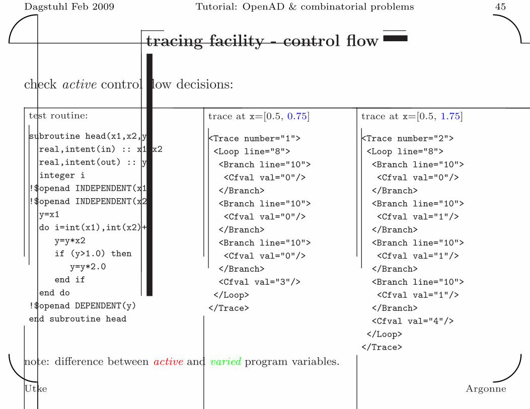
tracing facility - control flow

check active control flow decisions:

test routine:

subroutine head(x1,x2,y)

real,intent(in) :: x1,x2

real,intent(out) :: y

integer i

!$openad INDEPENDENT(x1)

!$openad INDEPENDENT(x2)

y=x1

do i=int(x1),int(x2)+2

y=y*x2

if (y>1.0) then

y=y*2.0

end if

end do


end subroutine head

trace at x=[0.5, 0.75]

<Trace number="1">

<Loop line="8">

<Branch line="10">

<Cfval val="0"/>

</Branch>

<Branch line="10">

<Cfval val="0"/>

</Branch>

<Branch line="10">

<Cfval val="0"/>

</Branch>

<Cfval val="3"/>

</Loop>

</Trace>

trace at x=[0.5, 1.75]

<Trace number="2">

<Loop line="8">

<Branch line="10">

<Cfval val="0"/>

</Branch>

<Branch line="10">

<Cfval val="1"/>

</Branch>

<Branch line="10">

<Cfval val="1"/>

</Branch>

<Branch line="10">

<Cfval val="1"/>

</Branch>

<Cfval val="4"/>

</Loop>

</Trace>

note: difference between active and varied program variables.

Utke Argonne


&

$

%

tracing facility - data

associating events with program data:

test routine:


real :: x(2),y


y=0.0

do i=1,2

y=y+sin(x(i))+tan(x(i))

end do


end subroutine

trace at x=[0.5, 0.75]

<Trace number="1">


<Arg name="X">

<Index val="1"/>

</Arg>

</Call>

<Tan sd="0"/>


<Arg name="X">

<Index val="2"/>

</Arg>

</Call>

<Tan sd="0"/>

</Trace>

trace at x=[0.5, 3.75]

<Trace number="2">


<Arg name="X">

<Index val="1"/>

</Arg>

</Call>

<Tan sd="0"/>


<Arg name="X">

<Index val="2"/>

</Arg>

</Call>

<Tan sd="1"/>

</Trace>

note: no arguments recorded w/o address computation...

Utke Argonne


&

$

%

tracing facility - call stack

need call stack context (shown by nesting):

test routine:

subroutine foo(t)

real :: t

call bar(t)

end subroutine

subroutine bar(t)

real :: t

t=tan(t)

end subroutine


real :: x

real :: y


call foo(x)

call bar(x)

y=x


end subroutine

trace at x=0.5

<Trace number="1">

<Call name="foo" line="13">

<Call name="bar" line="3">

<Call name="tan_scal" line="7"></Call>

<Tan sd="0"/>

</Call>

</Call>



<Tan sd="0"/>

</Call>

</Trace>

trace at x=1.0

<Trace number="2">

<Call name="foo" line="13">



<Tan sd="0"/>

</Call>

</Call>



<Tan sd="1"/>

</Call>

</Trace>

note: tracing difference only for the direct call from head, not from foo

Utke Argonne


&

$

%

model coding standard & AD tool capabilities I

obvious (by now) recommendations regarding smoothness:

• avoid introducing numerical special cases

• pathological cases at domain boundaries, initial conditions

• filter out computations outside of the actual domain (e.g.√

0)

• consider explicit logic to smooth (e.g. C1 ?) kinks and discontinuities

alternative (unimplemented) approaches:

• slopes (interval based)

• Laurent series (w different rules regarding ±INF and NaN

more details later

Utke Argonne


&

$

%

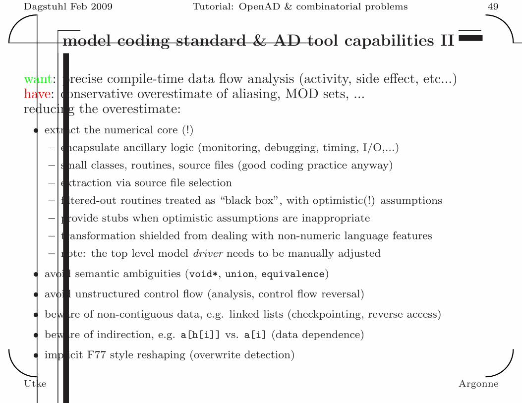
model coding standard & AD tool capabilities II

want: precise compile-time data flow analysis (activity, side effect, etc...)have: conservative overestimate of aliasing, MOD sets, ...reducing the overestimate:

• extract the numerical core (!)

– encapsulate ancillary logic (monitoring, debugging, timing, I/O,...)

– small classes, routines, source files (good coding practice anyway)

– extraction via source file selection

– filtered-out routines treated as “black box”, with optimistic(!) assumptions

– provide stubs when optimistic assumptions are inappropriate

– transformation shielded from dealing with non-numeric language features

– note: the top level model driver needs to be manually adjusted

• avoid semantic ambiguities (void*, union, equivalence)

• avoid unstructured control flow (analysis, control flow reversal)

• beware of non-contiguous data, e.g. linked lists (checkpointing, reverse access)

• beware of indirection, e.g. a[h[i]] vs. a[i] (data dependence)

• implicit F77 style reshaping (overwrite detection)

Utke Argonne


&

$

%

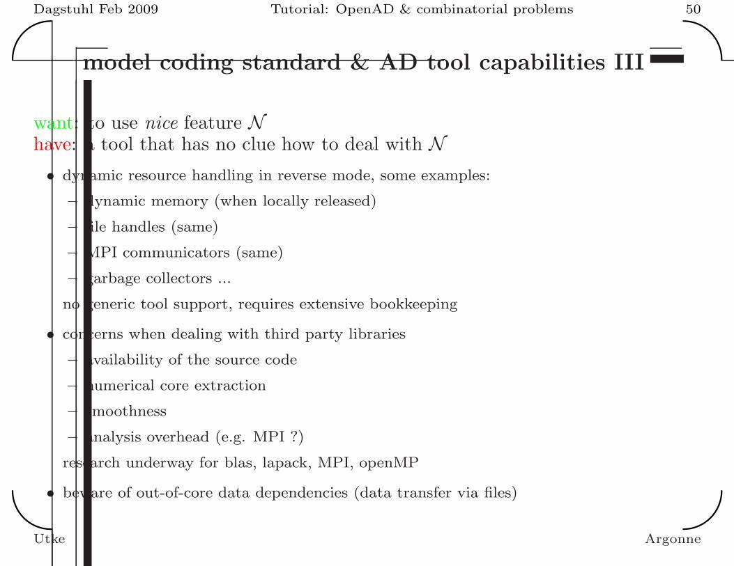
model coding standard & AD tool capabilities III

want: to use nice feature Nhave: a tool that has no clue how to deal with N• dynamic resource handling in reverse mode, some examples:

– dynamic memory (when locally released)

– file handles (same)

– MPI communicators (same)

– garbage collectors ...

no generic tool support, requires extensive bookkeeping

• concerns when dealing with third party libraries

– availability of the source code

– numerical core extraction

– smoothness

– analysis overhead (e.g. MPI ?)

research underway for blas, lapack, MPI, openMP

• beware of out-of-core data dependencies (data transfer via files)

Utke Argonne


&

$

%

further info

• http://www.mcs.anl.gov/openad

– instructions to download & build

– documentation

– revision history

– bibliography

– wiki

– bug tracker

• A. Griewank, A. Walther Evaluating Derivatives, 2nd Ed., SIAM, 2008.

• community website http://www.autodiff.org

Utke Argonne

tutorial: automatic diﬀerentiation with openad ... · dagstuhl feb 2009 tutorial: ... tutorial:...

Documents