TURBULENT SHEAR L A m R HIXING UITH FAST CHEMICAL REACTIONS

Paul E. D I M O T A K I S

Graduate Aeronautical Laboratories

California Ins t i tu te of Technology

Pasadena, California 91 125

ABSTRACT

A model is proposed for calculating molecular mixing and chemical reactions in fu l ly developed turbulent shear layers, in the l i m i t of in f in i t e ly f a s t chemical kinetics md negligible heat release. The model is based on the assumption that the topology of the interface between the two entrained reactants in the layer, as well as the s t r a i n f i e l d associated w i t h it, can be described by the s imi lar i ty laws of the Kolmogorov cascade. The calculation estimates the integrated volume fraction across the layer occupied by the chemical product, as a function of the stoichiometric mixture r a t i o of the reactants carried by the f ree streams, the velocity r a t i o of the shear layer, the local Reynolds number, and the Schmidt number of the flow. The resu l t s are in good agreement w i t h measurements of the volume fraction occupied by the molecularly mixed f lu id in a turbulent shear layer and the amount of chemical product, in both gas phase and liquid phase chemically reacting shear layers.

understanding chemically reacting, turbulent f ree shear flows is important not only

for the obvious technical reasons associated w i t h the engineering of a variety of reacting

and combusting devices but also for reasons of fundamental importance to f lu id mechanics

and our perception of turbulence.

From a theloretical point of view, chemically reacting flows provide important t e s t s

of turbulence theories by adding t o the dimensionality of the questions that can be asked

of turbulence mlodels. To compute chemical reactions in turbulent flow, the physics of

reactant species turbulent transport and mixing need t o be described correctly down t o the

diffusion scale level. This is a much more str ingent specification than needs be imposed

on momentum transport turbulence models.

From an exlperirnental point of view, a f a s t chemical reaction provides a probe w i t h an

effective spa t i a l and temporal resolution and sens i t iv i ty that is usually unattainable by

conventional d i rec t flow f i e l d measurement techniques in high Reynolds number turbulent

flows. Chemically reacting turbulent flow experiments are therefore to be regarded as a

complementary means of interrogation; a valuable adjunct to the more conventional probing

of the behavior of turbulent flow.

A broad class of current efforts to understand chemically reacting turbulent flows is

based on classical turbulence formulations founded on the Reynolds-averaged Navier-Stokes

equations. In such formulations, species transport is conventionally modeled as

proportional to the gradient of the corresponding mean species concentration, with an

effective diffusivity that is prescribed to be some function of the flow. See Tennekes &

Lumley (1972) for an introduction. Estimates of mixing at the molecular scale must be

modeled separately, in these formulations, in a manner that unfortunately cannot be

addressed without additional assumptions, that are essentially ad hoc. See Sreenivasan,

Tavoularis & Corrsin (19811, the introduction in Broadwell & Breidenthal (1982) and the

discussion in Broadwell & Dimotakis (1986) for a discussion of these issues.

A different approach is taken bjr modeling efforts based on attempts to write

transport equations for the probability density functions (E) of the conserved scalars, or joint Z s for scalars, and/or the (vector) velocity field and pressure. See Pope

(1 985 and related work by Kollmann & Janicka ( 1 982 and Kollmann ( 1 984 1, for example.

These efforts, which are in principle capable of addressing the issues of transport and

mixing in a unified manner, must nevertheless resort to essentially equally ad hoc

assumptions to close the problem. In other words, while having the correct fluctuation

statistics through the relevant E s , and conditional statistics through one-time joint

PDFs, would undoubtedly permit the molecular mixing and resulting chemical product - formation to be computed correctly, it would appear that those -s are no easier to

obtain than the ab initio solution of the original problem.

Finally, a model was recently proposed by Broadwell & Breidenthal (1982) which is not

based on gradient transport concepts. This model will be discussed below in the context

of recent data on chemically reacting shear layers in both gas phase and liquid phase

shear layers.

1 .1 Recent experimental results

The aspirating probe (Brown & Rebollo 1972) measurements of Brown & Roshko (19741,

and the measurements of Konrad (1976) of the probability density function of the high

speed fluid fraction in a non-reacting, gas phase shear layer suggested that the mixed

fluid composition does not vary appreciably across the width of the layer, even as the

mean high speed fluid fraction varies smoothly from unity on the high speed side, to zero - on the low speed side. Additionally, as Konrad recognized, the most likely values of the

mixed fluid high speed fluid fraction seem to be clustered around a value dictated by the

shear layer entrainment ratio. In the light of these results, the smooth variation of the

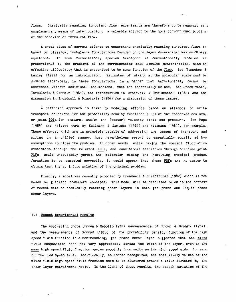
mean is then t o be understood a s the v a r i a t i o n of t h e l o c a l p r o b a b i l i t y of f i n d i n g :

a . pure high speed f l u i d ,

b. mixed f l u i d ,

and,

c . pure low speed f l u i d ,

a s we t r a v e r s e t h e width of the l a y e r .

FIGURE I . Temperature vs. time time t r a c e s f o r 4 = 1 (ATflm 93 K). High speled (U1 = 22 m/s) f l u i d (1% F2 + 99% N2) on t o p t r a c e . Low speed ( U 2 = 8.8m/s) f l u i d (1% H2 + 99% N2) on bottom. Probe p o s i t i o n s a t y/x = 0.076, 0.057, 0.036, 0.015, -0.008, -0.028, -0.049, -0.070 . P a r t i a l record of 51 .2 m s time span (ATmax = 81 K ) . From Mungal & Dimotakis (1984, f i g u r e 4b) .

The near unifcirmity i n t h e mixed f l u i d composit ion, apparent i n Konrad's pass ive

s c a l a r non-reacting; shea r l a y e r experiments, can be seen t o have an important coun te rpa r t

i n t h e gas-phase, cl?emically r e a c t i n g shear l a y e r experiments (e.g. Mungal & Dimotakis

198Q). Measuring 'the temperature f i e l d i n t h e r e a c t i o n zone of a mixing l a y e r b r ing ing

toge the r H2 and F2 r e a c t a n t s c a r r i e d i n a N2 d i l u e n t , i t is found t h a t wi th in t h e

d i s c e r n i b l e r eg ions t h a t can be a s s o c i a t e d wi th t h e i n t e r i o r of t h e l a r g e s c a l e s t r u c t u r e s

t h e temperature was nea r ly uniform. See f i g u r e 1 . The r e s u l t i n g mean temperature

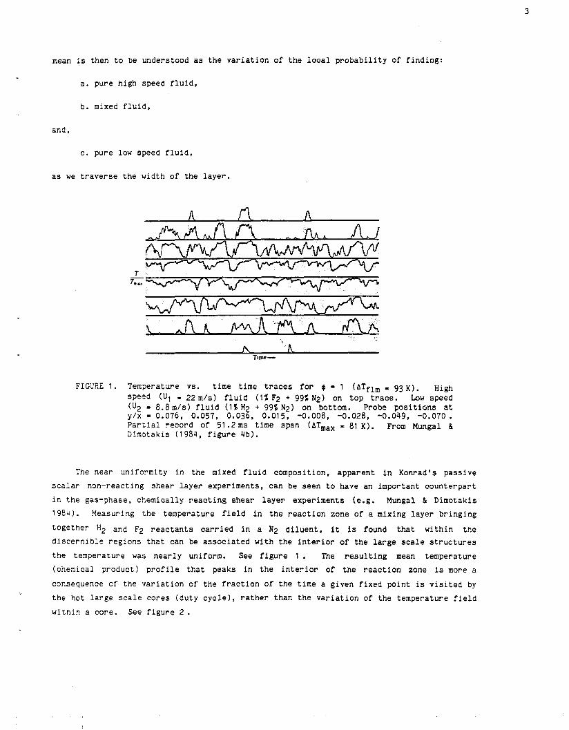
(chemical product) p r o f i l e t h a t peaks i n t h e i n t e r i o r of t h e r e a c t i o n zone is more a

consequence of the v a r i a t i o n of the f r a c t i o n of t h e t ime a given f ixed po in t is v i s i t e d by

t h e hot l a r g e s c a l e co res (du ty c y c l e ) , r a t h e r than the v a r i a t i o n of the temperature f i e l d

wi th in a core . See f i g u r e 2 .

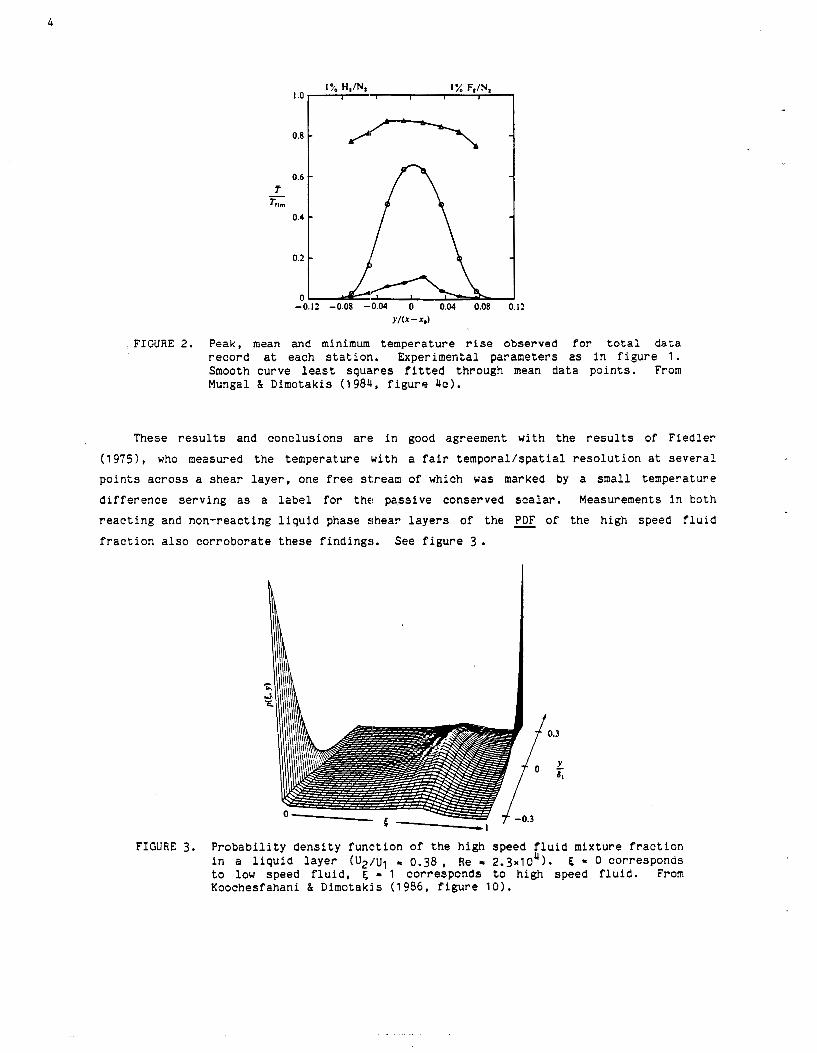
FIGURE 2. Peak, mean and minimum temperature rise observed for total data record at each station. Experimental parameters as in figure 1. Smooth curve least squares fitted through mean data points. From Mungal & Dimotakis ( 1 9841, figure 4c) .

These results and conclusions are in good agreement with the results of Fiedler

(19751, who measured the temperature with a fair temporal/spatial resolution at several

points across a shear layer, one free st:ream of which was marked by a small temperature

difference serving as a label for the! passive conserved scalar. Measurements in both

reacting and non-reacting liquid phase shear layers of the PDF of the high speed fluid

fraction also corroborate these findings. See figure 3.

FIGURE 3. Probability density function of the high speed fluid mixture fraction in a liquid layer ( U 2 / u 1 = 0.38 , Re I 2.3~104). 6 = 0 corresponds to low speed fluid, 6 = 1 corresponds to high speed fluid. From Koochesfahani & Dimotakis (1986, figure 10).

An important conclusion can be drawn from these data, which is also consistent with

the results of the flow visualization studies and the earlier pilot, liquid phase,

chemically reacting experiments in Dimotakis & Brown (19761, as well as the study of

liquid phase reacting layers by Breidenthal ( 1 981 1, namely that the large scale motion - within the cores of the shear layer vortical structures is capable of transporting a small

fluid element from one edge of the layer to the other, before any significant change in

its internal composition can occur. During this transport phase, initially unmixed fluid

within the fluid element will mix to contribute to the amount of molecularly mixed fluid,

but will do so to produce a range of compositions clustered around the value corresponding

to the relative amounts of unmixed fluid originally within the small fluid element. This

is the reason why the mixed fluid composition cannot exhibit a substantial systematic

variation across the layer and, in particular, need not be centered about the value of the

local mean. This observation represents an important simplification to the problem, as it

suggests that it may be justified to treat the composition field in a uniform manner

across the shear layer width.

In the gas phase, hydrogen-fluorine experiments of Mungal & Dimotakis (19841, the

stoichiometric mixture ratio 4, defined by

was varied, where C02 and c01 are the low and high speed free stream reactant

concentrations respectively, and the subscript 'fs'f in the denominator denotes the

corresponding chemical reaction stoichiometric ratio (unity for the H2 +E2 reaction). The

quantity 4 can be viewed as representing the mass of high speed fluid required (to be

mixed and react) to exactly consume a unit mass of low speed fluid. For uniform density,

chemically reacting shear layers (low heat release), $I can also be interpreted in terms of

the requisite volumes of the free stream fluids for complete reaction.

For a given value of $, the total amount of chemical product in the mixing layer can

be expressed in terms of the integral product thickness

where the subscript 1 in 6pl denotes that c01, the high speed stream reactant

concentration, was used to normalize the mean chemical product concentration profile

cp(y ,@). Using the mean temperature rise bT(y ,@) as the measure of product concentration,

and normalizing the transverse coordinate y by the total width of the layer 6, we can also

write

If we keep c01 fixed and vary 4 by, say, increasing c02, a l s o keeping the heat c apac i t i e s

fo r the f r e e stream f l u i d s matched, we f i n d t ha t the dependence of the ad iaba t ic flame

temperature r i s e on 4 is given by

where A T f l m ( l ) is the ad iaba t ic flame temperature r i s e corresponding t o a s toichiometr ic

reac tan t concentration r a t i o . Note t h a t , f o r a f ixed high speed stream reac tan t

concentrat ion c01, the normalizing temperature i n equation 1.3 is given by

ATflm(-) = 2 ATflm(l 1 . The experimental values f o r the product thickness 6p1/6 , i n such

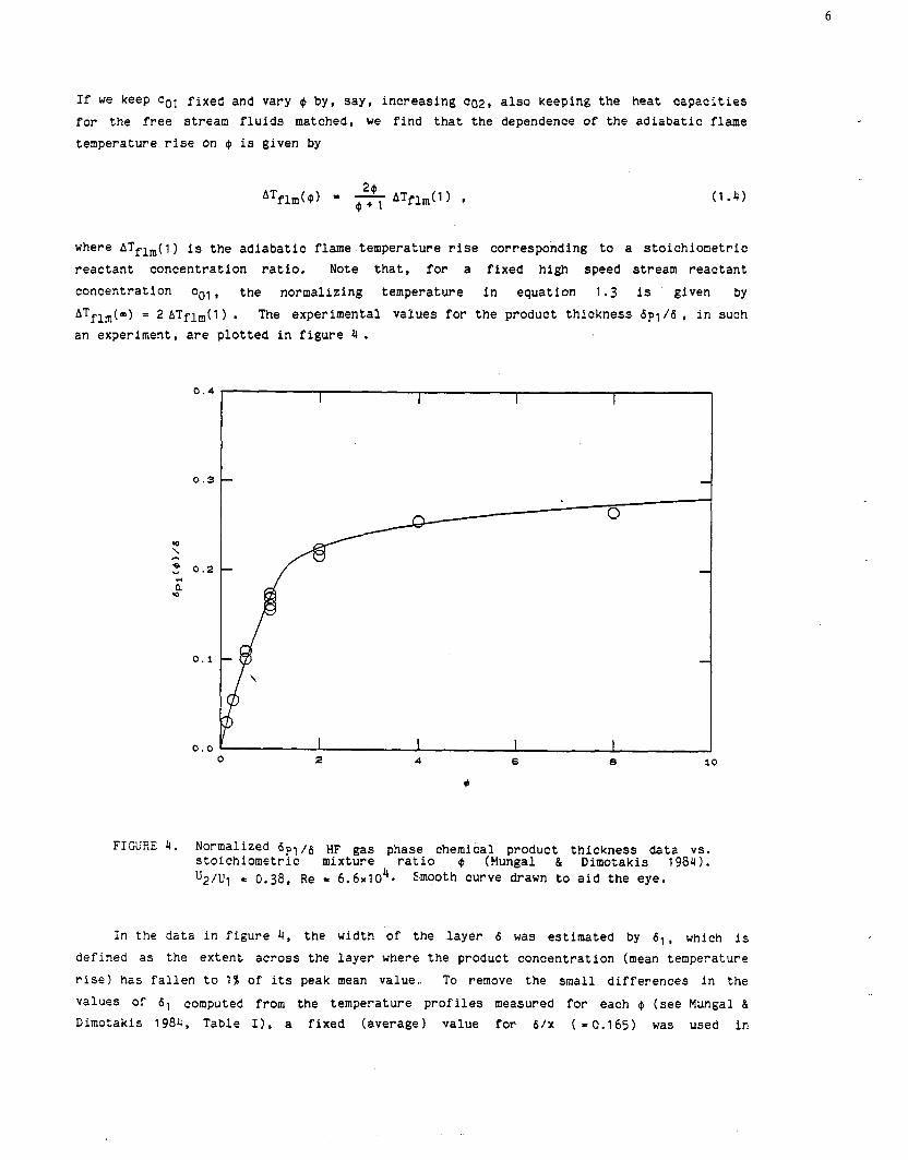
an experiment, a r e p lo t ted i n f i gu re 4 .

FIGURE 4 . Normalized 6 p 1 / 6 HF gas phascq chemical product thickness data vs. s to ich iomet r lc mlxture r a t l o 4 (Mungal & Dimotakis 1984 1. U 2 / u l 0.38, Re - 6.6x1040 Smooth curve drawn t o a id the eye.

In the data i n f igure 4, the w i d t h of the layer 6 was estimated by 6 1 , which is

defined a s the extent across the layer where the product concentration (mean temperature

r i s e ) has f a l l e n t o 1 % of its peak mean value. To remove the small differences in the

values of 61 computed from the temperature p ro f i l e s measured fo r each 6 ( see Mungal &

Dimotakis 1984, Table I ) , a f ixed (average) value fo r 6 / x ( ~0.165) was used i n

norma l i z ing t h e d a t a i n f i g u r e 4 . We n o t e t h a t t h e 1 % wid th 6 i , i n both t h e gas phase

r e a c t i n g l a y e r d a t a and t h e l i q u i d phase measurements of Koochesfahani & Dimotakis (19861,

was found t o be very c l o s e t o t h e v i s u a l shea r l a y e r width dvis of Brown & Roshko (1974).

A s can be s een i n t h e d a t a i n f i g u r e 4, a s 4 i s i n c r e a s e d from s m a l l v a l u e s , t h e amount of

chemical product a t first i n c r e a s e s r a p i d l y . Beyond a c e r t a i n v a l u e , however, a f u r t h e r

i n c r e a s e i n 4 ( i n c r e a s e o f t h e low speed s t r e a m r e a c t a n t c o n c e n t r a t i o n ) does no t r e s u l t i n

a commensurate i n c r e a s e i n t h e t o t a l chemical p roduc t , a s t h e f l u i d i n t h e s h e a r l a y e r is

low speed r e a c t a n t r i c h and much o f t h e e n t r a i n e d h igh speed s t r e a m r e a c t a n t h a s a l r e a d y

been consumed. The smooth cu rve i n f i g u r e 4 was drawn t o a i d t h e eye.

A s l i g h t l y d i f f e r e n t d e f i n i t i o n o f product t h i c k n e s s , which a v o i d s t h e asymmetric

cho ice of u s i n g one s t r eam o r t h e o t h e r a s a r e f e r e n c e , is t o use t h e a d i a b a t i c f lame

t empera tu re ATf lm($) t o normal ize the t empera tu re p r o f i l e , co r r e spond ing t o each va lue of

. T h i s y i e l d s a new normal ized product t h i c k n e s s 6 p / 6 , g i v e n by

which r e p r e s e n t s t h e volume f r a c t i o n occupied by chemical product . Note t h a t t h e

i n t e g r a n d is i n t h e u n i t s of t h e normal ized mean t empera tu re r i s e p r o f i l e , a s p l o t t e d i n

f i g u r e 2 , and t h a t bp/6 = ( 6 p 1 / 6 ) / 5 4 , where

For equa l d e n s i t y f r e e s t r e a m s , n e g l i g i b l e h e a t r e l e a s e , and a g iven free s t r eam r e a c t a n t

s t o i c h i o m e t r i c mix tu re r a t i o 0, t h e q u a n t i t y r e p r e s e n t s t h e h igh speed f l u i d volume

f r a c t i o n , i n t h e mixed f l u i d , r e q u i r e d f o r complete consumption o f both r e a c t a n t s . A

volume f r a c t i o n 5 > 5$ i n t h e m o l e c u l a r l y mixed f l u i d , f o r example, co r r e sponds t o an

e x c e s s of h igh speed f l u i d , r e l a t i v e t o t h a t r e q u i r e d by the s t o i c h i o m e t r y of t h e

r e a c t i o n , and would r e s u l t i n complete consumption o f t h e low speed r e a c t a n t i n t h e

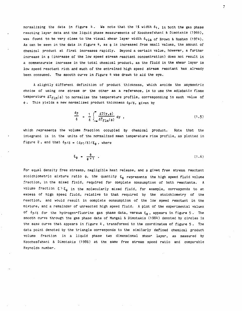
mix tu re , and a remainder of un reac t ed h igh speed f l u i d . A p l o t of t h e expe r imen ta l v a l u e s

of b p / 6 f o r t h e hydrogen-f luor ine g a s phase d a t a , Versus 56 , a p p e a r s i n f i g u r e 5 . The smooth curve through t h e g a s phase d a t a of Mungal & Dimotakis (1984) denoted by c i r c l e s is

t h e same curve t h a t appea r s i n f i g u r e 4 , t ransformed t o t h e c o o r d i n a t e s of f i g u r e 5 . The

d a t a p o i n t denoted by t h e t r i a n g l e co r r e sponds t o t h e s i m i l a r l y d e f i n e d chemical product

volume f r a c t i o n i n a l i q u i d phase two d imensional s h e a r l a y e r , a s measured by

Koochesfahani & Dimotakis (1986) a t t h e same free s t r e a m speed r a t i o and comparable

Reynolds number.

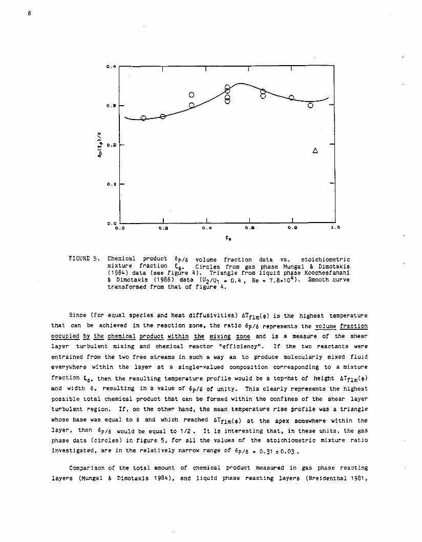
FIGURE 5. Chemical product 6 ~ 1 6 volume f r ac t i on data vs. s toichiometr ic mixture f r ac t i on 6 . C i r c l e s from gas phase Mungal & Dimotakis (1984) data ( see f i gu re 4 ) . Triangle from l i qu id phase Koochesfahani & Dimotakis (1986) data ( U 2 / u 1 0.4 , Re 7.8x104). Smooth curve transformed from t h a t of f i gu re 4.

Since ( f o r equal species and heat d i f f u s i v i t i e s ) ATflm(@) is the highest temperature t h a t can be achieved i n the reac t ion zone, t he r a t i o b p / 6 represen ts the volume f r ac t i on

occupied by the chemical product within the mixing zone and is a measure of the shear

l aye r tu rbulen t mixing and chemical rleactor wefficiencyl ' . I f the two reac tan ts were

entrained from the two f r e e streams i n such a way a s t o produce molecularly mixed f l u i d

everywhere within the layer a t a single-valued composition corresponding t o a mixture

f r ac t i on 6$, then the r e su l t i ng temperature p r o f i l e would be a top-hat of height ATflm($) and w i d t h 6 , r e su l t i ng i n a value of bp/6 of unity. This c l ea r ly represen ts the highest

poss ib le t o t a l chemical product t h a t can be formed within t he confines of the shear layer

tu rbulen t region. I f , on t he other hand, t he mean temperature r i s e p r o f i l e was a t r i ang l e

whose base was equal t o 6 and which reached ATflm($) a t the apex somewhere within the

l a y e r , then 6p /6 would be equal t o 1 / 2 . I t is i n t e r e s t i ng t h a t , i n these un i t s , the gas phase data ( c i r c l e s ) i n f i gu re 5 , f o r a l l the values of the s toichiometr ic mixture r a t i o

inves t iga ted , a r e i n the r e l a t i v e l y narrow range of b p / 6 0.31 +0.03.

Comparison of the t o t a l amount of chemical product measured i n gas phase reac t ing

l aye r s (Mungal & Dimotakis 19841, and l i qu id phase reac t ing layers (Breidenthal 1981,

Koochesfahani & Dimotakis 1986), points out another important feature of these data; at

comparable flow conditions, the amount of chemical product formed at high Reynolds numbers

is a function of the (molecular) Schmidt number Sc = v/D of the fluid, where v is the

kinematic viscosity and D is the relevant species diffusivity. In particular, roughly

twice as much product is formed in a gas phase chemically reacting shear layer (Sc = 0.8)

as in a liquid phase layer (Sc = 600).

FIGURE 6. Chemical product 6 ~ 1 6 volume fraction versus Reynolds number. Circles and squares are for gas phase data (Mungal et a1 1985) at g = 1/8. Circles are for initially laminar splitter plate boundary layers, squares for turbulent boundary layers. Triangles for liquid phase data from Koochesfahani & Dimotakis (19861, at I$ = 10.

Finally, in a further investigation in gas phase reacting shear layers, the Reynolds

number was varied over a range of almost an order of magnitude, keeping all other

conditions as constant as was feasible (Mungal et a1 1985). The resulting data for 6p/6 , for a fixed stoichiometric mixture ratio of I$ = 118, are plotted in figure 6. It can be

seen that there is a modest but unmistakeable decrease in the total amount of product in

the layer as the Reynolds number is increased. The authors estimate that, at the

operating conditions for those experiments, a factor of 2 increase in the Reynolds number (

results in approximately a 6% reduction in bp/6, the chemical product volume fraction.

Also included in the same plot, for comparison purposes, are the reacting liquid layer

data of Koochesfahani & Dimotakis (1986) at a stoichiometric mixture ratio of @ = 10. As

can be seen, the data indicate a much weaker Reynolds number dependence of the liquid

phase product volume fraction 6p/6 . We note, however, that the lower Reynolds number

liquid data point may be at a value of the Reynolds number that is too close to the shear

layer mixing transition (Konrad 1976, Bernal et a1 1979, Breidenthal 1981) and the flow

may not have attained fully turbulent behavior.

1.2 Entrainment ratio for a spatially pawing shear layer

An important conclusion drawn by Konrad (1976) was that a spatially growing shear

layer entrains fluid from each of the two free streams in an asymmetric way, even for

equal free stream densities. In particular, for equal free stream densities (p2ipl = 1 )

and a free stream speed ratio of U2/u1 = 0.38, Konrad estimated the volume flux

entrainment ratio E to be 1.3. For a free stream density ratio of p2/p1 - 7 (helium high speed fluid and nitrogen low speed fluid), and the same velocity ratio, he estimated an

entrainment ratio of E = 3.4.

This behavior can be understood in terms of the upstream/downstream asymmetry that a

given large scale vortical structure sees in a spatially growing shear layer. Simple

arguments suggest that the volume flux entrainment ratio can be estimated and is given by

where 1/x is the large structure spacing to position ratio. See Dimotakis (1986) for the

arguments leading to this result.

Konradvs data support the hypothesis that <!L/x>, the ensemble averaged value of 1/x,

is independent of the free stream density ratio p2/p1 . Fitting available data for E/x,

one finds that the relation

where r = U2/IJI is the free stream spteed ratio, is a good representation for this quantity. It can be verified that equations 1.7 produce estimates for E that are in good

agreement with Konrad's measurements. Finally, we note that to the extent that 1/x is a

fluctuating quantity, we would expect, om the basis of equation 1.7a. that the entrainment

ratio E should exhibit corresponding fluctuations. We will develop this idea in the

discussions to follow and incorporate its consequences in the proposed model calculations.

In the context of chemically reacting flows, it is important to recognize that fluid

homogenized at the entrainment ratio E produces a (high speed fluid) mixture fraction EE

given by,

For E > 1, as is always the case for matched density free streams, this corresponds to a value for EE that is greater than 1 / 2 . The resulting mixture fraction SE has a special significance in the shear layer, as Konrad recognized, and helps explain the large

differences in the composition fluctuations between his equal free stream density data and

his helium/nitrogen free stream data. See sketch and discussion on page 27 in Konrad

(1 976).

This picture suggests a zeroth order model for mixing in a two-dimensional shear

layer in which the reactants are entrained at the ratio E, as dictated by the large scale

dynamics, and eventually mixed to a (nearly) homogeneous composition in which the

distribution of values 5 of the resulting mixed fluid mixture fraction is clustered around

SE by the efficient action of the turbulence. A useful cartoon is that of a bucket filled by two faucets with unequal flow rates, as a laboratory stirring device mixes the

effluents. For all the complexity of the ensuing turbulent motion, we would expect to

find a distribution of mixed fluid compositions in the bucket clustered around the value

of the mixture fraction given by equation 1.8, where E , in our cartoon, would correspond

to the ratio of the flux from each of the two faucets. In fact, as the the faucet flow

rate is decreased relative to the mixing rate, the mixed fluid composition probability

density function is tightened around the value EE, with p(5-d~ + 6 ( ~ - SE) df i~ the limit.

The asymmetric entrainment ratio also helps explain the outcome of the chemically

reacting "flip" experiments, as they have been coined. In particular, it is known that if

the concentration of the reactants carried by the two free streams corresponds to a

stoichiometric mixt,ure ratio (O + 1 , then one obtains more or less total chemical product, depending on whether or not the lean reactant is carried by the free stream fluid that is

preferentially entrained. This can be seen in the gas phase reacting shear layer data

pairs for (O = (1/4, 4 ) and (O 9 (1/8, 81, which correspond to "flippingll the side on which

the lean reactant is carried. Compare the coresponding pairs of values for 6p/6 in the

data in figure 5. See figures 9 and 17, and related discussions in Mungal & Dimotakis

(19841, and also the liquid phase l1flip" experiments documented in Koochesfahani et a1

(1983), and in Koochesfahani & Dimotakis (1986) for additional information and

discussions.

1.3 Broadwell-Breidenthal model

In the Broadwell-Breidenthal (1982) mixing model for the two-dimensional shear layer,

the entrained fluid is described as existing in one of three states:

1. recently entrained, as yet unmixed fluid from each of the two free streams,

2. homogeneously mixed fluid at a composition SE corresponding to the entrainment

ratio E (equation 1.81,

and,

3. fluid mixed at strained laminar interfaces (flame sheets).

In this picture, the total chemical prod~~ct is computed as the sum of the contributions

corresponding to the homogeneously mixed fluid, and the contribution from the flame

sheets.

FIGURE 7. Normalized temperature rise for free stream fluids at a stoichiometric mixture fraction E,+, - ,+, / ( ,+,+I) : as a function of the high speed mixture flraction 5. Dashed triangle indicates correspondding function for a "flip" experiment and the resulting temperature rise for a mixture at the entrainment mixture fraction EE = E/(E+l).

The volume fraction in the reaction zone, corresponding to the homogeneously mixed

fluid at 5 = SE, has experienced a temperature rise (product concentration) ATH(SE,S,+,),

where, for a fixed low speed stream reactant concentration, ATflm(,+,) is given by equation

4 @H(E~,E+) is the dimensionless temperature rise, normalized by the adiabatic flame temperature rise, that results when the two fluid elements at a stoichiometric mixture

ratio t$ are homogenized to form a mixture fraction equal to the entrainment mixture

fraction SE. This is given by

corresponding to the complete consumption of the lean reactant as a function of the

resulting composition CE. See figure 7.

The heat released (amount of product) in the strained laminar interfaces (flame

sheets), for equal species and heat diffusivities, is found proportional to

where F ( S + ) is the Marble flame sheet function (Marble & Broadwell 19771, and given by

In this expression, z+ is implicitly defined by the relation

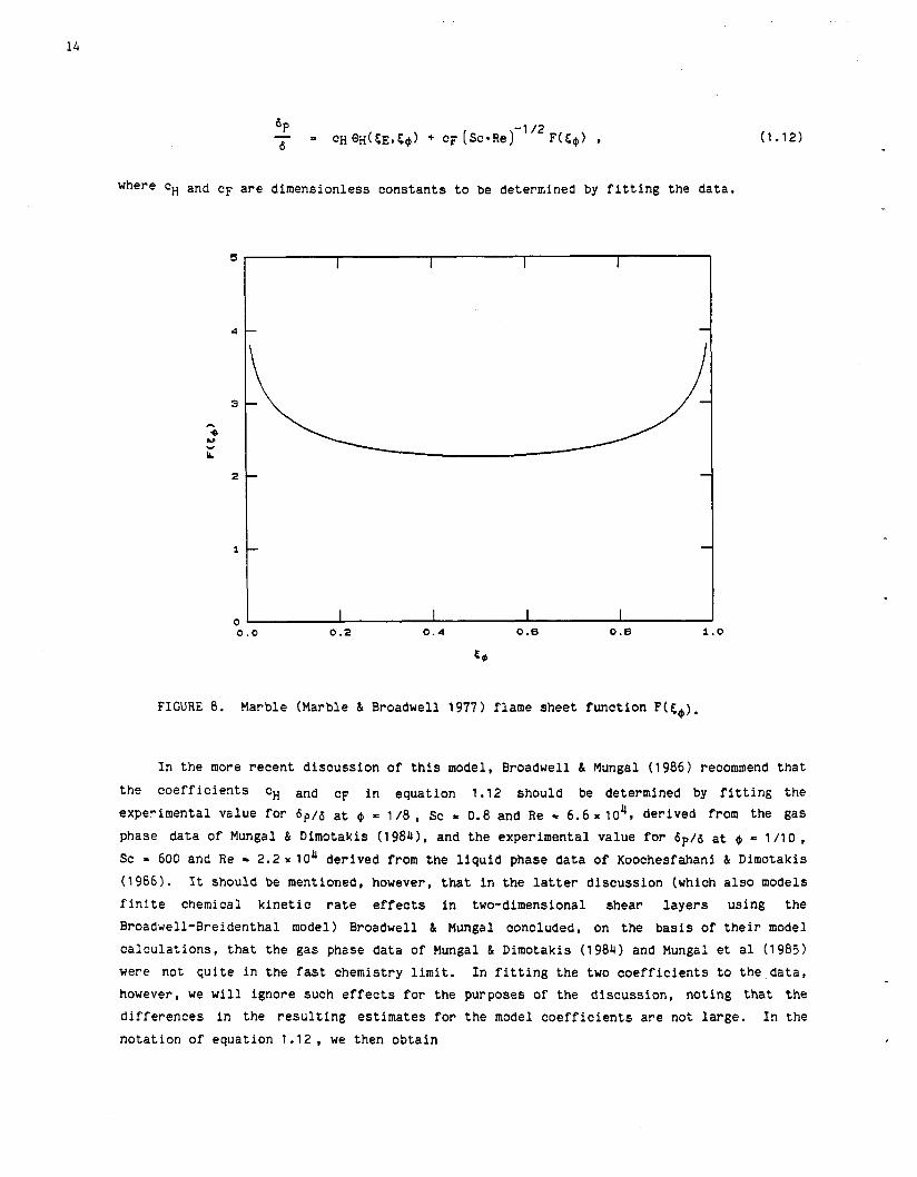
where erf(z) is the error function. The flame sheet function F(S+) is plotted in figure

8. We note here that in the original discussion (Broadwell & Breidenthal 19821, the

exponent for the Reynolds number dependence could be taken as -1/2 or -3/4, depending on

whether the appropriate flame sheet strain rate was estimated from the large scales of the

flow or the small (Kolmogorov) scales, respectively. The Reynolds number exponent is

taken here (equation 1 .lo) as - 1/2 , corresponding to the large scale strain rate,

following the recommendation in the revised discussion of this model in Broadwell & Mungal

(1986).

The contributions from the homogeneously mixed fluid and the mixed fluid on the flame

sheets should be added. Normalizing the total amount of product with ATflm(+), as in

equation 1.5, we obtain the Broadwell-Breidenthal expression for the product volume

fraction, i.e.

6~ -1 /2 - = CH OH(&,&@) + cF (SC-~e) F(5$) 6 (1.12)

where CH and CF are dimensionless constants to be determined by fitting the data.

FIGURE 8. Marble (Marble & Broadwell 1977) flame sheet function F(E$).

In the more recent discussion of this model, Broadwell & Mungal (1986) recommend that

the coefficients CH and CF in equation 1.12 should be determined by fitting the

experimental value for bp/6 at @ = 118 , sc 0.8 and Re = 6.6 lo4, derived from the gas

phase data of Mungal & Dimotakis (1984). and the experimental value for bp/6 at @ = 1/10,

Sc = 600 and Re - 2.2 x lo4 derived from the liquid phase data of Koochesfahani & Dimotakis

(1986). It should be mentioned, however, that in the latter discussion (which also models

finite chemical kinetic rate effects in two-dimensional shear layers using the

Broadwell-Breidenthal model) Broadwell & Mungal concluded, on the basis of their model

calculations, that the gas phase data of Mungal & Dimotakis (1984) and Mungal et a1 (1985)

were not quite in the fast chemistry limit. In fitting the two coefficients to the data,

however, we will ignore such effects for the purposes of the discussion, noting that the

differences in the resulting estimates for the model coefficients are not large. In the

notation of equation 1.12, we then obtain

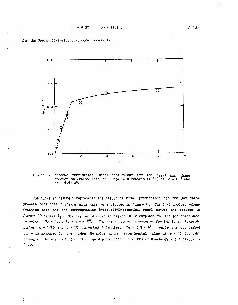
C ~ = 0 . 2 7 , c ~ " 1 1 . 5 ,

for the Broadwell-Breidenthal model constants.

FIGURE 9. Broadwell-Breidenthal model predict ions for the 6p1 /6 gas phase product thickness data of Mungal & Dimotakis (1984) at Sc = 0.8 and Re = 6.6~104.

The curve in figure 9 represents the resulting model predictions for the gas phase

product thickness bpi ($)/6 data that were plotted in figure 4 . The 6p/6 product volume

fraction data and the corresponding Broadwell-Breidenthal model curves are plotted in

figure 10 versus 5 @ . The top solid curve in figure 10 is computed for the gas phase data

(circles; Sc = 0.8 , Re = 6.6 x 10"). The dashed curve is computed for the lower Reynolds

number Q = 1 /I0 and Q * 10 (inverted triangles; Re = 2.3 x lo4), while the dot-dashed

curve is computed for the higher Reynolds number experimental value at @ = 10 (upright

triangle; Re = 7.8 x lo4) of the liquid phase data (Sc = 600) of Koochesfahani & Dimotakis

(1986) .

FIGURE 10. Broadwell-Breidenthal model predictions for b p / b vs. datfj. Solid line for gas phase data (circles; Sc = 0.8, Re =C%.6x10 , Mungal & Dimotakis 1984). Dashed line for liquid phase (Sc = 600, Koochesfahani h Dimotakis 1986) data (inverted triangles; Re r 2.3~10~). Dot-dashed line for higher Reynolds number point (upright triangle; Re = 7.8~10~).

It can be seen that several features of the reacting shear layer data can be

accounted for by this model. For a given Reynolds number, the l / f i Schmidt number dependence of the flame sheet part renders its contribution in a liquid (Sc - 600) negligible ( - 25 times smaller) as compared to that in a gas (Sc - 1 ) . Secondly, we can

see that even though the flame sheet contribution is symmetric with respect to a change

from @ to I / @ , i.e. F(&@) = F(l-c@), the homogeneous mixture contribution is not, Since

Q ~ ( ~ ~ , l - ~ g ) = OH(EE,&+) / E (compare the solid triangle function with the dashed triangle function in figure 7 ) . This allows the outcome of the experiments to be

accommodated. We note here that, for values of the stoichiometric mixture ratio + close

to the entrainment ratio E, the model predicts a relatively smaller difference for the

product volume fraction between gases and liquids, than for small (or high) values of @. Unfortunately, no relevant chemically reacting liquid phase data are available at present

to provide a direct assessment of Schmidt number effects in this regime.

'IGURE 11. Broadwell-Breidenthal model predictions for bp/6 dependence on Reynolds number. Solid curve for gas phase data (Mungal et a1 1985) at q~ = 1/8. Dashed curve for liquid phase data (Koochesfahani & Dimotakis 1986) at @ = 1 0 . Note that curves cross as a result of the larger homogeneously mixed fluid contribution for the liquid phase data at large @.

Plots of the Broadwell-Breidenthal model predictions for the product volume fraction

versus Reynolds number are depicted in figure 1 1 along with the corresponding gas phase

' data at @ = 118 of Mungal et a1 (1985) and the liquid phase data at $ = 0 of

Koochesfahani & Dimotakis (1986). The predicted curves start at a Reynolds number of

2 x l o 4 , based on the velocity difference and the local visual width of the layer, estimated

to be the minimum Reynolds number for the quasi-asymptotic behavior to have been attained,

following the shear layer mixing transition (Konrad 1976, Bernal et a1 1979, Breidenthal

1981 1. The solid line is the model prediction for the gas phase data. The dashed line

corresponds to the model prediction for the liquid phase data. Note that the predicted

curves for the gas and the liquid phase product thickness curves are computed for the

values of the stoichiometric mixture ratio corresponding to the one used in the

experiments ( @ = 1/8 and @ = 10 respectively) and will cross at some Reynolds number as a

consequence of the larger homogeneous fluid contribution for the ($I = 10) liquid data.

There would, of course, be no crossing of the model predictions at the same @, as the gas

phase product volume fraction would always be larger than the corresponding liquid phase

estimate for each value of the Reynolds number.

It can be seen that an additional important feature of the data is well represented

by the model. Namely, the Reynolds number dependence of the product thickness for the gas

phase data is predicted to be stronger than that for the liquid data. In fact, the model

prediction is that at a Schmidt number of 600 the liquid product thickness will be almost

independent of the Reynolds number. On the other hand, it would appear that the

Broadwell-Breidenthal model predicts a Reynolds number dependence for the gas phase

product thickness that may be too strong (algebraic), when compared to the dependence of

the experimental data for the product thickness versus Reynolds number of Mungal et a1

(19851, which suggest a dependence on Reynolds number that may be closer to logarithmic

(recall that those authors Suggest a 6% drop in 6p/6, per factor of two in Reynolds

number, for the range of Reynolds numbers investigated). It may be interesting to note,

as was pointed out by these authors, that the model dependence on Schmidt number and

Reynolds number is through the product ScxRe (Peclet number) considered as a single

variable. Lastly, in the limit of infinite Reynolds number, the model prediction is that

gas phase shear layers should behave like liquids, with an asymptotic value of 6~16, the

chemical product volume fraction, given by cHeH(cE,~@).

From a theoretical vantage point, the Broadwell/Breidenthal model considers the mixed

fluid as residing in strained flame sheets, as would be appropriate for interfaces

separated from each other by distances large enough such that the composition 5 (mixture

fraction) swings from 0 to 1 across them, and as homogeneously mixed fluid, as would

perhaps be appropriate at scales of the order of the (scalar) diffusion scale AD, after

the diffusion process has homogenized adjacent layers of the entrained fluids. This

partition of the mixed fluid states is an idealization, as the actual dynamics of this

process would be expected to result in a smooth transition from one regime to the other.

The authors argue that the Lagrangian time associated with that transition is short and,

therefore, intermediate states can be neglected. It can also be argued, however, that the

volume fraction associated with the molecularly mixed fluid in this intermediate state is

not small, increasing rapidly as the diffusion scaies are approached by the force of the

same arguments, and is consequently not necessarily negligible.

Another related difficulty of the Broadwell/Breidenthal model, in my opinion, is the

assignment of the volume fraction given to the homogeneously mixed fluid at 5 = SE, i.e.

the value of the coefficient CH in equation 1.12. According to the model, CH is a

constant that, in particular, is independent of both Schmidt number and Reynolds number.

It is reasonable to expect, however, that the fraction of the mixed fluid generated at the

scalar diffusion scales of the flow will be a function of the ratio A D / & , i.e. of the

scalar diffusion scale A D to the overall transverse extent of the flow 6.

We shall return to these issues in the discussion of the model proposed in this paper

and the comparison of its predictions with those of the Broadwell-Breidenthal model.

2.0 THE PROPOSED MODEL

The approach that is adopted in the model proposed here is that of viewing an

Eulerian slice of the spatially growing shear layer, at a downstream station in the

neighborhood of x, and imagining the instantaneous interface between the two

interdiffusing and chemically reacting fluids as well as the associated Strain field

imposed on that interface. It is recognized that both the Eulerian state and the local

behavior of that interface are the consequence of the Lagrangian shear layer dynamics from

all relevant points upstream of the station of interest at x. It is assumed, however,

that this upstream history acts in such a manner as to produce a self-similar state at x,

whose statistics can be described in terms of the local parameters of the flow. In

particular, it is assumed that a Kolmogorov cascade process has been the appropriately

adequate description of the upstream dynamics, leading to the local Eulerian spectrum of

scales and associated strain rate field at x.

The justification for this approach is that while the large scale dynamics are all

important in determining such things as the growth rate and entrainment ratio into the

spatially growing shear layer, the predominant fraction of the interfacial area associated with the smallest spatial scales of the flow, which can perhaps be adequately dealt with in terms of universal similarity laws. The large scales, therefore, are to be

viewed as the faucets in our cartoon, feeding,the reactants that are entrained at some

upstream station into the smaller scale turbulence at the appropriate rate. These

reactants subsequently get processed by the evolution of the cascade processes upstream to

produce the local spectrum of scales at x (see discussion in Broadwell & Dimotakis 1986).

This conceptual basis is also aided by the notion of a conserved scalar, according to

which the state of diffusion and the progress of an associated chemical reaction, in the

limit of fast (diffusion-limited) chemical kinetics, is completely determinable by the

local (Eulerian) state of the conserved scalar. See, f-r example, Bilger (1980) for a

more complete description of this notion.

An important part of the proposed procedure is the normalization that will have to be

imposed on the statistical weight (contribution) of each scale A to the total amount of

molecularly mixed fluid and associated chemical product. This is done via the expected

interfacial surface per unit volume ratio that must be assigned to each scale A . When

totalled over all scales, these statistical weights must add up to unity.

The results are first obtained conditional on a uniform value of the dissipation rate

E . An attempt to incorporate and assess the effects of the fluctuations in the local

dissipation rate f(x,t) will be made by folding the conditional results over a probability

density function for E .

In a similar vein, a refinement of the entrainment ratio idea is proposed, as noted

earlier, in which it is recognized that the large scale spacing 9./x is a random variable

and that therefore, by the force of equation 1.7a, the entrainment ratio is itself a

random variable of the flow. Accordingly, the results will be obtained conditional on a

given value of the entrainment ratio El and will subsequently be folded over the expected

distribution of values of E about its average value F.

In the calculations that follow, it is assumed that the molecular diffusivities for

all relevant species are equal to each other, but not necessarily equal to the kinematic

viscosity. Heat release effects and temperature dependence effects of the molecular

transport coefficients are also ignored. This is appropriate for the liquid phase

measurements of Koochesfahani & Dimotakis (1986), and may be adequate for the description

of the gas phase measurements of Mungal & Dimotakis (1984) and the Reynolds number study

of Mungal et a1 (1985). The issue of heat release effects on the flow was specifically

addressed elsewhere (see Hermanson et a1 1987). In computing the temperature

corresponding to the heat released in the reaction, equal heat capacities are also assumed

for the two fluids brought together within the mixing zone. While some of these

assumptions are not necessary for the proposed formulation outlined below, they allow

calculations to b.e performed in closed form permitting, in turn, the examination of the

dependence of the results on the various dimensionless parameters of the problem.

The proposed procedure assumes that the relevant statistics of the velocity field are

known (or can be estimated) and computes the behavior of the passive scalar process in

response to that velocity field. Finally, the procedure is mclosedw in that it yields the

(absolute) chemical product volume fraction 6 p / 6 in the shear layer at x , with no

adjustable parameters.

2.1 Turbulent diffusion of an entrained conserved scalar

Consider the shear layer as it entrains fluid from each of the two free streams and

is interlaced with the resulting interfaces formed between the interdiffusing free Stream

fluids into a T~vanilla-chocolate cake jelly rollw like structure. In describing the

ensuing interdiffusion process it is useful to consider the scalar concentration field of,

say, the high speed fluid mixture fraction c(&,t), where 5 = 0 represents pure low speed

fluid and f = 1 represents pure high speed fluid. A space curve intersecting the

interface of the two interdiffusing fluids everywhere normal to this interface, i.e. in

the direction of the local gradient of ~(h,t), would see at an instant in time a

concentration field E(s,t), where s is the arc length along the space curve. See figure

12. Note that, for an entrainment ratio E of high speed fluid relative to low speed

fluid which is greater than unity, we would expect that the intervals along the space

curve for which 6 - 1 , labeled "aTT in figure 12, would be longer, on average, than the

intervals labeled "b", for which 5 - 0. In fact, the ratio of the expected 5 > SE time "aT' to total time l1a + bql for adjacent layers would be given by

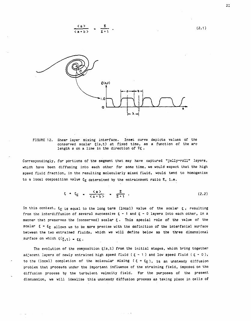
FIGURE 12. Shear layer mixing interface. Inset curve depicts values of the conserved scalar E(s,t) at fixed time, as a function of the arc length s on a line in the direction of 05.

Correspondingly, for portions of the segment that may have captured vjelly-roll" layers,

which have been diffusing into each other for some time, we would expect that the high

speed fluid fraction, in the resulting molecularly mixed fluid, would tend to homogenize

to a local composition value FE determined by the entrainment ratio E, i.e.

In this Context, SE is equal to the long term (local) value of the scalar 5 , resulting from the interdiffusion of several successive 5 - 1 and E - 0 layers into each other, in a manner that preserves the (conserved) scalar 5. This special role of the value of the

scalar 5 a 5~ allows us to be more precise with the definition of the interfacial surface

between the two entrained fluids, which we will define below as the three dimensional

surface on which F,(x,~; - I FE,

The evolution of the composition ~(s,t) from the initial stages, which bring together

adjacent layers of newly entrained high speed fluid ( 5 - 1 ) and low speed fluid ( 6 - 0 1,

to the (local) completion of the molecular mixing ( 6 + EE), is an unsteady diffusion

problem that proceeds under the important influence of the straining field, imposed on the

diffusion process by the turbulent velocity field. For the purposes of the present

discussion, we will idealize this unsteady diffusion process as taking place in cells of

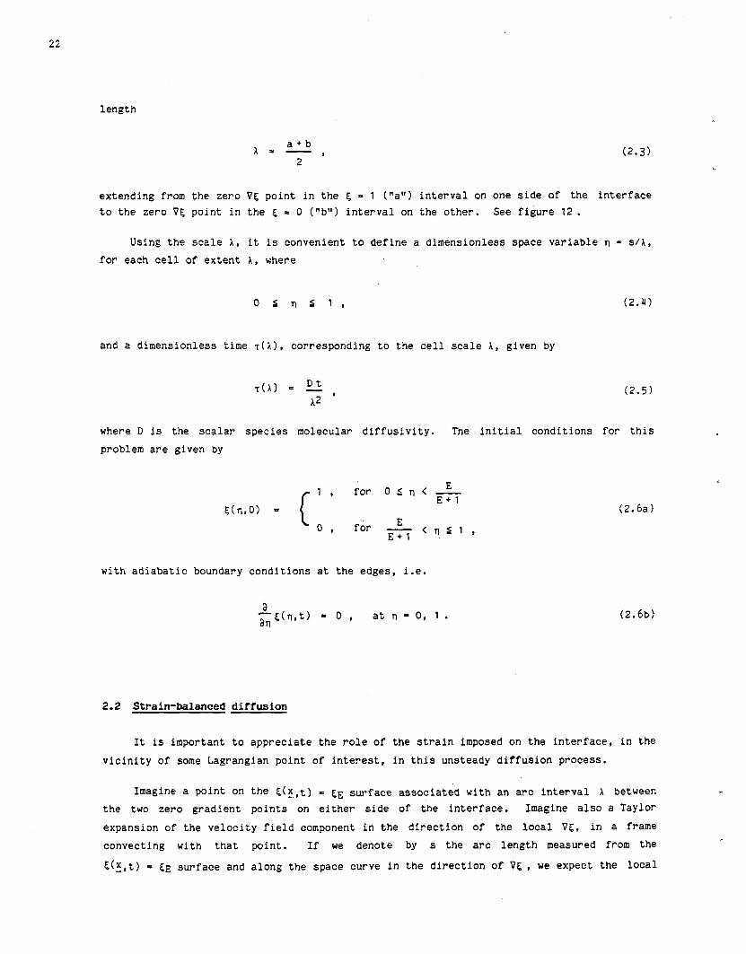
length

extending from the zero VE, point in the E, = 1 (I1a") interval on one side of the interface

to the zero Vg point in the 5 = 0 ("b") interval on the other. See figure 1 2 .

Using the scale A, it is convenient to define a dimensionless space variable n = s/A,

for each cell of extent A, where

and a dimensionless time T(X), corresponding to the cell scale A, given by

where D is the scalar species molecular diffusivity. The initial conditions for this

problem are given by

E '0, for -

E + l < n s 1 ,

with adiabatic boundary conditions at the edges, i.e.

2.2 Strain-balanced diffusion

It is important to appreciate the role of the strain imposed on the interface, in the

vicinity of some Lagrangian point of interest, in this unsteady diffusion process.

Imagine a Point on the E ( 5 , t ) = E,E surface associated with an arc interval X between

the two zero gradient points on either side of the interface. Imagine also a Taylor

expansion of the velocity field component in the direction of the local VE, in a frame

convecting with that point. If we denote by s the arc length measured from the

g(r,t) = EE surface and along the space curve in the direction of Vc , we expect the local

expression

to be an adequate approximation for this scalar product, over the transverse extent of the

diffusing layer on either side of the interface. The quantity a(A) represents the

expected value of the local strain rate, which we should be able to approximate as

We note that o(X) is not necessarily identified here with - (13, the local maximum contraction strain rate eigenvalue, where at 2 02 2 03 ape the local strain rate tensor

eigenvalues and where 01 + a2 + a3 = 0.y = 0. We do expect that identification to represent an improving approximation as the viscous scales are approached, however, in as

much as we expect the scalar interfaces to orient themselves normal to the direction of

the local maximum contraction strain rate eigenvector in the limit of small scales, and

the approximate relation of equation 2.7 to become exact in that limit. This was assumed

by Batchelor (1959) in his discussion of the scalar spectrum at high wavenumbers, and

recently corroborated by the analysis by Ashurst et a1 (1987) of the Rogers et a1 (1986)

shear flow direct turbulence simulation data.

Returning to the unsteady diffusion problem, if the initial/boundary value problem

has been proceeding in the cell of extent X for a time t(A) that is large compared to the

reciprocal of the imposed (contraction) strain rate a(A) then the solution to the

diffusion problem becomes independent of the time t(X) and a function of the strain rate

o(A) only. See figure 13. Specifically, for o(A) >> l/t(A), the appropriate

dimensionless l'timel' for the problem is given by substituting l/o(A) for t, in equation

2.5, or

This can be seen directly from the form of the diffusion equation, i.e.

which can approximately be expressed in the local Lagrangian frame as

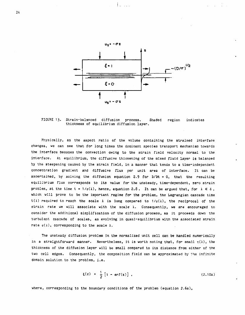
FIGURE 13. Strain-balanced diffusion process. Shaded region indicates thickness of equilibrium diffusion layer.

Physically, as the aspect ratio of the volume containing the strained interface

changes, we can see that for long times the dominant species transport mechanism towards

the interface becomes the convection owing to the strain field velocity normal to the

interface. At equilibrium, the diffusive thickening of the mixed fluid layer is balanced

by the steepening caused by the strain field, in a manner that tends to a time-independent

concentration gradient and diffusive flux per unit area of interface. It can be

ascertained, by solving the diffusion equation 2.9 for a/at + 0, that the resulting

equilibrium flux corresponds to its value for the unsteady, time-dependent, zero strain

problem, at the time t = l/o(A), hence, equation 2.8. It can be argued that, for A << 6 ,

which will prove to be the important regime for the problem, the Lagrangian cascade time

t(X) required to reach the scale X is long compared to l/o(A), the reciprocal of the

strain rate we will associate with the scale A. Consequently, we are encouraged to

consider the additional simplification of the diffusion process, as it proceeds down the

turbulent cascade of scales, as evolving in quasi-equilibrium with the associated strain

rate o(X), corresponding to the scale A.

The unsteady diffusion problem in the normalized Unit cell can be handled numerically

in a straightforward manner. Nevertheless, it is worth noting that, for small r(A), the

thickness of the diffusion layer will be small compared to its distance from either of the

two cell edges. Consequently, the composition field can be approximated by the infinite

domain solution to the problem, i.e.

where, corresponding to the boundary conditions of the problem (equation 2.6a1,

and erf(z) is the error function (equation 1.llb). ii~is result should be valid for times

T that are Short such that 5 is not appreciably different from 1 and 0 at the boundaries

n = 0, 1 respectively, in which case the approximation that the imposition of the boundary

conditions at a finite distance from the interface has not been felt as yet in the

interior of the cell is a good one.

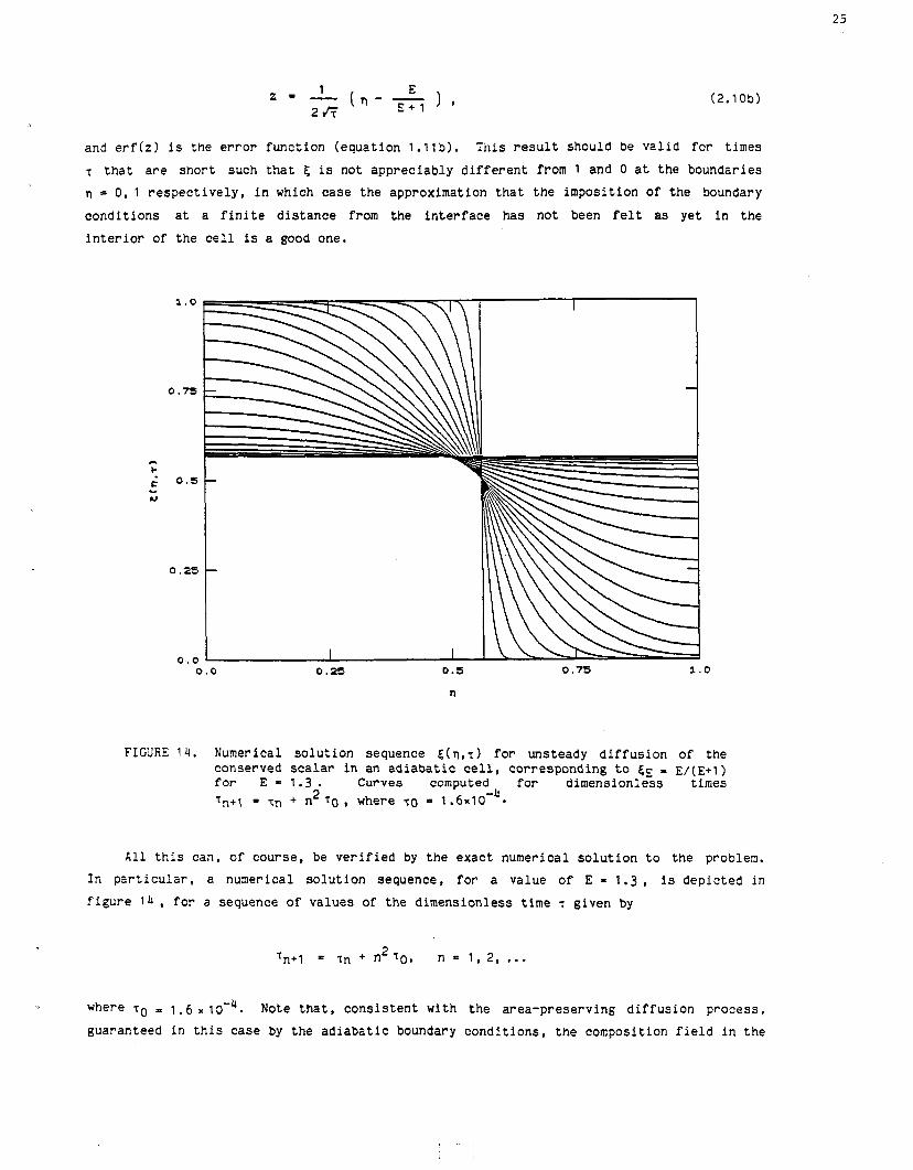
FIGURE 14. Numerical solution sequence E(~,T) for unsteady diffusion of the conserved scalar in an adiabatic cell, corresponding to EE = E/(E+I) for E = 1.3. Curves computed for dimensionless times

2 Tn+l = Tn + n TO , where r g = 1.6~10-~*

All this can, of course, be verified by the exact numerical solution to the problem.

In particular, a numerical solution sequence, for a value of E = 1.3, is depicted in

figure 1 4 , for a sequence of values of the dimensionless time T given by

where ro , 1.6 Note that, consistent with the area-preserving diffusion process,

guaranteed in this case by the adiabatic boundary conditions, the composition field in the

c e l l tends, f o r long times, t o the value .gE = E / ( E + I ) , corresponding t o the conserved

value of

( r e c a l l a l s o equation 1.8 and the r e l a t ed discussion) .

2.3 Diffusion f chemically r eac t i ng spec ies

Consider now a f a s t chemical reac t ion , w i t h neg l ig ib le heat r e l ea se , between the two

in t e rd i f fu s ing species . By f a s t here we mean tha t the thickness of the overlap region

required t o su s t a in a reac t ion r a t e , per un i t area of i n t e r f ace , t ha t can consume the

d i f fu s ive f l ux of reac tan t towards the i n t e r f ace , is small compared t o the d i f fus ion layer

thickness . I n t h i s f a s t reac t ion regime, commonly re fe r red t o a s a sdiffusion-limited"

chemical reac t ion regime, the r a t e of production is d ic ta ted by t he d i f fu s ive f lux per

un i t area towards the i n t e r f ace and not by the reac t ion k ine t i c s . More importantly,

however, a s a r e s u l t of the inter-diffusion process, wherever t he conserved s ca l a r 5 is

d i f f e r en t from 0 or 1 , the amount of chemical product formed w i l l be equal t o tha t

corresponding t o the complete l oca l consumption of the lean reac tan t i n the mixed f l u i d .

A s noted e a r l i e r , we can use temperature r i s e (heat r e l ea se ) a s a means of l abe l ing

the formation of cheemical product. In that case, the f a s t chemistry aSsumption allows us

t o compute the amount of product (temperature r i s e ) a s a funct ion of 5 , by assuming

complete consumption of the lean reac tan t . Spec i f i c a l l y , as was argued i n the case of

equation 1.9b,

C .1-5 f o r c p S 5 5 1 , 1 - Ep

where F.+ is given by equation 1.6, i.e. cp = + 1 ) , and where

is the ad iaba t ic flame temperature r i s e corresponding t o the s to ich iomet r ic mixture Pa t io

p. See f igure 15 and discussion following equation 1 .4 .

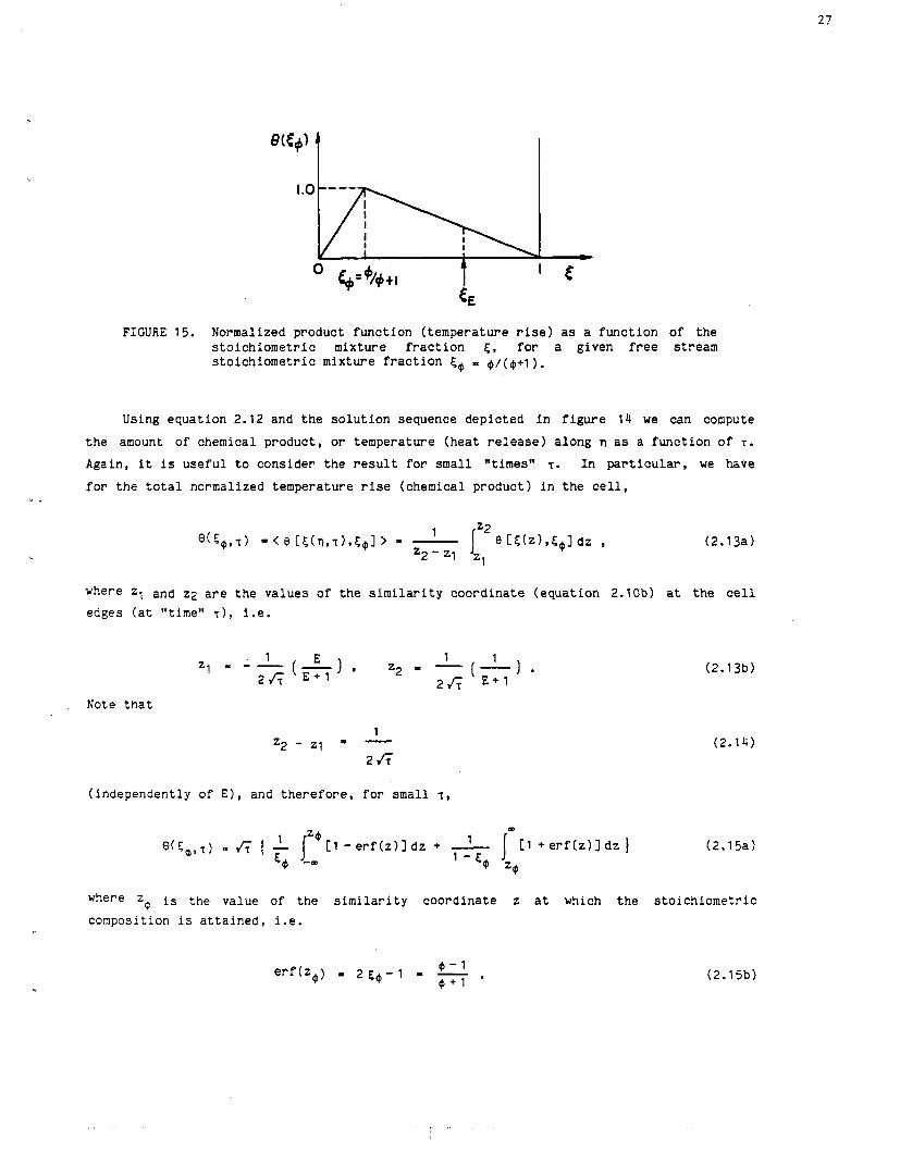
FIGURE 15. Normalized product funct ion (temperature r i s e ) a s a funct ion of the s toichiometr ic mixture f r ac t i on 5 , f o r a given f r e e stream stoichiometr ic mixture f r ac t i on E+ = $ / ( @ + I ) .

Using equation 2.12 and the so lu t ion sequence depicted i n f igure 14 we can compute

t he amount of chemical product, o r temperature (heat r e l ea se ) along n a s a function of 1.

Again, it is useful t o consider the r e s u l t fo r small "times" T. In pa r t i cu l a r , we have

f o r the t o t a l normalized temperature r i s e (chemical product) i n t he c e l l , U .

where 21 and 22 a r e the values of the s i m i l a r i t y coordinate (equation 2.10b) a t the c e l l edges ( a t "time" T I , i . e .

Note t h a t

(independently of E ) , and therefore , f o r mall 1,

where z0 is the value of the s imi l a r i t y coordinate z a t which the s toichiometr ic composition is a t t a ined , i . e .

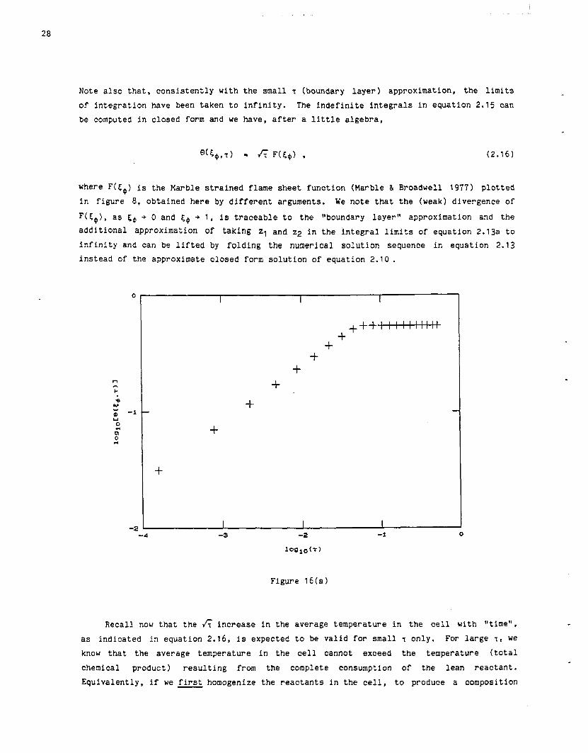
Note a l so t h a t , cons is ten t ly with the small r (boundary l aye r ) approximation, the l i m i t s

of in tegra t ion have been taken t o i n f i n i t y . The i nde f in i t e i n t eg ra l s i n equation 2.15 can

be computed i n closed form and we have, a f t e r a l i t t l e a lgebra,

where F(S$) is the Marble s t r a ined flame sheet funct ion (Marble & Broadwell 1977) p lo t ted

i n f igure 8, obtained here by d i f f e r en t arguments. We note t h a t the (weak) divergence of

F(E$), a s 5$ + 0 and E$ + 1 , is t raceable t o the *lboundary l aye rv approximation and the

addi t iona l approximation of taking 2, and z2 i n the i n t eg ra l limits of equation 2.13a t o

i n f i n i t y and can be l i f t e d by folding the numerical so lu t ion sequence i n equation 2.13

instead of the approximate closed form so lu t ion of equation 2.10.

Figure 16(a)

Recall now t h a t the fi increase i n the average temperature i n the c e l l with "time",

a s indicated in equation 2.16, i s expected t o be va l id for small T only. For l a rge T , we

know tha t the average temperature i n the c e l l cannot exceed the temperature ( t o t a l

chemical product) r e su l t i ng from the complete consumption of the lean reac tan t .

Equivalently, i f we first homogenize the r eac t an t s i n the c e l l , t o produce a composition

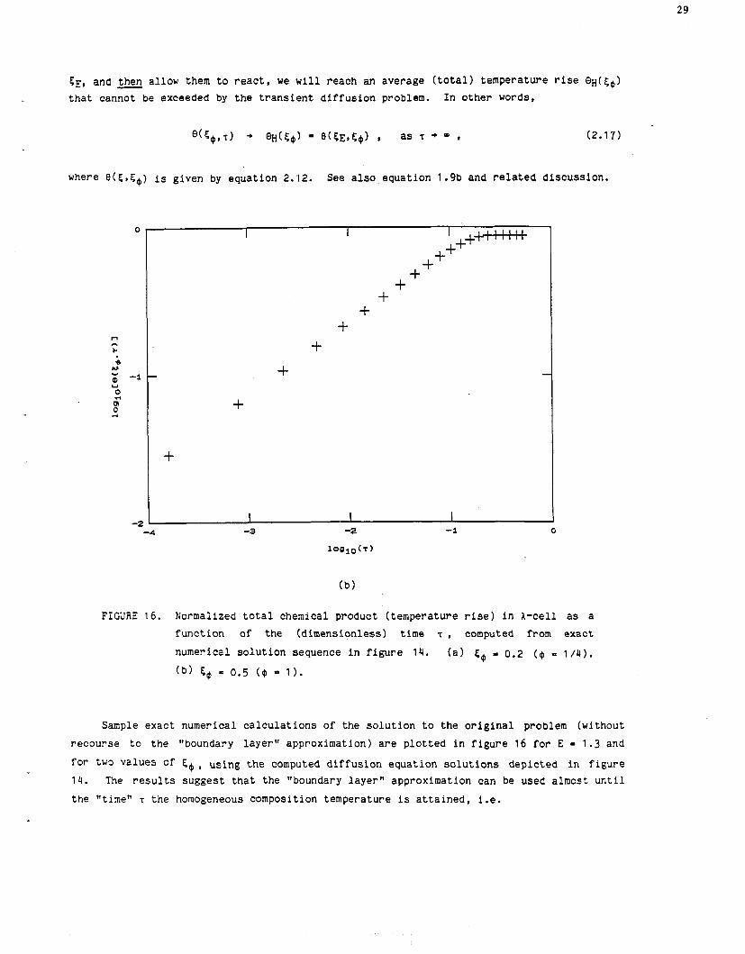
SE, and then allow them t o r e a c t , we w i l l reach an average ( t o t a l ) temperature r i s e 8 ~ ( 5 @ )

t h a t cannot be exceeded by t h e t r a n s i e n t d i f f u s i o n problem. I n o t h e r words,

where B(S,Ee) is given by equat ion 2.12. See a l s o equat ion 1.9b and r e l a t e d d i scuss ion .

FIGURE 16. Normalized t o t a l chemical product ( temperature r i s e ) i n A-cell a s a

func t ion of t h e (dimensionless) t ime 1 , computed from exact

numerical s o l u t i o n sequence i n f i g u r e 14 . ( a ) Eg - 0.2 ( 9 = 1 / 4 ) .

( b ) 5 @ = 0.5 ( @ 1 ) .

Sample exact numerical c a l c u l a t i o n s of the s o l u t i o n t o t h e o r i g i n a l problem (without

recourse t o t h e "boundary l a y e r " approximation) a r e p l o t t e d i n f i g u r e 16 f o r E = 1.3 and

f o r two values of C @ , us ing t h e computed d i f f u s i o n equat ion s o l u t i o n s dep ic ted i n f i g u r e

1 4 . The r e s u l t s suggest t h a t t h e "boundary l a y e r " approximation can be used almost u n t i l

t h e "time" T t h e homogeneous composition temperature i s a t t a i n e d , i . e .

J; F(Eg) . for T < rH @(E@,T) =

QH(s~) , for T L TH .

TH, in this approximation, is the dimensionless "timew when the homogeneous mixture total

temperature rise (completion of the reaction) is attained by the boundary layer solution.

In particular, matching the two regimes at T 5 TH, we have

See figure 17.

I I

C

r~ log T

FIGURE 17. Proposed model scaled chemical product (temperature rise) function dependence on dimensionless time T.

2.4 The scale diffusion "timew r ( A )

To proceed further, we need an estimate for u(A), the strain rate associated with the

scale A . In particular, if u(A) is the expected velocity difference across a scale A, we

have the Kolmogorov (1941) relation for the self-similar inviscid inertial range,

where E is the local dissipation rate. Consequently, for diffusion interfaces spaced by

distances A in the inertial range, the associated strain rate u(A) imposed on these

interfaces should be scaled by

We note that the highest strain rates are associated with the smallest scales.

These power laws should hold for scales A smaller than 6, where 6 is identified here

with the transverse extent of the vorticity-bearing region (6vis of Brown & Roshko 19741,

but larger than the viscous dissipation (Kolmogorov 1941) scale AK, given by

where E is the kinetic energy dissipation rate (per unit mass) in the shear layer

turbulent region. Accepting E as an integral quantity averaged over the extent 6 of the

turbulent region, and scaling with the outer flow variables, we can write

where a is a dimensionless factor. This yields a relationship between AK and the outer

variables given by

where,

is the local Reynolds number for the shear layer. We note here that the dependence of

A K / 6 on the scaled dissipation rate a is weak.

In the opposite l i m i t of small s ca l e s , corresponding t o the viscous flow X i X K

regime, the associated ve loc i ty gradients a r e imposed onto the small s ca l e s A by the

aggregate e f f ec t of the la rger s c a l e s i n the flow. In t h i s case,

and therefore ,

U ( X ) L. constant = ac , for X i X K ,

where oc is the expected contract ion s t r a i n r a t e i n the viscous regime. Consequently, we

see t h a t , i n the i n e r t i a l range, t he s t r a i n r a t e increases a s A decreases, i n accord w i t h

equation 2.20, u n t i l a maximum value is reached, corresponding t o a Scale A , . Below t h i s

s c a l e , t he associated expected s t r a i n r a t e can be taken t o be a constant.

The assumption of a scale-independent expected s t r a i n i n tne viscous range was f i r s t

proposed by Townsend (19511, who suggested ( t o quote Batchelor 19591, t h a t " the ac t ion of

the whole flow f i e l d on small-scale var ia t ions of any quant i ty ... is primari ly t o impose

a uniform pe r s i s t en t s t r a in ing motionw. This idea was used by Batchelor (1959) t o derive

t he k'l conserved temperature f l uc tua t i on spectrum i n a high Prandlt number ( P r = V / K )

f l u i d .

Gibson (1968) has argued t h a t the est imate for ac can be bracketed by the inequal i ty

where t~ = a is the Kolmogorov d i s s ipa t i on time sca l e , but notes t ha t i f f luc tua t ions i n t he l oca l d i s s ipa t i on r a t e E a r e taken i n t o account these bounds must be increased (See

a l s o Novikov 1961 and discussion i n Monin & Yaglom I 1975, end of sect ion 22.3).

Defining

and in view of the bounds in the inequa l i ty 2.25a we s h a l l accept an est imate fo r B of 3 .

Gibson's caveat , w i t h respect t o the e f f e c t of f luc tua t ions i n E , w i l l be dea l t with

below, a s the e f f e c t of f l uc tua t i ons i n the l oca l d i s s ipa t i on r a t e E w i l l be considered

e x p l i c i t l y .

Matching t o the A-2'3 behavior of o(A) i n the i n e r t i a l range (equation 2.201, we now

have f o r the expected value of a(X), over the complete range of s ca l e s ,

where Ac is a cut-off scale where the two regimes match. In other words,

A, = 83'2~K + ac = 5 . 2 ~ ~ ~ for B - 3 .

This yields for the maximum expected contraction strain rate,

and where the numerical estimate is again for 0 - 3. A sketch of u(A), versus A, is

depicted in figure 18.

I I B I

I

I I

Xk X~ log A

FIGURE 18. Proposed model contraction strain rate dependence on scale A.

Using these relations for the strain rate o ( A ) associated with the scale A, we can

now, in turn, associate the "time" r(A) to the scale A, as required by the proposed

approximate solution to the transient diffusion problem. In particular, combining

equations 2.8 for T(A) and 2.23 for a(A), we have

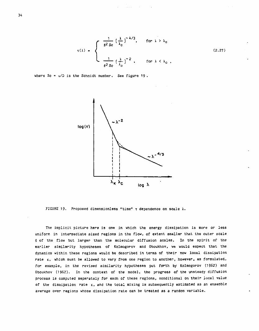
A -413 -(E) 9 f0r)i>Ac

~ ( a ) =

for A < Ac , 82 Sc

where Sc = v/D is the Schmidt number. See figure 19.

log

FIGURE 19. Proposed dimensionless "timen T dependence on scale A .

The implicit picture here is one in which the energy dissipation is more or less

uniform in intermediate sized regions in the flow, of extent smaller that the outer scale

6 of the flow but larger than the molecular diffusion scales. In the spirit of the

earlier similarity hypotheses of Kolmogorov and Oboukhov, we would expect that the

dynamics within these regions would be described in terms of their now local dissipation

rate E, which must be allowed to vary from one region to another, however, as formulated,

for example, in the revised similarity hypotheses put forth by Kolmogorov (1962) and

Oboukhov ( 1 9 6 2 ) . In the context of the model, the progress of the unsteady diffusion

process is computed separately for each of these regions, conditional on their local value

of the dissipation rate E, and the total mixing is subsequently estimated as an ensemble

average over regions whose dissipation rate can be treated as a random variable.

2.5 The reaction completion scale

The idealizations permitting the association of the unsteady diffusion "timen r with

a definite scale A, through equation 2.27, and the "time" ?H at which the homogeneous

mixture temperature BH(Q,) 'is attained (equation 2.18b). allow us to define, in turn, a

reaction completion scale AH, at which the lean reactant in the cell has been consumed and

the homogeneous temperature has been reached. Substituting in these equations, we find

that the ratio XH/Ac is determined, in turn, by the function

where F(s@) is the flame sheet function of equation 2.1 6b. In particular, we have

c[~(c4) 1 3/2 , for G(S$) > 1

We note here that the Controlling function G(s@) can be made large or small, other

things held constant, by manipulating the value of the Schmidt number. Accordingly,

corresponding to the two cases of equation 2.29 dictated by the magnitude of G(S$), we

will recognize two reacting flow regimes:

1. gas-like, for which the reaction is completed before Ac is reached, i.e. AH > A,

[ G( S+) > 1 , low SC fluid 1 ,

and

2. liquid-like, for which the reaction is completed at scales smaller than A,, i.e.

A H < A c [: G( ~ $ 1 < 1 , large Sc fluid 1 .

Combining these results with the expressions for the chemical product associated with

a particular diffusion lltimefl see equations 2.18 and 2.27, we obtain for these two

diffusion-reaction regimes,

and

where

is the dimensionless interface scale A, normalized by the strain rate cross-over scale

Ac .

2.6 The statistical weight of interface scales. Normalization.

The preceding approximations yield an estimate for the contribution to the total

chemical product in the shear layer associated with each scale A of the reactant

interface, per unit surface area associated with A . To compute the total product per

unit volume of shear layer fluid, however, we need to estimate the statistical weight W(A)

for the scale A , in the range dA, as the expected surface per unit volume of interface

associated with the scale A . Evidently, the resulting statistical weight (associated

expected total surface-to-volume ratio) over the range of scales A must be normalizable to

the unit volume, i.e.

Recall that, for every differential surface element dS Of the ~(x,t) - SE interface, the - associated scale A was defined as the arc length along 95 between the two points on either

s ide of the in te r face where 95 has decreased t o zero, o r , opera t iona l ly , t o some nominally

small f r ac t i on Y ( say , Y = 10-3) of its value a t 5 = EE. This operation is t o be

imagined a s performed fo r every element dS on the i n t e r f ace , with W ( A ) t he r e su l t i ng

probabi l i ty densi ty funct ion of A .

I t w i l l be convenient t o f i r s t consider the in te r face t ha t would be formed between

t he two entrained f l u i d s i n the absence of any s ca l a r d i f fus ion , i . e . i n the l i m i t of

Sc + m , or surface tension. It w i l l a l s o be convenient f o r the discussion below t o

f ac to r W ( A ) i n t o the surface t o volume r a t i o of a s ca l e A and the probabi l i ty p(A) of

f ind ing tha t s ca l e A i n our Eulerian s l i c e . This y ie lds the r e l a t i o n

within a normalization constant.

I f we may regard t he se l f - s imi la r i n e r t i a l range ( X c << A << 8 ) a s not possessing an

i n t r i n s i c c h a r a c t e r i s t i c s ca l e , we must accept t h a t t he (dimensionless) product W ( A ) dA

can only depend on the s ca l e X i t s e l f . Accordingly, again within a normalization

constant , we must have

as the only dimensionless, scale- invariant group t h a t can be formed between dA and A . I t -- can be seen t h a t , i n t h i s range of sca les , 5 [ l n ( ~ ) l , and therefore a l so p(A) , must be

uniform (independent of A ) , a s perhaps one might have argued a p r io r i .

I t is reasonable t o assume t h a t in te r face s ca l e s below the s t r a i n r a t e cross-over

s c a l e ic a r e pr imari ly generated within regions of extent X c o r smaller. We can imagine a b

Taylor expansion of the ve loc i ty f i e l d about the center of one such sub-Ac region and a

(non- iner t ia l ) frame of reference t h a t convects with the ve loc i ty f i e l d a t the point of

expansion, r o t a t i ng about the l oca l v o r t i c i t y a x i s a t a r a t e t ha t cancels the l oca l value

of the (nearly uniform) v o r t i c i t y i n t ha t region. I t has been a common assumption t o

regard the d i rec t ion of the pr inc ipa l s t r a i n r a t e axes as a l s o fixed in t ha t frame

(Townsend 1951, Batchelor 1959, Novikov 1961), a t l e a s t f o r a time in t e rva l of the order

of tK = (,/,)1/2. We s h a l l accept t h i s same approximation here, and a l s o assume tha t

within each of these sub-Ac regions the l oca l normal t o the s ca l a r in te r face has already

been aligned with the pr inc ipa l contract ion ax is . A s mentioned e a r l i e r , t h i s l a t t e r was

a l s o assumed by Batchelor (1959) and recent ly corroborated fo r shear flows by the ana lys i s

of Ashurst e t a1 (1987). We should note , however, t h a t the time tha t the axes need t o

s t ay fixed i n the ro t a t i ng frame is scaled by the time tDK t o d i f fu se across A K , which a t

high Schmidt numbers can be longer than tKt,

Principal Contraction Scolor /'Axis Interface I\

C J Scalor I lnterfoce

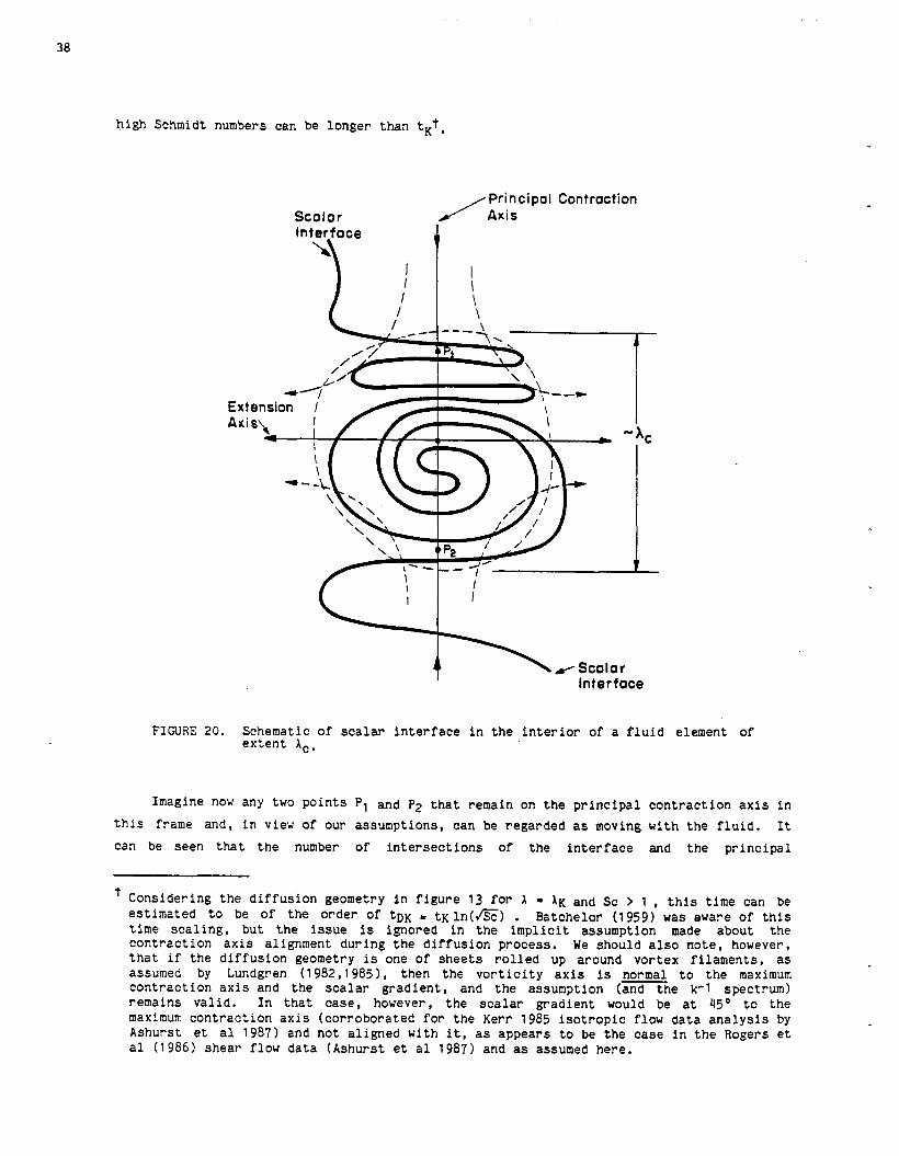
FIGURE 20. Schematic of scalar interface in the interior of a fluid element of extent Ac,

Imagine now any two Points P1 and P2 that remain on the principal contraction axis in this frame and, in view of our assumptions, can be regarded as moving with the fluid. It

can be seen that the number of intersections of the interface and the principal

' Considering the diffusion geometry in figure 13 for A = AK and Sc > 1 , this time can be estimated to be of the order of ~ D K - tr(ln(&) . Batchelor (1959) was aware of this time scaling, but the issue is ignored in the implicit assumption made about the contraction axis alignment during the diffusion process. We should also note, however, that if the diffusion geometry is one of sheets rolled up around vortex filaments, as assumed by Lundgren (1982,19851, then the vorticity axis is normal to the maximum contraction axis and the scalar gradient, and the assumption (and the k-1 spectrum) remains valid. In that case, however, the scalar gradient would be at 45' to the maximum contraction axis (corroborated for the Kerr 1985 isotropic flow data analysis by Ashurst et a1 1987) and not aligned with it, as appears to be the case in the Rogers et a1 (1 986) shear flow data (Ashurst et a1 1987) and as assumed here.

contraction axis between the points PI and Pa will be constant, as the interface geometry is strained continuously reducing the normal spacings X of the intersections of the

interface with the principal contraction axis. This conclusion is the Same regardless of

whether the interface crosses the principal contraction axis with a zig-zag sheet

topology, or as a rolled-up sheet, or a combination of these two possibilities. See

figure 20. Moreover, the subsequent reduction of the normal spacings X of these crossings

along the contraction axis will proceed in accord with equation 2.7, which we may accept

as exact for this flow regime and which we shall rewrite as

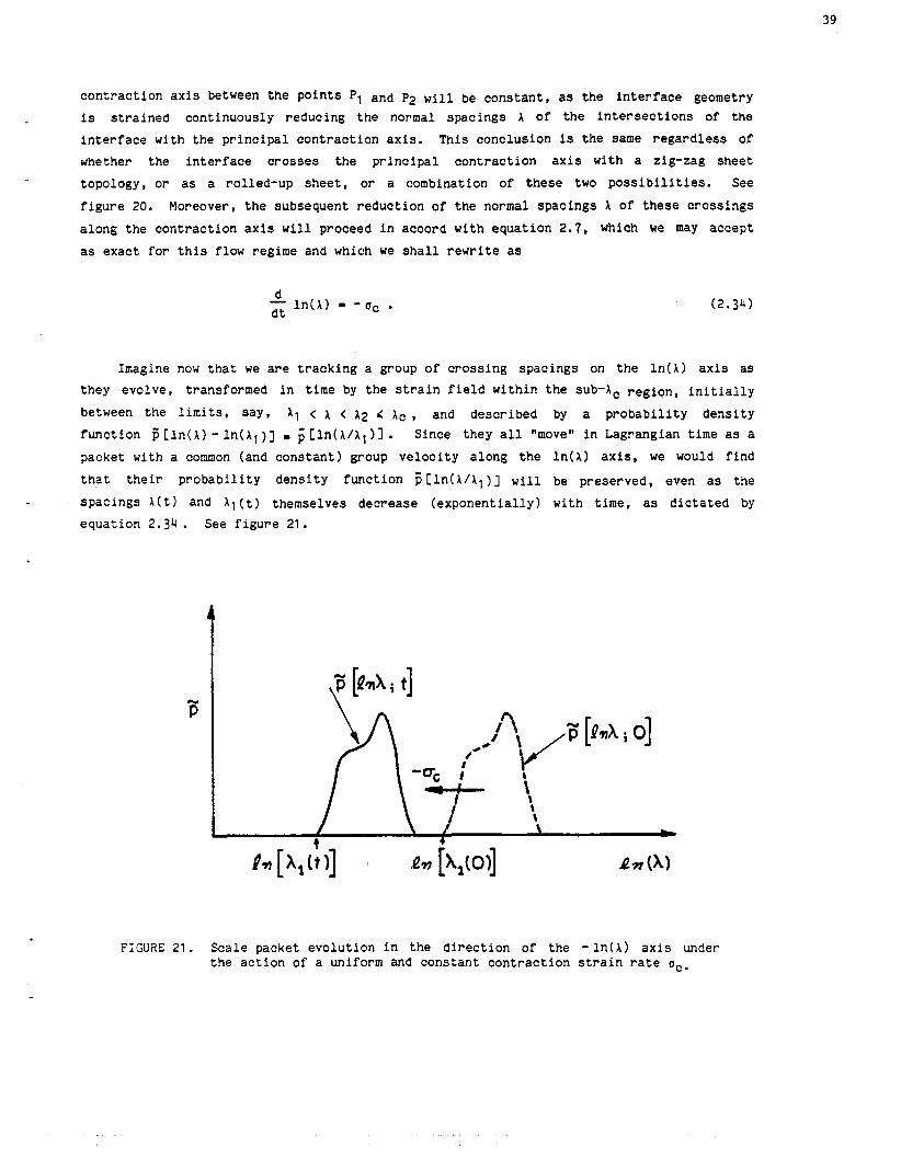
Imagine now that we are tracking a group of crossing spacings on the ln(X) axis as

they evolve, transformed in time by the strain field within the sub-Ac region, initially

between the limits, say, X1 < A < A2 L Ac , and described by a probability density function [ln(X) - ln(A,)] 5 [ln(A/X, 11. Since they all "move1' in Lagrangian time as a

packet with a common (and constant) group velocity along the ln(X) axis, we would find

that their probability density function c[ln(A/X1)] will be preserved, even as the

spacings X(t) and )Il (t) themselves decrease (exponentially) with time, as dictated by

equation 2.34. See figure 21.

FIGUAE 21. Scale packet evolution in the direction of the -ln(A) axis under the action of a uniform and constant contraction strain rate oc.

We conclude t h a t , i n t h i s sense, the s t r a in ing f i e l d i n the Sub-Ac regions does not

a l t e r the probabi l i ty densi ty funct ion 5 [ ln(A)] of the la rger s ca l e s tha t cascade t o

these regions from the i n e r t i a l range.

These arguments suggest t ha t 5 [ln(A)], and therefore a l s o p(A), must be constant not

only within the i n e r t i a l range but a l s o i n the viscous range and therefore throughout the

spectrum of the in te r face sca les . Consequently, f o r a se l f - s imi la r sur face , equation 2.33

may be accepted a s a uniformly va l id descr ip t ion of the expected sur face t o volume r a t i o

of the in te r face a s a funct ion of A , i n t he l i m i t of Sc + = .

To inves t iga te the e f f e c t of a f i n i t e Schmidt number on the associated expected

surface t o volume r a t i o of a s c a l e A , we f i r s t consider the following model problem.

Imagine t ha t we are s l i d i n g the center of a b a l l of diameter db on the Sc + m interface

and we wish t o est imate the volume swept by t h i s b a l l , per un i t volume of flow, a s its

center scans the whole surface. I t can be seen t h a t f o r port ions of the curve for which

t he l oca l s ca l e A is la rge compared w i t h the b a l l rad ius , t he volume swept w i l l be well

approximated by t he product of the b a l l diameter and the associated i n t e r f ace surface t o

volume r a t i o . Consequently, the volume swept by the ba l l a s the in te r face s ca l e

decreases , per un i t volume of f l u i d , w i l l continue t o increase in accord w i t h equation

2.33, u n t i l we reach the s c a l e A - db , below which the cont r ibu t ions per un i t in te r face

sur face area can be no la rger t ha t those a t the s ca l e A - d b . This p ic ture suggests an

est imate fo r the s t a t i s t i c a l weight of a s c a l e A , a t f i n i t e values of the Schmidt number,

given by

W ( A ) dA = 1 N(Sc,Re)

A * f o r A > XD , -.

where A D is an appropriate d i f fus ion s c a l e and N(Sc,Re) is the normalization funct ion, a s

required by equation 2.31 . In p a r t i c u l a r , i n t e g ~ a t i n g over the range of s ca l e s , we have

To proceed f u r t h e r , we need an est imate for A D / A ~ , t he r a t i o of the appropriate d i f fu s ion s ca l e t o the s t r a i n r a t e cut-off s ca l e 1,.

For high Schmidt number fluids ( Sc > 1 ) , we will base our estimate on the Batchelor

(1959) scale. In particular,

where AK is the Kolmogorov scale, 0 - 3 (recall equation 2.25 and related discussion), and CB is a dimensionless constant of order unity. To assign a numerical value to CB, we use

the Batchelor (1 959) estimates for the scalar space correlation function

which he expresses in terms of a double integral over r < r. He finds that for

distances r small compared with the diffusion scale, DES(r) - 5/6 asymptotically, whereas for distances large compared to the diffusion scale, but small compared with the

Kolmogorov scale, DSS(r) - ln(3) , where

Monin & Yaglom 111 (1975, section 22.4) express these results in terms of a differential equation for DEE('), given by

where h = h(5) is the scaled (dimensionless) DSE(r), and which can be estimated by

numerical integration of the differential equation. The rerulting solution transitions

from the linear behavior to the logarithmic behavior rather smoothly over the interval

1 5 ~ ~ 4 . Accepting the mid-point cc = 2.5 of this interval as the cross over between

the linear (diffusive) behavior and the logarithmic (convective) behavior, we obtain the

estimate CB = 6 = 1.6. Finally, expressing the diffusion scale A D in terms of the

strain rate cross-over scale A,, as required by the normalization function, we have

AD - CB - - , for S c > 1 . Sc1/2

For Sc < 1 , Batchelor, Howells & Tounsend (1959) find that XD/XK - ~c-3'~ . AS we

are not interested in Schmidt numbers that are much smaller than unity, and requiring

continuity at Sc = 1 , we will accept the estimate

C~ , for S c > l ,

AD X D s - '

Ac

, for S c < l , 0 sc3I4

with CB - 1.6 . Substituting for 6 and AD in equation 2.36, we then obtain the expression for the normalization function,

where q = 1 /2 for Sc > 1 , 314 for Sc i 1 , CB - 1.6 , 6 - 3 and a is the dimensionless

ratio of the dissipation rate c and (~~)3/6 (recall equation 2.22 and related discussion).

These considerations suggest that the problem is characterized by four length scales, namely:

. C a 1 l3 Re 1 02)3/4 Ac : large scale of the flow,

AH : reaction completion scale (equation 2.29)

Ac : strain cross-over scale, and,

AD : the species diffusion scale (equation 2.37)

All four scales have been referenced to Xc, the strain cross-over scale, related, in turn,

to the Kolmogorov scale through the constant 0 (see equation 2.26b). These scales define

the arena in which the species diffusion and chemical reaction proceeds, bounded by 6 as

the large scale limit, on the one hand, and AD as the smallest scale at which it makes

sense to attempt to track the species diffusion and chemical reaction interface.

The preceding arguments also lend credence to the conjecture that the preponderant

fraction of molecularly mixed fluid, and hence chemical product, resides on interfaces

associated with the smallest scales. This is owing to the fact that not only is the

statistical weight of the smaller scales larger (equation 2.35) but also that the chemical

product (molecularly mixed fluid) per unit surface area increases monotonically as the

scale A decreases (equation 2.30). The combination of these two effects renders the

overall description of the mixed fluid and chemical product fortuitously forgiving to the

treatment of the large scales in the flow.

2.7 The effect of dissipation rate fluctuations

The results thus far have been obtained conditional on a fixed value of the

dissipation rate E (corresponding to the particular station x). In particular, scaling

with the outer variables of the flow we wrote for the dissipation rate per unit mass

(equation 2.331,

where a is a dimensionless factor. As Landau noted soon after Kolmogorov and Oboukhov

formulated their initial similarity hypotheses, however, the local dissipation rate E (and

therefore a) cannot be treated as a constant in the turbulent region, but must be regarded

as a strongly intermittent field. This objection was addressed in the revised similarity

hypotheses of Kolmogorov (1962), Oboukhov (19621, and Gurvich & Yaglom (19671, which will

be adopted here as yielding an adequate description for the purposes of assessing the

effects of the dissipation rate fluctuations.

We can cast the revised similarity hypothesis in our notation by normalizing the - fluctuating dimensionless factor a with its mean value z, i.e. a' = a / a , such that - a' = 1 . This yields a log-normal distribution for the values of the (scaled) dissipation

rate a', averaged over a region of extent r,. In particular,

p(a'1 da' = 1 e x p j - ~ ( y - 1 ln(a') + - z 2 do' 9

6 ~ a ' 2

where Z2 = Z2(rE), is the variance of the distribution, in this model given by

The term A in this expression may depend on the large scales of the flow and u is taken as a constant.

Monin & Yaglom (1975, section 25) reviewed this hypothesis, and found that it

represents a good approximation to measurements of the local dissipation rate.

Additionally, they concluded on the basis of comparisons with data that the constant u

should be taken in the range of 0.2 5 u r 0.5. More recently, Van Atta & Antonia (1980)

considered the consequences of this proposal on the dependence of velocity derivative

moments on Reynolds number and concluded, if r, is taken all the way to the Kolmogorov

scale X K , that p should be taken as u - 0.25. Ashurst et a1 (1987) have also estimated

the value of u on the basis of direct turbulence simulation computation data (Kerr 1985,

Rogers et a1 1986) and concluded that u = 0.3. Considering all the evidence, this latter

value will be accepted as representative and as our estimate for u .

Estimates for 75, corresponding to the mean value of the dissipation r , are difficult to obtain for turbulent shear layers. There is enough information, however, in the data

of Wygnaski & Fiedler (1970) to permit an estimate of a Z 0.02. An estimate can be made

from the data of Spencer & Jones (1971 ) , which also leads to the same value. It is

difficult to assess the probable error of these estimates, not to speak of the possibility

intimated by Saffman (1968) that may not necessarily be a constant, i.e. independent of

the Reynolds number. Nevertheless, considering the nature of the experimental

difficulties, the assumptions made about isotropy, and in view of the realizable spatial

and temporal resolution relative to AK and AK / Uc, respectively, where Uc is the local

flow convection velocity, we can say that this estimate is probably low, even though

perhaps not by more than a factor of 2 to 3. Consequently, one would argue for a

plausible range of values for a of

In applying these results to the present discussion, we will take r, down to a

(fixed) viscous scale A. that is a function of the (local) Reynolds number and equal to

the strain rate field cut-off scale Ac corresponding to the mean value of the dissipation,

i.e. (see equation 2.31)

This yields an expression for the variance of a given by

Finally, an estimate can be made for the constant A with the aid of the f0110Uing argument. As the local Reynolds number is increased from very small values, the flow is

initially essentially steady with no fluctuations in the dissipation rate field. At some

minimum value of the Reynolds number, however, the flow will evolve into a fluctuating

field with a spatial scale of the order of 6 and an associated variance in the local

dissipation rate fluctuations. At that critical value of the Reynolds number we must have

z:( kCr) - 0 . This f ixes the flow-specif ic constant A, and also removes the unpleasant dependence of the variance on the particular choice of the reference scale A. , and we have

While we recognize t h a t , s t r i c t l y speaking, a f r e e shear layer does not possess a c r i t i c a l

Reynolds number, one can conclude from the l i nea r s t a b i l i t y ana lys i s f o r viscous (but

p a r a l l e l ) flow of a hyperbolic tangent p r o f i l e (Betchov & Szzewczyk 1963) t h a t an unstable

mode w i t h a s p a t i a l extent of order 6 requi res a minimum Reynolds number of the order of

15 < Re < 5 0 , which we w i l l accept a s bounds for Recr. Note t h a t Re here is based on 6 ,

t he t o t a l width of the sheared region, and not on the (smaller) hyperbolic tangent maximum

slope thickness. See a l s o discussion by Betchov (1977). I t is i n t e r e s t i n g t ha t t h i s

est imate fo r a c r i t i c a l Reynolds number is not too d i f f e r en t from the one made by Saffman

(1968), who explored the idea t ha t the s t ruc tu re of the flow i n the d i s s ipa t i on range was

e s s e n t i a l l y t h a t r e su l t i ng from the ~ a ~ l o r - ~ z r t l e r i n s t a b i l i t y of curved vortex sheets .

l o compute the probabi l i ty densi ty funct ion of the r a t i o A c / X O , we note t h a t s ince

Xc = A0 (a' 1 -1 14 , (2.448)

we must have

1 1 2 p(y) dy - e x { - ( - 2 ) } dy ,

fi where

This is cor rec t t o within a (near un i ty) normalization constant , a s we wish t o r e s t r i c t Xc

t o the range 0 4 A c 6 .

To compute the e f f e c t of the d i ss ipa t ion f luc tua t ions on the expected value of the

s ca l e s normalization funct ion N(Sc,Re) discussed i n t he preceding sec t ion , we a l s o note

t h a t i f we assume t h a t the r a t i o A c / A D IS independent of the d i s s ipa t i on r a t e E ( a

funct ion of Sc on ly) , we have

Then s ince

where

and since, in particular (at high Reynolds numbers)

1 2 xu exp 1 - F ( Y ~ - z ~ / ~ ) I

< y > = , - za = - ,

2 2 1 Yg - xa/2 JZ;; [I - -err<: (

2 fi 1 1

we have (see equations 2.38 and 2.43)

It is useful to rewrite this expression by defining a constant r through the relation

and where we note, at least on the basis of our numerical estimates for these quantities,

that r - 1 . In terms of r , we then have

Returning to the derivation of the quantity in tlhe brackets and recognizing the role it

plays in the normalization of the range of turbulent scales, however, we can argue that it

should vanish as Re + Recr and that, therefore, we must have r = 1 . This provides us

with a consistency estimate and plausible bounds for Recr (see equation 2.49a and

inequality 2.40) given by

(recall 02 - 9). This we can use to rewrite the expression for the ratio 6/A0 (equation

2.411, i.e.

Finally, for high Reynolds numbers, we may certainly ignore the ln(r) term in favor of

In (Re Recr) and we have,

where - 3 , q = 1/2 for Sc > 1 , and 314 for Sc 1 1 , CB - 1.6, - 0.3 and Recr is

bounded by the limits in equation 2.49~. It may be worth noting that the resulting

estimate for the normalization function is quite robust, as the various uncertainties in

the constants appear as arguments of logarithms.

We conclude that the effects of the dissipation fluctuations on the expected value of

the normalization function are small, being confined to the contribution to the final

result owing to a non-zero value for p .

2.8 The total product in the mixing layer

The total chemical product can now be computed as the weighted average of the

contribution of each scale, i.e.

where = A/Ac , xg = &/Ac , ~ ( x ) is given by equations 2.30 , and

for x < XD

for xD < x

(see equation 2.361, with XD = AD/Ac (see equation 2.37). We will first perform the

computations conditional on a fixed value (of the dissipation rate, and therefore Ac, and

then compute the total as the expectation value over the distribution of values of Ac.

For gas-like flow-diffusion regimes (see equation 2.30 and related discussion), we

have the relation

where G = G ( 5 + , &, Sc) is given by equation 2.28, and we need to distinguish between two cases depending on the relative values of XD and XH. The first case corresponds to

XD < XH , for which

or,

In the second case, we have XH < XD and therefore

Of these two cases, the first [ X D < xH] would typically be applicable for Sc L 1 , if 6 - 3 and we have reasonable values for the stoichiornetric mixture ratio $I and entrainment

ratio E . For liquid-like flow-diffusion regimes we have the relation

and, in principle, we need to distinguish between three cases. The first liquid-like case

corresponds to the inequalities xD < xH < 1 and the integrals

which yields

For the second liquid-like case, we have XH < XD < 1 , and

Finally, We may also have XH < 1 < xD, in which case

which yields

Of the three cases for the liquid-like regime, the first one [ xD < xH < 1 ] would

typically be applicable for Sc >> 1 . If treating the variable 0 of equation 2.25 as a constant represents an adequate

approximation, it ciin be seen that only the last ter'm in each of these expressions will be

modified by the rluctuations in the dissipation rate. With that proviso, since

~ ~ ' ~ ~ 3 = (~,/tj)~/3, the contribution of the last term is small at large Reynolds numbers.

In any event, expressing Xc/6 in terms of the corresponding distribution variable y

(equation 2.441, we find for Re >> Recr

Substituting in the results for the two typical cases (equations 2.53a and 2.54a1,

for example, we obtain for the expected value of the gas-like (G > 11, product volume fraction in the layer,

and for the typical (Sc >> 1 ) liquid-like (G < 1) product fraction

where XD is given by equation 2.37 and < x6-2/3 >E by equation 2.55.

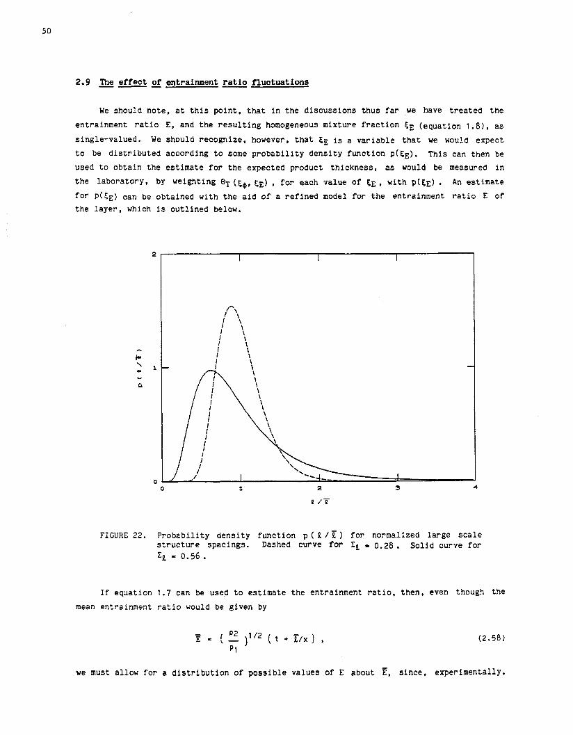
2.9 The e f f e c t of entrainment r a t i o r l u c t w t i o n s

We should note, a t t h i s point , t h a t i n t he discussions thus f a r we have t r ea t ed the

entrainment r a t i o E , and the r e su l t i ng homogeneous mixture f r ac t i on EE (€;quation 1 .8) , a s

single-valued. We should recognize, however, t h a t EE is a var iab le t h a t we would expect

t o be d i s t r i bu t ed according t o some probabi l i ty densi ty funct ion p(SE). This can then be

used t o obtain the est imate fo r t he expected product thickness , a s would be measured in

t he laboratory, by weighting 8~ (q,, cE) , fo r each value of EE, with p ( c ~ ) . An est imate

fo r p(SE) can be obtained w i t h the a i d of a ref ined model for the entrainlment r a t i o E of the l aye r , which i s out l ined below.

FIGURE 22. Probabi l i ty densi ty funct ion p ( l l / r ) f o r normalized large s c a l e s t r u c t u r e spacings. Dashed curve f o r ZL = 0.28 . s o l i d curve fo r 2, = 0.56.

I f equation 1.7 can be used t o est imate t he entrainment r a t i o , then, even though the

mean entrainment r a t i o would be given by

we must allow fo r a d i s t r i bu t i on of poss ib le values of E about E, s ince , experimentally,

FIGURE 23. Pr'obability density function for entrainment ratio mixture fraction SE = E/(E+I ). Dashed curve for = 0.28. Solid curve for z, = 0.56.

The dashed lin~e in figure 23 is the resulting probability density function p(SE),

corresponding to e~qual free stream densities, a velocity ratio of U2/u1 - 0.38 and the

Bernal value of Zk := 0.28 . Note that, in spite of the width in the J? / distribution,

the values of SE are relatively narrowly distributed about the value of SF - 0.567, corresponding to a mean entrainment ratio of F = 1.305, given by equation 2.36 for

P2/p1 = 1 and Uz/'Jl .= 0.38 . It should be noted that the experimental determination by Bernal (1981) of the

histogram of values of J? / involved the identification of the intersection of the

"braidsw of each stlnucture with the line corresponding to the trajectory of their centers.

Consequently, structures in the process of tearing or coalescence, or at any other phase

or configuration during which they could not be easily identified, were not included in

his sample population. In other words, the distribution of spacings contributing to

Bernal's experimentiel histogram and the resulting fit of the log-normal distribution width

one f i n d s t h a t t h e l a r g e s t r u c t u r e spac ing t o p o s i t i o n r a t i o Il/x is r a t h e r broadly

d i s t r i b u t e d about its mean va lue r / x . I n p a r t i c u l a r , Bernal (1981) has p re sen ted d a t a and

t h e o r e t i c a l arguments i n suppor t o f a log-normal d i s t r i b u t i o n , which we can w r i t e ,

fo l lowing t h e n o t a t i o n i n s e c t i o n 2 . 7 , a s

where

T h i s is p l o t t e d i n f i g u r e 22, where t h e dashed l i n e is computed from e q u a t i o n 2.59, u s i n g

t h e va lue recommended by Bernal of Zk = 0 . 2 8 . See Roshko (1976, f i g u r e 5 and r e l a t e d

d i s c u s s i o n ) as we l l a s Bernal (1981, f i g u r e 1 .8 ) f o r a comparison wi th expe r imen ta l d a t a .

Equat ions 1.7 and 2.58 can be combined t o y i e l d an e s t i m a t e f o r t h e expected

d i s t r i b u t i o n o f t h e va lues of t h e en t r a inmen t r a t i o E . The p i c t u r e t o be borne i n mind

is one i n which t h e en t r a inmen t r a t i o E corresponding t o a p a r t i c u l a r l a r g e s t r u c t u r e can

be t r e a t e d a s more o r l e s s f i x e d , bu t t h a t t h e va lue of E v a r i e s from s t r u c t u r e t o

s t r u c t u r e i n accordance wi th t h e range o f v a l u e s of L/x ( a s well as t h e h i s t o r y o f k/x of

t h e s t r u c t u r e s t h a t have amalgamated t o form t h e ones pas s ing through t h e s t a t i o n x ) . I n

p a r t i c u l a r , s i n c e

we have , f o r equa l f r e e s t r eam d e n s i t i e s ,

dE PE(E) dE = p , C k 9 ( ~ ) ] - E - 1

- , where E q ( E ) = - - I./X a / x

and t h e r e f o r e

Using s i m i l a r arguments, one a l s o o b t a i n s t h e d i s t r i b u t i o n p (cE) o f t h e corresponding

v a l u e s of t h e mixture f r a c t i o n EE i n te rms of pE(E) , i n p a r t i c u l a r

where, i n v e r t i n g e q u a t i o n 1 . 8 , w e have

xi was based on structures that were more or less clear of their neighbors and of interactions with them. Evidently, a full accounting of the possible large structure

spacings will contribute values of i/x, which if included in the population, would tend to

broaden its width. Moreover, the expression for the entrainment ratio as given by

equation 2.60 and as discussed elsewhere (Dimotakis 1986) refers to the entrainment flux

ratio into a single! large scale structure. The composition ratio of a given large scale

structure, however, is the one resulting from the amalgamation of Several Structures, each

of which was characterized by an entrainment ratio as dictated by its local i/x and its

fluctuations. While this consideration does not shift the mean value of E, it can be seen

that it increases the variance of E, relative to its value referenced to the fluctuations

of the local R / x . Accordingly, in estimating the distribution of values of the

entrainment ratio E, and the resulting homogeneous composition values EE, one should

accept a broader distribution of values of E , which we will approximate by accepting a

larger value of Ea . The curves depicted with the solid lines in figures 22 and 23 were computed by

doubling the Bernal value of the log-normal distribution width, i.e. Ea -0.56, as

representing a reasonable estimate for that quantity in view of the preceding discussion,

and are plotted for comparison. It can be seen, however, that even this factor of two

increase in the width ZII does not significantly alter the resulting probability density

function width for the distribution of values of EE.

Using the computed probability density function for the values of EE, the problem is

finally closed and we can now estimate the expected product thickness 6p/6 in the mixing

layer, i.e.

where <8T((E)>E is the expected value of the normalized chemical product, averaged over

the dissipation rate fluctuations, conditional on the fixed value of EE, as discussed in

the preceding section.

The dependence of the resulting estimates for bp/6 on the possible range of values of

the variance 0 1 3 is small and confined to values of the stoichiometric mixture

fraction E$ in the vicinity of SF. It will be discussed below in the context of the comparison of the theoretical values with the data.

3.0 RESULTS DISCUSSION

Using the preceding formalism, one can estimate the expected volume (or mass)

fraction of chemical product and molecularly mixed fluid generated within the

two-dimensional turbulent shear layer wedge boundaries.

We recall here that the proposed model applies to incompressible flow, i.e. in the

limit of zero Mach number. In the case of gas phase reactions, tile heat release is

assumed small and, in the case where the (small) temperature rise is used to label the

chemical product, the heat capacities of the two free stream fluids are assumed matched.

Differential diffusion effects have been ignored, i.e. all scalar species are assumed to

diffuse with the same diffusivity. Also the chemical kinetics have been assumed fast.

Finally, the Reynolds number has been assumed high enough for the shear li~yer to be in a

fully developed three-dimensional turbulent state, i.e. Re > 1 .6x104 - 2 x 1 0 ~ . In evaluating the theoretical estimates, the following values will be used for the

dimensionless parameters:

1. The expected value of the entrainment ratio F will be computed, using equation

2.58.

2. The fluctuations of E / F will be estimated using equation 2.61 with a variance

twice the Bernal value, i.e. Z i = 0.56, as discussed in section 2.9.

3. The value of the expected maximum contraction rate oc , at or below the

Kolmogorov scale, will be estimated using the expression o c t ~ = 1 1 6 with 6 - 3 (see equation 2.25 and related discussion).

4. Recr , the critical Reynolds number, will be estimated via equation 2.49~ , using the mid-point of the expected dimensionless dissipation ?; bounds (i.e. - a = 0.04). This leads to the value of Recr = 2 6 .

5. The Kolmogorov/Oboukhov coefficient p in the variance of ln(~) will be taken as

0.3 (equation 2.43).

6. The ratio XD of the diffusion scale A D to the strain rate cut-off scale )Ic will

be computed using equation 2.37, with a value of CB - 1.6, as discussed in

section 2.6.

and, finally,

7. The product volume fraction 6p /g will be computed using equation 2.63, with

<@T(s~) >, given by equations 2.56 or 2.57 (or 2.53, 2.541, as appropriate.

We note that the results are only weakly sensitive to these choices, appearing in the

final expressions, by and large, as arguments of logarithms.

3.1 Comparison G h chemically reacting flow data

The proposed model predictions for the chemical product volume fraction

6p1/6 = E4bp/6, versus the stoichiometric mixture ratio 9, for the hydrogen-fluorine gas phase data (Mungal & Dimotakis 19841, for which SC = 0.8, UZ/U1 = 0.40, p*/p1 - 1 , and Re = 6 . 6 ~ 1 0 ~ ~ are plotted in figure 24. The predicted values are in good agreement with

the gas phase chemical product volume fraction data. The essentially correct prediction

of the absolute amount of product may perhaps be regarded as fortuitous but is

nevertheless noteworthy.

FIGURE 24. Model predictions for 6p1($)/6 product thickness. Data legend as in figure 4.

A plot of the bp/6 predicted chemical product volume fraction, versus E4, appears in

figure 25. The top solid curve and data points (circles) are transformed from figure 24.

The corresponding predictions are also plotted for the liquid data (Sc = 600) of

Koochesfahani & Dimotakis (1986).

FIGURB 25. Proposed model p red ic t ions f o r b p / 6 vs. 5 d y a . Solid l i n e for gas phase data ( c i r c l e s ; Sc = 0.8, Re = 6.9.10 , Mungal L Dimotakis 1984). Dashed l i n e fo r l i q u i d phase (Sc - 600, Koochesfahani & Dimotakis 1986) da ta ( inverted t r i ang l e s ; Re 2 . 3 ~ 1 0 ~ ) . Dot-dashed l i n e f o r higher Reynolds number point (upright. t r i ang l e ; Re = 7 . 8 ~ 1 0 ~ ) .

A s can be seen, the Schmidt number dependence of the chemical product volulne f r ac t i on , a t

comparable Reynolds numbers, appears a l so t o be predicted e s s e n t i a l l y cor rec t ly . The

pred ic t ion f o r the lower Reynolds number data is a l i t t l e high. A s mentioned e a r l i e r ,

however, i t may be t ha t the Reynolds number f o r those data may not be high enough.

Figure 26 depic t s the model p red ic t ions ( s o l i d l i n e , Sc - 0.8) f o r the dependence of

t he Product thickness 6p /g on Reynolds number, a s compared t o the gas phasc? data of Mungal e t a1 ( 1 985) and the l i qu id phase (dashed l i n e , Sc = 600) data of IKoochesfahani 8

Dimotakis (1986). A s can be seen, t he experimentally observed drop In t he chemical

product volume f r ac t i on of approximately 6% per f ac to r of two i n Reynolds number i n the

gas phase da ta , appears co r r ec t l y accounted f o r by t he proposed model. We note again t h a t

t he lower Reynolds number l i qu id phase data point of Koochesfahani & Dimotiskis may be too

c lose t o the mixing t r a n s i t i o n Reynolds number regime t o be considered represen ta t ive of

the asymptotic behavior a t l a rge Reynolds numbers.

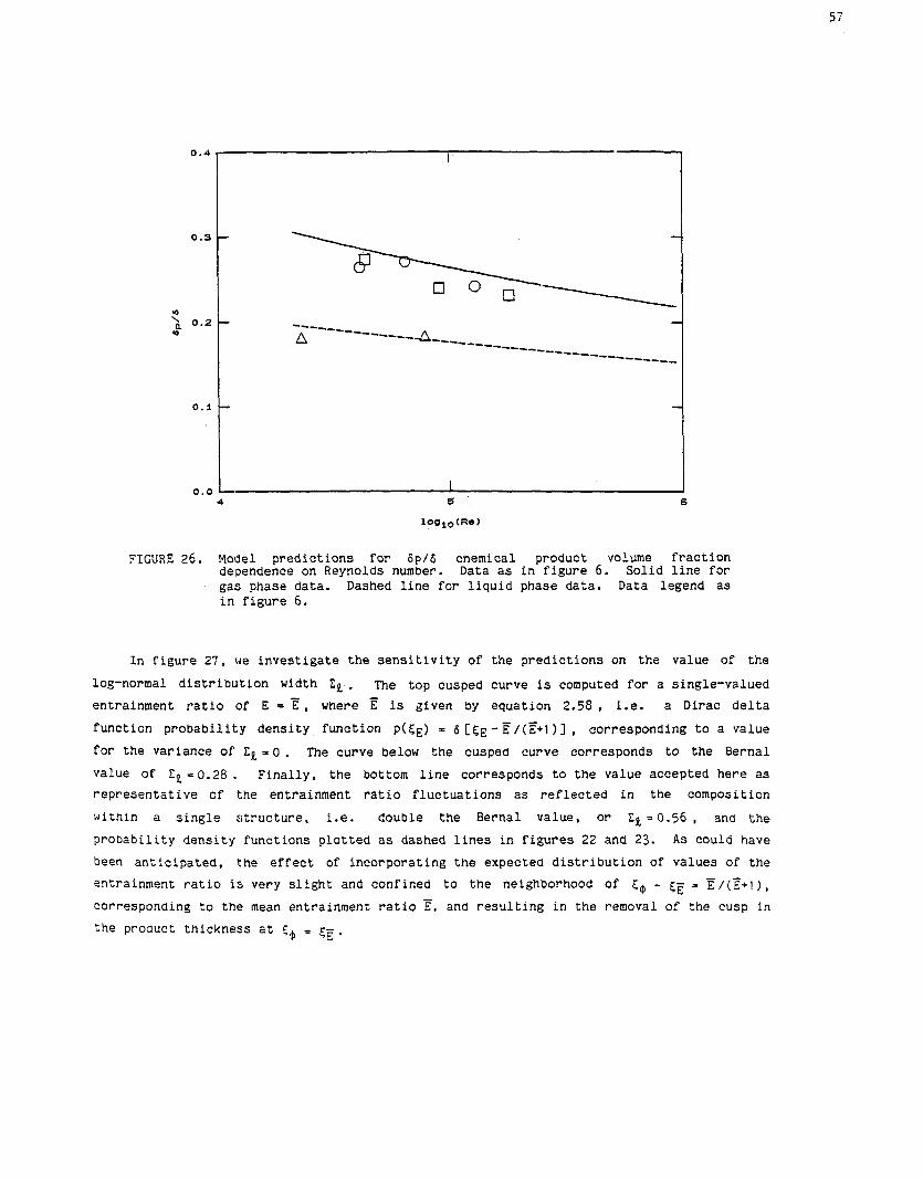
FIGURE 26. Model predictions for 6 p / 6 chemical product volume fraction dependence on Reynolds number. Data as in figure 6. Solid line for gas phase data. Dashed line for liquid phase data. Data legend as in figure 6.

In figure 27, we investigate the sensitivity of the predictions on the value of the

log-normal distribution width EII. The top cusped curve is computed for a single-valued

entrainment ratio of E = E, where F is given by equation 2.58, i.e. a Dirac delta

function probability density function p(tE) = G [ c E - F/ (E+l ) I , corresponding to a value for the variance of E L = O . The curve below the cusped curve corresponds to the Bernal

value of .IL = 0.28 . Finally, the bottom line corresponds to the value accepted here as

representative of t;he entrainment ratio fluctuations as reflected in the composition

within a single :itructure, i.e. double the Bernal value, or 2%=0.56, and the

probability density functions plotted as dashed lines in figures 22 and 23. AS could have

been anticipated, the effect of incorporating the expected distribution of values of the

entrainment ratio is very slight and confined to the neighborhood of 5 @ - 5~ = E / ( F + l ) , Corresponding to the mean entrainment ratio E, and resulting in the removal of the cusp in the product thickness at Eq = q.

FIGURE 27. Model s e n s i t i v i t y t o va lue of v a r i a n c e ZQ used i n entrainment mix tu re f r a c t i o n PDF. Corresponding p r e d i c t i o n s f o r 6 p ( 5 4 ) / 6 chemical product volume f r a c t i o n . Top ( cusped ) cu rve f o r ZQ , 0. Middle dashed curve f o r ZQ = 0 . 2 8 . Bottom ( s o l i d ) cu rve f o r ZQ = 0.56 used i n t h e model.

A s d i s c u s s e d e a r l i e r , t h e s e n s i t i v i t y of t h e computed v a l u e s of t h e product volume

f r a c t i o n t o t h e v a r i o u s c h o i c e s of t h e f low c o n s t a n t s is weak. By way o f example, t h e

Smooth c u r v e s i n f i g u r e s 4 and 5, which do n o t d i f f e r s u b s t a n t i a l l y from those i n f i g u r e s

24 and 25, were computed u s i n g a v a l u e of 8 = 5+ , l e a v i n g a l l o t h e r co l l s t an t s a t t h e i r

nominal va lues .

F i n a l l y , we n o t e t h a t t h e model p r e d i c t i o n s f o r t h e chemical product volume f r a c t i o n

t end t o be a l i t t l e h igh ( s e e f i g u r e 25 and 26 ) . One cou ld a rgue , con:j idering what is

being a t t empted h e r e w i t h a r a t h e r s i m p l e model and no a d j u s t a b l e paramtsters , t h a t t h e

agreement w i th exper iment is more than s a t i s f a c t o r y . We a l s o n o t e , however. t h a t two

assumpt ions t h a t were made i n t h e a n a l y s i s may no t be a d e q u a t e l y j u s t i f i e d i n t h e c a s e of

t h e hydrogen-f luor ine gas phase s h e a r l a y e r d a t a . One, as Broadwell 9r Mur~gal (1986) have

sugges t ed , t h e k i n e t i c s may no t be s u f f i c i e n t l y f a s t . If t h i s is indeed t h e c a s e , t h e

chemical product would be lower than would be observed i n t h e c a s e of i n f i n i t e k i n e t i c s .

Two, we r e c o g n i z e t h a t t h e assumpt ion o f equa l d i f f u s i v i t i e s f o r a l l t h e r e a c t a n t s p e c i e s

Such a va lue is, of c o u r s e , i n a d m i s s i b l e by v i r t u e of t h e bounds i n i n e q u a l i t y 2.25

is also not justified, hydrogen possessing a diffusivity roughly four times higher than

the other reactants/diluents in those experiments. It is difficult to give an a priori

assessment of the e~ffects of unequal diffusivities, possibly as coupled with the effects

of finite kinetics, at this time.

3.2 The mixed fluid fraction

An important quantity in turbulent mixing is the mixed fluid fraction within the

turbulent zone. It is to the mixing scalar (or scalar dissipation) field what

intermittency is to the turbulent velocity (or energy dissipation) field. Operationally,

it can be defined through the probability density function (PDF) of the conserved scalar,

i.e. ~ ( 5 1 , integrated across the shear layer width. In particular the quantity

for some small val.ue of 5, which excludes the unmixed fluid contributions from the

neighborhood of 5 - 0 and 5 - 1 , represents the volume fraction occupied by molecularly mixed fluid within the transverse extent of the turbulent shear layer. This quantity can

be expected to be a function of the fluid Schmidt number and the flow ~eynolds number (and

potentially also of the free stream density ratio and velocity ratio). In particular, we

would expect that an increase in the Schmidt number, at fixed Reynolds number, should

result in a decrease of 6,/6, which should vanish in the limit of infinite Schmidt

numbers. An a priori assessment of the behavior of the mixed fluid fraction at fixed

Schmidt number in the limit of very large Reynolds numbers cannot be made as readily and

will be discussed separately below.

While the integral indicated in equation 3.1 can, in principle, be estimated by

direct measurement of the scalar field S(:,t), and therefore also its PDF p(~) , it was pointed out by Breidenthal (1981) and Koochesfahani & Dimotakis (1986) that, as a

consequence of the inevitable experimental finite resolution difficulties at high Reynolds

numbers, such measur'ements will generally overestimate this quantity. It was also pointed

out in Koochesfaharii & Dimotakis, however, that reliable estimates are possible using the

results of chemica1l.y reacting experiments, namely the chemical product fractions 6p(~0)/6

and 6p(l-c0)/6 from a "flip" experiment conducted at a. and l/ao , for small values of $, , corresponding to a 5, = $,/ (l+$,) << 1 . In particular, the mixed fluid fraction can be

estimated in terms of the chemically reacting flow results by means of the relation

This is very close to the expression in equation 3.1 and equivalent to computing the

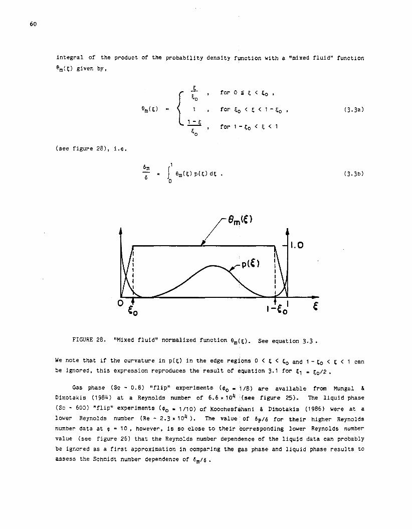
i n t e g r a l of t h e product of t h e p r o b a b i l i t y d e n s i t y f u n c t i o n wi th a "mixed f l u i d " f u n c t i o n

em(^) given by,

( s e e f i g u r e 281, i .e.

FIGURE 28. "Mixed f l u i d " normalized f u n c t i o n e m ( ( ) . See equa t ion 3 . 3 .

We n o t e t h a t i f t h e c u r v a t u r e i n p(E) i n t h e edge r e g i o n s 0 < 5 < Eo and ,I - c0 < 5 < 1 can

be ignored, t h i s e x p r e s s i o n r ep roduces t h e r e s u l t of equa t ion 3.1 f o r E l ,. c 0 / 2 .

Gas phase (Sc - 0.8) " f l i p " exper iments (fbo = 1 / 8 ) a r e a v a i l a b l e from Mungal &

Dimotakis ( 1 984) a t a Reynolds number of 6.6 x 104 ( s e e f i g u r e 25). The l i q u i d phase

(Sc - 600) " f l i p " exper iments (fbO - 1 /10) of Koochesfahani & Dimotakis (1986) were a t a

lower Reynolds number (Re - 2.3 x 1 o4 1. The value of 6p/6 f o r t h e i r h ighe r Reynolds

number d a t a a t @ = 1 0 , however, is s o c l o s e t o t h e i r corresponding lower Reynolds number

va lue ( s e e f i g u r e 26) t h a t t h e Reynolds number dependence o f t h e l i q u i d d a t a can probably

be ignored a s a f i r s t approximat ion i n comparing t h e gas phase and l i q u i d phase r e s u l t s t o

a s s e s s t h e Schmidt number dependence of 6,/6 .

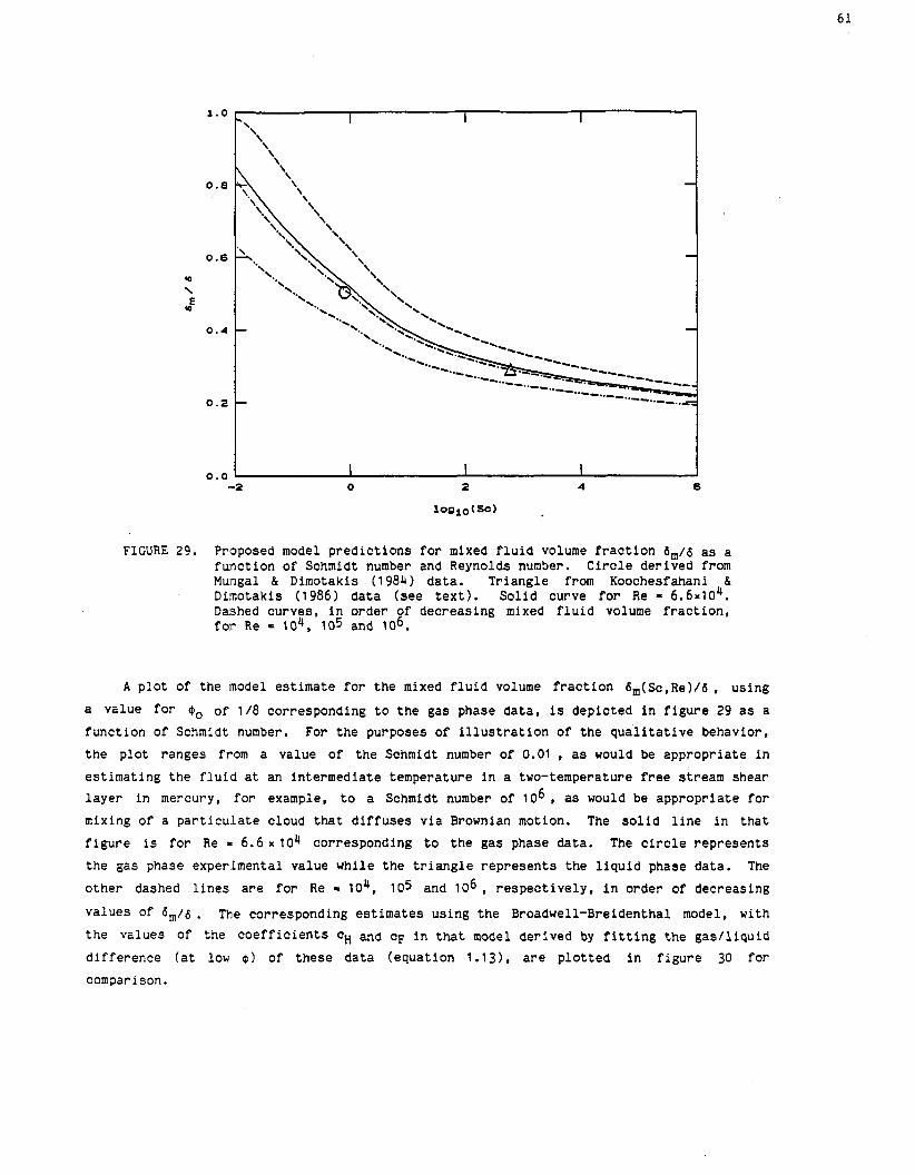
FIGURE 29. Proposed model predictions for mixed fluid volume fraction 6,/6 as a function of Schmidt number and Reynolds number. Circle derived from Mulngal & Dimotakis (1984) data. Triangle from Koochesfahani & Dilnotakis (1986) data (see text). Solid curve for Re = 6.6x104. Dashed curves, in order of decreasing mixed fluid volume fraction, for Re = 104, 105 and lo6.

A plot of the lnodel estimate for the mixed fluid volume fraction bm(Sc,Re)/6, using

a value for $, of 1/8 corresponding to the gas phase data, is depicted in figure 29 as a

function of Schmidt number. For the purposes of illustration of the qualitative behavior,

the plot ranges from a value of the Schmidt number of 0.01 , as would be appropriate in estimating the fluid at an intermediate temperature in a two-temperature free stream shear

layer in mercury, for example, to a Schmidt number of lo6, as would be appropriate for

mixing of a particu.late cloud that diffuses via Brownian motion. The solid line in that

figure is for Re m 6.6 x 104 corresponding to the gas phase data. The circle represents

the gas phase experimental value while the triangle represents the liquid phase data. The

other dashed lines are for Re - lo4, 105 and lo6 , respectively, in order of decreasing values of 6,/6 . The corresponding estimates using the Broadwell-Breidenthal model, with

the values of the coefficients CH and CF in that model derived by fitting the gaslliquid

difference (at low @ ) of these data (equation 1.131, are plotted in figure 30 for

comparison.

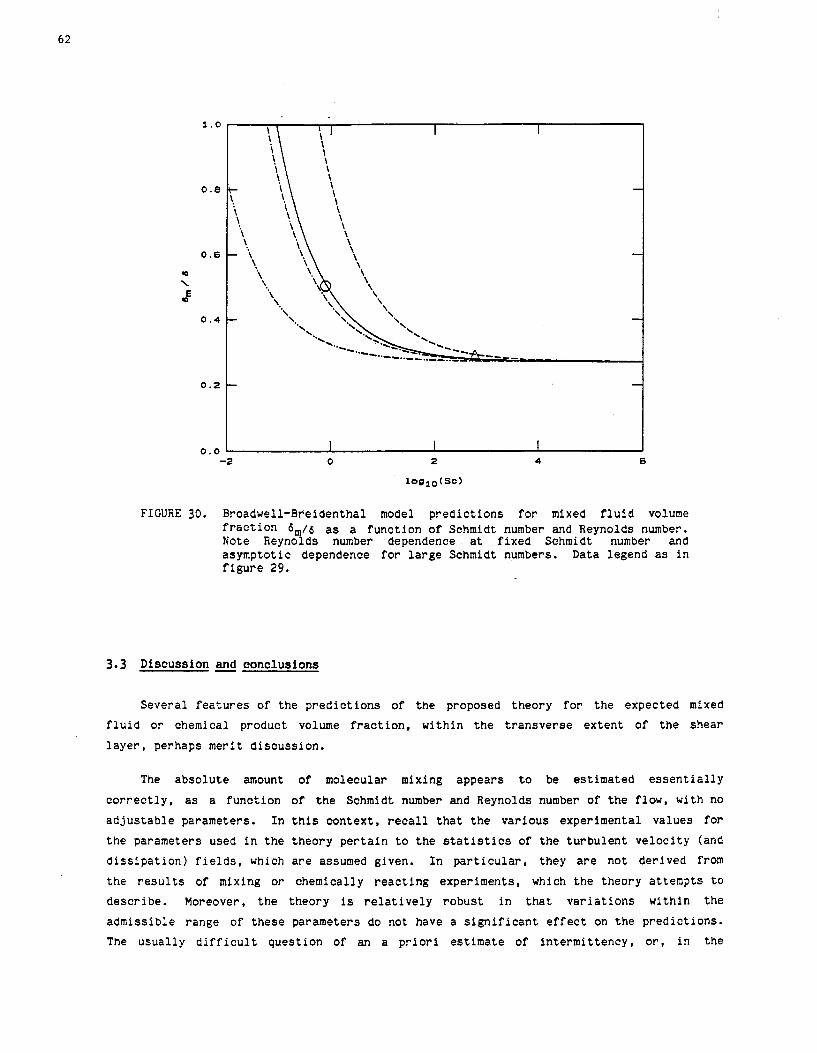
FIGURE 30. Broadwell-Breidenthal model p r e d i c t i o n s f o r mixed f l u i d volume f r a c t i o n 6,/6 a s a f u n c t i o n o f Schmidt number and Reyncllds number. Note Reynolds number dependence a t f i x e d Schmidt number and a sympto t i c dependence f o r l a r g e Schmidt numbers. Data legend a s i n f i g u r e 29.

3.3 Discuss ion and c o n c l u s i o n s

Seve ra l f e a t u r e s of t h e p r e d i c t i o n s of t h e proposed t h e o r y f o r the! expected mixed

f l u i d o r chemical product volume f r a c t i o n , w i t h i n t h e t r a n s v e r s e e x t e n t of t h e s h e a r

l a y e r , perhaps merit d i s c u s s i o n .

The a b s o l u t e amount of molecular mixing appea r s t o be e s t ima ted e s s e n t i a l l y

c o r r e c t l y , as a f u n c t i o n o f t h e Schmidt number and Reynolds number of t,he f low, wi th no

a d j u s t a b l e parameters . I n t h i s c o n t e x t , r e c a l l t h a t t h e v a r i o u s expe r imen ta l v a l u e s f o r

t h e parameters used i n t h e t h e o r y p e r t a i n t o t h e s t a t i s t i c s of t h e turbulcrnt v e l o c i t y (and

d i s s i p a t i o n ) f i e l d s , which a r e assumed given. I n p a r t i c u l a r , t hey a r e n o t de r ived from

t h e r e s u l t s of mixing o r chemical ly r e a c t i n g exper iments , which t h e theo ry a t t e m p t s t o

d e s c r i b e . Moreover, t h e theo ry is r e l a t i v e l y r o b u s t i n t h a t v a r i a t i o n s w i t h i n t h e

a d m i s s i b l e range o f t h e s e parameters do no t have a s i g n i f i c a n t e f f e c t on t h e p r e d i c t i o n s .

The u s u a l l y d i f f i c u l t ques t ion o f an a p r i o r i e s t i m a t e of i n t e r m i t t e n c y , o r , i n t h e

p r e s e n t c o n t e x t , o f t h e volume f r a c t i o n i n t h e f low occupied by unmixed ( u n r e a c t e d ) f l u i d ,

is addres sed through t h e no rma l i za t ion of t h e vo lume- f i l l i ng spec t rum of s c a l e s . F i n a l l y ,

e x c e p t f o r s w i t c h i n g (matched) a n a l y t i c a l e x p r e s s i o n s , depending on t h e r e l a t i v e

magnitudes of t h e v a r i o u s ( i n n e r ) s c a l e s of t h e problem, i . e . A D , A H , A c , l i q u i d s and

g a s e s a r e t r e a t e d i n a u n i f i e d way through t h e e x p l i c i t dependence of t h e r e s u l t s on

Schmidt number.

The theo ry a l s ~ o p r e d i c t s t h a t , a t s u f f i c i e n t l y h igh Reynolds numbers, t h e amount of

mixed f l u i d o r che!mical product i n a g a s phase s h e a r l a y e r would be less than what would

be observed i n a l i q u i d l a y e r a t s u f f i c i e n t l y low Reynolds numbers ( r e c a l l f i g u r e 29). I n

f a c t , t h e i n t e r e s t i n g and c o n t r o v e r s i a l p r e d i c t i o n is t h a t t h e volume f r a c t i o n of t h e

mixed f l u i d t e n d s t o z e r o wi th i n c r e a s i n g Reynolds number, a l b e i t s l owly , p o s s e s s i n g no

Reynolds number independent a sympto t i c (non-zero) va lue . One might i n t u i t i v e l y a rgue t h a t

a s t h e Reynolds number i n c r e a s e s , t h e i n t e r f a c i a l s u r f a c e a r e a a v a i l a b l e f o r mixing must

i n c r e a s e (under tlhe a c t i o n of t h e h ighe r s u s t a i n a b l e s t r a i n r a t e s i n t h e f l ow) and

t h e r e f o r e a l s o t h e mixing r a t e . T h i s argument, however, is incomple te i n t h a t i t f a i l s t o

r e c o g n i z e t h a t t h e t h i c k n e s s of t h e mixed f l u i d l a y e r s t r a d d l i n g t h e i n t e r f a c e must be

d e c r e a s i n g , i n f a c t , approximate ly i n v e r s e l y a s t h e i n t e r f a c e a r e a is i n c r e a s i n g , by t h e

f o r c e of t h e same arguments. Consequent ly , t h e s e two e f f e c t s must approximate ly c a n c e l

each q t h e r . I n p a r t i c u l a r , t h e model p r e d i c t s t h a t a s t h e Reynolds number i n c r e a s e s , t h e

a s s o c i a t e d diffusedl l a y e r t h i c k n e s s must be d e c r e a s i n g a t a s l i g h t l y f a s t e r r a t e , s i n c e

t h e f low volume f r a c t i o n occupied by t h e mixed f l u i d is d e c r e a s i n g ( s l o w l y ) w i th

i n c r e a s i n g Reynolds number. Th i s behavior is co r robora t ed by t h e l i m i t e d d a t a a v a i l a b l e ,

which i n d i c a t e a n lonotonica l ly d e c r e a s i n g volume f r a c t i o n of chemical product wi th

i n c r e a s i n g Reynolds number, i n good q u a n t i t a t i v e agreement w i th t h e p r e d i c t e d Reynolds

number dependence.

It should be noted t h a t t h e p r e d i c t i o n is not t h a t mixing c e a s e s i n t h e l i m i t o f

i n f i n i t e Reynolds :numbers. I f one were t o i n c r e a s e t h e Reynolds number by i n c r e a s i n g t h e

downstream coordina ' te x , f o r example, t h e i n t e g r a t e d mixed f l u i d t h i c k n e s s 6 m ( ~ ) would

i n c r e a s e a lmost p ro :po r t i ona l ly t o t h e s h e a r l a y e r t h i c k n e s s & ( X I , s p e c i f i c a l l y

Consequent ly , however, t h e mixed f l u i d volume f r a c t i o n would d e c r e a s e l o g a r i t h m i c a l l y , o r

i n t e rms of t h e Reylnolds number,

This r e s u l t is a d i r e c t consequence of t h e assumed s t a t i s t i c a l Weight and

normal izat ion over t h e range of s c a l e s of the problem. I n p a r t i c u l a r , accep t ing t h e

W ( A ) dA - dA/A s t a t i s t i c a l weight f o r t h e moment, t h e dependence on th.e l o c a l Reynolds

number e n t e r s through t h e r a t i o of the o u t e r l a r g e s c a l e 6 t o t h e inner s c a l e

A c = 03/2 A K , where 0 = 3 and A K is t h e Kolmogorov s c a l e , i . e .

and where t h e subsc r ip ted a n g l e b racke t s denote t h e ensemble average over t h e f l u c t u a t i o n s

i n t h e l o c a l d i s s i p a t i o n r a t e E . We no te t h a t , aga in accep t ing t h e W ( A ) dA - dA/A

s t a t i s t i c a l weight, a non-zero asymptot ic value f o r 6,/6 a t h igh Reynolds numbers would be

t h e p r e d i c t i o n only i f < ln(6/AK) > € + c o n s t a n t , a s Re + m .

We have examples of such behavior i n high Reynolds number t u r b u l e n t f lows. I n

p a r t i c u l a r , t h e s k i n f r i c t i o n c o e f f i c i e n t f o r a t u r b u l e n t boundary l a y e r over a (smooth)

f l a t P l a t e a t high Reynolds number appears t o decrease approximately logiar i thmical ly wi th

Reynolds number. For s i m i l a r r easons , t h e p ressure g r a d i e n t c o e f f i c i e n t f o r t u r b u l e n t

(smooth w a l l ) p ipe flow a l s o decreases l o g a r i t h m i c a l l y wi th Reynolds number. It is

i n t e r e s t i n g t o no te , however, t h a t i n t h e s e examples t h e behavior w i l l asymptote t o a

Reynolds number independent regime, i f t h e wal l cannot be considered .smooth compared t o

t h e Smal les t Sca les t h e tu rbu lence can s u s t a i n and i n t e r f e r e s with t h e i r p a r t i c i p a t i o n i n

t h e dynamics, i . e . i f a Reynolds number independent minimum s c a l e is imposed on t h e

dynamics of t h e flow. Analogously, i n my opinion, t h e assignment of an Eu le r i an , Reynolds

number independent volume f r a c t i o n occupied by t h e homogeneously mixed f l u i d i n t h e

Broadwell-Breidenthal model l e a d s pe r fo rce t o a Reynolds number independent mixed f l u i d

(and chemical product) volume f r a c t i o n i n t h e l i m i t of l a r g e Reynolds numbers. I n a f r e e

shea r l a y e r , however, i n which t h e tu rbu lence does not have t o contend wi th any i n t r u d i n g

rough w a l l s o r e x t e r n a l l y imposed minimum s c a l e s , t h e flow w i l l genera te its minimum

( d i s s i p a t i o n / d i f f u s i o n ) s c a l e s , of ever dec reas ing s i z e a s t h e Reynolds number i n c r e a s e s ,

and which w i l l p a r t i c i p a t e i n t h e mixing and d i s s i p a t i o n dynamics unimpeded.

We recogn ize , however, t h a t t h e Broadwell-Breidenthal argument is not Euler ian .

These au thors i n t e g r a t e d t h e cascade t ime s c a l e a s s o c i a t e d wi th each s c a l e A and concluded

t h a t t h e Lagrangian t ime t o cascade t o t h e Kolmogorov s c a l e becomes independent of the

Reynolds number a t high Reynolds numbers. This is a c e n t r a l idea i n t h e

Broadwell-Breidenthal model. If one a c c e p t s it, one must a l s o accep t t h a t f l u i d en t ra ined

a t an upstream s t a t i o n xl cascades t o t h e d i f f u s i o n (Kolmogorov) s c a l e by a s t a t i o n X K ,

such t h a t x ~ / x l is independent of t h e Reynolds number. The argument is important and, if

Cor rec t , d i f f i c u l t t o r e c o n c i l e with t h e proposed p red ic ted shea r l a y e r mixing behavior a t

h igh Reynolds numbers.

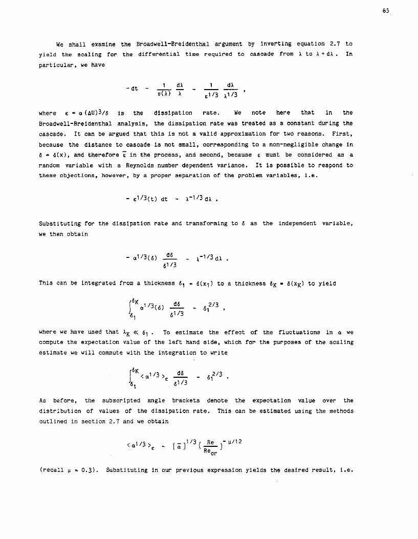
We shall examine the Broadwell-Breidenthal argument by inverting equation 2.7 to

yield the scaling for the differential time required to cascade from X to X + d X . In

particular, we have

where E = a (~~)3/6 is the dissipation rate. We note here that in the

Broadwell-Breidenthal analysis, the dissipation rate was treated as a constant during the

cascade. It can be argued that this is not a valid approximation for two reasons. First,

because the distance to cascade is not small, corresponding to a non-negligible change in

6 = 6(x), and therefore 7 in the process, and second, because E must be considered as a

random variable with a Reynolds number dependent variance. It is possible to respond to

these objections, however, by a proper separation of the problem variables, i.e.

Substituting for the dissipation rate and transforming to 6 as the independent variable,

we then obtain

This can be integrated from a thickness = 6(x1) to a thickness tiK = 6(xK) to yield

where we have used that XK << 61 . To estimate the effect of the fluctuations in a we

compute the expectation value of the left hand side, which for the purposes of the scaling

estimate we will commute with the integration to write

As before, the subscripted angle brackets denote the expectation value over the

distribution of values of the dissipation rate. This can be estimated using the methods

outlined in section 2.7 and we obtain

(recall u = 0.3). Substituting in our previous expression yields the desired result, i.e.

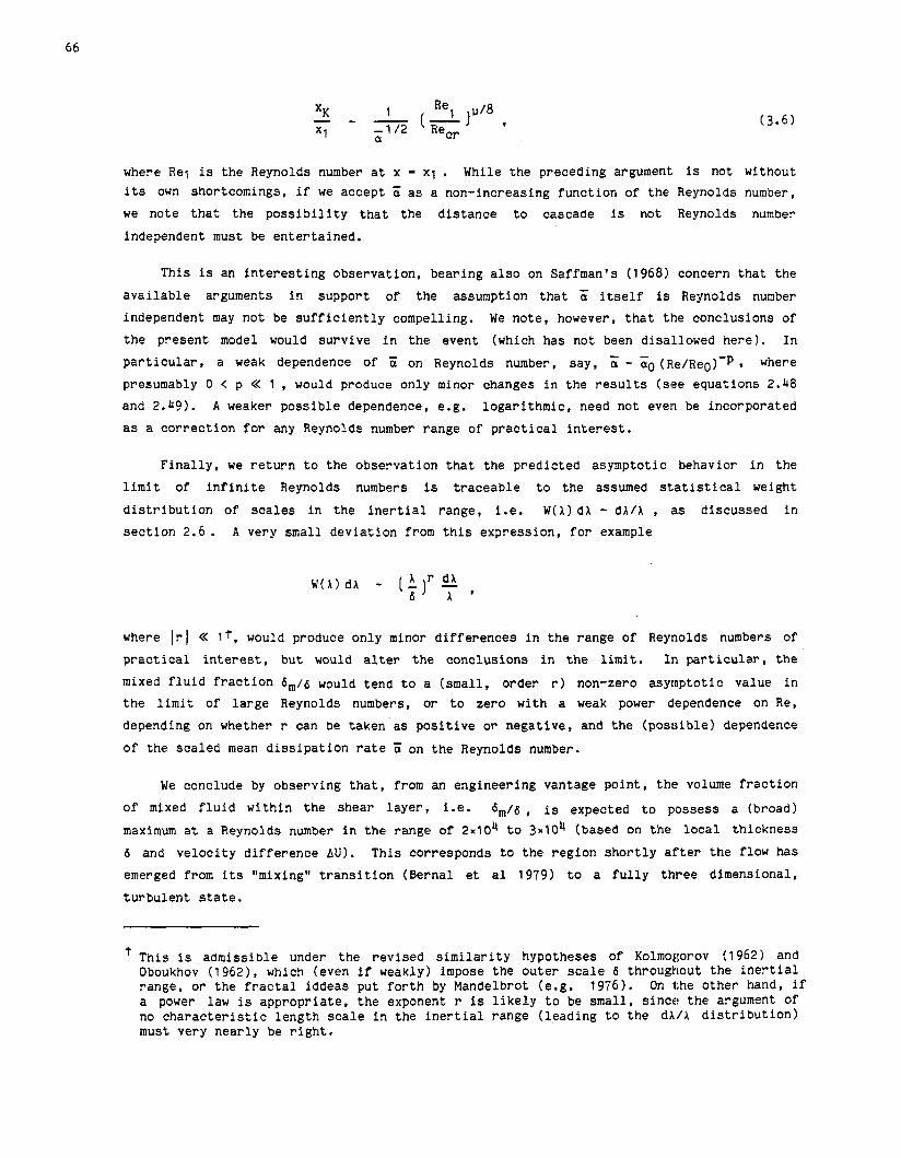
where Re1 is the Reynolds number at x = xi . While the preceding argument is not without its own shortcomings, if we accept a as a non-increasing function of the Reynolds number, we note that the possibility that the distance to cascade is not Reynolds number

independent must be entertained.

This is an interesting observation, bearing also on Saffman's (1968) concern that the

available arguments in support of the assumption that a itself is Reynolds number independent may not be sufficiently compelling. We note, however, that the conclusions of

the present model would survive in the event (which has not been disallowed here). In - - particular, a weak dependence of a on Reynolds number, say, a - a0 (~le/~e~)-P , where presumably 0 < p << 1 , would produce only minor changes in the results (see equations 2.48 and 2.49). A weaker possible dependence, e.g. logarithmic, need not even be incorporated

as a correction for any Reynolds number range of practical interest.

Finally, we return to the observation that the predicted asymptotic behavior in the

limit of infinite Reynolds numbers is traceable to the assumed st.atistica1 weight

distribution of scales in the inertial range, i.e. W(A)dA - dA/A , as discussed in

section 2.6. A very small deviation from this expression, for example

where Irl << It, would produce only minor differences in the range of Reynolds numbers of

practical interest, but would alter the conclusions in the limit. In particular, the

mixed fluid fraction 6,/6 would tend to a (small, order r) non-zero asymptotic value in

the limit of large Reynolds numbers, or to zero with a weak power dependence on Re,

depending on whether r can be taken as positive or negative, and the (possible) dependence

of the scaled mean dissipation rate E on the Reynolds number.

We conclude by observing that, from an engineering vantage point, tht? volume fraction

of mixed fluid within the shear layer, i.e. 6,/6, is expected to possess a (broad)

maximum at a Reynolds number in the range of 2x10~ to 3x104 (based on the local thickness

6 and velocity difference AU). This corresponds to the region shortly arter the flow has

emerged from its "mixing" transition (Bernal et a1 1979) to a fully three dimensional,

turbulent state.

This is admissible under the revised similarity hypotheses of Ko1mo~:orov (1962) and Oboukhov (1962), which (even if weakly) impose the outer scale 6 throughout the inertial range, or the fractal iddeas put forth by Mandelbrot (e.g. 1976). On the other hand, if a power law is appropriate, the exponent r is likely to be small, since? the argument of no characteristic length scale in the inertial range (leading to the dA/A distribution) must very nearly be right.

ACKNOWLEDGEMENTS

I would l i k e t o acknowledge t h e many d i s c u s s i o n s w i t h i n t h e GALCIT community, which

d i r e c t l y or i n d i r e c t l y have c o n t r i b u t e d t o t h i s paper. Without wishing t o imply

endorsement, I wou.ld s p e c i f i c a l l y l i k e t o r e c o g n i z e t h e d i s c u s s i o n s w i th D r . J.

Broadwell , P ro f . R. Narasimha and P ro f . P. Saffman. A d d i t i o n a l l y , t h e c r i t i ca l

comments by P ro f . A. Leonard and Mr. P. Miller c o n t r i b u t e d t o many impor tant

improvements and c . L a r i f i c a t i o n s i n t h e f i n a l form of t h e t e x t . F i n a l l y , I would l i k e t o

thank Mr. C . F r i e l e r f o r per forming t h e numer ica l i n t e g r a t i o n o f t h e d i f f e r e n t i a l

e q u a t i o n f o r t h e ve . l oc i ty c o r r e l a t i o n f u n c t i o n h ( c ) i n s e c t i o n 2 . 6 .

T h i s work is p a r t of a l a r g e r e f f o r t t o i n v e s t i g a t e mixing and combustion i n

t u r b u l e n t s h e a r f l ows , sponsored by t h e A i r Force O f f i c e o f S c i e n t i f i c Research Con t r ac t

No. F49620-79-C-0'159 and Grant No. AFOSR-83-0213, whose suppor t is g r a t e f u l l y

acknowledged.

REFERENCES

ASHURST, W. T., KEIRSTEIN, A. R . , KERR, R. M. and GIBSON, C. H. . [ I9871 "Alignment of V o r t i c i t y and S c a l a r Gradient w i th S t r a i n Rate i n Simula ted Navier-Stokes Turbulence", Pllys. F l u i d s 30( 81, 2343-2353.

BATCHELOR, G. K . [ I9591 l lSmall-scale v a r i a t i o n o f convected q u a n t i t i e s l i k e t empera tu re i n t u r b u l e n t f l u i d . P a r t I. Genera l d i s c u s s i o n and t h e c a s e of small c o n d u c t i v i t y " , J. F l u i d Mech. 5, 113-133. - --- -

BATCHELOR, G. K., IHOWELLS, I. D. and TOWNSEND, A. A. [ l 9591 "Small-scale v a r i a t i o n o f convected q u a n t i t i e s l i k e t empera tu re i n t u r b u l e n t f l u i d . P a r t 2. The case o f l a r g e c o n d ~ c t i v i t y ~ ~ , J, Fluid Mech. 5, 134-139.

BERNAL, L. P. , BREI:DENTHAL, R. E., BROWN, G. L. , KONRAD, J. H. and ROSHKO. A. C19791 "On t h e Developmen~t of Three Dimensional Smal l S c a l e s i n Turbu len t Mixing Layers." , 2nd Symposium on Turbu len t Shear Flows, 2-4 J u l y 1979, Imper i a l Co l l ege , England.

BETCHOV, R. [1977] I f T r a n s i t i o n w , Handbook of Turbulence [ (Ed. W. F r o s t and T. H. Moulden, Plenum P r e s s ) , 147-164.

BETCHOV, R. and SZEWCZYK, A. [ I9631 " S t a b i l i t y of a s h e a r l a y e r between p a r a l l e l streams", Phys. F l u i d s 6 , 1391-96.

BILGER, R . W. [ I 9801 "Turbulent Flows wi th Nonpremixed Reactants1 ' , Turbulent React ing Flows (Sp r inge r -Ver l ag , Topics 2 Applied Phys i c s 44, 1980, Ed. P. A. Libby, F. A. Wi l l i ams) , 65-1 13.

BREIDENTHAL, R . E. [19811 l l S t r u c t u r e i n Turbu len t Mixing Layers and Wakes Using a Chemical Reaction", J, Flu id Mech. 2, 1-24.

BROADWELL, J. E. and BREIDENTHAL, R. E. 119821 "A Simple Model of Mixing and Chemical React ion i n a Turbulent Shear Layer", J, Flu id Mech. 125, 397-410.

BROADWELL, J. E. and DIMOTAKIS, P. E. [19863 implications of Recent Exper imenta l R e s u l t s f o r Modeling React ions i n Turbulent Flows", A I A A J. 2 4 ( 6 ) , 885-889.

BROADWELL, J. E. and MUNGAL, M. G. [ I9861 "The e f f e c t s o f ~ a m k s h l e r number i n a t u r b u l e n t s h e a r l a y e r u , GALCIT Report FM86-01.

BROWN, G. L. and REBOLLO, M. R . [ I9721 "A Smal l , Fast-Response Probe t o Measure Composition o f a Binary Gas Mixture", A I A A J. 1 0 ( 5 ) , 649-652.

BROWN, G. L. and ROSHKO, A. [ I9741 "On Dens i ty E f f e c t s and Large S t r u c t u r e i n Turbulent Mixing Layers", J, Flu id Mech. 6 4 ( 4 ) , 775-81 6.

DIMOTAKIS, P. E. [I 9861 llTwo-Dimensional Shear-Layer Entra inmentw, l* J, 24 ( 1 1 1, 1791 -1 796.

DIMOTAKIS , P. E. and BROWN, G. L. [I9761 "The Mixing Layer a t High Reynolds Number: Large-St ructure Dynamics and Entrainment1!, J, Flu id Mech. 7 8 ( 3 ) , 535-560 + 2 p l a t e s .

FIEDLER, H. Z'. [ I9751 "On Turbulence S t r u c t u r e and Mixing Mechanism i n F ree Turbulent Shear Flowsv, from: (S. N. B. Murthy, Ed.) Turbulent Mixin8 2 Non-Reactive and Reac t ive Flows (Plenum P r e s s 1, 381 -409.

GIBSON, C. H. [ I9681 "Fine S t r u c t u r e of S c a l a r F i e l d s Mixed by 'Turbulence. 11. S p e c t r a l Theory", Phys. F l u i d s 1 1 ( 1 1 ) , 2316-2327.

G U R V I C H , A. S. and YAGLOM, A. M. [ I9671 "Breakdown o f Eddies and P r o b a b i l i t y D i s t r i b u t i o n s f o r Small S c a l e Turbulenceqq, Phys. F l u i d s (1967 Sup. ) , 59-65.

HERMANSON, J. C . , MUNGAL, M. G. and DIMOTAKIS, P. E. [ I 9871 "Heat Release E f f e c t s on Shear Layer Growth and Entra inmentw, A I A A J. 2 5 ( 4 ) , 578-583.

KERR, R. M. [ I 9853 "Higher-order d e r i v a t i v e c o r r e l a t i o n s and t h e a l ignement of sma l l - sca l e s t r u c t u r e s i n i s o t r o p i c numer ica l t u r b u l e n c e n , J, F l u i d Mech. 153, 31 -58.

KOLLMAN, W. [ I 9841 " P r e d i c t i o n o f i n t e r m i t t e n c y f a c t o r f o r t u r b u l e n t s h e a r f lows", J. 2 2 ( 4 ) , 486-492. - -

KOLLMANN, W. and JANICKA, J . [1982] "The P r o b a b i l i t y Dens i ty Funct ion of a Pass ive S c a l a r i n Turbulent Shear Flowsw, Phys. F l u i d s 25, 1755-1769.

KOLMOGOROV, A. N. [ I9411 "Local s t r u c t u r e of t u rbu lence i n an incompress ib l e v i s c o u s f l r l i d a t very h igh Reynolds numbersq1, Dokl. Akad. Nauk SSSR 30, 299, r e p r i n t e d i n Usp. Fiz . Nauk 93, 476-481 (19671, t r a n s l . i n Sov. Phys. Usp. 1 0 ( 6 ) , 734-736 (1968)-

KOLMOCOROV, A. N. [I9621 "A r e f inemen t o f p rev ious hypotheses concerning t h e l o c a l s t r u c t u r e of t u r b u l e n c e i n a v i s c o u s incompress ib l e f l u i d a t h igh ]Reynolds numberq', J. F lu id Mech 13 , 82-85. - ---

KONRAD, J. H. [ I9761 &I Experimental I n v e s t i g a t i o n of Mixing & Two-Dimensional Turbulent Shea r Flows wi th App l i ca t ions Diffusion-Limited Chelmical React ions , Ph.D. T h e s i s , C a l i f o r n i a I n s t i t u t e of Technology, and P r o j e c t SQUID Technica l Report CIT-8-PU (December 1976) .

KOOCHESFAHANI, M. M. and DIMOTAKIS, P. E. [1986] "Mixing and chemical r e a c t i o n s i n a t u r b u l e n t l i q u i d mixing l a y e r w , J, Flu id Mech. 170, 83-112.

LUNDGREN, T. S. [1982] "S t r a ined S p i r a l Vor tex Model f o r Turbu len t F ine S t r u c t u r e f 1 , Phys. F l u i d s 2 5 ( 1 2 ) , 21 93-2203.

LUNDGREN, T. S. [ I9851 "The c o n c e n t r a t i o n Spectrum of t h e p roduc t of a f a s t b imolecular r e a c t i o n " , Chem. Eng. Sc. 4 0 ( 9 ) , 1641 -1652.

MANDELBROT, B. [I 9'763 I t I n t e r m i t t e n t t u r b u l e n c e and f r a c t a l dimension: k u r t o s i s and t h e s p e c t r a l expon'ent 5 /3 + Bv, Turbulence and t h e Navier S tokes Equat ions (Conf. Proc. , U . Paris-Sud, Orsay, 12-13 June 1975, Publ: Lec tu re Notes 2 Mathematics 565, Ed. A. Dold, B. Eckmann, Spr inger-Ver lag) , 121 -1 45.

MARBLE, F. E. and BROADWELL, J. E. [1977] "The cohe ren t f lame model f o r t u r b u l e n t chemical r e a c t i o n s f f , P r o j e c t SQUID Techn ica l Report TRW-9-PU.

M O N I N , A. S. and YACLOM, A. M. El9751 S t a t i s t i c a l F l u i d Mechanics: Mechanics of Turbulence 2 ( )Engl ish t r a n s l a t i o n o f t h e 1965 Russ ian t e x t . Ed. J. L. Lumley, MIT P r e s s ) .

MUMGAL, M. G. and DIMOTAKIS, P. E. [ I 9841 "Mixing and combustion wi th low hea t release i n a t u r b u l e n t mixing l a y e r w , Jr F l u i d Mech. 148, 349-382.

MUNGAL, M. G , HERMAIVSON, J. C. and DIMOTAKIS, P. E. [I 9851 "Reynolds Number E f f e c t s on Mixing and Combustion i n a Reac t ing Shear Laye rv , A I A A J. 23( 91, 141 8-1 423.

N O V I K O V , E. A. [1!361 I "Energy Spectrum of an Incompres s ib l e F l u i d i n Turbu len t Flow", Repor ts Ac. :k. USSR 1 3 9 ( 2 ) , 331-334, t r a n s l a t e d i n Sov. Phys. Doklady 6 ( 7 ) , 571 -573 (1 962):-

OBOUKHOV, A. M. ['1962] "Some s p e c i f i c f e a t u r e s of a tmosphe r i c t u rbu lence" , Jr F l u i d Mech. 1 3 , 77-81 . - -

POPE, S. B. [1985:] "PDF Methods f o r Turbu len t Reac t ive Flows", Prog. Energy Comb. Sc. 11 119-192. -'

ROGERS, M. M . , MOII?, P. and REYNOLDS, W. C. [I 9861 "The S t r u c t u r e and Modeling o f t h e Hydrodynamic and Pas s ive S c a l a r F i e l d s i n Homogeneous Turbu len t Shear Flow", S t a n f o r d U n i v e r s i t y Report TF-25.

ROSHKO, A . [1976] q lS t ruc tu re o f Turbu len t Shea r Flows: A New Look", AIAA J, 14, 1349-1 357, and 15, 768.

SAFFMAN, P. G. [I51681 Topics i n Non-Linear Phys i c s (Ed. N. Zabusky, Spr inger-Ver lag , B e r l i n ) , 485-614.

SPENCER, B. W. and JONES, B. G. [1971] f f S t a t i s t i c a l I n v e s t i g a t i o n o f P r e s s u r e and V e l o c i t y F i e l d s i n t h e Turbulent Two St ream Mixing Layer1?, A I A A Paper NO. 71-613.

SREENIUASAN, K. R . , TAVOULARIS, S. and CORRSIN, S. [ I9811 n A Tes t of Grad ien t T ranspor t and i ts G e n e r a l i z a t i o n s w , 3 rd I n t e r n a t i o n a l Symposium on Turbu len t Shear Flows, U. C . Davis , 9-1 1 September 1 981 (Pub l i shed by Spr inger-Ver lag 1982, Eds. Bradbury, L. J. S., Dur s t , F., Launder, B. E., Schmidt , F. W. and Whitelaw, J. H. Turbulent Shear Flows 21, 96-1 12. --

TENNEKES, H. and LLIMLEY, J. L. 119721 A F i r s t Course i n Turbulence (MIT P r e s s ) .

TOWNSEND, A. A. 11951 I "On t h e f i n e s t r u c t u r e o f t u r b u l e n c e w Proc. Roy. Sot. A 208, 534-542.

VAN ATTA, C. W . artd ANTONIA, R. A. [ I9801 "Reynolds number dependence of skewness and f l a t n e s s f a c t o r s of v e l o c i t y d e r i v a t i v e s " , Phys. F l u i d s 2 3 ( 2 ) , 252-257.

WYGNANSKI, I. and E'IEDLER, H. E. [ I 9701 "The Two Dimensional Mixing Region", J- Flu id Mech. 41 (21 , 327-361 . --