Turbulent boundary layer

0. Are they so different from laminar flows ?1. Three main effects of a solid wall2. Statistical description: equations & results3. Mean velocity field: classical asymptotic theory4. Rugosity5. Coherent structures & turbulence dynamics6. Turbulent drag: generation & control

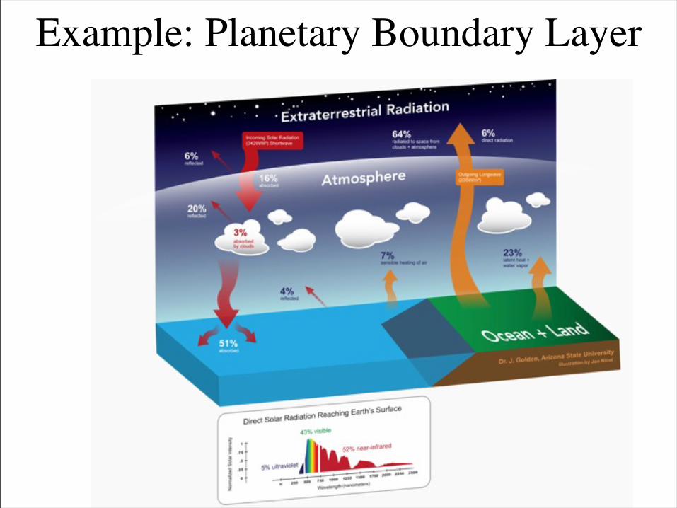
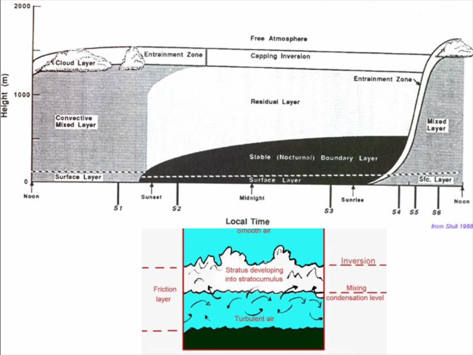
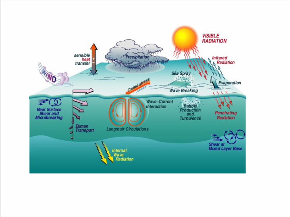
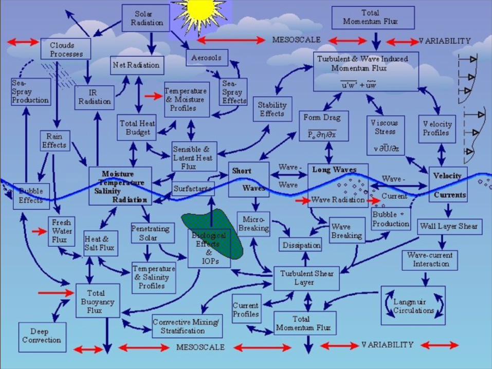
Example: Planetary Boundary Layer

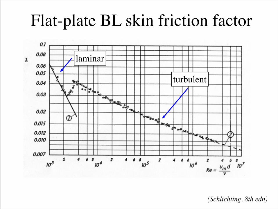
Flat-plate BL skin friction factor

(Schlichting, 8th edn)

laminar

turbulent

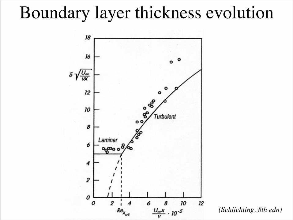
Boundary layer thickness evolution

(Schlichting, 8th edn)

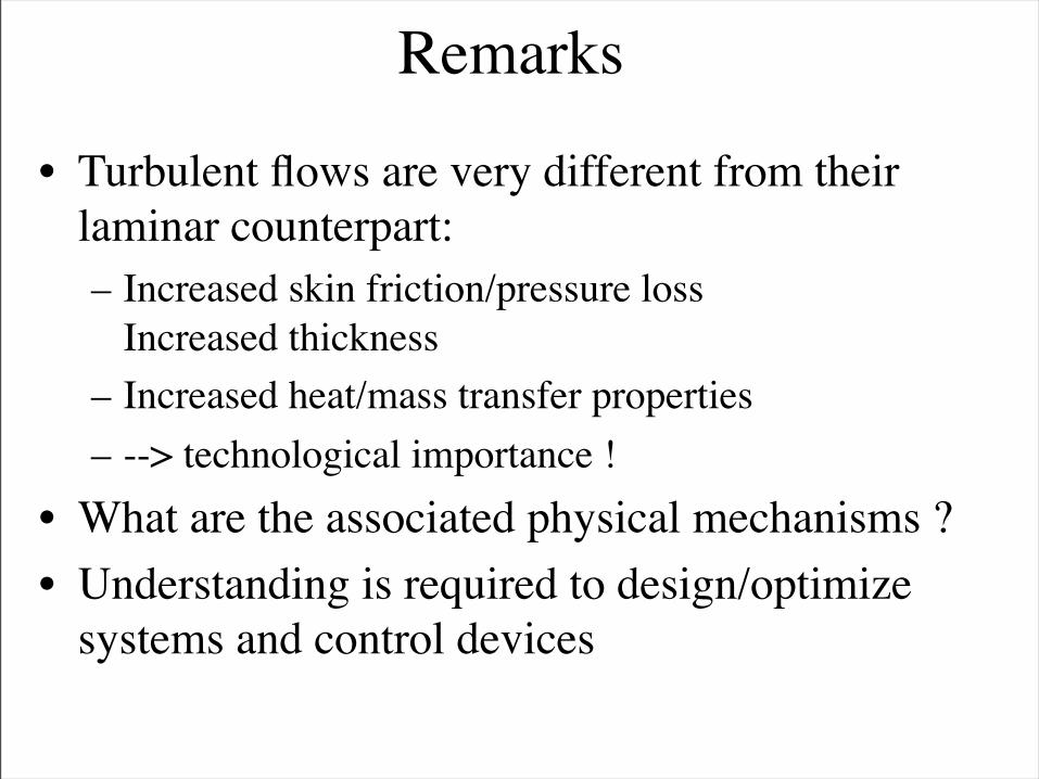
Remarks

• Turbulent flows are very different from their laminar counterpart:– Increased skin friction/pressure loss

Increased thickness– Increased heat/mass transfer properties– --> technological importance !

• What are the associated physical mechanisms ?• Understanding is required to design/optimize

systems and control devices

The three effects of a solid wall

• Hypotheses about the solid surface:– Impermeable– Infinitely rigid– Plane– Non-reactive, cold– No-slip boundary condition holds (beware of

micro/nano-channel dynamics !)

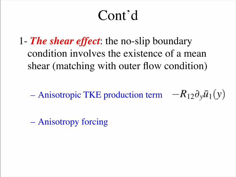
Cont’d1- The shear effect: the no-slip boundary

condition involves the existence of a mean shear (matching with outer flow condition)

– Anisotropic TKE production term

– Anisotropy forcing

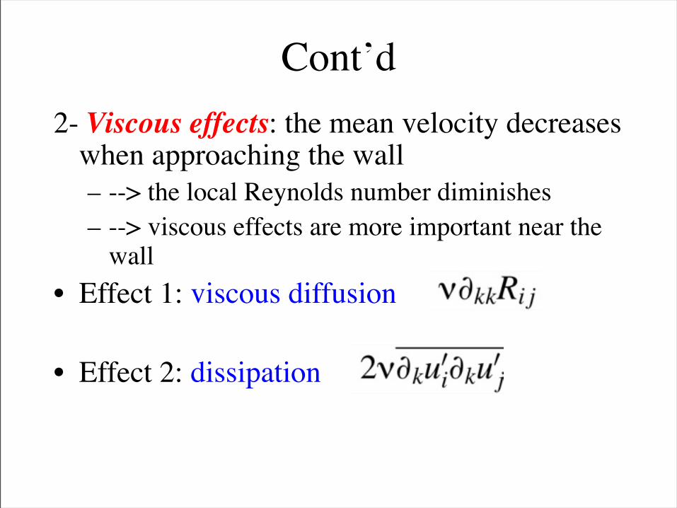
Cont’d2- Viscous effects: the mean velocity decreases

when approaching the wall– --> the local Reynolds number diminishes– --> viscous effects are more important near the

wall• Effect 1: viscous diffusion

• Effect 2: dissipation

Cont’d3- Effects due to the impermeability assumption

– Kinematic « splash » effect: structures impinging the wall induce a redistribution of TKE from wall-normal toward tangential velocity components

• --> damping of the wall-normal Reynolds stress• --> increase of the 2 other diagonal stresses• --> increase of anisotropy

Note: also present in shear-free boundary layer (e.g. boundary layer developing above a moving belt)

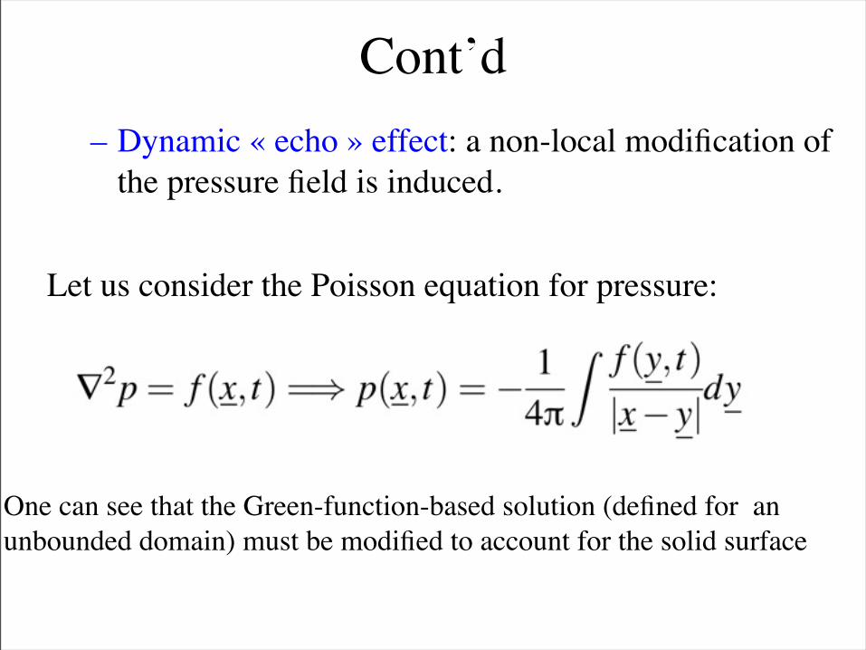
Cont’d– Dynamic « echo » effect: a non-local modification of

the pressure field is induced.

Let us consider the Poisson equation for pressure:

One can see that the Green-function-based solution (defined for an unbounded domain) must be modified to account for the solid surface

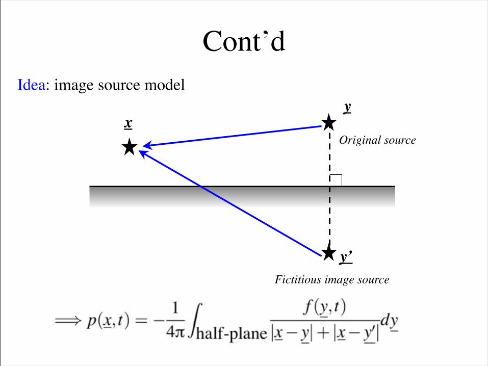
Cont’dIdea: image source model

xy

y’

Original source

Fictitious image source

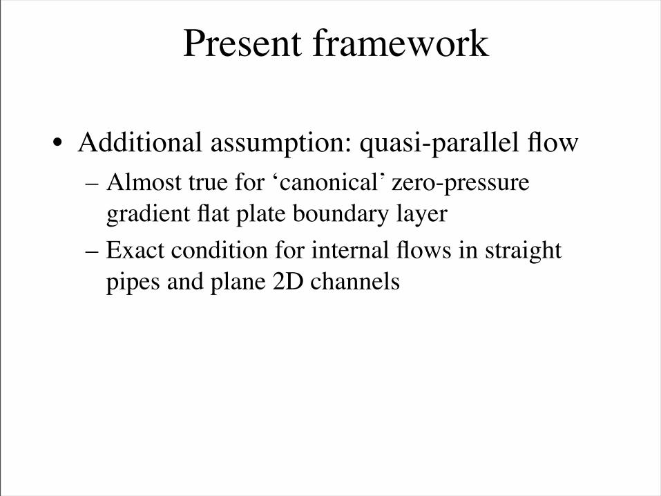
• Additional assumption: quasi-parallel flow– Almost true for ‘canonical’ zero-pressure

gradient flat plate boundary layer– Exact condition for internal flows in straight

pipes and plane 2D channels

Present framework

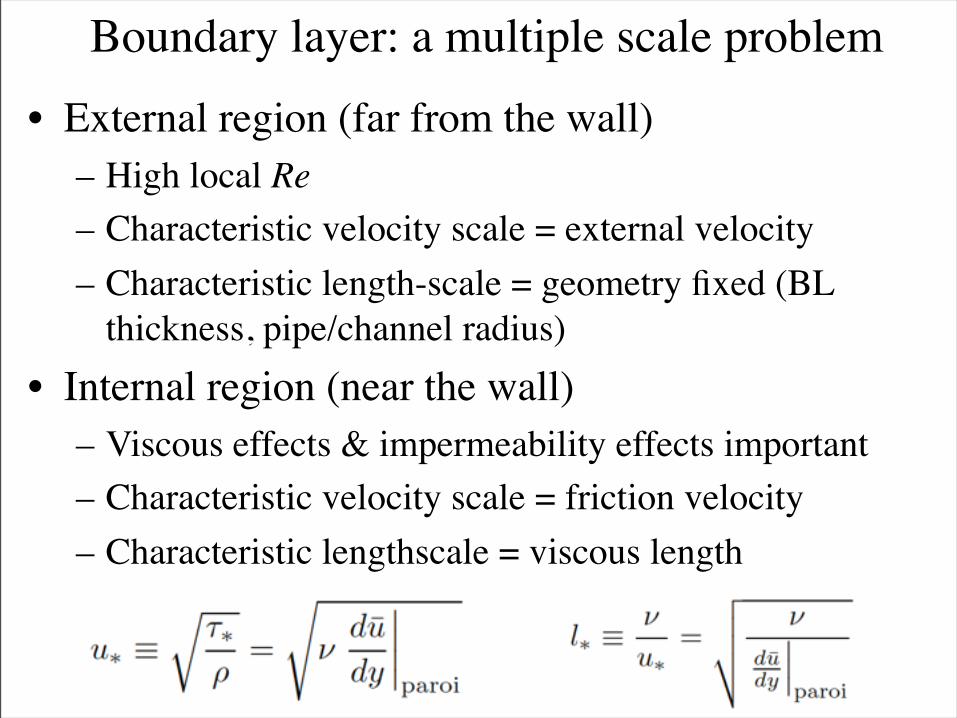
Boundary layer: a multiple scale problem• External region (far from the wall)

– High local Re– Characteristic velocity scale = external velocity– Characteristic length-scale = geometry fixed (BL

thickness, pipe/channel radius)• Internal region (near the wall)

– Viscous effects & impermeability effects important– Characteristic velocity scale = friction velocity– Characteristic lengthscale = viscous length

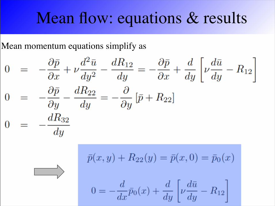
Mean flow: equations & resultsMean momentum equations simplify as

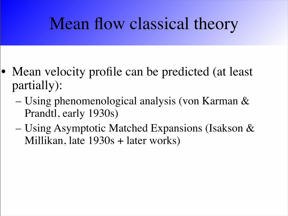
Mean flow classical theory

• Mean velocity profile can be predicted (at least partially):– Using phenomenological analysis (von Karman &

Prandtl, early 1930s) – Using Asymptotic Matched Expansions (Isakson &

Millikan, late 1930s + later works)

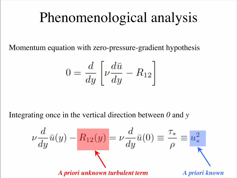
Phenomenological analysis

Momentum equation with zero-pressure-gradient hypothesis

Integrating once in the vertical direction between 0 and y

A priori unknown turbulent term A priori known

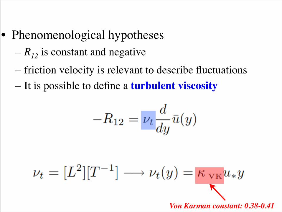
• Phenomenological hypotheses– R12 is constant and negative– friction velocity is relevant to describe fluctuations– It is possible to define a turbulent viscosity

Von Karman constant: 0.38-0.41

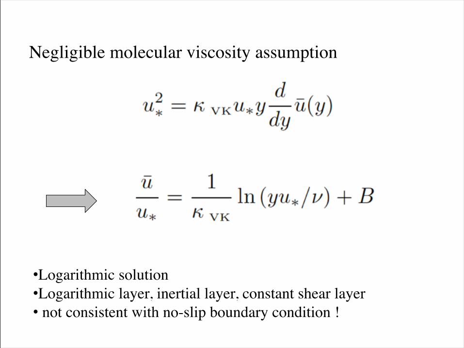
Negligible molecular viscosity assumption

•Logarithmic solution•Logarithmic layer, inertial layer, constant shear layer• not consistent with no-slip boundary condition !

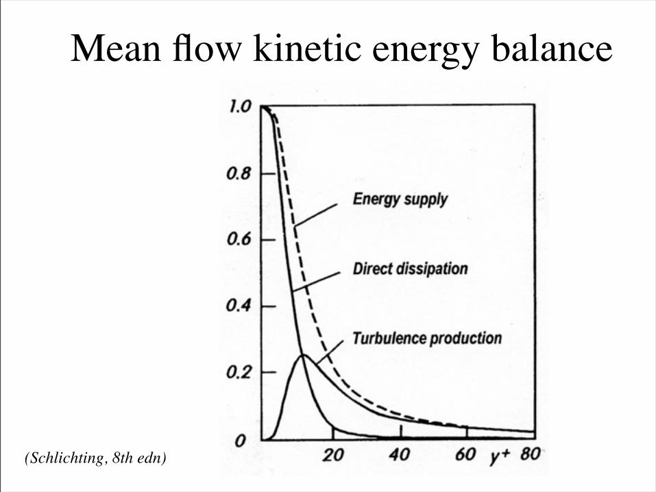
Mean flow kinetic energy balance

(Schlichting, 8th edn)

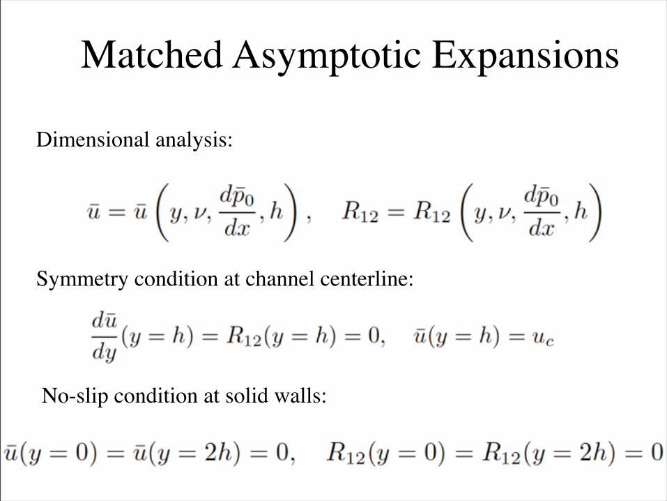
Matched Asymptotic Expansions

Dimensional analysis:

Symmetry condition at channel centerline:

No-slip condition at solid walls:

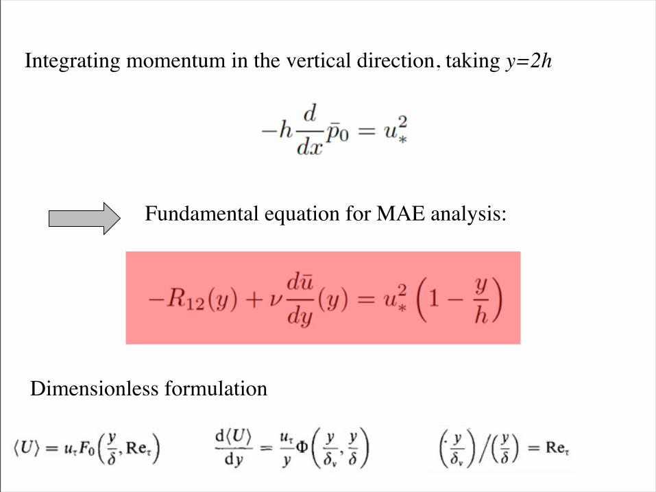
Integrating momentum in the vertical direction, taking y=2h

Fundamental equation for MAE analysis:

Dimensionless formulation

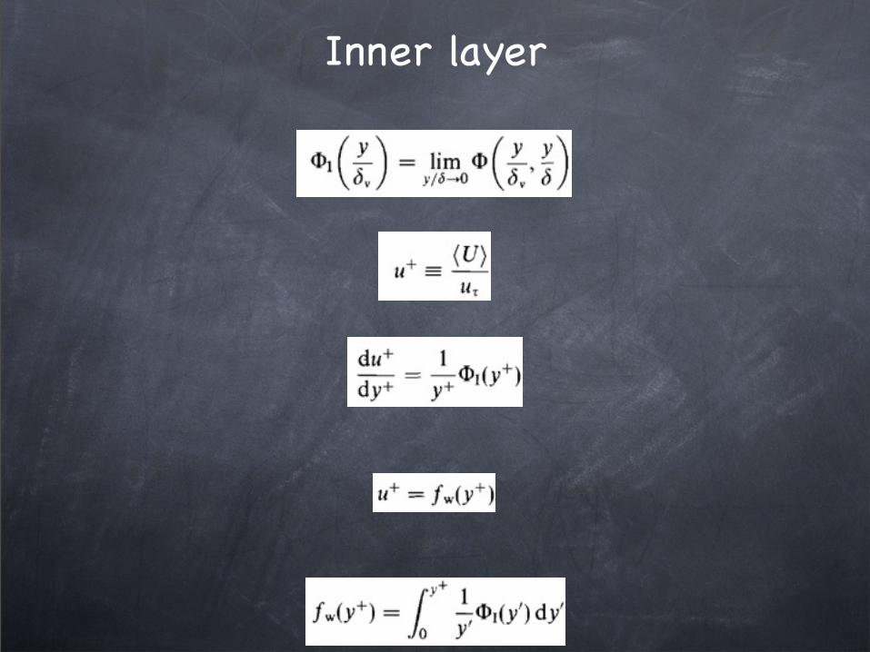
Inner layer

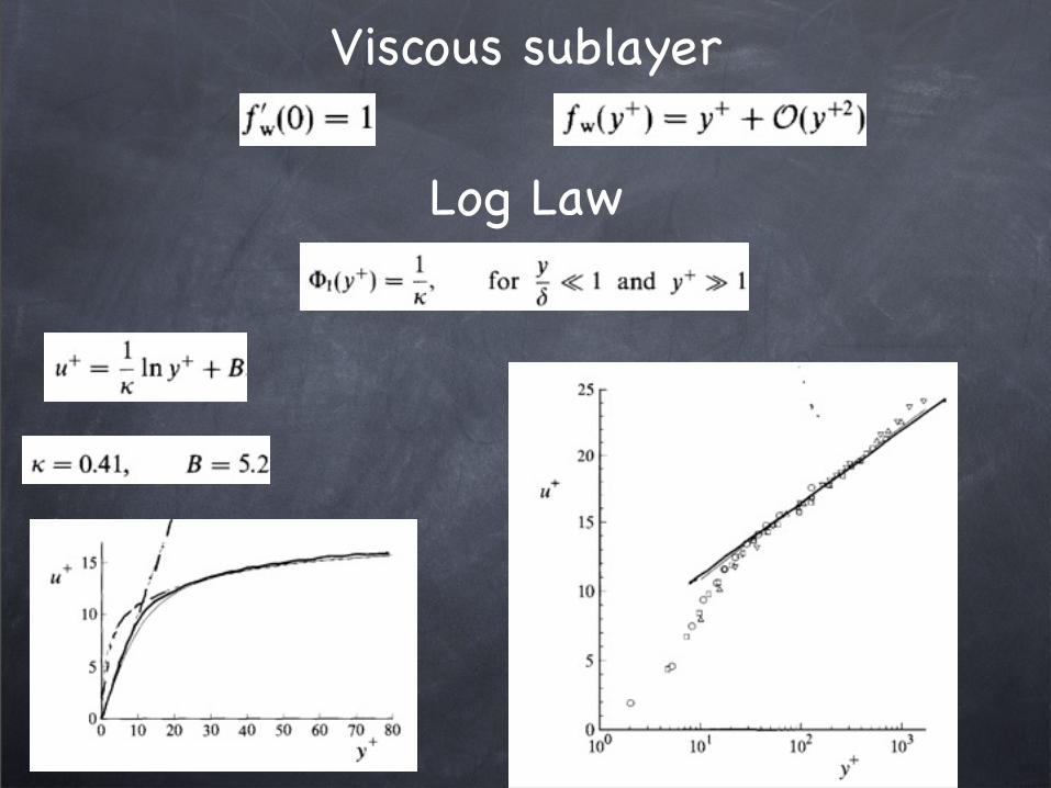
Viscous sublayer

Log Law

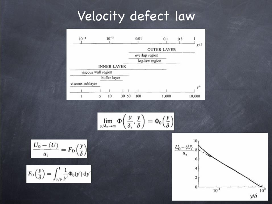
Velocity defect law

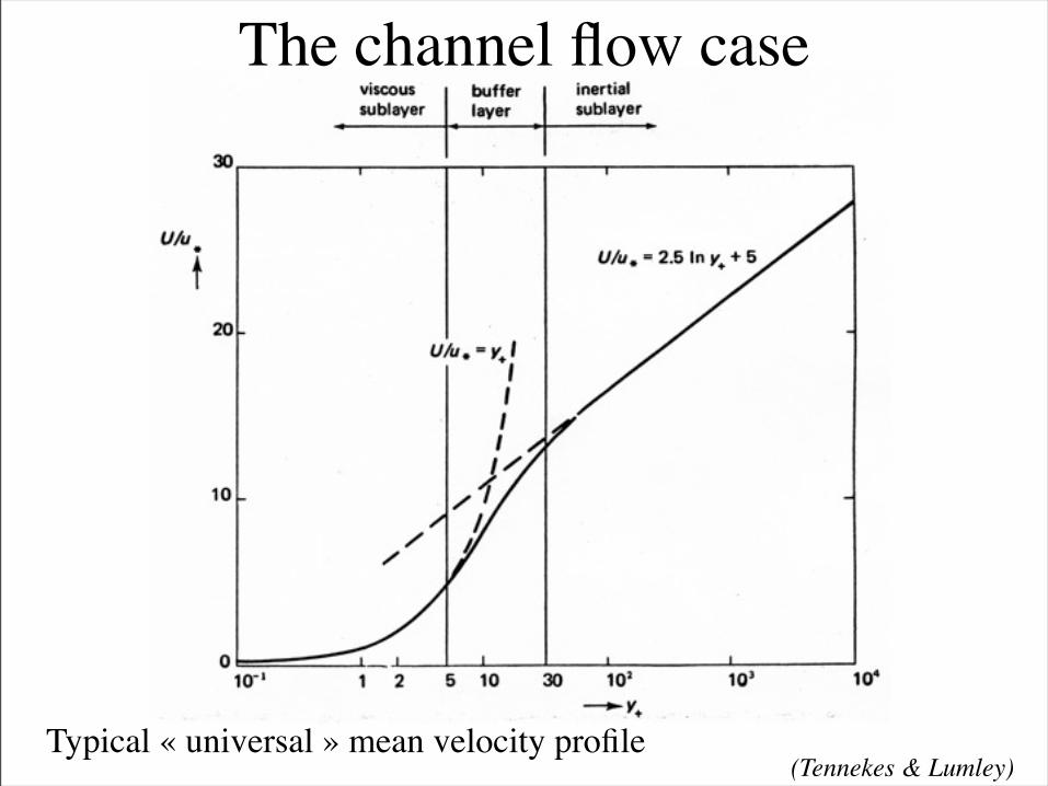
The channel flow case

Typical « universal » mean velocity profile(Tennekes & Lumley)

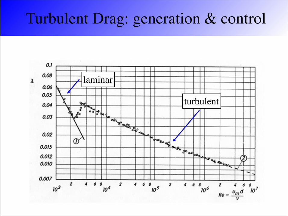
Turbulent Drag: generation & control

laminar

turbulent

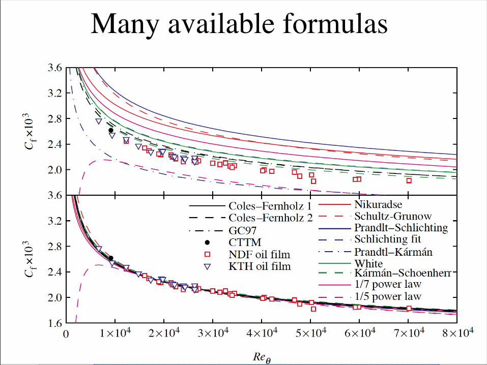
Many available formulas

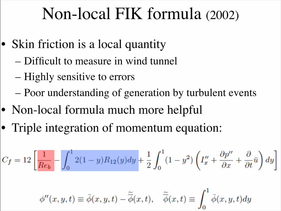
Non-local FIK formula (2002)

• Skin friction is a local quantity– Difficult to measure in wind tunnel– Highly sensitive to errors– Poor understanding of generation by turbulent events

• Non-local formula much more helpful• Triple integration of momentum equation:

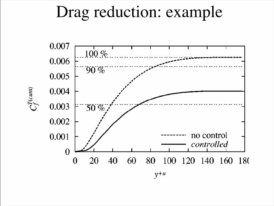
Drag reduction: example

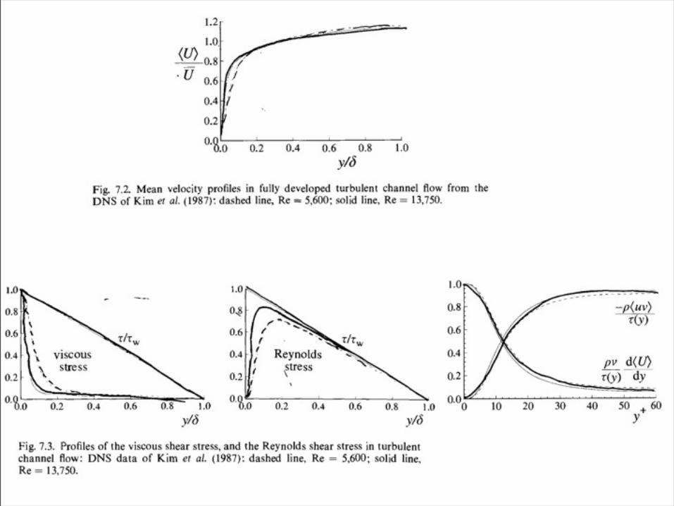
Reynolds stresses & TKE balance

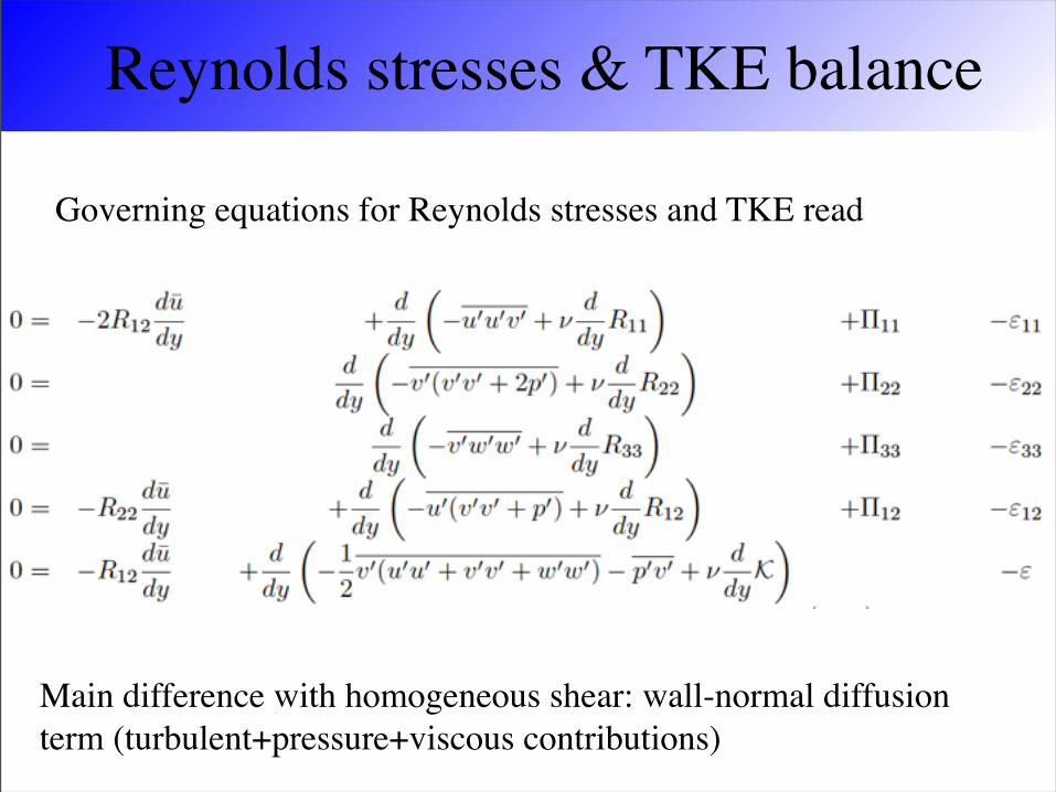
Governing equations for Reynolds stresses and TKE read

Main difference with homogeneous shear: wall-normal diffusion term (turbulent+pressure+viscous contributions)

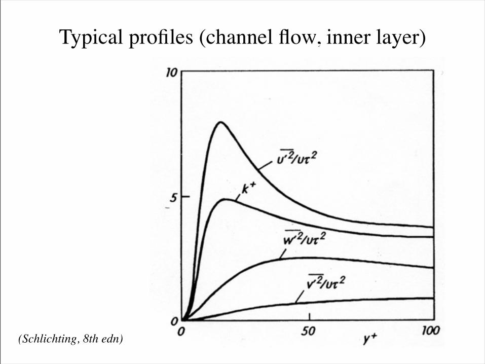
Typical profiles (channel flow, inner layer)

(Schlichting, 8th edn)

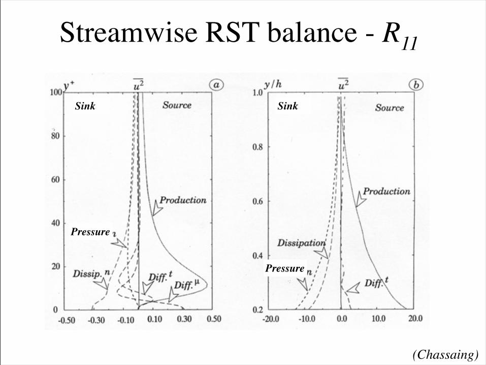
Streamwise RST balance - R11

Sink Sink

Pressure

Pressure

(Chassaing)

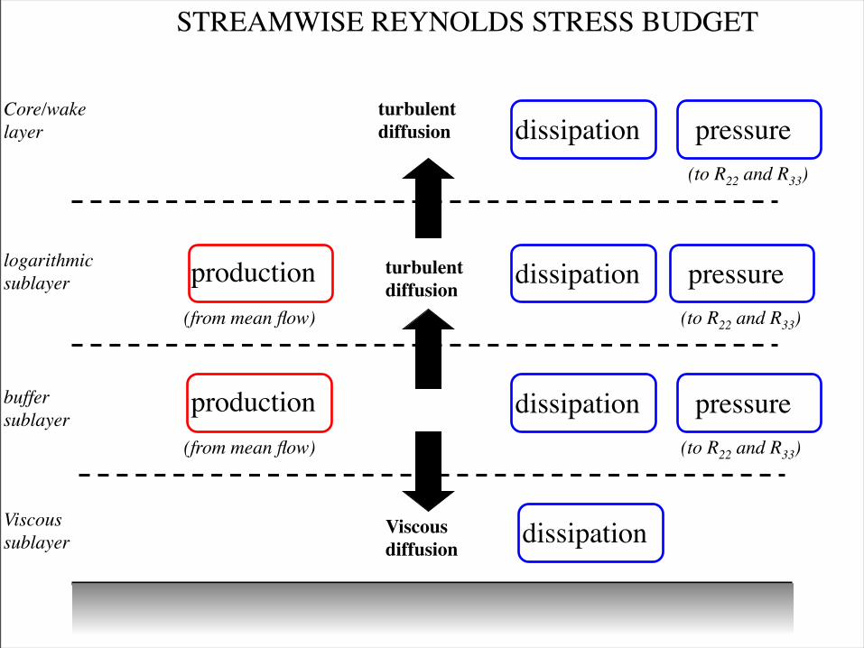
Viscoussublayer

buffersublayer

logarithmicsublayer

Core/wakelayer

dissipation

dissipation

dissipation

dissipation

production

production

Viscousdiffusion

turbulentdiffusion

turbulentdiffusion

pressure

pressure

pressure

STREAMWISE REYNOLDS STRESS BUDGET

(from mean flow)

(from mean flow) (to R22 and R33)

(to R22 and R33)

(to R22 and R33)

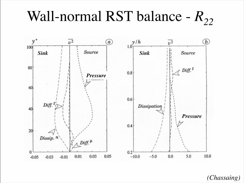
Wall-normal RST balance - R22

Sink Sink

Pressure

Pressure

(Chassaing)

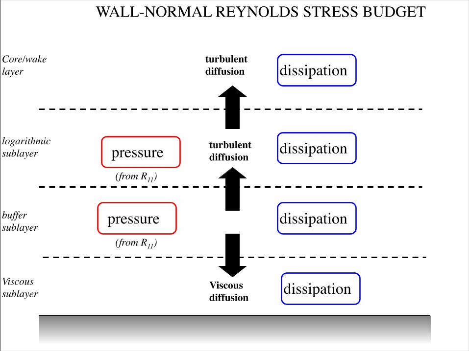
Viscoussublayer

buffersublayer

logarithmicsublayer

Core/wakelayer

dissipation

dissipation

dissipation

dissipation

Viscousdiffusion

turbulentdiffusion

turbulentdiffusion

pressure

WALL-NORMAL REYNOLDS STRESS BUDGET

pressure

(from R11)

(from R11)

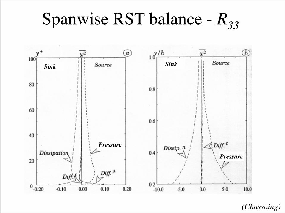
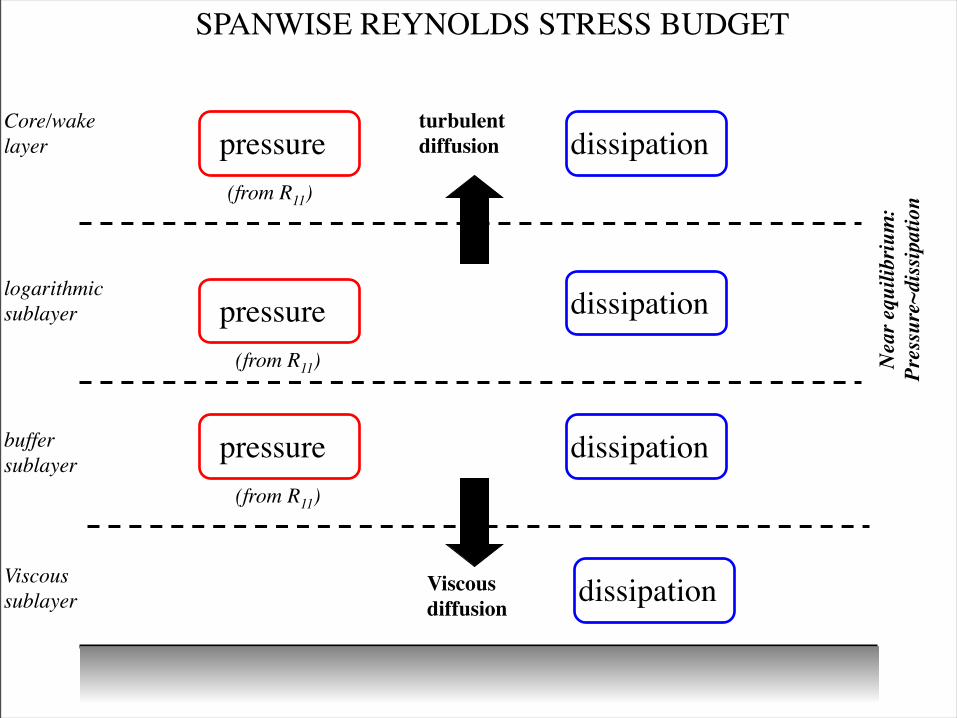
Spanwise RST balance - R33

Sink Sink

Pressure

Pressure

(Chassaing)

Viscoussublayer

buffersublayer

logarithmicsublayer

Core/wakelayer

dissipation

dissipation

dissipation

dissipation

Viscousdiffusion

turbulentdiffusion

pressure

SPANWISE REYNOLDS STRESS BUDGET

pressure

(from R11)

(from R11)

pressure(from R11)

Nea

r equ

ilibr

ium

:Pr

essu

re~d

issip

atio

n

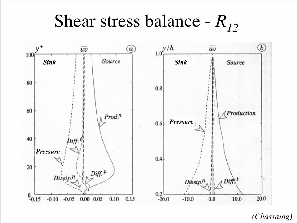
Shear stress balance - R12

Sink Sink

Pressure

Pressure

(Chassaing)

Viscoussublayer

buffersublayer

logarithmicsublayer

Core/wakelayer

dissipationViscousdiffusion

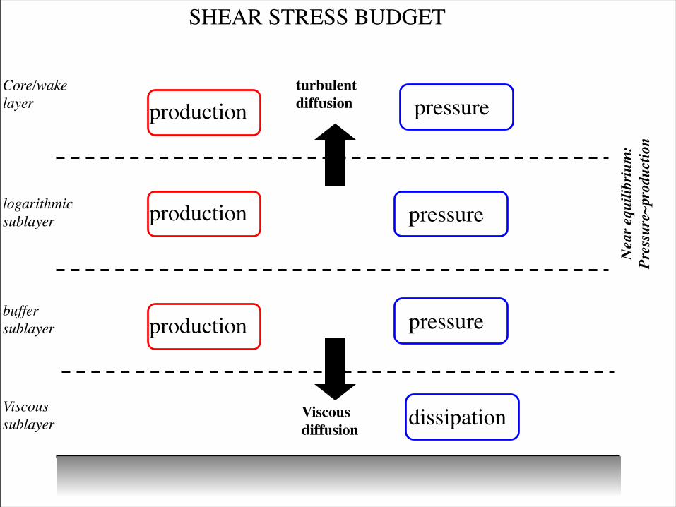
SHEAR STRESS BUDGET

turbulentdiffusion

production

production

production

pressure

pressure

pressure

Nea

r equ

ilibr

ium

:Pr

essu

re~p

rodu

ctio

n

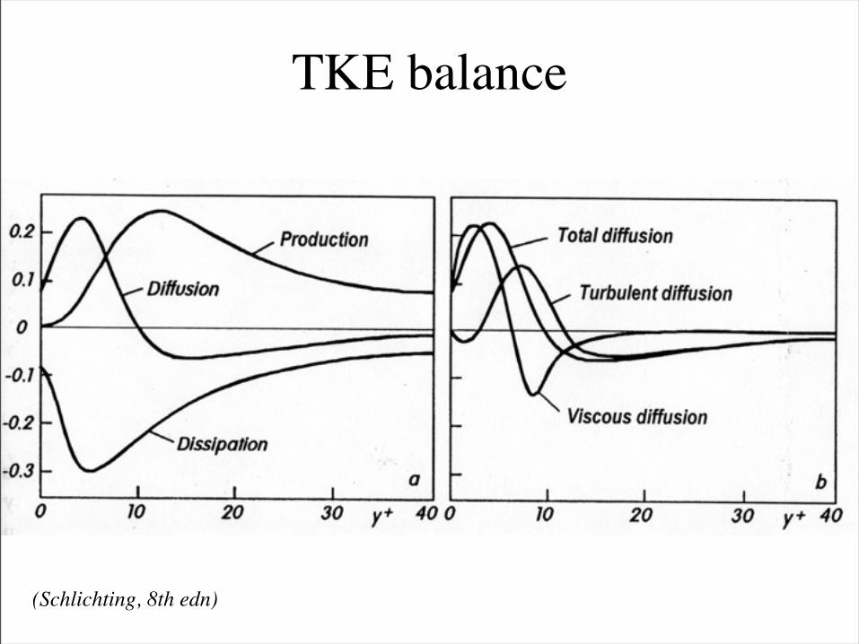
TKE balance

(Schlichting, 8th edn)

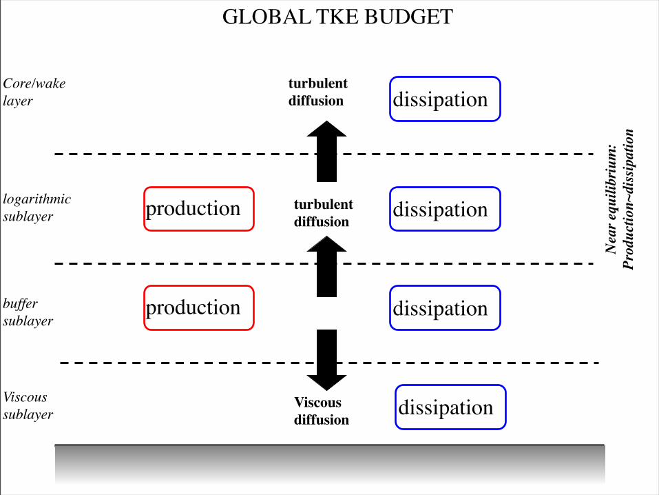
Viscoussublayer

buffersublayer

logarithmicsublayer

Core/wakelayer

dissipation

dissipation

dissipation

dissipation

production

production

Viscousdiffusion

turbulentdiffusion

turbulentdiffusion

Nea

r equ

ilibr

ium

:Pr

oduc

tion~

diss

ipat

ion

GLOBAL TKE BUDGET

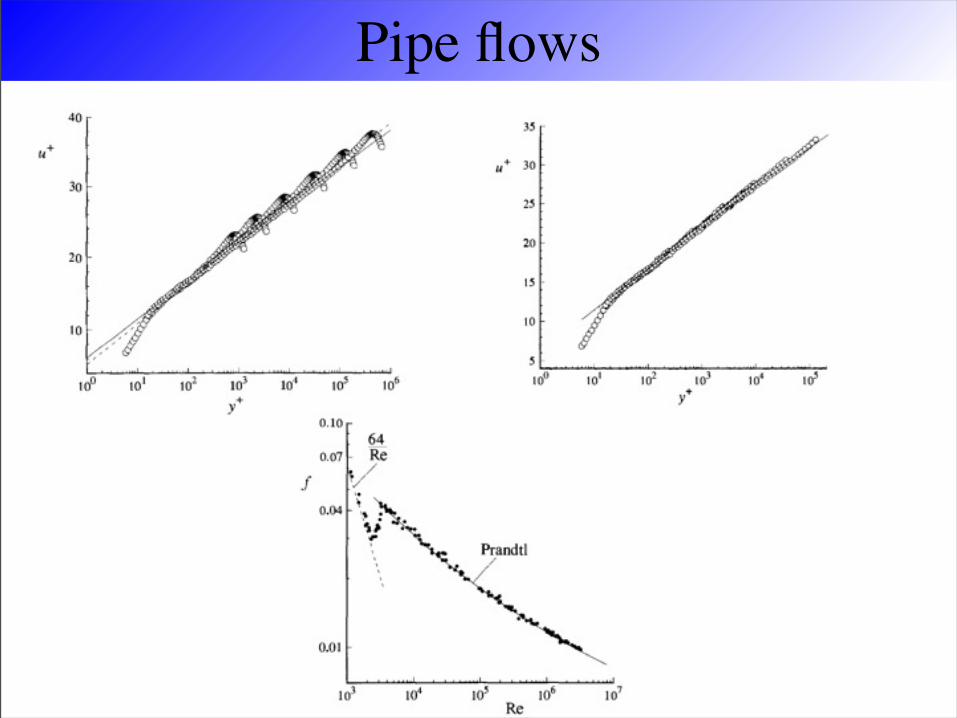
Pipe flows

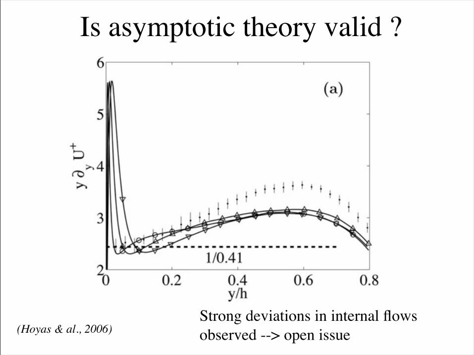
Is asymptotic theory valid ?

(Hoyas & al., 2006)Strong deviations in internal flows observed --> open issue

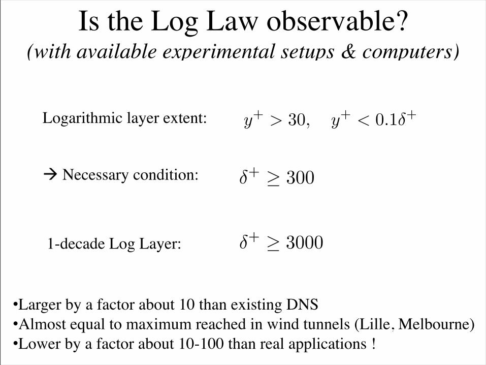
Is the Log Law observable?(with available experimental setups & computers)

Logarithmic layer extent: y+ > 30, y+ < 0.1δ+

Necessary condition: δ+ ≥ 300

1-decade Log Layer: δ+ ≥ 3000

•Larger by a factor about 10 than existing DNS•Almost equal to maximum reached in wind tunnels (Lille, Melbourne)•Lower by a factor about 10-100 than real applications !

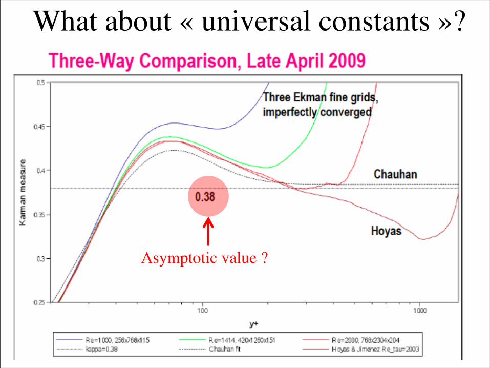
What about « universal constants »?

Asymptotic value ?

Roughness effects

• Previous results hold for « ideally smooth » surfaces

• Real materials are not perfect– --> a new lengthscale is involved to describe

rugous walls: – --> how are previous results modified ?

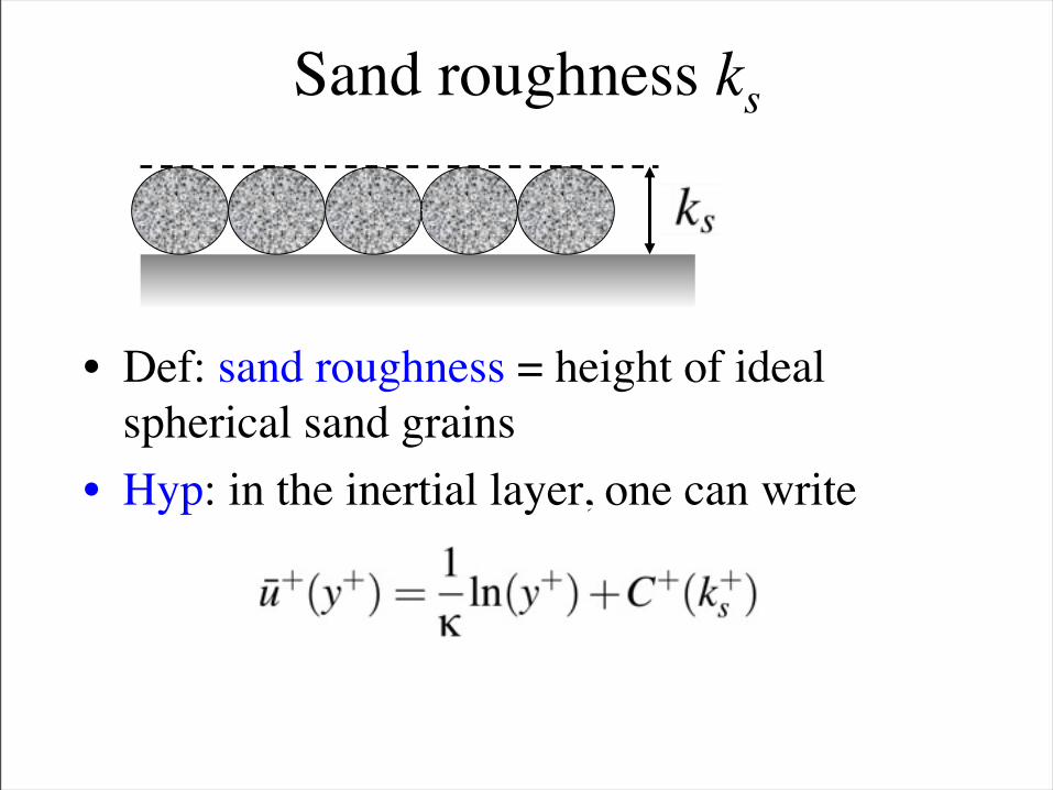
Sand roughness ks

• Def: sand roughness = height of ideal spherical sand grains

• Hyp: in the inertial layer, one can write

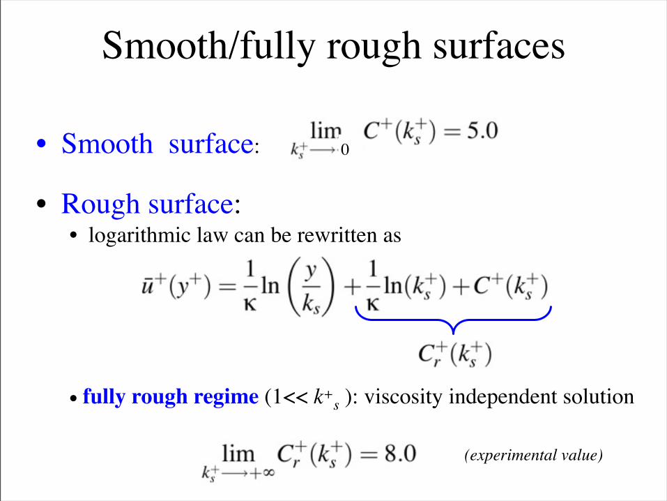
Smooth/fully rough surfaces

• Smooth surface:

• Rough surface:• logarithmic law can be rewritten as

• fully rough regime (1<< k+s ): viscosity independent solution

(experimental value)

0

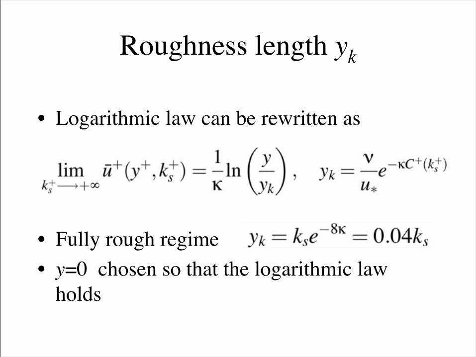
Roughness length yk

• Logarithmic law can be rewritten as

• Fully rough regime• y=0 chosen so that the logarithmic law

holds

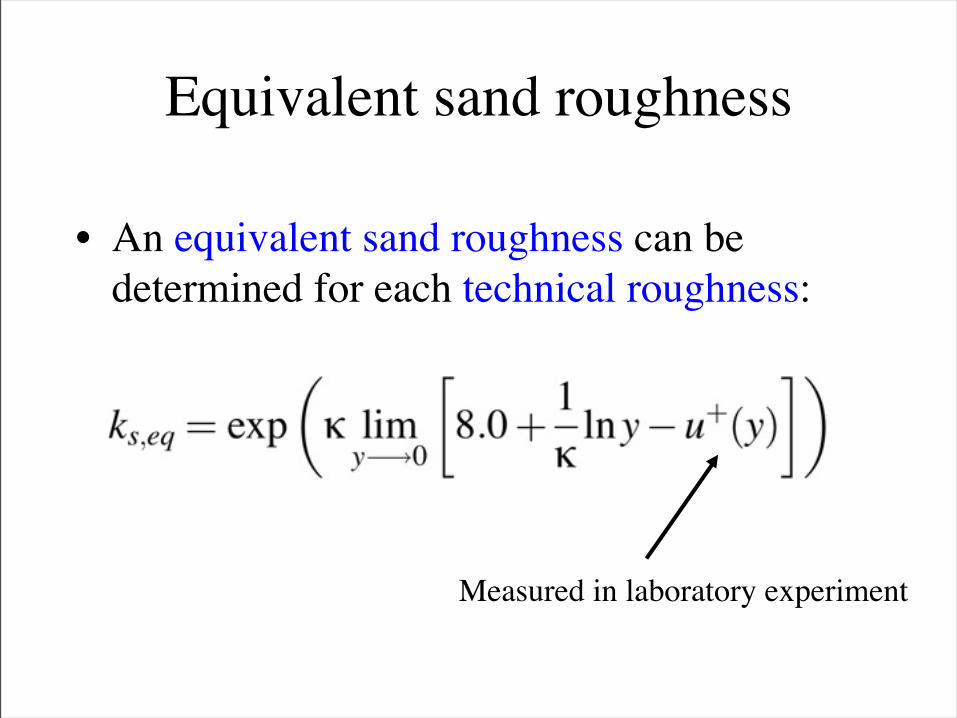
Equivalent sand roughness

• An equivalent sand roughness can be determined for each technical roughness:

Measured in laboratory experiment

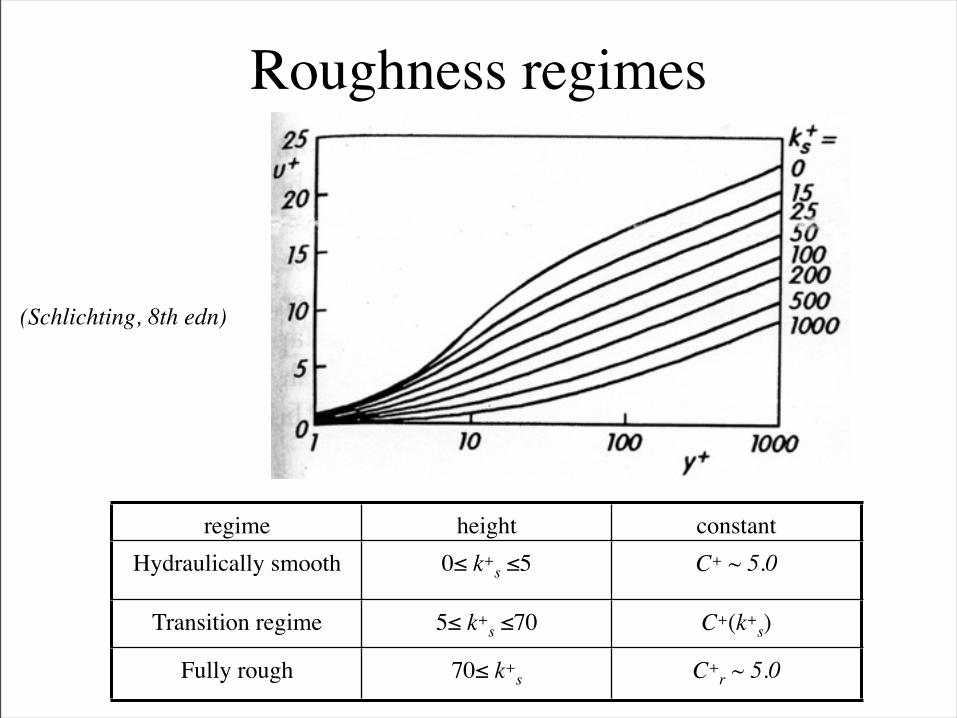
Roughness regimes

(Schlichting, 8th edn)

regime height constantHydraulically smooth 0≤ k+

s ≤5 C+ ~ 5.0

Transition regime 5≤ k+s ≤70 C+(k+

s)

Fully rough 70≤ k+s C+

r ~ 5.0

Coherent structures & turbulence dynamics

• The dynamics is associated with a very complex instantaneous flow organization

• Several types of flow structures are observed• Each layer exhibits different coherent events• Identification of the exact role of each

structure is still an open controversial issue

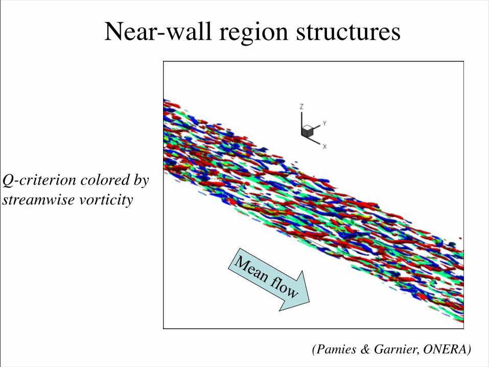
Near-wall region structures

Mean flow

Q-criterion colored by streamwise vorticity

(Pamies & Garnier, ONERA)

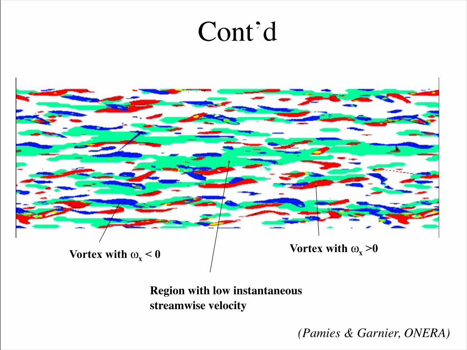
Cont’d

Vortex with ωx >0Vortex with ωx < 0

(Pamies & Garnier, ONERA)

Region with low instantaneous streamwise velocity

What is observed in viscous/buffer layers:

• Low/high-speed Streamwise velocity streaks : sinuous arrays of alternating streamwise jets superimposed on the mean shear (Kim & al., 1971) – Average spanwise wavelength z+=50-100 (Smith & al.,

1983)– Average streamwise length x+=1000– Wall shear is higher than the average at locations where

the jets point forward (resp. backward) for high speed (resp. low speed) streaks

Cont’d• Quasi-streamwise vortices

– Slightly tilted from the wall– Stay in the near-wall region only for x+=200

(Jeong & al., 1997)– Several vortices are associated with each streak, with

longitudinal spacing x+=400– Some of them are connected to legs of hairpin vortices

in the log layer, but most merge in uncoherent vorticity away from the wall

– Are advected at speed c+=10

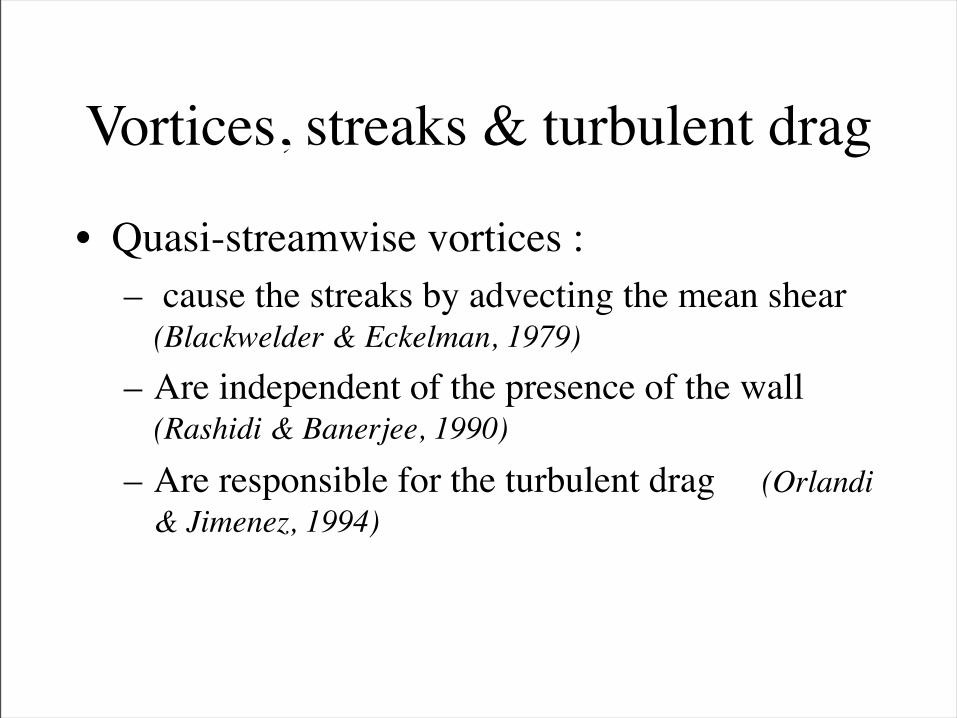
Vortices, streaks & turbulent drag

• Quasi-streamwise vortices :– cause the streaks by advecting the mean shear

(Blackwelder & Eckelman, 1979)– Are independent of the presence of the wall

(Rashidi & Banerjee, 1990)– Are responsible for the turbulent drag (Orlandi

& Jimenez, 1994)

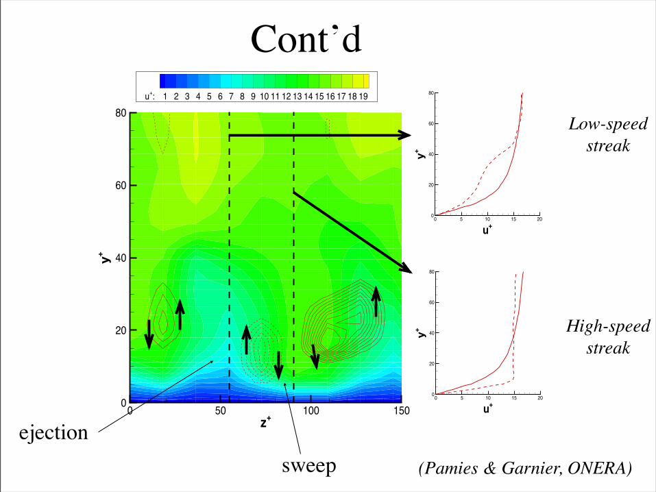
Cont’d

z+

y+

0 50 100 1500

20

40

60

80

u+: 1 2 3 4 5 6 7 8 9 10 11 12 13 14 15 16 17 18 19

u+

y+

0 5 10 15 200

20

40

60

80

u+

y+

0 5 10 15 200

20

40

60

80

High-speedstreak

Low-speedstreak

(Pamies & Garnier, ONERA)

ejectionsweep

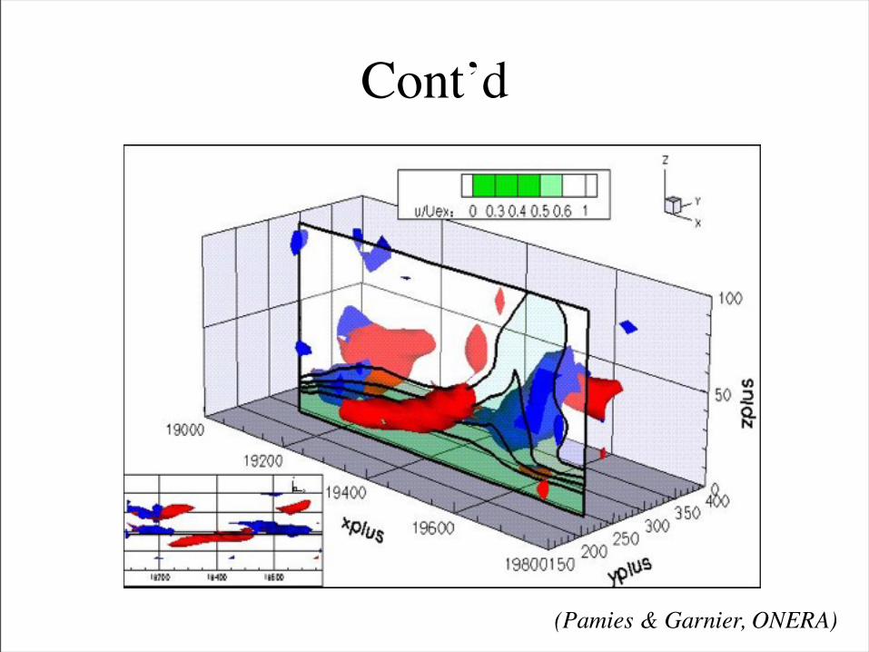
Cont’d

(Pamies & Garnier, ONERA)

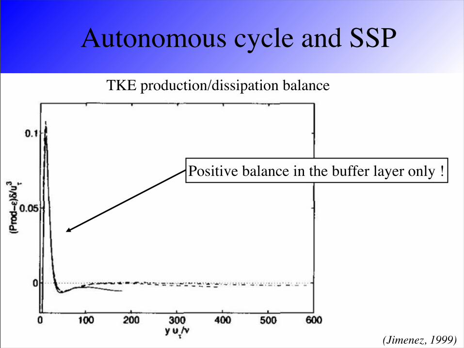
Autonomous cycle and SSP

(Jimenez, 1999)

TKE production/dissipation balance

Positive balance in the buffer layer only !

Cont’d

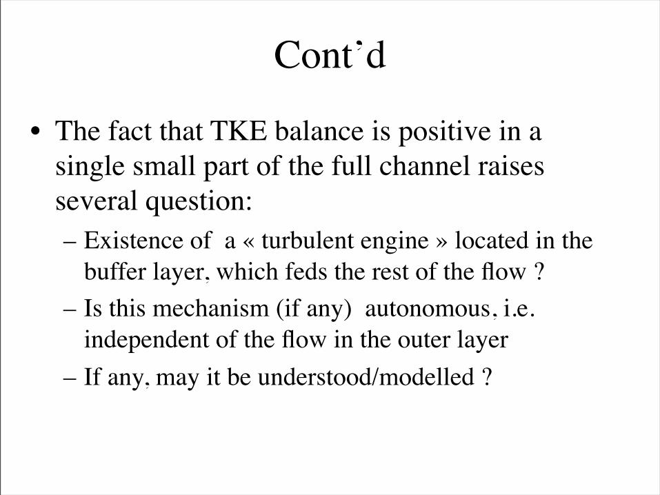
• The fact that TKE balance is positive in a single small part of the full channel raises several question:– Existence of a « turbulent engine » located in the

buffer layer, which feds the rest of the flow ?– Is this mechanism (if any) autonomous, i.e.

independent of the flow in the outer layer– If any, may it be understood/modelled ?

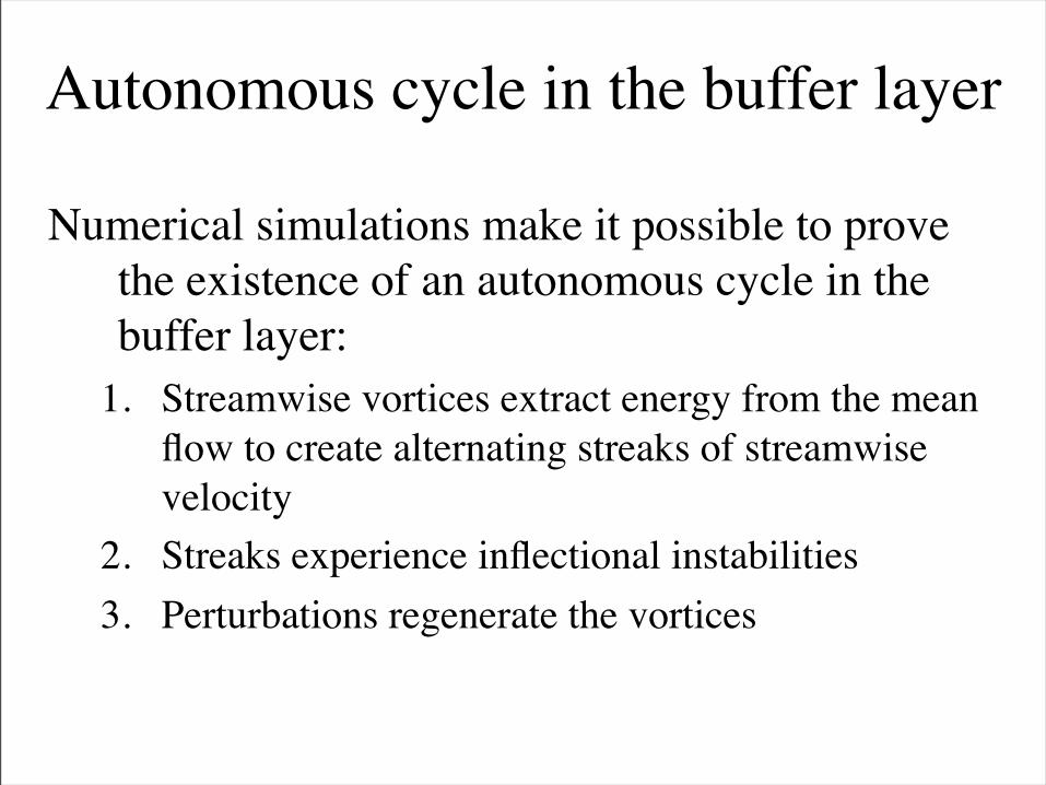
Autonomous cycle in the buffer layer

Numerical simulations make it possible to prove the existence of an autonomous cycle in the buffer layer:

1. Streamwise vortices extract energy from the mean flow to create alternating streaks of streamwise velocity

2. Streaks experience inflectional instabilities3. Perturbations regenerate the vortices

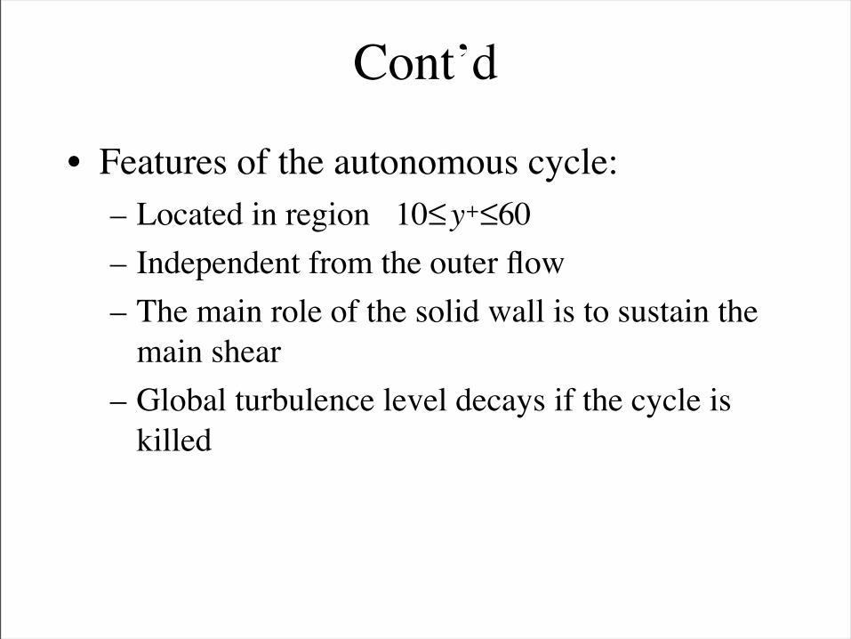
Cont’d

• Features of the autonomous cycle:– Located in region 10≤ y+≤60– Independent from the outer flow– The main role of the solid wall is to sustain the

main shear– Global turbulence level decays if the cycle is

killed

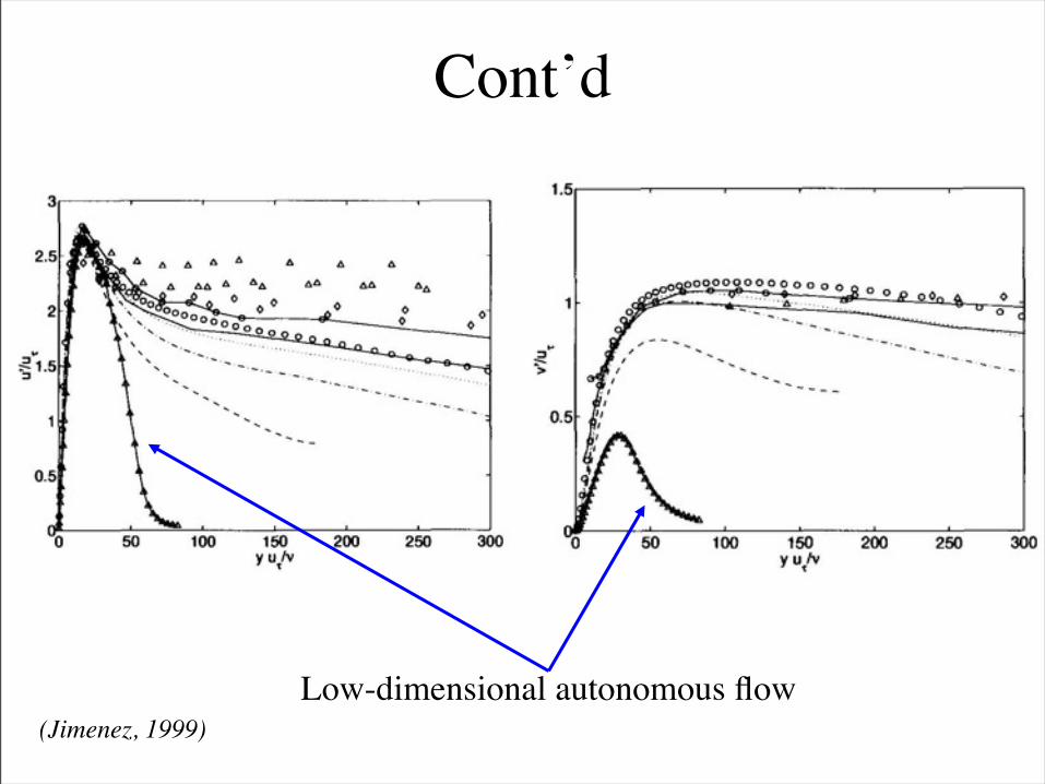
Cont’d

(Jimenez, 1999)Low-dimensional autonomous flow

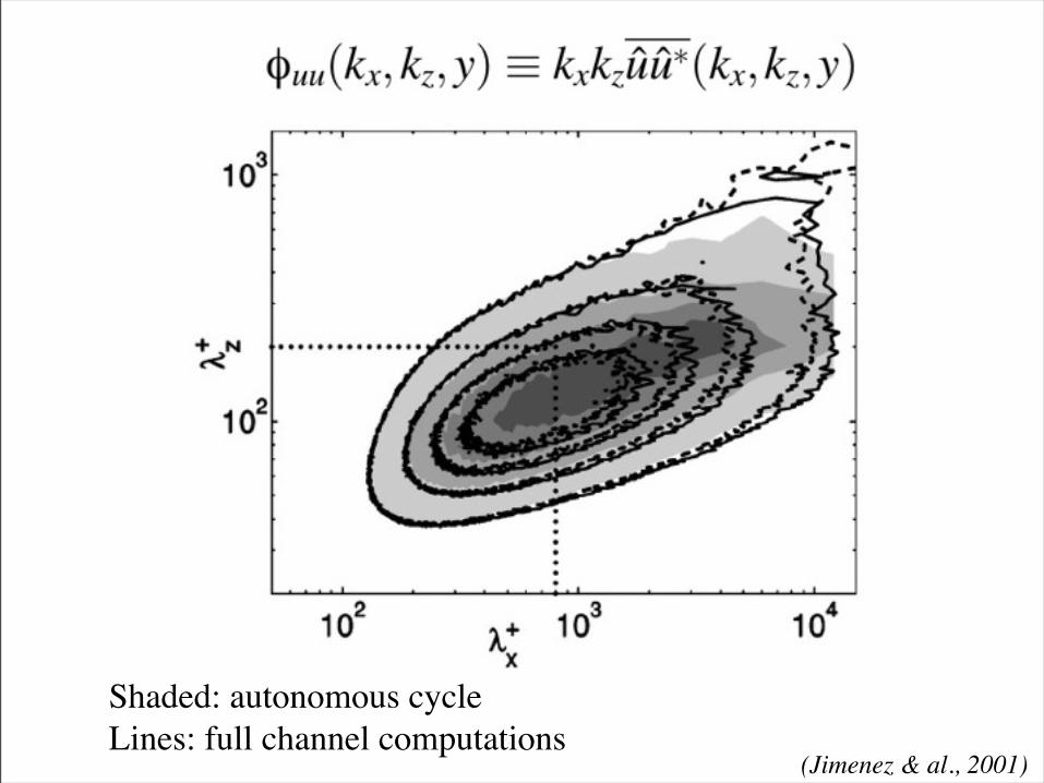
(Jimenez & al., 2001)

Shaded: autonomous cycleLines: full channel computations

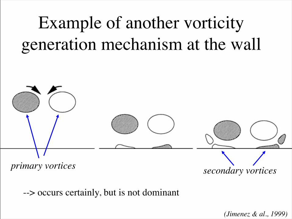
Example of another vorticity generation mechanism at the wall

(Jimenez & al., 1999)

primary vortices secondary vortices

--> occurs certainly, but is not dominant

Minimal wall flow (Jimenez & Moin, 1991)

• Concept: what is the size of the smallest box in which the cycle is sustained ?

• Numerical experiments lead to λx+ ≈ λz

+ ≈150• Typical pattern: one wavy low-speed streak

flanked by two quasi-streamwise vortices

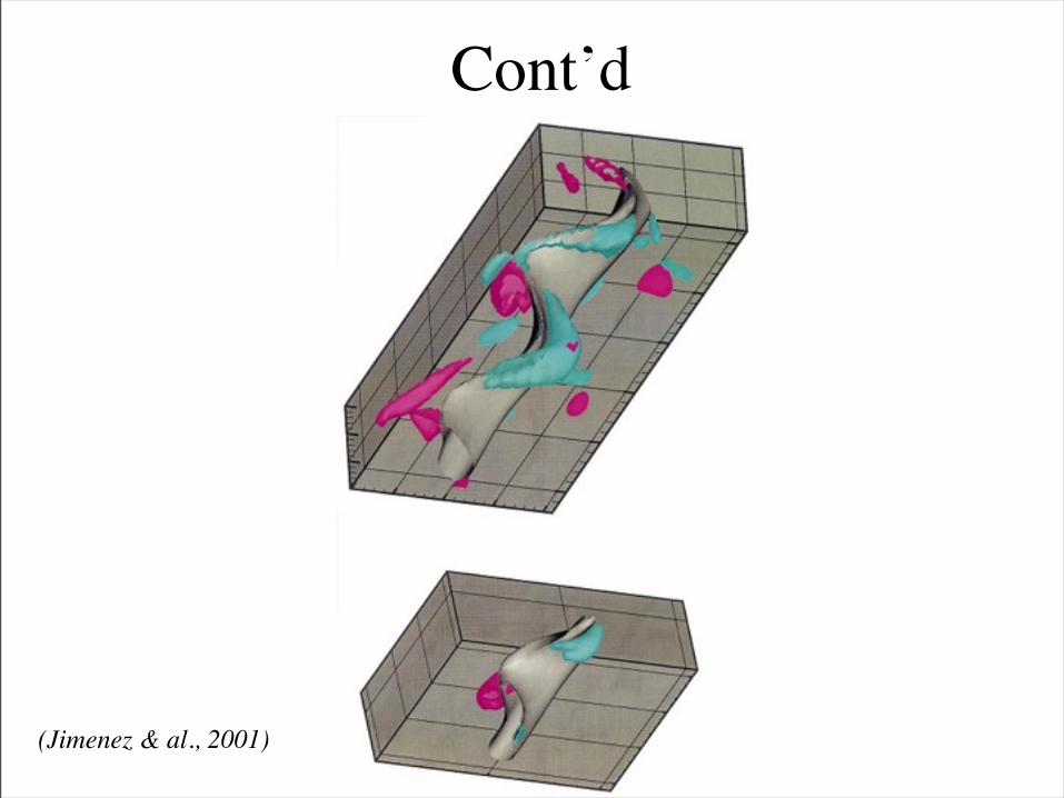
Cont’d

(Jimenez & al., 2001)

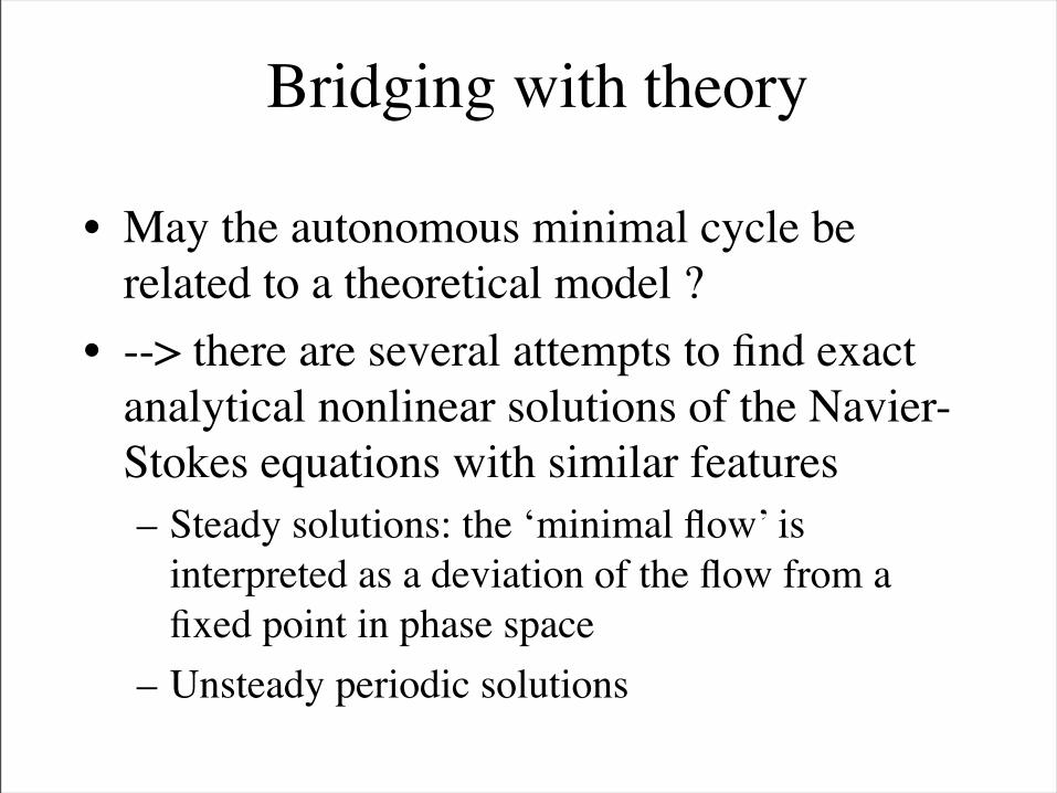
Bridging with theory

• May the autonomous minimal cycle be related to a theoretical model ?

• --> there are several attempts to find exact analytical nonlinear solutions of the Navier-Stokes equations with similar features– Steady solutions: the ‘minimal flow’ is

interpreted as a deviation of the flow from a fixed point in phase space

– Unsteady periodic solutions

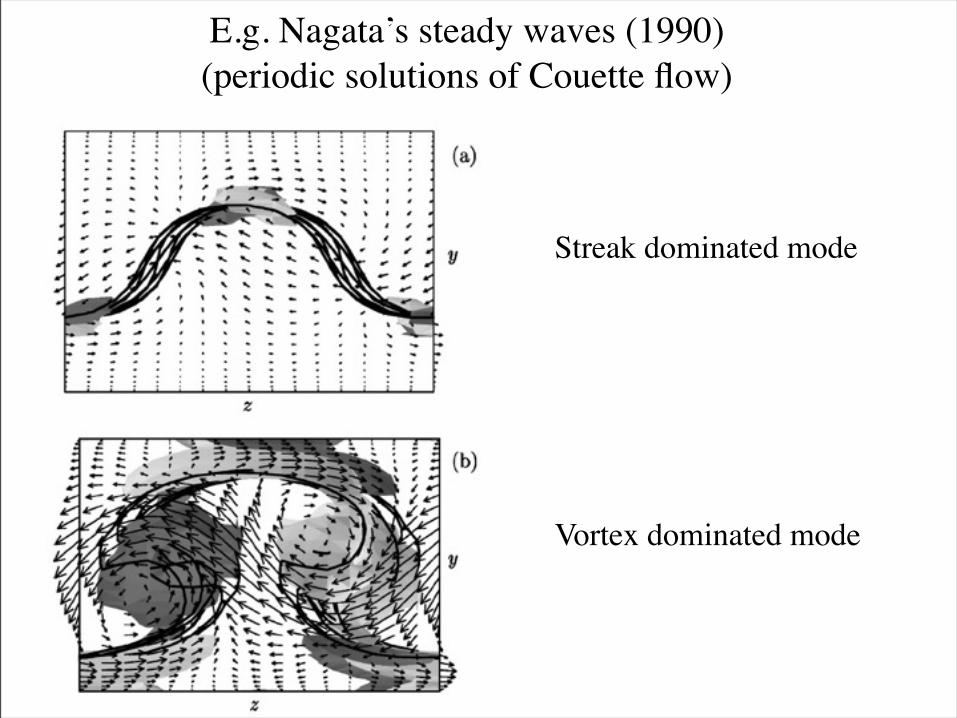
E.g. Nagata’s steady waves (1990)(periodic solutions of Couette flow)

Streak dominated mode

Vortex dominated mode