Tuffy: Scaling up Statistical Inference in Markov LogicNetworks using an RDBMS

Feng Niu Christopher Ré AnHai Doan Jude ShavlikUniversity of Wisconsin-Madison

{leonn,chrisre,anhai,shavlik}@cs.wisc.edu

ABSTRACTOver the past few years, Markov Logic Networks (MLNs)have emerged as a powerful AI framework that combinesstatistical and logical reasoning. It has been applied to awide range of data management problems, such as informa-tion extraction, ontology matching, and text mining, andhas become a core technology underlying several major AIprojects. Because of its growing popularity, MLNs are partof several research programs around the world. None ofthese implementations, however, scale to large MLN datasets. This lack of scalability is now a key bottleneck thatprevents the widespread application of MLNs to real-worlddata management problems.

In this paper we consider how to leverage RDBMSes todevelop a solution to this problem. We consider Alchemy,the state-of-the-art MLN implementation currently in wideuse. We first develop bTuffy, a system that implementsAlchemy in an RDBMS. We show that bTuffy alreadyscales to much larger datasets than Alchemy, but suffersfrom a sequential processing problem (inherent in Alchemy).We then propose cTuffy that makes better use of the RDBMS’sset-at-a-time processing ability. We show that this pro-duces dramatic benefits: on all four benchmarks cTuffydominates both Alchemy and bTuffy. Moreover, on thecomplex entity resolution benchmark cTuffy finds a solu-tion in minutes, while Alchemy spends hours unsuccessfully.We summarize the lessons we learnt, on how we can designAI algorithms to take advantage of RDBMSes, and extendRDBMSes to work better for AI algorithms.

1. INTRODUCTIONOver the past few years, Markov Logic Networks (MLNs)

have emerged as a powerful and popular framework thatcombines logical and probabilistic reasoning. It has beensuccessfully applied to a wide variety of data managementproblems, including information extraction, entity resolu-tion, and text mining. In fact, it has become a core tech-nology underlying several large projects, such as the DARPA

Permission to copy without fee all or part of this material is granted providedthat the copies are not made or distributed for direct commercial advantage,the VLDB copyright notice and the title of the publication and its date appear,and notice is given that copying is by permission of the Very Large DataBase Endowment. To copy otherwise, or to republish, to post on serversor to redistribute to lists, requires a fee and/or special permission from thepublisher, ACM.VLDB ‘10, September 13-17, 2010, SingaporeCopyright 2010 VLDB Endowment, ACM 000-0-00000-000-0/00/00.

CALO and Machine Reading five-year programs. The frame-work has also been implemented at many academic and in-dustrial places, including Stanford, SRI, Washington, Wis-consin, and the University of Massachusetts at Amherst.

Unfortunately, none of the current MLN implementationsscales beyond relatively small data sets (and even on many ofthese, they routinely take hours to run). The first obviousreason is that these are in-memory implementations. Assuch, they thrash badly when generating and manipulatinglarge intermediate data structures that overflow the mainmemory, which they very often do.

Consequently, there is an emerging effort across severalresearch groups to try to scale up MLNs. In this paper, weexplore the first obvious candidate, an RDBMS, to managethe memory overflow problem. In particular, DARPA, theresearch arm of the US Department of Defense, is currentlyrunning a large five-year program called “Machine Reading”.The goal is to build software that can “read” the Web, i.e.,extract and integrate structured data (e.g., entities, rela-tionships) from Web data, then use this structured data toanswer user queries. Within this program, the SRI team,a large research group spanning six universities and two in-dustrial labs (and across the AI and database communities),is considering how to apply MLNs to the machine readingproblem. To do so, it is critical that MLNs scale to largedata sets, and we have been put in charge of investigatingthis problem, partly because we are also interested in beingable to run MLNs to extract and integrate data within ourown Cimple/DBLife project.

This paper describes the result of our current investiga-tion. We seek to answer the following questions: Can anRDBMS help scale up MLNs? If yes, by how much, andwhat are the key reasons (beside the ability to manage datathat is larger than the main memory)? Given these rea-sons, in general how can we design AI algorithms to takeadvantage of RDBMSes? And how can we extend RDBM-Ses to work better for AI algorithms? As ever more pow-erful AI reasoning frameworks are being developed, answersto the above questions can help scale not just MLNs, butthose frameworks as well. Further, over the past decadethe database community has made a considerable effort toextend RDBMSes to deal with imprecise data, by pushingstatistical models into RDBMSes [1–4, 8, 13, 25, 33]. Ourwork on pushing MLNs into RDBMSes falls into, and canhelp advance, this emerging direction.

We began our investigation by designing bTuffy, a rela-tively straightforward implementation of MLNs in an RDBMS.We chose PostgreSQL because we want to eventually make

the code open source. Briefly, we store most of the data(original, intermediate, and final) in relational tables, andexecute most of the reasoning using SQL commands andqueries (§3). Reasoning with MLNs can be classified aseither learning or inference [21]. We focus on inference be-cause that tends to be performed multiple times online andso must be fast.

Next, we performed an extensive analysis of bTuffy. Asa comparison point, we select Alchemy, the currently mostpopular and state-of-the-art MLN implementation [5, 21].On a diverse set of tasks, we found that bTuffy significantlyoutperforms Alchemy. As expected, one of the reasons isthe ability to manage external data: whenever intermediatedata is larger than main memory, Alchemy thrashed badlywhereas bTuffy did not. But there is more. It turned outthat Alchemy performs many “relational operation”-likesteps (e.g., select, project, join) and that these operationsare often a bottleneck in MLN inference: on a classificationbenchmark over 96% of Alchemy’s execution time is spentperforming relational-like operations. To execute these op-erations, Alchemy uses fixed algorithms (e.g., always usingnested-loop join). In contrast, by exploiting the query op-timization strength of the RDBMS, bTuffy finds a goodway to execute these steps, thereby significantly speedingup MLN inference.

On the other hand, we found that bTuffy executed toomany SQL queries (as many as millions of queries on certaintasks), and this caused considerable overhead. This hap-pens because when Alchemy searches within a large spacefor the “world” with the highest probability (using Walk-SAT [10]), it performs an inherently sequential search. Itflips the value of a variable, does “book keeping” for a fairamount of time, determines based on that which variable toflip next, flips that variable, does book keeping again, andso on. Consequently, the natural solution of implementingeach step of flipping and book keeping with a SQL queryends up generating too many SQL queries, which must beexecuted sequentially.

To address this problem, we build on the MAXSAT lit-erature to design a new search algorithm where, concep-tually, multiple steps of flipping and book keeping can beexecuted in parallel, as a single group. We then implementeach group with a single SQL query, letting the RDBMS de-cide how best to execute the steps within the group. Assuch, this algorithm exploits the set-at-a-time-processingstrength of RDBMSes. Further, it runs drastically fewerSQL queries, thereby significantly reducing the overheadcompared to bTuffy. We refer to the RDBMS-based MLNsolution using this new search algorithm as cTuffy.

On a diverse set of MLN tasks obtained from the Web(including all applicable MLN tasks from the Alchemyrepository), we found that cTuffy dramatically outper-forms both bTuffy and Alchemy: on an entity resolu-tion task, cTuffy finds an optimal cost solution in 11 min-utes versus more than 7 hours for Alchemy or 2 hours forbTuffy.

To summarize, we make the following contributions:

• We developed a solution to push MLNs into RDBM-Ses, a problem of growing interest to both the databaseand AI communities. As far as we know, ours is thefirst solution to this problem.

• We presented extensive experiments on diverse MLN

tasks. The results show that cTuffy, our RDBMS-based solution, outperforms Alchemy, the state-of-the-art solution, by two orders of magnitude on allbut the smallest dataset.

• We identified ways that help make AI algorithms moreamenable to processing in an RDBMS, such as avoid-ing inherently sequential processing steps, and waysto extend RDBMSes to better process AI algorithms,such as lowering the overhead to access main-memory-resident data.

Related Work. MLNs are an integral part of state-of-the-art approaches in a variety of applications: natural languageprocessing [16, 17, 22], ontology matching [35], informationextraction [15], entity resolution [28], data mining [30], com-puter vision [32], network traffic analysis [36], and smartautomobile design [31]. And so, there is an application pushto support MLNs.

More broadly, pushing other statistical reasoning modelsinside a database system has been a goal of many projects [4,8,9,20,33]. Most closely related is the BayesStore project,in which the database essentially stored Bayes’ Nets [14]and allowed these networks to be retrieved for inference byan external program. In contrast, Tuffy pushes the in-ference procedures inside the RDBMS. The Monte-Carlodatabase [8] made sampling a first-class citizen inside anRDBMS. In contrast, in Tuffy our approach can be viewedas pushing classical search inside the database engine. Oneway to view an MLN is a compact specification of a factorgraphs [24, 25]; our results indicate that explicitly creatingthis graph is untenable on all but the smallest problems. Ad-ditionally, Tuffy finds the most likely world, while Sen et.al [25] consider the related, but different, problem of jointprobabilistic inference.

There has also been an extensive amount of work on proba-bilistic databases [1–3,19] that deal with simpler probabilis-tic models. In fact, finding the most likely world is triv-ial in these models; in contrast, it is highly non-trivial inMLNs (in fact, it is NP-hard.). Moreover, none of theseapproaches deal with the core technical challenge Tuffyaddresses, which is handling search inside a database. Ad-ditional related work can be found in §A.

2. PRELIMINARIESWe illustrate a Markov Logic Network program using the

example of classifying papers by topic area. We then de-fine the semantics of MLN, and the current state-of-the-artimplementation, Alchemy.

2.1 The Syntax of MLNsFig. 1 shows an example input MLN program for cTuffy

that is used to classify paper references by topic area, suchas databases, systems, AI, etc. In this example, we are givena set of relations that capture information about the papersin our dataset: the authors have been extracted and storedin the relation wrote(Person,Author), and the citations havebeen extracted into the relation refers(Paper,Paper), e.g.the evidence shows that Joe wrote papers P1 and P2 andthe former cited another paper P3. In the relation cat, weare given a subset of papers and which category they fallinto. The cat relation is incomplete: some papers do not

paper(PaperID, URL)wrote(Person, Author)refers(Paper, Paper)cat(Paper, Category)

weight rule5 cat(p, c1), cat(p, c1) => c1 = c2 (F1)1 wrote(x, p1), wrote(x, p2), cat(p1, c) => cat(p2, c) (F2)2 cat(p1, c), refers(p1, p2) => cat(p2, c) (F3)

+∞ paper(p, u) => ∃x. wrote(x, p) (F4)-1 cat(p, ‘Networking’) (F5)

wrote(‘Joe’, ‘P1’)wrote(‘Joe’, ‘P2’)wrote(‘Jake’, ‘P3’)refers(‘P1’, ‘P3’)cat(‘P2’, ‘DB’)cat(‘P3’, ‘AI’)· · ·

Schema A Markov Logic Program Evidence

Figure 1: A Sample Markov Logic Program: The goal is to classify papers by category. As evidence we aregiven author and citation information of all papers, as well as the labels of a subset of the papers; and wewant to classify the remaining papers. Any variable not quantified is free.

have a label. We can think of each possible labeling of thesepapers as an instantiation of the cat relation, which can beviewed as a possible world [6]. The classification task is tofind the most likely labeling of papers by subject area, andhence the most likely possible world.

To tell the system which possible world we should pro-duce, the user provides (in addition to the above data) a setof rules that incorporate their knowledge of the problem. Asimple example rule is F1

1:

cat(p, c1), cat(p, c2) => c1 = c2 (F1)

Intuitively, F1 says that a paper should be in one category.In MLNs, this rule may be hard, meaning that it behaveslike a standard key constraint: in any possible world, eachpaper must be in at most one category. This rule may alsobe soft, meaning that it may be violated in some possibleworlds. For example, in some worlds a paper may be in twocategories. Soft rules also have weights that intuitively tellus how likely the rule is to hold in a possible world. In thisexample, F1 is a soft rule and has weight 5. Roughly, thismeans that a fixed paper is e5 times more likely to be in asingle category compared to in 2 categories.2

Rules in MLNs are expressive and may involve data innon-trivial ways. For example, consider F2:

wrote(x, p1), wrote(x, p2), cat(p1, c) => cat(p2, c) (F2)

Intuitively, this rule says that all the papers written by aparticular person are likely to be in the same category. Inthis program, we believe that this rule is less likely to holdthan F1 as the weight of F2 is 1 ≤ 5. Rules may also haveexistential quantifiers: F4 says “any paper in our databasemust have at least one author”. It is also a hard rule, whichis indicated by the infinite weight, and so no possible worldmay violate this rule. The weight of a formula may alsobe negative, which effectively means that the negation ofthe formula is likely to hold. For example, F5 models ourbelief that none or very few of the unlabeled papers belongto ‘Networking’. Tuffy supports all of these features.

Query Model. Given the data and the rules, a user maywrite arbitrary queries in terms of the relations. In Tuffy,the system is responsible for filling in whatever missing datais needed: in this example, the category of each unlabeled

1The equality predicate is currently emulated by an explicitrelation in Tuffy.2Unfortunately, in MLNs, it is not possible to give a directprobabilistic interpretation of the weights [21]. In practice,the weights associated to formula are learned,which com-pensates for their non-intuitive nature. In this work, we donot discuss the algorithmics of learning.

paper is unknown and so to answer the query the systemmust perform inference to understand what is the most likelylabel that they would take according to all available evi-dence.

2.2 Semantics of MLNsWe begin by describing the semantics of MLNs.3 For-

mally, we first fix a schema σ (as in Fig. 1) and a domain ofconstants D. Given as input a set of formula F = F1, . . . , FN

(in clausal form4) with weights w1, . . . , wN , they define aprobability distribution over possible worlds (deterministicdatabases). To construct this probability distribution, thefirst step is grounding: given a formula F with free variablesx = (x1, . . . , xm), then for each d ∈ Dm, we create a newformula gd called a ground clause where gd denotes the resultof substituting each variable xi of F with di. For example,for F3 the variables are {p1, p2, c}: one tuple of constants isd = (‘P1’, ‘P2’, ‘DB’) and the ground formula fd is:

cat(‘P1’, ‘DB’), refers(‘P1’, ‘P2’) => cat(‘P2’, ‘DB’)

Each constituent in the ground formula, such as cat(‘P1’, ‘DB’)and refers(‘P1’, ‘P2’), is called a ground predicate or atomfor short. In the worst case there are D3 many groundclauses for F3. For each formula Fi (for i = 1, N), we per-form the above process. Each ground clause g of a formulaFi is assigned the same weight, wi. So, a ground clause ofF1 has weight 5, while any ground clause of F2 has weight1. We denote by G = (g, w) the set of all ground clauses ofF and a function w that maps each ground clause to its as-signed weight. Fix an MLN F , then for any possible worldI define the cost of the world I to be

cost(I) =X

g∈g+:I|=¬g

w(g)−X

g∈g−:I|=g

w(g) (1)

where g+ and g− are the sets of all ground clauses withpositive and negative weights, respectively. Through cost,an MLN defines a probability distribution as:

Pr[I] = Z−1 exp {−cost(I)} where Z =X

J∈Inst

exp {−cost(J)}

(2)To gain intuition, consider the special case where the rangeof w is {−1, 1}, then if a world I violates fewer rules than a

3One can also give a procedural semantics of MLNs by com-piling them into their namesake, a Markov Network. Forcompleteness, we include this construction in §B.1.4Clausal form is a disjunction of positive or negative literals.For example, the rule is R(a) => R(b) is not in clausal form,but is equivalent to ¬R(a) ∨R(b), which is in clausal form.

world J , then cost(I) < cost(J); in turn, cost(I) < cost(J)implies that I is more likely than J , i.e., Pr[I] > Pr[J ].

If the input MLN contains hard rules (indicated by aweight of +∞ or −∞), then we insist that the set of possi-ble worlds (Inst) only contain worlds that satisfy every hardrule with +∞ and violate every rule with −∞. We also con-sider the situation when the MLN is provided with evidencewhich is a set of tuples such that each tuple t in the evidenceis annotated as to whether t must or must not occur in anypossible world; in turn, this restricts further the set of pos-sible worlds (and changes Z). In practice, schemata havetype information, and we can use this to remove nonsensi-cal ground clauses, e.g., both attributes of refers are paperreferences, and so it is unnecessary to ground this predicatewith another type, say person.

Example 1 If the MLN contains a single rule, then thereis a simple probabilistic interpretation. Consider the ruleR(‘a’) with weight w. Then, Eq. 2 says that every possibleworld that contains R(‘a’) has the same probability. Assum-ing that there are an equal number of possible worlds thatcontain R(‘a’) and do not, then the probability that a worldcontains R(‘a’) according to this distribution is ew/(ew +1).In general, it is not possible to give such a direct probabilis-tic interpretation [21].

A most likely world is a possible world I∗ that has highestprobability among all possible worlds. The algorithmic goalof Tuffy is to find such a possible world; namely one withthe lowest cost. This is a challenging task as it is NP-hardto find the most likely world [23], and so we need to re-sort to heuristic methods in practice. In fact, the referenceimplementation Alchemy constructs G, the set of groundformula, explicitly and then performs a search. As we willsee, G may be huge (on the order of GiB), and so the ref-erence implementation may exhaust memory and crash inmany cases.

3. THE TUFFY SYSTEMSWe first describe bTuffy that is a direct reimplementa-

tion of Alchemy, a state-of-the-art system for processingMLNs; the only major difference between Alchemy andbTuffy is that an RDBMS is used for all data manipulationand memory management. We then analyze the bTuffyprototype. Finally, we discuss cTuffy, which builds on ourexperiences with bTuffy.

3.1 bTuffy and AlchemyThere are two key algorithmic ideas in Alchemy [18,29]:

(1) lazily perform grounding and (2) incrementally search forthe highest probability world using a heuristic taken fromMAXSAT Solvers [11, 34].

Lazy Materialization. As Alchemy searches for a high-est probability world, it lazily chooses a subset of clausesto ground; how Alchemy chooses this subset is easiest tounderstand by example. Consider the ground clause gd ofF2 where d = (‘Joe’, ‘P2’ , ‘P3’, ‘DB’). Suppose that in theevidence wrote(‘Joe’, ‘P3’) is false, then gd will be satisfiedno matter how the other atoms are set (gd is an implica-tion). As a result, we can safely drop this ground clausefrom memory. Pushing this idea further, Alchemy worksunder the more aggressive hypothesis that most atoms will

be false in the final solution, and in fact throughout theentire execution. To make this idea precise, call a groundclause active if it can be made unsatisfied by flipping zero ormore active atoms, where an atom is active if its value flipsat any point during execution, e.g., an atom is active if itis included in the initial world in the search, but is includedon some later state; an atom is inactive otherwise. Observethat in the preceding example the ground clause gd is notactive. Alchemy keeps only active ground clauses in mem-ory, which can be much smaller than the full set of groundclauses.

Both Alchemy and bTuffy maintain the set of activeground clauses and atoms throughout execution. In Alchemy,all structures are stored in main memory. bTuffy storesthe active atoms of each predicate in a separate relation:for each predicate P (A) in the input MLN, bTuffy cre-ates a relation RP (tid, A, truth, state) where tid is anauto-generated row id, A is the tuple of arguments of thepredicate P , truth is a Boolean-valued attribute that rep-resents the truth assignment, and state is an enumeratedtype where the value is one of query, evidence, active, ordefault. To store the ground clauses, Alchemy uses ar-rays, whereas bTuffy constructs a single clause table thatholds all ground clauses. The schema of the clause table isC(rowid, tids, weight, nSat). Each tuple t ∈ C correspondsto a ground clause; t.rowid is a unique identifier, t.tids isan array that stores (possibly negated) ids of the atoms inthis ground clause, and t.weight is its weight. The attributenSat is the number of currently satisfied atoms, which isused by the inference algorithm that we explain below.

WalkSAT Search. The highest probability world is the onein which the cost is the lowest. Since we have stored thegrounded clauses in clausal form, we have a weighted MAXSATproblem.5 MAXSAT is NP-hard (even to approximate [7,37]), and so we must resort to heuristics. Alchemy (and sobTuffy) run a fixed number of iterations of a greedy local-search procedure called WalkSAT [34]. For simplicity, weassume that all clause weights are positive. Each iterationof the greedy local-search procedure first picks an unsatis-fied clause (whose nSat value is 0), and then the proceduresatisfies that clause. This is done by flipping an atom (i.e.,changing its value from true to false or vice versa) in theclause, and the procedure chooses (stochastically) betweentwo approaches: with some probability, say 1

2, we perform

a greedy step and select the atom in the clause that wouldreduce the cost most significantly if its value is flipped (theamount of change is called the δ-cost). Otherwise, withprobability 1

2, we select a random atom uniformly. This

second step is designed to avoid the local minima that wewould get stuck in if the algorithm only contained the puregreedy steps. If the selected atom a is not active, then we seta to active; in turn, this may generate new ground clauses,which are then added to the clause table. Then, we updatethe nSat attribute of clauses that contain this atom, andfinally the δ costs of atoms contained by these clauses. Thepseudocode of WalkSAT can be found in §C.1.

5Given a CNF Formula with disjuncts d1, . . . , dN andweights w1, . . . , wN , the MAXSAT problem is to find theassignment that maximizes the weights of the satisfied dis-juncts. This is a generalization of SAT, a canonical NP-Hardproblem.

3.2 Analyzing bTuffyThe first lesson that we learned from bTuffy was not

surprising: implementing Alchemy in an RDBMS allowsus to process much larger data sets. A second (and moresurprising) lesson is that Alchemy does a large amount oftypical relational operations, and that these operations area large fraction of Alchemy’s execution time. The thirdlesson that we learn is that RDBMSes are not well-suitedto the search algorithm of Alchemy (a typical AI searchprogram).

bTuffy scales when Alchemy does not. Alchemy is con-fined to main memory and so it is no surprise that whenmain memory is exhausted, Alchemy crashes. On the en-tity resolution benchmark available from Alchemy’s web-site, Alchemy crashes on a machine with 4GB of RAMwithout completing initialization. In contrast, bTuffy com-pletes the initialization process in approximately 11 minutes;after this, bTuffy continues to perform inference withoutcrashing.

MLNs perform relational operations. During the initial-ization phase, Alchemy must create and manipulate a largechunk of data using relational operations. In bTuffy, it isrelatively straightforward to reproduce Alchemy’s initial-ization strategy using standard SQL and features found inevery major commercial (and open-source) database.6 InAlchemy, the relational operations are a major bottleneck:using the default settings for Alchemy on a relational clas-sification task, 96% of the time to perform inference is spentsimply initializing.

To see why initialization is so costly, we observe that inAlchemy, the main-memory analog of the clause table isbuilt using hand-coded C++ that essentially implementsthe SQL program of bTuffy. Alchemy is not naıve: it im-plements several heuristics to choose the join ordering andpushes down predicates as much as possible (this section ofthe Alchemy code is relatively complex). Still in bTuffy,since the initialization is expressed in SQL, the RDBMS op-timizer selects a low-cost evaluation strategy automatically.The difference between the two approaches is dramatic: ona relational classification task (RC), Alchemy takes over1 hour to initialize, while bTuffy initializes in only 23 sec-onds.

Drilling deeper, we observe that the feature of the rela-tional optimizer that is most helpful to bTuffy is automat-ically selecting the correct join algorithm to use and pushingdown predicates. In particular, for the relational classifica-tion task, Alchemy effectively uses a naive strategy to pro-cess the join implicit in grounding the formula; in contrast,the PostgreSQL optimizer computes a significantly more so-phisticated plan: it pushes down projections, thus pruningthe intermediate state considerably. In contrast, Alchemyuses a hard-coded nested loops strategy. To support thispoint, we conducted a lesion study in §D, which shows thatit’s the lack of standard RDBMS join algorithms such assort-merge join and hash join that kills Alchemy.

From this we conclude that the RBDMS is able to providesubstantial value to help MLNs with their data manipula-tion.

6We include an example query and its translation in §C.2.

Search Algorithms in an RDBMS. Not everything is sorosy for bTuffy: the search algorithm of Alchemy, calledWalkSAT, is difficult to implement using an RDBMS andslow. WalkSAT requires that bTuffy manipulate manyfine-grained data structures, e.g., flipping an atom requiresus to find all those clauses which are now unsatisfied; inturn, this affects the δ cost of (many) other atoms; in turn,this affects which atoms we pick, etc. Each of these fine-grained manipulations requires a SQL query, and the sheernumber of SQL queries is astonishing: On the informationextraction dataset, we need to issue more than 625, 000 SQLqueries to complete it.

A second issue is that the WalkSAT algorithm is not I/Oaware. Conventional wisdom dictates that creating indexeswould cut down on the number of IO operations, but wefound that the opposite is true: in all cases we experimentedwith indexing causes the overall runtime to slow down. Tosee why, consider that WalkSAT needs to randomly selecta clause that is unsatisfied, yet indexing on whether a clauseis satisfied would require costly updates to the index. Evenif this problem is bypassed, we need to recompute the δ costvalues, the nSat values, etc. As a result, even a single fliprequires several scans over the data. So, while Alchemyachieves a flip rate of 330,000 flips per second on the IEdataset, bTuffy limps along on the same dataset at a fliprate of 17 flips per second.7 Reducing the number of queries,making the algorithm both more IO friendly, and improvingthe effective flip rate is a key design goal for our improvedimplementation, cTuffy, that we discuss next.

3.3 The cTuffy SystemIn cTuffy, the main ideas are to exploit bulk loading and

set-at-a-time processing whenever possible. The first algo-rithmic idea is to use a MAXSAT algorithm that performsmore than one flip per iteration. The effects can be dra-matic, to find the lowest cost solution for the entity resolu-tion dataset ER cTuffy takes 680 seconds, while Alchemytakes over 7 hours and bTuffy over 20 hours. We explorethis point more fully in the next section. Our second algo-rithmic technique takes advantage of bulk-loading by pre-computing the atoms that will be needed by Alchemy, andso allows a more eager strategy; thereby cutting down on thelarge number of update statements to improve performance.Our third algorithmic technique speeds up initialization byrecognizing structure in the input program called templates.In particular, by grouping together many tiny updates dur-ing initialization we are able to achieve over a factor of 15improvements in initialization on the information extractiondataset (from 159 seconds to 9 seconds).

Set-at-a-time MAXSAT. Our starting observation is thatin Alchemy on each iteration of the greedy local search,the state of at most one atom changes. Thus, if our solu-tion must change a large number of atoms, cTuffy mustissue a large number of SQL queries, since each flip affectsat most one atom and each flip is implemented by at leastone SQL queries. Instead, in cTuffy we will flip manyatoms simultaneously and thus take advantage of set-at-a-time processing. To select the atoms to flip, we call an atom“good” if changing its value alone would decrease the cost.At each step of our search, we flip a random fraction (e.g.,

7We conducted a query throughput experiment, and the re-sults is presented in §C.3.

Algorithm 1 cTuffy Inference Algorithm

Input: A: a set of atomsInput: C: a set of weighted ground clausesInput: ModeThreshold, Greediness, LocalNumInput: MaxFutileSteps, MaxRestartsOutput: σ∗: a truth assignment to A1: lowCost← +∞, σ∗ ← the all-false assignment2: for try = 1 to MaxRestarts do3: σ ← a random truth assignment to A4: tryLowCost← +∞, futileSteps← 05: while futileSteps < MaxFutileSteps do6: numGood← the number of good atoms7: // flipping atoms changes σ8: if numGood > ModeThreshold then9: flip each good atom with probability Greediness

10: else if numGood > 0 then11: randomly choose LocalNum good atoms and flip12: else13: randomly choose LocalNum atoms and flip14: cost← the cost as defined in §215: if cost < lowCost then16: lowCost← cost, σ∗ ← σ17: if cost < tryLowCost then18: futileSteps← 0, tryLowCost← cost

19: else20: futileSteps← futileSteps + 1

0.5) of all good atoms, so that we can get close to the bestassignment very quickly. Once the number of good atomsis lower than a certain threshold, cTuffy enters the localsearch phase, in which we flip only a small number (e.g., 1or 5) of good atoms at each step. This allows us to explorethe space in a more fine-grained manner and find poten-tially higher-valued solutions. Pseudocode of this algorithmis listed in Algorithm 1. On all of our four benchmarks,we found that cTuffy consistently returns better solutionsthan Alchemy (§4.1).

Computing the Closure. The main idea of this optimiza-tion is to trade inserts that occur during Alchemy’s searchprocedure, for inserts that occur before its procedure; then,we can bulk-load the inserts and so perform them more ef-ficiently. To do this, we need to compute those atoms thatwill become active during Alchemy’s execution, which wecall the closure. Initially, we begin with an empty set ofactive atoms P0 = ∅, assuming that all non-evidence atomsare false. Then, we ground only those clauses that (1) arenot satisfied by evidence and (2) are not satisfied by inac-tive atoms. From this we obtain the a set of active groundclauses, G1; adding into P0 the atoms that appear in someground clause from G1, we obtain P1. We then repeat withP1 as the active set of atoms. Continuing in this way, wedefine a set of atoms P1, P2, . . . . We show the following inthe appendix (§C.4):

Proposition 3.1. Fix an MLN and let P1, . . . , Pt, . . . bethe sets of ground atoms defined above. On any run ofAlchemy, let At be the set of active ground atoms aftert flips, then At ⊆ Pt.

Essentially, this proposition says that our algorithm com-putes a superset of the active grounded clauses. In our ex-periments, Pt converges rapidly, that is, Pt = Pt+1 for a

LP IE ER RC#relations 22 18 10 4#rules 94 1,024 3,812 15#entities 302 2,608 510 50,710#evidence tuples 731 255,532 676 429,731#query atoms 4,624 336,670 15,876 10,000#active atoms 2,526 6,819 20,205 9,860clause table size 5.2 MB 0.6 MB 164 MB 4.8 MBdatabase size 31 MB 111 MB 2.1 GB 95 MBAlchemy RAM 411 MB 206 MB 3.5 GB 2.8 GB

Figure 2: Dataset statistics

small values of t (say t = 4). As a result, in our currentprototype, we simply run the above procedure until conver-gence. Pseudocode for this algorithm is in §C.4. Then, webulk-load Pt and its corresponding set of ground clauses Gt.

Bulk loading Templates. Sometimes the rules in an MLNprogram can be grouped by patterns, where each group canbe summarized by a template of the form:

token(+word, i, c),¬isDigit(+word) => inField(c, +field, i)

Each individual rule in the group has its own weight, andcan be obtained by substituting constants in place of thevariables preceded by ‘+’ in the formula. A group like thiscan be very large if such variables take on many possiblevalues (e.g., word has thousands of possible assignments);grounding all of them requires thousands of SQL queries,which would incur substantial overhead. cTuffy addressesthis by introducing a table for each such template withthe schema ruleSpec(word, field, weight). Thus, ground-ing can be done on a template-by-template basis, greatlyreducing the time of initialization (§4.2).

4. EXPERIMENTSWe empirically validate that the use of an RDBMS in

Tuffy provides scalability and orders of magnitude fasterquery processing speed compared to Alchemy; that the per-formance of cTuffy dominates both Alchemy and bTuffy;and that the optimizations of bulk loading and set-at-a-timeprocessing in cTuffy are the keys to its success.

Experimental Setup. Alchemy and Tuffy are implementedin C++ and Java, respectively. The RDBMS used by Tuffyis PostgreSQL 8.4. We ran all experiments on an Intel Core26600 at 2.4GHz with 3.7 GB of RAM running Red Hat En-terprise Linux 5. There are several parameters required byAlchemy and the Tuffy systems, and we set them as fol-lows: Alchemy and bTuffy run 10,000 flips/try. Duringglobal search of cTuffy, the fraction of selected good atomsis 0.5; we analyze cTuffy’s sensitivity to this parameter in§D. cTuffy enters the local search phase when the num-ber of good atoms is less than 100. During local search ofcTuffy, up to 5 good atoms are chosen at each step.

4.1 An Empirical Study of Tuffy and AlchemyWe first describe a set of experiments that is critical to

the analysis of bTuffy in §3.2, and is a useful yardstick tomeasure the performance advantages of cTuffy. We runAlchemy, bTuffy, and cTuffy on four benchmark taskswith real datasets. Three of the datasets and MLNs aretaken directly from the Alchemy website [5]: Link Pre-diction (LP), given part of the administrative database inthe University of Washington CS department, the goal is to

0.0E+00

5.0E+03

1.0E+04

1.5E+04

2.0E+04

2.5E+04

3.0E+04

0 2000 4000 6000 8000

cost

time/s

Link Prediction (LP)

bTuffy

cTuffy 0.0E+00

1.0E+08

2.0E+08

3.0E+08

4.0E+08

5.0E+08

0 2000 4000 6000 8000

cost

time/s

Information Extraction (IE)

cTuffy

bTuffy

0.0E+00

5.0E+04

1.0E+05

1.5E+05

2.0E+05

2.5E+05

0 2000 4000 6000 8000

cost

time/s

Entity Resolution (ER)

Alchemy initialization took 7 hr.

cTuffy

bTuffy

0.0E+00

1.0E+05

2.0E+05

3.0E+05

4.0E+05

5.0E+05

0 2000 4000 6000 8000co

st

time/s

Relational Classification (RC)

cTuffy

bTuffy

Alchemy

Alchemy

Alchemy

Figure 3: Performance of Alchemy and Tuffy

predict student-adviser relationships; Information Extrac-tion (IE), given a set of Citeseer citations, the goal is to ex-tract from them structured records based on some domain-specific heuristics8; and Entity Resolution (ER), which is todeduplicate citation records based on word similarity. Thesetasks have been extensively used in many other works onMLNs [15, 18, 27–29]. The last task, Relational Classifica-tion (RC), performs classification on the Cora dataset [12];RC contains all the rules in Figure 1. Statistics for thesefour datasets are listed in the first five rows of Figure 2.

For each combination of dataset, task, and system, weplot in Fig. 3 a graph where on the x axis is the length oftime the approach runs, and on the y axis is the cost ofthe best solution that the approach has found to that point.Informally, one approach dominates another approach if itachieves an equal or lower cost at each point. Immediately,we can see the most striking observation is that on all thefour tasks, cTuffy dominates both Alchemy and bTuffy;that is, it more quickly achieves every single cost. Moreover,on ER and RC, cTuffy and bTuffy are able to reducethe initialization time by two orders of magnitude comparedto Alchemy (7 hours to 3 minutes on ER; 1.1 hours to0.5 minute on RC). On these two datasets, we see thatcTuffy significantly improves upon bTuffy by retainingits scalability and fast initialization while greatly speedingup inference with the set flip algorithm.

We also verified that the cost-based RDBMS optimizerconsistently found sophisticated query plans for the ground-ing process, which is in contrast to Alchemy’s hard-codednested loop. As a side effect, Tuffy is much more space-efficient than Alchemy since the intermediate data are muchsmaller. For example, on RC, the size of the clause tableis only 95 MB in both cTuffy and bTuffy, whereas theRAM footprint of Alchemy is 2.8 GB (Fig. 2). In termsof inference, the difference between cTuffy and bTuffyis shown dramatically on the most challenging task, ER,where cTuffy can find a solution within minutes, whereasbTuffy keeps limping at an extremely slow speed. On theother hand, although the clause table of IE is the smallest,bTuffy and Alchemy still seem to have great difficultiesreaching a solution. This is due to the fact that the Walk-SAT algorithm is vulnerable to rules with disparate weights,

8Currently, Tuffy does not directly support hard rules; thehard rules are transformed into practically equivalent ruleswith very high weights

0.0E+00

1.0E+04

2.0E+04

3.0E+04

0 200 400 600 800 1000

cost

time/s

Link Prediction (LP)

cTuffy, cTuffy w/o templates

cTuffy w/o set flips

cTuffy w/o optimizer

0.0E+00

5.0E+04

1.0E+05

1.5E+05

2.0E+05

2.5E+05

0 200 400 600 800 1000

cost

time/s

Entity Resolution (ER)

cTuffy w/o optimizer took > 4.4 hrs.

cTuffy w/o set flips

cTuffy w/o templates

cTuffy

0.0E+00

1.0E+05

2.0E+05

3.0E+05

4.0E+05

5.0E+05

0 200 400 600 800 1000

cost

time/s

Relational Classification (RC)

cTuffy w/o optimizer took > 10 hrs.

cTuffy w/o set flips cTuffy

cTuffy w/o templates

0.0E+00

1.0E+08

2.0E+08

3.0E+08

4.0E+08

5.0E+08

0 200 400 600 800 1000

cost

time/s

Information Extraction (IE)

cTuffy w/o set flips

cTuffy w/o optimizer

cTuffy w/o templates

cTuffy

Figure 4: Component contributions

as is the case with the MLN of IE, which contains both ruleswith a weight 106 and rules with a weight 1.

We now investigate the effects of each optimization sys-tematically on these results using a lesion study on cTuffy.

Lesion Study: Individual Optimizations. We run cTuffytogether with three variants on the previous four tasks: 1)cTuffy with the set-flip algorithm disabled; 2) cTuffywith template bulk loading disabled; and 3) cTuffy withthe database optimizer disabled. The last one is obtainedby limiting the RDBMS to use nested-loop join algorithmand forcing the join orders to be the same as in Alchemy.9

As shown in Fig. 4, without set-flip inference, cTuffy per-forms very poorly in searching for a solution. Without tem-plate bulk loading, the initialization time suffers substan-tially on datasets with a large number of rules such as IEand ER. Lastly, on all four tasks, it’s clear that the opti-mizer plays a critical role in speeding up the initializationphase of cTuffy. These results suggest that the cTuffyoptimizations of bulk loading and set-oriented data process-ing directly contribute to its success.

4.2 Scalability ExperimentsIn this section, we discuss scalability. In §D, we discuss

extended experiments that we craft to explore the limits ofTuffy and Alchemy.

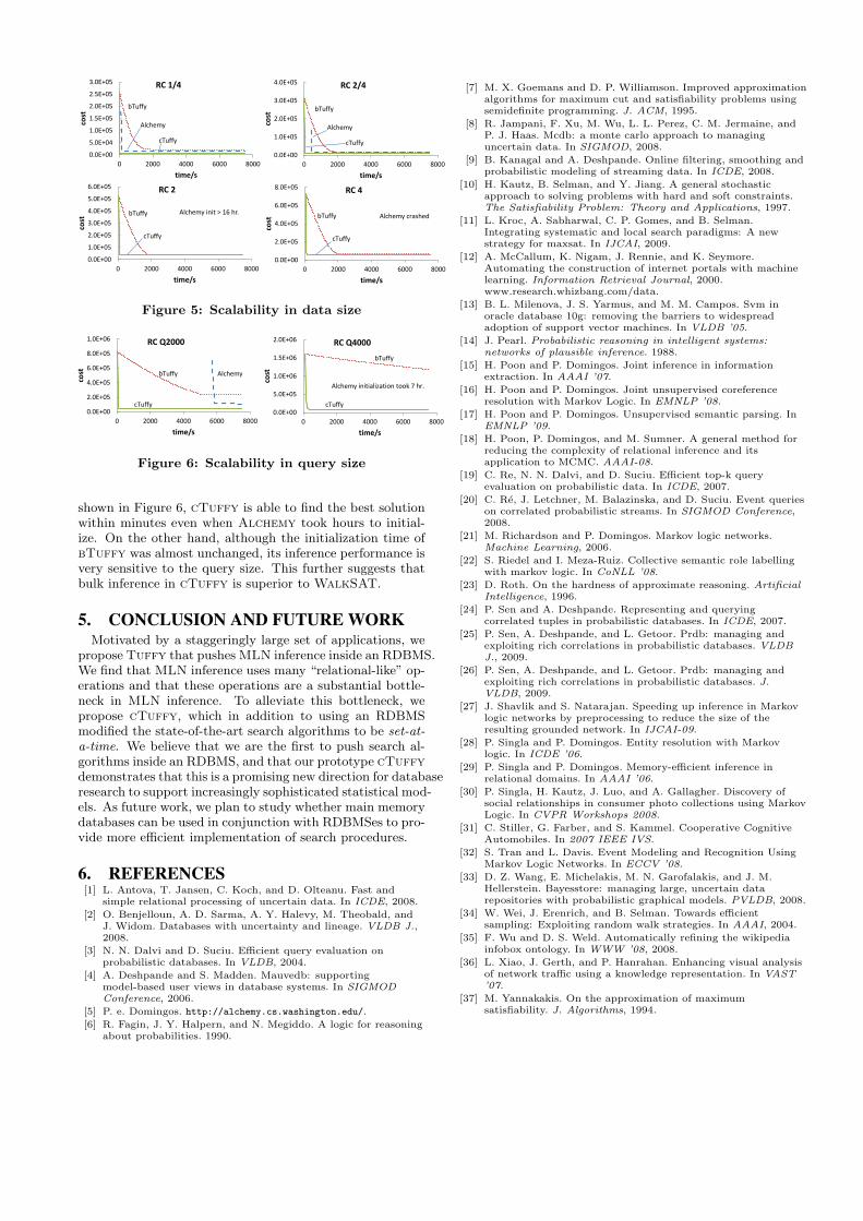
Scalability: Data Size. We compare the scalability of allthree systems with respect to the data size and the querysize. We select RC as the testbed. In Figure 5, we fix thequery size ( i.e., the number of unlabeled papers) to be 1000,and vary the evidence to be random fractions or copies ofthe original dataset. (RCx means the size of the evidence isx times that of RC; e.g., RC2 has twice as many evidenceas RC.) The results show that while bTuffy and cTuffyare very robust to the data size, Alchemy does not scalewell as the the data size grows.

Scalability: Query Size. In a second group of experi-ments, we fix the dataset to be RC, but vary the size ofthe query between 1000 and 4000. (RC Qx means the sizeof the query is x; e.g., RC Q1000 is equivalent to RC,and the query of RC Q2000 contains 2000 papers.) As

9We also conducted a lesion study that separates the con-tributions of these two aspects, see §D.

0.0E+00

5.0E+04

1.0E+05

1.5E+05

2.0E+05

2.5E+05

3.0E+05

0 2000 4000 6000 8000

cost

time/s

RC 1/4

Alchemy

bTuffy

cTuffy

0.0E+00

1.0E+05

2.0E+05

3.0E+05

4.0E+05

5.0E+05

6.0E+05

0 2000 4000 6000 8000

cost

time/s

RC 2

Alchemy init > 16 hr. bTuffy

cTuffy

0.0E+00

2.0E+05

4.0E+05

6.0E+05

8.0E+05

0 2000 4000 6000 8000co

st

time/s

RC 4

Alchemy crashed bTuffy

cTuffy

0.0E+00

1.0E+05

2.0E+05

3.0E+05

4.0E+05

0 2000 4000 6000 8000

cost

time/s

RC 2/4

bTuffy

Alchemy

cTuffy

Figure 5: Scalability in data size

0.0E+00

2.0E+05

4.0E+05

6.0E+05

8.0E+05

1.0E+06

0 2000 4000 6000 8000

cost

time/s

RC Q2000

Alchemy bTuffy

cTuffy 0.0E+00

5.0E+05

1.0E+06

1.5E+06

2.0E+06

0 2000 4000 6000 8000

cost

time/s

RC Q4000

Alchemy initialization took 7 hr.

bTuffy

cTuffy

Figure 6: Scalability in query size

shown in Figure 6, cTuffy is able to find the best solutionwithin minutes even when Alchemy took hours to initial-ize. On the other hand, although the initialization time ofbTuffy was almost unchanged, its inference performance isvery sensitive to the query size. This further suggests thatbulk inference in cTuffy is superior to WalkSAT.

5. CONCLUSION AND FUTURE WORKMotivated by a staggeringly large set of applications, we

propose Tuffy that pushes MLN inference inside an RDBMS.We find that MLN inference uses many “relational-like” op-erations and that these operations are a substantial bottle-neck in MLN inference. To alleviate this bottleneck, wepropose cTuffy, which in addition to using an RDBMSmodified the state-of-the-art search algorithms to be set-at-a-time. We believe that we are the first to push search al-gorithms inside an RDBMS, and that our prototype cTuffydemonstrates that this is a promising new direction for databaseresearch to support increasingly sophisticated statistical mod-els. As future work, we plan to study whether main memorydatabases can be used in conjunction with RDBMSes to pro-vide more efficient implementation of search procedures.

6. REFERENCES[1] L. Antova, T. Jansen, C. Koch, and D. Olteanu. Fast and

simple relational processing of uncertain data. In ICDE, 2008.

[2] O. Benjelloun, A. D. Sarma, A. Y. Halevy, M. Theobald, andJ. Widom. Databases with uncertainty and lineage. VLDB J.,2008.

[3] N. N. Dalvi and D. Suciu. Efficient query evaluation onprobabilistic databases. In VLDB, 2004.

[4] A. Deshpande and S. Madden. Mauvedb: supportingmodel-based user views in database systems. In SIGMODConference, 2006.

[5] P. e. Domingos. http://alchemy.cs.washington.edu/.

[6] R. Fagin, J. Y. Halpern, and N. Megiddo. A logic for reasoningabout probabilities. 1990.

[7] M. X. Goemans and D. P. Williamson. Improved approximationalgorithms for maximum cut and satisfiability problems usingsemidefinite programming. J. ACM, 1995.

[8] R. Jampani, F. Xu, M. Wu, L. L. Perez, C. M. Jermaine, andP. J. Haas. Mcdb: a monte carlo approach to managinguncertain data. In SIGMOD, 2008.

[9] B. Kanagal and A. Deshpande. Online filtering, smoothing andprobabilistic modeling of streaming data. In ICDE, 2008.

[10] H. Kautz, B. Selman, and Y. Jiang. A general stochasticapproach to solving problems with hard and soft constraints.The Satisfiability Problem: Theory and Applications, 1997.

[11] L. Kroc, A. Sabharwal, C. P. Gomes, and B. Selman.Integrating systematic and local search paradigms: A newstrategy for maxsat. In IJCAI, 2009.

[12] A. McCallum, K. Nigam, J. Rennie, and K. Seymore.Automating the construction of internet portals with machinelearning. Information Retrieval Journal, 2000.www.research.whizbang.com/data.

[13] B. L. Milenova, J. S. Yarmus, and M. M. Campos. Svm inoracle database 10g: removing the barriers to widespreadadoption of support vector machines. In VLDB ’05.

[14] J. Pearl. Probabilistic reasoning in intelligent systems:networks of plausible inference. 1988.

[15] H. Poon and P. Domingos. Joint inference in informationextraction. In AAAI ’07.

[16] H. Poon and P. Domingos. Joint unsupervised coreferenceresolution with Markov Logic. In EMNLP ’08.

[17] H. Poon and P. Domingos. Unsupervised semantic parsing. InEMNLP ’09.

[18] H. Poon, P. Domingos, and M. Sumner. A general method forreducing the complexity of relational inference and itsapplication to MCMC. AAAI-08.

[19] C. Re, N. N. Dalvi, and D. Suciu. Efficient top-k queryevaluation on probabilistic data. In ICDE, 2007.

[20] C. Re, J. Letchner, M. Balazinska, and D. Suciu. Event querieson correlated probabilistic streams. In SIGMOD Conference,2008.

[21] M. Richardson and P. Domingos. Markov logic networks.Machine Learning, 2006.

[22] S. Riedel and I. Meza-Ruiz. Collective semantic role labellingwith markov logic. In CoNLL ’08.

[23] D. Roth. On the hardness of approximate reasoning. ArtificialIntelligence, 1996.

[24] P. Sen and A. Deshpande. Representing and queryingcorrelated tuples in probabilistic databases. In ICDE, 2007.

[25] P. Sen, A. Deshpande, and L. Getoor. Prdb: managing andexploiting rich correlations in probabilistic databases. VLDBJ., 2009.

[26] P. Sen, A. Deshpande, and L. Getoor. Prdb: managing andexploiting rich correlations in probabilistic databases. J.VLDB, 2009.

[27] J. Shavlik and S. Natarajan. Speeding up inference in Markovlogic networks by preprocessing to reduce the size of theresulting grounded network. In IJCAI-09.

[28] P. Singla and P. Domingos. Entity resolution with Markovlogic. In ICDE ’06.

[29] P. Singla and P. Domingos. Memory-efficient inference inrelational domains. In AAAI ’06.

[30] P. Singla, H. Kautz, J. Luo, and A. Gallagher. Discovery ofsocial relationships in consumer photo collections using MarkovLogic. In CVPR Workshops 2008.

[31] C. Stiller, G. Farber, and S. Kammel. Cooperative CognitiveAutomobiles. In 2007 IEEE IVS.

[32] S. Tran and L. Davis. Event Modeling and Recognition UsingMarkov Logic Networks. In ECCV ’08.

[33] D. Z. Wang, E. Michelakis, M. N. Garofalakis, and J. M.Hellerstein. Bayesstore: managing large, uncertain datarepositories with probabilistic graphical models. PVLDB, 2008.

[34] W. Wei, J. Erenrich, and B. Selman. Towards efficientsampling: Exploiting random walk strategies. In AAAI, 2004.

[35] F. Wu and D. S. Weld. Automatically refining the wikipediainfobox ontology. In WWW ’08, 2008.

[36] L. Xiao, J. Gerth, and P. Hanrahan. Enhancing visual analysisof network traffic using a knowledge representation. In VAST’07.

[37] M. Yannakakis. On the approximation of maximumsatisfiability. J. Algorithms, 1994.

APPENDIXA. EXTENDED RELATED WORK

The idea of using the stochastic local search algorithmWalkSAT to find the most likely world was due to Kautzet al. [10]. Singla and Domingos [29] extends WalkSATwith lazy materialization in the context of MLNs, result-ing in an algorithm called LazySAT that is used by bothAlchemy and bTuffy. The idea of ignoring ground clausesthat are satisfied by evidence is highlighted as an effectiveway of speeding up the MLN grounding process in Shavlikand Natarajan [27], which formulates the grounding processas nested-loop joins and provides ad hoc heuristics to ap-proximate the optimal join order.

In designing an alternative MAP solver to WalkSAT,Riedel [39] also observed that the grounding process can becast into SQL queries in a straightforward manner. He cor-rectly pointed out that “Database technology is optimisedfor this setting.”

B. SUPPORTING MATERIAL FOR §2

B.1 The Resulting Markov NetworkA Boolean Markov network (or Boolean Markov Random

Field is a model of the joint distribution of a set of Booleanrandom variables X = (X1, . . . , XN ). It is defined by tworelated parts: first, a graph structure G = (X, E); let C de-note the set of cliques in G, then for each C ∈ C there is apotential function denoted φC , which is a function from thevalues of the set of variables in C to non-negative real num-bers. Together, these two pieces define a joint distributionPr(X = x) as follows:

Pr(X = x) =1

Z

YC∈C

φC(xC)

where x ∈ {0, 1}N , Z is a normalization constant and xC

denotes the values of the variables in C.Fix a set of constants C = {c1, . . . , cM}. An MLN de-

fines a Boolean Markov Network as follows: for each pos-sible grounding of each predicate, create a node (and so aBoolean random variable). For example, there will be a noderefers(p1, p2) for each pair of papers p1, p2. For each for-mula Fi we ground it in all possible ways, then we create aclique C that contains the nodes corresponding to all termsin the formula. For example, the key constraint then cre-ates cliques for each paper and all of its potential categories.This feature φi is 1 when its true and 0 when its false; theweight of this feature is wi. We refer to this graph as theground network.

Once we have the ground network, our task reduces toinference in Markov models.

C. SUPPORTING MATERIAL FOR §3

C.1 The LazySAT AlgorithmThe inference algorithm used by Alchemy and bTuffy

is called LazySAT [29]. For completeness, we include itspseudocode here (Algorithm 2). For simplicity, we assumethat all clause weights are positive.

C.2 An Example SQL Query populating theClause Table

Algorithm 2 The LazySAT Algorithm

Input: A: an initial set of atomsInput: C: an initial set of weighted ground clausesInput: MaxFlips, MaxRestartsOutput: σ∗: a truth assignment to A1: lowCost← +∞, σ∗ ← the all-false assignment2: for try = 1 to MaxRestarts do3: σ ← a random truth assignment to A4: for flip = 1 to MaxFlips do5: if cost = 0 then6: return σ∗ // found a solution, halt7: pick a random c ∈ C that’s unsatisfied8: rand← a random float between 0.0 and 1.09: if rand ≤ 0.5 then

10: // a random step11: atomToFlip← a random atom in c

12: else13: // a greedy step14: atomToFlip← an atom in c with lowest δ-cost15: if atomToFlip is inactive then16: A← A ∪ {atomToFlip}17: C ← C∪ ground clauses activated by atomToFlip

18: flip atomToFlip

19: update the cost, as defined in §220: if cost < lowCost then21: lowCost← cost, σ∗ ← σ

Consider the formula F3 in Fig. 1. Suppose that theactual schemata of cat and refers are cat(tid, paper, cat-egory, truth, state) and refers(tid, paper1, paper2, truth,state), respectively. Given the evidence and the current setof active atoms – as indicated by the “truth” and “state” at-tributes – we can ground the active clauses for this formulausing the following SQL query.

SELECT -t1.tid , -t2.tid , t3.tid

FROM cat t1 , refers t2 , cat t3

WHERE (t1.state=ACTIVE OR

(t1.state=EVIDENCE AND t1.truth ))

AND (t2.state=ACTIVE OR

(t2.state=EVIDENCE AND t2.truth ))

AND (t3.state=ACTIVE OR

t3.state=INACTIVE OR

(t3.state=EVIDENCE AND NOT t3.truth ))

AND t1.paper=t2.paper1

AND t1.category=t3.category

AND t2.paper2=t3.paper

Note that the tids of t1 and t2 are negated because thecorresponding predicates are negated in the clausal form ofF3.

C.3 SQL Throughput in bTuffyWe run bTuffy on the datasets described in §4 and mea-

sure the number of SQL queries along the time. In Fig. 7,the monotonically increasing (blue) curve indicates the cu-mulative number of SQL queries that bTuffy has issuedover time; the other (green) one is its derivative, i.e., theRDBMS’s query processing speed. Clearly, as the size ofthe clause table increases, RDBMS’s throughput deterio-rates rapidly. On the most challenging task, ER, Postgrescannot even finish one query (a table scan in effect) within a

0

5

10

15

20

25

30

35

40

45

50

0

20000

40000

60000

80000

100000

120000

140000

0 1000 2000 3000 4000 5000 6000 7000 8000

# q

ue

rie

s/se

c

cum

ula

tive

# q

ue

rie

s

time/s

LP

0

20

40

60

80

100

120

140

160

180

200

0

100000

200000

300000

400000

500000

600000

700000

800000

0 1000 2000 3000 4000 5000 6000 7000 8000

# q

ue

rie

s/se

c

cum

ula

tive

# q

ue

rie

s

time/s

IE

0

0.5

1

1.5

2

2.5

3

3.5

4

4.5

5

0

2000

4000

6000

8000

10000

12000

14000

0 1000 2000 3000 4000 5000 6000 7000 8000

# q

ue

rie

s/se

c

cum

ula

tive

# q

ue

rie

s

time/s

ER

0

5

10

15

20

25

30

35

40

45

50

0

20000

40000

60000

80000

100000

120000

140000

160000

180000

200000

0 1000 2000 3000 4000 5000 6000 7000 8000

# q

ue

rie

s/se

c

cum

ula

tive

# q

ue

rie

s

time/s

RC

Figure 7: SQL throughput in bTuffy

second. An interesting phenomenon from the graph is howthe SQL throughput changes over time. We found that ithas to do with Postgres’s mandatory multi-version concur-rency control (MVCC) component. This further motivatesus to consider in-memory databases as a direction of futurework.

C.4 Computing the Lazy ClosureFor simplicity, we present a relatively naive algorithm to

compute the lazy closure as defined in §3.3 (Algorithm 3).We can naturally derive a semi-naive algorithm, in the samespirit as semi-naive evaluation of Datalog. cTuffy imple-ments a semi-naive algorithm.

Algorithm 3 Precomputing LazySAT Closure

Input: a set of MLN rules with a domain of constantsInput: a database of evidenceOutput: Ac: the closure of active atomsOutput: Gc: the closure of active ground clauses1: Ac ← ∅2: converged← false3: while converged = false do4: G← ground clauses of all rules that are

not satisfied by the evidence,and not satisfied by inactive atoms (those not in Ac)

5: savers← atoms contained in G

6: if savers ⊆ Ac then7: converged← true8: else9: Ac ← Ac ∪ savers

10: Gc ← Gc ∪ G

C.5 Proof of The Closure PropositionProof of Proposition 3.1. Given an MLN, the set of

active ground clauses is a function G of the current set ofactive atoms P . Furthermore, from the definition of G, it’snot hard to see that it is a monotone function: for anyP ⊆ P ′, we have G(P ) ⊆ G(P ′). Let Gx be a set of groundclauses; define E(Gx) to be the set of atoms contained bysome ground clause in Gx. Then the closure algorithm canbe expressed by the initial condition P0 = ∅ and the follow-ing formula:

Pk+1 = Pk ∪ E(Gk+1) = Pk ∪ E(G(Pk)).

0.0E+00

5.0E+04

1.0E+05

1.5E+05

2.0E+05

2.5E+05

3.0E+05

0 500 1000 1500 2000 2500

cost

time (sec)

(b) Benifit of Precomputing Closure (RC**)

bTuffy with Closure

bTuffy

0.0E+00

1.0E+05

2.0E+05

3.0E+05

4.0E+05

5.0E+05

0 500 1000 1500 2000 2500

cost

time (sec)

(a) Benifit of KBMC (RC*)

cTuffy without KBMC

cTuffy

Figure 8: KBMC and Closure precomputation

IE-t RC-twith template loading 9 sec 19 sec

without template loading 16 min 94 min

Figure 9: Initialization time of cTuffy

In Alchemy, the initial set of active atoms is A0 = P0 ⊆P0. Then for k ≥ 1, Ak+1 = Ak ∪ ak+1 where ak+1 is theground atom chosen to be flipped at iteration k + 1. Sinceak+1 ∈ E(G(Ak)), we have Ak+1 ⊆ Ak∪E(G(Ak)). Supposethat Ak ⊆ Pk, then by monotonicity of the functions G andE, Ak+1 ⊆ Pk ∪E(G(Pk)) = Pk+1. By induction, the claimholds.

D. EXTENDED EXPERIMENTSWe discuss several lesion studies to evaluate extensions to

our framework.

Lesion Study: KBMC. cTuffy implements knowledge-based model construction (KBMC) [42], a standard way ofpruning facts and rules that are irrelevant to the query athand. For the purpose of testing, we created a dataset RC*by adding into RC a relation affiliation and a rule that’snot related to cat. As shown in Fig. 8(a), by restrict-ing cTuffy to relevant groundings, KBMC can drasticallyspeed up both initialization and inference.

Lesion Study: Lazy Closure. In §3.3, we described analgorithm to precompute the closure of active groundingsneeded by cTuffy. As it’s very hard to separate this fromthe cTuffy inference algorithm, we conducted a lesion studyon bTuffy instead. To ensure that the initial set of activeatoms does not equal the closure, we removed a non-essentialrule from the MLN of RC, resulting in a task called RC**.As shown in Fig. 8(b), by consolidating all the fine-grainedincremental grounding processes, bTuffy augmented withclosure precomputation can find a solution within half thetime of bTuffy.

Lesion Study: Template Bulk Loading. To single outthe benefit of template bulk loading, we measured the ini-tialization time of cTuffy on two more datasets with thisoptimization enabled and disabled, respectively. The firstdataset, IE-t, is obtained by ten-folding the English wordsin the IE MLN (from thousands to tens of thousands). Thesecond one, RC-t, is derived from RC by replacing x with+x in rule F2 and then instantiating it into individual rules,one for each Person constant.10 As shown in Fig. 9, tem-plate bulk loading can speed up initialization by orders of

10Intuitively, this allows us to model the breadth of study ofindividual researchers.

magnitude.

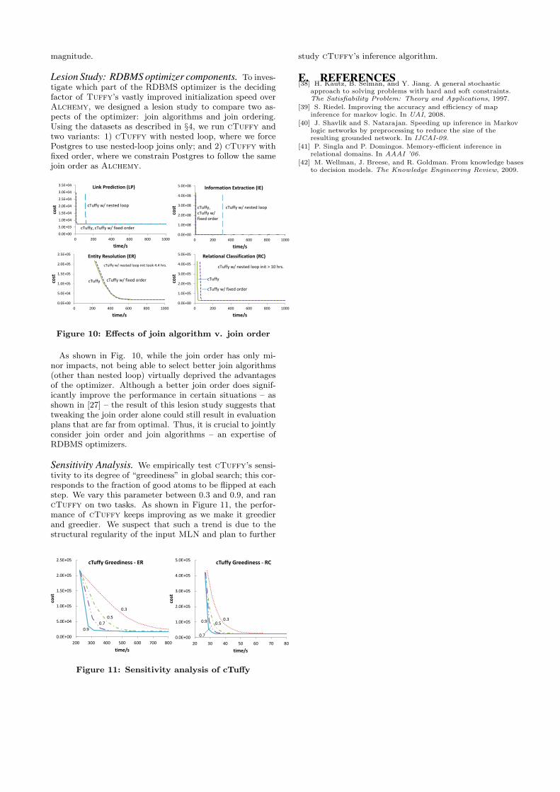
Lesion Study: RDBMS optimizer components. To inves-tigate which part of the RDBMS optimizer is the decidingfactor of Tuffy’s vastly improved initialization speed overAlchemy, we designed a lesion study to compare two as-pects of the optimizer: join algorithms and join ordering.Using the datasets as described in §4, we run cTuffy andtwo variants: 1) cTuffy with nested loop, where we forcePostgres to use nested-loop joins only; and 2) cTuffy withfixed order, where we constrain Postgres to follow the samejoin order as Alchemy.

0.0E+00

5.0E+03

1.0E+04

1.5E+04

2.0E+04

2.5E+04

3.0E+04

3.5E+04

0 200 400 600 800 1000

cost

time/s

Link Prediction (LP)

cTuffy, cTuffy w/ fixed order

cTuffy w/ nested loop

0.0E+00

1.0E+08

2.0E+08

3.0E+08

4.0E+08

5.0E+08

0 200 400 600 800 1000

cost

time/s

Information Extraction (IE)

cTuffy w/ nested loop cTuffy, cTuffy w/ fixed order

0.0E+00

5.0E+04

1.0E+05

1.5E+05

2.0E+05

2.5E+05

0 200 400 600 800 1000

cost

time/s

Entity Resolution (ER)

cTuffy w/ nested loop init took 4.4 hrs.

cTuffy cTuffy w/ fixed order

0.0E+00

1.0E+05

2.0E+05

3.0E+05

4.0E+05

5.0E+05

0 200 400 600 800 1000

cost

time/s

Relational Classification (RC)

cTuffy w/ nested loop init > 10 hrs.

cTuffy

cTuffy w/ fixed order

Figure 10: Effects of join algorithm v. join order

As shown in Fig. 10, while the join order has only mi-nor impacts, not being able to select better join algorithms(other than nested loop) virtually deprived the advantagesof the optimizer. Although a better join order does signif-icantly improve the performance in certain situations – asshown in [27] – the result of this lesion study suggests thattweaking the join order alone could still result in evaluationplans that are far from optimal. Thus, it is crucial to jointlyconsider join order and join algorithms – an expertise ofRDBMS optimizers.

Sensitivity Analysis. We empirically test cTuffy’s sensi-tivity to its degree of “greediness” in global search; this cor-responds to the fraction of good atoms to be flipped at eachstep. We vary this parameter between 0.3 and 0.9, and rancTuffy on two tasks. As shown in Figure 11, the perfor-mance of cTuffy keeps improving as we make it greedierand greedier. We suspect that such a trend is due to thestructural regularity of the input MLN and plan to further

0.0E+00

5.0E+04

1.0E+05

1.5E+05

2.0E+05

2.5E+05

200 300 400 500 600 700 800

cost

time/s

cTuffy Greediness - ER

0.3

0.5

0.7

0.9

0.0E+00

1.0E+05

2.0E+05

3.0E+05

4.0E+05

5.0E+05

20 30 40 50 60 70 80

cost

time/s

cTuffy Greediness - RC

0.3 0.5

0.7

0.9

Figure 11: Sensitivity analysis of cTuffy

study cTuffy’s inference algorithm.

E. REFERENCES[38] H. Kautz, B. Selman, and Y. Jiang. A general stochastic

approach to solving problems with hard and soft constraints.The Satisfiability Problem: Theory and Applications, 1997.

[39] S. Riedel. Improving the accuracy and efficiency of mapinference for markov logic. In UAI, 2008.

[40] J. Shavlik and S. Natarajan. Speeding up inference in Markovlogic networks by preprocessing to reduce the size of theresulting grounded network. In IJCAI-09.

[41] P. Singla and P. Domingos. Memory-efficient inference inrelational domains. In AAAI ’06.

[42] M. Wellman, J. Breese, and R. Goldman. From knowledge basesto decision models. The Knowledge Engineering Review, 2009.