Tuan  V.  Nguyen    Garvan  Ins)tute  of  Medical  Research  

Sydney,  Australia  

Garvan  Ins)tute    Biosta)s)cal  Workshop  16/6/2015   ©  Tuan  V.  Nguyen  

Introduction to linear regression analysis

•  Purposes  

•  Ideas  of  regression    

•  Es)ma)on  of  parameters  

•  R  codes    

 

Purposes of regression analysis

Three types of analysis

•  Analysis  of  difference  

•  Associa)on  analysis  

•  Correla)on  analysis  and  predic)on  

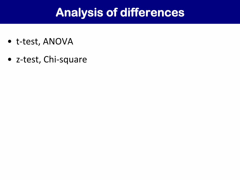
Analysis of differences

•  t-­‐test,  ANOVA  

•  z-­‐test,  Chi-­‐square    

Analysis of association

•  Odds  ra)o    

•  Risk  ra)o  

•  Prevalence  ra)o    

•  etc  

Analysis of correlation

•  Correla)on  analysis  

•  Linear  regression  analysis  

•  Logis)c  regression  

•  Cox's  regression    

•  etc  

A note of history

•  Developed  by  Sir  Francis  Galton  (1822-­‐1911)  in  his  ar)cle  “Regression  towards  mediocrity  in  hereditary  structure”  

Linear regression analysis

•  Assess  /  quan)fy  a  LINEAR  rela)onship  between  variables    

•  Es)mate  the  magnitude  of  effect  of  risk  factors  on  an  outcome  variable    

•  Build  model  of  predic)on    

Purposes of linear regression analysis

•  Find  an  equa)on  to  describe  the  rela)onship  betwee  X  and  Y      

–  X  is  a  predictor,  risk  factor,  independent  variable    –  Y  is  the  outcome  variable,  dependent  variable    

•  Adjustment  for  confounding  factors  

•  Predic)on    

Linear regression model

Ideas of linear regression

How  to  find  an  equa3on  to  link  the  2  poits?    

(x1, y1)

(x2, y2)

x-axis

y-axis

0

Given  two  points  on  a  plane  (x1,  y1)  and  (x2,  y2)  

•  Find  a  slope    

•  Find  the  intercept  (value  of  y  when  x=0)    

(x1, y1)

(x2, y2)

x-axis

y-axis

2 1

2 1

y y yslopex x x

Δ −= =Δ −

0

But we have MANY points ...

x-axis

y-axis

0

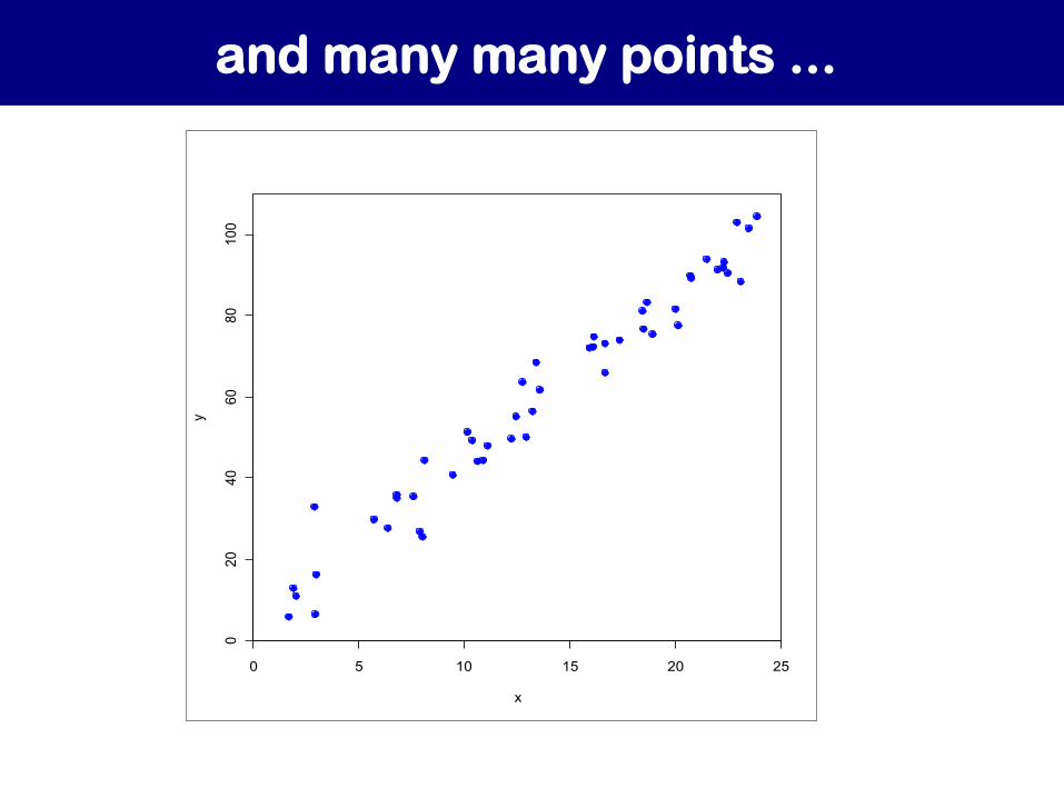
and many many points ...

0 5 10 15 20 25

020

4060

80100

x

y

The linear regression model

•  Simple  linear  regression  model  

•  Y    -­‐  response  variable,  dependent  variable    •  Y  is  a  con)nuous  variable    

•  X    -­‐  predictor  variable,  independent  variable    –  X  can  be  a  con)nuous  variable  or  a  categorical  variable    

 

The linear regression model

 

•  The  statement:    Y  =  α  +  βX  +  ε

α  :  intercept  β  :  slope  /  gradient  

ε  :  random  error  –  the  varia)o  in  Y  for  each  X  value    

•  The  rela)onship  between  X  and  Y  is  linear    

•  X    does  not  have  random  error      

•  Values  of  Y  are  independent  (eg,  Y1  is  not  related  to  Y2)  ;  

•  Random  error  ε:  Normal  distribu)on  with  mean  0,  constant  variance,        

ε  ~  N(0,  σ2)  

Assumptions

Estimation of parameters

Aim of estimation

• The  model  (popula)on):      

 Y  =  α  +  βX  +  ε

• We  don't  know    α  and  β    

• But  we  can  use  observed  data  to  to  es)mate  the  two  parameters  

• Es)mates  of    α  and  β  are  a  and  b    

 

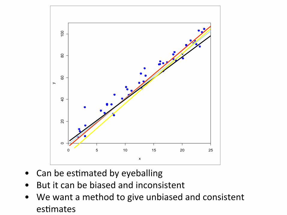
•  Can  be  es)mated  by  eyeballing  •  But  it  can  be  biased  and  inconsistent      •  We  want  a  method  to  give  unbiased  and  consistent  

es)mates    

0 5 10 15 20 25

020

4060

80100

x

y

Criteria for estimation

Y

X

ii bxay +=ˆiii yyd ˆ−=

yi

Find  a  formula  (es)mator)  to  es)mate  a  and  b  so  that  sum  of  d2  is  minimum    à  Least  square  method    

Carl Friedrich Gauss (1777 – 1855)

•  Born  Brunswick,  Germany  

•  Prodigy,  "the  greatest  mathema)cian  since  an)quity"  

•  Inventor  of  the  least  square  method    

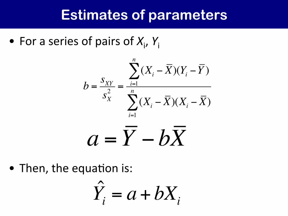
Estimates of parameters

b = sXYsX2 =

(Xi − X)i=1

n

∑ (Yi −Y )

(Xi − X)i=1

n

∑ (Xi − X)

a =Y − bX

•  For  a  series  of  pairs  of  Xi,  Yi    

•  Then,  the  equa)on  is:    

Yi = a+ bXi

Using R

•  The  linear  regression  model:      

Y  =  α  +  β*X  +  ε  

•  R  codes  (using  func)on  lm):    

lm(y ~ x)

Francis Galton's data

•  Galton  F  (1869).  Hereditary  Genius:  An  Inquiry  into  its  Laws  and  Consequences.  London:  Macmillan    

•  Data  from  928  adult  children  born  to  205  fathers  and  mothers  

•  Data  – mid-­‐parent's  height  

–  child's  height  

Galton's data

galton = read.csv("~/Google Drive/Garvan Lectures 2014/Datasets and Teaching Materials/Galton data.csv", header=T)

attach(galton) head(galton) id parent child 1 1 70.5 61.7 2 2 68.5 61.7 3 3 65.5 61.7 4 4 64.5 61.7 5 5 64.0 61.7 6 6 67.5 62.2

64 66 68 70 72

6264

6668

7072

74

parent

child

Linear regression analysis

•  Research  statement:  Child's  height  is  related  to  parent's  height    

•  Sta)s)cal  statement:  

Child  =  α  +  β.Parent  +  ε    

•  R  codes:  m = lm(child ~ parent, data=galton)

 

> m = lm(child ~ parent) > summary(m) Coefficients: Estimate Std. Error t value Pr(>|t|) (Intercept) 23.94153 2.81088 8.517 <2e-16 *** parent 0.64629 0.04114 15.711 <2e-16 *** --- Signif. codes: 0 ‘***’ 0.001 ‘**’ 0.01 ‘*’ 0.05 ‘.’ 0.1 ‘ ’ 1 Residual standard error: 2.239 on 926 degrees of freedom Multiple R-squared: 0.2105, Adjusted R-squared: 0.2096 F-statistic: 246.8 on 1 and 926 DF, p-value: < 2.2e-16

Interpretation of results

Coefficients: Estimate Std. Error t value Pr(>|t|) (Intercept) 23.94153 2.81088 8.517 <2e-16 *** parent 0.64629 0.04114 15.711 <2e-16 ***

•  Remember  that  our  model  is:      

Child  =  a  +  b*Parent  

•  Our  equa)on  is  now:  Child  =  23.94  +  0.646*Parent    

•  Interpreta)on:  Each  in  increase  in  parental  height  is  associated  with  0.64  in  increase  in  child's  height.    

Child = 23.94 + 0.646*Parent

64 66 68 70 72

6264

6668

7072

74

parent

child

Meaning of the regression line

When parental height = 64 in Child = 23.94 + 0.646*64 = 65.3 When parental height = 70 Child = 23.94 + 0.646*70 = 69.2

Expected  value  Child = 23.94 + 0.646*Parent

64 66 68 70 72

6264

6668

7072

74

parent

child

Analysis of variance

Questions concerning linear regression

•  Is  the  model  good  enough?  

• What  criteria  to  judge  the  "goodness  of  fit"?    

•  Good  =  difference  between  observed  and  predicted  values    

Residual (e)

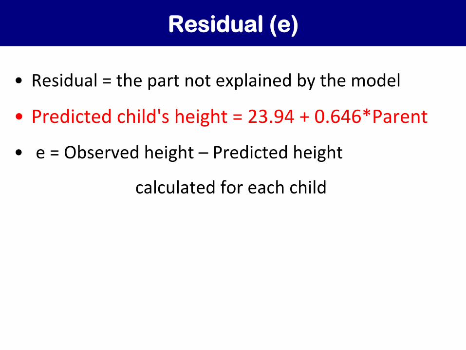
•  Residual  =  the  part  not  explained  by  the  model  

•  Predicted  child's  height  =  23.94  +  0.646*Parent    •   e  =  Observed  height  –  Predicted  height  

calculated  for  each  child    

 

Residual and predicted values using R

m = lm(child ~ parent, data=galton) res = resid(m) pred = predict(m) > cbind(parent, child, pred, res) parent child pred res 1 70.5 61.7 69.50502 -7.80501621 2 68.5 61.7 68.21244 -6.51243505 3 65.5 61.7 66.27356 -4.57356330 4 64.5 61.7 65.62727 -3.92727272 5 64.0 61.7 65.30413 -3.60412743 6 67.5 62.2 67.56614 -5.36614446 7 67.5 62.2 67.56614 -5.36614446 8 67.5 62.2 67.56614 -5.36614446 9 66.5 62.2 66.91985 -4.71985388 10 66.5 62.2 66.91985 -4.71985388 11 66.5 62.2 66.91985 -4.71985388  

Analysis of variance

•  Child  =  a  +  b*Parent  +  e  

•  Observed  varia)on  =  model  +  random  

 “Varia)on”  =  sum  of  squares  

•  SStotal  =  total  sum  of  squares  

 SSreg  =  sum  of  squares  due  to  the  regression  model  

 SSerror  =  sum  of  squares  due  to  random  component  

 

Geometrical representation

Child

Parent

mean

SSR

SSE

SST

SStotal = SSreg + SSerror

Sources of variation

•  Total  SS  =  1237  +  4640  =  5877  – Due  to  "parent":  1236    –  Residuals  (unexplained  part):  4640  

> m = lm(child ~ parent, data=galton) > anova(m)

Analysis of Variance Table Response: child Df Sum Sq Mean Sq F value Pr(>F) parent 1 1236.9 1236.93 246.84 < 2.2e-16 *** Residuals 926 4640.3 5.01 --- Signif. codes: 0 ‘***’ 0.001 ‘**’ 0.01 ‘*’ 0.05 ‘.’ 0.1 ‘ ’ 1

The coefficient of determination (R2)

•  Total  SS  =  1237  +  4640  =  5877  

•  R2  =  1237  /  5877  =  0.21  

> m = lm(child ~ parent, data=galton) > anova(m)

Analysis of Variance Table Response: child Df Sum Sq Mean Sq F value Pr(>F) parent 1 1236.9 1236.93 246.84 < 2.2e-16 *** Residuals 926 4640.3 5.01 --- Signif. codes: 0 ‘***’ 0.001 ‘**’ 0.01 ‘*’ 0.05 ‘.’ 0.1 ‘ ’ 1

Residuals: Min 1Q Median 3Q Max -7.8050 -1.3661 0.0487 1.6339 5.9264 Coefficients: Estimate Std. Error t value Pr(>|t|) (Intercept) 23.94153 2.81088 8.517 <2e-16 *** parent 0.64629 0.04114 15.711 <2e-16 *** --- Signif. codes: 0 ‘***’ 0.001 ‘**’ 0.01 ‘*’ 0.05 ‘.’ 0.1 ‘ ’ 1 Residual standard error: 2.239 on 926 degrees of freedom Multiple R-squared: 0.2105, Adjusted R-squared: 0.2096 F-statistic: 246.8 on 1 and 926 DF, p-value: < 2.2e-16

Meaning of R2

Residual standard error: 2.239 on 926 degrees of freedom Multiple R-squared: 0.2105, Adjusted R-squared: 0.2096 F-statistic: 246.8 on 1 and 926 DF, p-value: < 2.2e-16

•  Coefficient  of  determina)on  R2  =  0.21  

•  Interpreta)on:  Approximately  21%  of  childen's  height  variance  could  be  accounted  for  by  parental  height    

Adjusted R2

•  Defini)on:  

R2adj  =  1  -­‐  (MSerror  /  MStotal)  

MSerror  :  mean  square  due  to  error  

MStotal  :  mean  square  (total)    

Adjusted R2

•  MStotal  =  (1237  +  4640)  /  927  =  6.34  

•  MSerror  =  5  

•  R2adj  =  1  –  (5  /  6.34)  =  0.21  

> m = lm(child ~ parent, data=galton) > anova(m)

Analysis of Variance Table Response: child Df Sum Sq Mean Sq F value Pr(>F) parent 1 1236.9 1236.93 246.84 < 2.2e-16 *** Residuals 926 4640.3 5.01 --- Signif. codes: 0 ‘***’ 0.001 ‘**’ 0.01 ‘*’ 0.05 ‘.’ 0.1 ‘ ’ 1

Residuals: Min 1Q Median 3Q Max -7.8050 -1.3661 0.0487 1.6339 5.9264 Coefficients: Estimate Std. Error t value Pr(>|t|) (Intercept) 23.94153 2.81088 8.517 <2e-16 *** parent 0.64629 0.04114 15.711 <2e-16 *** --- Signif. codes: 0 ‘***’ 0.001 ‘**’ 0.01 ‘*’ 0.05 ‘.’ 0.1 ‘ ’ 1 Residual standard error: 2.239 on 926 degrees of freedom Multiple R-squared: 0.2105, Adjusted R-squared: 0.2096 F-statistic: 246.8 on 1 and 926 DF, p-value: < 2.2e-16

Summary

•  A  simple  linear  regression  model  is  used  to  describe  a  linear  rela)onship  between  two  quan)ta)ve  variables      

•  The  model  allows  es)ma)on  of  effect  size    

•  R  func)on  for  linear  regression:    

lm(y  ~  x)