An offshore Gabon full-waveform inversion case study

Bingmu Xiao1, Nadezhda Kotova1, Samuel Bretherton1, Andrew Ratcliffe1, Gregor Duval1,Chris Page1, and Owen Pape1

Abstract

Velocity model building is one of the most difficult aspects of the seismic processing sequence. But it is alsoone of the most important: an accurate earth model allows an accurate migrated image to be formed, whichallows the geologist a better chance at an accurate interpretation of the area. In addition, the velocity modelitself can provide complementary information about the geology and geophysics of the region. Full-waveforminversion (FWI) is a popular, high-end velocity model-building tool that can generate high-resolution earth mod-els, especially in regions of the model probed by the transmitted (diving wave) arrivals on the recorded seismicdata. The history of the South Gabon Basin is complex, leading to a rich geologic picture today and a verychallenging velocity model-building process. We have developed a case study from the offshore Gabon areashowing that FWI is able to help with the model-building process, and the resulting velocity model reveals fea-tures that improve the migrated image. The application of FWI is made on an extremely large area coveringapproximately 25,000 km2, demonstrating that FWI can be applied to this magnitude of survey in a timely man-ner. In addition, the detail in the FWI velocity model aids the geologic interpretation by highlighting, amongother things, the location of shallow gas pockets, buried channels, and carbonate rafts. The concept of activelyusing the FWI-derived velocity model to aid the interpretation in areas of complex geology, and/or to identifypotential geohazards to avoid in an exploration context, is applicable to many parts of the world.

IntroductionFull-waveform inversion (FWI) offers the potential

to replace the conventional imaging step in seismicprocessing with an inversion for the specific geophysi-cal, or even geological, earth parameter of interest. Itdoes this by attempting to model all of the events in therecorded data — clearly an ambitious target. Althoughthis ultimate objective is still probably many years awaydue to various computational and technical challengesin FWI that are still to be overcome, this topic is atpresent hugely popular in the oil exploration commu-nity in academia and industry. This has been the casefor a number of years since it gained significant momen-tum in the late 2000s following the publication of someimpressive field examples as computing power caughtup with algorithmic complexity. The current paradigmin industrial applications is to use FWI to solve velocitycomplexity in the areas that are well-probed by the div-ing or transmitted waves and derive a velocity modelthat gives uplift in the final migration. This work gener-ally follows this paradigm but with two extra elements:(1) we use the FWI-derived velocity model to aid andoffer additional context to the geologic interpretation

of the seismic image and (2) FWI is applied to anextremely large data set.

The concept of FWI originated more than 30 yearsago with the works of Lailly (1983) and Tarantola(1984). It was significantly ahead of its time with regardto what could be achieved with the computing power ofthe day, meaning even small-scale industrial applica-tions in 3D were beyond its reach. It survived as anactive research topic in academia through the 1990s,particularly with the frequency-domain approach ofPratt (1999) that concentrated specifically on the firstarrival, diving wave energy. Work on the techniqueevolved throughout the 2000s, resulting in some stand-out field-data applications shown in Plessix (2009) andSirgue et al. (2009) among others. Most industrial worksince then has been to establish the robustness of thetechnique, while extending the applicability of themethod with improved technology and improved dataacquisition. Indeed, in a good acquisition geometry forFWI, recording longer offsets and lower frequencies arethe main drivers to give a deeper penetration depth ofthe diving waves and to help alleviate cycle-skippingproblems between the real and modeled synthetic shotgathers (Virieux and Operto, 2009).

1CGG, Crawley, UK. E-mail: bingmu.xiao@cgg.com; nadezhda.kotova@cgg.com; samuel.bretherton@cgg.com; andrew.ratcliffe@cgg.com;gregor.duval@cgg.com; chris.page@cgg.com; owen.pape@cgg.com.

Manuscript received by the Editor 29 February 2016; revised manuscript received 8 July 2016; published online 13 October 2016. This paperappears in Interpretation, Vol. 4, No. 4 (November 2016); p. SU25–SU39, 12 FIGS.

http://dx.doi.org/10.1190/INT-2016-0037.1. © 2016 Society of Exploration Geophysicists and American Association of Petroleum Geologists. All rights reserved.

t

Special section: Applications of full-waveform inversion

Interpretation / November 2016 SU25Interpretation / November 2016 SU25

Dow

nloa

ded

10/1

8/16

to 1

65.2

25.8

0.84

. Red

istr

ibut

ion

subj

ect t

o SE

G li

cens

e or

cop

yrig

ht; s

ee T

erm

s of

Use

at h

ttp://

libra

ry.s

eg.o

rg/

In this paper, we use a data set from offshore Gabonthat was acquired with a broadband, long-offset stream-er profile. We start by outlining the geologic setting ofthe data set before describing the details of the surveyacquisition. The next two sections highlight our FWImethodology and show the FWI results, imaging uplift,and some of the quality control (QC) checks that we do.We then use the resulting seismic image and the FWI-derived velocity model to offer some interpretation ofthe area, with a particular emphasis on the complexitiesin the velocity model arising from the geologic history.We discuss some perspectives on extending the projectbefore concluding. The objective of this work is to showthe potentially exciting step of using information in thevelocity model to aid the geologic interpretation and the

exploration and production development, such as iden-tifying shallow geohazards to avoid when drilling, aswell as highlight the very large areas that can now betackled with FWI.

Geologic settingIn the West Africa Atlantic Margin, one of the last

underexplored regions is the deepwater area of theSouth Gabon Basin. Successful exploration in the conju-gate South Atlantic Margin offshore Brazil has sparkedrenewed interest in deepwater presalt plays in the wholeoffshore southwestern region of Africa, including Gabon,with significant discoveries offshore Angola and Congo,the latter being geographically close to the current sur-vey. Figure 1 shows a generalized stratigraphic column

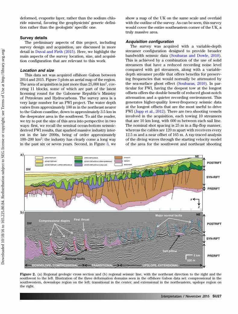
of the area, which shows how the SouthGabon Basin developed in three mainstages: prerift, syn-rift, and postrift. Fig-ure 2a and 2b highlights these stageson a regional geologic cross section andregional seismic line, respectively. Interms of hydrocarbon prospectivity, ex-ploration targets include the deep, highporosity, high permeability, subsalt Bar-remian to Aptian sandstones; the supra-salt Albian-age Madiela carbonate tur-tlebacks; and the Cretaceous Tertiaryturbidite sands that provide establishedtargets further south offshore Angolaand Congo. The diversity of these reser-voir types, and the broad depth range atwhich they are found, means that an ac-curate velocity model is needed to imagethese heterogeneities at all levels of thegeologic section. In terms of structuralcomplexity, the presalt section offers po-tential traps formed by tilted fault blocksand broad rollover anticlines that aresealed by Aptian claystones or salt. Wenote that in the case of the South GabonBasin, these structures need to be im-aged at great depth below the Aptiansalt layer. In the postsalt section, trapscomprise drapes over salt domes andstructural/stratigraphic traps of sand-richchannels within turbidite systems thatare sealed by marine mudstones. In thiscase, we highlight again the necessity ofan accurate velocity model in support ofhigh-resolution broadband seismic to re-solve these thin reservoir beds and strati-graphic pinch-out traps. Of the six wellsthat have been drilled in our 3D surveyarea, only one of them penetrated intothe presalt level, leaving the deeper pro-spectivity in the survey area still an unan-swered question. Finally, we note thatour terminology for “salt” in this paperis to describe any fast velocity, often

Figure 1. Generalized stratigraphic column of the South Gabon basin, with thethree main rift stages highlighted.

SU26 Interpretation / November 2016

Dow

nloa

ded

10/1

8/16

to 1

65.2

25.8

0.84

. Red

istr

ibut

ion

subj

ect t

o SE

G li

cens

e or

cop

yrig

ht; s

ee T

erm

s of

Use

at h

ttp://

libra

ry.s

eg.o

rg/

deformed, evaporite layer, rather than the sodium chlo-ride mineral, favoring the geophysicists’ generic defini-tion rather than the geologists’ specific one.

Survey detailsThe preliminary aspects of this project, including

survey design and acquisition, are discussed in moredetail in Duval and Firth (2015). Here, we highlight themain aspects of the survey location, size, and acquisi-tion configuration that are relevant to this work.

Location and sizeThis data set was acquired offshore Gabon between

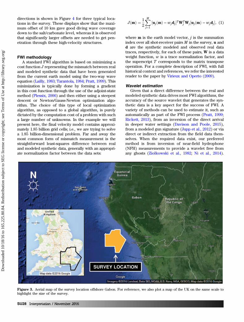
2014 and 2015. Figure 3 plots an aerial map of the region.The area of acquisition is just more than 25,000 km2, cov-ering 11 blocks, some of which are part of the latestlicensing round for the Gabonese Republic’s Ministryof Petroleum and Hydrocarbons. The survey area is avery large number for an FWI project. The water depthvaries from approximately 100 m in the northeast nearerto the Gabon coastline, down to approximately 3.5 km inthe deepwater area in the southwest. To aid the reader,we try to put the size of this area into perspective in twoways: first, we recall the seminal ocean-bottom seismic-derived FWI results, that sparked massive industry inter-est in the late 2000s, being of order approximately100–200 km2: the industry has clearly come a long wayin the past six or seven years. Second, in Figure 3, we

show a map of the UK on the same scale and overlaidwith the outline of the survey. As can be seen, this surveywould cover the entire southeastern corner of the UK, atruly massive area.

Acquisition configurationThe survey was acquired with a variable-depth

streamer configuration designed to provide broaderbandwidth seismic data (Soubaras and Dowle, 2010).This is achieved by a combination of the use of solidstreamers that have a reduced recording noise levelcompared with gel streamers, along with a variable-depth streamer profile that offers benefits for preserv-ing frequencies that would normally be attenuated bythe sea-surface ghost effect (Soubaras, 2010). In par-ticular for FWI, having the deepest tow at the longestoffsets offers the double benefit of reduced ghost-notchattenuation and a quieter recording environment. Thisgenerates higher-quality lower-frequency seismic dataat the longest offsets that are the most useful to driveFWI (Jupp et al., 2012). There are two shooting vesselsinvolved in the acquisition, each towing 10 streamersthat are 10 km long, with 600 m between each sail line.The nominal shot spacing is 25 m in a flip-flop manner,whereas the cables are 120 m apart with receivers every12.5 m and a near offset of 165 m. A ray-traced analysisof the diving waves through the starting velocity modelof the area for the southwest and northeast shooting

Figure 2. (a) Regional geologic cross section and (b) regional seismic line, with the northeast direction to the right and thesouthwest to the left. Illustration of the three deformation domains seen in the offshore Gabon data set: compressional in thesouthwestern, downslope region on the left; transitional in the center; and extensional in the northeastern, upslope region onthe right.

Interpretation / November 2016 SU27

Dow

nloa

ded

10/1

8/16

to 1

65.2

25.8

0.84

. Red

istr

ibut

ion

subj

ect t

o SE

G li

cens

e or

cop

yrig

ht; s

ee T

erm

s of

Use

at h

ttp://

libra

ry.s

eg.o

rg/

directions is shown in Figure 4 for three typical loca-tions in the survey. These displays show that the maxi-mum offset of 10 km gave good diving wave coveragedown to the salt/carbonate level, whereas it is observedthat significantly larger offsets are needed to get pen-etration through these high-velocity structures.

FWI methodologyA standard FWI algorithm is based on minimizing a

cost function J representing the mismatch between realand modeled synthetic data that have been generatedfrom the current earth model using the two-way waveequation (Lailly, 1983; Tarantola, 1984; Pratt, 1999). Thisminimization is typically done by forming a gradientin this cost function through the use of the adjoint-statemethod (Plessix, 2006) and then either using a steepestdescent or Newton/Gauss-Newton optimization algo-rithm. The choice of this type of local optimizationalgorithm, as opposed to a global algorithm, is purelydictated by the computation cost of a problem with sucha large number of unknowns. In the example we willpresent here, the final velocity model contains approxi-mately 1.85 billion grid cells; i.e., we are trying to solvea 1.85 billion-dimensional problem. Far and away themost common form of mismatch measurement is thestraightforward least-squares difference between realand modeled synthetic data, generally with an appropri-ate normalization factor between the data sets:

JðmÞ ¼ 12

XMj¼1

½ujðmÞ −wjdj�TWTj Wj½ujðmÞ −wjdj�; (1)

where m is the earth model vector, j is the summationindex over all shot-receiver pairs M in the survey, u andd are the synthetic modeled and observed real datatraces, respectively, for each of these pairs, W is a dataweight function, w is a trace normalization factor, andthe superscript T corresponds to the matrix transposeoperation. For a complete description of FWI, with fullhistorical context and references, we refer the interestedreader to the paper by Virieux and Operto (2009).

Wavelet estimationGiven that a direct difference between the real and

modeled synthetic data drives most FWI algorithms, theaccuracy of the source wavelet that generates the syn-thetic data is a key aspect for the success of FWI. Avariety of methods can be used to estimate it, such asautomatically as part of the FWI process (Pratt, 1999;Rickett, 2013), from an inversion of the direct arrivalin deeper water settings (Davison and Poole, 2015),from a modeled gun signature (Jupp et al., 2012) or viadirect or indirect extraction from the field data them-selves. When the required data exist, our preferredmethod is from inversion of near-field hydrophone(NFH) measurements to provide a wavelet free fromany ghosts (Ziolkowski et al., 1982; Ni et al., 2014).

Figure 3. Aerial map of the survey location offshore Gabon. For reference, we also plot a map of the UK on the same scale tohighlight the size of the survey.

SU28 Interpretation / November 2016

Dow

nloa

ded

10/1

8/16

to 1

65.2

25.8

0.84

. Red

istr

ibut

ion

subj

ect t

o SE

G li

cens

e or

cop

yrig

ht; s

ee T

erm

s of

Use

at h

ttp://

libra

ry.s

eg.o

rg/

The NFH data were recorded in this survey and, hence,we use this method here.

Data preprocessingWe do not deghost or demultiple the field data and

instead rely on injecting a ghost-free wavelet into a for-ward-modeling process, with a free surface, to generatethe synthetic data (Ratcliffe et al., 2011). In a high-fre-quency imaging process, such a choice of leaving thefree-surface effects in the data would almost certainlylead to crosstalk artifacts in the image caused by spu-rious correlations between primaries and multiples (see,e.g., Wang et al., 2014a). However, in the context of FWI,which is an iterative inversion process, this seems not tobe the case and FWI appears to self-correct crosstalk ar-tifacts from one iteration to the next (Wang et al., 2014b).Although beyond the scope of this paper, we believe thistopic is an interesting one that needsa greater theoretical understanding bythe geophysical community, for example,Chauris and Plessix (2013) and Sun andSymes (2012) discuss this for a similar in-version problem. This workflow has thebenefit of making the preprocessing forFWI a fairly simple procedure, free fromthe often complicated and time consum-ing demultiple and deghosting processes.First, we apply a very low-cut filter to at-tenuate noise below 2 Hz, followed by ahigh-cut filter to 15 Hz with appropriateresampling for more efficient storage ofthe data set for FWI. Although the appli-cation of this high-cut filter clearly limitsthe maximum frequency we can run FWIto, it is not a specific limitation for thework we present here and we can revisitthis step if higher-frequency FWI is re-quired. We then perform basic trace ed-its, swell noise attenuation, and an outerand inner mute to highlight the divingwaves on the shot record.

Velocity updateWe use a time-domain FWI algorithm,

published in detail in Warner et al. (2013)and subsequently updated by Ratcliffeet al. (2014) that is based on the acous-tic wave equation and finite-differencescheme described in Zhang et al. (2011):

1

v20

∂2

∂t2

�p

r

�¼

�1þ 2ε

ffiffiffiffiffiffiffiffiffiffiffiffiffi1þ 2δ

pffiffiffiffiffiffiffiffiffiffiffiffiffi1þ 2δ

p1

�

×� ∂2

∂x2 þ ∂2∂y2 0

0 ∂2∂z2

��p

r

�; (2)

where v0 is the velocity, p is the horizon-tal stress, r is the vertical stress, whereas

ε and δ are the dimensionless anisotropy parameters ofThomsen (1986). The wave equation presented here hasvertical transverse isotropic anisotropy, but can be ex-tended to tilted transverse isotropic (TTI) anisotropywith an appropriate replacement of the spatial differen-tial operators (e.g., see equation 21 in Zhang et al., 2011).Density can be introduced into this wave equation in thestandard manner and is used in this work. The inversionscheme itself is an iterative update to the P-wave velocityvia a linearized least-squares process, using the multi-scale, increasing frequency band, approach of Bunkset al. (1995). In addition, we highlight that the inversionresults presented here do not have any regularizationterms in the cost function of equation 1. Because weuse a time-domain algorithm, whenever we quote a fre-quency for FWI in this paper, we actually refer to thehigh-cut frequency of a low-pass filter, rather than a

Figure 4. Example of a ray-traced diving wave analysis in a shallow-water, car-bonate-dominated, area for: (a) southwest and (b) northeast shooting directions,respectively. Similar analysis is shown in (c) and (d) for a more central, salt-dominated, area, whereas (e) and (f) show a deepwater area from the southwestof the survey. These displays show that the recorded diving waves in the 10 kmstreamer penetrate down to the top-salt/carbonate level.

Interpretation / November 2016 SU29

Dow

nloa

ded

10/1

8/16

to 1

65.2

25.8

0.84

. Red

istr

ibut

ion

subj

ect t

o SE

G li

cens

e or

cop

yrig

ht; s

ee T

erm

s of

Use

at h

ttp://

libra

ry.s

eg.o

rg/

single frequency. Including reflections and transmittedwave energy can be beneficial to FWI in the regions thatare well-probed by the diving waves (Warner et al.,2013). At depths below the level of the diving wave pen-etration, the updates are driven only by reflections. Thevalidity of these perturbations assumes an accuratemacro velocity model at this depth, which varies fromproject to project, and an appropriate density behavior.In this study, we assume a Gardner et al.’s (1974) lawrelationship between density and P-wave velocity, witha smoothly varying modification for water density. Verynice results are obtained when these assumptions arevalid (see, e.g., Kumar et al., 2014). In this project, weacknowledge that uncertainties still exist in the deepervelocity model and, hence, we only use the FWI updatedown to the level of the diving wave penetration, effec-tively the top salt. Overall, this algorithm and methodol-ogy has proved itself on many field data sets withdifferent acquisition types and geometries involvinggeologies from all around the world.

The starting velocity model comes from the currentstage of a larger velocity model-building process downto basement level. Here, FWI is being used as an activecomponent within this larger model build, rather than atthe end of the process as is often seen. At present, thismodel has been built down to the salt level and containsTTI anisotropy that is necessary for the complexityof the region, being derived from a nonlinear slopetomography process (Guillaume et al., 2008). This alsoincluded an update of Thomsen’s (1986) epsilon param-eter in the tomography. Well calibration is not possiblebecause only very limited well data are available in thisregion. Hence, delta is scaled on a layer-by-layer basisaccording to the average epsilon in the layer. The start-ing frequency for FWI was chosen to be 4 Hz by check-ing the data quality at this frequency and confirmingthat the starting model was good enough, such thatcycle skipping was not observed between the real andmodeled synthetic data at this frequency (see the latersubsection on QC). The application here of the classicaldiving-wave-driven FWI using the least-squares data dif-ference needs the underlying kinematics of the startingvelocity model to be accurate to within half a cycle (see,e.g., Virieux and Operto, 2009). The fact that the datawere not observed to be cycle skipped indicates thatthese kinematics are accurate enough to start the inver-sion. The question of the maximum frequency in theFWI is generally a compromise between the observedimprovements in the results as we push to higher fre-quency and the resulting computational cost of obtainingthose results. Given the extremely large area that we areupdating, a value of 8 Hz was chosen as a realistic num-ber. This was based on results obtained from a test swaththat balanced a good observed uplift in the velocitymodel with acceptable runtimes. The interval betweenadjacent frequencies was also tested on this swath(Δf ¼ 1 Hz versus Δf ¼ 2 Hz), and it was found thelarger frequency step gave very similar results to thesmaller one. Hence, the (high-cut) frequencies used in

production were 4, 6, and 8 Hz, with eight iterationsper frequency band and a one-in-eight shot-skippingstrategy per iteration, such shot skipping done on topof any initial shot decimation (see next section).

Spatial sampling and acquisition footprintMost geophysical textbooks discuss the question of

an adequate spatial sampling interval of the wavefieldusing Nyquist-type arguments (see, e.g., Sheriff and Gel-dart, 1995). Ideally, these arguments hold for the shot-and receiver-side sampling in x and y, although on theshot side, it is often thought of as an illumination ques-tion, rather than an aliasing issue. Drawing from thoseworks, we quote that a required spatial sampling inter-val for a plane-wave returning to the surface is

Δ ≤v

2f sin θ; (3)

where Δ is the spatial sampling interval, v is the localvelocity, f is the seismic frequency, and θ is the angle ofthe wavefield with the vertical. In FWI, the cost is di-rectly proportional to the number of shots used,whereas extra receivers within the existing maximumoffset range are effectively computed for free and onlycontribute to the memory and hardware input/output.For typical FWI frequencies of <10 Hz, the receiver sidesampling in x and y is often satisfied by the raw acquis-ition sampling, even in the worst case scenario of awave traveling horizontally. If not, then interpolationbetween the receivers rectifies the situation and addsminimal cost overall. However, on the shot side, weare used to observing a sail-line footprint in the velocitymodel related to the crossline, or y, sampling. This isespecially true in the shallow due to the raw acquisitionspacing between sail lines. Fixing this by interpolatingshots between sail lines is possible, but with direct andsignificant cost implications in the FWI. In most cases,the sail-line footprint in the velocity model can be suc-cessfully attenuated either during or after FWI using asimple processing procedure, as described in Joneset al. (2013), and we apply this here as well. For the il-lumination related to the shot x sampling, in this dataset, we are helped by the deepwater environment and,having obtained a good estimate of the water columnvelocity via other methods, we do not need to updateit with FWI. This means that the shot sampling at thesurface only needs to be good enough to sample energyreturning to the surface at nonhorizontal incidence an-gles, which comes from below the water bottom. Thedeeper the water bottom, the closer toward vertical thisincidence angle will be and, hence, the lower our sam-pling requirements. As an example of this, Figure 5shows a comparison of the raw velocity perturbationsfrom the deepest water area computed from initial shotx samplings of 400 and 800 m, prior to the one-in-eightshot skipping mentioned in the previous section. We seea clear artifact in the 800 m sampled data that disap-pears with a 400 m shot spacing. Given that there are

SU30 Interpretation / November 2016

Dow

nloa

ded

10/1

8/16

to 1

65.2

25.8

0.84

. Red

istr

ibut

ion

subj

ect t

o SE

G li

cens

e or

cop

yrig

ht; s

ee T

erm

s of

Use

at h

ttp://

libra

ry.s

eg.o

rg/

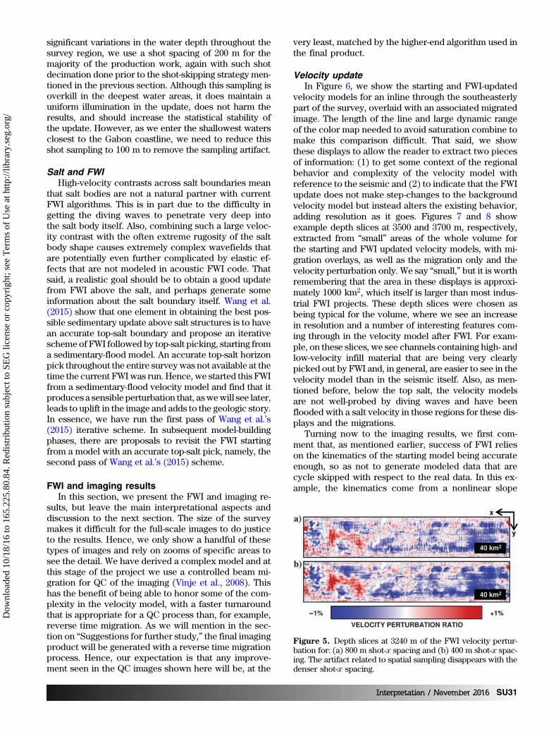
significant variations in the water depth throughout thesurvey region, we use a shot spacing of 200 m for themajority of the production work, again with such shotdecimation done prior to the shot-skipping strategy men-tioned in the previous section. Although this sampling isoverkill in the deepest water areas, it does maintain auniform illumination in the update, does not harm theresults, and should increase the statistical stability ofthe update. However, as we enter the shallowest watersclosest to the Gabon coastline, we need to reduce thisshot sampling to 100 m to remove the sampling artifact.

Salt and FWIHigh-velocity contrasts across salt boundaries mean

that salt bodies are not a natural partner with currentFWI algorithms. This is in part due to the difficulty ingetting the diving waves to penetrate very deep intothe salt body itself. Also, combining such a large veloc-ity contrast with the often extreme rugosity of the saltbody shape causes extremely complex wavefields thatare potentially even further complicated by elastic ef-fects that are not modeled in acoustic FWI code. Thatsaid, a realistic goal should be to obtain a good updatefrom FWI above the salt, and perhaps generate someinformation about the salt boundary itself. Wang et al.(2015) show that one element in obtaining the best pos-sible sedimentary update above salt structures is to havean accurate top-salt boundary and propose an iterativescheme of FWI followed by top-salt picking, starting froma sedimentary-flood model. An accurate top-salt horizonpick throughout the entire surveywas not available at thetime the current FWIwas run. Hence, we started this FWIfrom a sedimentary-flood velocity model and find that itproduces a sensible perturbation that, aswewill see later,leads to uplift in the image and adds to the geologic story.In essence, we have run the first pass of Wang et al.’s(2015) iterative scheme. In subsequent model-buildingphases, there are proposals to revisit the FWI startingfrom a model with an accurate top-salt pick, namely, thesecond pass of Wang et al.’s (2015) scheme.

FWI and imaging resultsIn this section, we present the FWI and imaging re-

sults, but leave the main interpretational aspects anddiscussion to the next section. The size of the surveymakes it difficult for the full-scale images to do justiceto the results. Hence, we only show a handful of thesetypes of images and rely on zooms of specific areas tosee the detail. We have derived a complex model and atthis stage of the project we use a controlled beam mi-gration for QC of the imaging (Vinje et al., 2008). Thishas the benefit of being able to honor some of the com-plexity in the velocity model, with a faster turnaroundthat is appropriate for a QC process than, for example,reverse time migration. As we will mention in the sec-tion on “Suggestions for further study,” the final imagingproduct will be generated with a reverse time migrationprocess. Hence, our expectation is that any improve-ment seen in the QC images shown here will be, at the

very least, matched by the higher-end algorithm used inthe final product.

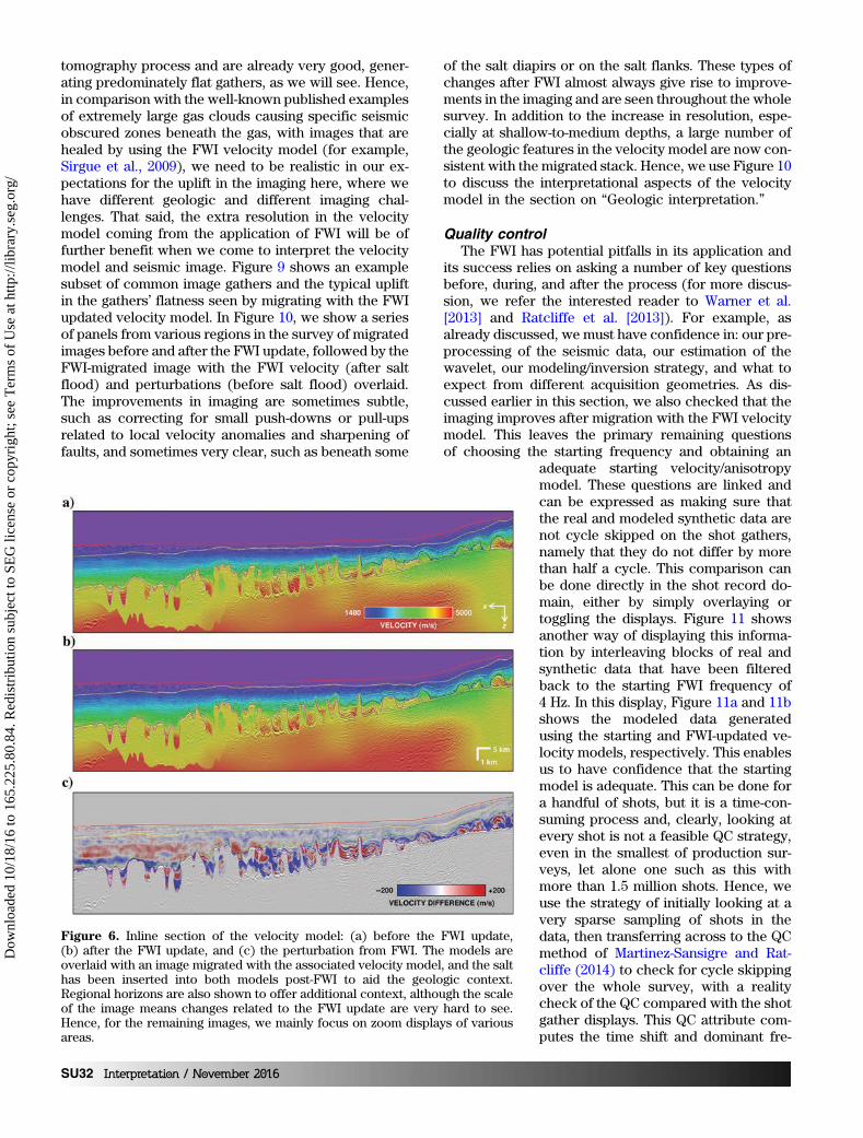
Velocity updateIn Figure 6, we show the starting and FWI-updated

velocity models for an inline through the southeasterlypart of the survey, overlaid with an associated migratedimage. The length of the line and large dynamic rangeof the color map needed to avoid saturation combine tomake this comparison difficult. That said, we showthese displays to allow the reader to extract two piecesof information: (1) to get some context of the regionalbehavior and complexity of the velocity model withreference to the seismic and (2) to indicate that the FWIupdate does not make step-changes to the backgroundvelocity model but instead alters the existing behavior,adding resolution as it goes. Figures 7 and 8 showexample depth slices at 3500 and 3700 m, respectively,extracted from “small” areas of the whole volume forthe starting and FWI updated velocity models, with mi-gration overlays, as well as the migration only and thevelocity perturbation only. We say “small,” but it is worthremembering that the area in these displays is approxi-mately 1000 km2, which itself is larger than most indus-trial FWI projects. These depth slices were chosen asbeing typical for the volume, where we see an increasein resolution and a number of interesting features com-ing through in the velocity model after FWI. For exam-ple, on these slices, we see channels containing high- andlow-velocity infill material that are being very clearlypicked out by FWI and, in general, are easier to see in thevelocity model than in the seismic itself. Also, as men-tioned before, below the top salt, the velocity modelsare not well-probed by diving waves and have beenflooded with a salt velocity in those regions for these dis-plays and the migrations.

Turning now to the imaging results, we first com-ment that, as mentioned earlier, success of FWI relieson the kinematics of the starting model being accurateenough, so as not to generate modeled data that arecycle skipped with respect to the real data. In this ex-ample, the kinematics come from a nonlinear slope

Figure 5. Depth slices at 3240 m of the FWI velocity pertur-bation for: (a) 800 m shot-x spacing and (b) 400 m shot-x spac-ing. The artifact related to spatial sampling disappears with thedenser shot-x spacing.

Interpretation / November 2016 SU31

Dow

nloa

ded

10/1

8/16

to 1

65.2

25.8

0.84

. Red

istr

ibut

ion

subj

ect t

o SE

G li

cens

e or

cop

yrig

ht; s

ee T

erm

s of

Use

at h

ttp://

libra

ry.s

eg.o

rg/

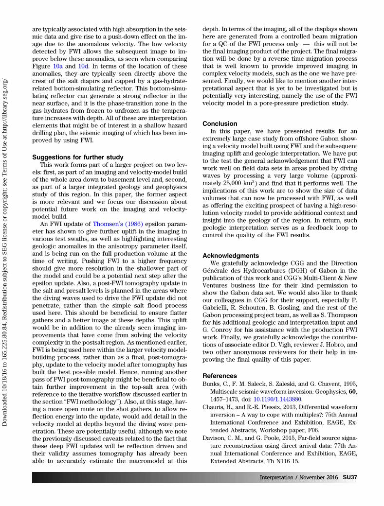
tomography process and are already very good, gener-ating predominately flat gathers, as we will see. Hence,in comparison with the well-known published examplesof extremely large gas clouds causing specific seismicobscured zones beneath the gas, with images that arehealed by using the FWI velocity model (for example,Sirgue et al., 2009), we need to be realistic in our ex-pectations for the uplift in the imaging here, where wehave different geologic and different imaging chal-lenges. That said, the extra resolution in the velocitymodel coming from the application of FWI will be offurther benefit when we come to interpret the velocitymodel and seismic image. Figure 9 shows an examplesubset of common image gathers and the typical upliftin the gathers’ flatness seen by migrating with the FWIupdated velocity model. In Figure 10, we show a seriesof panels from various regions in the survey of migratedimages before and after the FWI update, followed by theFWI-migrated image with the FWI velocity (after saltflood) and perturbations (before salt flood) overlaid.The improvements in imaging are sometimes subtle,such as correcting for small push-downs or pull-upsrelated to local velocity anomalies and sharpening offaults, and sometimes very clear, such as beneath some

of the salt diapirs or on the salt flanks. These types ofchanges after FWI almost always give rise to improve-ments in the imaging and are seen throughout the wholesurvey. In addition to the increase in resolution, espe-cially at shallow-to-medium depths, a large number ofthe geologic features in the velocity model are now con-sistent with the migrated stack. Hence, we use Figure 10to discuss the interpretational aspects of the velocitymodel in the section on “Geologic interpretation.”

Quality controlThe FWI has potential pitfalls in its application and

its success relies on asking a number of key questionsbefore, during, and after the process (for more discus-sion, we refer the interested reader to Warner et al.[2013] and Ratcliffe et al. [2013]). For example, asalready discussed, we must have confidence in: our pre-processing of the seismic data, our estimation of thewavelet, our modeling/inversion strategy, and what toexpect from different acquisition geometries. As dis-cussed earlier in this section, we also checked that theimaging improves after migration with the FWI velocitymodel. This leaves the primary remaining questionsof choosing the starting frequency and obtaining an

adequate starting velocity/anisotropymodel. These questions are linked andcan be expressed as making sure thatthe real and modeled synthetic data arenot cycle skipped on the shot gathers,namely that they do not differ by morethan half a cycle. This comparison canbe done directly in the shot record do-main, either by simply overlaying ortoggling the displays. Figure 11 showsanother way of displaying this informa-tion by interleaving blocks of real andsynthetic data that have been filteredback to the starting FWI frequency of4 Hz. In this display, Figure 11a and 11bshows the modeled data generatedusing the starting and FWI-updated ve-locity models, respectively. This enablesus to have confidence that the startingmodel is adequate. This can be done fora handful of shots, but it is a time-con-suming process and, clearly, looking atevery shot is not a feasible QC strategy,even in the smallest of production sur-veys, let alone one such as this withmore than 1.5 million shots. Hence, weuse the strategy of initially looking at avery sparse sampling of shots in thedata, then transferring across to the QCmethod of Martinez-Sansigre and Rat-cliffe (2014) to check for cycle skippingover the whole survey, with a realitycheck of the QC compared with the shotgather displays. This QC attribute com-putes the time shift and dominant fre-

Figure 6. Inline section of the velocity model: (a) before the FWI update,(b) after the FWI update, and (c) the perturbation from FWI. The models areoverlaid with an image migrated with the associated velocity model, and the salthas been inserted into both models post-FWI to aid the geologic context.Regional horizons are also shown to offer additional context, although the scaleof the image means changes related to the FWI update are very hard to see.Hence, for the remaining images, we mainly focus on zoom displays of variousareas.

SU32 Interpretation / November 2016

Dow

nloa

ded

10/1

8/16

to 1

65.2

25.8

0.84

. Red

istr

ibut

ion

subj

ect t

o SE

G li

cens

e or

cop

yrig

ht; s

ee T

erm

s of

Use

at h

ttp://

libra

ry.s

eg.o

rg/

quency in the data, then, together with error estimatesin these quantities, computes an estimate of the prob-ability of cycle skipping between real and modeled syn-thetic data. Figure 12 shows an example of this process,where we consider a subset of the shot gathers, namelyone every 10 km and every 10th sail line. We generate aQC attribute value for each seismic trace in the shotgather and plot it in an aerial sense using the tracereceiver x and y. Again, we have to zoom into a specificregion to see the detail. As a rule of thumb, we choosethe 5% probability level as a threshold for starting to beconcerned by cycle skipping. The before and after FWIdisplays shown in Figure 12a and 12b, respectively,highlight that the starting model is, in general, not cycleskipped and that the vast majority of the cycle skippingis reduced, or entirely removed, after application ofFWI. The odd pocket remains here and there, flaggingareas to look at in more detail. The small regions of po-tential cycle skipping on the starting model are mostoften seen in the nearest offsets, rather than at the far.This is slightly surprising because, if this was true cycleskipping, then we would expect it to be flagged in multi-ple regions on the gather. Our interpretation is that thisis due to remaining low-frequency noise in the seismicdata that is biasing the QC in this region.

Geologic interpretationThe formation of the South Gabon basin started in

Early Cretaceous times with the opening of the SouthAtlantic rift. During this time, the deposited fluvial andlacustrine type continental sediments now form today’sprimary hydrocarbon source and reservoirs rocks —

these are the main targets at depths of more than4000 m in the survey area. In later Aptian times, aridclimate conditions prevailed with high evaporationrates and a salt layer was deposited as sea waters pro-gressively made their way through the area. Figure 2shows that, following a period of halokinesis, this saltis now heavily deformed. However, it still forms a majortop seal across the basin, stopping and trapping hydro-carbons below in the Aptian reservoir sands. On a basinscale, helped by the ocean-ward tilt of the West Africamargin, the sediments overlying the salt slid downslope,with the salt acting like a regional detachment layer toaid the sliding process. This gave rise to the formationof a large-scale gravitational gliding complex over tensof thousands of square kilometers and resulted in verycomplex salt structures with many diapirs, thrusts, andcanopies forming in the section. Other sources of com-plexity are the remaining pieces of the broken-up Al-bian carbonate shelf that are now sliding on the salt.

Figure 7. Depth slices at 3500 m for: (a) starting velocity model, (b) FWI velocity model, (c) seismic image migrated with FWI-velocity model, and (d) the velocity perturbation. The inset in (c) shows the approximately 1000 km2 displayed area relative to thefull area of the survey.

Interpretation / November 2016 SU33

Dow

nloa

ded

10/1

8/16

to 1

65.2

25.8

0.84

. Red

istr

ibut

ion

subj

ect t

o SE

G li

cens

e or

cop

yrig

ht; s

ee T

erm

s of

Use

at h

ttp://

libra

ry.s

eg.o

rg/

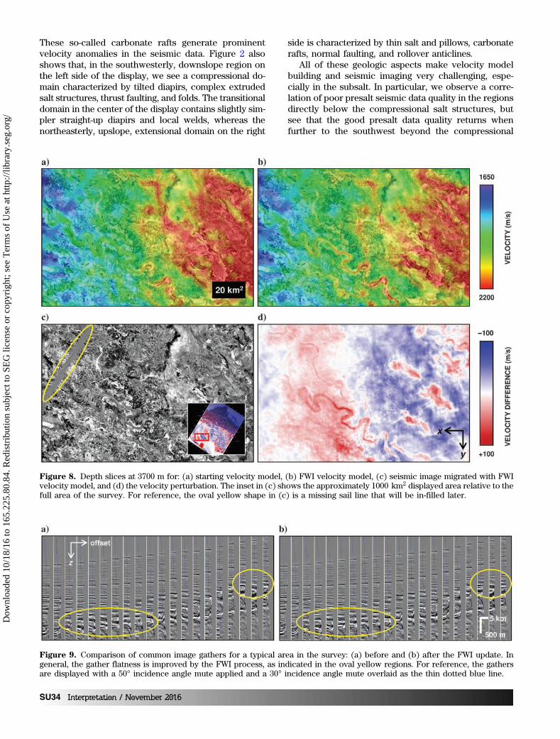
These so-called carbonate rafts generate prominentvelocity anomalies in the seismic data. Figure 2 alsoshows that, in the southwesterly, downslope region onthe left side of the display, we see a compressional do-main characterized by tilted diapirs, complex extrudedsalt structures, thrust faulting, and folds. The transitionaldomain in the center of the display contains slightly sim-pler straight-up diapirs and local welds, whereas thenortheasterly, upslope, extensional domain on the right

side is characterized by thin salt and pillows, carbonaterafts, normal faulting, and rollover anticlines.

All of these geologic aspects make velocity modelbuilding and seismic imaging very challenging, espe-cially in the subsalt. In particular, we observe a corre-lation of poor presalt seismic data quality in the regionsdirectly below the compressional salt structures, butsee that the good presalt data quality returns whenfurther to the southwest beyond the compressional

Figure 8. Depth slices at 3700 m for: (a) starting velocity model, (b) FWI velocity model, (c) seismic image migrated with FWIvelocity model, and (d) the velocity perturbation. The inset in (c) shows the approximately 1000 km2 displayed area relative to thefull area of the survey. For reference, the oval yellow shape in (c) is a missing sail line that will be in-filled later.

Figure 9. Comparison of common image gathers for a typical area in the survey: (a) before and (b) after the FWI update. Ingeneral, the gather flatness is improved by the FWI process, as indicated in the oval yellow regions. For reference, the gathersare displayed with a 50° incidence angle mute applied and a 30° incidence angle mute overlaid as the thin dotted blue line.

SU34 Interpretation / November 2016

Dow

nloa

ded

10/1

8/16

to 1

65.2

25.8

0.84

. Red

istr

ibut

ion

subj

ect t

o SE

G li

cens

e or

cop

yrig

ht; s

ee T

erm

s of

Use

at h

ttp://

libra

ry.s

eg.o

rg/

Figure 10. Examples from throughout the survey of the imaging: (a-c) before and (d-f) after the FWI update. The updated velocitymodel with the additional post-FWI salt flood is shown as an overlay in (g-i). Panels (j-l) and (m-o) show the raw FWI perturbation(before salt flood) with and without the top salt mute, respectively.

Interpretation / November 2016 SU35

Dow

nloa

ded

10/1

8/16

to 1

65.2

25.8

0.84

. Red

istr

ibut

ion

subj

ect t

o SE

G li

cens

e or

cop

yrig

ht; s

ee T

erm

s of

Use

at h

ttp://

libra

ry.s

eg.o

rg/

domain (not shown for reasons of space). Lookingagain at Figure 10, this shows zoomed-in displays fromthroughout the survey of the migrated seismic beforeand after the FWI update, for an example of each ofthese three domains: compressional in the left column,transitional in the middle column, and extensional inthe right column. In one row on this figure, we also plotthe FWI velocity model overlaid with the migrated sec-tion, as well as the perturbation with and without thetop-salt mute, to highlight these features on the velocitymodel, thus aiding and reinforcing the interpretation.For example, Figure 10i shows that the FWI model

nicely delineated the carbonate rafts, which have afaster velocity than the salt bodies here, with a slow-fast-slow internal structure. At the base salt level, priorto the FWI update, we see velocity pull-ups where thecarbonate rafts are present and push-downs where theyare absent and replaced by salt pillows. Comparingthe displays in Figure 10c and 10f, we see that these dis-tortions are improved when migrating with the FWIvelocity model (recall that the FWI update did not sig-nificantly penetrate into the salt itself and that part ofthe model is subsequently replaced with a salt flood inthese migrations). Also, we see that the location of thetop-salt reflectors, and associated sharp velocity in-crease, are generally well-captured by FWI (see, e.g.,the salt diapirs on the unmuted FWI perturbation in Fig-ure 10m), although we note that we ended up mutingthis out and flooding for the reasons discussed earlier.Figure 10g and 10j highlights (white oval) where one ofthe sand channels above the salt/carbonate region isvisible with a lower velocity than the surrounding sedi-ments (the type of features seen in the depth slices ofFigures 7 and 8). These types of channel features arevery visible in the FWI velocity model and prevalentthroughout the survey. If we now turn our attentionto the shallower part of the section in Figure 10d and10g, the first few 100 m of the near-surface Pliocene-Pleistocene section are known to be affected by polygo-nal faulting. This is indicative that these sediments arevery unconsolidated and actively dewatering at pres-ent. This means they still contain large volumes ofwater, giving rise to a very low interval velocity (closeto water velocity) that is visible in the very shallow partof the velocity display in Figure 10g. In this part of thesection, we also see evidence for gas escape conduits inthe seismic image and FWI velocity model (indicated inFigure 10l). Additionally, we are able to identify shallowbright amplitude packets (Figure 10d) as slow velocitygas pockets in the velocity model (Figure 10j, blackovals). These sharp, localized, low-velocity “bubbles”

Figure 11. The QC of interleaved blocks of real and modeledsynthetic data filtered to 4 Hz: (a) before and (b) after the FWIupdate.

Figure 12. The QC showing the probability of cycle-skipping attribute evaluated at 4 Hz: (a) before and (b) after the FWI update.This display shows data for a shot pattern every 10 km along the sail line and every 10th sail line. This display can be repeated forthe different frequency bands as the inversion proceeds.

SU36 Interpretation / November 2016

Dow

nloa

ded

10/1

8/16

to 1

65.2

25.8

0.84

. Red

istr

ibut

ion

subj

ect t

o SE

G li

cens

e or

cop

yrig

ht; s

ee T

erm

s of

Use

at h

ttp://

libra

ry.s

eg.o

rg/

are typically associated with high absorption in the seis-mic data and give rise to a push-down effect on the im-age due to the anomalous velocity. The low velocitydetected by FWI allows the subsequent image to im-prove below these anomalies, as seen when comparingFigure 10a and 10d. In terms of the location of theseanomalies, they are typically seen directly above thecrest of the salt diapirs and capped by a gas-hydrate-related bottom-simulating reflector. This bottom-simu-lating reflector can generate a strong reflector in thenear surface, and it is the phase-transition zone in thegas hydrates from frozen to unfrozen as the tempera-ture increases with depth. All of these are interpretationelements that might be of interest in a shallow hazarddrilling plan, the seismic imaging of which has been im-proved by using FWI.

Suggestions for further studyThis work forms part of a larger project on two lev-

els: first, as part of an imaging and velocity-model buildof the whole area down to basement level and, second,as part of a larger integrated geology and geophysicsstudy of this region. In this paper, the former aspectis more relevant and we focus our discussion aboutpotential future work on the imaging and velocity-model build.

An FWI update of Thomsen’s (1986) epsilon param-eter has shown to give further uplift in the imaging invarious test swaths, as well as highlighting interestinggeologic anomalies in the anisotropy parameter itself,and is being run on the full production volume at thetime of writing. Pushing FWI to a higher frequencyshould give more resolution in the shallower part ofthe model and could be a potential next step after theepsilon update. Also, a post-FWI tomography update inthe salt and presalt levels is planned in the areas wherethe diving waves used to drive the FWI update did notpenetrate, rather than the simple salt flood processused here. This should be beneficial to ensure flattergathers and a better image at these depths. This upliftwould be in addition to the already seen imaging im-provements that have come from solving the velocitycomplexity in the postsalt region. As mentioned earlier,FWI is being used here within the larger velocity model-building process, rather than as a final, post-tomogra-phy, update to the velocity model after tomography hasbuilt the best possible model. Hence, running anotherpass of FWI post-tomography might be beneficial to ob-tain further improvement in the top-salt area (withreference to the iterative workflow discussed earlier inthe section “FWImethodology”). Also, at this stage, hav-ing a more open mute on the shot gathers, to allow re-flection energy into the update, would add detail in thevelocity model at depths beyond the diving wave pen-etration. These are potentially useful, although we notethe previously discussed caveats related to the fact thatthese deep FWI updates will be reflection driven andtheir validity assumes tomography has already beenable to accurately estimate the macromodel at this

depth. In terms of the imaging, all of the displays shownhere are generated from a controlled beam migrationfor a QC of the FWI process only — this will not bethe final imaging product of the project. The final migra-tion will be done by a reverse time migration processthat is well known to provide improved imaging incomplex velocity models, such as the one we have pre-sented. Finally, we would like to mention another inter-pretational aspect that is yet to be investigated but ispotentially very interesting, namely the use of the FWIvelocity model in a pore-pressure prediction study.

ConclusionIn this paper, we have presented results for an

extremely large case study from offshore Gabon show-ing a velocity model built using FWI and the subsequentimaging uplift and geologic interpretation. We have putto the test the general acknowledgement that FWI canwork well on field data sets in areas probed by divingwaves by processing a very large volume (approxi-mately 25,000 km2) and find that it performs well. Theimplications of this work are to show the size of datavolumes that can now be processed with FWI, as wellas offering the exciting prospect of having a high-reso-lution velocity model to provide additional context andinsight into the geology of the region. In return, suchgeologic interpretation serves as a feedback loop tocontrol the quality of the FWI results.

AcknowledgmentsWe gratefully acknowledge CGG and the Direction

Générale des Hydrocarbures (DGH) of Gabon in thepublication of this work and CGG’s Multi-Client & NewVentures business line for their kind permission toshow the Gabon data set. We would also like to thankour colleagues in CGG for their support, especially P.Gabrielli, R. Schouten, B. Gosling, and the rest of theGabon processing project team, as well as S. Thompsonfor his additional geologic and interpretation input andG. Conroy for his assistance with the production FWIwork. Finally, we gratefully acknowledge the contribu-tions of associate editor D. Vigh, reviewer J. Hobro, andtwo other anonymous reviewers for their help in im-proving the final quality of this paper.

ReferencesBunks, C., F. M. Saleck, S. Zaleski, and G. Chavent, 1995,

Multiscale seismic waveform inversion: Geophysics, 60,1457–1473, doi: 10.1190/1.1443880.

Chauris, H., and R.-E. Plessix, 2013, Differential waveforminversion – A way to cope with multiples?: 75th AnnualInternational Conference and Exhibition, EAGE, Ex-tended Abstracts, Workshop paper, F06.

Davison, C. M., and G. Poole, 2015, Far-field source signa-ture reconstruction using direct arrival data: 77th An-nual International Conference and Exhibition, EAGE,Extended Abstracts, Th N116 15.

Interpretation / November 2016 SU37

Dow

nloa

ded

10/1

8/16

to 1

65.2

25.8

0.84

. Red

istr

ibut

ion

subj

ect t

o SE

G li

cens

e or

cop

yrig

ht; s

ee T

erm

s of

Use

at h

ttp://

libra

ry.s

eg.o

rg/

Duval, G., and J. Firth, 2015, G&G integration enhances ac-quisition of multi-client studies offshore Gabon: WorldOil, July, 57–61.

Gardner, G. H. F., L. W. Gardner, and A. R. Gregory, 1974,Formation velocity and density—The diagnostic basicsfor stratigraphic traps: Geophysics, 39, 770–780, doi: 10.1190/1.1440465.

Guillaume, P., G. Lambaré, O. Leblanc, P. Mitouard, J. LeMoigne, J.-P. Montel, T. Prescott, R. Siliqi, N. Vidal,X. Zhang, and S. Zimine, 2008, Kinematic invariants:An efficient and flexible approach for velocity modelbuilding: 78th Annual International Meeting, SEG, Ex-panded Abstracts, 3687–3692.

Jones, C. E., M. Evans, A. Ratcliffe, G. Conroy, R. Jupp, J. I.Selvage, and L. Ramsey, 2013, Full waveform inversionin a complex geological setting: A narrow azimuthtowed streamer case study from the Barents sea: 75thAnnual International Conference and Exhibition,EAGE, Extended Abstracts, We 11 06.

Jupp, R., A. Ratcliffe, and R. Wombell, 2012, Applicationof full waveform inversion to variable-depth streamerdata: 82nd Annual International Meeting, SEG, Ex-panded Abstracts, doi: 10.1190/segam2012-0613.1.

Kumar, R., B. Bai, and Y. Huang, 2014, Using reflection datafor full waveform inversion: A case study from SantosBasin, Brazil: 76th Annual International Conference andExhibition, EAGE, Extended Abstracts, Th E106 15.

Lailly, P., 1983, The seismic inverse problem as a sequenceof before stack migrations: Proceedings of the Inter-national Conference on Inverse Scattering, Theory,and Applications: SIAM.

Martinez-Sansigre, A., and A. Ratcliffe, 2014, A probabilis-tic QC for cycle-skipping in full waveform inversion:84th Annual International Meeting, SEG, Expanded Ab-stracts, 1105–1109.

Ni, Y., T. Payen, and A. Vesin, 2014, Joint inversion of near-field and far-field hydrophone data for source signatureestimation: 84th Annual International Meeting, SEG, Ex-panded Abstracts, 57–61.

Plessix, R.-E., 2006, A review of the adjoint-state method forcomputing the gradient of a functional with geophysicalapplications: Geophysical Journal International, 167,495–503, doi: 10.1111/j.1365-246X.2006.02978.x.

Plessix, R.-E., 2009, Three-dimensional frequency-domainfull-waveform inversionwith an iterative solver: Geophys-ics, 74, no. 6, WCC149–WCC157, doi: 10.1190/1.3211198.

Pratt, R. G., 1999, Seismic waveform inversion in the fre-quency domain. Part 1: Theory and verification in aphysical scale model: Geophysics, 64, 888–901, doi:10.1190/1.1444597.

Ratcliffe, A., A. Karagul, C. Henstock, G. Conroy, and V.Vinje, 2013, QC of full waveform inversion: 75th AnnualInternational Conference and Exhibition, EAGE, Ex-tended Abstracts, Workshop paper, A03.

Ratcliffe, A., A. Privitera, G. Conroy, V. Vinje, A. Bertrand,and B. Lyngnes, 2014, Enhanced imaging with high-resolution full-waveform inversion and reverse time

migration: A North Sea OBC case study: The LeadingEdge, 33, 986–992, doi: 10.1190/tle33090986.1.

Ratcliffe, A., C. Win, V. Vinje, G. Conroy, M. Warner, A. Um-pleby, I. Stekl, T. Nangoo, and A. Bertrand, 2011, Fullwaveform inversion: A North Sea OBC case study:81st Annual International Meeting, SEG, Expanded Ab-stracts, 2384–2388.

Rickett, J., 2013, The variable projection method forwaveform inversion with an unknown source function:Geophysical Prospecting, 61, 874–881, doi: 10.1111/1365-2478.12008.

Sheriff, R. E., and L. P. Geldart, 1995, Exploration seismol-ogy: 2nd ed.: Cambridge University Press.

Sirgue, L., O. I. Barkved, J. P. van Gestel, O. J. Askim, and J.H. Kommendal, 2009, 3D waveform inversion in Valhallwide-azimuth OBC: 71st Annual International Confer-ence and Exhibition, EAGE, Extended Abstracts, U038.

Soubaras, R., 2010, Deghosting by joint deconvolutionof a migration and a mirror migration: 80th AnnualInternational Meeting, SEG, Expanded Abstracts,3406–3410.

Soubaras, R., and R. Dowle, 2010, Variable-depthstreamer – A broadband marine solution: First Break,28, 89–96.

Sun, D., and W. W. Symes, 2012, Waveform inversion vianonlinear differential semblance optimization: 82nd An-nual International Meeting, SEG, Expanded Abstracts,doi: 10.1190/segam2012-1190.1.

Tarantola, A., 1984, Inversion of seismic reflection datain the acoustic approximation: Geophysics, 49, 1259–1266, doi: 10.1190/1.1441754.

Thomsen, L. A., 1986, Weak elastic anisotropy: Geophys-ics, 51, 1954–1966, doi: 10.1190/1.1442051.

Vinje, V., G. Roberts, and R. Taylor, 2008, Controlled beammigration: A versatile structural imaging tool: FirstBreak, 26, 109–113.

Virieux, J., and S. Operto, 2009, An overview of full-wave-form inversion in exploration geophysics: Geophysics,74, no. 6, WCC1–WCC26, doi: 10.1190/1.3238367.

Wang, K., B. Deng, Z. Zhang, L. Hu, and Y. Huang, 2015, Topof salt impact on full waveform inversion sedimentvelocity update: 85th Annual International Meeting,SEG, Expanded Abstracts, 1072–1077.

Wang, Y., X. Chang, and H. Hu, 2014a, Simultaneousreverse time migration of primaries and free-surfacerelated multiples without multiple prediction: Geo-physics, 79, no. 1, S1–S9, doi: 10.1190/geo2012-0450.1.

Wang, Y., Y. Zheng, X. Chang, and Z. Yao, 2014b, Full wave-form inversion using free-surface related multiples asnatural blended sources: 76th Annual InternationalConference and Exhibition, EAGE, Extended Abstracts,We 106 16.

Warner, M., A. Ratcliffe, T. Nangoo, J. Morgan, A. Umpleby,N. Shah, V. Vinje, I. Stekl, L. Guasch, C. Win, G. Conroy,and A. Bertrand, 2013, Anisotropic 3D full-waveform in-version: Geophysics, 78, no. 2, R59–R80, doi: 10.1190/geo2012-0338.1.

SU38 Interpretation / November 2016

Dow

nloa

ded

10/1

8/16

to 1

65.2

25.8

0.84

. Red

istr

ibut

ion

subj

ect t

o SE

G li

cens

e or

cop

yrig

ht; s

ee T

erm

s of

Use

at h

ttp://

libra

ry.s

eg.o

rg/

Zhang, Y., H. Zhang, and G. Zhang, 2011, A stable TTI re-verse time migration and its implementation: Geophys-ics, 76, no. 3, WA3–WA11, doi: 10.1190/1.3554411.

Ziolkowski, A., G. E. Parkes, L. Hatton, and T. Haughland,1982, The signature of an air gun array: Computationfrom near-field measurements including interactions:Geophysics, 47, 1413–1421, doi: 10.1190/1.1441289.

Bingmu Xiao received a B.A. (2011)in applied geophysics from Jilin Uni-versity, China, and an M.S. (2013) ingeophysics from King Abdullah Uni-versity of Science and Technology.She joined CGG in 2014 as a geophysi-cist in UK subsurface imaging. Duringher time at CGG, she has worked on anumber of FWI projects from offshore

West Africa and the North Sea.

Nadezhda Kotova received an M.S.with honors in physics from the Mos-cow Engineering Physics Institute anda Ph.D. in physics from Heriot-WattUniversity. In 2012, she joined CGGas a geophysicist working in UK sub-surface imaging. In her time at CGG,she has worked on a number of depthvelocity model-building projects that

implemented FWI.

Samuel Bretherton received a B.Sc.and an M.S. in mathematics from theUniversity of Bristol and the Univer-sity of Sussex, respectively, prior tojoining CGG in 2013. Since then, hehas worked as a geophysicist in theUK subsurface imaging department,where he has been involved in a num-ber of depth velocity model builds, in-

cluding FWI in a variety of projects.

Andrew Ratcliffe received a B.Sc.in mathematics and physics and aPh.D. in astrophysics from the Univer-sity of Durham, UK, and joined the oilindustry in 1996. He has worked invarious seismic processing researchand development roles for CGG, Ver-itas DGC, CGGVeritas, and now CGGagain, all in the UK. His geophysical

research interests over the years have included amplitudevariation with offset, automatic velocity picking, signalprocessing, and land processing. In recent times, he hasbeen active in the area of FWI within CGG’s UK-based re-search team, where he leads a research group specializingin this topic. His work in this area, titled “Anisotropic 3Dfull-waveform inversion,”won the Best Paper in GEOPHYSICS

award for 2013, coauthored with Imperial College, London,and ConocoPhillips Norge.

Gregor Duval received an M.S. ingeology from the National School ofGeology of Nancy in France and anM.S. in geophysics from the Earth Sci-ences University of Strasbourg. He isthe senior technical manager for thegeoscience team within the Multi-Cli-ent and New Ventures business lineof CGG. He has worked for CGG for

more than 10 years, during which he has had varioustechnical roles in seismic interpretation. He has led the mul-ticlient integrated geoscience team since 2011. His experi-ence covers mainly the North Sea basins, Atlantic marginbasins, West Africa, the Mediterranean Sea, the CaspianSea, and the Banda Arc basins in Indonesia.

Chris Page received a B.Sc. (2002) ingeophysics from Lancaster University,UK. He started his career as a geo-physicist for Veritas DGC and hasworked in various roles in seismic im-aging for CGG. He currently leads agroup of imaging teams working on adiverse portfolio of projects includingmulticomponent, time-lapse, depth im-

aging, and velocity-model building.

Owen Pape received a B.Sc. (2006) ingeophysics with honors from the Uni-versity of Edinburgh. He then joinedVeritas DGC, now CGG, as a geophysi-cist working in UK subsurface imaging.His research interests include depthimaging and velocity model building,which includes FWI, where he super-vises a number of seismic processing

teams.

Interpretation / November 2016 SU39

Dow

nloa

ded

10/1

8/16

to 1

65.2

25.8

0.84

. Red

istr

ibut

ion

subj

ect t

o SE

G li

cens

e or

cop

yrig

ht; s

ee T

erm

s of

Use

at h

ttp://

libra

ry.s

eg.o

rg/