tsoft manual

Tsoft Manual 2.2.4

1

Royal Observatory of Belgium

Avenue Circulaire 3,

B-1180 Bruxelles

BELGIUM

TSoft Manual version 2.2.4 Release date 2015-09-09

To cite Tsoft, please refer to:

Van Camp, M., and Vauterin, P., Tsoft: graphical and interactive software for the analysis of time series and Earth tides, Computers & Geosciences, 31(5) 631-640, 2005.

doi:10.1016/j.cageo.2004.11.015

© 1996-1998 Paul Vauterin, Royal Observatory of Belgium © 1999-2015 Michel Van Camp, Royal Observatory of Belgium

http://dx.doi.org/doi:10.1016/j.cageo.2004.11.015

Tsoft Manual 2.2.4

2

Table of Contents

1. INTRODUCTION .......................................................................................................................... 5

2. GENERAL INFORMATION ........................................................................................................ 6

2.1 ABOUT THIS MANUAL .................................................................................................................... 6

2.2 SETUP ............................................................................................................................................ 6

2.3 FILE FORMAT ................................................................................................................................. 6

2.4 TEXT OUTPUT, PRINTING AND EXPORTING IMAGES ........................................................................ 7

3. VISUALIZATION AND GENERAL MANIPULATION OF TSF FILES ............................... 8

3.1 FILE INPUT & OUTPUT ................................................................................................................... 8 3.1.1 Opening one single file ............................................................................................................................. 8 3.1.2 Appending multiple files .......................................................................................................................... 8 3.1.3 Create new data set ................................................................................................................................... 9 3.1.4 Saving a file .............................................................................................................................................. 9 3.1.4 Export channels ............................................................................................................................................ 9

3.2 VISUALIZATION ............................................................................................................................. 9 3.2.1 Displaying curves ..................................................................................................................................... 9 3.2.2 Superimposing different channels on the same curve window ............................................................... 10 3.2.3 Zooming in and out ................................................................................................................................ 10 3.2.4 Selection of active and inactive data ...................................................................................................... 10

3.3 GENERAL MANIPULATION OF TSF FILES ...................................................................................... 10 3.3.1 Channel management ............................................................................................................................. 10 3.3.2 Evaluation of a mathematical expression ............................................................................................... 11 3.3.3 Changing sample rate & sample frame ................................................................................................... 11

4. SYNTHETIC TIDES .................................................................................................................... 13 4.1.1 Management of the Location database ................................................................................................... 13 4.1.2 Calculation of a synthetic tide ................................................................................................................ 16 4.1.3 Calculation of the polar motion effect on gravity ................................................................................... 16 4.1.4 Fit tidal model ........................................................................................................................................ 16 4.1.5 Detide ..................................................................................................................................................... 16

5. CORRECTION OF THE RAW DATA ...................................................................................... 17

5.1 INTRODUCTION ............................................................................................................................ 17

5.2 CALCULATION OF THE RESIDUALS ............................................................................................... 17

5.3 CORRECTION OF THE ARTIFACTS ................................................................................................. 18 5.3.1 The concept and usage of correctors ...................................................................................................... 18 5.3.2 Manual creation of correctors ................................................................................................................. 20 5.3.3 Automatic creation of correctors ............................................................................................................ 20 5.3.4 Storage of step information .................................................................................................................... 21

5.4 CALCULATION OF THE CORRECTED TIDE ..................................................................................... 21

6. THE INSTRUMENT DATABASE ............................................................................................. 22 6.1.1 Introduction ............................................................................................................................................ 22 6.1.2 Presentation of the database ................................................................................................................... 22 6.1.3 Adding and changing information .......................................................................................................... 24 6.1.4 Calibrating a channel using the instrument database .............................................................................. 24 6.1.5 Compensation of time shifts ................................................................................................................... 25

7. ANALYSIS OF THE DATA ........................................................................................................ 26

Tsoft Manual 2.2.4

3

7.1 INTRODUCTION ............................................................................................................................ 26

7.2 FILTERING OF THE DATA .............................................................................................................. 26 7.2.1 Filters applied in the frequency domain ...................................................................................................... 26 7.2.2 Filters applied in the time domain .......................................................................................................... 27

7.3 MULTILINEAR LEAST SQUARES FITS ............................................................................................ 28 7.3.1 Straightforward fits. ................................................................................................................................ 28 7.3.2 Moving window multilinear least squares fits ........................................................................................ 29 7.3.3 Frequency-dependent multilinear least squares fits ................................................................................ 30 7.3.4 X-Y plots ................................................................................................................................................ 31

7.4 DECAC: REMOVING THE COMPOSITE CYCLE ............................................................................... 31

7.5 CALCULATION OF SPECTRA ......................................................................................................... 31 7.5.1 Simple spectra ........................................................................................................................................ 31 7.5.2 Moving window spectrum calculation .................................................................................................... 32 7.5.3 Phase graphs ........................................................................................................................................... 32 7.5.4 Nakamura ............................................................................................................................................... 33

7.6 TIME DERIVATIVES , TIME INTEGRATION AND TIME SHIFTS .......................................................... 33

7.7 CONVOLUTION ............................................................................................................................ 33

7.8 CORRELATION ............................................................................................................................. 34

7.9 AUTOCORRELATION .................................................................................................................... 34

7.10 ALLAN VARIANCE ....................................................................................................................... 34

7.11 TRANSFER FUNCTION (FFT) ........................................................................................................ 34

8. APPENDIX I: THE TSF FILE FORMAT ................................................................................. 36

8.1 GENERAL STRUCTURE ................................................................................................................. 36

8.2 LIST OF POSSIBLE BLOCKS ........................................................................................................... 36

8.3 EXAMPLE OF A TSF FILE ............................................................................................................. 38 8.3.1 Integer time increment : .............................................................................................................................. 38 8.3.2 Non integer time increment: ....................................................................................................................... 39

9. APPENDIX II. THE LOCATION DATABASE ........................................................................ 40

9.1 GENERAL STRUCTURE ................................................................................................................. 40

9.2 EXAMPLE OF A LOCAT.TSD FILE............................................................................................... 40

10. APPENDIX III. THE INSTRUMENT DATABASE ............................................................. 42

10.1 FILE STRUCTURE ......................................................................................................................... 42

10.2 EXAMPLE OF A DBASE.TSD FILE ............................................................................................... 43

11. APPENDIX IV. THE ALGORITHMS FOR EVENT DETECTION .................................. 45

11.1 SPIKES ......................................................................................................................................... 45

11.2 GAPS ........................................................................................................................................... 45

11.3 STEPS .......................................................................................................................................... 46

11.4 STATISTICAL INFORMATION ........................................................................................................ 46

12. APPENDIX V. SCRIPTS IN TSOFT ..................................................................................... 48

12.1 USING SCRIPTS ............................................................................................................................ 48

12.2 FORMAT OF A SCRIPT DESCRIPTION ............................................................................................. 48 12.2.1 Functions supported in scripts ............................................................................................................ 49 12.2.2 An example of a script containing getpar and setpar .......................................................................... 53

12.3 CALLING A SCRIPT FROM WINDOWS COMMAND LINE .................................................................. 54

13. APPENDIX VI. AN EXAMPLE OF A DATABASE SETUP ............................................... 55

13.1 SET OF SCRIPT FILES USED FOR PROCESSING THE DATA ............................................................... 56 13.1.1 Calibration of the data ........................................................................................................................ 56

Tsoft Manual 2.2.4

4

13.1.2 Calculation of the residuals ................................................................................................................ 56 13.1.3 Correction of events ........................................................................................................................... 57 13.1.4 Calculation of the corrected tide ........................................................................................................ 57 13.1.5 Reduction of the sample rate. ............................................................................................................. 57

14. APPENDIX VII. CALCULATING TRANSFER FUNCTION USING STEP FUNCTIONS

AND SINE WAVES ............................................................................................................................. 58

STEP FUNCTIONS ..................................................................................................................................... 58

SINE WAVES ............................................................................................................................................ 58

EVALUATING THE NOISE EFFECT ON SINE WAVES BY BOOTSTRAPPING .................................................... 59

ACKNOWLEDGEMENTS ............................................................................................................................ 60

WE THANK THE NUMEROUS USERS OF TSOFT FOR THEIR PATIENCE AND HELP IN IMPROVING THE

SOFTWARE AND THE MANUAL. SPECIAL THANKS TO OLIVIER DE VIRON, OLIVIER FRANCIS, PETER WOLF

AND HARTMUT WZIONTEK FOR FRUITFUL COMMENTS AND SUGGESTIONS, AND TO HANS-GEORG

SCHERNECK FOR PROVIDING THE OCEAN LOADING PARAMETERS INTO THE TSOFT FORMAT. .................. 60

REFERENCES ........................................................................................................................................... 60

15. APPENDIX VIII. CALCULATING GRAVITY GRADIENT ................................................... 61

Tsoft Manual 2.2.4

5

1. Introduction

“TSoft” is a software package for the analysis of time series and Earth Tides. In contrast to

most of the existing systems, it allows the user to process the data in a fully interactive and

graphical way, taking advantage of the advanced graphics capabilities of the current computer

systems. This approach has a number of important advantages, particularly in the field of

error correction of (strongly perturbed) data, and the detection and processing of special

events (e.g. free oscillations after Earthquakes). In addition, TSoft offers the possibility to

write scripts, which allow one to simplify and speed up routine tasks considerably.

TSoft does not force the user to apply a strict sequence of actions on the data, nor does it

impose a fixed archiving system of the data files. It only offers the set of tools necessary for

the treatment of the data, leaving the user completely free to organize the routine data

processing in the way he or she prefers. However, it is clear the some solutions are much

more efficient and flexible than others, and it is important to make an extensive study of all

the pro's and contra's of each approach before starting the construction of large database.

Appendix 6 of this manual gives an example of a possible setup.

The software runs on PC compatibles using Windows 95, 98, NT, XP, 7, and is distributed

free of charge to anyone who is interested in.

To report errors or for more information, please e-mail to [email protected].

To cite Tsoft, please refer to:

Van Camp, M., and Vauterin, P., Tsoft: graphical and interactive software for the analysis of time series and Earth tides, Computers & Geosciences, 31(5) 631-640, 2005.

doi:10.1016/j.cageo.2004.11.015

Important BECAUSE THE PROGRAM IS PROVIDED FREE OF CHARGE, THERE IS NO

WARRANTY FOR THE PROGRAM.

THE PROGRAM IS PROVIDED 'AS IS', WITHOUT WARRANTY OF ANY KIND,

EITHER EXPRESSED OR IMPLIED, INCLUDING, BUT NOT LIMITED TO, THE

IMPLIED WARRANTIES OF MERCHANTABILITY AND FITNESS FOR A

PARTICULAR PURPOSE. THE ENTIRE RISK AS TO THE QUALITY AND

PERFORMANCE OF THE PROGRAM IS WITH YOU. SHOULD THE PROGRAM PROVE

DEFECTIVE, YOU ASSUME THE COST OF ALL NECESSARY SERVICING,

REPAIR OR CORRECTION.

IN NO EVENT WILL THE ORIGINATOR BE LIABLE TO YOU FOR DAMAGES,

INCLUDING ANY GENERAL, SPECIAL, INCIDENTAL OR CONSEQUENTIAL

DAMAGES ARISING OUT OF THE USE OR INABILITY TO USE THE PROGRAM

(INCLUDING BUT NOT LIMITED TO LOSS OF DATA OR DATA BEING

RENDERED INACCURATE OR LOSSES SUSTAINED BY YOU OR THIRD PARTIES

OR A FAILURE OF THE PROGRAM TO OPERATE WITH ANY OTHER PROGRAMS).

mailto:[email protected]

http://dx.doi.org/doi:10.1016/j.cageo.2004.11.015

Tsoft Manual 2.2.4

6

2. General information

2.1 About this manual

This manual describes most of the features present in the current version of TSoft. However,

there still exist a few menu or dialog options, which are not explained in the text. This is

usually because these features are too specific and of no general interest, or not (completely)

implemented in the current version.

Through the whole text, menu commands are written in bold and between <>'s, and the menu

and submenu commands are separated by a |. For instance, <File|Load> means the load

command which is found in the file menu. Buttons in dialog boxes are written almost in the

same way, such as <OK>. At several places in the text, important new terms appear in the

text as underlined. Such terms reappear regularly in the text, and it is important understand

their meaning in the context of TSoft.

2.2 Setup

The program is called “TSOFT.EXE”, and should be installed on the hard disk in a directory

called “\TSOFT\”. In addition, the tide potential file “POTENT.TSD” should be present in

this directory as well. There should be a subdirectory called “\TSOFT\TIDEDATA”, where

(by default) the data files are stored. In addition, there should be a subdirectory called

“\TSOFT\MACRO”, where script files are stored.

2.3 File format

TSoft stores the data files in an text-oriented format, called “TSF” (Time Series Format). A

description of this file format is given in Appendix I.

A TSF file may contain up to 100 simultaneous data channels (gravity, air pressure,

temperature, etc.). Each channel is described by 4 strings:

“Location”, a string identifying the place where the instrument was installed

“Instrument”, a string identifying the instrument that measured the data

“Measurement”, specifying what kind of data are contained in this channel

“Units”, giving the units in which the data are given

As an example, the sequence “Membach ; GWR021 ; Vertical gravity ; nm/s^2” identifies a

channel containing the vertical gravity (in nm/s^2), observed by the superconducting gravity

meter GWR021, installed in Membach. These strings should be chosen with some care,

because they play an important role through the whole TSOFT software (note that they are

case sensitive!). Each channel is sampled with a constant time interval that is the same for the

whole file, ranging from 0.001 second up to 2^31 seconds. Arbitrary parts of the data my be

absent.

In addition, the software can import GSE, FREE Format files, PRETERNA and Free

PRETERNA files. It can export files to the PRETERNA or ETERNA file standard. The

“.gse” files are automatically considered as GSE format.

The FREE PRETERNA format is similar to the PRETERNA one, but the column width is

free.

The FREE format allows the user to import data that are just classified in columns. It does

not need time stamps and if these are present, they are considered as data. A dialog box opens

Tsoft Manual 2.2.4

7

and allows the user to specify the initial date, time and time increment. Tsoft will consider the

data set as regularly sampled (if not, it will considered “as is”). Tsoft detects the number of

columns to read and rejects automatically the lines that contain characters. In the dialog box,

the user can reject first and last columns.

The FREE format accepts data with a sampling rate that is not integer: the time interval can

be smaller than 1 s (but greater than 0.001s). If the time interval is integer, one can save the

file in the TSF, PRETERNA or ETERNA formats. If not integer, it is only possible to save

files using the TSF format that will create a column containing the decimal seconds. This

special format is described with the string [TIMEFORMAT] DATETIMEFRAC (see

Appendix I) that is recognized as “TSF” format.

2.4 Text output, printing and exporting images

A large part of the text information returned by TSoft (e.g. status information, details about

calculations, errors, etc.) is written in the text output window. This is a small window, created

by the software when required. If the information inside this window is not needed, it can be

minimized or closed (in this case, it will be re-created each time some new text information is

present). The text output is written simultaneously to a file called “\TSOFT\OUTPUT.TXT”.

In most windows, a graphical hardcopy of the image may be sent to the printer, using the

command <File|Print image>. This command pops up the standard Windows printer settings

dialog box, allowing one to change printers, paper type and orientation, resolution, print

quality, etc. In a large number of cases, it might be interesting to switch the orientation to

landscape in order to give a better view. In addition, there is usually a command <File|Copy

image to clipboard>, which puts a copy of the graphical image on the Windows Clipboard.

After that, the image can be downloaded in most of the word processors or drawing programs

using the menu command <Edit|Paste>.

The command <File|Print image settings> in the main window allows one to specify

whether the images should be printed in colour or not, and whether the grid lines of the X and

Y axis should appear on the images.

Tsoft Manual 2.2.4

8

3. Visualization and general manipulation of TSF files

3.1 File input & output

3.1.1 Opening one single file

The <File|Open> menu command displays a standard Windows file dialog box, allowing the

user to select a file to be opened. If necessary, the “Files of type:” field can be used to

specify a format different from TSF.

Click the <OK> button in order to load the selected file. When this is finished, the left hand

part of the window (the channel window) shows a list of all channels that are present in the

file (see Figure 1)

The different channels are rearranged in such an

order that the same locations (written in boldface)

and instruments (written in italics) are grouped

together. For example, the channel window in

Figure 1 corresponds to the following channels:

1. Membach GWR021 Vgrav

2. Membach GWR021 Pressure

3. Membach Theory Vgrav

4. Membach GWR021 Vgrav resid

The numbers indicate the position of the column

in the TSF file. The instrument called “Theory” is

used for all theoretical results (e.g. synthetic

tides). On top of the channel window, some

additional information is displayed (start time,

duration, number of points).

The user can highlight a channel by clicking the

left mouse button on the channel's name (the

highlighted channel is marked inverse, like

channel 1 in Figure 1). Many of the commands

and calculations of TSoft act on the highlighted

channel.

3.1.2 Appending multiple files

The menu command <File|Append file(s)> can be used to append one or more files to the

already loaded one, or to load multiple files when no file is currently loaded. This option pops

up a standard Windows multiple file dialog box. The user can select multiple files by clicking

the left mouse button on the names while holding down the CTRL key. In addition, one can

select a complete group of files by clicking on the first name, and subsequently clicking on

the last one while holding down the SHIFT key.

In general, each channel in a new file can be appended to the existing channels in two ways,

depending on the presence of an identical channel. Two channel names are considered to be

identical only if all the fields are identical (location, instrument, measurement and units).

There are two possibilities:

Figure 1. The channel window

Tsoft Manual 2.2.4

9

1. If the channel is not identical to any of the channels already present, it is simply added as a

new extra channel.

2. If the channel name is identical to a particular channel already present, it is appended to

that channel “in time”. This means that the time period of that channel is extended in time,

using the extra data points that are present in the new file (if any).

This means that the append function can be used for two different purposes:

1. To combine different channels from different files into one analysis (e.g. observations

coming from different instruments)

2. To combine several short time intervals files into one large time interval.

It is important to realize that files can only be appended to each other if they have the same

sample rate and sample frame (see section 0 on how to change these properties).

3.1.3 Create new data set

This command creates a new data set that consists in one channel of which all data = 0. It is

useful to create synthetic data, e.g. to predict tides.

!!! This command will delete any previously opened data sets.

3.1.4 Saving a file

The menu command <File|Save as> allows one to save changes of a file to disk. A file dialog

box appears, prompting the user for a file name (by default, the old file name is filled in). If

required, the user can also change the path.

In addition, the “Save as type” field allows one to export the file to a PRETERNA or

ETERNA format. When a PRETERNA format is chosen, a dialog box appears which prompts

for the number of decimal digits, which should appear in the file.

When an ETERNA format is chosen, a dialog box appears, prompting for the following

information:

1. Sensitivity, standard deviation, phase lag and Chebycheff polynomial degree (for further

information, see the ETERNA package)

2. Ordering of the channels. The channels numbers, separated by a comma, should be filled

in. They will appear in the exported file in the ordering they appear in this window. It is

not necessary to specify all channels; absent channels are not saved to the file.

3.1.4 Export channels

Creates an ascii file “export.dat” that contains in its first column a time index (number of

sample intervals since the first January of the first year of the current data series) and in the

next column(s) the values of the selected channel(s). To select a channel, click on the right

square that becomes red.

3.2 Visualization

3.2.1 Displaying curves

Each channel in the channel window has two small rectangles on its left side. If one clicks

with the left mouse button on the left rectangle, the curve of the corresponding channel is

drawn, and the rectangle becomes green (e.g. the as the first channel in Figure 1). A channel

window can be removed by clicking the on same rectangle again (it becomes gray again). If

one switches on more than one channel, they are all drawn under each other, each one having

its own Y axis, but sharing the same time scale (X axis).

The menu option <Show|Show data points> can be used to draw each individual data point

of the highlighted channel as a small rectangle (using this option again switches it off).

Tsoft Manual 2.2.4

10

If the user clicks on a particular place inside a curve window, a small red cross, called curve

cursor, appears. The position of this cursor in time and in value is written in boldface in the

channel window.

3.2.2 Superimposing different channels on the same curve window

It is also possible to plot multiple channels on the same graphs (using the same Y axis). First,

the curve window on which one wants to add a new channel should be selected by pressing

the left mouse button inside the black area (the selected curve window has a red border). Then

switch on the other channel(s) by clicking the corresponding left rectangle while holding

down the SHIFT key. The new channels are plotted on the same curve, in different colours.

On top of each curve window, the names of all curves are written in the their corresponding

colours.

By default, the Y axes of the superimposed channels are not scale to the same value (this is

useful when superimposing two channels with different units, e.g. gravity and pressure). One

can force the program to use the same scale for all the channels in a particular curve window.

First select the desired curve window by pressing the left mouse button inside, and then call

the menu option <Show|Use same scales>. Selecting this option again switches it off.

3.2.3 Zooming in and out

One can zoom in on a particular part of a curve by pressing the right mouse button, and

holding it down while drawing a rectangle around the region of interest. When the mouse

button is released, the corresponding part is zoomed in to the maximum size, and the time

scales of the other windows are zoomed accordingly. This zoom action can be repeated as

many times as needed. To zoom out one level, press the right mouse button inside a curve

window, and release it immediately, without drawing a rectangle. Repeating this action will

zoom out successive levels.

3.2.4 Selection of active and inactive data

For each data channel, the user can specify active data and inactive data. Most of the

calculations performed by the software (e.g. spectrum calculation) act only on the active part

of the data. On the curves, inactive data is plotted in gray, while active data is shown in colour

(green, red, blue, etc.).

In order to make a part of the data inactive, press and hold down the CTRL key, and draw a

rectangle around the required data points while pressing and holding down the left mouse

button. Pressing the SHIFT key while doing the same procedure makes the selected data

points active. Note that one single channel can contain many different active and inactive

zones.

3.3 General manipulation of TSF files

3.3.1 Channel management

A new channel can be added using the menu option <Edit|Add channel>. The new channel is

initially empty (all data points undetermined), and the various information fields receive

default names (i.e. “Location”, “Instrument”, “Measurement”). <Edit|Duplicate channel>

also creates a new channel, but filled with exactly the same information as the currently

highlighted channel. <Edit|Delete channel> removes the currently highlighted channel.

The menu option <Edit|Rename channel> is used to change the information fields of the

highlighted channel, by showing a dialog box that prompts for the names of all fields. Please

notice that it is not allowed to give identical sets of fields to two different channels.

The menu option <Edit|Merge channel> is used to merge two channels, which is very useful

e.g. when using two data acquisition systems connected on a same instrument. Tsoft reads the

highlighted channel, if gaps (undetermined values) are found, it fills them with the data (if

present) contained in the component channel selected with the red square (only one!).

Tsoft Manual 2.2.4

11

3.3.2 Evaluation of a mathematical expression

Using TSoft, it is possible to fill a particular channel with a mathematical expression of the

other channels. The menu option <Calculate|Evaluate expression> creates a dialog box that

prompts for a mathematical expression that will be used to fill in the highlighted channel. This

expression follows the standard arithmetical way of writing formulae’s and may contain the

following elements:

1. Numbers

2. + , - , * , / , ^ (power) and % (modulo)

3. brackets: ( & )

4. sin, cos, tan, atan, log, exp, sgn (sign function), flr (floor function), gamln (log of the

gamma function).

5. pi (=3.1415927...)

6. channel numbers between square brackets (e.g. [2] means the value of channel 2)

7. t = time in seconds elapsed since the beginning of the file

!!!! Versions previous 1.2.0: t was time in days !!!!

8. td = time in days elapsed since the beginning of the file

EXAMPLES:

sin(2*pi*t) gives 1 second period sine wave; sin(2*pi*td) a 1 day period;

cos(2*pi*t/60) is a 1 minute period cosine wave; cos(2*pi*td/60) is a 60 days period;

sin(2*pi*t/5) is a 5 second period sine wave, sin(2*pi*td/5) is a 5 days period.

sin(2*pi*t*5) is a 5 Hz wave, sin(2*pi*td*12) is a 2 hours period.

Note that the mathematical expressions may also contain a reference to the highlighted

channel itself (for instance, this might be used to multiply a channel with a constant value).

EXAMPLE: in the case of Figure 1, if channel 1 is highlighted and the formula “[1]-

[3]+3.2*[2]” is applied, channel 1 would be filled with the pressure-corrected

residuals; in this case the original channel 1 is lost.

3.3.3 Changing sample rate & sample frame

The sample rate of the file can be changed using the menu option <File|Change sample

rate>, and specifying a new sample interval (in seconds). If the new interval is longer than the

first one, the software creates a second dialog box, prompting for the parameters of a least

squares filter. Such a filter should be applied on all data channels in order to avoid the aliasing

effect due to reduction of the sample rate (see section 0 for more details about LSQ filtering).

Pressing the <CANCEL> button changes the sample rate without applying any filtering. If

the data points of the new sample frame do not coincide with those on the old one, a linear or

cubic interpolation between the data points is applied. If the new sample rate is smaller than

the old one, no filter is applied, but to create the new points, the user can select a “cubic” or a

“linear” interpolation.

The “Cumulative” option is only available if the new interval is longer than the original one.

It adds all the data included in the new time interval; it is useful e.g. to decimate rainfall data.

EXAMPLE: Decimating rainfall data from 60 s to 1 h: “Cumulative” will add all the

data included between t0 and t0+3540 and write the result at t0+1800. The Change sample frame

tool (see hereafter) allows one to obtain the result at another time (e.g. synoptic data).

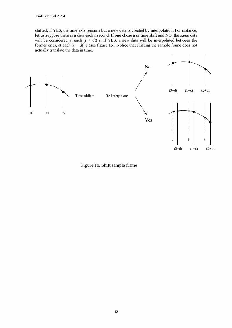
In addition, one can change the sample frame using <File|Shift sample frame>, and

specifying the time shift in seconds. The sample frame is the moment in time where each

measurement is taken. The software also creates a second dialog box, prompting for re-

interpolate data points or not. If the user answers NO, the sample frame (time axis) is just

Tsoft Manual 2.2.4

12

shifted; if YES, the time axis remains but a new data is created by interpolation. For instance,

let us suppose there is a data each t second. If one chose a dt time shift and NO, the same data

will be considered at each (t + dt) s. If YES, a new data will be interpolated between the

former ones, at each (t + dt) s (see figure 1b). Notice that shifting the sample frame does not

actually translate the data in time.

t0 t1 t2

t0+dt t1+dt t2+dt

t

0

t

1

t

2

Yes

No

Time shift =

dt

Re-interpolate

?

t0+dt t1+dt t2+dt

Figure 1b. Shift sample frame

Tsoft Manual 2.2.4

13

4. Synthetic tides

4.1.1 Management of the Location database

TSoft is equipped with a location database, a manager for locations and synthetic tides, i.e.

series of tidal parameters under the form of a wave table (up to now, only vertical tides are

supported). For each location, multiple synthetic tides can be stored. In this way, one can

store tides that include the phase lags of the instruments (for calculation of residuals during

the data correction), and “true” tides that can be used for analyses. The information is

maintained on the hard disk in a text file called “/TSOFT/LOCAT.TSD” (the format of file is

explained in Appendix 2). The location database can be opened using the menu option

<Tide|Synthetic tides|Open location database>, which creates a new window.

Figure 2. The location database window.

NB: Tidal parameter sets supplied with tsoft are basically

illustrative, though generally realistic. Users needing reference

tidal parameter sets for a station should apply to the persons in

charge of the station or take contact with ICET.

The left part of location database window shows a list containing the names of all locations

that are currently in the database.

The description of a particular location can be shown by selecting the name and using the

menu option <Location|Edit location>, or by double-clicking on the location name. A dialog

box is shown, prompting for the location's name, a description string, longitude and latitude

(both in decimal notation, positive towards East), and height above sea level. The menu

option <Location|Add location> can be used to create a new location and specify the

parameters (for Solid Earth or Ocean Loading). On the other hand, <Location|Delete>

removes the currently selected location. When the changes of the database are completed, it

can be saved to disk using <File|Save>.

The right hand part of the window shows the synthetic tides that are known for the currently

selected location (a location is selected by clicking with the mouse on it's name). In order to

Tsoft Manual 2.2.4

14

edit the parameters of a particular tide, click with the mouse on it's name and call the menu

option <Theotide|Edit parameters>.

This pops up a “tidal parameters set” dialog box, prompting for the name of the synthetic tide

(which should contain NO spaces inside), and the amplitudes and phases of the different wave

groups. The wave table should have the following formats:

A) Solid Earth Tide

1. Each wave group is written on a separate line (a new line in the edit box is created by

typing CTRL+ENTER, not ENTER!). This table can be cut from the PRETERNA

settings file, and pasted immediately in this field;

2. Each line contains the minimum and maximum frequency inside the group (in cycles

per day), the amplitude factor (), the phase shift (actually phase lead, in degrees), and

the name of the wave group.

IMPORTANT: for other tidal signals such as tilt tides, strains, etc. see H.-G. Wenzel’s

ETERNA package (http://www.eas.slu.edu/GGP/ETERNA/ ).

B) Ocean Loading

1. This file must absolutely contain the 11 waves M2, …, Ssa (see Example 2);

alternatively the names may be sM2, …, sSsa or fM2, …, fSsa (i.e. starting with s, f

or nothing);

2. Each wave group is written on a separate line (a new line in the edit box is created by

typing CTRL+ENTER, not ENTER!);

3. Each line contains the wave group name, “:”, the amplitude factor (m/s²) and the

phase shift (actually phase lead, in degrees) (see Example 2).

Tsoft does not calculate the Ocean Loading parameter sets. This can be done on H.-G.

Scherneck’s free ocean loading provider (http://www.oso.chalmers.se/~loading/), ask for

“gravity in µm/s²” and “BLQ format”. Also available, a “BLQ to Tsoft” converter: “olgt.pl”

(http://froste.oso.chalmers.se/hgs/4HW/olgt.pl, thank you, Hans-Georg!): this not only sorts

the waves in the format shown on Example 2, but also modifies the phases (local in Tsoft’s

convention, as for the Microg-LaCoste g software), referenced to Greenwich in BLQ’s

conventions. After running olgt ignore the two header lines when copying the coefficients in

the Tsoft window.

The remainder of the dialog box is currently of no use.

EXAMPLE 1: Solid Earth Tide: a wave group table of observed tidal parameters,

determined by performing a tidal analysis (using the ETERNA package) on data from a

gravimeter measuring at the station Membach (Belgium):

0.000000 0.002427 1.00000 0.0000 long

0.002428 0.720000 1.16000 0.0000 Mf

0.721500 0.906315 1.14648 -0.1916 Q1

0.921941 0.940487 1.14951 0.1094 O1

0.958085 0.974188 1.15837 0.2211 NO1

0.989049 0.998028 1.15012 0.2550 P1

0.999853 1.000147 1.19961 4.0402 S1

1.001825 1.003651 1.13746 0.2797 K1

1.005329 1.005623 1.26133 1.3710 PSI1

1.007595 1.011099 1.17383 0.4868 PHI1

1.013689 1.044800 1.16130 0.1066 J1

1.064841 1.216397 1.15588 0.1141 OO1

1.719381 1.872142 1.16068 3.4519 2N2

1.888387 1.906462 1.17587 3.0924 N2

1.923766 1.942754 1.18796 2.4558 M2

http://www.eas.slu.edu/GGP/ETERNA/

http://www.oso.chalmers.se/~loading/

http://froste.oso.chalmers.se/hgs/4HW/olgt.pl

Tsoft Manual 2.2.4

15

1.958233 1.976926 1.19241 1.0740 L2

1.991787 2.002885 1.19292 0.7627 S2

2.003032 2.182843 1.19405 1.0236 K2

2.753244 3.081253 1.05928 0.4615 M3

3.791964 4.000000 0.29360 36.4534 M4

EXAMPLE 2: Ocean loading parameters computed for the Membach Station using the

Schwiderski model (this computation is not possible using Tsoft).

sM2 : 1.7767e-008 57.4910

sS2 : 5.7559e-009 29.2300

sK1 : 2.0613e-009 61.2080

sO1 : 1.4128e-009 163.7230

sN2 : 3.6181e-009 73.3350

sP1 : 6.5538e-010 74.4490

sK2 : 1.4458e-009 27.7160

sQ1 : 3.8082e-010 -128.0930

sMf : 1.4428e-009 4.5510

sMm : 4.4868e-010 -5.7530

sSsa : 1.0951e-010 11.7800

A new tidal parameter set can be added to the list using <Theotide|Add new> (make sure the

right location is selected). <Theotide|Compute tidal parameters> allows the user to

compute directly a latitude dependent tidal parameter set using an inelastic non-hydrostatic

Earth model (from Dehant, Defraigne, Wahr, J. Geophys. Res. 104 B1, 1035-1058, 1999), see

Example 3. An existing tide is removed with <Theotide|Delete>. When the changes of the

database are completed, it can be saved to disk using <File|Save>.

***************************************************************************

!!!!IMPORTANT REMARK !!!!

The loading calculation by Tsoft will result in the correction, not the effect.

On the other hand the prediction of the solid Earth tides using the WDD parameter set

provided by Tsoft directly will result in the effect. Therefore both must be treated with

different sign in order to reduce a gravity time series correctly.

Alternatively you may run “olg.pl –r”, which reverses the sign of the amplitudes of the

loading parameters, or equivalently, “olg.pl –R”, which switch the phases by 180°.

***************************************************************************

EXAMPLE 3: Solid Earth Tide: a wave group table obtained from a theoretical Earth model

(Wahr Dehant Defraigne 1999 using <Theotide|Compute tidal parameters> (for a station

located at 50.6092N, 6.0067E). This wave group can be used to compute a synthetic tide

everywhere in the world, when no experimentally determined parameters are available. Note

that the ocean loading effect is not taken into account.

0.000000 0.002427 1.00000 0.0000 long

0.002428 0.249951 1.15787 0.0000 Mf

0.721500 0.906315 1.15432 0.0000 Q1

0.921941 0.940487 1.15430 0.0000 O1

0.958085 0.998028 1.14908 0.0000 P1

0.999853 1.000147 1.13448 0.0000 K1

1.005329 1.005623 1.27258 0.0000 PSI1

1.007595 1.011099 1.17072 0.0000 PHI1

1.013689 1.216397 1.15636 0.0000 OO1

Tsoft Manual 2.2.4

16

1.719381 2.182843 1.16200 0.0000 All2

2.753244 3.381478 1.07360 0.0000 M3

3.381379 4.347615 1.03900 0.0000 M4

4.1.2 Calculation of a synthetic tide

When a file is loaded into TSoft, the Location database can be used to create a new channel,

containing the synthetic tide. To this end, select the right location name and the right synthetic

tide name, and call the menu option <Theotide|Calculate>. A new channel is created,

containing the synthetic tide for the time period of the file, at the same sample rate, using the

1200 waves Tamura potential is “Solid Earth Tide” is selected. If “Ocean Loading” is

selected, Tsoft computes the ocean loading gravity effect due to the separate tidal primary

component. The location field of the new channel is taken from the selected location, the

instrument field is “Theory”, the measurement field is equal to the tide name, and the units are

“nm/s^2”.

Note that the tidal signal is computed relative to UTC (Universal Time Coordinated).

4.1.3 Calculation of the polar motion effect on gravity

Using <Theotide|Calculate polar motion effect>, the users can calculate the effect on the

polar motion on gravity, as a function of the station coordinates. A synthetic tide must be

selected in the data base (even if its content does not have any influence on the polar motion

effect!).

This tool calculates the changes in centrifugal acceleration due to variation of the distance of

the Earth’s axis from the gravity station. Delta=1.164. Pole coordinates are available on

ftp://hpiers.obspm.fr/iers/eop/eopc04/. The EOPC04.YY files must be installed in the

directory \Tsoft\Database\EOPC. The Formula is specified in the IAGBN Absolute

Observations Data Processing Standards (1992):

92 10*)sincos(cossin2164.1 ypxpag [nm/s²]

( = longitude, = latitude (rad))

4.1.4 Fit tidal model

This performs a rough tidal analysis on the selected channel (for an accurate analysis, specific

tools like ETERNA should be used). The wave groups are those shown in the above Example

1 (without wave M4). The Location name must be the same as in the Location Data Base,

because the geographical coordinates are needed. One must change the Location name (using

<Edit|Rename channel>) or adapt the Location Data Base so that both names correspond.

Otherwise the following error message appears: “Location “name” is not present in data

base”.

4.1.5 Detide

This roughly removes the tide from the selected channel just by fitting a very simplified tidal

model that includes the following main waves: Mm, Mf, MTM, Q1, O1, NO1, P1, K1, J1, OO1,

2, N2, 2, M2, L2, S2, K2.

ftp://hpiers.obspm.fr/iers/eop/eopc04/

Tsoft Manual 2.2.4

17

5. Correction of the raw data

5.1 Introduction

Raw data, coming immediately from an instrument, often contain undesired artifacts which

can corrupt the analyses. This holds in particular for the case of a gravity meter, where the

artifacts (usually) can be classified in four groups:

Spikes. In such an event, the signal deviates considerably from the expected value during a

very short period in time (usually one or a few measurement points). These spikes can be

due to instrumentation problems. It is clear that the presence such events degrades the

quality of each analysis done on the signal.

Earthquakes. An (even very weak) earthquake can cause very severe deviations of the

signal, during periods up to a few hours. If the goal of the analysis is not the earthquake

itself (but e.g. the earth tides), it should be removed from the data as well.

Steps. It often occurs that the signal of a gravity meter suddenly changes without any

(geo)physical reason (but e.g. due to instrumentation problems), and remains stable at the

new value afterwards. Clearly, the accumulation of such steps can strongly influence the

long-term drift behaviour.

Gaps. Due to instrument failure, the time series of a registration may be interrupted at

certain moments. Those interruptions may vary from one data point to several weeks.

For spikes and earthquakes, there are two possible ways of correction: (1) removing the bad

data points and leaving a gap, or (2) replacing the bad data points by some interpolation. The

first method has the advantage that no artificial data is introduced, but is has a number of

disadvantages. Firstly, the absence of even one single raw data point may cause the absence

of more than one day of data in the final (1 hour sample interval) data set, due to the anti-

aliasing filter that must be applied when decimating the data. And secondly, many analysis

methods (e.g. FFT) suffer from the presence of gaps in the time series. Therefore, it is

preferable (at least for short perturbations) to interpolate the data. Perhaps steps are the most

difficult events to deal with, because the introduction of a step influences the values of all

future data. Gaps can be interpolated or left in the time series, depending on their length and

the type of analysis to be performed with the data.

It is also important to notice that TSoft can correct any kind of measurement, and not only

gravity signals (e.g. air pressure or other environmental data).

5.2 Calculation of the residuals

In TSoft, the correction of the data is, whenever possible, done on the level of the residuals.

However, there are circumstances where one can not calculate residuals (e.g. when no tidal

information is present, or when correcting other channels, such as pressure or environmental

parameters).

A powerful feature of TSoft is actually that it can, at any moment, undo (and modify)

corrections that have been performed earlier on a particular channel. However, to this end,

two copies of this channel should be present. Both channels should have exactly the same

information fields, except that the measurement field of the first channel should end with

“#raw”, while the second channel should end with “#corr”. The first channel should be kept

unchanged, while the corrections (interpolations, etc.) are performed on the second one. Of

course, it is perfectly possible to correct data with only one single channel, but it will be

impossible to undo interpolations and steps later on.

Tsoft Manual 2.2.4

18

In order to be able to calculate residuals, a channel containing the synthetic tide of the

location should be present. This can be calculated using other software, or using TSoft for

vertical gravity (see section 0). Firstly, a new channel, which will be filled with the residuals,

should be created and the information fields should be filled in properly. Secondly, the

residuals can be calculated by highlighting this channel and evaluating a mathematical

expression containing the difference between the observed tide and the synthetic tide (if

present, the pressure can be corrected as well).

EXAMPLE: suppose a raw file from a location “Site” and an instrument “Gravimeter”

contains two channels: (1) the gravity and (2) the pressure. If this file is loaded, the

channel window look like:

Site Gravimeter

1 Vgrav [nm/s^2]

2 Pressure [hPa]

Step 1: Add synthetic tide. Open the Location database with <Tide|Synthetic

tides|Location database>, select the location “Site” and a corresponding tide (assume it's

name is “Vgrav”), and call the menu option <Theotide|Calculate>. This results in the

following set of channels:

Site Gravimeter

1 Vgrav [nm/s^2]

2 Pressure [hPa]

Theory

3 Vgrav [nm/s^2]

Step 2: Calculate the residuals. Call <Edit|Add channel>, highlight the new channel

(which has number 4), call <Edit|Rename channel> and fill in the parameters “Site”,

“Gravimeter”, “Vgrav resid #raw”, “nm/s^2”. Then fill this channel by calling

<Calculate|Evaluate expression> and enter “[1]-[3]+3.2*[2]” (assuming that

3.2 is the chosen air pressure admittance factor).

Create now the corrected residuals channel: call <Edit|Duplicate channel>, highlight the

new channel, call <Edit|Rename channel> and type “Vgrav resid #corr” in the

measurement field. The channel window now looks like:

Site Gravimeter

1 Vgrav [nm/s^2]

2 Pressure [hPa]

4 Vgrav resid #raw [nm/s^2]

5 Vgrav resid #corr [nm/s^2]

Theory

3 Vgrav [nm/s^2]

5.3 Correction of the artifacts

5.3.1 The concept and usage of correctors

TSoft uses the concept of correctors for the removal of artifacts on a data channel. A corrector

can be one of the following objects:

A linear interpolation. This corrector changes the data points during a certain time interval

into a linear function.

Tsoft Manual 2.2.4

19

A cubic interpolation, which changes the data into a third degree polynomial

A step, which adds a constant value to all data points after a given moment in time

A gap. This corrector removes all data points during a certain time period.

In the software, a corrector is represented graphically on the curve using a set of node points

and connecting lines. The shape and properties of each corrector can be changed by the user

by clicking the left mouse button on one of the node points, and dragging it to a new position

while holding down the mouse button.

Most of the functions in TSoft act only on the selected correctors. A single corrector can be

selected by clicking the left mouse on one of it's nodes, while a group of correctors can be

selected by drawing a rectangle around them by pressing and holding down the left mouse

button (the correctors outside the rectangle become unselected). Selected correctors appear

with blue node points, unselected ones have gray nodes.

Figure 3. Graphical representation of the different correctors in unapplied state. Left: linear and cubic

interpolations; middle: step; right: gap. The node points are drawn as black circles.

Figure 4. Same correctors, but this time in applied state (the cubic interpolation has been omitted).

Each corrector that is defined on a curve can have two states:

1. Unapplied state. In this case, the action of the corrector is not yet applied on the data (i.e.

the data points still have their raw value). At this moment, the user can still change it's

shape.

2. Applied state. In this case, the corrector is actually applied on the data, and its shape

cannot be changed.

The user can change the state of the selected corrector(s) using the menu commands

<Correctors|Apply selected> and <Correctors|Unapply selected>. Moreover, the selected

corrector(s) can be entirely removed from the channel by using <Correctors|Delete

selected>.

The most important advantage of the concept of correctors is that it provides a very flexible

and interactive way of processing the data. A typical processing session consists of the

following steps:

1. The computer automatically searches all irregular events on the channel, and calculates a

corrector for each one (all correctors are in an unapplied state).

Tsoft Manual 2.2.4

20

2. The proposed correctors are drawn on the curve, and the user can inspect them visually.

The user can ask the computer to apply and unapply a set correctors in order to see the

effect on the data.

3. If necessary, the user can change the shape of certain correctors manually. In addition,

he/she can also introduce additional ones, ore delete existing ones.

4. Finally, all remaining correctors are applied on the data.

This approach has the advantage that it combined (fast and objective) automatic detection

with a possibility for an interactive manual intervention. The latter possibility is very

important, because there will always be (strong) perturbations in complex situations that are

not treated correctly by automatic algorithms.

5.3.2 Manual creation of correctors

In order to introduce new correctors manually, put the red curve cursor at the place of the

perturbation by clicking there with the left mouse button. The menu options

<Correctors|New interpolation (linear)>, <Correctors|New interpolation (cubic)>,

<Correctors|New step> and <Correctors|New gap> can be used to create one of the four

types of correctors.

5.3.3 Automatic creation of correctors

TSoft contains algorithms that detect automatically spikes, earthquakes, step and gaps on the

signal, and that calculate a corrector for each one.

The menu option <Correctors|Auto detect spikes> is used for the detection of spikes and

earthquakes on the highlighted channel, using an algorithm which is described in section 0. A

dialog box appears, prompting for the different parameters. The first parameter is the

minimum deviation a spike should have in order to be detected (the other ones are described

in the Appendix).

<Correctors|Auto detect gaps> is used for the detection of gaps in the highlighted channel,

using an algorithm described in section 0. The dialog box prompts for the type of

interpolation (straight connection of last and first points, linear interpolation using a fit and

third degree polynomial interpolation, or add 0), and some other parameters described in the

appendix.

Finally, <Correctors|Auto detect steps> detects steps in the highlighted channel (the

algorithm is described in section 0). In the dialog box, the minimum step value is prompted,

as well as some other parameters that are related to the search algorithm.

Due to the nature of the detection algorithms, the best approach is first to detect and correct

spikes, then to detect and correct gaps, and finally to detect and correct steps (although this

ordering is not necessary).

EXAMPLE: continuing with the previous example, the following steps can be used to

correct the data:

5. Highlight channel 5 (Vgrav resid #corr), and detect spikes with <Correctors|Auto

detect spikes>. Inspect the proposed correctors and change them if necessary. Apply the

correctors using <Correctors|Select all> and <Correctors|Apply selected>.

6. Detect gaps with <Correctors|Auto detect gaps> and apply the correctors using

<Correctors|Apply selected>.

7. Detect steps with <Correctors|Auto detect steps>. Inspect the proposed correctors

and change them if necessary. Apply the steps using <Correctors|Select all> and

<Correctors|Apply selected>.

Tsoft Manual 2.2.4

21

5.3.4 Storage of step information

A complication of steps occurring on a data channel is that their corrections influence all the

future data points of that channel. In order to simplify the addition of the accumulated step

values on a new file, TSoft offers the opportunity to store the steps (time and value) in the

instrument database (see also section 0). With <Correctors|Copy applied steps to

database>, the applied steps on the highlighted channel for the time period of the file are

copied to the database. Later on, when a new file is treated, the accumulated value of all

previous steps can be calculated highlighting the appropriate channel and using

<Correctors|Calculate accumulated step value>.

5.4 Calculation of the corrected tide

When the residuals is corrected properly, it is possible to restore the corrected tide by adding

the corrected residuals to the synthetic tide (if necessary, the pressure should be incorporated

as well). Again, this can be done using the <Calculate|Evaluate expression> menu option.

This time however, the signs in the formula should be changed: if for example the formula for

the calculation of the residuals is:

residuals = tide - synth.tide + 3.2 * pressure,

then the inverse formula for restoring the corrected tide is:

tide= synth. tide + residuals - 3.2 * pressure.

EXAMPLE: continuing with the previous example, the corrected tide can be calculated in

the following way:

8. Highlight channel 1 (Vgrav), call the menu option <Calculate|Evaluate expression>

and fill in the expression “[3]+[5]-3.2*[2]”.

Tsoft Manual 2.2.4

22

6. The instrument database

6.1.1 Introduction

TSoft includes a database which greatly simplifies the organization of the different files

containing registrations from various instruments, as well as some other important parameters

(such as calibration information). Any user is free to use this database or not; most functions

of TSoft work fine even if this database is not used.

Physically, the database information is maintained in a text file “\TSOFT\DBASE.TSD”,

using a file format described in section 0. It is possible to merge the information coming from

different files by simply linking them together in a text editor.

Up to now, a TSoft database may contain four different types of information:

Installations. For each installation of a instrument, a field can be added in the database,

containing the data, the name of the instrument and the name of the location. This event is

only of interest for portable instruments.

Calibrations. Each time a calibration of a particular data channel has been performed, a

field can be added, containing the name of the instrument and measurement, the date and

the calibration value. This information can be particularly useful for instruments that have

a sensitivity changing with time (e.g. some types of spring gravity meters).

Steps. The steps that occurred on each data channel can be stored, by specifying the

instrument and measurement, the date, and the step value (see also section 0).

Time shift corrections. Deviations of the data acquisition clock from the true time can be

specified in the database. This information can be used to compensate such deviations.

File information. For each instrument, and for each measurement, a list of files that

contain information concerning that particular data channel can be maintained.

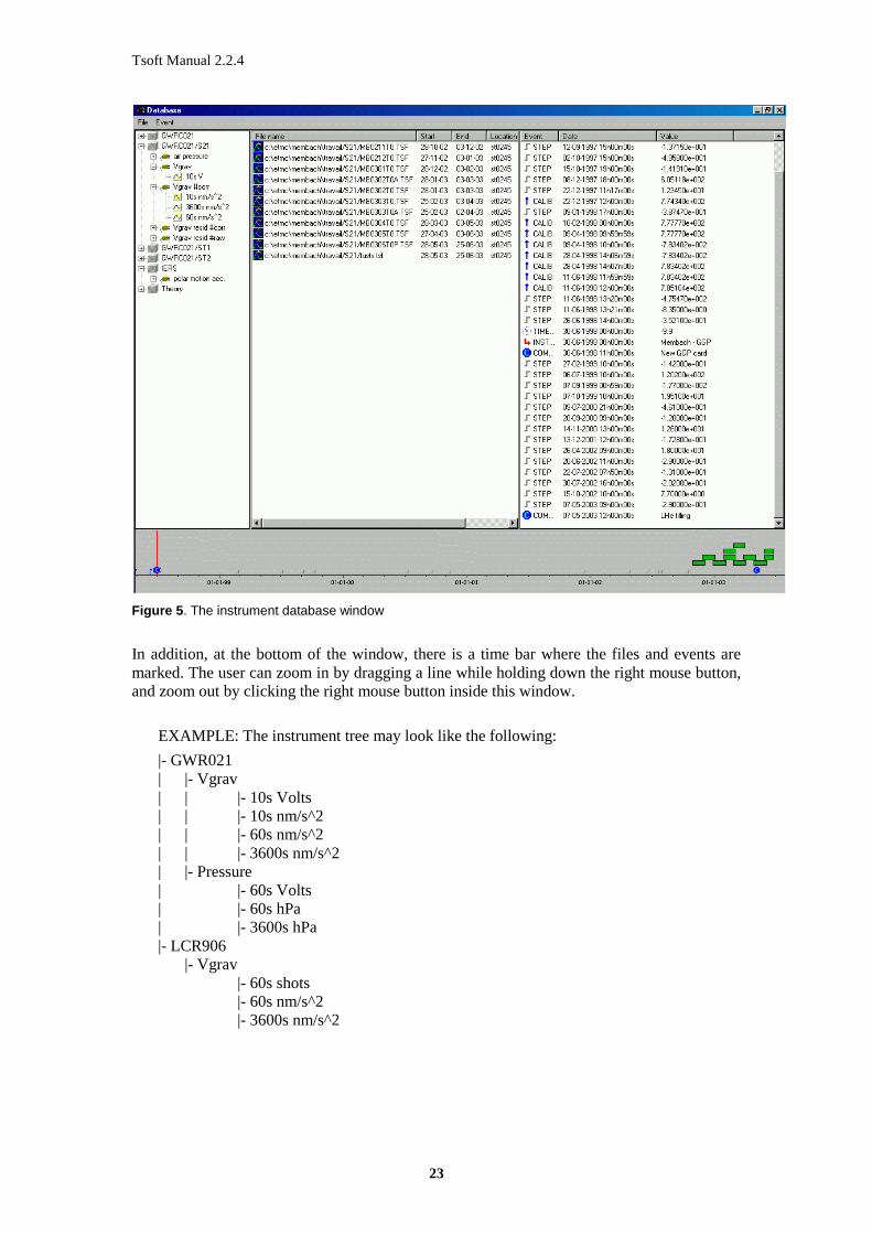
6.1.2 Presentation of the database

The instrument database can be called using the menu option <File|Open database>. A new

window (the database window) appears, divided in three parts. From left to right, there are:

The instrument tree. This window contains an overview of the instruments and their

measurements, arranged in a tree structure. At the lowest level, the instruments are listed.

For each instrument, the different measurements are displayed at a higher level. Finally,

for each measurement, the different data variants are listed at the highest level (a data

variant is a combination of a sample rate and a physical unit). At the highest level of the

tree, the instrument, measurement and data variant are determined in a unique way. The

various branches in the tree can be collapsed and expanded by clicking inside the small

boxes containing + and - signs, just as in the Windows95 Explorer. A particular

instrument, channel or data variant can be selected using the left mouse button.

The instrument file list. When a data variant is selected, this window shows a list of files

that are known to have a channel containing this information. The file name, start and end

date of the file and the location are shown. One or more files may be selected by clicking

on the file name. The selected file(s) may be loaded using <File|Open selected file(s)>.

The instrument event list. When a particular measurement is selected, this window

displays a list of events (calibrations, steps, etc.) that are currently defined for that

measurement. For each event, the nature, the date and time of occurrence, and the

corresponding value is shown. The user can select an event by clicking on the first field.

Tsoft Manual 2.2.4

24

6.1.3 Adding and changing information

If a data file is loaded in TSoft, its channels may be added to the database using the

<File|Add current file to index> menu option. Moreover, one can add the contents of all the

TSF files in a complete directory structure by using <File|scan file structure>, and

specifying the directory (with subdirectories) that should be scanned.

A new installation event can be added to the database by selecting the appropriate instrument

in the instrument tree, and calling <Event|New installation>. A dialog box prompts for the

date and time, and the new location.

In order to add a new calibration, select the appropriate measurement in the instrument tree

and call <Event|New calibration>. A dialog box prompts for various parameters:

The date and time of the event.

The calibration value a

The error on the calibration value a (for information only)

Optionally, a function f(x) expressing the nonlinearity of the calibration. If this field is

empty, it is supposed that f(x)=x.

Units_from: the physical units of the uncalibrated data (e.g. Volts)

Units_to: the physical units of the calibrated data (e.g. nm/s^2)

The calibrated values are calculated using the following expression:

Calib.val. = a . f(Uncalib.val.),

so that a is expressed in units_to / units_from (e.g. nm/s^2 / Volts).

A new step can be added by selecting the appropriate measurement, calling <Event|New

step> and filling in the date, the step value and the physical units of this step value. See also

section 0 concerning automatic addition of steps.

A new time shift correction can be entered by selecting the appropriate instrument and

measurement, and calling <EventAdd time shift>. A dialog box appears, prompting for the

time and date of measurement and the time deviation value (in seconds), defined as

deviation= true time - data acquisition time.

A selected existing event can be re-edited using <Event|Edit event> (the date and time can

not be changed anymore), or deleted using <Event|Delete event>.

6.1.4 Calibrating a channel using the instrument database

When a file is loaded containing an uncalibrated channel, it can be calibrated by highlighting

it and calling <Tides|Calibration|Calibrate channel>. A dialog pops up, prompting for the

desired units of the calibrated channel. During the calibration process, the following

procedure is followed:

1. The instrument database is scanned for calibration events that concern the right instrument

and measurement.

2. From this set of calibrations, those are kept that have the same units_from as the

uncalibrated channel, and the same units_to as specified in the dialog box. (If none are

found, the procedure stops).

3. For each data point, two calibration functions are applied: the last one before the point and

the first one after the point. Both values are interpolated in a linear way. If only one

calibration is applicable, one single calibration function is used.

4. The results are stored in a new channel.

Of course, if the calibration factor of an instrument does not change significantly in time,

there is no special need to use this feature for calibration. The evaluation of a mathematical

expression using <Calculate|Evaluate expression> may do this job very well in this case.

Tsoft Manual 2.2.4

25

6.1.5 Compensation of time shifts

Each time that the clock of an acquisition system is checked against an absolute time

reference, a new time shift event can be entered into the database, specifying the moment of

control and the deviation. TSoft can use this information in order to compensate the

deviations, and bring the data values back to the correct time frame. To this end, the different

time shifts are interpolated linearly and applied to the data set. This calculation can be

performed by highlighting the appropriate channel, and calling the menu option

<TidesCalibrationCorrect time shift> from the main window. A new channel is created,

containing the corrected data points.

When the clock of the acquisition system has been changed (e.g. in order to bring it back to

the correct time), two separate time events should be entered: a one just before the change,

containing the old shift, and a second one just after the change, containing the new time

deviation (usually zero).

Tsoft Manual 2.2.4

26

7. Analysis of the data

7.1 Introduction

TSoft can be used to apply a variety of different analysis tools on the data. The application of

these tools is completely interactive, and the results are displayed in a graphical way. In most

of the cases, the calculations are only performed on the active part of the data (see section 0

concerning active and inactive data).

In addition, some of the analysis tools require a set of selected channels. A channel can be

selected or unselected by clicking with the left mouse button inside the right hand side

rectangle that is drawn next to the channel names in the channel window (see also Figure 1).

For selected channels, this rectangle is drawn in red.

7.2 Filtering of the data

7.2.1 Filters applied in the frequency domain

FFT or spectral filtering is a powerful way of filtering a particular frequency range from a

data channel. The algorithm includes the following steps:

1. The FFT transform of the signal is calculated

2. This transform is multiplied by a given filter response function R(f) in frequency domain

3. The resulting transform is transformed back into time domain.

TSoft offers three types of filters: low-pass, high-pass and band-pass. Each type has two

parameters; the cut-off frequency or central frequency f0, and the band width fw (see also

Figure 6).

For 𝑓 < 𝑓0 − 𝑓𝑤 (low-pass) or 𝑓 > 𝑓0 + 𝑓𝑤 (high-pass), the transfer function = 1. The

transition band being given by (for 𝑓0 − 𝑓𝑤 ≤ 𝑓 ≤ 𝑓0 + 𝑓𝑤):

0.5 + 0.75 ∗𝑓 − 𝑓0

𝑓𝑤− 0.25 ∗ (

𝑓 − 𝑓0

𝑓𝑤)

3

While for the band-pass filter, it becomes:

1 − 2 (𝑓 − 𝑓0

𝑓𝑤)

2

+ (𝑓 − 𝑓0

𝑓𝑤)

4

Figure 6. Filter response functions of the low-pass (left), high-pass (middle) and band-pass (right) FFT

filters.

Tsoft Manual 2.2.4

27

To apply a filter on a data channel, highlight the appropriate channel and call <Filters|FFT

filtering>, choose the correct filter type and fill in the cut-off frequency and band width (both

in Hz or, if selected, cycles per day). A new channel is created, containing the filtered signal.

IMPORTANT NOTE:

When transformed to time domain, one can easily see that these filters would have an

infinite length in time (this is in contrast to e.g. the LSQ filtering, which has a limited

number of points, specified by the user). In other words, each point of the filtered signal

depends in principle on all points of the data channel, from minus infinity to plus infinity.

As a consequence of this, the results of this filter are (very slightly) influenced by the

limitations in time of the series and by the presence of gaps. Therefore, these filters

should not be used as anti-aliasing filters in the routine reduction of the data, but rather as

a powerful tool for the analysis and the investigation of the data.

7.2.2 Filters applied in the time domain

Three types of low-pass time domain filters are present in TSoft (for more details about the

mathematical principles, see the literature):

Least squares (LSQ) filtering. Highlight the channel and call <Filters|Least squares

filtering> for high or low-pass filtering. The dialog box prompts for the cut-off frequency

and the number of points of the filter. Call <Filters|Band pass least squares filtering> for

band pass filtering.

Polynomial (Savitsky-Golay) filtering. Highlight the appropriate channel and then call

<Filters|Polynomial filtering>. The dialog box prompts for the number of points of the

filter and the degree of the polynomial. Optionally, “smooth edges” causes the weight of

the polynomial fit to decrease linearly towards the edges, a modification which improves

the properties of the filter.

Butterworth filtering (2 poles): Highlight the channel and call <Filters|Butterworth

filtering> for high or low-pass filtering. The dialog box prompts for the cut-off frequency.

Because of its very good frequency response properties, the LSQ filtering is the best choice as

an anti-aliasing filter for the reduction of the sample rate of a signal. For example, before the

reduction of a 1 min sample interval data channel to a 1 hour sample interval, a LSQ filter

with cut-off frequency of 12 cpd and window size of 480 points can be applied. This filter has

a total length of 16 hours, and the frequency response curve deviates in the tidal frequency

band less than 0.05% from unity.

TIP: How to see the filters transfer functions:

1) Create a channel with a step function (with the sgn function using <Calculate|Evaluate

expression> (e.g. : 1-sgn(a-t), where a is the step position (in days) );

2) Apply the filter;

3) Position the curve cursor (red cross) at the beginning of the filtered step and use the

<Calculate|Transfer function> command. Two windows appear: “Transfer function

(normalised amplitude)” and “Transfer function (group delay)”.

Another possibility to see the amplitude response is to apply the filter on a white noise. This

noise is obtained applying <Calculate|Plug-Ins|Add Gaussian White Noise> on a constant

channel (e.g. created by just entering the number 0 in <Calculate|Evaluate expression>).

Tsoft Manual 2.2.4

28

7.3 Multilinear least squares fits

7.3.1 Straightforward fits.

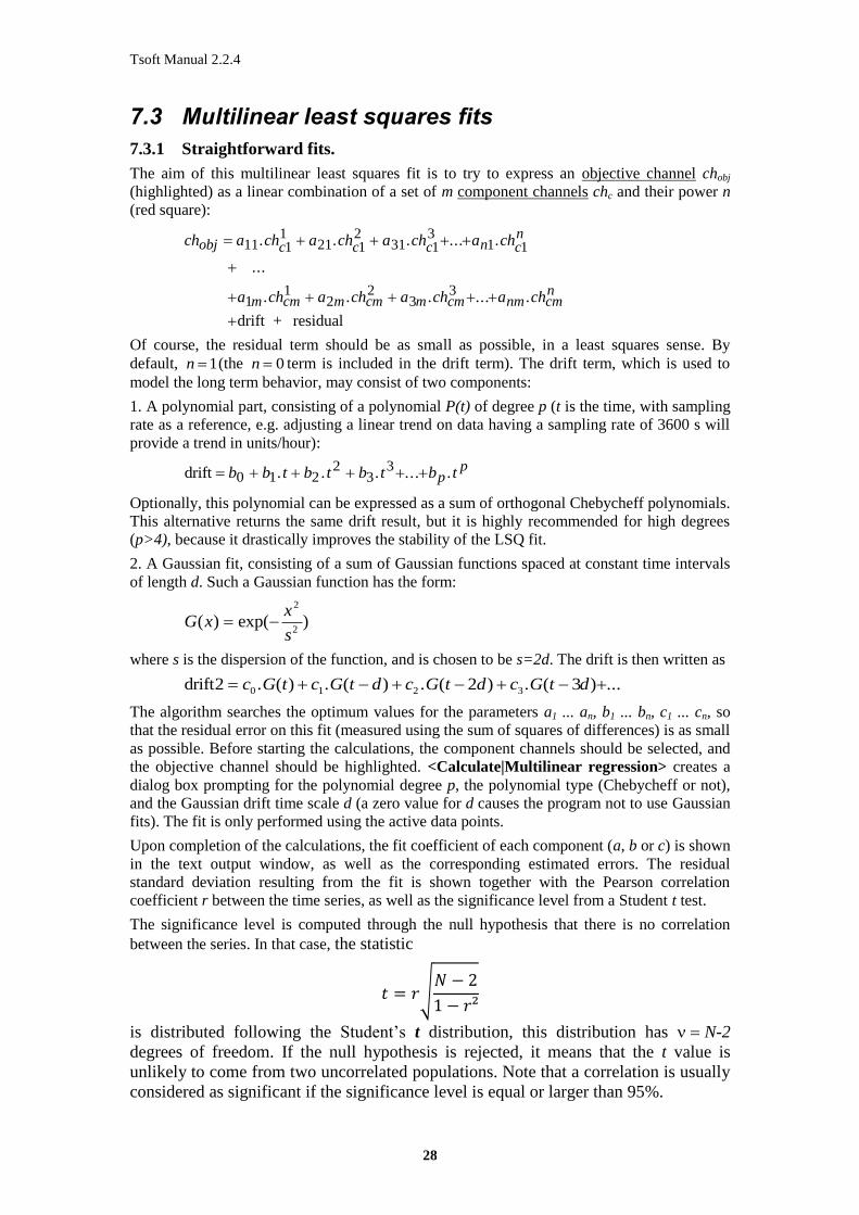
The aim of this multilinear least squares fit is to try to express an objective channel chobj

(highlighted) as a linear combination of a set of m component channels chc and their power n

(red square):

ch a ch a ch a ch a ch

a ch a ch a ch a ch

obj c c c n cn

m cm m cm m cm nm cmn

11 11

21 12

31 13

1 1

11

22

33

. . . ... .

...

. . . ... .

drift + residual

Of course, the residual term should be as small as possible, in a least squares sense. By

default, n 1(the n 0 term is included in the drift term). The drift term, which is used to

model the long term behavior, may consist of two components:

1. A polynomial part, consisting of a polynomial P(t) of degree p (t is the time, with sampling

rate as a reference, e.g. adjusting a linear trend on data having a sampling rate of 3600 s will

provide a trend in units/hour):

drift b b t b t b t b tpp

0 1 22

33. . . ... .

Optionally, this polynomial can be expressed as a sum of orthogonal Chebycheff polynomials.

This alternative returns the same drift result, but it is highly recommended for high degrees

(p>4), because it drastically improves the stability of the LSQ fit.

2. A Gaussian fit, consisting of a sum of Gaussian functions spaced at constant time intervals

of length d. Such a Gaussian function has the form:

G xx

s( ) exp( )

2

2

where s is the dispersion of the function, and is chosen to be s=2d. The drift is then written as

drift2 2 30 1 2 3 c G t c G t d c G t d c G t d. ( ) . ( ) . ( ) . ( ) ...

The algorithm searches the optimum values for the parameters a1 ... an, b1 ... bn, c1 ... cn, so

that the residual error on this fit (measured using the sum of squares of differences) is as small

as possible. Before starting the calculations, the component channels should be selected, and

the objective channel should be highlighted. <Calculate|Multilinear regression> creates a

dialog box prompting for the polynomial degree p, the polynomial type (Chebycheff or not),

and the Gaussian drift time scale d (a zero value for d causes the program not to use Gaussian

fits). The fit is only performed using the active data points.

Upon completion of the calculations, the fit coefficient of each component (a, b or c) is shown

in the text output window, as well as the corresponding estimated errors. The residual

standard deviation resulting from the fit is shown together with the Pearson correlation

coefficient r between the time series, as well as the significance level from a Student t test.

The significance level is computed through the null hypothesis that there is no correlation

between the series. In that case, the statistic

𝑡 = 𝑟√𝑁 − 2

1 − 𝑟²

is distributed following the Student’s t distribution, this distribution has N-2

degrees of freedom. If the null hypothesis is rejected, it means that the t value is

unlikely to come from two uncorrelated populations. Note that a correlation is usually

considered as significant if the significance level is equal or larger than 95%.

Tsoft Manual 2.2.4

29

Except for white noise, the number of degrees of freedom is not the number of data

and has to be estimated using time series model. Here, is the geometrical average of

the degree of freedom of each series (von Storch, 1999), estimated using the

autocorrelation tool (see the description of Autocorrelation here after). The number

of degrees of freedom is provided in the text output window.

In addition, two new channels are created: 1. The fit to the objective channel is stored in a channel having extension “(fit)”.

2. The residuals of the fit (=objective channel minus the fit result) is stored in a channel

having extension “(resid)”.

7.3.2 Moving window multilinear least squares fits

This analysis tool is an extension of the multilinear least squares fit. Rather than performing

one single fit using all the active data points over the whole time span of the file, this module

performs a fit in a set of time windows., which have a constant length tw. Each window is

shifted over a constant time interval ts with respect to the previous (see Figure 7).

Figure 7. Schematic representation of the moving window regression.

In each window, a least squares fit is performed on the objective channel using the component

channels. In this way, it is possible to obtain a plot of the variations of the coefficients as a

function of time.

Optionally, it is possible to apply a FFT filter to all the channels (components as well as

objective) before the fit is performed. In this way, it is possible to study the behaviour in a

certain frequency band.

As for an ordinary least squares fit, the component channels should be selected, and the

objective channel should be highlighted. Use the menu option <Calculate|Moving window

regression> to create a dialog box that prompts for various parameters:

The window size tw and the window separation ts (both in data points)

The degree of the polynomial that models the drift (this parameter should be zero if the

applied filter does not include very low frequencies)

The LSQ filter type and parameters (see section 0)

Whether the obtained points should be connected with a linear interpolation or not.

Tsoft Manual 2.2.4

30

When the calculations are completed, a number of new channels are created:

1. For each component channel, a new channel is created having the same measurement field,

but with a “COEF:” inserted at the start. These channels contain the time-dependent

variation of the component coefficients. On the data points, the error bars resulting from

the fit are also indicated.

2. A channel, called “Residual error”, which contains the root-mean-square (RMS) value of

the residuals inside each window

3. A channel, called “Drift”, containing the mean value of the polynomial drift model inside

each window.

EXAMPLE: A very useful application of this tool is the monitoring of the long-term

variation of the sensitivity of an instrument, using a fit to a synthetic tide. As component

channels, one can take (1) the synthetic tide, (2) the time derivative of the synthetic tide

(in order to estimate phase shifts) and (3) the air pressure. Using the observed tide as

objective channel and a window size of a few weeks, this function allows one to obtain a

plot of the variation of sensitivity and phase (expressed in seconds).

7.3.3 Frequency-dependent multilinear least squares fits

In many cases, the regression coefficient of a component channel is actually depending on the

frequency. TSoft offers a tool to investigate this frequency dependency. The idea is to apply

to all channels a set of narrow band pass filters over a range of frequencies, and to perform

the regression on each set of resulting filtered channels. The different values of the

coefficients corresponding to different filter frequencies then reflect the dependency on the

frequency.

To use this function, select the component channels and highlight the objective channel, and

call the menu option <Calculate|Frequency dependent regression>. A dialog box appears,

prompting for a number of various parameters:

The minimum and maximum frequency of the range of filter frequencies

The frequency increment, i.e. the frequency step between two adjacent band-pass filters

The band width of each filter.

The number of points (LSQ filter only).

Upon completion of the calculation, a number of new windows are created:

1. For each component channel, a new window shows a plot of the frequency dependent

coefficient

2. A last window shows a plot of the correlation of the fit as a function of the frequency.

EXAMPLE: An interesting application of this feature is the investigation of the frequency

dependence of the admittance factor of the local air pressure. As component channels,

select the local air pressure and it's time derivative. As objective channel, highlight a

channel containing the difference between the observed tide and the synthetic tide (e.g.

calculated using <Edit|Add channel-> and <Calculate|Evaluate expression>). Call

<Calculate|Frequency dependent regression>, and e.g. fill in a frequency range from 0

cpd to 7 cpd, an increment of 0.2 cpd and a band width of 0.3 cpd. After calculation, the

frequency dependency of the admittance factor and the phase (in seconds) is shown.

Tsoft Manual 2.2.4

31

7.3.4 X-Y plots

TSoft can plot one channel as a function of the other. Highlight the channel which should be

on the X axis and call <Calculate|Create new X-Y window> in order to create a new, empty

X-Y window. Then proceed by highlighting a channel which should be on the Y axis and call

the menu option <XYgraph|Add new channel> in order to display the plot. Up to 4 Y axis

channels may be added into one window. It is possible to zoom in and out in the same way as

on a curve in the main window.

7.4 DeCAC: removing the composite cycle

DECAC is very useful to process environmental data, e.g. it allows removing easily the

annual component.

DECAC makes use of a stacking technique (Hartmann and Michelsen, 1989). This tool allows

removing the mean signal of period T. This is done by first computing the mean signal for a

given phase by averaging all the value of the time series corresponding to this phase (t = ,

T+ , 2T+ , …), then by removing it at every data point of this phase,

7.5 Calculation of spectra

7.5.1 Simple spectra

Spectra of channels are displayed in a spectrum window. A new, empty, spectrum window

can be created using the menu option <Calculate|New spectrum window>. In order to add a

new spectrum to the window, highlight the appropriate channel and call the menu option

<Spectrum|Add new channel> from the spectrum window. It is possible to add up to 4

spectra in one window, all displayed with different colours.

The software uses FFT to calculate the spectrum, padding the data with constant values up to

a power of 2, and using (multiple) Hanning (by default), Parzen or Square window functions.

The spectrum is calculated using the active points only. It is possible to select the data

windowing by clicking <Spectrum|Windowing options>.

Initially, the (horizontal) frequency scale is in Hz (1/s), but this can be changed into cycles per

day (cpd=1/86400s) using <Spectrum|Show cycles per day>. It is possible to zoom in by

pressing the right mouse button inside the black window, and drawing a rectangle around the

region of interest while holding down the mouse button. To zoom out, click with the right

mouse button without moving.

<Spectrum|Show phase> and <Spectrum|Show power spectrum> displays either the phase

spectrum, either the power spectrum.

Unit of the power spectrum is:

[unit of the channel]²/Hz

Unlike the amplitude spectrum, the power spectrum (also called Power Spectral Density PSD)

normalizes the spectrum to the frequency bandwidth used. In other words the PSD does not

depend on the length of the time series nor the sampling rate, which allows, for different

series, comparing easily the energy contained in the spectra per unit of frequency.

The PSD can be used to recover the standard deviation of the time series at a given frequency

f by using:

𝜎 = √𝑓 𝑃𝑆𝐷(𝑓)

2

Tsoft Manual 2.2.4

32

Where PSD(f) is the power spectral density level at the frequency f. For example, if the PSD

of the superconducting gravimeter is 5 (nm/s²)²/Hz at 0.01 Hz, the standard deviation is 0.16

nm/s².

<Spectrum|Sum squared amplitude inside window> writes, for all spectra, the total

spectral power of the visible part of the spectrum to the text output window.

<Spectrum|Spectral power table> calculates a table of spectral power values inside

frequency blocks with a specified width. A table is exported to a text file, and a new window

shows a graphical representation.

<File|Export> creates a 5 columns file “EXPORT.TXT” that includes automatically: 1) the

frequency (in Hz or CPD,); 2) the amplitude; 3) the phase; 4) the power spectrum; 5) the

smoothed power spectrum (moving average on 11 points). Note that it is not possible to

display this last channel on a Tsoft window.

7.5.2 Moving window spectrum calculation

In addition to the straightforward calculation of one single spectrum using all the points in the

complete time span, TSoft also allows one to calculate a series of spectra in a number of

windows in time. The windows have a constant length tw and a constant separation in time ts

(see also section 0).

This option is activated by highlighting the appropriate channel and calling

<Calculate|Moving window spectrum>. A dialog box appears, prompting for the window

length tw (= number of points to transform, should be a power of 2 due to the FFT algorithm)

and the window separation ts.

When the calculations are completed, a new window is created, showing a plot where the time

scale is on the horizontal axis, and the frequency scale is on the vertical axis. Inside the plot, a

colour scale represents the amplitude value at each point. The amplitude corresponding to

each colour can be determined using the colour lookup table which stand on the right hand

side of the window.

The frequency scale can be changed from Hz to cycles per day using <Show|Cycles per

day>. One can zoom in on the plot by pressing the right mouse button and drawing a

rectangle while holding down the mouse button. To zoom out again, click the right mouse

button without moving. In addition, it is possible to change the colours of the colour lookup

table by pressing the left mouse button on the colour bar on the right and moving the mouse

up or down while holding down the mouse button.

7.5.3 Phase graphs

A phase graph is a very simple, but sometimes very powerful tool for the investigation of the

time dependent variation of a particular frequency. First, a band pass filtering in the desired

frequency (e.g. 2 cpd) should be applied on the signal.

The phase graph algorithm rearranges all the data points into a table, in such a way that each

row represents exactly one complete period (see e.g. Figure 8). This table is then represented

in a graphical way, using a colour lookup table in order to translate the different data values

into different colours.

Tsoft Manual 2.2.4

33

Figure 8. Arrangement of the phase graph table for a 12 h period wave, for a data set sampled with 1

hour interval

The phase plot can be calculated by highlighting the appropriate (filtered!) channel, calling

<Calculate|Phase graph>, and filling in the required wave period (in hours, can be a non-

integral value). In the resulting plot, the time is on the horizontal axis, and the phase index

(0.0=0 degrees, 1.0=360 degrees) is on the vertical axis. One can zoom in and zoom out on

this graph in the usual way, using the right mouse button. The colours can be changes by

clicking with the pressing mouse button (maximum value) or the right mouse button

(minimum value) on the colour bar on the right and dragging it to a new position.

7.5.4 Nakamura

This is a seismology tool, allowing one to calculate the ground eigenfrequency, using the

Nakamura’s method. Select the horizontal channels as component channel (red) and the

vertical channel as objective channel (highlighted). Then the spectra of the three channels are

calculated, and a windows appears, giving X/Z, Y/Z and X Y

Z

² ².

7.6 Time derivatives , time integration and time shifts

The menu option <Calculate|Time derivative>/<Calculate|Time integration> calculates

the first derivative/time integration of the highlighted channel with respect to the time (in

seconds), and stores the result in a new channel. <Calculate|Time shift> shifts the

highlighted channel in time over a specified number of seconds.

7.7 Convolution

The so-called "convolution" function creates a new channel which is a linear combination of

the selected channel shifted in time. When calling this function the user is proposed to fill in

a two-column array, where columns are separated by a colon ":".

The 1st column contains entire numbers, the shift indices n(i) being the number of time

increments by which the channel is first shifted. So if the time increment of the file is 60 s,

n=+5 means the channel is shifted behind by 5 min. It actually computes ch(t + 5 * 60 s).

The 2nd column contains the coefficients values v(i) by which the channel is then multiplied.

Finally the result for one line is v(i) * ch(t + n(i) * increment) There are as many terms in the

linear combination as lines in the array.

Tsoft Manual 2.2.4

34

7.8 Correlation

The menu option <Calculate|Correlation> calculates the correlation between the highlighted

channel with respect to a component channel (in red) (using the least squares fit). Only one

component channel is allowed. This option is useful to search the time delay between two

channels. The component channel is time shifted from MIN SHIFT to MAX SHIFT and for

each step a correlation coefficient is calculated. All these coefficients are plotted in a graph.

The minimum, maximum time shifts and the step can be changed in the dialog box that is

automatically opened. By default, MIN SHIFT = -10 * time increment, MAX SHIFT = + 10 *

time increment, STEP = time increment / 10.

7.9 Autocorrelation

The menu option <Calculate|Autocorrelation> calculates the autocorrelation of the signal.

Upon completion of the calculations, the degree of freedom is shown in the text output

window. The number of degrees of freedom is the number of data divided by the decay time

(or decorrelation time) of autocorrelation (where the autocorrelation drops to 1/e = 0.3679).

This function indicates to which extend there is persistence in the data. In a white noise, all

the data are independent from each other; so that the number of degrees of freedom is the

number of data.

Note that to reduce computation time, the shift time t is incremented logarithmically.

7.10 Allan Variance

The Allan variance of a time series Xi with N items and sampling time τ is defined by:

𝜎𝐴2(𝑋, 𝜏) =

1

2𝑁∑(𝑌𝑖+1 − 𝑌𝑖)²

𝑁

𝑖=1

The Allan variance investigates the stability of the time series as a function of the averaging

time 𝜏, Yi being the mean value on that time interval.

The Allan variance can be used to investigate the noise structure: the Allan variance of a

white noise will have a slope -1 (the noise is reduced by the square root of the number of

points used for the average), a flicker noise a slope 0 (i.e. collecting more data will not

improve nor worsen your average) and a random walk noise (red noise) a slope +1 (i.e.

collecting more data will make things worse).

Note that to reduce computation time, the averaging time is incremented logarithmically.

See http://www.allanstime.com/AllanVariance/

7.11 Transfer function (FFT)

The menu option <Calculate|Transfer function (FFT)> estimates the transfer function

between one objective (y, highlighted) channel with respect to one (and only one) component

channel (x, in red). It performs a moving FFT on both the x and y channels. The FFT is

applied on j successive blocks (not overlapping), using the Hanning window. The size of the

blocks is determined in the parameter box “Block Size”. For each block j (

j Total data set length Block Size= 1,... , ), the FFT provides the real parts Rijx, Rijy and the

imaginary part Cijx and Cijy. Then Tsoft calculates:

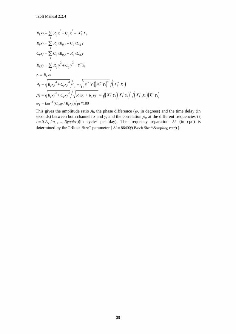
http://www.allanstime.com/AllanVariance/

Tsoft Manual 2.2.4

35

R xx R x C x X X

R xy R xR y C xC y

C xy C xR y R xC y

R yy R y C y Y Y

r R xx

A R xy C xy r X Y X Y X X

R xy C xy R xx R yy X Y X Y X X Y Y

C xy R xy pi

i ij ij ij

i

i ij ij ij ijj

i ij ij ij ijj

i ij ijj

i i

i i

i i i ii i i i i i

i i i i i i i i i i i i i

i i i

2 2

2 2

2 2

2 2

1 180

* * *

* * * *

tan ( / ) *

This gives the amplitude ratio Ai, the phase difference (in degrees) and the time delay (in

seconds) between both channels x and y, and the correlation , at the different frequencies i (

i Nyquisti i 0 2, , , ... , )(in cycles per day). The frequency separation i (in cpd) is

determined by the “Block Size” parameter ( i Block Size Sampling rate 86400 ( * ) ).

Tsoft Manual 2.2.4

36

8. Appendix I: The TSF file format

8.1 General structure

A TSF file always starts with the identifier string [TSF-file] v01.0. Future changes of

the file format will contain higher version numbers.

The file is structured using tagged blocks. Each block consists of two parts:

1. The tag, a short string delimited with square brackets []. This string is always positioned at

the very beginning of a new line.

2. The information. This part starts after the tag, and continues until a new tag or the end of

the file is reached. This part may contain return characters.

Data fields are always written in a free format. This means that different fields are separated

with at least one space, and that there is no constraint on the length of one single field.

8.2 List of possible blocks

This section contains a list of tags, together with a short description of the format and purpose

of the information parts. Tags marked in boldface should always be present in a TSF file.

Other tags may be absent. Tags marked with a * should not occur more than once in one

single TSF file.

*[TIMEFORMAT] formatstring

Determines the format of the date and time information. Currently supported is:

1) DATETIME= year month day hour min sec

2) DATETIMEFRAC= year month day hour min sec secfr

Such a block should precede any block that requires a date and time format.

[COUNTINFO] number

specifies the number of data points in the file (note that this tag is not required)

*[INCREMENT] sec

determines the time delay (in seconds) between two consecutive data points

*[CHANNELS]

channel_name_1

channel_name_2

...

channel_name _n

Determines the names of all channels in the file. Each name should be written on a separate

line, and should have the following format: location : instrument_name : data_type.

*[UNITS]

unit 1

unit 2

...

unit n

Determines the units of all channels in the file. This tag should not appear before the

[CHANNELS] tag. Each unit should be written on a separate line, and each channel should

have exactly one unit. Undetermined or unknown units should be marked with “?”

Tsoft Manual 2.2.4

37

*[UNDETVAL] number

Determines which number is used to denote undetermined or unknown values in the [DATA]

block. Note that TSoft does not take into account these values for computation.

[COMMENT] comment

Used to add comments to the file. Lines starting with a # are also considered as comment

lines, but, in contrast to [COMMENT] lines, their contents is not preserved when files are

processed or converted

[DATA]

date&time val_1 val_2 ... val_n


...


Gives the data points of the time series, each point on a separate line. The format of

data&time is specified in the [TIMEFORMAT] part. The difference in time between two data

lines should always be an integer multiple of the value specified in [INCREMENT]. In

addition, the earliest time should be equal to the one specified in [STARTTIME]. Note that it

is not required that all data points are specified in one single [DATA] block.

[LABEL] channel#

date&time

text

Assigns a comment to a particular moment in the time series on the channel with number

channel#. The date&time field gives the moment. The text field should always appear on a

separate line, and gives the contents of the comment.

[LININTERPOL] channel#

date&time1

date&time2

val1 val2

val1_0 val2_0

applied

Defines a linear interpolation corrector on channel channel#, starting at date&time1 and

ending at date&time2. The start and end values are given by val1 and val2. applied is 1 when

the corrector is applied and 0 in the other case.

[CUBINTERPOL] channel#

date&time1

date&time2

date&time3

date&time4

val1 val2 val3 val4

val1_0 val2_0 val3_0 val4_0

applied

Defines a cubic interpolation corrector on channel channel#, starting at date&time1 and

ending at date&time4. date&time2 and date&time3 are the times two intermediate points

val1, val2, val3 and val4 give the values at each point. applied is 1 when the corrector is

applied and 0 in the other case.

[GAP] channel#

date&time1

date&time2

val1 val2

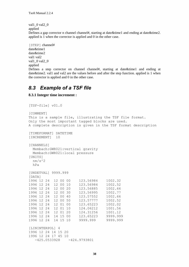
Tsoft Manual 2.2.4

38

val1_0 val2_0

applied

Defines a gap corrector n channel channel#, starting at date&time1 and ending at date&time2.

applied is 1 when the corrector is applied and 0 in the other case.

[STEP] channel#

date&time1

date&time2

val1 val2

val1_0 val2_0

applied

Defines a step corrector on channel channel#, starting at date&time1 and ending at

date&time2. val1 and val2 are the values before and after the step function. applied is 1 when

the corrector is applied and 0 in the other case.

8.3 Example of a TSF file

8.3.1 Integer time increment :

[TSF-file] v01.0

[COMMENT]

This is a sample file, illustrating the TSF file format.

Only the most important tagged blocks are used.

A complete description is given in the TSF format description

[TIMEFORMAT] DATETIME

[INCREMENT] 10

[CHANNELS]

Membach:GWR021:vertical gravity

Membach:GWR021:local pressure

[UNITS]

nm/s^2

hPa

[UNDETVAL] 9999.999

[DATA]

1996 12 24 12 00 00 123.56984 1002.32

1996 12 24 12 00 10 123.56984 1002.52

1996 12 24 12 00 20 123.56885 1002.66

1996 12 24 12 00 30 123.56995 1002.77

1996 12 24 12 00 40 123.57552 1002.66

1996 12 24 12 00 50 123.57777 1002.52

1996 12 24 12 01 00 123.65223 1002.02

1996 12 24 12 01 10 124.06212 1001.56

1996 12 24 12 01 20 124.31256 1001.12

1996 12 24 14 15 00 123.65223 9999.999

1996 12 24 14 15 10 9999.999 9999.999

[LININTERPOL] 4

1996 12 24 14 15 20

1996 12 24 17 45 10

-425.0533928 -424.9793801

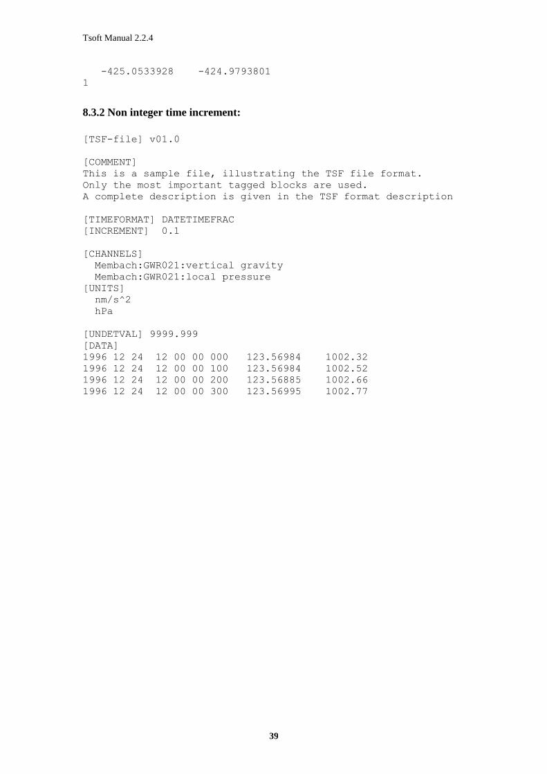
Tsoft Manual 2.2.4

39

-425.0533928 -424.9793801

1

8.3.2 Non integer time increment:

[TSF-file] v01.0

[COMMENT]

This is a sample file, illustrating the TSF file format.

Only the most important tagged blocks are used.

A complete description is given in the TSF format description

[TIMEFORMAT] DATETIMEFRAC

[INCREMENT] 0.1

[CHANNELS]

Membach:GWR021:vertical gravity

Membach:GWR021:local pressure

[UNITS]

nm/s^2

hPa

[UNDETVAL] 9999.999

[DATA]

1996 12 24 12 00 00 000 123.56984 1002.32

1996 12 24 12 00 00 100 123.56984 1002.52

1996 12 24 12 00 00 200 123.56885 1002.66

1996 12 24 12 00 00 300 123.56995 1002.77

Tsoft Manual 2.2.4

40

9. Appendix II. The Location database

9.1 General structure

A location database file always starts with the identifier string TSOFT_DBSLOCAT_v01.0.

Future changes of the file format will contain higher version numbers.

The file is structured using tagged blocks. Each block consists of two parts:

1. The tag, a short string delimited with [] brackets. This string is always positioned at the

very beginning of a new line.

2. The information. This part starts after the tag (separated with one ore more spaces or

newlines), and continues until a new tag or the end of the file is reached. This part may

contain return characters.

Data fields are always written in a free format. This means that different fields are separated

with at least one space, and that there is no constraint on the length of one single field.

Up to now, only two types of tags are defined:

1. Location description

[LOCATION] name

COMMENT: comment

COORD: longit latit

HEIGHT: h

name is the name of the location, comment is an (optional) comment line, longit and latit are

the longitude and latitude of the site (in decimals, positive towards East), and h is the height

above sea level in meters.

2. Synthetic tide description

[TIDECOMP] locname

NAME: name

TYPE: tpe

AZIM: azim

GRAV: grav

COMP: minfreq1 maxfreq1 amplitude1 phase1 name1



locname is the name of the location and tpe is the type of tide (only type 1=vertical gravity is

currently supported).

azim is the azimuth of the instrument and grav is the local value of the vertical gravity (both

parameters are for future use only).

minfreq and maxfreq are the minimum and maximum frequencies of a wave group, amplitude

and phase are the corresponding amplification factor and phase (in degrees), and name is the

name of the wave group.

9.2 Example of a LOCAT.TSD file

TSOFT_DBSLOCAT_v01.0

Tsoft Manual 2.2.4

41

[LOCATION] Membach

COMMENT: Membach, Baelen, Belgium

COORD: 6.0066100 50.6092500

HEIGHT: 60.000

[LOCATION] Ukkel

COMMENT: Ukkel, Brussels, Belgium

COORD: 4.3581000 50.7986000

HEIGHT: 100.000

[TIDECOMP] Membach

NAME: Vgrav_1

TYPE: 1

AZIM: 0.0000000

GRAV: 9.8107100

COMP: 0.000000 0.249951 1.16000 0.0000 long

COMP: 0.721500 0.906315 1.15282 -0.8814 Q1

COMP: 0.921941 0.940487 1.16209 -0.3124 O1

COMP: 0.958085 0.974188 1.16483 0.1634 M1

COMP: 0.989049 1.011099 1.14821 -0.1043 K1

COMP: 1.013689 1.044800 1.17492 0.3408 J1

COMP: 1.064841 1.216397 1.16344 -1.2597 OO1

COMP: 1.719381 1.872142 1.16117 4.8906 2N2

COMP: 1.888387 1.906462 1.18872 2.6455 N2

COMP: 1.923766 1.942754 1.20108 1.6480 M2

COMP: 1.958233 1.976926 1.21244 0.0071 L2

COMP: 1.991787 2.182843 1.20610 -0.0028 S2

COMP: 2.753244 3.081254 1.06000 0.0000 M3

COMP: 3.791964 3.937897 1.05000 0.0000 M4

Tsoft Manual 2.2.4

42

10. Appendix III. The Instrument database

10.1 File structure

The file consists of a first line containing the string identifier TSOFT_DBASE_v01.0,

followed by a list of tagged blocks. Possible blocks are:

1. List of files

[FILEINDEX]

>instr

>meas

intvl

>units

filename1

>locat1

start1

end1

filename2

>locat2

start2

end2

... [ENDTAG]

This block lists all the files that have a specified type of channel. The instrument of the

channel is given by instr, the measurement by meas, intvl is the sampling interval of the

channel (in seconds), and units are the physical units of the data points. The remainder of the

block contains a list of file descriptions, containing the location in locat, and the time and date

of the first and the last point of the file in start and end (using the format year month day hour

min sec). The end of the block is marked by the string [ENDTAG].

2. Installation

[INSTALL]

INSTR: instr

DATE: datetime

LOCAT: loc

This data block contains information about the installation of an instrument at a new location.

instr is the name of the instrument, loc is the name of the new location, and datetime is the

moment of installation.

3. Calibration

[CALIB]

INSTR: instr

MEAS: meas

DATE: datetime

FACT: factor error

UNITFROM: units1

UNITTO: units2

FUNCSTRING: function

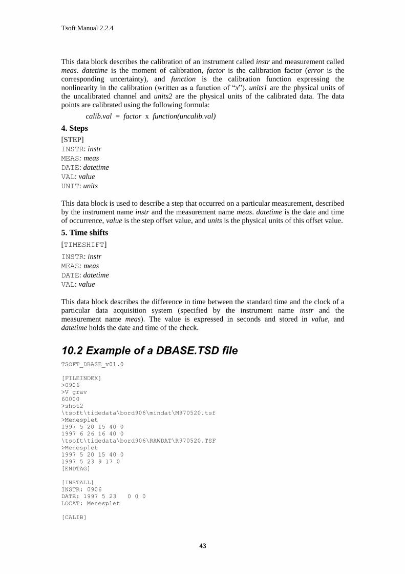
Tsoft Manual 2.2.4

43

This data block describes the calibration of an instrument called instr and measurement called

meas. datetime is the moment of calibration, factor is the calibration factor (error is the

corresponding uncertainty), and function is the calibration function expressing the

nonlinearity in the calibration (written as a function of “x”). units1 are the physical units of

the uncalibrated channel and units2 are the physical units of the calibrated data. The data

points are calibrated using the following formula:

calib.val = factor x function(uncalib.val)

4. Steps

[STEP]

INSTR: instr

MEAS: meas

DATE: datetime

VAL: value

UNIT: units

This data block is used to describe a step that occurred on a particular measurement, described

by the instrument name instr and the measurement name meas. datetime is the date and time

of occurrence, value is the step offset value, and units is the physical units of this offset value.

5. Time shifts

[TIMESHIFT]

INSTR: instr

MEAS: meas

DATE: datetime

VAL: value

This data block describes the difference in time between the standard time and the clock of a

particular data acquisition system (specified by the instrument name instr and the

measurement name meas). The value is expressed in seconds and stored in value, and

datetime holds the date and time of the check.

10.2 Example of a DBASE.TSD file TSOFT_DBASE_v01.0

[FILEINDEX]

>0906

>V grav

60000

>shot2

\tsoft\tidedata\bord906\mindat\M970520.tsf

>Menesplet

1997 5 20 15 40 0

1997 6 26 16 40 0

\tsoft\tidedata\bord906\RAWDAT\R970520.TSF

>Menesplet

1997 5 20 15 40 0

1997 5 23 9 17 0

[ENDTAG]

[INSTALL]

INSTR: 0906

DATE: 1997 5 23 0 0 0

LOCAT: Menesplet

[CALIB]

Tsoft Manual 2.2.4

44

INSTR: 0906

MEAS: V grav

DATE: 1997 5 24 17 40 0

FACT: 55.235 0.075

UNITFROM: shot2

UNITTO: nm/s^2

FUNCSTRING: x+0.015*x^2

[STEP]

INSTR: 0906

MEAS: V grav(resid) #corr

DATE: 1997 5 25 3 45 0

VAL: -43.571176

UNIT: shot2

Tsoft Manual 2.2.4

45

11. Appendix IV. The algorithms for event detection

11.1 Spikes

The detection system uses the following parameters which can be adjusted by the user:

Minimum deviation a spike should have, D

Window size W

Spike envelope E

Minimum spike / slope ratio F

Further suppose that Ai are the data points (i ranging from 0 to n-1).

1. A low pass filter FL is applied to the data points. This filter has a total length of 2W-1, and

has coefficients that decrease linearly towards the end (e.g. for W=5, the filter points are

1/25 2/25 3/25 4/25 5/25 4/25 3/25 2/25 1/25). These filtered data

points are stored in an intermediate channel Bi.

2. For each point i where the absolute value |Ai-Bi|>D, Ai is replaced by Bi. The same filter

FL is applied a second time on Ai, and the result is again stored in Bi. This complete

manipulation is repeated two times (which proves to be sufficient to have a good

convergence). The reason for this step is that very aberrant points could bias the low pass

channel Bi too much. Using this step, the spikes are already left out of the calculation. The

final values of Bi are used for the statistics (see section 0)

3. All the zones on the channel where |Ai-Bi|>D are searched on the signal. Each individual

zone is enlarged at both edges with an number of points E. If two zones turn out to be

neighbouring or even overlapping, they are merged into one single, larger zone.

4. For each zone, a linear interpolation corrector is created covering the whole zone, using

the values of Bi at both ends.

5. For each interpolation, the maximum deviation from the interpolation dmax is calculated, as

well as the absolute value of the difference between the start and end point, ds. If dmax / ds <

F, the interpolation is rejected (because it resembles more a step).

11.2 Gaps

The algorithm uses the following set of parameters, which can be chosen by the user:

The interpolation type T, which can be

1. straight connection of points using a linear interpolation

2. using a linear interpolation on fitted points

3. using a cubic interpolation on fitted points

Window size W

Polynomial degree d

Maximum gap length L (in data points)


1. All the gaps are detected.

2. If T=1, the last point before each gap and the first point after are used to create linear

interpolations and the algorithm stops.

Tsoft Manual 2.2.4

46

3. For each gap, two polynomials of degree d are fitted, one (called P1) on the last W points

before, and an other (called P2) on the first W points after the gap. If one of the

polynomials can not be fitted (e.g. because the gap occurs at the end of the file), it is

assumed to have a constant value which is equal to the closest value of the other

polynomial.

4. If T=2, a linear interpolation is created using the value of P1 at the start of the gap,

together with the value of P2 at the end of the gap.

5. If T=3, a third degree polynomial interpolation is created, using the value of P1 at the start

of the gap and its first derivative, together with the value of P2 at the end of the gap and its

first derivative.

11.3 Steps

The algorithm uses the following set of parameters, which can be chosen by the user:

Minimum deviation D

Window size W

Exclude window size V


1. At each point pj of the curve, a multi-linear regression is performed using a first degree

polynomial and a step function S(t) (S(t)= -0.5 for points to the left of pj, and S(t)= +0.5 for

the other ones). This fit is performed inside a window of 2W+1 points around the point pj,

excluding a small window of 2V+1 points around pj. This exclusion window is used the

disregard intermediate points when a step is occurring more or less slowly. The regression

coefficient of S(t) is stored in a temporary channel Bi. This channel is used for the statistics

(see section 0)

2. All the zones where |Bi|>D are identified. Each zone is enlarged with an envelope of W

points (because each step causes side lobes in Bi with negative signs), and overlapping zones

are merged.

3. For each zone, a step corrector is created having a step value, which is the maximum of Bi

inside that zone.

11.4 Statistical information

For the automatic detection of spikes and steps, it is possible to estimate the minimum

deviation in a statistical way. For each data point of the channel, the deviation value (spike or

step) is calculated using the same algorithm as for the detection of the events. A distribution

function of these values is created, and a Gaussian distribution function is fitted. Clearly, a

channel which actually contains spikes and steps will have a number of “outliers” in this

distribution, points that have a much larger deviation than can be explained by a gaussian

probability distribution.

In order to obtain the distribution of the “normal” data points, the outliers are rejected using

the following iterative procedure

1. A Gaussian distribution function is fitted

2. All points lying in the upper or lower 0.02% are removed from the distribution.

3. Using the remaining points, a new Gaussian is again fitted.

The procedure is repeated until the parameters remain unchanged.

In the dialog box of the automatic detection system, the option “diagnostics only” can be

checked in order to produce this statistics. In this case, no corrector is created, but a new

window appears, showing the distribution function of the deviations (green), as well as the

Tsoft Manual 2.2.4

47

Gaussian fit (red). In addition, a proposed limit, based on this fit, is written in the text output

window. In Figure 9, an example of a spike distribution function is shown.

Figure 9. Top row: zoom on a sample set of residuals before (left) and after (right) correction of spikes.

Bottom row: distribution function of spike values, based on the complete data set. The circles represent the distribution obtained from the observations, and the line corresponds to the Gaussian model for the “normal” points.

-10 0 10 20

Deviation (nm/s^2)

0.01

0.10

1.00

10.00

-10 0 10 20

Deviation (nm/s^2)

Tsoft Manual 2.2.4

48

12. Appendix V. Scripts in TSoft

12.1 Using scripts

In order to simplify and speed up the routine work of the processing and correction of raw

data, TSoft allows one to write simple script files that can automatically execute a number of

actions on a file. Physically, scripts are stored as files in a directory called

“\TSOFT\MACRO”.

The menu command <Script|Edit> creates the script dialog box, which shows a list of the

existing scripts. In order to add a new script, press <Add new>. The selected script can be

changed using <Edit> or deleted using <Delete>.

When a script is edited, a new dialog box appears, allowing one to enter a name for the script

and a description of the commands. In the description edit box, a new line can be taken by

pressing the CTRL+ENTER key simultaneously.

When <OK> is pressed, the program compiles the script. If a syntax error is found, an error

message is shown and the offending part of the text is highlighted.

Each script that is defined in TSoft appears as a menu command in the <Script|...> menu. In

order to run a particular script on a file, just load the file and call the appropriate menu

command.

12.2 Format of a script description

A script is a collection of function calls, each one ending with a semicolon (;). These function

calls can have arguments of three different types:

Integer values (int). These values are entered as numbers without decimal point (.).

Floating precision values (double). These values are entered as numbers with a decimal

point (.), even if they have an integer value.

Strings (string). They are entered between double quotes (").

// allows the user to enter comments (!!! Not allowed on the last line).

Some of the functions actually return a value themselves. These functions may be used as an

argument of another function (or the return value may be neglected).

To make submenus add: Submenu\macroname.

Example: We entered “hydro\Calib sondes H” to put “Calib sondes H” in the “hydro” submenu (see Figure 10).

Tsoft Manual 2.2.4

49

Figure 10. 11Example of submenus for the scripts

12.2.1 Functions supported in scripts

In the present version, the number of function calls that are supported in a script is still very

limited, and they all related to the processing and correction of raw data. The following

functions are defined:

12.2.1.1 File

exit()

to stop and exit from Tsoft

savefile(string value)

value: name of the file to which the data will be saved in TSF format

Rem: savefile(“”): save the last opened file

Openfile(string value, int type)

value: name of the file to open

type: describes the format: 1: TSF format, 2: Free, 3: GSE, 4:EVT, 5:

Preterna, 6: Free Preterna

Example: Openfile(“c:\tsoft\tidedata\sample.tsf”,1)

append(string value, int type)

value: name of the file to append

type: describes the format: 1: TSF format, 2: Free, 3: GSE, 4:EVT, 5:

Preterna, 6: Free Preterna

12.2.1.2 Edit

addcomment(string)

example: addcomment("This is my gravimeter");

This adds a comment in the header of the TSF file.

exp_channels(string value, int nr, int nr’, …)

value: name of the exported file

nr: index(es) of the channel(s) to export, separated by a comma

int addchannel ( string locat , string instr , string meas , string units )

adds a new (empty) channel to the file

locat: location name

instr: instrument name

meas: measurement name

Tsoft Manual 2.2.4

50

units: units name

return value: new channel number

delchannel ( int nr )

delete an existing channel

nr: index of the channel to delete

int dupchannel ( int nr )

creates a copy of a channel

nr: index of the channel to duplicate

return value: new channel number

mergechannels(int nr, int nc)

Merges two channels.

nr : channel read by Tsoft; if gaps (undetermined values) are found, it

fills it with the channel nc

nc: component channel used to fills gaps in the channel nr.

renchannel ( int nr , string locat , string instr , string meas , string units )

changes the name of a channel

nr: index of the channel to rename

locat: new location name

instr: new instrument name

meas: new measurement name

units: new units name

string locatof ( int nr )

gives the location of a specified channel

nr: index of the channel

return value: location name

string instrof ( int nr )

gives the instrument of a specified channel


return value: instrument name

string measof ( int nr )

gives the measurement of a specified channel


return value: measurement name

string unitof ( int nr )

gives the units of a specified channel


return value: unit name

12.2.1.3 Calculate

calcchannel ( int nr , string formula )

calculates a mathematical expression between channels (see also section 0)

nr: index of the channel to store the result

formula: description of the expression

changesamplerate ( double interval , int tpe, int window , double cutoff , string freq)

changes the sample rate of the file (see also section 0)

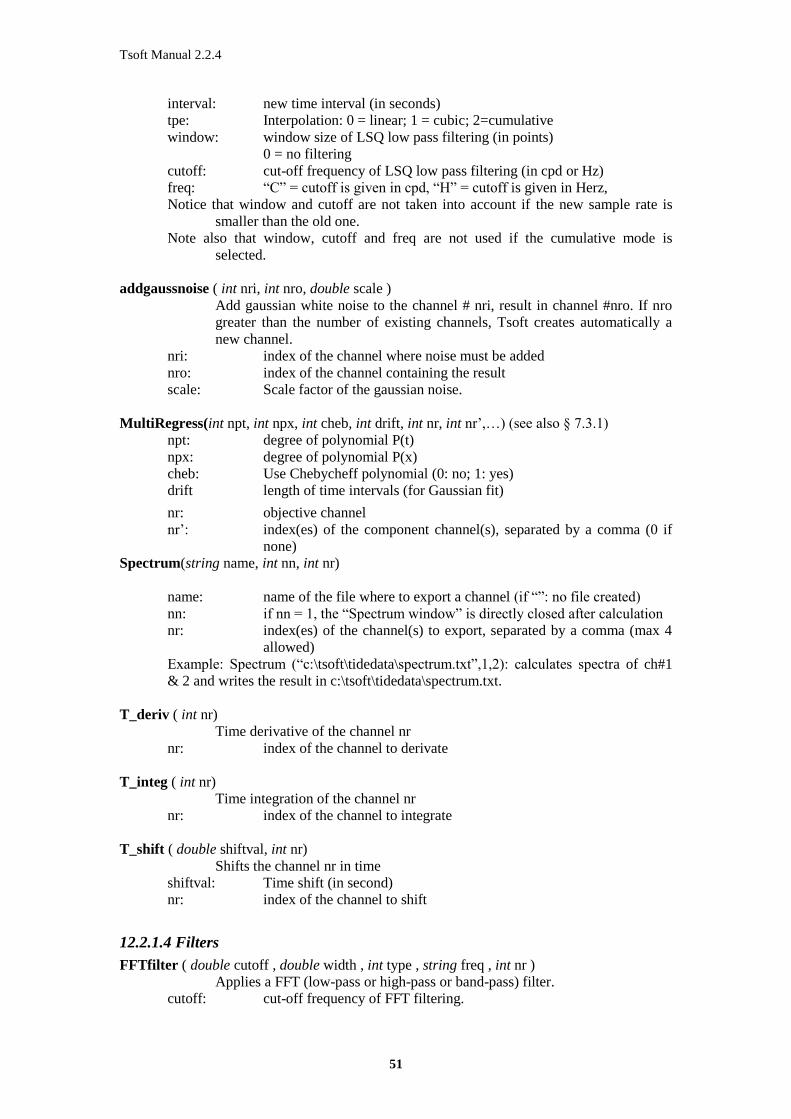
Tsoft Manual 2.2.4

51

interval: new time interval (in seconds)

tpe: Interpolation: 0 = linear; 1 = cubic; 2=cumulative

window: window size of LSQ low pass filtering (in points)

0 = no filtering

cutoff: cut-off frequency of LSQ low pass filtering (in cpd or Hz)

freq: “C” = cutoff is given in cpd, “H” = cutoff is given in Herz,

Notice that window and cutoff are not taken into account if the new sample rate is

smaller than the old one.

Note also that window, cutoff and freq are not used if the cumulative mode is

selected.

addgaussnoise ( int nri, int nro, double scale )

Add gaussian white noise to the channel # nri, result in channel #nro. If nro

greater than the number of existing channels, Tsoft creates automatically a

new channel.

nri: index of the channel where noise must be added

nro: index of the channel containing the result

scale: Scale factor of the gaussian noise.

MultiRegress(int npt, int npx, int cheb, int drift, int nr, int nr’,…) (see also § 7.3.1)

npt: degree of polynomial P(t)

npx: degree of polynomial P(x)

cheb: Use Chebycheff polynomial (0: no; 1: yes)

drift length of time intervals (for Gaussian fit)

nr: objective channel

nr’: index(es) of the component channel(s), separated by a comma (0 if

none)

Spectrum(string name, int nn, int nr)

name: name of the file where to export a channel (if “”: no file created)

nn: if nn = 1, the “Spectrum window” is directly closed after calculation

nr: index(es) of the channel(s) to export, separated by a comma (max 4

allowed)

Example: Spectrum (“c:\tsoft\tidedata\spectrum.txt”,1,2): calculates spectra of ch#1

& 2 and writes the result in c:\tsoft\tidedata\spectrum.txt.

T_deriv ( int nr)

Time derivative of the channel nr

nr: index of the channel to derivate

T_integ ( int nr)

Time integration of the channel nr

nr: index of the channel to integrate

T_shift ( double shiftval, int nr)

Shifts the channel nr in time

shiftval: Time shift (in second)

nr: index of the channel to shift

12.2.1.4 Filters

FFTfilter ( double cutoff , double width , int type , string freq , int nr )

Applies a FFT (low-pass or high-pass or band-pass) filter.

cutoff: cut-off frequency of FFT filtering.

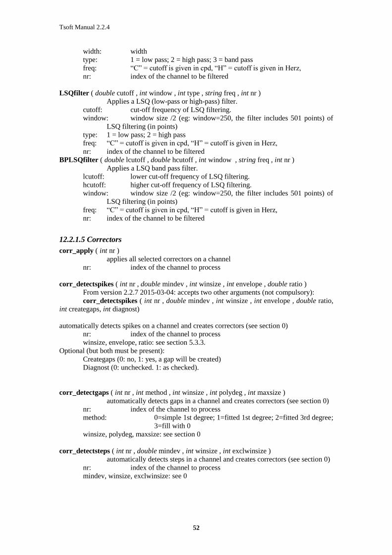
Tsoft Manual 2.2.4

52

width: width

type: 1 = low pass; 2 = high pass; 3 = band pass


nr: index of the channel to be filtered

LSQfilter ( double cutoff , int window , int type , string freq , int nr )

Applies a LSQ (low-pass or high-pass) filter.

cutoff: cut-off frequency of LSQ filtering.

window: window size /2 (eg: window=250, the filter includes 501 points) of

LSQ filtering (in points)

type: 1 = low pass; 2 = high pass



BPLSQfilter ( double lcutoff , double hcutoff , int window , string freq , int nr )

Applies a LSQ band pass filter.

lcutoff: lower cut-off frequency of LSQ filtering.

hcutoff: higher cut-off frequency of LSQ filtering.

window: window size /2 (eg: window=250, the filter includes 501 points) of

LSQ filtering (in points)



12.2.1.5 Correctors

corr_apply ( int nr )

applies all selected correctors on a channel

nr: index of the channel to process

corr_detectspikes ( int nr , double mindev , int winsize , int envelope , double ratio )

From version 2.2.7 2015-03-04: accepts two other arguments (not compulsory):

corr_detectspikes ( int nr , double mindev , int winsize , int envelope , double ratio,

int creategaps, int diagnost)

automatically detects spikes on a channel and creates correctors (see section 0)


winsize, envelope, ratio: see section 5.3.3.

Optional (but both must be present):

Creategaps (0: no, 1: yes, a gap will be created)

Diagnost (0: unchecked. 1: as checked).

corr_detectgaps ( int nr , int method , int winsize , int polydeg , int maxsize )

automatically detects gaps in a channel and creates correctors (see section 0)


method: 0=simple 1st degree; 1=fitted 1st degree; 2=fitted 3rd degree;

3=fill with 0

winsize, polydeg, maxsize: see section 0

corr_detectsteps ( int nr , double mindev , int winsize , int exclwinsize )

automatically detects steps in a channel and creates correctors (see section 0)


mindev, winsize, exclwinsize: see 0

Tsoft Manual 2.2.4

53

12.2.1.6 Data base

chgdatabase (string databasename)

change the databasename

copystepstodbase ( int nr )

copies all applied steps to the instrument database


applysteps (int nr)

applies all selected steps contained in the database on a channel


savedatabase()

save the data base into the file specified in “chgdatabase”

Example:

chgdatabase("c:\mydirectory\mydatabase\MyBestInstrument.tsd");

corr_detectsteps(1, 2. ,10, 1 );

corr_apply(1);

copystepstodbase(1);

savedatabase();

After step detection, then application, the script copies them to the data base

“MyBestInstrument.tsd” and saves it.

12.2.1.7 Tides

calcsynthtide ( string locat , string tide )

creates a new channel containing a synthetic tide

locat: location of the requested tide

tide: name of the requested tide

12.2.1.8 Varia

setpar(int nr, string value):

allocates the value contained in the string “value” to the parameter # “nr”

double getpar(int nr)

calls the parameter # “nr” and returns its value

calibrate ( int nr , string units )

calibrates a channel into new units

nr: index of the channel to calibrate

units: units of the calibrated data

12.2.2 An example of a script containing getpar and setpar

setpar(1,"3.14"); //parameter #1 = 3.14

setpar(2,"2.0"); // parameter #2 = 2.0

setpar(3,"getpar(1)*getpar(2)"); //parameter #3=2*3.14

Tsoft Manual 2.2.4

54

setpar(4, "getpar(3)^2"); //parameter #4=(2*3.14)²

calcchannel(1,"sin(getpar(4)*t)"); //channel 1 gives the function sin((2*3.14)²*t)

exit();

12.3 Calling a script from Windows command line

The syntax is:

c:\Tsoft\tsoft.exe [data file to be opened] [/s script name]

This runs Tsoft, opens the selected data file and applies the script.

The scripts must have been already recorded. If no script is mentioned, then Tsoft just opens

the data file.

!!! The data file to be open is optional because the script itself may contain the Openfile

instruction.

Example:

Your script is cv min->hour to decimate data. It contains this command:

changesamplerate(3600.0,0,600,12.0,"C");

Then

c:\Tsoft\tsoft.exe [c:\MyData\myfile.tsf] [/s cv min->hour]

will change the sampling rate of the data contained in myfile.tsf.

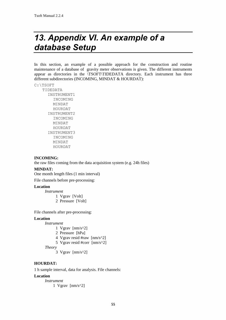
Tsoft Manual 2.2.4

55

13. Appendix VI. An example of a database Setup

In this section, an example of a possible approach for the construction and routine

maintenance of a database of gravity meter observations is given. The different instruments

appear as directories in the \TSOFT\TIDEDATA directory. Each instrument has three

different subdirectories (INCOMING, MINDAT & HOURDAT):

C:\TSOFT

TIDEDATA

INSTRUMENT1

INCOMING

MINDAT

HOURDAT

INSTRUMENT2

INCOMING

MINDAT

HOURDAT

INSTRUMENT3

INCOMING

MINDAT

HOURDAT

INCOMING:

the raw files coming from the data acquisition system (e.g. 24h files)

MINDAT:

One month length files (1 min interval)

File channels before pre-processing:

Location Instrument

1 Vgrav [Volt]

2 Pressure [Volt]

File channels after pre-processing:

Location Instrument

1 Vgrav [nm/s^2]

2 Pressure [hPa]



Theory

3 Vgrav [nm/s^2]

HOURDAT:

1 h sample interval, data for analysis. File channels:

Location Instrument

1 Vgrav [nm/s^2]

Tsoft Manual 2.2.4

56

2 Pressure [hPa]

Theory

3 Vgrav [nm/s^2]

13.1 Set of script files used for processing the data

In the remainder of this section, a set of scripts for the routine reduction and correction of raw

gravity data is presented. It is supposed that the raw data files has two channels, the first one

containing the vertical gravity, and the second one containing the air pressure (both

uncalibrated). The channel window looks like:

Location Instrument

1 Vgrav [Volt]

2 Pressure [Volt]

13.1.1 Calibration of the data

The script “calibrate” is used for the calibration of both channels

calcchannel(1,"[1]*12.5223");

renchannel(1,locatof(1),instrof(1),measof(1),"nm/s^2");

calcchannel(2,"[2]*87.5221");

renchannel(2,locatof(2),instrof(2),measof(2),"hPa");

The calibration could have been done using the instrument database and the function

“calibrate”, but if the sensitivity does not change in time, it can be done with a simple

function evaluation.

13.1.2 Calculation of the residuals

The script “calc_residuals” adds the theoretical tide to the file and calculates the residuals

(assuming that a tide “Vgrav” is present for the location).

calcsynthtide(locatof(1),"Vgrav");

addchannel(locatof(1),instrof(1),"Vgrav resid #raw",

unitof(1));

calcchannel(4,"[1]-[3]+3.2*[2]");

dupchannel(4);

renchannel(5,locatof(5),instrof(5),"Vgrav resid

#corr",unitof(5));

The pressure admittance factor is 3.2, but can be changed easily.

The channels now look like

Location Instrument

1 Vgrav [nm/s^2]

2 Pressure [hPa]



Theory

3 Vgrav [nm/s^2]

Tsoft Manual 2.2.4

57

13.1.3 Correction of events

At this moment, the spikes, steps and gaps should be removed from the residuals. Preferably,

this should be done in an interactive way. However, it can be done completely automatically

by a script “correctevent”, too:

corr_detectspikes(5,10.0,50,5,3.0);

corr_apply(5);

corr_detectgaps(5,2,50,1,1500);

corr_apply(5);

corr_detectsteps(5,20.0,50,5);

corr_apply(5);

13.1.4 Calculation of the corrected tide

When the residuals are corrected, the corresponding tide can be calculated using the script

“restoretide”:

calcchannel(1,"[3]+[5]-3.2*[2]");

13.1.5 Reduction of the sample rate.

The last script “reducesample”, removes the channels containing the residuals, and reduces

the sample rate to a 1 hour interval. After application of this script, the file should of course

be stored under an other name or in a different directory.

delchannel(3);

delchannel(3);

delchannel(3);

changesamplerate(3600,480,12.0);

Tsoft Manual 2.2.4

58

14. Appendix VII. Calculating transfer function using step functions and sine waves

Step functions

If one injects a step voltage into an instrument, it is possible to get its frequency transfer

function by calculating the Fourier spectrum of the differentiated step response function.

Earth tides (and other drifts) must be removed from the recording before analysis.

Select the channel by highlighting it (cf. § 3.1.1). Let us suppose we analyse 4 minutes after

the step. First make inactive the points following the 4 minutes (cf. § 3.2.4) (it is not

necessary to inactivate all the following data). Then position the curve cursor (red cross) at

the beginning of the step and use the <Calculate|Transfer function> command. Two

windows appear: “Transfer function (normalised amplitude)” and “Transfer function (group

delay)”. The first one gives the amplitude response, normalised with the amplitude at the

lowest frequency. The second one gives the group delay in second, with the curve cursor as

origin time. The delays appearing at frequencies higher than the corner frequency are

meaningless. The numerical values may be exported using <File|Export>.

!!! Important remarks:

1) Analysing a perfect step (i.e. a direct jump from 0 to, say, 1) produces a fatal error.

2) The step must be upward. If you want to analyse downward steps, first reverse the

channel sign by using <Calculate|Evaluate expression> (cf. 3.3.2).

3) Applying a Least Squares Filter (§ 7.2.2) before analysing steps may improve the group

delay results.

Sine waves

By fitting both the input (injected sine waves) and the output signals (instrument response) on

the function a T t T b T t T P t( )sin( / ) ( )cos( / ) ( )2 2 6 , one obtains the phase and

amplitude response of the instrument at the period T. P6(t) is a 6th degree polynomial

necessary to remove Earth tides and other drifts. Removing Earth tides by subtraction of a

synthetic tide gives similar results. The amplitude ratios and the phase differences of the fitted

input and output sinusoidal waves provide the instrumental transfer function.

To fit the input channel, highlight this channel then click the <Calculate|Fit Sinus> menu. A

dialog box asks the period T of the sine wave. Press <OK> and another box asks the

polynomial degree. Press <OK> and the function

a T t T b T t T P t( )sin( / ) ( )cos( / ) ( )2 2 6 is fitted on the selected channel. Select now the

output channel that contains the instrument response to the injected sine waves and do a new

fit with <Calculate|Fit Sinus>. The results are now in the text output window.

For all fits, the text output window gives the correlation and the standard deviation, which

allow easily one to check the fit (e.g., if the chosen period T is the right one). For all fit, the

text output gives also the amplitude a, b and the error of the fitted sine and cosine, as well as

the amplitude a b² ² and the phase tan1 a b . Then, the following text looks like:

Tsoft Manual 2.2.4

59

PROP WITH PREVIOUS:

AMP 123.123 PHA 123.12 s

0.123 s 0.12

This is the amplitude ratio between the input and the output, the phase difference and their

respective error. These errors result from the least squares fit on the output channel (more

exactly: on the last fitted channel). Note that this appears after each fit but has only a

signification after the second one.

Evaluating the noise effect on sine waves by bootstrapping

As steps are easy to repeat, we can look at the standard deviation to assess the noise effect.

For long period sine waves, it is difficult to perform several experiments, so a bootstrap

method (Monte-Carlo simulation) can be useful.

This method consists of producing a noise with a spectrum similar to the real one affecting the

measurements. This noise is obtained after calculation of the residuals after fitting a function

on an instrumental data set. The smoothed power spectrum of the residuals is multiplied by a

Gaussian white noise, which gives a spectrum whose inverse Fourier transform produces a

colored noise similar to the real one. A mathematical sine is added. The resulting signal is

analysed in the same way as the instrumental data. This procedure is repeated 1000 times for

a given period. This gives an error distribution function of the amplitude response and the

time lag for this period.

Detailed procedure:

A. Creating the artificial noise

1) take the output channel that contains the instrument response to a sine wave of period T

(it should be a representative recording (more than 1 hour long)).

2) Create two new channels, one with sin( * * * / )2 t N T and the other one with

cos( * * * / )2 t N T (N is the number of point in one day. e.g. 86400 if sampling rate =

1s).

3) Using <Calculate|Multilinear regression> fit the output on those two channels, using a

6th degree polynomial P(t).

4) With <Calculate|Evaluate spectrum> calculate the spectrum of the residual of the fit.

5) Select <Spectrum|Show cycles per day> and calculate the smoothed power spectrum

with <Spectrum|Spectral Power Table>. Frequency increment should be 300 and

Maximum frequency 30000 cpd.

6) Save this power spectrum by using <File|Export> in the spectral power window.

7) The window "Spectral Power" appears. Select then <Calculate|Create colored noise>: a

new channel is created, which contains the noise similar to the real one.

8) To normalise the colored noise with the real one, calculate the spectrum of both and for

each spectrum, calculate <Spectrum|Spectral power inside window>. The result

appears in the “Text output” window:

POWER OF 1: xxxxx

POWER OF 2: xxxxx

B. Monte Carlo simulation

1) Open the file corresponding to an experiment

2) With <Calculate|Fit Sinus>, evaluate the amplitude of the sine wave (given in the “Text

output” window).

3) <Others|Plug-ins|MC simuls of sin fit> :

Tsoft Manual 2.2.4

60

1- Enter amplitude: this is the amplitude of

the sine Wave calculated in the previous

point

2- Enter period (s): this is the period of the

injected wave

3- Enter # of simuls: this is the number of

MC simulations (e.g. 1000)

4- Enter noise file: this is the file that

contains the noise power spectrum (file

created in A.6)

5- Enter factor for noise: this is the ratio

between the power spectrum of the real

data and the coloured noise one (cf.. A.7)

6- Set thread at low priority: if you answer

yes, the MC simulation shall work more

slowly. This could be useful if you want

to do something else during the

calculation.

4) A file out.txt is created, containing the noise simulation on the amplitude and phase

calculation. <Calculate|Histogram> allows to calculate a histogram, giving the

distribution function. The “Text output” gives the mean, the standard deviation and the

intervals where 68, 95.5 and 99.7% of the results lie.

Acknowledgements

We thank the numerous users of Tsoft for their patience and help in improving the software

and the manual. Special thanks to Olivier de Viron, Olivier Francis, Marc Hendrickx Peter

Wolf and Hartmut Wziontek for fruitful comments and suggestions, and to Hans-Georg

Scherneck for providing the ocean loading parameters into the Tsoft format. Finally we

thanks Henri Martin for his valuable help in C++.

References

Hartmann, D.L. & Michelsen, M.L., Intraseasonal Periodicities in Indian Rainfall, J. Atm.

Sci., 46(18), 2838-2862? 1989.

Richter, B. and Wenzel, H.-G.? Precise instrumental phase lag determination by the step

response method. Bull. Inf. Marées Terrestres, 111, 8032-8052, 1991.

Van Camp, M., Wenzel, H.-G., Schott, P., Vauterin, P. and Francis, O., Accurate transfer

function determination for superconducting gravimeters. Geophysical Research Letters,

27, 1, 37-40, 2000.

Von Storch, H., & Zwiers, F.W., Statistical analysis in climate research, Cambridge

University Press, Cambridge, 484pp, 1999.

Wenzel, H.-G., Accurate instrumental phase lag determination for feedback gravimeters.

Proc. 12th Int. Symp. Earth Tides, 191-198, H.T. Hsu (ed.), Science Press, Beijing, New-

York, 1995.

Tsoft Manual 2.2.4

61

15. Appendix VIII. Calculating gravity gradient

The command <Tides|gravity gradient> allows one to calculate easily the vertical gravity

gradient using a spring gravimeter. It works exactly like the <calculate|multilinear

regression> command; it needs as objective channel (highlighted) the gravity and as

component channel (in red) the levels. It is possible to fit a temporal drift (linear, quadratic,

…), as well as a height dependence (only linear or quadratic). The text output window gives

the gradient (at the levels 65 & 90cm if the height dependence is quadratic) and statistical

information (correlation matrix, …).

tsoft manual

Documents