tsagas
TRANSCRIPT
1
University of Strathclyde Energy Systems Research Unit MSc “Energy Systems & the Environment”
MSc’s Dissertation Title
LABORATORY EVALUATION OF DC / AC INVERTERSFOR STAND-ALONE & GRID-CONNECTED
PHOTOVOLTAIC SYSTEMS
The present research project has been supported from the Center for Renewable Energy Sources in Greece
Mr Ilias Tsagas email: [email protected] © 2002
2
Introduction
The present dissertation is the result of my individual research activity during the third
part of the Strathclyde University’s MSc course “Energy Systems & the Environment”.
It includes experimental laboratory evaluation of a DC to AC stand-alone inverter as
well as of a DC to AC grid-connected inverter, while the development of my
experimental activity has been carried out at the Department of Photovoltaic Systems,
in the Centre for Renewable Energy Sources (C.R.E.S) in Greece.
The first step of my work was the configuration of the inverters test circuits, at the
Power Electronic Lab of the Photovoltaic Department. The necessary stuff was
provided by C.R.E.S.
The first part of the experiment concerns the measurement of the Trace Engineering
stand-alone inverter’s (model 2524, 2.5 kW) efficiency. The inverter was connected
firstly at its output terminals with a resistive load, in order to measure its efficiency, at
the inverter’s input voltage equal to the inverter’s nominal input voltage. At the same
input voltage, the no-load and standby losses of the inverter, the output current ripple
and the total harmonic distortion (THD) of both current and voltage were also
measured. Measurements have been carried out for many different power levels of the
resistive output load, while in order to produce the necessary input voltage of the
inverter; we used four batteries of 12 V each.
Efficiency of the inverter was measured after again, with a reactive load connected at
the inverter’s output terminals. Efficiency was namely measured with a load, which
provides power factors 0.25, 0.50 and 0.75 and for many different power levels of the
reactive output load. All the other sizes have been also measured as before.
The second part of the experiment concerns the measurement of the Total Energie grid-
connected inverter (model Onbuleur Joule Prg, 2.5 kW). The previous experimental
test circuit was used again, but now the inverter was connected at the grid and instead
of batteries, power supplies were used. At three inverter’s input voltages, equal to the
manufacturer’s minimum rated input voltage, the inverter’s nominal voltage and the 90
% of the inverter’s maximum input voltage respectively, the same sizes as in stand-

3
alone inverter were measured again. At this case, the harmonic currents and voltages
injected into grid by the inverter were further recorded.
The above work has been presented analytically at the next pages of this paper.
Namely, the first chapter of the dissertation is an introduction about the inverters, in
order readers to obtain a view of the subject. The second chapter describes step by step
the measuring procedure that has been followed and the stuff that was used to set up
the test circuits, while the third chapter includes the results of the experiment and
author’s conclusions.
The present paper can be used in future from students and institutes, as a basis for the
production of relative work.
4
Table of Contents
1. Chapter 1, INVERTERS: AN INDRODUCTION… … .… … … ...… … … … … 6
A. STAND-ALONE INVERTERS… … … … … … … … … … … … … .… … … … ....… 6
B. GRID-CONNECTED INVERTERS… … … … … … … … … … … … … … .… ....… .9
C. WHERE DOES ANY EXCESS ENERGY GO?… … … … … … … … .… … … … 13
D. WHO NEEDS A GENERATOR?… … … … … … … … … … … … … .… … … … ..13
E. EFFICIENCY… … … … … … … … … … … … … … … … … … … … … … .… … … ..14
F. SIZING… … … … … … … … … … … … … … … … … … … … … … … … .… … … … 14
G. SITING… … … … … … … … … … … … … … … … … … … … … … … … … … … … .15
2. Chapter 2, EXPERIMENT WE DO… … .… … … … … … … … … … … … … ....16
A. PROCEDURE FOR MEASURING EFFICIENCY… … … … … … … … … .… ...16
A1. DEFINITIONS… … … … … … … … … … … … … … … … … … … … … .… … ...16
A2. EFFICIENCY MEASUREMENT CONDITIONS… … … … … … … … … … .17
A3. READINGS TO BE RECORDED… … … … … … … … … … … … … … … … ..18
A3.1 Ripple and distortion… … … … … … … … … … … … … … … … … … … … .18
A3.2 Resistive loads / utility grid… … … … … … … … … … … … … … … … … ...18
A3.3 Reactive loads… … … … … … … … … … … … … … … … … … … … … … ...19
A3.4 Loss measurement… … … … … … … … … … … … … … … … … … … … … .19
A3.5 Harmonic Components… … … … … … … … … … … … … … … … … … … ..19
A4. EFFICIENCY CALCULATIONS… … … … … … … … … … … … … … … … ..19
B. EFFICIENCY TEST CIRCUITS… … … … … … … … … … … … … … … … … … .21
B1. TEST CIRCUITS… … … … … … … … … … … … … … … … … … … … … … ...21
B2. EQUIPMENT OF THE TEST CIRCUITS… … … … … … … … … … … … … 22
B2.1 Equipment of the stand-alone inverter’s test circuit… … … … … … … … .22
B2.2 Equipment of the grid-connected inverter’s test circuit… … … … … … ...24
B2.3 Measurement procedure… … … … … … … … … … … … … … … … … … ...26
C. INVERTERS, WHICH ARE TESTED… … … … … … … … … … … … … … … ....29
C1. STAND-ALONE TYPE… … … … … … … … … … … … … … … … … … … … .29
C2. GRID-CONNECTED TYPE… … … … … … … … … … … … … … … … … … ..31

5
3. Chapter 3, RESULTS & CONCLUSIONS… … … … … … … … … … … … … ..33
A. STAND-ALONE INVERTER’S TEST RESULTS… … … … … … … … … … … 33
A1. TEST WITH RESISTIVE LOAD-
INVERTER’S EFFICIENCY AT NOMINAL INPUT VOLTAGE, 24 V...33 A2. TEST WITH REACTIVE LOAD-
INVERTER’S EFFICIENCY AT NOMINAL INPUT VOLTAGE, 24 V...40
A2.1 For Power factor (cosϕ) 0,25… … … … … … … … … … … … … … … … ...40
A2.2 For Power factor (cosϕ) 0,50… … … … … … … … … … … … … … … … ...42
A2.3 For Power factor (cosϕ) 0,75… … … … … … … … … … … … … … … … ...45
A3. LOSS MEASUREMENT TEST RESULTS… … … … … … … … … … … … .49
A4. CONCLUSIONS… … … … … … … … … … … … … … … … … … … … … … ...50
B. GRID-CONNECTED INVERTER’S TEST RESULTS… … … … … … … … … .52
B1. INVERTER’S EFFICIENCY AT MINIMUM RATED INPUT VOLTAGE
B2. INVERTER’S EFFICIENCY AT NOMINAL INPUT VOLTAGE… … … ..58
B3. INVERTER’S EFFICIENCY AT MAXIMUM INPUT VOLTAGE… … … 64
B4. LOSS MEASUREMENT TEST RESULTS… … … … … … … … … … … … ..67
B5. HARMONICS… … … … … … … … … … … … … … … … … … … … … … … … 68
B6. CONCLUSIONS… … … … … … … … … … … … … … … … … … … … … … … 73
4. In Conclusion… … … … … … … … … … … … … … … … … … … … ...… … … … ...75
5. Acknowledgements… … … … … … … … … … … … … … … … … … … … … … … .76
6. References… … … … … … … … … … … … … … … … … … … … … … … … … … ...77

6
Chapter 1
INVERTERS: AN INTRODUCTION
What does an inverter do?
Inverters are power electronic devices, which convert DC (typically low voltage)
into AC (at 230 V, 50 Hz) as required for conventional appliances. There are
generally two types of photovoltaic inverter available: stand-alone and grid-
connected.
A. STAND-ALONE INVERTERS
Stand-alone, or battery supplied, inverters are demand driven - they provide any power
or current up to the rating of the inverter and assuming that there is enough energy in
the battery.
These inverters are being used increasingly to operate household appliances and other
“normal” 230 V equipment. The question as to the maximum size for which a single
central inverter for all electrical devices is still the best solution, is a matter of
philosophy. The central inverter must be in operation all the time. In this case, it is
important that the inverter itself has a very low internal consumption.

7
Different types of inverter produce different AC waveforms and are suitable for
different situations.
Square Wave Inverters
The square wave inverter derives its name from the shape of the output waveform (see
figure 1).
Figure 1- Square Wave Output Wave
Square wave inverters were the original “electronic” inverter. The first versions use a
mechanical vibrator type switch to break up the low voltage DC into pulses. These
pulses are then applied to a transformer where they are stepped up. With the advent of
semiconductor switches the mechanical vibrator was replaced with “solid state”
transistor switches. Nowadays, the most common circuit topology, which is used to
produce a square wave output, referred to as “push-pull”.
Square wave inverters run simple electric motors, but not much else, and will require a
lot of energy to do so. Also, this kind of inverters is low quality. The price of better
quality inverters is low enough to make the use of these unattractive.
Modified Square Wave Inverters
Modified square wave inverters (often referred to as modified sine wave inverters) use
a push-pull topology as well as square wave inverters, with the addition of a few extra
parts in their design. However, some modified square wave inverters use another one
topology, which is called “H-Bridge”. Their output has the shape of the waveform of
the next page (see figure 2).

8
Figure 2- Modified Square Wave
These inverters are a good choice for a 'whole home' inverter since their high surge
capacity lets them start motors whilst their high efficiency lets them run small
appliances economically.
Most loads will run without trouble from a modified sine wave. It is suitable for a
variety of applications such as induction motors (i.e. refrigerators, drill presses);
resistive loads (i.e. heaters, toasters); universal motors (i.e. hand tools, vacuum
cleaners) as well as microwaves and computers. However, some appliances will not
operate or will run noticeably less well if not on a pure sine wave.
Problem loads: e.g. many laser printers, copiers, some computers, light dimmers and
some variable speed tools may not operate; some TV's and some audio equipment will
pick up interference or background buzz; some digital clocks may not keep time;
microwave ovens will have longer cooking times; and some small battery chargers
may fail. Central heating ignition systems can be problematic.
Sine Wave Inverters
A sine wave inverter puts out an AC equal to what you get from utility grid, a smooth
sine wave. A 'mains' quality pure sine wave output is necessary for some applications
such as running electronics or audio equipment.
Two common tolopogies that are used to produce sine wave output are push-pull and
H-Bridge.
True sine wave inverters can run all types of load and are now available which are
powerful, efficient and affordable! Their disadvantage is their cost, which is higher
than the cost of the other kinds of inverters.
Zero or“Off Time”band
Pulseheight

9
B. GRID-CONNECTED INVERTERS
Grid-connected inverters are supply driven - they provide all the power supplied from a
DC source to the grid or mains. Therefore, in grid-connected systems, the solar inverter
is the connecting link between the solar generator and the AC grid, while the
characteristics of the inverter have a decisive influence on the performance of the grid-
connected photovoltaic system.
Generally, grid-connected inverters operate at a higher DC voltage than stand alone
inverters.
Grid-connected inverters should NOT be connected to batteries and stand-alone
inverters should NOT be connected directly to PV or the grid.
Smaller systems with few appliances may have only DC power, but recent advances in
inverter design, efficiency, and reliability have increased the potential of solar systems
considerably.
With the use of modern high efficiency AC lighting the majority of, if not all, loads
can be operated on AC especially in larger installations.
We can use both AC & DC where each is most effective and economical - many DC
appliances use less power than their AC equivalents (especially refrigeration, lighting
& electronics) - but DC appliances tend to be harder to find and more expensive.

10
How do they work?
The grid-connected inverter must convert the direct current from the solar modules to
alternating current synchronous with the grid.
It must also be optimally matched to the I-V characteristic of the solar generator.
Therefore, in PV applications the inverter will automatically adjust the PV array
loading to provide peak efficiency of the solar panels by means of maximum power
point tracking (MPPT).
Inverters automatically shutdown in the event of:
• High/Low grid AC-voltage
• High/Low grid frequency
• Grid Failure
• Inverter malfunction
Technicalities
Connection of a photovoltaic electrical system to the electricity grid must have local
electricity company approval and installation method and protection must meet their
safety requirements and appropriate standards.
There are costs associated with connection and metering to/from the grid. Also, the rate
paid for electricity generated is usually considerably less than that charged for
electricity consumed. Thus, the best economics are obtained if all the power generated
can be consumed on site.
11
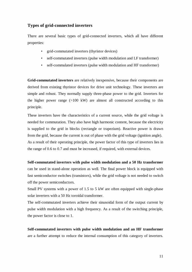
Types of grid-connected inverters
There are several basic types of grid-connected inverters, which all have different
properties:
• grid-commutated inverters (thyristor devices)
• self-commutated inverters (pulse width modulation and LF transformer)
• self-commulated inverters (pulse width modulation and HF transformer)
Grid-commutated inverters are relatively inexpensive, because their components are
derived from existing thyristor devices for drive unit technology. These inverters are
simple and robust. They normally supply three-phase power to the grid. Inverters for
the higher power range (>100 kW) are almost all constructed according to this
principle.
These inverters have the characteristics of a current source, while the grid voltage is
needed for commutation. They also have high harmonic content, because the electricity
is supplied to the grid in blocks (rectangle or trapezium). Reactive power is drawn
from the grid, because the current is out of phase with the grid voltage (ignition angle).
As a result of their operating principle, the power factor of this type of inverters lies in
the range of 0.6 to 0.7 and must be increased, if required, with external devices.
Self-commutated inverters with pulse width modulation and a 50 Hz transformer
can be used in stand-alone operation as well. The final power block is equipped with
fast semiconductor switches (transistors), while the grid voltage is not needed to switch
off the power semiconductors.
Small PV systems with a power of 1.5 to 5 kW are often equipped with single-phase
solar inverters with a 50 Hz toroidal transformer.
The self-commutated inverters achieve their sinusoidal form of the output current by
pulse width modulation with a high frequency. As a result of the switching principle,
the power factor is close to 1.
Self-commutated inverters with pulse width modulation and an HF transformer
are a further attempt to reduce the internal consumption of this category of inverters.

12
Ferrite transformers ensure the galvanic separation of the grid and the solar generation
here.
The switching concept of these inverters requires three stages with power
semiconductors. This means two more stages than for pulse width modulated solar
inverters with an LF transformer. However each additional stage can cause further
losses if it is not optimised. That is a main reason why the original aim to increase the
efficiency by incorporating HF technology has not succeeded convincingly.

13
C. WHERE DOES ANY EXCESS ENERGY GO?
This depends on whether the system is stand-alone or whether it is grid-connected.
Storage batteries are the heart of all stand-alone PV or inverter electrical systems.
By storing excess energy when the sun is strong, they offer a reliable source of
electricity, which can be used when solar power is not available.
Their function is therefore to balance the outgoing electrical requirements with the
incoming energy supply.
Batteries are also able to provide short-term power output, many times higher than the
charging source output.
For grid-connected inverters, energy is fed back into the grid.
D. WHO NEEDS A GENERATOR?
In typical domestic situations, for most of the day, loads are very small - perhaps a few
lights and other appliances.
For a small proportion of the time, however, large loads such as washing machines,
electric kettles, etc. must be powered.
Sizing a renewable energy system to meet this peak demand is, in most cases,
prohibitively expensive (at least initially).
The optimum way to incorporate a solar energy is for this to supply the low loads
required for most of the day, and allow a generator to start up automatically to meet the
small proportion of loads for which a large capacity is required.
In such systems, batteries allow power to be available 24 hrs/day but means that the
generator need only run for short periods to charge the battery.
14
E. EFFICIENCY
Modern electronic inverters are very efficient over a wide range of outputs, but some
power is required simply to keep the inverter running (the standing losses) and they are
less efficient when running small loads.
Consequently, sizing the inverter for its required purpose is extremely important.
þ If it is undersized, then there will not be enough power - demanding more than
their limit will shut them off.
þ If it is oversized, it will be much less efficient (due to the standing losses) and
more costly to buy and run.
A load seeking circuit is normally included to ensure that battery power is conserved
for useful purposes by automatically switching the inverter on and off as loads are
applied or discontinued.
F. SIZING
In inverter sizing the most important factor is peak power consumption: the peak
power demand should not exceed the rated peak output of the inverter.
This is difficult when it is possible for many devices to consume power at the same
time, and is further complicated by any electric motors in the system.
Some types of electric motors require three times as much power to start them as is
required to run them. If two or more motors are started at the same time the surge
power demand is much higher than the average demand. Consequently, the inverter
should be sized to be able to at least start the largest motor in the system and measures
taken to ensure that all motors do not start at the same time.
Proper energy management can reduce peak demand, and so the inverter can be sized
closer to the average power demand, thereby increasing the system's efficiency and
reducing hardware costs.

15
G. SITING
Inverters should be located in a dry, non-condensing, clean, ventilated environment.
Vented lead acid batteries can produce corrosive vapors and when on charge produce
an explosive mixture of hydrogen and oxygen. So, good ventilation is required for the
battery, particularly at a high level to allow any hydrogen to disperse.
Preferably, the battery should be in it’s own cubicle, vented to the outside. If this is not
practicable, we don’t mount the inverter directly above the battery or directly adjacent
to it.
In order to minimize the voltage drop in the connecting cables to the battery, these
should be kept as short as possible and of sufficient size.

16
Chapter 2
EXPERIMENT WE DO
The main activity of the present project was to measure the efficiency of two different
types of inverters, which are used in stand-alone and utility-interactive photovoltaic
systems, respectively. Further tests, in order to measure the no-load and stanby losses
of the inverters have been made, while the harmonic currents and harmonic voltages,
which are injected into grid by the grid-connected inverter, are measured as well.
The goal was after we complete our tests and based on the measurements, to be able to
have a clear view of the performance of the specific models of inverters.
The procedure for measuring the efficiency of the inverters, which are used in stand-
alone and utility-interactive photovoltaic systems, is based on the International
Electrotechnical Commission’s Standard 61683 “Photovoltaic systems-Power
Conditioners-Procedure for measuring efficiency”.
A. PROCEDURE FOR MEASURING EFFICIENCY
A1. DEFINITIONS
For the purposes of the present project (as well as of the IEC 61683), the following
definitions apply. All efficiency definitions are applied to electric power conversion
alone and they do not consider any heat production.
17
• rated output efficiency: ratio of output power to input power, when the
inverter is operating as its rated output.
• partial output efficiency: ratio of output power to input power, when the
inverter is operating below its rated output.
• no-load loss: input of the inverter, when its load is disconnected or its output
power is zero.
• standby loss: for a utility interactive inverter, power drawn from the utility grid
when the inverter is in standby mode. For a stand-alone inverter, d.c. input
power when the inverter is in standby mode.
A2. EFFICIENCY MEASUREMENT CONDITIONS
Efficiency of the inverters has been measured under the below conditions:
• DC power source for testing
For inverters operating with fixed input voltage, the d.c. power source was a storage
battery or constant voltage power source to maintain the input voltage.
• Temperature
According to the IEC 61683 standards, all measurements are to be made at an ambient
temperature of 25 °C ± 2 °C. However, there wasn’t control of the temperature during
our measurements. The ambient temperature in our case was the typical room
temperature.

18
• Output voltage and frequency
The output voltage and frequency was being maintained at the manufacturer’s stated
nominal values.
• Input voltage
Measurements were repeated at three inverter’s input voltages:
a) manufacturer’s minimum rated input voltage;
b) the inverter’s nominal voltage;
c) 90 % of the inverter’s maximum input voltage.
In the case where an inverter is to be connected with a battery at its input terminals,
only the nominal or rated input voltage may be applied.
A3. READINGS TO BE RECORDED
A3.1 Ripple and distortion
For both of stand-alone and grid-connected inverters, we record the input voltage and
the current ripple for each measurement.
For stand-alone inverters, we record furthermore, the output voltage, the current
distortion (THDi) and the voltage distortion (THDv), while for grid-connected
inverters, we record the output voltage and the current distortion (THDi).
A3.2 Resistive loads / utility grid
For both of stand-alone and grid-connected inverters, at unity power factor (cosϕ=1),
we measure the efficiency for power levels of 10 %, 25 %, 50 %, 75 % and 100 % of
the inverter’s rating.
19
A3.3 Reactive loads
For stand-alone inverters, we measure the efficiency with a load, which provides a
power factor equal to 0,25 and at power levels of 25 %, 50 %, and 100 % of rated kW.
We repeat for power factors of 0,5 and 0,75 (we do not go below the manufacturer’s
specified minimum PF) and power levels of 25 %, 50 % and 100 % of rated kW.
A3.4 Loss measurement
For both of stand-alone and grid-connected inverters, we measure the no-load and
standby losses.
A3.5 Harmonic Components
At the grid-connected inverter’s input voltage, equal to the inverter’s nominal voltage,
we measure the harmonics of current and the harmonics of voltage.
The harmonics of current will be compared to limits for harmonic current emission for
equipment input current ≤ 16 A per phase, which have been taken from the
International Electrotechnical Commission’s standard IEC 1000-3-2, EMC: Part 3,
Section 2.
A4. EFFICIENCY CALCULATIONS
• Rated output efficiency
Rated output efficiency will be calculated from measured data as follows:
nR = (Po / Pi) * 100 (1)
where
nR is the rated output efficiency (%);
Po is the rated output power from the inverter (kW);
Pi is the input power to the inverter at rated output (kW).

20
• Partial output efficiency
Partial output efficiency will be calculated from measured data as follows:
npar = (Pop / Pip) * 100 (2)
where
npar is the partial output efficiency (%);
Pop is the partial output power from the inverter (kW);
Pip is the input power to the inverter at partial output (kW).

21
B. EFFICIENCY TEST CIRCUITS
B1. TEST CIRCUITS
Figure 1 shows the test circuit, which will be used to measure the efficiency of thestand-alone inverter, while figure 2 shows the test circuit, which will be used tomeasure the efficiency of the grid-connected inverter.
Figure 1- Experimental set-up for testing of stand-alone inverter
Figure 2- Experimental set-up for testing of grid-connected inverter

22
B2. EQUIPMENT OF THE TEST CIRCUITS
B2.1 Equipment of the stand-alone inverter’s test circuit
The devices that are used to set up the circuit for the stand-alone inverter’s test
(figure 1) are listed below:
Four batteries of 12 V, 75 AH each.Dynasty Technologies
YOKOGAWA digital power meterModel WT 2030
Electronic device consisted of an “external shunt” resistor
Electronic device consisted of 7 resistances 1 kΩ each& 3 resistances 200 Ω each.
Regulating autotransformer5 kVA, 50/60 Hz
Froment Proofloader Reactive Load
Load Bank Capacity Auxiliary Supply103 kVar / 0 kW 230 Volts400 Volts 4 Amperes3 phase 1 phase50 Hz 50 Hz
Froment Proofloader Resistive Load
Load Bank Capacity Auxiliary Supply103 kW / 0 kVar 230 Volts400 Volts 4 Amperes3 phase 1 phase50 Hz 50 Hz
23
Note 1: The digital power meter can be used as wattmeter, voltmeter, ammeter,
frequency meter and power factor meter as well. So, instead of using many different
meters, we use only the above digital power meter, which provides us, all the necessary
measurements. However, a problem is presented. The YOKOGAWA digital power
meter can accept only until 20 A, at its input terminals. In order to face this problem,
we add an electronic device at the input terminals of the YOKOGAWA meter, which is
consisted of a resistance, called “external shunt”. When external shunt accepts 150 A,
at its input terminals, it shows 60 mV, as its output. So the YOKOGAWA meter
accepts voltage and it’s able to work.
Note 2: The reactive load, which is connected in parallel with the resistive load, is
needed to provide a power factor, equal to 0.25, 0.50 and 0.75 and at power levels of
25 %, 50 % and 100 % of the inverter’s rated kW. In order to succeed these values of
the power factor as well as the necessary values of the output inverter’s active power,
we use two devices, which are connected in parallel with the resistive and the reactive
loads.
The first device is a regulating autotransformer (5 kVA, 50/60 Hz), which is used as a
variable coil. Using this device, we change the value of the power factor, preferably.
The second device is consisted of 7 resistances of 1 kΩ each and 3 resistances of 200 Ω
each. The output power of a resistance 1 kΩ is 50 W, while the output power of a
resistance 200 Ω is 25 W. Using this device properly, we are able to adjust the
inverter’s output power.
Note 3: Sometimes, we use further an oscilloscope (Tektronix, model TDS 3054) and
an ammeter (Tektronix, model TM 5003), in order to take the graphs of the input
voltage and the input current of the inverter, as well as the output voltage and the
output current of the inverter. These devices are used properly, for both of the above
test circuits.
24
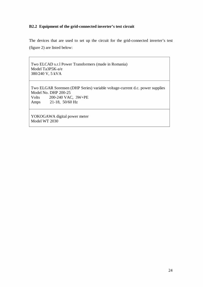
B2.2 Equipment of the grid-connected inverter’s test circuit
The devices that are used to set up the circuit for the grid-connected inverter’s test
(figure 2) are listed below:
Two ELCAD s.r.l Power Transformers (made in Romania)Model Ta3P5K-a/e380/240 V, 5 kVA
Two ELGAR Sorensen (DHP Series) variable voltage-current d.c. power suppliesModel No. DHP 200-25Volts 200-240 VAC, 3W+PEAmps 21-18, 50/60 Hz
YOKOGAWA digital power meterModel WT 2030

25
Figure 3- Inverter’s test circuit. Center for Renewable Energy Sources in Greece Department of Photovoltaic Systems
Figure 4- Resistive & Reactive Loads of the test circuits. Center for Renewable Energy Sources in Greece Department of Photovoltaic Systems
Resistive LoadReactive Load

26
B2.3 Measurement procedure
a) Efficiency is calculated with equation (1) or (2) –see pages 19 & 20
respectively-, using measured Pi, Po or Pip, Pop. DC input power Pi, Pip can be
measured by digital power meter or determined by multiplying the inverter’s
input voltage and the inverter’s input current, both measured by digital power
meter. Output power Po, Pop is measured by digital power meter as well.
b) DC input voltage, which is measured by digital power meter, will be varied in
the defined range where the output current, which is also measured with digital
power meter, is varied from low output to the rated output.
c) Power factor (PF in per cent) can be measured by the digital power meter.
d) The inverter’s output current and the inveretr’s output voltage will be measured
by the the digital power meter as well as the THD of current and the THD of
voltage.
e) Based on the graph of the output current, which is shown at the monitor of the
oscilloscope, we can evaluate each time, the current ripple of the inverter’s
output current.
f) In case of grid-connected inverter, we further measure the harmonics of voltage
and the harmonics of current injected into grid, by using the digital power
meter, shown in figure 2, page 21.
Loss measurement
No-load loss will be measured as follows.
• If the inverter is a stand-alone type, the reading of d.c. input voltage, output
voltage and frequency is given with digital power meter and will be adjusted to
the rated values.
No-load loss is thus the indicated value of d.c. input power measured by power
meter in figure 1, page 21, when the load is disconnected from the inverter.
• If the inverter is a utility-interactive type, the reading of d.c. input voltage, a.c.
output voltage and frequency is given with digital power meter and will be
agjusted to meet the specified voltages and frequency.
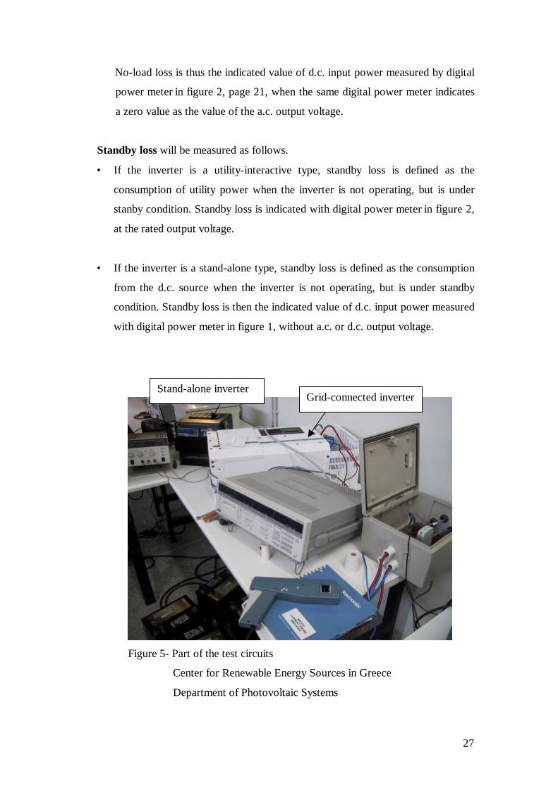
27
No-load loss is thus the indicated value of d.c. input power measured by digital
power meter in figure 2, page 21, when the same digital power meter indicates
a zero value as the value of the a.c. output voltage.
Standby loss will be measured as follows.
• If the inverter is a utility-interactive type, standby loss is defined as the
consumption of utility power when the inverter is not operating, but is under
stanby condition. Standby loss is indicated with digital power meter in figure 2,
at the rated output voltage.
• If the inverter is a stand-alone type, standby loss is defined as the consumption
from the d.c. source when the inverter is not operating, but is under standby
condition. Standby loss is then the indicated value of d.c. input power measured
with digital power meter in figure 1, without a.c. or d.c. output voltage.
Figure 5- Part of the test circuits
Center for Renewable Energy Sources in Greece
Department of Photovoltaic Systems
Stand-alone inverterGrid-connected inverter
28
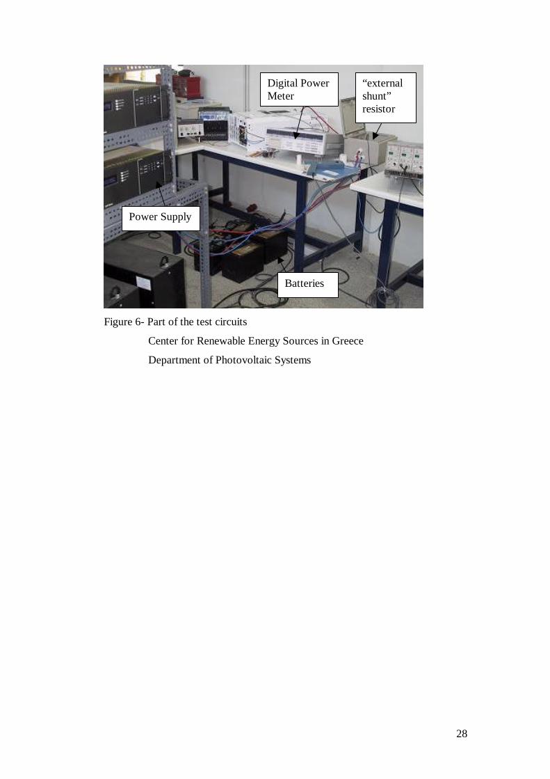
Figure 6- Part of the test circuits
Center for Renewable Energy Sources in Greece
Department of Photovoltaic Systems
Digital PowerMeter
Batteries
“externalshunt”resistor
Power Supply

29
C. INVERTERS, WHICH ARE TESTED
C1. STAND-ALONE TYPE
Trace Engineering inverter (made in U.S.A.)
Model 2524
2,5 kW
Nominal Input Voltage 24 VDC
Input Voltage Range 14,9 V - 30,7 V
Nominal output Range 220 VAC
50 Hz
The above model of Trace Engineering stand-alone inverter belongs to Trace 2500
series Inverters, which are modified square wave inverters.
The topology of this series of inverters is named push-pull topology and it’s based on
low frequency switching of the low voltage DC side, applying the resulting DC pulses
to a step-up transformer.
Design and operation of the inverter
The basic theory of operation behind a push-pull design is as follows:
The top transistor switch closes and causes current to flow from the battery negative
thriugh the transformer primary to the battery positive. This induces a voltage in the
secondary side of the transformer that is equal to the battery voltage times the turns
ratio of the transformer. Note: Only one switch at a time is closed.
After a period of approximately 8ms (one-half of a 60 Hz AC cycle), the switches flip-
flop. The top switch opens and then the bottom switch closes allowing current to flow
in the opposite direction. This cycle continues and higher voltage AC power is the
result.

30
The above type of operation produces a square wave result. The addition of an extra
winding in the transformer along with a few other parts allows output of a modified
square wave.
So, at modified square wave inverters, as the model 2524 of Trace Engineering, the
switching cycle is identical to that described above, except for one additional step. In
the switching cycle, another step is added, which “clears” out the transformer reducing
the problems associated with the sudden change in current direction. This is
accomplished by the off time shorting winding shown in figure 7. As one switch opens
and before the second switch closes, the switch across the shorting winding closes,
effectively removing the current from the transformer. Off-time shorting provides a
better zero crossing of the waveform, which equates to better ability to operate
electronic devices. Improved efficiency is another one benefit.
Figure 7- Push-pull topology with shorting winding

31
C2. GRID-CONNECTED TYPE
Total Energie inverter (made in France)
Model Onbuleur Joule Prg
2,5 kW
Single phase
Nominal Input Voltage 48 VDC
Input Voltage Range 44 V - 66 V
Nominal output Range 220 VAC
50 Hz
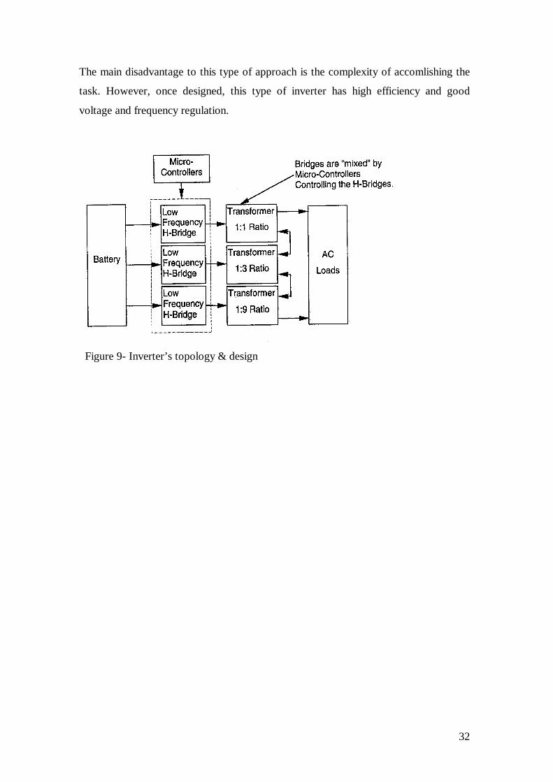
Total Energie inverter is based on the Trace Engineering SW series, which uses a
combination of three transformers, each with its own low frequency switcher, coupled
together in series and driven by separate interconnected micro-controllers. In essence it
is three inverters linked together by their transformers. By mixing the outputs from the
different transformers, a stepped approximation of a sine wave is produced. Shown
in figure 8 is the output waveform from this kind of inverter. Notice the “steps” form a
staircase that is shaped like a sine wave.
Figure 8- Output of the above type of grid-connected inverter
The multi-stepped output is formed by modulation of the voltage through mixing of the
three transformers in a specific order. Anywhere from 34-52 “steps” per AC cycle may
be present in the waveform. The heavier the load or lower DC input voltage the more
steps there are in the waveform.
32
The main disadvantage to this type of approach is the complexity of accomlishing the
task. However, once designed, this type of inverter has high efficiency and good
voltage and frequency regulation.
Figure 9- Inverter’s topology & design
33
Chapter 3
RESULTS & CONCLUSIONS
A. STAND-ALONE INVERTER’S TEST RESULTS
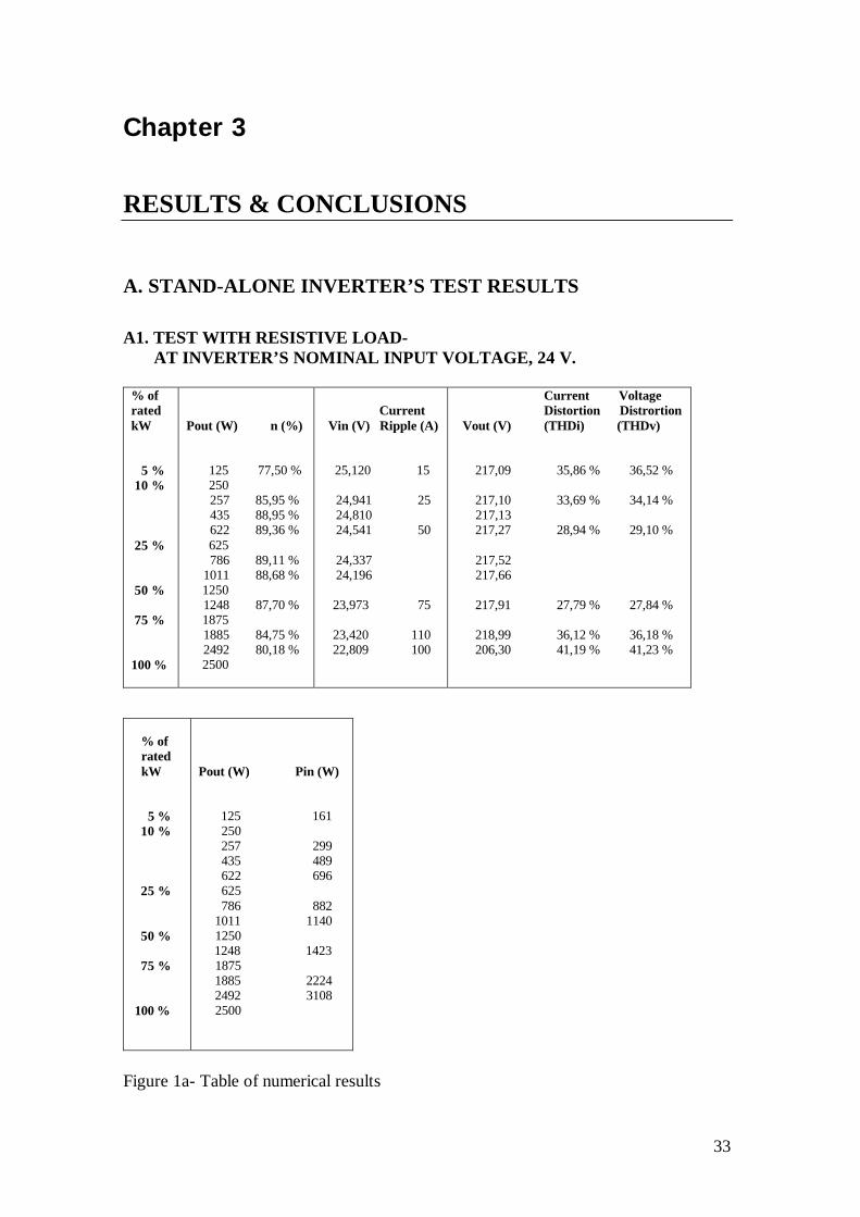
A1. TEST WITH RESISTIVE LOAD- AT INVERTER’S NOMINAL INPUT VOLTAGE, 24 V.
% ofratedkW
5 % 10 %
25 %
50 %
75 %
100 %
Pout (W) n (%)
125 77,50 %250257 85,95 %435 88,95 %622 89,36 %625786 89,11 %
1011 88,68 %12501248 87,70 %18751885 84,75 %2492 80,18 %2500
CurrentVin (V) Ripple (A)
25,120 15
24,941 2524,81024,541 50
24,33724,196
23,973 75
23,420 11022,809 100
Current Voltage Distortion Distrortion Vout (V) (THDi) (THDv)
217,09 35,86 % 36,52 %
217,10 33,69 % 34,14 % 217,13 217,27 28,94 % 29,10 %
217,52 217,66
217,91 27,79 % 27,84 %
218,99 36,12 % 36,18 % 206,30 41,19 % 41,23 %
% of rated kW
5 % 10 %
25 %
50 %
75 %
100 %
Pout (W) Pin (W)
125 161 250 257 299 435 489
622 696625
786 882 1011 1140 1250
1248 1423 1875 1885 2224 2492 3108 2500
Figure 1a- Table of numerical results
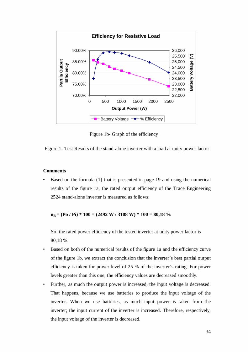
34
Efficiency for Resistive Load
70.00%
75.00%
80.00%
85.00%
90.00%
0 500 1000 1500 2000 2500
Output Power (W)
Par
tila
Out
put
Eff
icie
ncy
22,00022,50023,00023,50024,00024,50025,00025,50026,000
Bat
tery
Vol
tage
(V)
Battery Voltage % Efficiency
Figure 1b- Graph of the efficiency
Figure 1- Test Results of the stand-alone inverter with a load at unity power factor
Comments
• Based on the formula (1) that is presented in page 19 and using the numerical
results of the figure 1a, the rated output efficiency of the Trace Engineering
2524 stand-alone inverter is measured as follows:
nR = (Po / Pi) * 100 = (2492 W / 3108 W) * 100 = 80,18 %
So, the rated power efficiency of the tested inverter at unity power factor is
80,18 %.
• Based on both of the numerical results of the figure 1a and the efficiency curve
of the figure 1b, we extract the conclusion that the inverter’s best partial output
efficiency is taken for power level of 25 % of the inverter’s rating. For power
levels greater than this one, the efficiency values are decreased smoothly.
• Further, as much the output power is increased, the input voltage is decreased.
That happens, because we use batteries to produce the input voltage of the
inverter. When we use batteries, as much input power is taken from the
inverter; the input current of the inverter is increased. Therefore, respectively,
the input voltage of the inverter is decreased.

35
• In general, based on the results presented in figure 1a and 1b, we can say that
the efficiency of the inverter as well as its whole behaviour at unity power
factor (resistive load, cosϕ = 1) is very good.

36
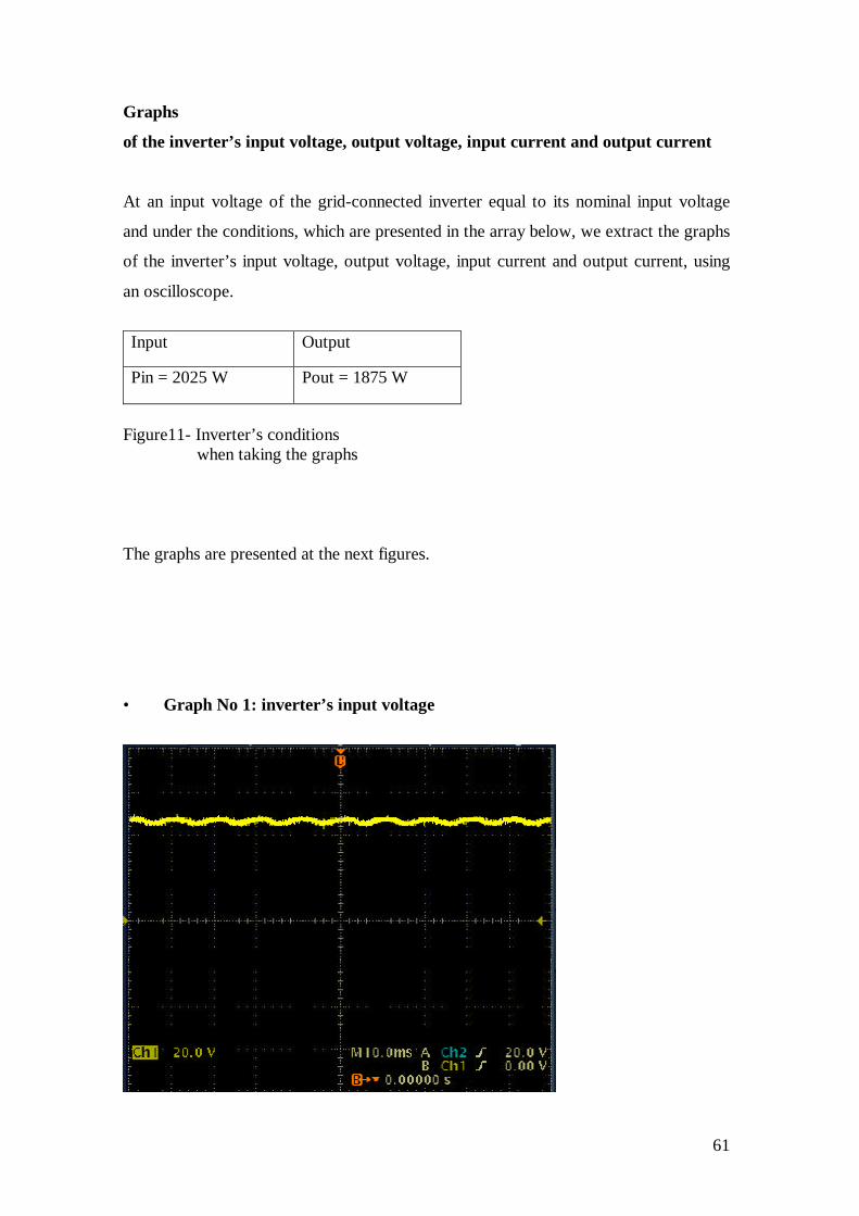
Graphs
of the inverter’s input voltage, output voltage, input current and output current
At unity power factor of the stand-alone inverter and under the conditions, which are
presented in the array below, we extract the graphs of the inverter’s input voltage,
output voltage, input current and output current, using an oscilloscope.
Input Output
Pin = 943 W Pout = 884 W
Figure 2- Inverter’s conditions when taking the graphs
The graphs are presented at the next figures.
• Graph No 1: inverter’s input voltage
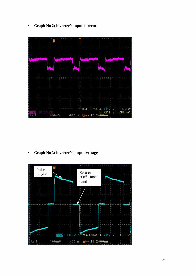
37
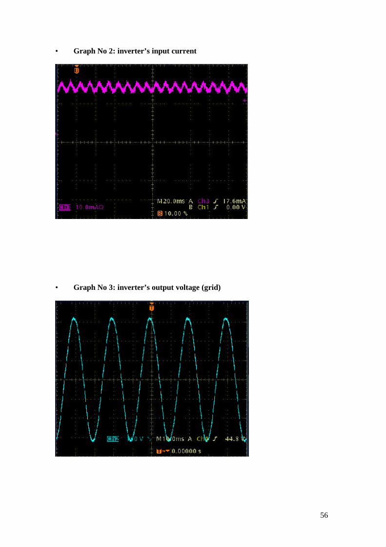
• Graph No 2: inverter’s input current
• Graph No 3: inverter’s output voltage
Zero or“Off Time”band
Pulseheight

38
• Graph No 4: inverter’s output current
Comments
The output voltage of the Trace Engineering 2524 stand-alone inverter (graph No 3)
shows that its output is a modified square wave (often referred to as modified sine
wave). The graph of the output voltage is similar to the graph in figure 2, page 8,
which according to the theory represents the output of a modified square wave inverter.
The zero or “Off Time” band and pulse height have been shown with arrows up to the
graph.
The next graphs (graph No 5 and graph No 6) show the inverter’s input voltage and
current together, as well as the inverter’s output voltage and current together.

39
• Graph No 5: inverter’s input current and voltage
• Graph No 6: inverter’s output current and voltage
40
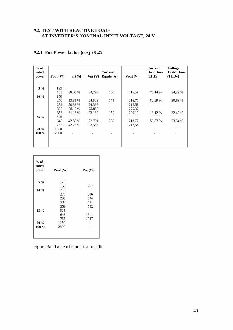
A2. TEST WITH REACTIVE LOAD- AT INVERTER’S NOMINAL INPUT VOLTAGE, 24 V.
A2.1 For Power factor (cosϕ) 0,25
% ofratedpower
5 %
10 %
25 %
50 %100 %
Pout (W) n (%)
125155 58,05 %250270 53,35 %299 50,33 %337 78,19 %356 61,16 %625648 42,88 %755 42,25 %
1250 -2500 -
Current Vin (V) Ripple (A)
24,797 100
24,503 17524,398
22,88923,180 150
23.791 23023,565
- - - -
Current Voltage Distortion Distrortion Vout (V) (THDi) (THDv)
216,59 75,14 % 34,39 %
216,71 82,29 % 30,68 % 216,58 220,32 220,19 13,12 % 32,49 %
218,72 59,87 % 23,54 % 218,58 - - - - - -
% ofratedpower
5 %
10 %
25 %
50 %100 %
Pout (W) Pin (W)
125155 267250270 506299 594337 431356 582625648 1511755 1787
1250 -2500 -
Figure 3a- Table of numerical results
41
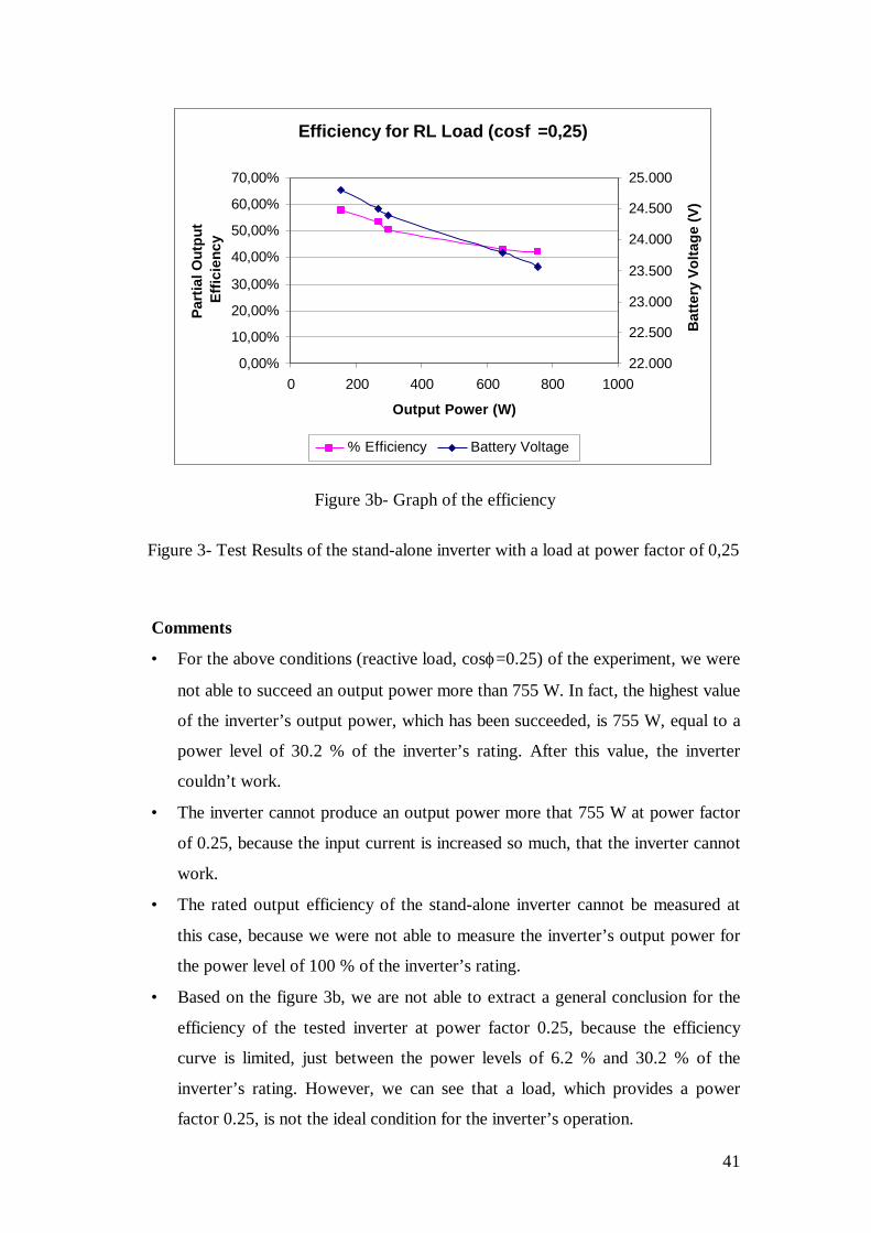
Efficiency for RL Load (cosf =0,25)
0,00%
10,00%
20,00%
30,00%
40,00%
50,00%
60,00%
70,00%
0 200 400 600 800 1000
Output Power (W)
Par
tial O
utpu
t E
ffic
ienc
y
22.000
22.500
23.000
23.500
24.000
24.500
25.000
Bat
tery
Vol
tage
(V)
% Efficiency Battery Voltage
Figure 3b- Graph of the efficiency
Figure 3- Test Results of the stand-alone inverter with a load at power factor of 0,25
Comments
• For the above conditions (reactive load, cosϕ=0.25) of the experiment, we were
not able to succeed an output power more than 755 W. In fact, the highest value
of the inverter’s output power, which has been succeeded, is 755 W, equal to a
power level of 30.2 % of the inverter’s rating. After this value, the inverter
couldn’t work.
• The inverter cannot produce an output power more that 755 W at power factor
of 0.25, because the input current is increased so much, that the inverter cannot
work.
• The rated output efficiency of the stand-alone inverter cannot be measured at
this case, because we were not able to measure the inverter’s output power for
the power level of 100 % of the inverter’s rating.
• Based on the figure 3b, we are not able to extract a general conclusion for the
efficiency of the tested inverter at power factor 0.25, because the efficiency
curve is limited, just between the power levels of 6.2 % and 30.2 % of the
inverter’s rating. However, we can see that a load, which provides a power
factor 0.25, is not the ideal condition for the inverter’s operation.

42
A2.2 For Power factor (cosϕ) 0,50
% ofratedpower
10 %
25 %
50 %
75 %100 %
Pout (W) n (%)
250263 74,08 %399 73,34 %503 71,04 %619 70,82 %625777 69,93 %
1086 63,80 %1250 63,22 % 1485 63,00 % 1606 63,35 %1875 -2500 -
Current Vin (V) Ripple (A)
24,518 7524,32224,15124,005 175
23,824 16023,392 200
23,225 24022,962 250
22,926 225 - -
- -
Current Voltage Distortion Distrortion Vout (V) (THDi) (THDv)
217,18 54,37 % 31,81 % 217,41 217,85 218,13 37,05 % 27,22 %
219,07 22,66 % 29,89 % 219,43 48,48 % 31,86 % 219,40 56,03 % 34,75 % 213,51 53,34 % 35,50 % 210,76 47,74 % 38,64 % - - - - - -
% ofratedpower
10 %
25 %
50 %100 %
Pout (W) Pin (W)
250263 355399 544503 708619 874625777 1111
1086 17021250 1977 1485 2357 1606 25351875 -
2500 -
Figure 4a- Table of numerical results
43
Efficiency for RL Load (cosf =0,50)
0,00%10,00%20,00%30,00%40,00%50,00%60,00%70,00%80,00%90,00%
100,00%
0 500 1000 1500 2000 2500
Output Power (W)
Par
tial o
utpu
t Eff
icie
ncy
22.000
22.500
23.000
23.500
24.000
24.500
25.000
Bat
tery
Vol
tage
(V)
% Efficiency Battery Voltage
Figure 4b- Graph of the efficiency
Figure 4- Test Results of the stand-alone inverter with a load at power factor of 0,50
Comments
• As in the previous case of the load, which provides a power factor 0.25, here,
where the load provides a power factor 0.50, we are not able to succeed an
output power of the stand-alone inverter, equal to the inverter’s rating power.
Therefore, we are not able to measure the rated output efficiency of the Trace
Engineering 2524 stand-alone inverter, at power factor 0.50.
• The highest value of the inverter’s output power, which has been succeeded
during our measurements, was 1606 W, equal to a power level of 64.24 % of
the inverter’s rating.
• The reason that the stand-alone inverter cannot produce an output power more
than 1606 W is here the same, as in measurements with a load, which provides
a power factor of 0.25. After the value of 1606 W, the input current was so
high, that the inverter couldn’t work. However, at the present measurements,
we were able to extract a higher value of the output power than before. That
happens because now, the power factor has been increased at the value of 0.50.
• The figure 4b shows that when the output power of the inverter is increased,
then the voltage of the batteries is decreased. That is rational, because when the

44
inverter’s input power is increased, the input d.c curent of the inverter is
increased as well. So, consequently, the inverter’s input voltage is decreased.
• Figure 4b shows that while the inverter’s efficiency begins at a high value, after
it is decreased step by step. Namely, the highest partial efficiency value, which
has been measured is 74,08 %, which is not of course an ideal value for the
stand-alone inverter.
45
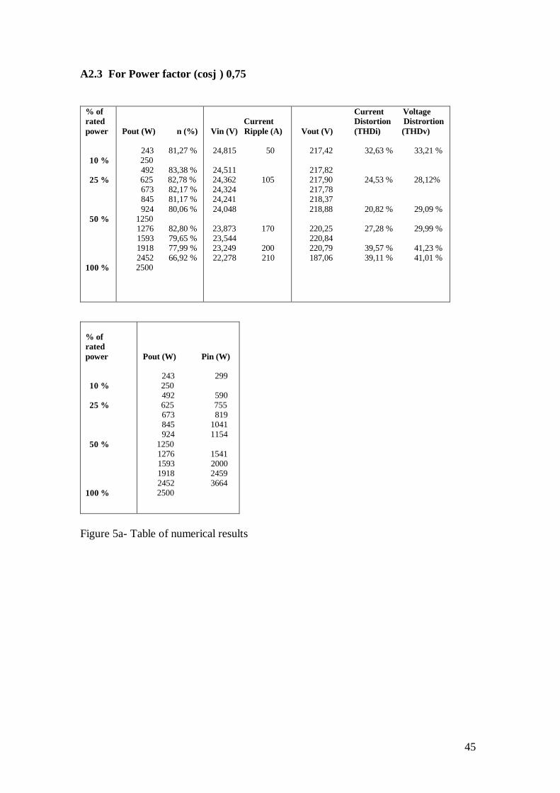
A2.3 For Power factor (cosϕ) 0,75
% ofratedpower
10 %
25 %
50 %
100 %
Pout (W) n (%)
243 81,27 %250492 83,38 %625 82,78 %673 82,17 %845 81,17 %924 80,06 %
12501276 82,80 %
1593 79,65 %1918 77,99 %2452 66,92 %2500
Current Vin (V) Ripple (A)
24,815 50
24,51124,362 10524,32424,241
24,048
23,873 170 23,54423,249 200
22,278 210
Current Voltage Distortion Distrortion Vout (V) (THDi) (THDv)
217,42 32,63 % 33,21 %
217,82 217,90 24,53 % 28,12% 217,78 218,37 218,88 20,82 % 29,09 %
220,25 27,28 % 29,99 % 220,84 220,79 39,57 % 41,23 % 187,06 39,11 % 41,01 %
% ofratedpower
10 %
25 %
50 %
100 %
Pout (W) Pin (W)
243 299250492 590625 755673 819845 1041924 1154
12501276 1541
1593 20001918 24592452 3664
2500
Figure 5a- Table of numerical results

46
Efficiency for RL Load (cosf =0,75)
0,00%10,00%20,00%30,00%40,00%50,00%60,00%70,00%80,00%90,00%
100,00%
0 500 1000 1500 2000 2500
Output Power (W)
Par
tial O
utpu
t E
ffic
ienc
y
22.000
22.500
23.000
23.500
24.000
24.500
25.000
Bat
tery
Vol
tage
(V)
% Efficiency Battery Voltage
Figure 5b- Graph of the efficiency
Figure 5- Test Results of the stand-alone inverter with a load at power factor of 0,75
Comments
• Based on the formula (1) that is presented in page 19 and using the numerical
results of the figure 1a, the rated output efficiency of the Trace Engineering
2524 stand-alone inverter is measured as follows:
nR = (Po / Pi) * 100 = (2452 W / 3664 W) * 100 = 66,92 %
So, the rated power efficiency of the tested inverter at power factor 0.75 is
66,92 %. This value is not of course the best that a modified stand-alone inverter
can produce.
• The highest partial efficiency, which is measured is 83,38 %. This value is
derived for an output power 492 W, equal to a power level of 19,68 % of the
inverter’s rating. After this value, the efficiency is decreased.
• The efficiency curve in figure 5b is not very smooth and of course in any case
is not linear. The inverter’s behaviour seems not to satisfy us completely.
47
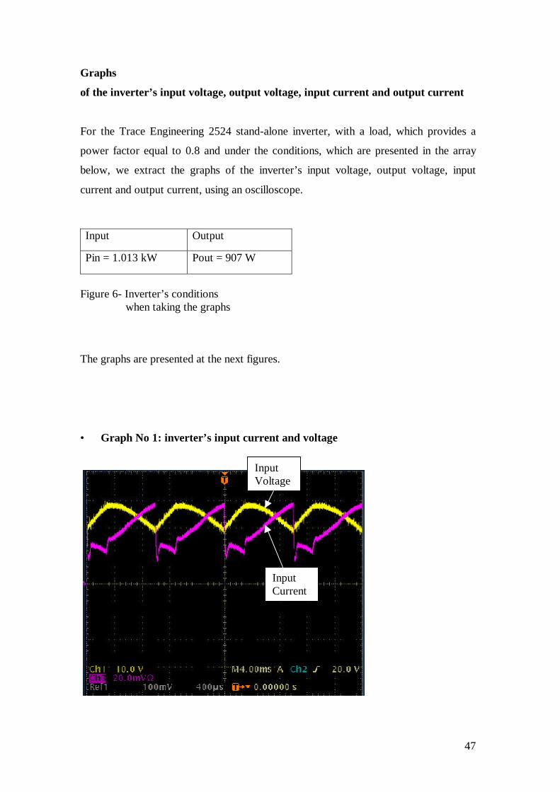
Graphs
of the inverter’s input voltage, output voltage, input current and output current
For the Trace Engineering 2524 stand-alone inverter, with a load, which provides a
power factor equal to 0.8 and under the conditions, which are presented in the array
below, we extract the graphs of the inverter’s input voltage, output voltage, input
current and output current, using an oscilloscope.
Input Output
Pin = 1.013 kW Pout = 907 W
Figure 6- Inverter’s conditions when taking the graphs
The graphs are presented at the next figures.
• Graph No 1: inverter’s input current and voltage
InputVoltage
InputCurrent

48
• Graph No 2: inverter’s output current and voltage
OutputVoltage
OutputCurrent
49
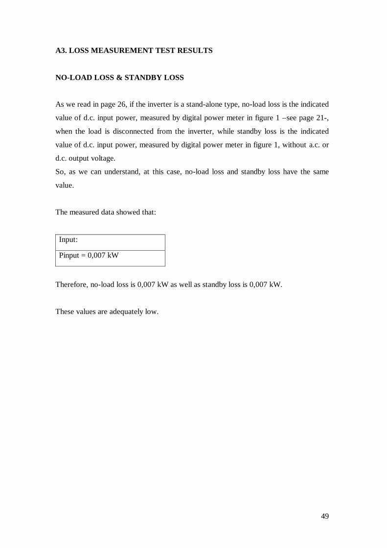
A3. LOSS MEASUREMENT TEST RESULTS
NO-LOAD LOSS & STANDBY LOSS
As we read in page 26, if the inverter is a stand-alone type, no-load loss is the indicated
value of d.c. input power, measured by digital power meter in figure 1 –see page 21-,
when the load is disconnected from the inverter, while standby loss is the indicated
value of d.c. input power, measured by digital power meter in figure 1, without a.c. or
d.c. output voltage.
So, as we can understand, at this case, no-load loss and standby loss have the same
value.
The measured data showed that:
Input:
Pinput = 0,007 kW
Therefore, no-load loss is 0,007 kW as well as standby loss is 0,007 kW.
These values are adequately low.
50
A4. CONCLUSIONS
Efficiency for RL Loads
20.00%
30.00%
40.00%
50.00%
60.00%
70.00%
80.00%
90.00%
100.00%
0 400 800 1200 1600 2000 2400
Output Power (W)
Par
tial O
utpu
t Eff
icie
ncy
cosf =0,25
cosf =0,50
cosf =0,75
cosf =1
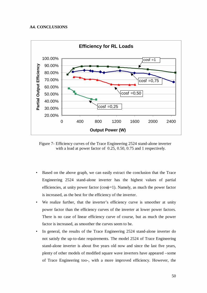
Figure 7- Efficiency curves of the Trace Engineering 2524 stand-alone inverter with a load at power factor of 0.25, 0.50, 0.75 and 1 respectively.
• Based on the above graph, we can easily extract the conclusion that the Trace
Engineering 2524 stand-alone inverter has the highest values of partial
efficiencies, at unity power factor (cosϕ=1). Namely, as much the power factor
is increased, as the best for the efficiency of the inverter.
• We realize further, that the inverter’s efficiency curve is smoother at unity
power factor than the efficiency curves of the inverter at lower power factors.
There is no case of linear efficiency curve of course, but as much the power
factor is increased, as smoother the curves seem to be.
• In general, the results of the Trace Engineering 2524 stand-alone inverter do
not satisfy the up-to-date requirements. The model 2524 of Trace Engineering
stand-alone inverter is about five years old now and since the last five years,
plenty of other models of modified square wave inverters have appeared –some
of Trace Engineering too-, with a more improved efficiency. However, the

51
opinion that the modified square wave inverters are suitable for resistive loads,
which has been written in the introduction of this paper –see page 8, Chapter 1-
is verified here, by the results of our experiment.
52
B. GRID-CONNECTED INVERTER’S TEST RESULTS
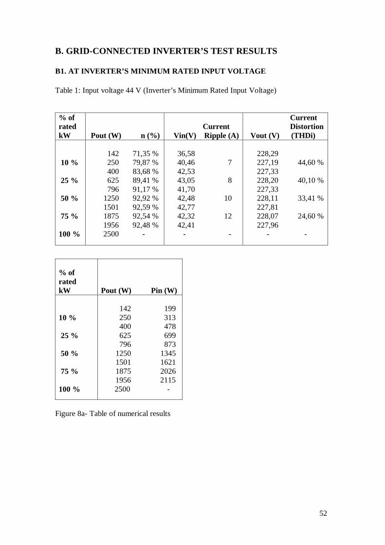
B1. AT INVERTER’S MINIMUM RATED INPUT VOLTAGE
Table 1: Input voltage 44 V (Inverter’s Minimum Rated Input Voltage)
% ofratedkW Pout (W) n (%)
Current Vin(V) Ripple (A)
CurrentDistortion
Vout (V) (THDi)
10 %
25 %
50 %
75 %
100 %
142 71,35 % 250 79,87 % 400 83,68 % 625 89,41 % 796 91,17 %
1250 92,92 % 1501 92,59 % 1875 92,54 %
1956 92,48 %2500 -
36,58 40,46 7 42,53 43,05 8 41,70 42,48 10 42,77 42,32 12 42,41 - -
228,29227,19 44,60 %227,33228,20 40,10 %227,33228,11 33,41 %227,81228,07 24,60 %227,96 - -
% ofratedkW Pout (W) Pin (W)
10 %
25 %
50 %
75 %
100 %
142 199 250 313 400 478 625 699 796 873
1250 1345 1501 1621 1875 2026
1956 2115 2500 -
Figure 8a- Table of numerical results

53
Figure 8b- Efficiency curve
Figure 8c- Graph of THDi vs Power Output
Figure 8- Test Results of the grid-connected inverter at input voltage 44 V
Efficiency Curve
50%
60%
70%
80%
90%
100%
0 500 1000 1500 2000 2500 3000
Output Power (W)
Par
tial O
utpu
t Eff
icie
ncy
THD Current vs Power Output
0.00%
10.00%
20.00%
30.00%
40.00%
50.00%
0 500 1000 1500 2000
Power Output (W)
TH
D C
urre
nt

54
Comments
• Based on both of the numerical results of the figure 8a and the efficiency curve
of the figure 8b, we extract the conclusion that the inverter’s best partial output
efficiency has been derived for power level of 50 % of the inverter’s rating.
However, for power levels greater than 50 %, the values of the partial output
efficiency are not so much different. In general, the efficiency of the grid-
connected inverter, for power levels greater than 50 % of the inverter’s rating,
remains at the same almost values. That is a very important characteristic of the
inverter, because after it succeeds an output power equal to 1250 W, it follows
an almost constant performance.
• In order to produce an inverter’s input voltage equal to 44 V, we used two
power supplies, as it is shown in figure 2 of the second chapter, (see page 21).
The power supplies were manually programmable. So, each time, the power
supplies were programmed to provide an output voltage of 44 V, equal to the
inverter’s input voltage. However, as we can see in figure 8a, the power
supplies were not able to provide a total output voltage equal to 44 V. So, the
input voltage of the grid-connected inverter was increasing, only when the
output power of the inverter was increasing as well. Namely, at this part of the
experiment, the power supplies were able to provide a final maximum output
voltage, equal to 42,41 V.
• After the value of 42,41 V, the power supplies couldn’t work. So, the rated
output efficiency of the grid-connected inverter could not be measured at this
case, as we were not able to measure the inverter’s output power for the power
level of 100 % of the inverter’s rating.
• The distortion of the output current (THDi) is decreased as the output power
and the partial output efficiency of the grid-connected inverter are increased.
55
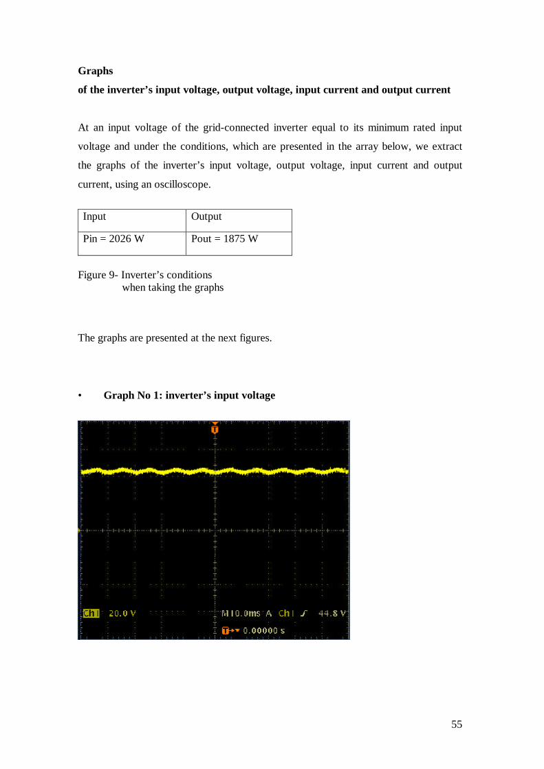
Graphs
of the inverter’s input voltage, output voltage, input current and output current
At an input voltage of the grid-connected inverter equal to its minimum rated input
voltage and under the conditions, which are presented in the array below, we extract
the graphs of the inverter’s input voltage, output voltage, input current and output
current, using an oscilloscope.
Input Output
Pin = 2026 W Pout = 1875 W
Figure 9- Inverter’s conditions when taking the graphs
The graphs are presented at the next figures.
• Graph No 1: inverter’s input voltage
56
• Graph No 2: inverter’s input current
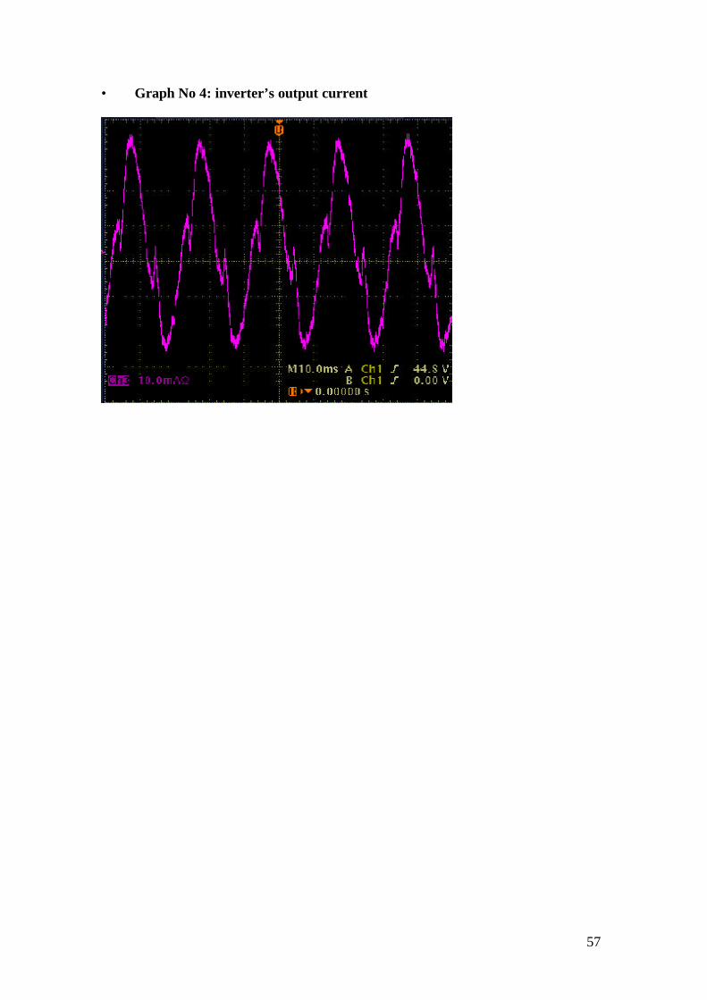
• Graph No 3: inverter’s output voltage (grid)
57
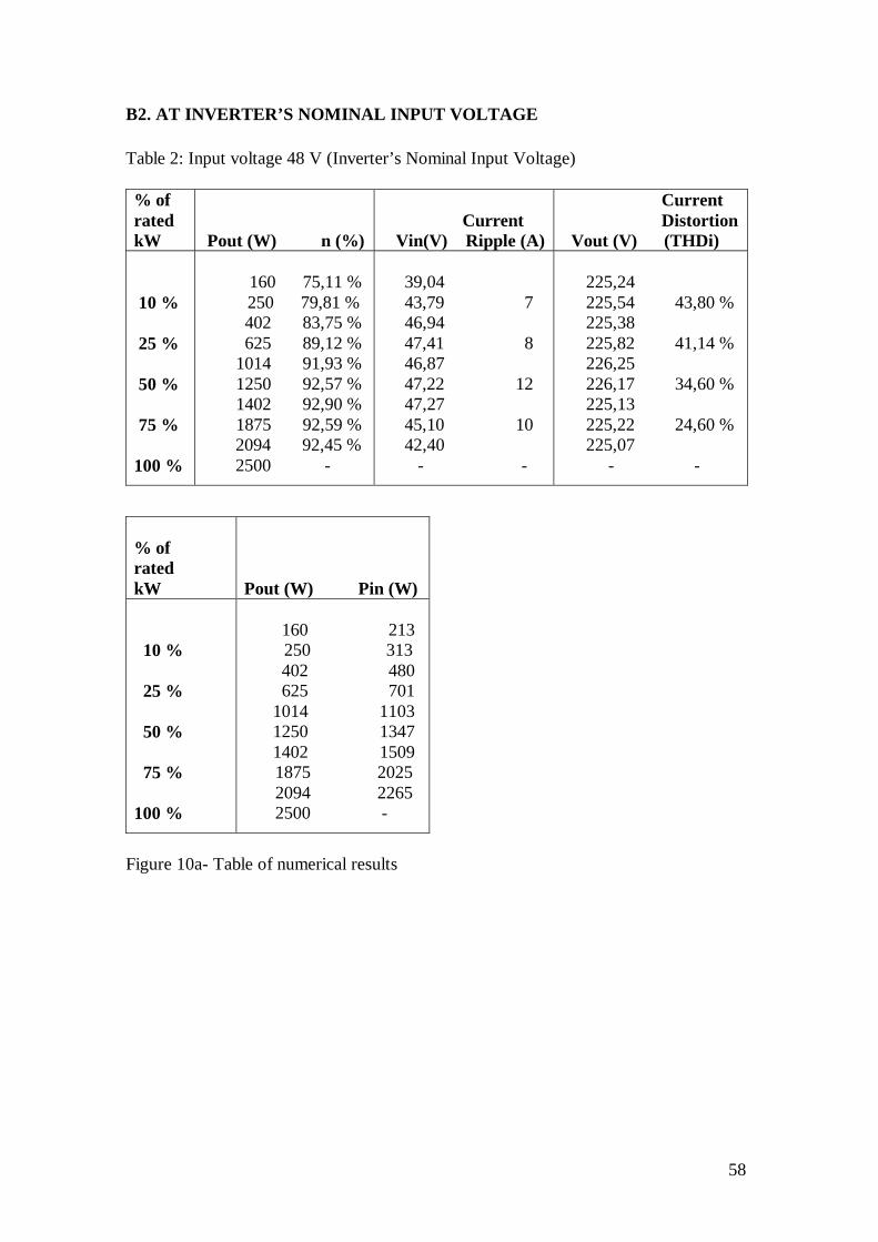
• Graph No 4: inverter’s output current
58
B2. AT INVERTER’S NOMINAL INPUT VOLTAGE
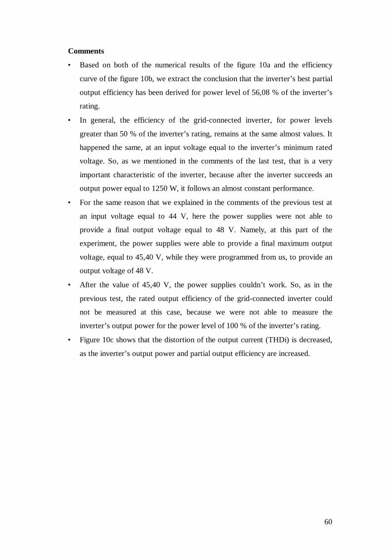
Table 2: Input voltage 48 V (Inverter’s Nominal Input Voltage)
% ofratedkW Pout (W) n (%)
Current Vin(V) Ripple (A)
CurrentDistortion
Vout (V) (THDi)
10 %
25 %
50 %
75 %
100 %
160 75,11 % 250 79,81 %
402 83,75 % 625 89,12 % 1014 91,93 %
1250 92,57 % 1402 92,90 % 1875 92,59 %
2094 92,45 %2500 -
39,04 43,79 7 46,94 47,41 8 46,87 47,22 12 47,27 45,10 10 42,40 - -
225,24225,54 43,80 %225,38225,82 41,14 %226,25226,17 34,60 %225,13225,22 24,60 %225,07 - -
% ofratedkW Pout (W) Pin (W)
10 %
25 %
50 %
75 %
100 %
160 213 250 313
402 480 625 7011014 1103
1250 1347 1402 1509
1875 2025 2094 2265 2500 -
Figure 10a- Table of numerical results

59
Figure 10b- Efficiency curve
Figure 10c- Graph of THDi vs Power Output
Figure 10- Test Results of the grid-connected inverter at input voltage 48 V
Efficiency Curve
50%
60%
70%
80%
90%
100%
0 500 1000 1500 2000 2500 3000
Output Power (W)
Par
tail
Out
put E
ffic
ienc
y
THD Current vs Power Output
0.00%
10.00%
20.00%
30.00%
40.00%
50.00%
0 500 1000 1500 2000Power Output (W)
TH
D C
urre
nt
60
Comments
• Based on both of the numerical results of the figure 10a and the efficiency
curve of the figure 10b, we extract the conclusion that the inverter’s best partial
output efficiency has been derived for power level of 56,08 % of the inverter’s
rating.
• In general, the efficiency of the grid-connected inverter, for power levels
greater than 50 % of the inverter’s rating, remains at the same almost values. It
happened the same, at an input voltage equal to the inverter’s minimum rated
voltage. So, as we mentioned in the comments of the last test, that is a very
important characteristic of the inverter, because after the inverter succeeds an
output power equal to 1250 W, it follows an almost constant performance.
• For the same reason that we explained in the comments of the previous test at
an input voltage equal to 44 V, here the power supplies were not able to
provide a final output voltage equal to 48 V. Namely, at this part of the
experiment, the power supplies were able to provide a final maximum output
voltage, equal to 45,40 V, while they were programmed from us, to provide an
output voltage of 48 V.
• After the value of 45,40 V, the power supplies couldn’t work. So, as in the
previous test, the rated output efficiency of the grid-connected inverter could
not be measured at this case, because we were not able to measure the
inverter’s output power for the power level of 100 % of the inverter’s rating.
• Figure 10c shows that the distortion of the output current (THDi) is decreased,
as the inverter’s output power and partial output efficiency are increased.
61
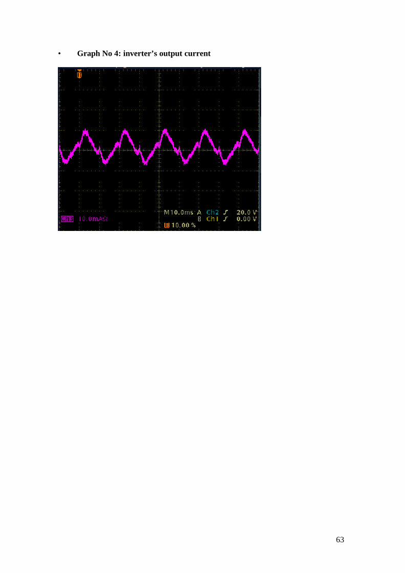
Graphs
of the inverter’s input voltage, output voltage, input current and output current
At an input voltage of the grid-connected inverter equal to its nominal input voltage
and under the conditions, which are presented in the array below, we extract the graphs
of the inverter’s input voltage, output voltage, input current and output current, using
an oscilloscope.
Input Output
Pin = 2025 W Pout = 1875 W
Figure11- Inverter’s conditions when taking the graphs
The graphs are presented at the next figures.
• Graph No 1: inverter’s input voltage

62
• Graph No 2: inverter’s input current
• Graph No 3: inverter’s output voltage (grid)
63
• Graph No 4: inverter’s output current
64
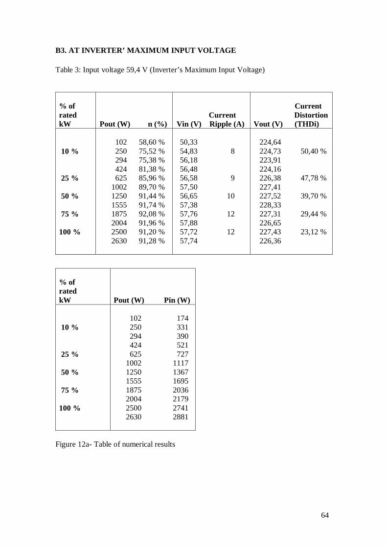
B3. AT INVERTER’ MAXIMUM INPUT VOLTAGE
Table 3: Input voltage 59,4 V (Inverter’s Maximum Input Voltage)
% ofratedkW Pout (W) n (%)
CurrentVin (V) Ripple (A)
Current Distortion
Vout (V) (THDi)
10 %
25 %
50 %
75 %
100 %
102 58,60 %250 75,52 %294 75,38 %424 81,38 %625 85,96 %
1002 89,70 %1250 91,44 %1555 91,74 %1875 92,08 %2004 91,96 %2500 91,20 %2630 91,28 %
50,3354,83 856,1856,4856,58 957,5056,65 1057,3857,76 1257,8857,72 1257,74
224,64 224,73 50,40 % 223,91 224,16 226,38 47,78 % 227,41 227,52 39,70 % 228,33 227,31 29,44 % 226,65 227,43 23,12 % 226,36
% ofratedkW Pout (W) Pin (W)
10 %
25 %
50 %
75 %
100 %
102 174250 331294 390424 521625 727
1002 11171250 13671555 16951875 20362004 21792500 27412630 2881
Figure 12a- Table of numerical results
65
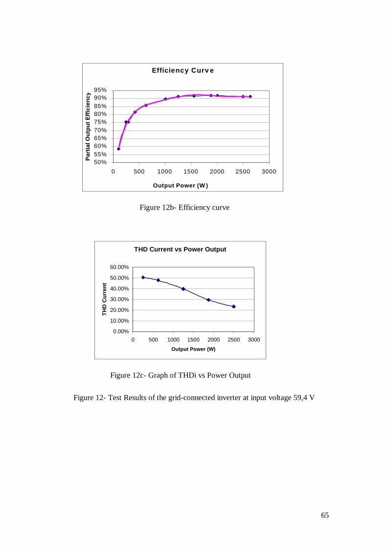
Figure 12b- Efficiency curve
Figure 12c- Graph of THDi vs Power Output
Figure 12- Test Results of the grid-connected inverter at input voltage 59,4 V
Efficiency Curv e
50%55%60%65%70%75%80%85%90%95%
0 500 1000 1500 2000 2500 3000
Output Power (W )
Par
tial O
utpu
t Eff
icie
ncy
THD Current vs Power Output
0.00%
10.00%
20.00%
30.00%
40.00%
50.00%
60.00%
0 500 1000 1500 2000 2500 3000
Output Power (W)
TH
D C
urre
nt
66
Comments
• Based on the figures 12a and 12b, we extract the conclusion that the inverter’s
best partial output efficiency has been derived for power level of 75 % of the
inverter’s rating.
• The rated output efficiency of the tested grid-connected inverter at input
voltage equal to 90 % of the inverter’s maximum input voltage, is calculated
based on the formula (1), which is presented in chapter 2, page 19, and using
the numerical results of the figure 12a, as follows:
nR = (Po / Pi) * 100 = (2500 W / 2741 W) * 100 = 91,20 %
Therefore, the rated power efficiency of the tested inverter at input voltage
equal to 59,4 V is 91,20 %.
Of course, writing that the inverter input voltage is equal to 59.4 V, we mean
that the power supplies have been programmed by us, to provide an output
voltage of 59,4 V, while actually, they were able to provide only a maximum
voltage equal to 57,74 V.
• The inverter’s partial output efficiency, after the power level of 50 % of the
inverter’s rating, remains almost the same. Namely, firstly it is increased a
little, until to succeed its maximum value at output power equal to 1875 W,
while after it is decreased, until the value of 91,28 %, at the inverter’s output
power of 2630 W.
• The distortion of the output current (THDi) has a value of 50,40 % for power
level of 10 % of the inverter’s rating, while this value is reduced at 23,12 % for
power level of 100 % of the inverter’s rating. Figure 12c shows that the current
distortion is decreased, while the output power and the partial output efficiency
of the tested grid-connected inverter are increased.

67
B4. LOSS MEASUREMENT TEST RESULTS
NO-LOAD LOSS
As we wrote in page 26, if the inverter is a grid-connected type, no-load loss is theindicated value of d.c. input power measured by digital power meter in figure 2 –seepage 21-, when the same digital power meter indicates a zero value as the value of thea.c. output voltage.
Namely, the device that we measured, showed:
Input: Output:
Pinput = 0,023 kW Poutput = 0 W
Therefore, the no-load loss is 0,023 KW.
STANDBY LOSS
If the inverter is a utility-interactive type, standby loss is also indicated with digitalpower meter in figure 2 –see page 21-, at the rated output voltage.
So, the device that we measured, showed:
Output:
Poutput = 0,039 kW
Therefore, standby loss is 0,039 KW.
The values of the no-load and standby losses are adequate low.

68
B5. HARMONICS
With an ideal inverter, the electricity supplied to the grid would consist only of the 50Hz fundamental frequency. With real inverters, the solar electricity has a certainharmonic content. However, electronic devices, which are connected to the low-voltage grid, must comply with the general regulations for harmonics.
Harmonic currents
The digital power meter, which is used in the test circuit of the grid-connected inverter,-see figure 2, page 21-, is able to provide a list of the harmonic currents of the inverter.Thus, for power level of 25 % of the inverter’s rating, we extract the results of the firstand second columns of the array below. The third column consisted of the limits forharmonic current emission (equipment input current ≤ 16 A per phase), which arebased on harmonics standard IEC 1000-3-2.
Harmonic Harmonic Limits forOrder Amplitude Harmonic Current
Figure 13- Harmonic currents for power level 25 % of the inverter’s rating.
2 0 . 4 6 3 1 . 0 8 3 1 . 5 3 6 2 . 3 4 0 . 1 2 7 0 . 4 3 5 1 . 3 6 9 1 . 1 4 6 0 . 0 8 6 0 . 3 7 0 . 6 7 4 0 . 7 7 8 0 . 0 2 3 0 . 2 3 9 0 . 3 2 2 0 . 4
1 0 0 . 0 4 2 0 . 1 8 4 1 1 0 . 4 0 6 0 . 3 3 1 2 0 . 0 1 4 0 . 1 5 3 1 3 0 . 2 6 6 0 . 2 1 1 4 0 . 0 1 9 0 . 1 3 1 1 5 0 . 2 8 2 0 . 1 5 1 6 0 . 0 1 3 0 . 1 1 5 1 7 0 . 0 6 7 0 . 1 3 2 1 8 0 . 0 0 7 0 . 1 0 2 1 9 0 . 1 1 0 . 1 1 8 2 0 0 . 0 0 7 0 . 0 9 2 2 1 0 . 1 4 2 0 . 1 0 7 2 2 0 . 0 1 6 0 . 0 8 3 2 3 0 . 0 3 6 0 . 0 9 7 2 4 0 . 0 1 0 . 0 7 6 2 5 0 . 1 5 0 . 0 9 2 6 0 . 0 1 8 0 . 0 7 2 7 0 . 0 2 8 0 . 0 8 3 2 8 0 . 0 0 6 0 . 0 6 5 2 9 0 . 0 3 3 0 . 0 7 7 3 0 0 . 0 0 2 0 . 0 6 1 3 1 0 . 0 6 0 . 0 7 2 3 2 0 . 0 0 6 0 . 0 5 7 3 3 0 . 0 5 2 0 . 0 6 8 3 4 0 . 0 1 9 0 . 0 5 4 3 5 0 . 0 4 2 0 . 0 6 4 3 6 0 . 0 1 0 . 0 5 1 3 7 0 . 0 3 4 0 . 0 6 3 8 0 . 0 0 4 0 . 0 4 8 3 9 0 . 0 4 6 0 . 0 5 7 4 0 0 . 0 2 5 0 . 0 4 6 4 1 0 . 0 7 4 2 0 . 0 1 4 3 0 . 0 1 2 4 4 0 . 0 0 8 4 5 0 . 0 2 5 4 6 0 . 0 0 2 4 7 0 . 0 2 6 4 8 0 . 0 1 6 4 9 0 . 0 4 4 5 0 0 . 0 0 2

69
Based on the array of the previous page, we draw the next graph.
Figure 14- Current Harmonics of the tested grid-connected inverter at Pac=625 W compared to limits of IEC 1000-3-2.
By the same way, we measure the harmonic currents of the Total Energieinverter, for power levels of 50 % and 84,2 % of the inverter’s rating. Theresults are represented at the next two graphs, respectively.
Harmonic Currents
0
0.5
1
1.5
2
2.5
2 7 12 17 22 27 32 37 42 47
Harmonic Order
Har
mon
ic
Am
plitu
de
0
0.5
1
1.5
2
2.5
Lim
its fo
r H
arm
onic
Cur
rent
E
mis
sion
Harmonic Amplitude Limits for Harmonic Current Emission
Figure 15- Current Harmonics of the tested grid-connected inverter at Pac=1250 W compared to limits of IEC 1000-3-2.
Harmonic Currents
0
0.5
1
1.5
2
2.52 5 8 11 14 17 20 23 26 29 32 35 38 41 44 47 50
Harmonic Order
Har
mon
ic A
mpl
itude
0
0.5
1
1.5
2
2.5
Lim
its fo
r H
arm
onic
C
urre
nt E
mis
sion
Harmonic Amplitude Limits for Harmonic Current Emission

70
Harmonic Currents
0
0.5
1
1.5
2
2.5
2 6 10 14 18 22 26 30 34 38 42 46 50
Harmonic Order
Har
mon
ic A
mpl
itude
0
0.5
1
1.5
2
2.5
Lim
its fo
r H
arm
onic
C
urre
nt E
mis
sion
Harmonic Amplitude Limits for Harmonic Current Emission
Figure 16- Current Harmonics of the tested grid-connected inverter at Pac=2105 W compared to limits of IEC 1000-3-2.
Comments
• Based on the figures 14, 15, and 16, we can see that harmoniccurrents injected into grid by the tested inverter are mostly belowthe limits of IEC 1000-3-2, (equipment input current ≤ 16 A perphase). Sometimes only, at the first harmonic components, there aresome cases where the harmonic currents are not below the limits.However, the majority of them are below the limits.
• The systems of electrical energy “filter” the harmonics of current,so, the first harmonic components are the most importantcomponents that may affect the result.
71
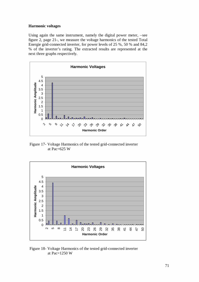
Harmonic voltages
Using again the same instrument, namely the digital power meter, –seefigure 2, page 21-, we measure the voltage harmonics of the tested TotalEnergie grid-connected inverter, for power levels of 25 %, 50 % and 84,2% of the inverter’s rating. The extracted results are represented at thenext three graphs respectively.
Harmonic Voltages
00.5
11.5
22.5
33.5
44.5
5
2 5 8 11 14 17 20 23 26 29 32 35 38 41 44 47 50
Harmonic Order
Har
mon
ic A
mpl
itude
Figure 17- Voltage Harmonics of the tested grid-connected inverter at Pac=625 W
Harmonic Voltages
00.5
11.5
22.5
33.5
44.5
5
2 5 8 11 14 17 20 23 26 29 32 35 38 41 44 47 50
Harmonic Order
Har
mon
ic A
mpl
itude
Figure 18- Voltage Harmonics of the tested grid-connected inverter at Pac=1250 W
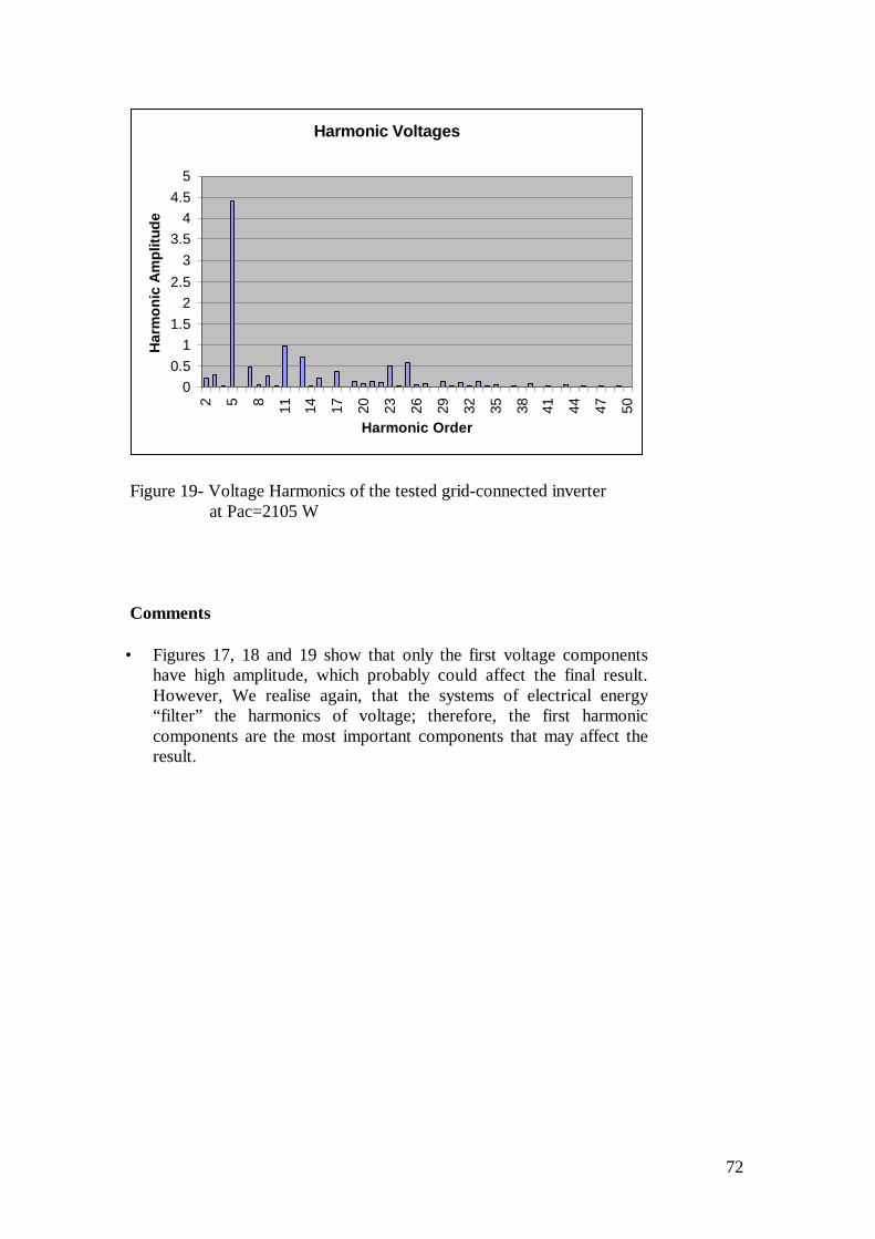
72
Harmonic Voltages
00.5
11.5
22.5
33.5
44.5
5
2 5 8 11 14 17 20 23 26 29 32 35 38 41 44 47 50
Harmonic Order
Har
mon
ic A
mpl
itude
Figure 19- Voltage Harmonics of the tested grid-connected inverter at Pac=2105 W
Comments
• Figures 17, 18 and 19 show that only the first voltage componentshave high amplitude, which probably could affect the final result.However, We realise again, that the systems of electrical energy“filter” the harmonics of voltage; therefore, the first harmoniccomponents are the most important components that may affect theresult.

73
B6. CONCLUSIONS
Figure 20- Efficiency curves of the grid-connected inverter at input voltages 44 V, 48 V and 59,4 V
• All the grid-connected inverter’s efficiency curves, which are presented at the
above figure, are smooth curves, which show that the tested inverter has a very
good performance at inverter’s input voltage equal to the inverter’s minimum
rated input voltage, to the inverter’s nominal voltage and to 90 % of the
inverter’s maximum input voltage as well. Actually, the partial efficiency
values of the inverter are higher at input voltages equal to the minimum rated
input voltage and to the inverter’s nominal voltage. At these two input voltages,
the efficiency curves are almost the same.
• For all the three above cases of the inverter’s efficiency curve, the partial
output efficiency remains each time at the same almost values, after power
level of 50 % of the inverter’s rating. It means that at every one of the three
different input voltages of the inverter, its performance remains almost
constant.
Efficiency Curve
50,00%
60,00%
70,00%
80,00%
90,00%
100,00%
0 500 1000 1500 2000 2500 3000
Output Power (W)
Par
tial O
utpu
t Eff
icie
ncy
Input Voltage=44V Input Voltage=48V Input Voltage=59,4V

74
• In general, based on the results of our experiment, we can say that the
performance of the Total Energie grid-connected inverter (Model Onbuleur
Joule Prg) is very good. It seems to satisfy the up-to-date requirements of the
customers for an inverter, which runs most of the loads, while its design, which
is based on the combination of three transformers, -see chapter 2, pages 31 &
32-, seems to be very efficient.

75
In ConclusionMany different approaches to inverter design and topology have been attempted. As
discussed, all have strong points as well as weaknesses. The “perferct” inverter has yet
to be invented, but if it were it would be 100 % efficient with infinite power and a sine
wave output. However, since nothing is free in life, we must continue to make due with
present technology and move forward, as semiconductors become batter and better.

76
Acknowledgements
The author gratefully acknowledge all the scientists of the Photovoltaic Department of
the Centre for Renewable Energy Sources in Greece for supporting the work presented
in this paper.
Namely, sincere thanks to the head of the Photovoltaic Department Dr. Christos
Protogeropoulos for offering author a place at the Power Electronics Lab of the
Photovoltaic Department and providing him all the necessary stuff.
Further, many thanks to Ioannis Nikoletatos & Aristomenis Neris for providing the
necessary theoretical background about inverters different topologies and designs and
George Panagopoulos for supporting the configuration of the experimental test
circuits of the stand-alone and grid-connected inverters.
The present project has finally carried out under the direction of the professor Dr.
Slobodan Jovanovic. Many thanks to my professor for his advise.
77
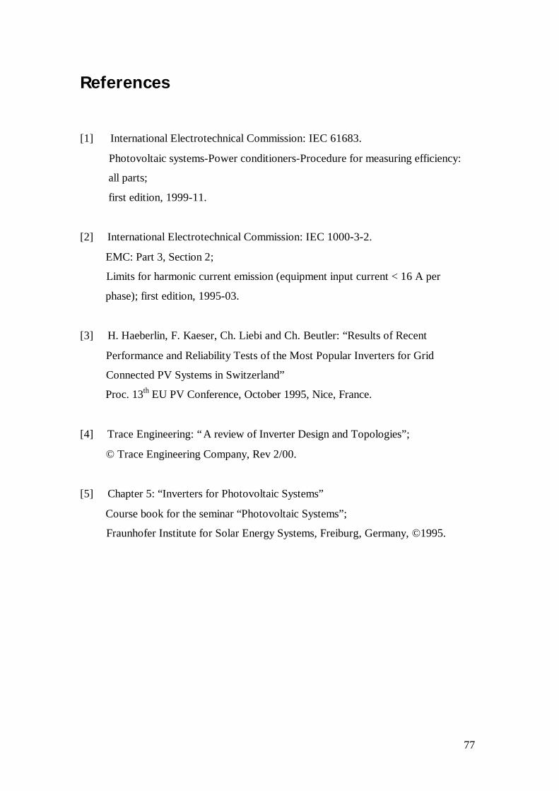
References
[1] International Electrotechnical Commission: IEC 61683.
Photovoltaic systems-Power conditioners-Procedure for measuring efficiency:
all parts;
first edition, 1999-11.
[2] International Electrotechnical Commission: IEC 1000-3-2.
EMC: Part 3, Section 2;
Limits for harmonic current emission (equipment input current < 16 A per
phase); first edition, 1995-03.
[3] H. Haeberlin, F. Kaeser, Ch. Liebi and Ch. Beutler: “Results of Recent
Performance and Reliability Tests of the Most Popular Inverters for Grid
Connected PV Systems in Switzerland”
Proc. 13th EU PV Conference, October 1995, Nice, France.
[4] Trace Engineering: “A review of Inverter Design and Topologies”;
© Trace Engineering Company, Rev 2/00.
[5] Chapter 5: “Inverters for Photovoltaic Systems”
Course book for the seminar “Photovoltaic Systems”;
Fraunhofer Institute for Solar Energy Systems, Freiburg, Germany, ©1995.