trust and information sharing in supply chainsusers.iems.northwestern.edu/~iravani/trust.pdftrust...
TRANSCRIPT

.
Trust and Information Sharing in Supply Chains
Wallace J. HoppDepartment of Industrial Engineering and Management Sciences
Northwestern University, Evanston, [email protected]
Seyed M.R. IravaniDepartment of Industrial Engineering and Management Sciences
Northwestern University, Evanston, [email protected]
Gigi Yuen-ReedIBM Global Business Services

Trust and Information Sharing in Supply Chains
Abstract
Drawing on empirical and experimental research into the composition and develop-
ment of trust, we construct a multi-period model to examine the role of trust in a supply
chain. We specifically focus on trust building in the context of a wholesale salesperson
who acts as a representative of a manufacturer and shares demand forecast information
with a retailer. The actions of the salesperson affect both her immediate economic
gain and her future credibility as determined by retailer trust. We consider three types
of salespersons: (i) a “benevolent” salesperson, whose objective is to maximize re-
tailer’s profit, (ii) a “self-serving” salesperson, whose objective is to maximize her own
quantity-based incentive pay and (iii) an “honest” salesperson who always reports her
true forecast. As we would expect, we find that a benevolent salesperson attains higher
levels of retailer trust than a self-serving salesperson. However, neither the benevolent
nor the self-serving salesperson is completely honest. A benevolent salesperson tells
occasional “white lies” (e.g., moderating an extreme forecast) to preserve trust while
a self-serving salesperson tells “manipulative lies” (e.g., inflating a forecast to drive up
order quantities). We show that increasing the length of the salesperson-retailer re-
lationship tends to induce honest behavior because of the need for the salesperson to
retain enough trust to be effective. Consequently, even a self-serving salesperson can
enable the retailer, as well as the manufacturer, to increase profits.
Keywords: Supply Chain, Trust, Lies, Relationship Building, Forecast Sharing;
1 Introduction
Since the 1990s, supply chain management has been the subject of considerable research attention.
A major concern in this research is how to coordinate the decisions of the suppliers, manufacturers
and retailers in a supply chain. Various forms of contracts and incentives have been proposed for
improving supply chain coordination and information sharing (Tsay et al. 1999 and Cachon 2003).
Recent experimental work has found that subjects tend to deviate from the optimal decisions
suggested by the contract theoretical literature (Ben-Zion et al. 2005, Bolton and Katok 2005,
Keser and Paleologo 2004, Schweitzer and Cachon 2000). This suggests that there is something
more to supply chain relationships than mere economic coordination. In this paper, we suggest
that one factor that makes up a supply chain (or indeed any business) relationship is trust.
1

Trust is important because contracts protect participating parties by specifying rights and re-
sponsibilities but they cannot address all the contingencies that may come about in today’s business
relationships (Bernheim and Whinston, 1998). Furthermore, there is overwhelming evidence on the
importance and impact of successful relationships in business decisions (Anderson and Coughlan
2002, Uzzi 1996, Zaheer and Venkatraman 1995). For example, Uzzi (1996) showed in a longitudinal
empirical study of supplier-manufacturer relations in the apparel industry that economic exchange
over time becomes rooted in complex relationships that involve economic investment, friendship
and altruistic attachments.
In collaboration with a major automotive manufacturer, we performed a field survey of the sales-
persons who represent the manufacturer to dealerships in order to understand their role in supply
chain performance (see Hopp et al. 2006 for details). Almost all of the salespersons we interviewed
indicated that the key to successful selling is a trusting and mutually beneficial relationship with
the client dealers. A key function of these salespersons is assisting the dealers in forecasting future
demand. In this paper, we specifically examine the role trust plays in this forecasting function.
Drawing on empirical and experimental research into the composition and development of trust,
we construct a multi-period model with which to examine the evolution of trust and its impact
on the sharing of demand forecast information between a salesperson and a retailer (dealer). In
each period, the retailer and the wholesale salesperson make demand forecasts. Depending on the
circumstances, the salesperson’s forecast may be more or less accurate than the retailer’s. However,
the retailer does not know the actual capability of the salesperson and must decide to what extent he
should trust the salesperson. The key decision the retailer must make is the amount of inventory
to purchase from the manufacturer. Using his own forecast, the retailer can compute an order
quantity by solving a newsvendor problem. But the salesperson also makes a recommendation of
an order quantity. Depending on how much the retailer trusts the salesperson, he can adjust his
order quantity in response to the salesperson input. After each period, the retailer observes actual
demand (and hence the optimal order quantity) and updates his trust based on the salesperson’s
relative accuracy.
We consider three types of salespersons: (i) a “benevolent” salesperson, who seeks to maximize
the retailer profit, (ii) a “self-serving” salesperson, who seeks to maximize the retailer order quantity
because she receives a quantity-based commission from the manufacturer, and (iii) an “honest
salesperson”, who always tells the truth.
As one would expect, we find that a self-serving salesperson tends to inflate her forecast to
manipulate the retailer’s orders. However, because trust affects her influence, she sometimes deflates
2

her forecast and sacrifices current revenue to gain trust. We also find that a long salesperson-retailer
relationship improves the extent to which trust reflects the salesperson’s forecast accuracy for both
the benevolent and self-serving salesperson.
Interestingly, we find that while the benevolent salesperson is more trusted by the retailer than
the other types of salespersons, she nevertheless tells occasional “white lies”. As expected, a self-
serving salesperson generates the greatest manufacturer profit (but the least retail profit) and a
benevolent salesperson generates the greatest retailer profit (but the least manufacturer profit).
However, total supply chain profit under the benevolent and the honest salespersons are very
similar and tend to be greater than that under the self-serving salesperson. Finally, we find that the
difference between the manufacturer’s profits resulting from the three types of salespersons decreases
with the length of the relationship. This suggests that in long term supply chain relationships where
trust is vital for reasons beyond forecasting and ordering, rewarding the salespersons for forecast
accuracy (to make them honest) or for retailer satisfaction (to make them benevolent) may actually
be a more effective strategy for the manufacturer than using a quantity-based commission plan.
2 Literature Review
The major context in which trust plays a role in supply chains is with regard to information sharing.
Hence, we first review work on the effects of information in supply chain coordination. Then, we
review general definitions of trust and its role in various business relationships. Lastly, we discuss
empirical and analytical results specifically on trust in supply chains.
Information sharing between supply chain members has been shown to be beneficial to both
individual members and overall system performance. Cachon and Fisher (2000) showed that com-
bining manufacturer and retailer forecasts improves the flow of goods in supply chain. Aviv (2001)
compared a “local forecasting” supply chain, in which the manufacturer and the retailer maintain
separate forecasts, with a “collaborative forecasting” supply chain, in which the manufacturer and
the retailer join their forecasting efforts. He showed that “collaborative forecasting” tends to be
superior to “local forecasting” because of benefits from diversification of forecasting capabilities.
Cachon and Lariviere (2001) proposed contracts that can induce the buyer to tell the truth about
his forecast, which results in improved supply chain performance. For a detailed literature review
of information sharing in supply chains see Chen (2003) and Aviv (2004).
The concept of trust has been explored by researchers across different disciplines, including eco-
nomics, psychology and sociology. One of the earliest studies of trust in interpersonal relationships
was by Mellinger (1956). Mellinger defined trust as an individual’s confidence in another person’s
3
intentions, motives and sincerity of speech. In the past few decades, researchers have proposed
various definitions of trust, consisting of one or a more of the following three attributes: (i) benev-
olence – care for the well-being of the other party, (ii) integrity – honesty in words and actions, and
(iii) competence – ability and creditability (Larzelere and Huston 1980). For additional discussions
on defining trust see Rousseau et al. (1998).
Many experimental and field research studies have examined the effect of trust in business
relationships. In the context of negotiation, trust between the negotiating parties has been shown
to facilitate information sharing (Thompson 1991), reduce uncertainty (Kollock 1994) and increase
cooperation (Mayer et al. 1995). Carnevale and Isen (1986) suggested that trust leads to more
efficient negotiated agreements because it induces reciprocity. Within an organization, trust has
been shown to be effective in increasing employee cooperation (Smith et al. 1995) and solving agency
problems (Jones 1995). In buyer-seller relationships, studies have suggested that trust increases
opportunities for future sales (Crosby et al., 1990) and is fundamental for conflict resolution and
sustainable buyer-seller relationships (Ganesan 1994). Trust has also been shown to act as a
substitute for legally binding contracts (Zaheer and Venkatraman 1995, Malhotra and Murnighan
2002, Narayanan and Raman 2004).
Recently, economists have used trust games to examine the role of trust in investment decisions.
Berg et al. (1995) studied a single round trust game in which player A decides how much of the
show-up fee to send to an anonymous counterpart player B. The amount of money triples when it
is passed. Player B then decides if and how much money to return to player A. The authors found
that, in contradiction of the non-cooperation prediction of game theory, player A tends to send
money to player B. The authors attribute this trusting behavior to the participants’ belief that it
is human nature to reciprocate. Moreover, the authors found that the likelihood of player B to
reciprocate player A’s trusting behavior increases when information on social history (e.g., results
on how other individuals behaved in past experiments) is provided.
A number of investment trust games have been derived from the work of Berg et al. (1995).
Glaeser et al. (2000) combined trust game experiments with surveys and found that individuals
who are closer socially exhibit more trust and trustworthiness behavior. Engle-Warnick and Slonim
(2004) extended that study to a multi-stage game where the time horizon can be definite or indef-
inite. They found that, with inexperienced subjects, the level of trust was the same in the definite
and indefinite settings. However, trust in the definite time horizon setting decreases as subjects
gain experience in the game. Lastly, Bohnet and Zeckhauser (2004) compared a trust game with
a probabilistic decision process. They found that, because of aversity to betrayal, individuals were
4

more willing to take investment risks when the outcome is due to pure chance than when it depends
on another player’s trustworthiness.
Only recently has research in operations management begun to study the effect of trust. Most
of this work has been empirical. For example, surveys of supply chain parties has suggested that
building trust improves supply chain responsiveness to market changes (Handfielda and Bechtel
2002) and induces cooperation among supply chain members (Terwiesch et al. 2005).
While analytical work on trust is uncommon, some has been done. For example, Ren et al.
(2004) considered a supply chain whose buyer shares his demand forecast with a supplier to facilitate
the supplier’s decisions in building manufacturing capacity. While the buyer has incentive to inflate
the demand forecast in an attempt to ensure future supply, the supplier may respond by under-
investing in capacity. The authors showed that, if the relationship is long term, it is optimal for
the buyer to report the true forecast to the supplier in order to gain the supplier’s trust. Taylor
and Plambeck (2003) considered a similar model in which the buyer and supplier have an informal
agreement on required capacity. They concluded that the buyer will honor such an agreement
because of the future value of cooperation. In both of these models, trust is defined as perceived
credibility and is considered to be binary. The trustor either trusts and cooperates, or distrusts
and refuses to cooperate.
Our definition of trust differs from previous supply chain models in that: (i) we consider trust
on a continuum, with extremes representing complete trust and complete distrust (as proposed in
the work of Tardy 1988, Lewicki and Bunker 1995), and (ii) trustworthiness is not only a measure
of creditability, but also a reflection of competence. Our model also differs from previous work by
considering a supply chain with sufficient capacity in which retailer (buyer) and salesperson (seller)
make demand forecasts which may be combined to make ordering decisions.
The remainder of the paper is organized as follows. In Section 3, we formulate our models of
trust building through forecast sharing and illustrate the evolution of trust. In Section 4, we study
the optimal forecast reporting strategy of a benevolent salesperson and examine the relationship
between trust, truthfulness and supply chain performance. In Section 5, we provide an analogous
examination of a supply chain with a self-serving salesperson. In Section 6, we compare the differ-
ences in trust and system performance between an honest salesperson and a dishonest salespersons
(either self-serving or benevolent). We summarize our insights into the role of trust in supply chains
and suggest future research directions in Section 7.
5
3 Trust Building in Forecast Sharing
To provide a rigorous framework for examining the role of trust in a supply chain where a sales-
person, representing a manufacturer, shares forecast information with a retailer, we make use of a
discrete time model. In each period (a month in the automotive case that motivated this work), the
retailer and the salesperson make forecasts of demand and calculate appropriate order quantities
for the retailer to purchase from the manufacturer. We model the retailer’s problem as one of profit
maximization, which can be represented by a discrete time Markov decision process in which the
decision variables are (i) the weight to give to the information provided by the salesperson and (ii)
the order quantity. The salesperson’s only decision variable is the order quantity to recommend,
which she will choose to maximize her local objective (i.e., either commission pay or, in the case
of a benevolent salesperson, the profit of the retailer). We translate these dynamics into a model
below.
3.1 Model Basics
We consider a supply chain with a manufacturer, a retailer and a wholesale salesperson, who is
hired by the manufacturer to facilitate the ordering process. We model the actual market demand
in period k as a discrete random variable Dk ∈ {d, d + 1, . . . , d} where d and d are integers that
denote the lower and upper bounds on market demand, respectively. Moreover, we denote the
cumulative probability distribution of market demand by FD and the probability mass function for
this distribution by fD.
Since our focus is on the role of trust, we will assume that demand is independent across periods.
This eliminates the need for time series forecasting methods. Note that having a time series element
in the forecasting process could be allowed within our framework. But in order for interesting issues
of trust to arise, the salesperson and retailer must have access to at least some different information.
Hence, for simplicity, we focus only on the outcomes of the forecasting processes of the salesperson
and the retailer, rather than the processes themselves. Since it does not affect the results, we make
the further simplification that Dk is uniformly distributed on {d, d + 1, . . . , d}.We assume that the salesperson and the retailer make their forecasts in each period indepen-
dently. We also assume that the salesperson knows the retailer’s forecast accuracy but the retailer
does not know the salesperson’s forecast accuracy. We base this assumption on our observation
of the interaction between wholesale salespersons and dealers (retailers) in the automotive supply
chain. Because of the nature of the salesperson’s job, she tracks behavior of the dealer much more
closely than the dealer tracks the salesperson’s behavior. Moreover, while the dealer has no incen-
6
tive to hide his true forecast, the salesperson may have incentive to exaggerate her forecast in an
attempt to increase the dealer’s order quantity. Hence, it is difficult for the dealer to evaluate the
salesperson’s true forecast accuracy.
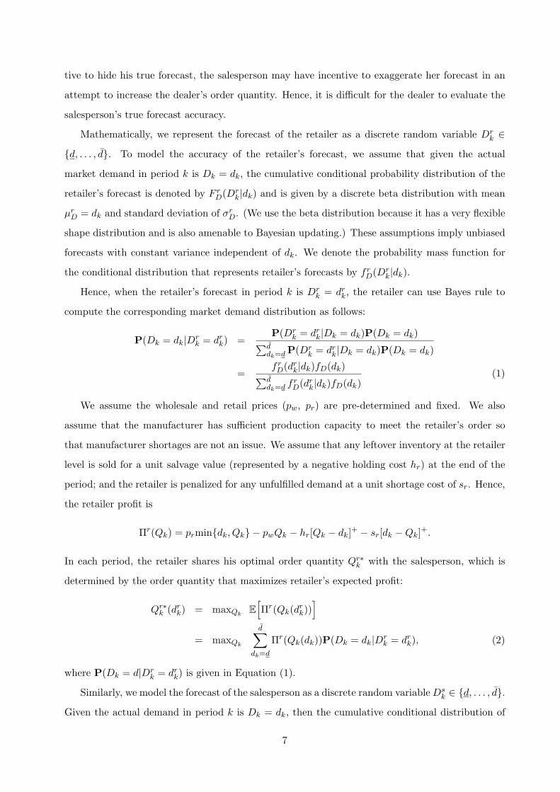
Mathematically, we represent the forecast of the retailer as a discrete random variable Drk ∈
{d, . . . , d}. To model the accuracy of the retailer’s forecast, we assume that given the actual
market demand in period k is Dk = dk, the cumulative conditional probability distribution of the
retailer’s forecast is denoted by F rD(Dr
k|dk) and is given by a discrete beta distribution with mean
µrD = dk and standard deviation of σr
D. (We use the beta distribution because it has a very flexible
shape distribution and is also amenable to Bayesian updating.) These assumptions imply unbiased
forecasts with constant variance independent of dk. We denote the probability mass function for
the conditional distribution that represents retailer’s forecasts by f rD(Dr
k|dk).
Hence, when the retailer’s forecast in period k is Drk = dr
k, the retailer can use Bayes rule to
compute the corresponding market demand distribution as follows:
P(Dk = dk|Drk = dr
k) =P(Dr
k = drk|Dk = dk)P(Dk = dk)∑d
dk=d P(Drk = dr
k|Dk = dk)P(Dk = dk)
=f r
D(drk|dk)fD(dk)∑d
dk=d f rD(dr
k|dk)fD(dk)(1)
We assume the wholesale and retail prices (pw, pr) are pre-determined and fixed. We also
assume that the manufacturer has sufficient production capacity to meet the retailer’s order so
that manufacturer shortages are not an issue. We assume that any leftover inventory at the retailer
level is sold for a unit salvage value (represented by a negative holding cost hr) at the end of the
period; and the retailer is penalized for any unfulfilled demand at a unit shortage cost of sr. Hence,
the retailer profit is
Πr(Qk) = prmin{dk, Qk} − pwQk − hr[Qk − dk]+ − sr[dk −Qk]+.
In each period, the retailer shares his optimal order quantity Qr∗k with the salesperson, which is
determined by the order quantity that maximizes retailer’s expected profit:
Qr∗k (dr
k) = maxQkE
[Πr(Qk(dr
k))]
= maxQk
d∑
dk=d
Πr(Qk(dk))P(Dk = dk|Drk = dr
k), (2)
where P(Dk = d|Drk = dr
k) is given in Equation (1).
Similarly, we model the forecast of the salesperson as a discrete random variable Dsk ∈ {d, . . . , d}.
Given the actual demand in period k is Dk = dk, then the cumulative conditional distribution of
7
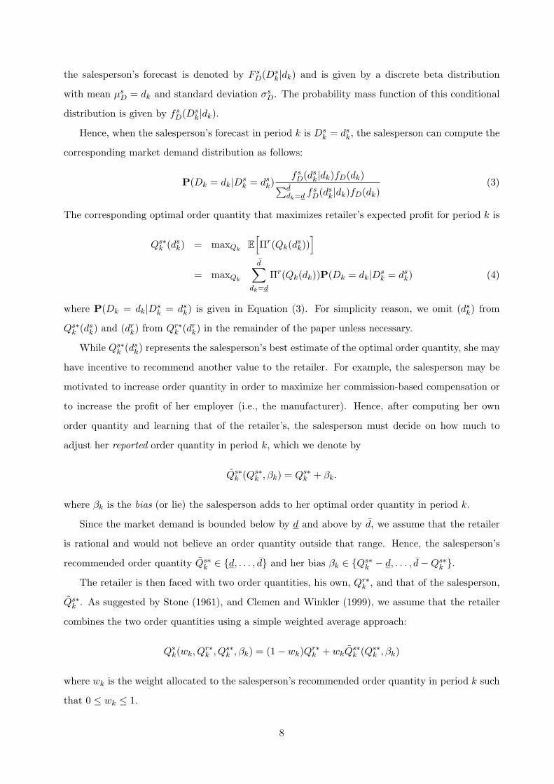
the salesperson’s forecast is denoted by F sD(Ds
k|dk) and is given by a discrete beta distribution
with mean µsD = dk and standard deviation σs
D. The probability mass function of this conditional
distribution is given by fsD(Ds
k|dk).
Hence, when the salesperson’s forecast in period k is Dsk = ds
k, the salesperson can compute the
corresponding market demand distribution as follows:
P(Dk = dk|Dsk = ds
k)f s
D(dsk|dk)fD(dk)∑d
dk=d f sD(ds
k|dk)fD(dk)(3)
The corresponding optimal order quantity that maximizes retailer’s expected profit for period k is
Qs∗k (ds
k) = maxQkE
[Πr(Qk(ds
k))]
= maxQk
d∑
dk=d
Πr(Qk(dk))P(Dk = dk|Dsk = ds
k) (4)
where P(Dk = dk|Dsk = ds
k) is given in Equation (3). For simplicity reason, we omit (dsk) from
Qs∗k (ds
k) and (drk) from Qr∗
k (drk) in the remainder of the paper unless necessary.
While Qs∗k (ds
k) represents the salesperson’s best estimate of the optimal order quantity, she may
have incentive to recommend another value to the retailer. For example, the salesperson may be
motivated to increase order quantity in order to maximize her commission-based compensation or
to increase the profit of her employer (i.e., the manufacturer). Hence, after computing her own
order quantity and learning that of the retailer’s, the salesperson must decide on how much to
adjust her reported order quantity in period k, which we denote by
Qs∗k (Qs∗
k , βk) = Qs∗k + βk.
where βk is the bias (or lie) the salesperson adds to her optimal order quantity in period k.
Since the market demand is bounded below by d and above by d, we assume that the retailer
is rational and would not believe an order quantity outside that range. Hence, the salesperson’s
recommended order quantity Qs∗k ∈ {d, . . . , d} and her bias βk ∈ {Qs∗
k − d, . . . , d−Qs∗k }.
The retailer is then faced with two order quantities, his own, Qr∗k , and that of the salesperson,
Qs∗k . As suggested by Stone (1961), and Clemen and Winkler (1999), we assume that the retailer
combines the two order quantities using a simple weighted average approach:
Q∗k(wk, Q
r∗k , Qs∗
k , βk) = (1− wk)Qr∗k + wkQ
s∗k (Qs∗
k , βk)
where wk is the weight allocated to the salesperson’s recommended order quantity in period k such
that 0 ≤ wk ≤ 1.
8

Research has shown that information provided by a trusted party is used more and considered
to have greater value to the trustor (Moorman et al. 1992, Glaeser et al. 2000). Hence, the
more the retailer trusts the salesperson, the more weight he puts on her recommendation. Because
placing a greater weight on the salesperson’s recommended order quantity has significant economic
consequences, it is an act of trust. Hence, we can view the weight on the salesperson’s forecast as
a measure of the retailer’s trust in the salesperson.
After the retailer purchases order quantity Q∗k, the actual market demand dk is realized. The
retailer compares the relative accuracy of his forecast to that of the salesperson and updates his
weight on salesperson’s recommendation in the next period wk+1.
Research has shown that individuals update trust in one another based on experience. Mayer et
al. (1995) proposed that in organizational relationships, “outcomes of trusting behaviors will lead
to updating of prior perceptions of the ability, benevolence and integrity of the trustee.” Kramer
(1999) suggested that decision makers assess interaction histories to provide a basis for drawing
inferences regarding their trustworthiness and for making predictions about the future behavior of
others. Hence, whenever the salesperson’s forecast is more accurate than the retailer’s, we would
expect the retailer’s perception of the salesperson’s ability and integrity to increase. However,
whenever the salesperson’s forecast is less accurate than that of the retailer, the retailer may
begin to doubt the honesty and/or competence of the salesperson. In our model, this implies that
the retailer adjusts his weight on the salesperson’s recommendation based on her past forecasting
accuracy.
We model the updating process using a simple model in which the weight in period k + 1, i.e.,
wk+1, is a linear combination of the weight in period k, i.e., wk, and the relative accuracy of the
salesperson’s forecast:
wk+1(wk, Qr∗k , Qs∗
k , βk, dk) = wk + δ(|dk −Qr∗
k | − |dk − Qs∗k (Qs∗
k , βk)|)
where δ is a sensitivity parameter that reflects the speed with which the retailer gains or loses trust
in the salesperson. Since the literature on trust suggests that the rates of gain or loss of trust may
not be symmetric (Wrightsman 1991; McKnight and Chervany 1996), we model δ via two separate
parameters, one for gains δg, and one for losses δl, such that:
δ ={
δg if |dk −Qr∗k | ≥ |dk − Qs∗
k |δl if |dk −Qr∗
k | < |dk − Qs∗k |
and δg, δl ≥ 0. When δg > δl, it is easier to gain the retailer’s trust than to lose it. We define a
retailer with this behavior as “trusting”. When δg < δl, it is harder to gain the retailer’s trust than
9

to lose it. We define a retailers with this behavior to be “skeptical”. For modeling purposes, we
will assume that both parties know δg and δl. In practice, the salesperson would have to estimate
the rates of trust gain and loss by analyzing the actual order quantities over time.
In addition to the rates of change over time, the initial trust level (i.e., initial weight w1), reflects
the ability of the salesperson to influence retailer decisions at the beginning of the relationship. This
initial weight can be affected by a variety of factors, including the salesperson’s reputation (Ganesan
1994, John and Weitz 1989), first impression from initial interactions (Ajzen and Fischibein 1980,
Mcknight et al. 1998), and the retailer’s emotional state and background (Gachter et al. 2004,
Jones and George 1998). Again, we will assume that the initial weight is known to both parties.
In practice, the salesperson can easily deduce this weight by observing the order quantity placed
by the retailer in the first period.
3.2 Model Formulation
To compute the salesperson’s optimal policy (i.e., what order quantities to recommend each period),
we make use of dynamic programming. Since we assume that excess inventory is sold at a reduced
price (a reasonable approximation of what happens at an auto dealership), inventory from previous
periods does not carry over. We consider a finite horizon with N periods, where N represents the
length of the relationship between the salesperson and the retailer. Later in this paper we study the
effects of the length of the relationship on salesperson’s behavior and on supply chain performance.
The state space when the number of remaining periods is j includes the current trust level (wj),
the salesperson’s optimal order quantity (Qs∗j ) and the retailer’s optimal order quantity (Qr∗
j ). We
can specify the dynamic program as follows:
• State Space S includes states (w,Qs∗, Qr∗), where Qs∗ = d, d+1, . . . d and Qr∗ = d, d+1, . . . d,and w ∈ [0, 1].
• Decision epochs are the beginning of every period after the retailer has offered his recom-mended order quantity.
• Action space A includes all values of possible bias that can be chosen by the salesperson.Since market demand is discrete and uniformly distributed on {d, d+1, . . . , d}, we know thatthe bias level β has to take values in increments of 1
n−1(d − d) (where n is the number ofdiscrete demand). Moreover, as discussed in Section 3.1, since the market demand is boundedabove and below, we know that β is also bounded such that β ∈ {Qs∗(ds)−d, . . . , d−Qs∗(ds)}.
We denote the value function where the number of remaining periods is j for state (wj , Qs∗j , Qr∗
j )
by Vj
[wj , Q
s∗j , Qr∗
j
], which represents the objective of the salesperson from period k = N − j until
the end of the time horizon (period k = N). Moreover, we define G(wj , Qs∗j , Qr∗
j , βj) to be the
10

component of the salesperson’s objective function that corresponds to the jth (remaining) period.
We write the optimality equation of the salesperson for period k = N − j as:
Vj
[wj , Q
s∗j , Qr∗
j
]= maxβj
{G(wj , Q
s∗j , Qr∗
j , βj)
+d∑
dj=d
d∑
Qs∗j−1=d
d∑
Qr∗j−1=d
Vj−1
[wj−1(wj , Q
r∗j , Qs∗
j , βj , dj), Qs∗j−1, Q
r∗j−1
]
P(dj |dsj)P(Qs∗
j−1, Qr∗j−1)
}(5)
where j = 1, 2, . . . , N . We know from equation (3) that
P(dj |dsj) =
P(dsj |dj)P(dj)
∑ddj=d P(ds
j |dj)P(dj).
Moreover, since Qs∗j−1 is a function of ds
j−1 and Qr∗j−1 is a function of dr
j−1 (equations 2 and 4) and
the salesperson knows the retailer’s forecast accuracy (i.e., P(drj−1|dj−1)), we find that
P(Qs∗j−1, Q
r∗j−1) =
d∑
dsj−1=d
d∑
drj−1=d
P(Qs∗j−1, Q
r∗j−1|ds
j−1, drj−1)P(ds
j−1, drj−1)
=d∑
dj−1=d
d∑
dsj−1=d
d∑
drj−1=d
P(Qs∗j−1, Q
r∗j−1|ds
j−1, drj−1)P(ds
j−1, drj−1|dj−1)P(dj−1)
On the other hand, since the retailer’s and salepserson’s forecasting processes are independent of
each other, we have
P(Qs∗j−1, Q
r∗j−1|ds
j−1, drj−1) = P(Qs∗
j−1|dsj−1)P(Qr∗
j−1|drj−1)
P(dsj−1, d
rj−1|dj−1) = P(ds
j−1|dj−1)P(drj−1|dj−1)
Thus, we will have
P(Qs∗j−1, Q
r∗j−1) =
d∑
dj−1=d
d∑
dsj−1=d
d∑
drj−1=d
P(Qs∗j−1|ds
j−1)P(Qr∗j−1|dr
j−1)P(dsj−1|dj−1)P(dr
j−1|dj−1)P(dj−1)
Note that probability P(Qs∗j−1|ds
j−1) (probability P(Qr∗j−1|dr
j−1)) is one, if in period j−1 the retailer’s
order size calculated by the salesperson (calculated by the retailer) based on her forecast dsj−1 (his
forecast drj−1) is Qs∗
j−1 (is Qr∗j−1); otherwise, this probability is zero.
We write the optimality equation of the salesperson in the last period (where j = 0) as:
V0
[w0, Q
s∗0 , Qr∗
0
]= maxβ0
{G(w0, Q
s∗0 , Qr∗
0 , β0)}
where 0 ≤ w0 ≤ 1, Qs∗0 = {d, d + 1, . . . d} and Qr∗
0 = {d, d + 1, . . . d}.
11

4 Benevolent Salesperson
In this section, we consider a salesperson that has the retailer’s best interests as her objective
function. This might be the case if the manufacturer uses a non-commission pay scheme that
motivates the salesperson to try to foster long term profitability of the retailer. We are interested
in: (i) will such a benevolent salesperson lie? (ii) if so, assuming the salesperson is rational, what
direction (i.e., overstating or understating) will she lie about the forecast? and (iii) how does this
behavior affect the supply chain performance?
We model the objective of the benevolent salesperson, which is to find the optimal bias in period
k (i.e., β∗k) such that the expected profit of the retailer is maximized, as follows:
β∗k = maxβk
N∑
l=k
E[Πr
l (Q∗l (βl))
]
We recall that Πr = prmin{dk, Q∗k}−pwQ∗
k−hr[Q∗k−dk]+−sr[dk−Q∗
k]+ where Qk = Q∗
k(wk, drk, d
sk, βk)
and N is the total number of periods. Hence, the salesperson chooses the optimal amount of bias
β∗ so as to maximize the sum of the retailer’s current profit and his expected profits from the future
periods. Therefore, function G(·) in (5) is Πr(wsj , Q
s∗j , Qr∗
j , βj), and (5) can be written as
Vj
[wj , Q
s∗j , Qr∗
j
]= maxβj
{Edj
[Πr(ws
j , Qs∗j , Qr∗
j , βj)]
+d∑
dj=d
d∑
dsj−1=d
d∑
drj−1=d
Vj−1
[wj−1(wj , Q
r∗j , Qs∗
j , βj , dj), Qs∗j−1, Q
r∗j−1
]
P(dj |dsj)P(Qs∗
j−1, Qr∗j−1)
}
and
V0
[w0, Q
s∗0 , Qr∗
0
]= maxβ0
{Πr∗(w0, Q
s∗0 , Qr∗
0 , β0)}
.
We determine the optimal policy for the benevolent salesperson using backward recursion.
4.1 Truthfulness and Trust of a Benevolent Salesperson
To gain insight into trust and its effect on the salesperson’s recommendations, we examined the
system behavior of 3240 cases using the above DP to compute the optimal policy and simulation
to generate demand outcomes for the following parameter ranges:
• Salesperson’s forecast accuracy 1σs : The salesperson’s forecast accuracy is characterized by the
standard deviation σs of her forecast distribution F sD. We considered values of the normalized
standard deviation to be 0.05, 0.1, and 0.2.
12

• Retailer’s forecast accuracy 1σr : The retailers’s forecast accuracy is characterized by the stan-
dard deviation σr of his forecast distribution F rD. We considered values of the normalized
standard deviation to be 0.05, 0.1, and 0.2.
• Retailer’s level of skepticism φ: Define φ = δl/δg. This ratio represents the relative ease
with which the salesperson loses the retailer’s trust as opposed to gaining it. A small ratio
represents a trusting retailer while a large ratio represents a skeptical retailer. We considered
values 0.5, 1, and 2.
• The critical order ratio z∗: Define z∗ = F−1(pr−pw+sr
pr+sr+hr) where F is the cumulative distribu-
tion of a standard normal distribution. This measure is the well-known critical ratio for a
newsvendor problem where demand is normally distributed. It characterizes the relative cost
of having too little inventory versus having too much. A negative ratio represents a case
where a high overage cost makes it optimal to order less than the average demand forecast.
A positive ratio represents a case where a high underage cost makes it optimal to order more
than the average demand forecast. We considered values −0.5, 0 and 0.5.
• Initial trust level w1: This measure represents the initial level of trust the retailer puts in the
salesperson’s recommended order quantity. We considered values 0, 0.25, 0.5, 0.75 and 1.
• Length of the relationship N : This is the total number of periods the salesperson will work
with the retailer. We considered values of 3, 6, 12, 24, 60, 120, 240, and 480. If periods
represent months, then this covers a range from three months to 40 years.
Note that the retailer revises his trust level wk after he observes the actual demand. Since
demand is stochastic, to attain a minimum confidence interval of 95% on the trust levels wk for
k = 1, 2, . . . , N , we conducted 2500 simulation replications for each case. In the remainder of
this section, we present our findings and discuss their implications for (i) the factors that promote
a benevolent salesperson to lie, (ii) the resulting level of trust, and (iii) the effect of lying on
trust, manufacturer’s profit and the retailer’s profit compared to those of a supply chain without a
salesperson.
We define B to be the overall bias, which is the average bias in the salesperson’s reported
forecast over the duration of the salesperson-retailer relationship, given by
B =1N
N∑
k=1
βk
Qs∗k
.
13

We also define W to be the overall trust, which is the average trust level over the duration of the
salesperson-retailer relationship, given by
W =1N
N∑
k=1
wk.
Among the 3240 simulation cases we considered, we found that the salesperson lies at least
once during the relationship in 96% of them. Moreover, 44% of the cases have a positive overall
bias, while 52% of the cases have a negative overall bias. We regard the benevolent salesperson’s
overstatement and understatement of order quantities as “white lies” because her intention is not
to harm the retailer but rather to help him.
Table 1. Average overall bias B for a benevolent salesperson.Critical Order Length of Relationship (N)
Ratio (z∗) 3 6 12 24 60 120 240 480 Average-0.50 1.3% 1.2% 1.1% 1.0% 1.1% 0.9% 0.8% 0.7% 1.0%0.00 -1.7% -1.3% -1.2% -1.0% -0.5% 0.2% -0.2% 0.0% -0.7%0.50 -2.2% -2.1% -1.5% -1.3% -0.9% -0.6% -0.4% -0.4% -1.2%
In Table 1, we summarize the average overall bias (B) of a benevolent salesperson for different
critical order ratios (z∗) and length of relationships (N). We find that bias moves inversely to
the critical order ratio. A benevolent salesperson is more likely to overstate her recommendation
when the cost of excess inventory is high (z∗ < 0) and a benevolent salesperson is more likely
to understate her recommendation when the cost of having a shortage is high (z∗ > 0). This is
because the retailer tends to shy away from ordering more stock when the cost of overage is high,
but he may over-order when the cost of shortage is high. The salesperson overstates or understates
her recommendation accordingly to overcome these tendencies. Note that this occurs regardless of
whether the salesperson is more or less accurate than the retailer. We also observe that a benevolent
salesperson is more likely to lie when the duration of the relationship is short. This is because, with
a limited time, she is willing to take the risk of losing the retailer’s trust in the future in order to
enhance the retailer’s short-term profit. Hence, we conclude the following:
Observation 1 It is not optimal for a salesperson to be entirely truthful even when she has the
retailer’s best interest at heart, but the extent of lying diminishes with the length of the retailer-
salesperson relationship.
In Table 2, we illustrate the overall trust level (W) of a benevolent salesperson for various
relative forecast accuracy (σs/σr) and relationship length (N).
We see that in cases where the salesperson has superior forecasting ability (σs/σr < 1), average
trust W increases as the relationship length N increases. In cases where the salesperson has inferior
14

forecasting ability (σs/σr > 1), average trust decreases as the relationship length increases. Hence,
the retailer’s trust in the salesperson is more reflective of the salesperson’s competence (i.e., forecast
accuracy) in a long term relationship than in a short-term relationship.
Table 2. Average overall trust W for a benevolent salespersonRelative Forecast Length of Relationship (N)Accuracy (σs/σr) 3 6 12 24 60 120 240 480 Average
0.25 0.53 0.57 0.69 0.81 0.92 0.96 0.98 0.99 0.810.5 0.51 0.54 0.60 0.68 0.81 0.87 0.91 0.92 0.731 0.42 0.44 0.45 0.46 0.46 0.45 0.45 0.44 0.452 0.41 0.42 0.39 0.34 0.22 0.16 0.14 0.13 0.284 0.41 0.40 0.36 0.30 0.20 0.14 0.08 0.06 0.24
Average 0.46 0.47 0.50 0.52 0.52 0.52 0.51 0.51 0.50
4.2 Value of a Benevolent Salesperson to Supply Chain Profits
In this section, we examine whether having a benevolent salesperson is beneficial for the manufac-
turer and the retailer in a supply chain. Specifically, we are interested in: (i) when the salesperson
has retailer’s best interest as her objective, does she always improve the retailer profit? and (ii)
does she ever increase manufacturer profit?
We use the superscripts “r” and “w” to represent the retailer and the manufacturer (wholesaler),
respectively. We denote the average profits over the duration of the salesperson-retailer relationship
by
Πr =1N
N∑
k=1
Πrk, Πw =
1N
N∑
k=1
Πwk
Note that, since we did not make any assumption about the salesperson’s compensation, the man-
ufacturer profit is the revenue it receives without taking into account of the salesperson’s compen-
sation cost. We also use the subscripts “ns” and “b” to represent the supply chains without a
salesperson and one with a benevolent salesperson, respectively.
Table 3.Average percentage increase in retailer’s profit if a benevolent salesperson is hired.Initial Trust Length of the Relationship (N)
(w1) 3 6 12 24 60 120 240 480 Average0.00 0.2% 0.6% 1.2% 2.0% 3.0% 3.5% 3.7% 3.8% 2.3%0.25 1.9% 2.0% 2.3% 2.8% 3.4% 3.7% 3.8% 3.9% 3.0%0.50 2.6% 2.7% 2.9% 3.2% 3.6% 3.8% 3.8% 3.9% 3.3%0.75 1.6% 1.8% 2.3% 2.8% 3.3% 3.6% 3.8% 3.9% 2.9%1.00 1.1% 1.2% 1.5% 2.1% 2.9% 3.4% 3.7% 3.9% 2.5%
Average 1.5% 1.6% 2.0% 2.6% 3.3% 3.6% 3.8% 3.9% 2.8%
To model a supply chain without a salesperson, we use the same modeling approach described in
Section 3.1 except with only one forecast from the retailer. For our tests, we considered parameter
ranges given in Section 4.1 and ran 2500 replications of each case.
15

As expected, retailer profit tends to be greater in (79% of the 3240 cases) in a supply chain
with a benevolent salesperson than without one. However, retailer profit in a supply chain with a
benevolent salesperson can be less (in 14% of the cases) than in one without a salesperson. Tables
3 and 4 show that this happens when (i) the salesperson’s forecasting skill is substantially worse
than the retailer’s (σs/σr = 2), (ii) the initial trust level is 100%, and (iii) the salesperson-retailer
relationship is very short (N ≤ 6). An initial trust level of 100% in a salesperson who is poor in
forecasting represents a case of misplaced trust. Moreover, when the time horizon is short, there is
limited opportunity for the retailer to appropriately lower his trust level in the salesperson based on
actual performance. While such an outcome is possible, we do not consider it very likely because an
incompetent salesperson would probably not project a sufficiently strong first impression to achieve
a 100% initial trust level. Hence, in most circumstances, a benevolent salesperson will improve
retailer profitability.
Table 4. Average percentage increase inretailer’s profit if a benevolent salesperson is hired.
Relative Forecast Retailer Skepticism (φ)Accuracy (σs/σr) 0.5 1 2 Average
0.25 15.3% 15.3% 16.0% 15.5%0.5 5.4% 6.0% 6.2% 5.9%1 0.2% 0.4% 0.0% 0.2%2 -1.2% -1.5% -1.6% -1.4%4 -1.5% -1.9% -2.0% -1.8%
Average 2.6% 2.6% 2.6% 2.6%
More interestingly, we find that while manufacturer profit tends to decrease (in 64% of the cases)
when he hires a benevolent salesperson, such a salesperson can sometimes increase manufacturer
profit (in 31% of the cases). Table 5 summarizes the percentage change in manufacturer profit from
a supply chain without a salesperson to one with a benevolent salesperson under different system
parameters.
Table 5. Average percent increase in manufacturer’s profit if a benevolent salesperson is hiredz∗ = −0.5 z∗ = 0 z∗ = 0.5
σr σr σr
σs 0.05 0.1 0.2 σs 0.05 0.1 0.2 σs 0.05 0.1 0.20.05 0.1% -6.3% -17.1% 0.05 0.2% -6.2% -18.8% 0.05 0.3% -6.6% -20.4%0.1 -0.2% -0.3% -9.9% 0.1 -0.2% -3.1% -4.2% 0.1 -2.4% 5.1% 3.9%0.2 -1.1% -4.1% -16.5% 0.2 -0.9% -1.8% 1.2% 0.2 -4.1% 8.5% 24.1%
Table 5 shows that a benevolent salesperson improves manufacturer profit most when (i) the
salesperson is less accurate than the retailer (i.e., σs ≥ σr), (ii) the retailer has a substantial amount
of forecasting error (σr ≥ 0.1), and (iii) the critical order ratio is high (z∗ = 0.5). When the
benevolent salesperson’s forecasting skill is poor and the cost of shortage is high, the salesperson is
likely to overstate her recommendation which encourages the retailer to order more than necessary.
16

Moreover, since the retailer’s forecast is poor, it is difficult for the retailer to appropriately adjust
his trust in the salesperson, which enables the salesperson to maintain her influence on the retailer.
Hence, the retailer’s poor forecast is coupled with the salesperson’s poor forecast, resulting in a
greater tendency for the retailer to over-order with a salesperson than without one. This promotes
manufacturer profit at the expense of the retailer.
5 Self-Serving Salesperson
Since it is very common for salespeople to be compensated in proportion to the volume of their
sales (e.g., in commission based compensation plans), we consider a self-serving salesperson whose
objective is to maximize the order quantity. Clearly, such an objective gives the salesperson in-
centive to inflate her recommended order quantity. But while inflating her recommendation may
boost the retailer order quantity, it will also undermine the retailer’s trust in future periods. Hence,
the salesperson needs to balance immediate and future gains when selecting an order quantity to
recommend to the retailer.
We model the objective of the self-serving salesperson as finding the optimal bias at each
period (i.e., β∗k) such that her expected total compensation is maximized. Since the salesperson’s
compensation is a linear function of the order size, the equivalent maximization problem is:
β∗k = maxβk
N∑
l=k
E[Q∗
l (βl)],
where N is the total number of periods in the salesperson-retailer relationship.
Hence, we can rewrite the dynamic programming model (5) for the self-serving salesperson as:
Vj
[ws
j , Qs∗j , Qr∗
j
]= maxβj
{Q∗
j (wj , Qs∗j , Qr∗
j , βj)
+d∑
dj=d
d∑
Qs∗j−1=d
d∑
Qr∗j−1=d
Vj−1
[wj−1(wj , Q
r∗j , Qs∗
j , βj , dj)Qs∗j−1, Q
r∗j−1
]
P(dj |dsj)P(Qs∗
j−1, Qr∗j−1)
}
and
V0
[w0, Q
s∗0 , Qr∗
0
]= maxβ0
{Q∗(w0, Q
s∗0 , Qr∗
0 , β0)}
Considering the same parameter ranges given in Section 4.1, we examine a supply chain with a
self-serving salesperson and discuss the implications of our results for (i) the factors that promote
a self-serving salesperson to lie, (ii) the process of trust building, and (iii) the effect of lying on
trust and profits compared to those of supply chains without a salesperson and with a benevolent
salesperson.
17
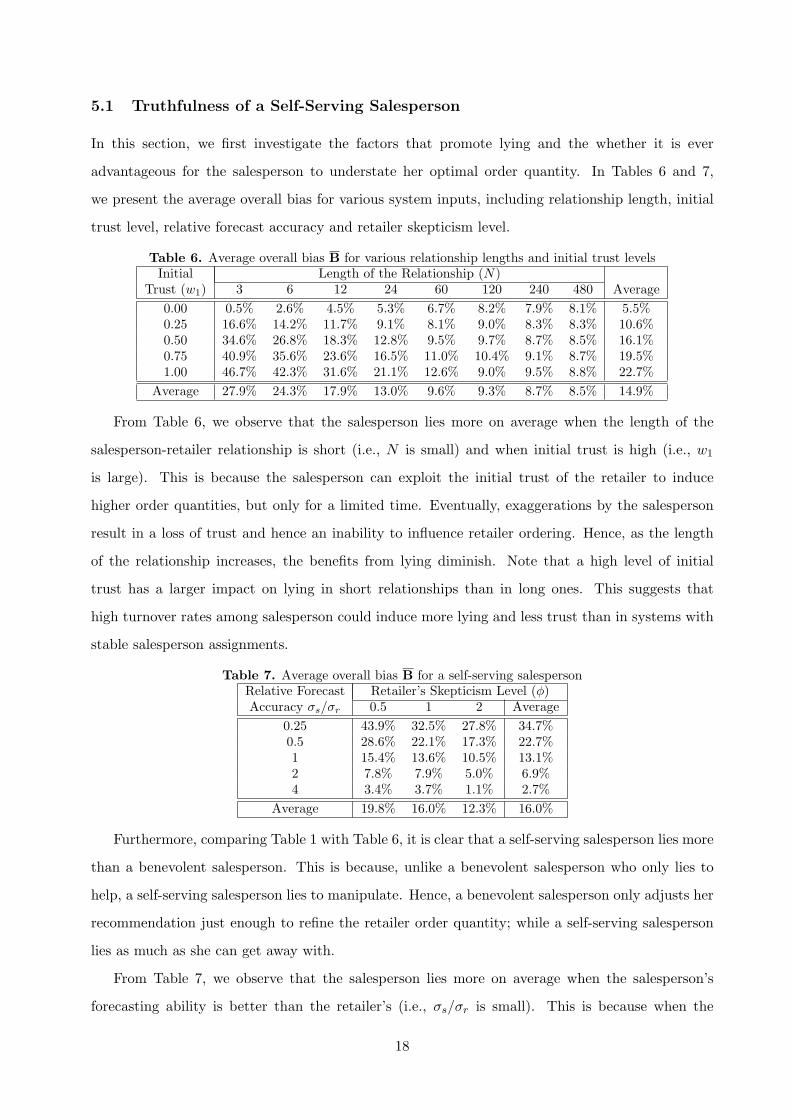
5.1 Truthfulness of a Self-Serving Salesperson
In this section, we first investigate the factors that promote lying and the whether it is ever
advantageous for the salesperson to understate her optimal order quantity. In Tables 6 and 7,
we present the average overall bias for various system inputs, including relationship length, initial
trust level, relative forecast accuracy and retailer skepticism level.
Table 6. Average overall bias B for various relationship lengths and initial trust levelsInitial Length of the Relationship (N)
Trust (w1) 3 6 12 24 60 120 240 480 Average0.00 0.5% 2.6% 4.5% 5.3% 6.7% 8.2% 7.9% 8.1% 5.5%0.25 16.6% 14.2% 11.7% 9.1% 8.1% 9.0% 8.3% 8.3% 10.6%0.50 34.6% 26.8% 18.3% 12.8% 9.5% 9.7% 8.7% 8.5% 16.1%0.75 40.9% 35.6% 23.6% 16.5% 11.0% 10.4% 9.1% 8.7% 19.5%1.00 46.7% 42.3% 31.6% 21.1% 12.6% 9.0% 9.5% 8.8% 22.7%
Average 27.9% 24.3% 17.9% 13.0% 9.6% 9.3% 8.7% 8.5% 14.9%
From Table 6, we observe that the salesperson lies more on average when the length of the
salesperson-retailer relationship is short (i.e., N is small) and when initial trust is high (i.e., w1
is large). This is because the salesperson can exploit the initial trust of the retailer to induce
higher order quantities, but only for a limited time. Eventually, exaggerations by the salesperson
result in a loss of trust and hence an inability to influence retailer ordering. Hence, as the length
of the relationship increases, the benefits from lying diminish. Note that a high level of initial
trust has a larger impact on lying in short relationships than in long ones. This suggests that
high turnover rates among salesperson could induce more lying and less trust than in systems with
stable salesperson assignments.
Table 7. Average overall bias B for a self-serving salespersonRelative Forecast Retailer’s Skepticism Level (φ)Accuracy σs/σr 0.5 1 2 Average
0.25 43.9% 32.5% 27.8% 34.7%0.5 28.6% 22.1% 17.3% 22.7%1 15.4% 13.6% 10.5% 13.1%2 7.8% 7.9% 5.0% 6.9%4 3.4% 3.7% 1.1% 2.7%
Average 19.8% 16.0% 12.3% 16.0%
Furthermore, comparing Table 1 with Table 6, it is clear that a self-serving salesperson lies more
than a benevolent salesperson. This is because, unlike a benevolent salesperson who only lies to
help, a self-serving salesperson lies to manipulate. Hence, a benevolent salesperson only adjusts her
recommendation just enough to refine the retailer order quantity; while a self-serving salesperson
lies as much as she can get away with.
From Table 7, we observe that the salesperson lies more on average when the salesperson’s
forecasting ability is better than the retailer’s (i.e., σs/σr is small). This is because when the
18
salesperson has better forecasting ability, she is more confident about her knowledge of the actual
demand and can better manipulate her recommended order quantity to maximize the retailer order
quantity. Armed with the power of knowledge, the self-serving salesperson can lie more without
causing the retailer to lose trust too quickly. The results in Table 7 also indicate that a salesperson
takes even more advantage of the power of accuracy when the retailer is a trusting in nature (i.e.,
φ is small).
Observation 2 On average, a self-serving salesperson lies more when (i) the salesperson has
better forecasting skills than the retailer, (ii) the overall length of the relationship is short,(iii)
initial trust is high, and (iv) retailer skepticism is low.
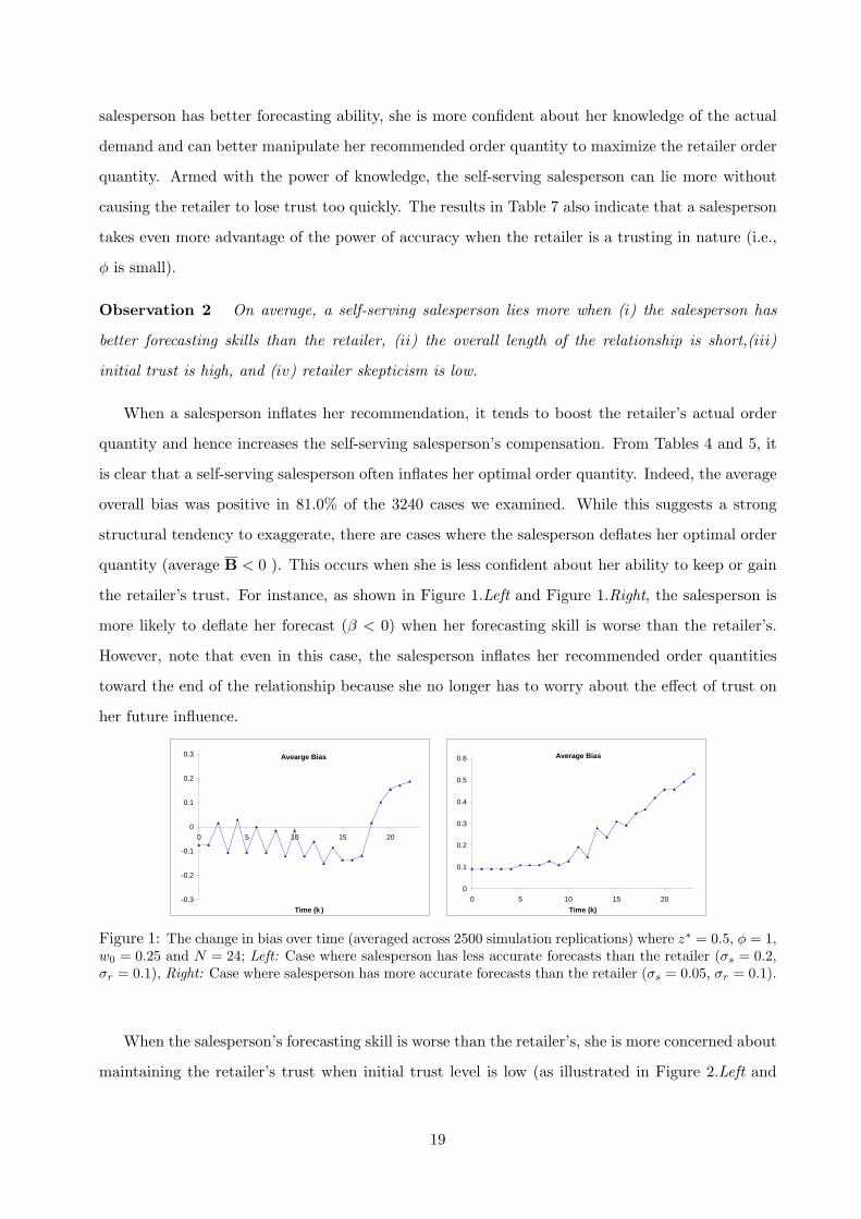
When a salesperson inflates her recommendation, it tends to boost the retailer’s actual order
quantity and hence increases the self-serving salesperson’s compensation. From Tables 4 and 5, it
is clear that a self-serving salesperson often inflates her optimal order quantity. Indeed, the average
overall bias was positive in 81.0% of the 3240 cases we examined. While this suggests a strong
structural tendency to exaggerate, there are cases where the salesperson deflates her optimal order
quantity (average B < 0 ). This occurs when she is less confident about her ability to keep or gain
the retailer’s trust. For instance, as shown in Figure 1.Left and Figure 1.Right, the salesperson is
more likely to deflate her forecast (β < 0) when her forecasting skill is worse than the retailer’s.
However, note that even in this case, the salesperson inflates her recommended order quantities
toward the end of the relationship because she no longer has to worry about the effect of trust on
her future influence.
-0.3
-0.2
-0.1
0
0.1
0.2
0.3
0 5 10 15 20
Time (k )
Avearge Bias
0
0.1
0.2
0.3
0.4
0.5
0.6
0 5 10 15 20
Time (k)
Average Bias
Figure 1: The change in bias over time (averaged across 2500 simulation replications) where z∗ = 0.5, φ = 1,w0 = 0.25 and N = 24; Left: Case where salesperson has less accurate forecasts than the retailer (σs = 0.2,σr = 0.1), Right: Case where salesperson has more accurate forecasts than the retailer (σs = 0.05, σr = 0.1).
When the salesperson’s forecasting skill is worse than the retailer’s, she is more concerned about
maintaining the retailer’s trust when initial trust level is low (as illustrated in Figure 2.Left and
19

-0.3
-0.2
-0.1
0
0.1
0.2
0.3
0 5 10 15 20
Time (k )
Avearge Bias
-0.1
0
0.1
0.2
0.3
0 5 10 15 20
Time (k )
Average Bias
Figure 2: The change in bias over time (averaged across 2500 simulation replications) where σs = 0.2,σr = 0.1, z∗ = 0.5, φ = 1, and N = 24; Left: Case where the initial trust is low (w1 = 0.25), Right: Casewhere the initial trust is high (w1 = 0.75).
-0.1
0
0.1
0.2
0.3
0 5 10 15 20
Time (k )
Average Bias
-0.3
-0.2
-0.1
0
0.1
0.2
0.3
0 20 40 60 80 100 120
Time (k )
Average Bias
Figure 3: The change in bias over time (averaged across 2500 simulation replications) where σs = 2, σr = 1,z∗ = 0.5, φ = 1, and w1 = 0.75; Left: Case where the salesperson-retailer relationship is short (N = 24),Right: Case where the salesperson-retailer relationship is long (N = 120).
Figure 2.Right), and when the relationship is fairly long (as illustrated in Figure 3.Left and Figure
3.Right). Hence, we conclude the following:
Observation 3 A self-serving salesperson tends to inflate her optimal order quantities to boost
retailer purchases. However, she sometimes deflates her order quantity recommendation when it is
difficult to retain trust, which occurs when (i) she is less accurate than the retailer, (ii) initial trust
is low, and (iii) the relationship is fairly long.
5.2 Evolution of Trust
In this section, we examine the evolution of trust and bias over the duration of the relationship.
Figure 4 illustrates a typical case for various initial trust levels. Figure 4.Left illustrates a scenario
where the relationship is fairly long and Figure 4.Right illustrates a scenario where the relationship
is fairly short.
We find that in most cases, regardless of initial trust level, trust converges fairly smoothly over
time to a steady level w (see Figure 4.Left). After an initial “warm up” period, trust holds steady at
20

0
0.2
0.4
0.6
0.8
1
0 50 100 150 200Time (k )
Average Trust
ws1=0ws1=0.25ws1=0.5ws1=0.75ws1=1.0
Average Trust
0
0.2
0.4
0.6
0.8
1
0 5 10 15 20Time (k )
ws1=0ws1=0.25ws1=0.5ws1=0.75ws1=1.0
0
0.2
0.4
0.6
0.8
1
0 50 100 150 200Time (k )
Average Bias
ws1=0ws1=0.25ws1=0.5ws1=0.75ws1=1.0
0
0.2
0.4
0.6
0.8
1
0 5 10 15 20Time (k )
Average Bias
ws1=0ws1=0.25ws1=0.5ws1=0.75ws1=1.0
Figure 4: The change of bias and trust over time (averaged across 2500 simulation replications) whereσs = 1, σr = 2, z∗ = 0.5, φ = 1; Left: Case where the salesperson-retailer relationship is long (N = 240),Right: Case where the salesperson-retailer relationship is short (N = 24).
w until near the end of the relationship when the salesperson takes advantage of the limited future
to ignore trust considerations. Note that the steady trust level w in the intermediate periods is
an indication of how much would retailer trust the salesperson if the relationship were to continue
forever. This steady state trust level depends heavily on the salesperson’s relative accuracy and
the retailer’s skepticism. The evolution of the salesperson’s bias follows a similar pattern. After a
“warm up” period, the amount of bias stabilizes and fluctuates around a steady level. Toward the
end of the relationship, bias increases significantly as the salesperson tries to boost order quantities.
Table 8. Average overall trust W for a self-serving salespersonRelative Forecast Length of Relationship (N)Accuracy (σs/σr) 3 6 12 24 60 120 240 480 Average
0.25 0.52 0.51 0.58 0.67 0.74 0.77 0.78 0.78 0.670.5 0.50 0.45 0.46 0.50 0.62 0.69 0.73 0.69 0.581 0.48 0.40 0.36 0.35 0.37 0.36 0.36 0.35 0.382 0.45 0.36 0.29 0.26 0.16 0.12 0.10 0.10 0.234 0.44 0.34 0.26 0.19 0.15 0.10 0.06 0.04 0.18
Average 0.48 0.41 0.39 0.39 0.41 0.41 0.41 0.39 0.41
When the salesperson-retailer relationship is fairly short, the trust level never stabilizes before
the “end of horizon” effect begins. Hence, initial trust in the early periods and manipulative
behavior by the salesperson in the late periods dominate the course of the relationship. Figure
4.Right illustrates an example of such behavior.
In Table 8, we further illustrate the effect of relationship length on the average trust of a
21
self-serving salesperson. Similar to the case for a benevolent salesperson, the retailer’s trust in a
self-serving salesperson is more reflective of the salesperson’s competence (i.e., forecast accuracy) in
a long term relationship than in a short-term relationship. However, from contrasting Table 8 with
Table 2, it is clear that a self-serving salesperson is less trusted than a benevolent salesperson. We
summarize our findings on how trust evolves and how it is affected by the length of the relationship
in the following observations:
Observation 4 Trust declines rapidly toward the end of a relationship because a self-serving
salesperson exaggerates her bias.
Observation 5 Increasing the length of the relationship improves the extent to which retailer trust
in the salesperson reflects the salesperson’s competence (i.e., forecast accuracy).
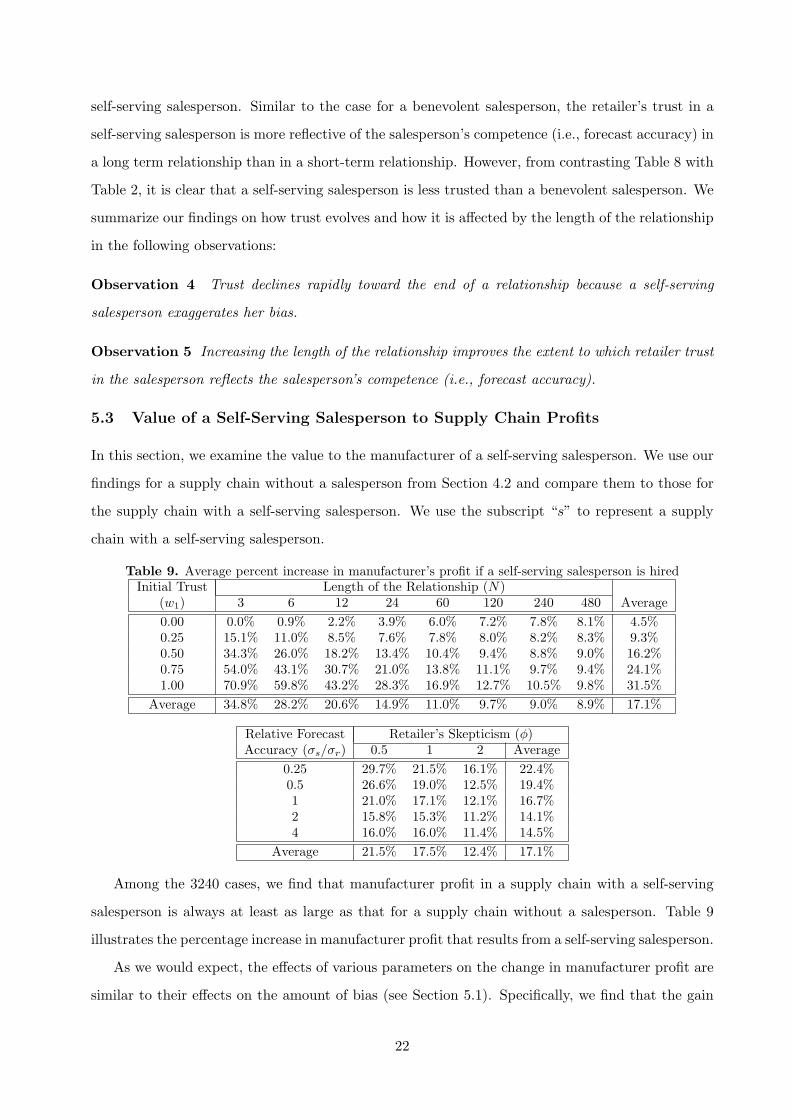
5.3 Value of a Self-Serving Salesperson to Supply Chain Profits
In this section, we examine the value to the manufacturer of a self-serving salesperson. We use our
findings for a supply chain without a salesperson from Section 4.2 and compare them to those for
the supply chain with a self-serving salesperson. We use the subscript “s” to represent a supply
chain with a self-serving salesperson.
Table 9. Average percent increase in manufacturer’s profit if a self-serving salesperson is hiredInitial Trust Length of the Relationship (N)
(w1) 3 6 12 24 60 120 240 480 Average0.00 0.0% 0.9% 2.2% 3.9% 6.0% 7.2% 7.8% 8.1% 4.5%0.25 15.1% 11.0% 8.5% 7.6% 7.8% 8.0% 8.2% 8.3% 9.3%0.50 34.3% 26.0% 18.2% 13.4% 10.4% 9.4% 8.8% 9.0% 16.2%0.75 54.0% 43.1% 30.7% 21.0% 13.8% 11.1% 9.7% 9.4% 24.1%1.00 70.9% 59.8% 43.2% 28.3% 16.9% 12.7% 10.5% 9.8% 31.5%
Average 34.8% 28.2% 20.6% 14.9% 11.0% 9.7% 9.0% 8.9% 17.1%
Relative Forecast Retailer’s Skepticism (φ)Accuracy (σs/σr) 0.5 1 2 Average
0.25 29.7% 21.5% 16.1% 22.4%0.5 26.6% 19.0% 12.5% 19.4%1 21.0% 17.1% 12.1% 16.7%2 15.8% 15.3% 11.2% 14.1%4 16.0% 16.0% 11.4% 14.5%
Average 21.5% 17.5% 12.4% 17.1%
Among the 3240 cases, we find that manufacturer profit in a supply chain with a self-serving
salesperson is always at least as large as that for a supply chain without a salesperson. Table 9
illustrates the percentage increase in manufacturer profit that results from a self-serving salesperson.
As we would expect, the effects of various parameters on the change in manufacturer profit are
similar to their effects on the amount of bias (see Section 5.1). Specifically, we find that the gain
22
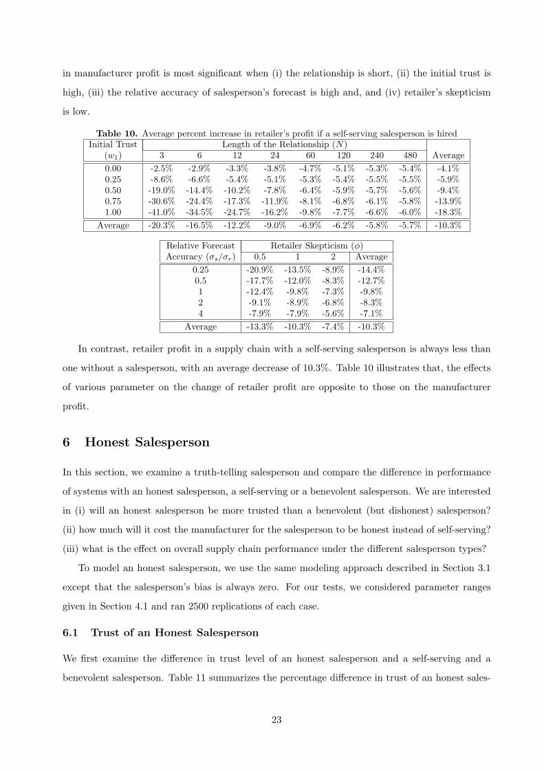
in manufacturer profit is most significant when (i) the relationship is short, (ii) the initial trust is
high, (iii) the relative accuracy of salesperson’s forecast is high and, and (iv) retailer’s skepticism
is low.
Table 10. Average percent increase in retailer’s profit if a self-serving salesperson is hiredInitial Trust Length of the Relationship (N)
(w1) 3 6 12 24 60 120 240 480 Average0.00 -2.5% -2.9% -3.3% -3.8% -4.7% -5.1% -5.3% -5.4% -4.1%0.25 -8.6% -6.6% -5.4% -5.1% -5.3% -5.4% -5.5% -5.5% -5.9%0.50 -19.0% -14.4% -10.2% -7.8% -6.4% -5.9% -5.7% -5.6% -9.4%0.75 -30.6% -24.4% -17.3% -11.9% -8.1% -6.8% -6.1% -5.8% -13.9%1.00 -41.0% -34.5% -24.7% -16.2% -9.8% -7.7% -6.6% -6.0% -18.3%
Average -20.3% -16.5% -12.2% -9.0% -6.9% -6.2% -5.8% -5.7% -10.3%
Relative Forecast Retailer Skepticism (φ)Accuracy (σs/σr) 0.5 1 2 Average
0.25 -20.9% -13.5% -8.9% -14.4%0.5 -17.7% -12.0% -8.3% -12.7%1 -12.4% -9.8% -7.3% -9.8%2 -9.1% -8.9% -6.8% -8.3%4 -7.9% -7.9% -5.6% -7.1%
Average -13.3% -10.3% -7.4% -10.3%
In contrast, retailer profit in a supply chain with a self-serving salesperson is always less than
one without a salesperson, with an average decrease of 10.3%. Table 10 illustrates that, the effects
of various parameter on the change of retailer profit are opposite to those on the manufacturer
profit.
6 Honest Salesperson
In this section, we examine a truth-telling salesperson and compare the difference in performance
of systems with an honest salesperson, a self-serving or a benevolent salesperson. We are interested
in (i) will an honest salesperson be more trusted than a benevolent (but dishonest) salesperson?
(ii) how much will it cost the manufacturer for the salesperson to be honest instead of self-serving?
(iii) what is the effect on overall supply chain performance under the different salesperson types?
To model an honest salesperson, we use the same modeling approach described in Section 3.1
except that the salesperson’s bias is always zero. For our tests, we considered parameter ranges
given in Section 4.1 and ran 2500 replications of each case.
6.1 Trust of an Honest Salesperson
We first examine the difference in trust level of an honest salesperson and a self-serving and a
benevolent salesperson. Table 11 summarizes the percentage difference in trust of an honest sales-
23
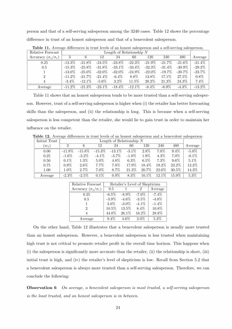
person and that of a self-serving salesperson among the 3240 cases. Table 12 shows the percentage
difference in trust of an honest salesperson and that of a benevolent salesperson.
Table 11. Average differences in trust levels of an honest salesperson and a self-serving salesperson.Relative Forecast Length of Relationship NAccuracy (σs/σr) 3 6 12 24 60 120 240 480 Average
0.25 -13.3% -21.8% -24.5% -23.8% -22.3% -21.9% -21.7% -21.6% -21.4%0.5 -15.3% -25.8% -31.8% -33.1% -33.4% -32.3% -31.4% -30.9% -29.2%1 -13.0% -25.0% -32.0% -32.0% -24.9% -22.0% -19.7% -20.7% -23.7%2 -11.2% -21.7% -21.4% -6.4% 8.8% 13.8% 17.1% 27.5% 0.8%4 -3.4% -12.1% -5.6% 3.2% 11.5% 20.2% 21.3% 24.3% 7.4%
Average -11.2% -21.3% -23.1% -18.4% -12.1% -8.4% -6.9% -4.3% -13.2%
Table 11 shows that an honest salesperson tends to be more trusted than a self-serving salesper-
son. However, trust of a self-serving salesperson is higher when (i) the retailer has better forecasting
skills than the salesperson, and (ii) the relationship is long. This is because when a self-serving
salesperson is less competent than the retailer, she would lie to gain trust in order to maintain her
influence on the retailer.
Table 12. Average differences in trust levels of an honest salesperson and a benevolent salesperson.Initial Trust Length of Relationship N
(w1) 3 6 12 24 60 120 240 480 Average0.00 -11.8% -15.8% -15.3% -13.1% -3.1% 2.8% 7.0% 9.4% -5.0%0.25 -1.6% -3.2% -4.1% -3.7% -1.0% 1.9% 4.3% 7.0% -0.1%0.50 0.1% 1.3% 5.0% 4.8% 6.3% 6.5% 7.3% 9.6% 5.1%0.75 0.9% 2.6% 7.7% 7.8% 17.9% 18.4% 19.2% 23.2% 12.2%1.00 1.0% 2.7% 7.0% 8.7% 21.3% 20.7% 22.6% 30.5% 14.3%
Average -2.3% -2.5% 0.1% 0.9% 8.3% 10.1% 12.1% 15.9% 5.3%
Relative Forecast Retailer’s Level of SkepticismAccuracy (σs/σr) 0.5 1 2 Average
0.25 -6.5% -8.9% -7.0% -7.4%0.5 -3.9% -4.6% -3.5% -4.0%1 3.0% -3.0% -4.1% -1.4%2 10.5% 13.5% 8.4% 10.8%4 44.0% 26.1% 16.2% 28.8%
Average 9.4% 4.6% 2.0% 5.3%
On the other hand, Table 12 illustrates that a benevolent salesperson is usually more trusted
than an honest salesperson. However, a benevolent salesperson is less trusted when maintaining
high trust is not critical to promote retailer profit in the overall time horizon. This happens when
(i) the salesperson is significantly more accurate than the retailer, (ii) the relationship is short, (iii)
initial trust is high, and (iv) the retailer’s level of skepticism is low. Recall from Section 5.2 that
a benevolent salesperson is always more trusted than a self-serving salesperson. Therefore, we can
conclude the following:
Observation 6 On average, a benevolent salesperson is most trusted, a self-serving salesperson
is the least trusted, and an honest salesperson is in between.
24

6.2 Differences in System Profits
In this section, we address the question of which type of salesperson, self-serving, benevolent or
honest, induces better supply chain performance. We first compare the system performance based
on manufacturer and retailer profits in Tables 13. Figure 5 illustrates the percentage difference
in retailer and manufacturer profits for a supply chain with an honest salesperson and one with a
self-serving/benevolent salesperson.
Table 13. Average Retailer’s and Manufacturer’s profitwith a benevolent salesperson, an honest salesperson and a self-serving salesperson
Length of Retailer’s Profit Manufacturer’s ProfitRelationship (N) Benevolent Honest Self-Serving Benevolent Honest Self-Serving
3 656.0 590.6 549.3 278.7 320.9 379.06 658.0 623.6 576.9 278.2 312.0 361.312 662.1 655.2 622.6 277.4 306.0 337.424 667.5 672.1 645.4 276.3 290.3 318.860 318.8 682.5 664.7 274.5 283.0 305.8120 682.8 680.7 665.2 273.2 277.2 295.2240 684.3 685.4 672.9 272.4 274.1 279.8480 698.5 695.4 685.3 272.0 272.2 275.4
Average 697.6 660.7 627.8 275.3 295.8 319.1
-15%
-10%
-5%
0%
5%
10%
15%
20%
0 100 200 300 400 500
Length of Relationship
Change in Retailer Profit
Benevolent Salesperson Self-Serving Salesperson
-20%
-15%
-10%
-5%
0%
5%
10%
15%
20%
0 100 200 300 400 500
Length of Relationship
Change in Manufacturer
Profit
Benevolent Salesperson Self-Serving Salesperson
Figure 5: Left: Percent increase in retailer’s profit (Πr) if an honest salesperson is replaced by a benevolentsalesperson or a self-serving salesperson; Right: Percent increase in manufacturer’s profit (Πw) if an honestsalesperson is replaced by a benevolent salesperson or a self-serving salesperson.
As we would expect, a benevolent salesperson always generates the greatest retailer profit and
the least manufacturer profit among the three kinds of salespersons. Moreover, a self-serving
salesperson always generates the greatest manufacturer profit and the least retailer profit. However,
the differences in system performance (for both the retailer and the manufacturer) diminish as
the relationship becomes longer. This is because when the relationship is long, the self-serving
salesperson cannot maintain trust unless her recommendation consistently outperforms that of the
retailer. Hence, it becomes more difficult for a self-serving salesperson to be manipulative in a long
term relationship. On the other hand, to make the best ordering decision in the long run, it is
beneficial for the retailer to know the actual accuracy of the salesperson and be able to account
25

for it accordingly. Hence, a benevolent salesperson tends to tell the truth and reveals her forecast
ability in a long-term relationship and behaves similar to an honest salesperson. We conclude the
following:
Observation 7 In long term relationships, the benefits to the manufacturer of a self-serving
salesperson, compared to a benevolent and an honest salespersons, are small.
Observation 8 In long term relationships, the benefits to the retailer of a benevolent salesperson,
compared to a self-serving and an honest salespersons, are small.
The insight here is that, given a sufficiently long time horizon, the need to gain retailer’s trust
forces a certain degree of truthfulness on the salesperson, which makes her almost benevolent. Since
trust is often necessary to promote other business functions beyond simple ordering transactions
(Covey 2006), it may actually be preferable for the manufacturer to incent salespersons to focus on
the interests of the retailer or simply, encourage the salespersons to be honest.
Lastly, we consider the total supply chain profit. Since the manufacturer can always share
profits with the retailer (e.g., via transfer payment, see Lee and Whang 1999 and Cachon 2003),
the salesperson that generates a higher total supply chain profit is likely to be the most beneficial
to both the manufacturer and the retailer. We define total supply chain profit Πt as the sum of the
manufacturer and retailer profits:
Πt = Πw + Πr.
We find that total supply chain profit with an honest salesperson is very close to that with a
benevolent salesperson. The average difference in total supply chain profit is is 0.9% while the
maximum and minimum differences are 4.2% and −3.7%, respectively.
Since total supply chain performance between an honest salesperson and a benevolent salesper-
son is very similar, we focus on comparing the performance between an honest salesperson and a
self-serving salesperson in the remainder of this section. We find that the total supply chain profit
is greater under an honest salesperson than under a self-serving salesperson in 73% of the cases;
and is lower under an honest salesperson than under a self-serving salesperson in the remaining
29% of the cases. Tables 14, 15, and 16 summarize the average percentage difference in total profit
for a supply chain with an honest salesperson and a supply chain with a self-serving salesperson.
Specifically, Table 14 illustrates cases where the retailer holding cost is negative (hr = −2.23),
which implies that the retailer can sell every unit of leftover inventory at the price of 2.23. Tables
15 and 16 illustrate the results for cases where leftover inventory at the retailer carries a low holding
26

cost (hr = 5) and a high holding cost (hr = 8.45), respectively.
Table 14. Percent increase in total supply chain profit when a benevolentsalesperson is replaced by a self-serving salesperson when salvage value is positive hr = −2.23Relative Forecast Length of Relationship (N)Accuracy (σs/σr) 3 6 12 24 60 120 240 480 Average
0.25 5.3% 5.4% 5.6% 5.5% 5.6% 5.5% 5.7% 5.7% 5.5%0.5 4.5% 4.2% 3.7% 3.6% 3.4% 3.5% 3.5% 3.3% 3.7%1 4.2% 3.5% 2.8% 2.4% 1.6% 1.5% 1.3% 1.3% 2.3%2 3.6% 2.7% 1.7% 0.9% 0.4% 0.2% 0.1% 0.1% 1.2%4 3.7% 2.8% 1.5% 0.9% 0.2% -0.1% -0.2% -0.3% 1.1%
Average 4.3% 3.7% 3.1% 2.7% 2.2% 2.1% 2.1% 2.0% 2.8%
Table 15. Percent increase in total supply chain profit when a benevolentsalesperson is replaced by a self-serving salesperson when retail holding cost is low hr = 1.00
Relative Forecast Length of Relationship (N)Accuracy (σs/σr) 3 6 12 24 60 120 240 480 Average
0.25 -3.1% -2.9% -2.8% -2.8% -2.9% -2.9% -2.9% -2.7% -2.9%0.5 -2.1% -1.9% -1.7% -1.6% -1.6% -1.5% -1.5% -1.5% -1.7%1 -1.4% -1.1% -0.7% -0.5% -0.4% -0.4% -0.4% -0.4% -0.7%2 -0.3% -0.3% -0.1% -0.3% -0.2% -0.4% -0.5% -0.5% -0.3%4 0.6% 0.5% 0.4% 0.3% 0.1% 0.1% 0.1% 0.1% 0.3%
Average -1.3% -1.1% -1.0% -1.0% -1.0% -1.0% -1.0% -1.0% -1.1%
Table 16. Percent increase in total supply chain profit when a benevolentsalesperson is replaced by a self-serving salesperson when retail holding cost is high hr = 8.45
Relative Forecast Length of Relationship (N)Accuracy (σs/σr) 3 6 12 24 60 120 240 480 Average
0.25 -20.1% -18.9% -17.9% -18.1% -18.2% -18.3% -18.3% -18.3% -18.5%0.5 -18.6% -16.7% -14.7% -13.6% -13.2% -13.1% -13.0% -13.0% -14.5%1 -16.6% -14.0% -10.9% -8.6% -6.9% -6.4% -6.2% -5.8% -9.4%2 -14.7% -11.4% -7.7% -4.8% -3.2% -2.8% -2.6% -2.5% -6.2%4 -12.2% -8.8% -5.2% -2.7% -1.2% -0.7% -0.4% -0.3% -3.9%
Average -16.4% -14.0% -11.3% -9.5% -8.5% -8.2% -8.1% -8.0% -10.5%
Comparing Tables 14, 15, 16, it is clear that a self-serving salesperson is more beneficial to total
supply chain profit when the retailer holding cost is low. The reason for this is as follows. Given
the wholesale price in this model is fixed at pw = 5, a low holding cost results in a high wholesale
price to holding cost ratio. Similarly, a high holding cost results in a low wholesale price to holding
cost ratio. In cases where the ratio of wholesale price and holding cost is high, as the order quantity
increases, the rate of increase in manufacturer profit is greater than the rate of decrease in retailer
profit. Since a self-serving salesperson tends to promote a greater order quantity than a benevolent
salesperson, when the wholesale price to holding cost ratio is high, the increase in manufacturer
profit is likely to compensate for the decrease in retailer profit, which improves total supply chain
profit.
Finally, it is clear from Table 13 that the increase in total supply chain profit from replacing an
honest salesperson cases with a self-serving salesperson is large when : (i) the relationship is short,
and (ii) the salesperson’s forecasting skill is superior to the retailer’s. This is because a shorter
27
relationship and superior forecasting skill gives the self-serving salesperson more power to inflate
her recommendation. Hence, the total supply chain profit is increased to a greater extent when the
wholesale price to retailer holding cost ratio is high. We conclude the following:
Observation 9 A benevolent salesperson and an honest salesperson generate similar level of total
supply chain profits.
Observation 10 On average, an honest salesperson tends to generate greater total supply chain
profit than a self-serving salesperson. However, a self-serving salesperson can generate greater total
supply chain profit when (i) the ratio of wholesale price to retailer holding cost is high, (ii) the
overall length of the relationship is short, and (iii) the salesperson has better forecasting skills than
the retailer.
7 Summary
While it is widely acknowledged in industry that relational factors play an important role in supply
chain performance and coordination, operations management research has generally relegated such
issues to the category of “intangibles”. At best, the development of trust has been modeled a
something that evolves in a “black box” and is therefore not directly addressed. In this study, we
have made a preliminary step toward modeling trust as a dynamic and quantifiable component in
supply chain decisions. This has allowed us to examine the evolution of trust and its impact on the
supply chain members’ behavior.
We find that a benevolent salesperson who focuses on retailer profit does not necessarily tell the
truth. In fact, she occasionally tells white lies to increase retailer profit. In contrast, a self-serving
salesperson manipulates the retailer to order more stock by lying, particularly when her forecasting
skill is superior to that of the retailer and when the initial trust on the part of the retailer is high.
A self-serving salesperson also exploits the trust she builds in the early part of a relationship to lie
excessively toward the end of the relationship.
In terms of supply chain performance, a benevolent salesperson always generates less manufac-
turer profit, but more retailer profit, than a manipulative self-serving salesperson and a truth-telling
salesperson. Furthermore, while a benevolent salesperson and an honest salesperson generate very
similar total supply chain profit, an honest salesperson is more likely to generate greater total
supply chain profit than a self-serving salesperson. However, if the wholesale price is significantly
greater than the retail holding cost, a self-serving salesperson can improve the total supply chain
profit. Under these circumstances, a manufacturer can always share profit with the retailer, so it
28

is possible for a self-serving salesperson to benefit the retailer.
In general, regardless of how manipulative a self-serving salesperson is, time (i.e., duration
of the relationship) has the power to reveal her competence (i.e., actual forecast ability). In a
long term relationship, a self-serving salesperson is more cautious about the tradeoff of immediate
gain (current order quantity) and value of future cooperation (which affects future orders). As a
result, differences in order quantity, manufacturer profit and retailer profit under a self-serving
salesperson and a benevolent salesperson become fairly small as the time horizon grows long.
Benevolent actions induce greater trust in the salesperson-retailer relationship, which may yield
benefits in other aspects of the business relationship and offset the small decrease in commissions.
This suggests that in long term supply chain relationships where trust is vital, job assignments
and salesforce incentives that promote a focus on long term relationships can benefit both the
manufacturer and retailer in a supply chain.
In this paper, we have focused on trust only in the context of forecast sharing. To develop a
more comprehensive understanding of the impact of trust on other aspects of supply chain coordi-
nation, further modeling work is needed. For instance, it would be useful to consider a salesperson
who performs multiple tasks, possibility including demand promotion and inventory allocation, in
addition to forecast sharing, and examine the impact of trust building on the salesperson’s effec-
tiveness in the other tasks. It would also be interesting to extend the analysis of trust to a supply
chain with various types of supply chain contracts. The goal would be to discover how trust affects
the optimal contract structure, and how to strike an appropriate balance between formal contracts
and informal trust as promoted by salesperson incentives.
References
Ajzen, I., and M. Fischbein. 1980. Understanding Attitudes and Predicting Social Behavior.Prentice-Hall: Englewood Cliffs, NJ.
Anderson, E., and A. T. Coughlan. 2002 Channel management: structure, governance, andrelationship management, in B. Weitz and R. Wensley (eds), Handbook of Marketing SagePublications: Thousand Oaks, California.
Aviv Y. 2001. The effect of collaborative forecasting on supply chain performance. ManagementScience 47(10):1326-1344.
Aviv Y. 2004. Collaborative forecasting and its impact on supply chain performance, in Simchi-Levi D., S. D. Wu, and Z. Shen (eds), Handbook of Quantitative Supply Chain Analysis:Modeling in the E-Business Era Kluwer:Norwell, MA.
Berg, J., J. Dickhaut, K. McCabe. 1995. Trust, reciprocity, and social history. Games andEconomic Behavior 10:122-142.
29

Ben-Zion, U., Cohen, Y, Peled, R. and Shavit, T. (2005). Decision-making and the newsvendorproblem: An experimental study. Ben-Gurion University. Working paper, BeerSheva, Isreal.
Bernheim, B. D., and M. D. Whinston 1998. Incomplete contracts and strategic ambiguity. Amer-ican Economic Review 88:902932.
Bohnet, I., and R. Zeckhauser. 2004. Trust, risk and betrayal. Journal of Economic Behaviorand Organization Vol. 55:467484.
Bolton, G. and Katok, E. (2005), Learning-by-doing in the newsvendor problem: A laboratoryinvestigation. Penn State University. Working Paper, University Park, PA.
Cachon, G. P., and M. Fisher. 2000. Supply chain inventory management and the value of sharedinformation. Management Science 46(8):1032-1048.
Cachon, G. P., and M. A. Lariviere. 2001. Contracting to assure supply: how to share demandforecasts in supply chain. Management Science 47(5):629-647.
Cachon, G. P. 2003. Supply chain coordination with contracts, in A. G. de Kok and S. C.Graces (eds), Handbooks in Operations Research and Management Science , Vol 11. Elsevier:Amsterdam, Netherlands.
Carnevale, P., and A. M. Isen. 1986. The influence of positive affect and visual access on the dis-covery of integrative solutions in bilateral negotiation. Organizational Behavior and HumanDecision Processes 37:1-13
Chen, F. 2003. Information sharing and supply chain coordination, in de Kok A. G. and S.C .Graves (eds), Handbooks in Operations Research and Management Science Volume 11.Elsevier: Amsterdam.
Clemen, R. T., and R. L. Winkler. 1999. Combining probability distributions from experts in riskanalysis. Risk Analysis 19(2):187-203.
Crosby, L. A., K. R. Evans, D. Cowles. 1990. Relationship quality in services selling - an inter-personal influence perspective. Journal of Marketing 54(3):68-81.
Covey, S. M. R. 2006 The speed of trust. CoveyLink: New York, NY.
Doney, P. M., and J. P. Cannon. 1997. An examination of the nature of trust in buyer-sellerrelationships. Journal of Marketing 61(April):307-319.
Engle-Warnick, J., and R. L. Slonim. 2004. The evolution of strategies in a repeated trust game.Journal of Economic Behavior and Organization 55:553-573.
Ganesan, S. 1994. Determinants of long-term orientation in buyer-seller relationships. Journal ofMarketing 58(2):1-19.
Gachter, S., B. Herrmann, and C. Thonia. 2004. Trust, voluntary cooperation, and socio-economicbackground: survey and experimental evidence. Journal of Economic and Organization55:505-531.
30

Glaeser, E. L., D. I. Laibson, J. A. Scheinkman, and C. L. Soutter. 2000. Measuring trust.Quarterly Journal of Economics 115(3):811-847.
Handfielda, R. B., and C. Bechtel. 2002. The role of trust and relationship structure in improvingsupply chain responsiveness. Industrial Marketing Management 31:367382.
Hopp, W. J., S. M. R. Iravani, and G. Yuen. 2006. The role of salespersons and incentives insupply chain performance. Working paper, Northwestern University, Evanston, IL.
John, G. and B. Weitz. 1989. Salesforce Compensation: An Empirical Investigation of FactorsRelated to Use of Salary versus Incentive Compensation. Journal of Marketing Research26(1): 1-14.
Jones, G. R. and J. M. George. 1998. The experience and evolution of trust: implications forcooperation and teamwork. Academy of Management Review 23(3):531-546.
Jones, T.M. 1995. Instrumental stake holder theory: a synthesis of ethics and economics. Academyof Management Review 20: 404-437.
Keser, C. and Paleologo, G. (2004), Experimental investigation of retailer-supplier con- tracts:The wholesale price contract. IBM Research Working Paper. Yorktown, NY.
Kollock, P. 1994. The emergence of exchange structures: an experimental study of uncertaintycommitment and trust. American Journal of Sociology 100:313-345.
Kramer, R. M. 1999. Trust and Distrust in Organizations: Emerging Perspectives, EnduringQuestions. Annual Review of Psychology 50:569-598.
Larzelere, R. E., and T. L. Huston. 1980. The dyadic trust scale: toward understanding interper-sonal trust in close relationships. Journal of Marriage and the Family 42(3):595-604.
Lee H, and S. Whang. 1999. Decentralized Multi-Echelon Supply Chains: Incentives and Infor-mation. Management Science 45(5): 633-640.
Lewicki, R. J., and B. B. Bunker. 1995. Trust in relationships: a model of development and decline,in B. B. Bunker, J. Z. Rubin, and Associates (eds.) Conflict, Cooperation and Justice: Essaysinspired by the work of Morton Deutsch 133-174. Jossey-Bass: San Francisco, CA.
Malhotra, D., and J. K. Murnighan. 2002. The effects of contract on interpersonal trust. Admin-istrative Science Quarterly 47:534-559.
Mayer, R. C., J. H. Davis, and F.D. Schoorman. 1995. An integrative model of organizationaltrust. Academy of Management Review 20(3):708-734.
McKnight, D. H., and N. L. Chervany. 1996. The meanings of trust. University of Minnesota.Working paper, Minneapolis, MN.
McKnight D. H., L. L. Cummings, and N. L. Chervany. 1988. Initial Trust Formation in NewOrganizational Relationships. The Academy of Management Review 23(3): 473-490.
31

Mellinger, G. D. 1956. Interpersonal trust as a factor in communication. Journal of AbnormalPsychology 52(3):304-309.
Moorman, C., R. Deshpande, and G. Zaltman. 1992. Relationships between providers and usersof market research: the dynamics of trust within and between organizations, Journal ofMarketing Research. 29(August): 314-28.
Narayanan, V. G., and A. Raman. 2004. Aligning incentives in supply chain. Harvard BusinessReview. November(R0411F).
Ren, Z. J., M. A. Cohen, T. H. Ho, C. Terwiesch. 2004. Sharing forecast information in along-term supply chain relationship. Boston University. Working paper, Boston, MA.
Rousseau D. M., S. B. Sitkin, R. S. Burt, and C. Camerer. 1998. Not so different after all: Across-discipline view of trust . Academy of Management Review 3(3):393-404.
Schweitzer, M. and Cachon, G. (2000), Decision bias in the newsvendor problem: experimentalevidence. Management Science 46(3), 404-420.
Smith, K. G., S. J. Carroll, and S. J. Ashford. 1995. Intra- and Interorganizational Cooperation:Toward a Research Agenda. Academy of Management Journal 38:7-23.
Stone, M. 1961. The opinion pool. Annals of Mathematical Statistics 32:13391342.
Tardy, C. H. 1988. Interpersonal evaluations: measuring attraction and trust. A handbook for thestudy of human communications. Ablex Publishing: Norwood, NJ.
Taylor, T. A., and E. L. Plambeck. 2003. Supply chain relationships and contracts: The impact ofrepeated interaction on capacity investment and procurement. Stanford University. Workingpaper, Palo Alto, CA.
Terwiesch, C., Z. Justin Ren, Teck H. Ho, and Morris A. Cohen. 2005. An Empirical Analysisof Forecast Sharing in the Semiconductor Equipment Supply Chain. Management Science51(2): 208-220.
Thompson, L. L. 1991. Information Exchange in Negotiation. Journal of Experimental Psychology27:61-179.
Tsay, A., N. Agrawal. 1999. Channel conflict and coordination: an investigation of supply chaindesign. Santa Clara University. Working Paper, Santa Clara, CA.
Uzzi, B. 1996. The sources and consequences of embeddedness for the economic performance oforganizations: the network effect. American Sociological Review 61:674-698.
Wrightsman, L. S. 1991. Interpersonal trust and attitudes toward human nature. in Robinson, J.P., Shaver, P. R., and Wrightsman, L. S. (eds.), Measures of personality and social psycho-logical attitudes, Vol 1. San Diego, CA: Academic Press.
Zaheer, N., and A. Venkatraman. 1995. Relational governance as an interorganizational strategy:an empirical test of the role of trust in economic exchange. Strategic Management Journal16(55):372-392.
32