true coincidence summing corrections -...

172

Chapter -6

True Coincidence Summing

Corrections

6.1 Introduction

6.2 True Coincidence Summing

6.2.1 General Overview

6.2.2 Factors affecting true coincidence summing

6.2.3 Methods for coincidence correction

6.3 Objective of the work

6.4 Gamma spectrometric measurements

6.4.1 Standardization of gamma sources

6.4.2 Efficiencies of point sources at different distances

6.5 Coincidence summing correction for point source geometry

6.5.1 Coincidence summing correction factors by analytical method

6.5.2 Validation of the analytical method

6.5.3 Application of the method

6.6 Coincidence summing correction for volumetric sources

6.7 Conclusion

Chapter 6

173

6.1 Introduction

As discussed in Chapter 1 of this thesis, true coincidence summing (TCS) is one of the

factors which may lead to non-proportionality between the measured count rate and the

mass of the nuclide monitored. True coincidence summing takes place when two or more

gamma rays (or a gamma ray and an X-ray) which are emitted in a cascade from an

excited nucleus are detected within the resolving time of the detector. As a result, the

detector cannot distinguish between the two interactions, and treats them as a single

event, the energy transfer being the sum of the two interactions. This leads to a loss in

count from the peaks corresponding to two gamma rays and addition of count at the sum

of two energies. This results in inaccurate count rate and hence erroneous results. The

coincidence correction factor (kTCS) is defined as the ratio of the count rate in absence of

the coincidence to the count rate in presence of coincidence:

(6.1)

6.2 True Coincidence Summing

6.2.1 General Overview

If two gamma rays with energies E1 and E2 are in coincidence with each other, then there

may be summing in and summing out effects resulting from the addition of counts at the

energy corresponding to the sum of two energies (E1+E2) and loss of counts from the two

peaks (E1, E2) respectively. For example, 60Co decays by β- to 60Ni and emits 1173 and

1332 keV gamma rays in cascade (Figure 6.1). These two gamma rays may reach the

detector at the same time and can sum up to give counts at 2505 keV in the spectrum. The

( )( )TCS

Count rate or in absenceof coincidencekCount rate or in presenceof coincidence

εε

=

Chapter 6

174

loss in count rate at 1173 keV and 1332 keV is known as summing out event. In this case

since a peak at 2505 keV already exists although the probability is very low, so there will

be an increase in counts at that peak and this is known as summing in event. When there

is no gamma ray corresponding to E1+E2 then new peak may appear at this energy. In the

former case, the correction factor (as given by equation 6.1) will be less than unity and in

the latter case it will be greater than unity.

6027Co (5.2714 y)

6028Ni

99.925 %

0.067 %

0+

2+

4+

5+ Summing Out

Summing In

Figure 6.1 True coincidence summing effects in the beta decay of 60Co.

Each sum peak represents only a small part of the total counts lost from the full energy

peaks. This is because there will be a chance of summing of a particular gamma ray with

each and every gamma ray in the cascade whether or not fully absorbed. In fact, since

only a minority of gamma rays is fully absorbed, the summing of a gamma ray destined

for a full energy peak with an incompletely absorbed gamma ray is more likely.

Chapter 6

175

Therefore, the coincidences with partially absorbed gamma rays must be taken into

account if a TCS correction is to be done.

6.2.2 Factors Affecting True Coincidence Summing The extent of coincidence summing depends upon the probability that two gamma rays

emitted simultaneously will be detected simultaneously [Gilmore (2008)]. Therefore,

these effects are independent of count rate of the source and depend solely on the

emission probabilities and detection efficiencies of the cascade gamma rays. The

emission probabilities of different gamma rays are characteristic of the radionuclide

under study. The detection efficiencies are function of the solid angle subtended by the

source at the detector i.e., the source-to-detector distance and the area of the detector

front face. As shown in Figure 6.2, if there are two sources S1 and S2 of equal strengths

with S1 placed on the detector end cap and S2 placed at some distance, since the solid

angle subtended by S1 will be greater than S2, the probability of the two gamma rays

reaching the detector simultaneously will be more in the former case leading to

significant coincidence corrections at closer distance.

6.2.3 Methods for Coincidence Correction

The coincidence summing corrections can be avoided by counting the sample far from

the detector, so that the probability of two gamma rays reaching the detector at the same

time is negligible. This is quite impractical for samples with low activity eg.

environmental samples where the samples are required to be counted as close as possible

to the detector. Another way to avoid coincidence summing corrections is to use a

gamma ray standard of the same radionuclide as the one monitored. This may be practical

Chapter 6

176

for a routine lab where few radionuclides are monitored and one can have a set of

standards corresponding to those nuclides. But if a variety of samples are to be analyzed

such as environmental, fission product, activation product samples etc. then to have

gamma ray standards of all the radionuclides is next to impossible and it is better to apply

true coincidence summing correction. As an example, the importance of TCS corrections

has been discussed in ref. [Garcia-Talavera et al. (2001)] for the measurement of

radionuclides in natural decay series using gamma ray spectrometry.

DetectorEnd cap

S1

S2

Figure 6.2 Effect of solid angle on true coincidence summing effects.

Analytical approach

A general method for computing coincidence correction factors was first demonstrated by

Andreev et al. (1972) and has been further developed and applied in practice by other

authors [Andreev et al. (1973), Debertin and Schotzig (1979), Mccallum and Coote

(1975), Sinkko and Aaltonen (1975), Schima and Hoppes (1983), Dryak and Kovar

Chapter 6

177

(2009), Corte and Freitas (1992), Montgomery and Montgomery (1995), Kafala (1995),

Sundgren (1993), Richardson and Sallee (1990)]. This is an analytical approach which

requires the use of full energy peak and total efficiencies and information about the

nuclear decay parameters such as the mode of parent nuclide decay, energies of gamma

transitions, gamma ray emission probabilities, K-capture probabilities (in electron capture

decay), mean energy of K X-rays, fluorescence yield, total and K conversion coefficients

etc. All these factors are used to calculate the probability of simultaneous emission of two

or more cascade gamma rays.

In this method, the true coincidence correction (kTCS) is, in general given by:

1

1

1TCS i n

i t ii

kp ε

=

=

=− ∑

(6.2)

where, n is total number of gamma rays in coincidence with gamma ray of interest, pi

represents the probability of simultaneous emission of ith gamma and the gamma ray of

interest and εti represents the total efficiency of ith gamma ray. In order to calculate kTCS

by this method, the probability pi is calculated by taking into account appropriate

parameters obtained from the published decay schemes of the radionuclides [Dias et al.

(2002)]. This method can be understood in a better way by the following example:

Consider a nuclide X decaying to Y by beta decay as shown in Figure 6.3.

The nuclide X decays to the two excited states of Y. The two excited states deexcite by

emission of three gamma rays γ1 (2 → 1), γ2 (1 → 0) and γ3 (2 → 0) with their respective

probabilities as p1, p2 and p3. In absence of coincidence summing, the count rate is

given by:

Chapter 6

178

10 1 1N Ap ε= (6.3)

where A is the disintegration rate of the source and ε1 is the FEP efficiency at energy

corresponding to γ1.

γ2 (p2)

Y

X

γγ1 (p1)

γ3 (p3)

0

1

2

Figure 6.3 A typical decay scheme of a nuclide X decaying to Y.

But, as seen from the figure, in this case, γ1 and γ2 are in coincidence with each other. In

presence of coincidence summing, the observed count rate N1 will be smaller than N10:

1 1 1 1 1 2tN Ap Apε ε ε= − (6.4)

where the last factor denotes the probability of the two gamma rays γ1 and γ2 to reach the

detector simultaneously. εt2 is the total efficiency of detection of γ2. As explained earlier,

the loss of counts from the full energy peak of γ1 may occur due to coincidence with

events involving full as well as partial energy deposition of the second gamma ray. Thus

the total efficiency εt2, appears in the equation 6.4. The coincidence correction factor for

gamma 1 is given by:

Chapter 6

179

(6.5)

Similarly, for gamma 2, the observed count rate N2 is given by:

(6.6)

Coincidence correction factor for gamma 2:

(6.7)

For gamma 3, the observed count rate N3 is increased due to summation of γ1 and γ2 and

is given by:

3 3 3 1 1 2N Ap Apε ε ε= + (6.8)

Here the second term corresponds to the probability of the two gamma rays γ1 and γ2 to

simultaneously deposit their full energies in the detector. Therefore, the coincidence

correction factor for γ3 is given by:

(6.9)

This is the simplest decay scheme where only two gamma rays in coincidence with each

other have been considered. Practically the decay schemes can be very complex and a

large number of parameters need to be accounted. For example, apart from gamma

emission, a nuclide in its excited state may de-excite by internal conversion. So, whatever

fraction of γ1 decays to the level 1 of the decay scheme (Figure 6.3), only a fraction of it

101

1 2

11 t

NCN ε

= =−

2 2 2 1 2 1tN Ap Apε ε ε= −

( )20

212

12

1

1 t

NCpN

p ε= =

−

303

1 1 23

3 3

1

1

NCpN

pε ε

ε

= =⎛ ⎞+ ⎜ ⎟⎝ ⎠

Chapter 6

180

may lead to γ2 emissions. The rest of the fraction may lead to emission of internal

conversion electrons. The probability of γ2 emission per γ1 is 21/(1 )α+ where α2 is the

internal conversion coefficient defined as the ratio of probability of internal conversion to

the probability of gamma emission given as:

intprobability of ernal conversion electron emissionprobability of gamma ray emission

α = (6.10)

This leads to modification of equation 6.4 as:

(6.11)

where the additional factor (1/(1+α2)) in the last term indicates the probability of gamma

emission in the transition 1 → 0.

Also, there can be loss from the full energy peak of the gamma ray (γ1) due to

coincidence of the gamma ray with the X-rays followed by internal conversion. Therefore

probability of gamma and K X-ray to be detected in the detector simultaneously i.e. αk ωK

ε1εtX/(1+ αT) adds in equation 6.11, where αk and αT are the K-shell and total internal

conversion coefficients respectively and ωK is the K-shell fluorescence yield defined as

the probability that the filling of a hole in the K-shell results in an X-ray emission and not

an Auger emission, i.e.

( )KK

o

N XN

ω = (6.12)

1 1 1 1 1 22

1(1 ) tN Ap Apε ε ε

α⎛ ⎞

= − ⎜ ⎟+⎝ ⎠

Chapter 6

181

where N(XK) and No are the number of emitted XK rays and K-shell vacancies

respectively. Also, since electron capture decay is always accompanied by X-ray

emissions, these X-rays are also in coincidence with the gamma rays originating from the

level fed by electron capture. The probability of coincidence in this case is given by PK

ωK ε1 εtX, where PK is the K-electron capture probability. In this way, depending upon the

decay scheme and the gamma ray monitored, the expressions for the coincidence

correction factors will be modified.

Along with the nuclear decay parameters, this analytical method also needs full energy

peak and total efficiencies over the entire energy range. FEP efficiencies can be obtained

by using a set of monoenergetic gamma ray standards or by using a multi-gamma ray

standard having non-coincident gamma rays eg. 125Sb. But measurement of the total

efficiency is more complicated than full energy peak (FEP) efficiency measurement since

the spectrum cannot be decomposed into well-defined components belonging to gamma

rays with distinct energies [Korun (2004)]. For this purpose only single gamma ray

emitters can be used in the case of detectors insensitive to X-rays. Therefore total

efficiency calibration over the entire energy range needs numerous monoenergetic

standards which make the process very cumbersome and time consuming. Availability of

monoenergetic sources over wide energy range is also a constraint. Moreover, these

sources are not very long lived, so they need to be replaced periodically. The other

method reported in literature to get peak and total efficiency is to simulate the gamma ray

spectra at each energy and for each geometry by using Monte Carlo Methods [Haase

(1993a), Haase(1993b), Wang (2002), Dias(2002), García-Toraño (2005), Decombaz et

al. (1992), Sima and Arnold (1995)]. This method requires the accurate knowledge of

Chapter 6

182

internal as well as external components of the detector geometry such as crystal radius,

crystal length, dead layer thickness, inner hole radius, Al end cap thickness and its

distance from the crystal surface. This method can be used only if the efficiencies

computed from Monte Carlo method matches with the experimental efficiencies.

6.3 Objective of the Work

The aim of the work was to obtain coincidence correction factors (kTCS) of 152Eu, 133Ba,

134Cs and 60Co for point source geometry by using the analytical approach. The FEP and

total efficiencies required for analytical calculation have been calculated by using the

Monte Carlo code. The simulations were carried out using the optimized HPGe detector

geometry given in Chapter 5 of this thesis. The method was validated by comparing the

correction factors computed by this method with the correction factors obtained

experimentally. The method was also applied to get the coincidence correction factors of

long lived nuclides like 106Ru, 125Sb, 134Cs and 144Ce present in a fission product sample

obtained from plutonium reprocessing plant. The optimized method has also been used

for getting coincidence correction factors for volumetric samples.

6.4 Gamma Spectrometric Measurements

6.4.1 Standardization of Gamma Sources

The point sources of 60Co and 134Cs, were prepared from 1 ml solutions of these radio-

isotopes obtained from Board of Radiation and Isotope Technology, Mumbai, India.

These sources were then standardized by counting standard 152Eu and 133Ba point sources

along with these sources at a distance of 21.7 cm. Such a large sample-to-detector

Chapter 6

183

distance was chosen so as to ensure negligible coincidence summing in the gamma rays

of standard sources. The Eu-Ba efficiencies were fitted into a fourth order log-log

polynomial curve by non-linear least square fitting and the disintegration rates of the

other point sources were obtained by interpolating the efficiencies from this calibration

curve. Similarly, 5 ml liquid sources of 134Cs and 60Co, were standardized using 5 ml

standards of 152Eu and 133Ba at d = 10.3 cm. In this study, the detector used was the one

whose geometry has been optimized in the previous work (given in Chapter 5). It is a

closed end co-axial p-type DSG HPGe detector with a 20% relative efficiency and a

resolution of 2.1 keV at 1332 keV.

6.4.2 Efficiencies of Point Sources at Different Distances

These standardized point sources along with the standard 109Cd, 57Co, 203Hg, 137Cs and

65Zn sources were counted at different sample-to-detector distances, d = 1.7, 6.5 and 12.6

cm. The efficiencies at these distances were obtained by using the experimentally

determined disintegration rates using the equation:

cps

I x dpsγγ

ε = (6.13)

where cps is the count rate at the energy of interest and Iγ is the gamma ray emission

probabilities taken from Table of Isotopes [Firestone (1996)]. The efficiency curves at the

three sample-to-detector distances, d = 12.6, 6.5 and 1.7 cm have been shown in figure

6.4(a-c) respectively. The efficiencies determined from non-coincident sources like 137Cs,

109Cd, 57Co, 203Hg, 51Cr, 65Zn have been fitted to a fourth order log-log polynomial at all

Chapter 6

184

the three distances to obtain efficiency curve which is free of coincidence summing and

has been shown as solid lines in figure 6.4(a-c).

Figure 6.4 Full energy peak (FEP) efficiencies as a function of gamma ray energy for point

source geometry at sample-to-detector distances, d = (a) 12.6 cm, (b) 6.5 cm and (c) 1.7 cm. The

solid line corresponds to the fourth order log-log fitting of efficiencies of monoenergetic sources.

The nuclides marked with FP in the figure shows the nuclides present in the fission product

sample.

0 200 400 600 800 1000 1200 1400

0.001

0.002

0.003

0.004

0.005

0.006

152Eu 133Ba Noncoincident sources 60Co 134Cs 144Ce (FP) 106Ru (FP) 134Cs (FP) 137Cs (FP)

Effic

ienc

y

Energy (keV)

0 200 400 600 800 1000 1200 1400

0.002

0.004

0.006

0.008

0.010

0.012

0.014

0.016

0.018


Effi

cien

cy

Energy (keV)

0 200 400 600 800 1000 1200 1400

0.01

0.02

0.03

0.04

0.05

0.06

0.07

0.08 152Eu 133Ba Noncoincident sources 60Co 134Cs 144Ce (FP) 106Ru (FP) 134Cs (FP) 137Cs (FP)

Effi

cien

cy

Energy (keV)

(b)

(c)

(a)

0 200 400 600 800 1000 1200 1400

0.001

0.002

0.003

0.004

0.005

0.006


Effic

ienc

y

Energy (keV)

0 200 400 600 800 1000 1200 1400

0.002

0.004

0.006

0.008

0.010

0.012

0.014

0.016

0.018


Effi

cien

cy

Energy (keV)

0 200 400 600 800 1000 1200 1400

0.01

0.02

0.03

0.04

0.05

0.06

0.07


Effi

cien

cy

Energy (keV)

(b)

(c)

(a)(a)

(b)

(c)

Chapter 6

185

As seen from the Figure 6.4, at d = 12.6 cm and 6.5 cm, the efficiencies obtained from

the multi-gamma sources lie on the fitted curves. This shows that in this case even at d =

6.5 cm, the coincidence summing corrections are negligible for point source geometry.

However, the efficiencies obtained from these multi-gamma ray sources at d = 1.7 cm, do

not lie on the fitted efficiency curve drawn using monoenergetic sources. This indicates

the effect of true coincidence summing at this distance and shows the need to obtain these

correction factors when quantitative estimation of these radionuclides are required.

6.5 Coincidence Summing Correction for Point Source Geometry

6.5.1 Coincidence Summing Correction Factors by Analytical Method

The coincidence correction factors for the different gamma rays of 152Eu, 133Ba, 134Cs and

60Co were calculated at d = 1.7 cm using the analytical approach as discussed above. In

order to calculate kTCS by this method, the probability pi was calculated by taking into

account appropriate parameters obtained from the published decay schemes of these

radionuclides [Firestone (1996)]. These decay schemes along with the numerical

expressions used for calculation of coincidence correction factors are given in the

Appendix III of this thesis. The internal conversion coefficient data were taken from Be

et al. (2006). The peak (εi) and total efficiencies (εti) required by this method have been

obtained by performing Monte Carlo simulations for point source geometry. For this, the

F8 tally of the version MCNP4c has been used. Mode P was used. The simulations were

done with the optimized detector geometry as given in detail in the Chapter 5 of this

thesis, so as to remove any bias between the experimental and MCNP efficiencies. For

getting total efficiencies, separate MCNP runs were performed for all the energies in

Chapter 6

186

coincidence with the gamma ray peak of interest. In each run ~108 particles were sampled

to reduce statistical uncertainties. The pi, εi, εti were then used in equation 6.2 to get the

coincidence correction factors at different energies. The values of correction factors

calculated at d = 1.7 cm for point source geometry have been given in the third column of

Table 6.1.

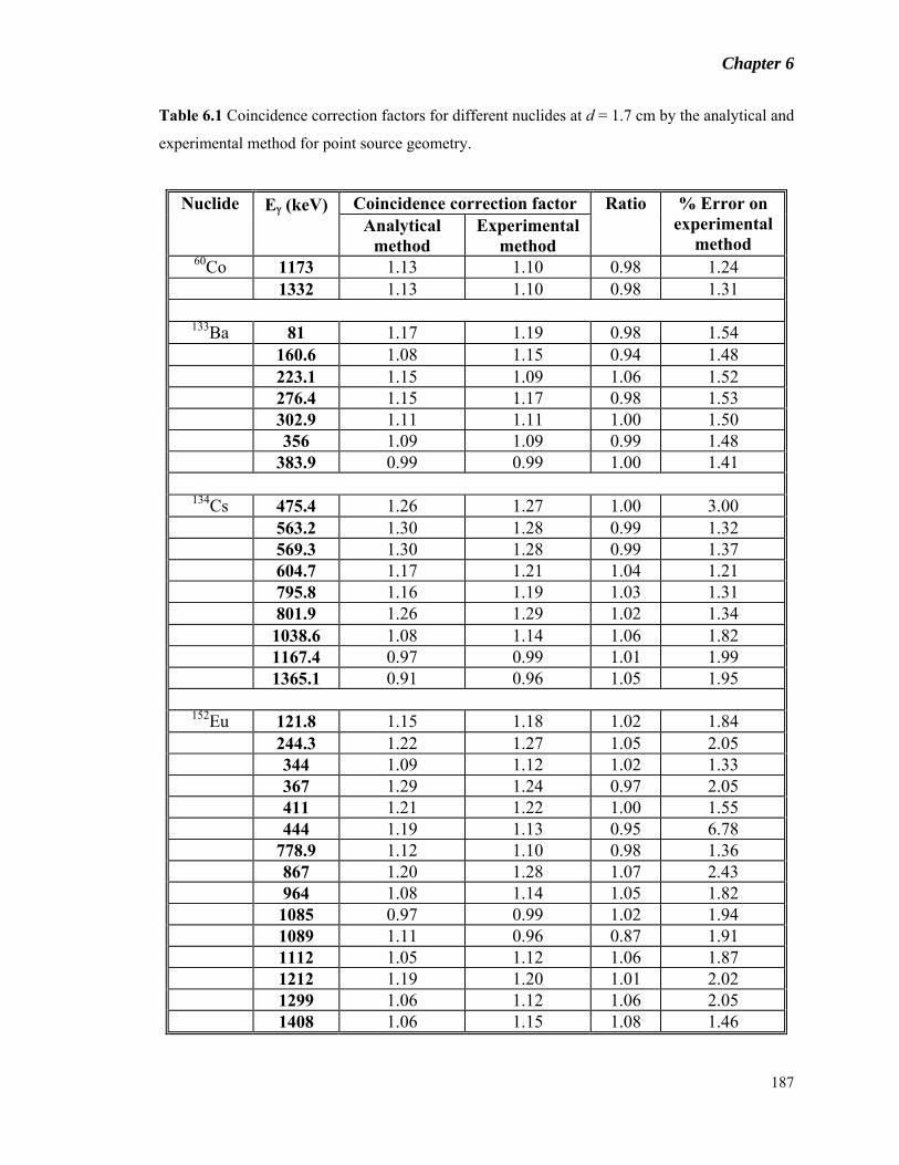
6.5.2 Validation of the Analytical Method

The analytical method was also verified by other method. Since MCNP is decay scheme

independent, the efficiency computed from MCNP for a monoenergetic source is free of

any coincidence summing whereas as shown in Figure 6.4, the efficiencies determined

experimentally are affected by coincidence summing effects. The true coincidence

summing correction factor as defined in equation 6.1 can be expressed as the ratio of

MCNP efficiency to the experimental efficiency:

(6.14)

The values of these experimental correction factors and their ratios with the correction

factors computed by analytical method are given in Table 6.1. It can be seen that for all

the nuclides, the factors from both the methods are matching within 1-5%. This validates

the analytical approach. Figure 6.5 shows the plot of efficiencies corrected for the true

coincidence summing correction factor obtained by the analytical method as a function of

energy at d = 1.7 cm. Here, practically all the points which were lying below the

efficiency curve before correction, are lying on the curve after correction giving rise to a

good efficiency curve after correction.

TCSMCNP efficiencyk

Experimental efficiency=

Chapter 6

187

Table 6.1 Coincidence correction factors for different nuclides at d = 1.7 cm by the analytical and

experimental method for point source geometry.

Coincidence correction factor Nuclide Eγ (keV) Analytical

method Experimental

method

Ratio % Error on experimental

method 60Co 1173 1.13 1.10 0.98 1.24

1332 1.13 1.10 0.98 1.31

133Ba 81 1.17 1.19 0.98 1.54 160.6 1.08 1.15 0.94 1.48 223.1 1.15 1.09 1.06 1.52 276.4 1.15 1.17 0.98 1.53 302.9 1.11 1.11 1.00 1.50 356 1.09 1.09 0.99 1.48 383.9 0.99 0.99 1.00 1.41

134Cs 475.4 1.26 1.27 1.00 3.00

563.2 1.30 1.28 0.99 1.32 569.3 1.30 1.28 0.99 1.37 604.7 1.17 1.21 1.04 1.21 795.8 1.16 1.19 1.03 1.31 801.9 1.26 1.29 1.02 1.34 1038.6 1.08 1.14 1.06 1.82 1167.4 0.97 0.99 1.01 1.99 1365.1 0.91 0.96 1.05 1.95

152Eu 121.8 1.15 1.18 1.02 1.84

244.3 1.22 1.27 1.05 2.05 344 1.09 1.12 1.02 1.33 367 1.29 1.24 0.97 2.05 411 1.21 1.22 1.00 1.55 444 1.19 1.13 0.95 6.78 778.9 1.12 1.10 0.98 1.36 867 1.20 1.28 1.07 2.43 964 1.08 1.14 1.05 1.82 1085 0.97 0.99 1.02 1.94 1089 1.11 0.96 0.87 1.91 1112 1.05 1.12 1.06 1.87 1212 1.19 1.20 1.01 2.02 1299 1.06 1.12 1.06 2.05 1408 1.06 1.15 1.08 1.46

Chapter 6

188

0 200 400 600 800 1000 1200 1400

0.01

0.02

0.03

0.04

0.05

0.06

0.07

0.08 152Eu 133Ba Noncoincident sources 60Co 134Cs 144Ce (FP) 106Ru (FP) 134Cs (FP) 137Cs (FP)Ef

ficie

ncy

Energy (keV)

Figure 6.5 Corrected Efficiencies as a function of gamma ray energy for point source geometry at

d = 1.7 cm. The solid line corresponds to the fourth order log-log fitting of efficiencies of

monoenergetic sources.

6.5.1 Application of the Method

A fission product sample in point source geometry was counted at d = 1.7 cm to get the

activity of different fission products such as 106Ru, 125Sb, 134Cs and 144Ce present in the

sample. The fission product spectrum is shown in Figure 6.6. Since these radionuclides

have gamma rays in cascade and at d = 1.7 cm, the true coincidence summing can be

appreciable, therefore TCS correction factors were obtained for these nuclides by both

the analytical and experimental method. These factors and their ratios are given in Table

6.2 and are found to match reasonably well. 137Cs was also present in the fission product

sample and as expected, its correction factor has been found to be close to unity. It can be

seen that there are practically no coincidence corrections for 125Sb and 144Ce. Since 125Sb

is a multi-gamma ray source, this is a very good candidate for efficiency calibration.

144Ce can also add to a point in efficiency curve in the low energy region which is very

Chapter 6

189

sensitive to the quality of fitting. The uncorrected and corrected efficiencies at gamma

ray energies of these radionuclides are also shown in Figure 6.4 and 6.5 respectively. The

corrected efficiencies at the gamma energies of 106Ru, 134Cs are found to lie on the fitted

curve of monoenergetic sources.

50 100 150 200 250 300 350 400 450 500

106

107

108

550 600 650 700 750 800 850 900 950 1000 1050 1100 1150

106

107

108

125 Sb

(463

keV

)

144 C

e(69

6 ke

V)

125 Sb

(428

keV

)

106 R

u(51

2 ke

V)

Cou

nts

Energy (keV)

Cou

nts

Energy (keV)

144 C

e(13

3 ke

V)

106 R

u(10

50 k

eV)

106 R

u(87

3 ke

V)

134 C

s(80

1 ke

V)

134 C

s(79

6 ke

V)

137 C

s(66

2 ke

V)

134 C

s(60

4 ke

V)10

6 Ru(

622

keV)

125 Sb

(636

keV

)

125 Sb

(176

keV

)

125 Sb

(601

keV

)

Figure 6.6 The gamma ray spectra of a fission product sample.

6.6 Coincidence summing correction for volumetric sources

Similarly, coincidence correction factors were obtained by both the methods for 5 ml

sources of 152Eu, 133Ba, 134Cs, 60Co, 22Na, 137Cs, 109Cd, 57Co, 203Hg, 65Zn and for nuclides

present in fission product solution. For this, these samples were counted at d = 10.3, 6.8,

4.4, and 2.0 cm respectively and the FEP efficiencies at these distances were obtained by

Chapter 6

190

using the determined disintegration rates of these sources. The FEP efficiency values of

all the sources at d = 10.3, 6.8, 4.4 and 2.0 cm are plotted in Figure 6.7(a-d) respectively.

The efficiencies from monoenergetic sources were fitted to a fourth order log – log

polynomial. The coincidence correction factors by analytical method were also obtained.

Here also, peak and total efficiencies required for the analytical method were calculated

by MCNP using the optimized detector geometry. As seen from Figure 6.7, for 5 ml

sources, even at d = 4.4 cm, the efficiencies obtained from the multi-gamma sources lie

on the fitted curves. This shows that even at d = 4.4 cm, the coincidence summing

corrections are negligible for 5 ml geometry. However, the coincidence summing effect is

more clearly seen at d = 2.0 cm where the efficiencies are not lying on the noncoincident

efficiency curve. This indicates the effect of true coincidence summing at this distance

and shows the need to obtain these correction factors. Table 6.3 and 6.4 lists the

coincidence correction factors obtained for the 5 ml mononuclide and fission product

sources by both the methods. The present method values are found to match within 1-5%

with the analytical method values. Figure 6.8 gives the FEP efficiencies corrected for

TCS obtained by the present method at d = 2.0 cm. All the points corresponding to multi-

energetic sources after correction lie on the FEP efficiency curve from monoenergetic

sources showing the validity of correction method for point and volumetric sources as

well.

Chapter 6

191

Table 6.2 Coincidence correction factors for nuclides present in fission product sample at d =

1.7 cm for point source geometry.

Coincidence correction factor Nuclide Eγ (keV) Analytical

method Experimental

method

Ratio

% Error on experimental

method 137Cs 661.6 1.00 1.02 0.98 1.21

144Ce 133.5 1.00 0.98 1.02 1.75

125Sb 176.3 1.01 0.98 1.03 1.51

427.9 1.00 1.02 0.99 3.28 463.4 1.00 0.92 1.08 1.40 600.6 1.00 1.02 0.98 1.40 635.9 1.00 1.09 0.91 1.71

106Ru 511.9 1.08 1.09 0.99 2.27

616.2 1.20 1.32 0.90 10.91 621.9 1.14 1.15 0.98 1.71 1050.3 1.13 1.11 1.02 2.03 1128 0.99 0.93 1.06 2.37

134Cs 563.2 1.30 1.30 1.00 1.56

569.3 1.30 1.30 0.99 1.50 604.7 1.17 1.20 0.97 1.24 795.8 1.16 1.14 1.01 1.34 801.9 1.26 1.28 0.99 1.66 1365.1 0.91 0.91 1.00 2.63

Chapter 6

192

0 200 400 600 800 1000 1200 1400

0.001

0.002

0.003

0.004

0.005

0.006

0.007


Effic

ienc

y

Energy (keV)0 200 400 600 800 1000 1200 1400

0.000

0.002

0.004

0.006

0.008

0.010

0.012


Effic

ienc

y

Energy (keV)

0 200 400 600 800 1000 1200 1400

0.005

0.010

0.015

0.020


Effi

cien

cy

Energy (keV)0 200 400 600 800 1000 1200 1400

0.01

0.02

0.03

0.04

0.05

0.06


Effic

ienc

y

Energy (keV)

Figure 6.7 Efficiencies as a function of gamma ray energy for point source geometry at sample-

to-detector distances, d = (a) 10.3 cm, (b) 6.8 cm, (c) 4.4 cm and (d) 2.0 cm. The solid line

corresponds to the fourth order log-log fitting of efficiencies of monoenergetic sources. The

nuclides marked with FP in the figure shows the nuclides present in the fission product sample.

(a) (b)

(c) (d)

Chapter 6

193

0 200 400 600 800 1000 1200 1400

0.01

0.02

0.03

0.04

0.05


Effic

ienc

y

Energy (keV)

Figure 6.8 Corrected efficiencies as a function of gamma ray energy for 5 ml geometry at

sample-to-detector distances, d = 2.0 cm. The solid line corresponds to the fourth order log-log

fitting of efficiencies of monoenergetic sources. The nuclides marked with FP in the figure shows

the nuclides present in the fission product sample.

Chapter 6

194

Table 6.3 Coincidence correction factors for different nuclides at d = 2.0 cm by the analytical and

experimental method for 5 ml source geometry.

Coincidence correction factor Nuclide Eγ

(keV) Analytical method

Experimental method

Ratio % Error on

present method

60Co 1173 1.11 1.13 1.02 1.25 1332 1.11 1.13 1.02 1.32

152Eu 121.8 1.13 1.13 1.00 1.63 244.3 1.18 1.17 0.99 2.02 344 1.08 1.05 0.97 1.30 444 1.16 1.14 0.99 6.79 778.9 1.11 1.06 0.96 1.30 867 1.17 1.22 1.04 2.45 964 1.07 1.09 1.02 1.79 1085 0.98 0.99 1.01 1.95 1089 1.10 1.00 0.91 2.14 1112 1.04 1.08 1.04 1.88 1212 1.16 1.18 1.02 2.40 1408 1.05 1.08 1.03 1.55

133Ba 81 1.11 1.15 1.04 1.38 160.6 1.01 1.06 1.06 1.89 223.1 1.02 1.14 1.12 1.93 276.4 1.06 1.12 1.06 1.18 302.9 1.03 1.07 1.04 1.15 356 1.02 1.05 1.02 1.13 383.9 0.95 0.97 1.02 1.18

134Cs 475.4 1.22 1.11 0.91 2.99 563.2 1.25 1.17 0.94 1.26 569.3 1.25 1.14 0.91 1.30 604.7 1.14 1.08 0.94 1.13 795.8 1.13 1.09 0.96 1.20 801.9 1.22 1.13 0.93 1.24 1038.6 1.06 1.05 0.98 1.83 1167.4 0.97 0.92 0.94 2.01 1365.1 0.92 0.87 0.95 2.00

Chapter 6

195

Table 6.4 Coincidence correction factors for nuclides present in fission product sample at d = 2.0

cm for 5 ml geometry.

Coincidence correction factor Nuclide Eγ

(keV) Analytical method

Experimental method

Ratio % Error on present method

137Cs 661.6 1.00 1.01 1.01 1.03

144Ce 133.5 1.00 1.01 0.99 1.49

125Sb 176.3 1.01 1.10 1.09 1.44 427.9 1.00 0.94 0.93 3.28 463.4 1.00 0.93 0.93 1.49 600.6 1.00 0.99 0.99 1.45 635.9 1.00 1.00 1.00 1.80

106Ru 511.9 1.07 1.08 1.01 2.24

616.2 1.17 1.29 1.11 10.92 621.9 1.12 1.15 1.03 1.66 1050.3 1.11 1.38 1.25 2.05 1128 0.99 1.03 1.03 2.55 1562 0.81 0.86 1.07 3.53

134Cs 563.2 1.25 1.24 0.99 2.06

569.3 1.25 1.17 0.94 1.97 604.7 1.14 1.1 0.96 1.58 795.8 1.13 1.1 0.97 1.67 801.9 1.22 1.2 0.98 2.11 1365.1 0.92 0.9 0.98 3.53

6.7 Conclusion

Coincidence summing becomes very important at closer sample-to-detector geometry.

Correction factors as high as 30% have been observed. MCNP calculated FEP and total

efficiencies with optimized detector geometry can be effectively used to obtain

coincidence correction factors using the analytical approach.

true coincidence summing corrections -...

Documents