true 4d image denoising on the gpu - diva...

True 4D Image Denoising on the GPU

Anders Eklund, Mats Andersson and Hans Knutsson

Linköping University Post Print

N.B.: When citing this work, cite the original article.

Original Publication:

Anders Eklund, Mats Andersson and Hans Knutsson, True 4D Image Denoising on the GPU,

2011, International Journal of Biomedical Imaging, (2011).

http://dx.doi.org/10.1155/2011/952819

Copyright: Hindawi Publishing Corporation

http://www.hindawi.com/

Postprint available at: Linköping University Electronic Press

http://urn.kb.se/resolve?urn=urn:nbn:se:liu:diva-69678

http://dx.doi.org/10.1155/2011/952819

http://www.hindawi.com/

http://urn.kb.se/resolve?urn=urn:nbn:se:liu:diva-69678

Hindawi Publishing CorporationInternational Journal of Biomedical ImagingVolume 2011, Article ID 952819, 16 pagesdoi:10.1155/2011/952819

Research Article

True 4D Image Denoising on the GPU

Anders Eklund,1, 2 Mats Andersson,1, 2 and Hans Knutsson1, 2

1 Division of Medical Informatics, Department of Biomedical Engineering, Linkoping University, Linkoping, Sweden2 Center for Medical Image Science and Visualization (CMIV), Linkoping University, Linkoping, Sweden

Correspondence should be addressed to Anders Eklund, [email protected]

Received 31 March 2011; Revised 23 June 2011; Accepted 24 June 2011

Academic Editor: Khaled Z. Abd-Elmoniem

Copyright © 2011 Anders Eklund et al. This is an open access article distributed under the Creative Commons Attribution License,which permits unrestricted use, distribution, and reproduction in any medium, provided the original work is properly cited.

The use of image denoising techniques is an important part of many medical imaging applications. One common application is toimprove the image quality of low-dose (noisy) computed tomography (CT) data. While 3D image denoising previously has beenapplied to several volumes independently, there has not been much work done on true 4D image denoising, where the algorithmconsiders several volumes at the same time. The problem with 4D image denoising, compared to 2D and 3D denoising, is that thecomputational complexity increases exponentially. In this paper we describe a novel algorithm for true 4D image denoising, basedon local adaptive filtering, and how to implement it on the graphics processing unit (GPU). The algorithm was applied to a 4D CTheart dataset of the resolution 512 × 512 × 445 × 20. The result is that the GPU can complete the denoising in about 25 minutesif spatial filtering is used and in about 8 minutes if FFT-based filtering is used. The CPU implementation requires several days ofprocessing time for spatial filtering and about 50 minutes for FFT-based filtering. The short processing time increases the clinicalvalue of true 4D image denoising significantly.

1. Introduction

Image denoising is commonly used in medical imaging inorder to help medical doctors to see abnormalities in theimages. Image denoising was first applied to 2D images[1–3] and then extended to 3D data [4–6], 3D data caneither be collected as several 2D images over time or as one3D volume. A number of medical imaging modalities (e.g.,computed tomography (CT), ultrasound (US) and magneticresonance imaging (MRI)) now provide the possibility tocollect 4D data, that is, time-resolved volume data. Thismakes it possible to, for example, examine what parts ofthe brain that are active during a certain task (functionalmagnetic resonance imaging (fMRI)). While 4D CT datamakes it possible to see the heart beat in 3D, the drawbackis that a lower amount of X-ray exposure has to be used for4D CT data collection, compared to 3D CT data collection, inorder to not harm the patient. When the amount of exposureis decreased, the amount of noise in the data increasessignificantly.

Three-dimensional image denoising has previously beenapplied to several time points independently, but there hasnot been much work done on true 4D image denoisingwhere the algorithm considers several volumes at the same

time (and not a single volume at a time). Montagnat et al.[7] applied 4D anisotropic diffusion filtering to ultrasoundvolumes and Jahanian et al. [8] applied 4D wavelet denoisingto diffusion tensor MRI data. For CT data, it can be extrabeneficial to use the time dimension in the denoising, assome of the reconstruction artefacts vary with time. It isthereby possible to remove these artefacts by taking fulladvantage of the 4D data. While true 4D image denoisingis very powerful, the drawback is that the processing timeincreases exponentially with respect to dimensionality.

The rapid development of graphics processing units(GPUs) has resulted in that many algorithms in the medicalimaging domain have been implemented on the GPU, inorder to save time and to be able to apply more advancedanalysis. To give an example of the rapid GPU development,a comparison of three consumer graphic cards from Nvidiais given in Table 1. The time frame between each GPUgeneration is 2-3 years. Some examples of fields in medicalimaging that have taken advantage of the computationalpower of the GPU are image registration [9–13], imagesegmentation [14–16] and fMRI analysis [17–20].

In the area of image denoising, some algorithms have alsobeen implemented on the GPU. Already in 2001 Rumpf and

2 International Journal of Biomedical Imaging

Table 1: Comparison between three Nvidia GPUs, from three different generations, in terms of processor cores, memory bandwidth, sizeof shared memory, cache memory, and number of registers; MP stands for multiprocessor and GB/s stands for gigabytes per second. For theGTX 580, the user can for each kernel choose to use 48 KB of shared memory and 16 KB of L1 cache or vice versa.

Property/GPU 9800 GT GTX 285 GTX 580

Number of processor cores 112 240 512

Normal size of global memory 512 MB 1024 MB 1536 MB

Global memory bandwidth 57.6 GB/s 159.0 GB/s 192.4 GB/s

Constant memory 64 KB 64 KB 64 KB

Shared memory per MP 16 KB 16 KB 48/16 KB

Float registers per MP 8192 16384 32768

L1 cache per MP None None 16/48 KB

L2 cache None None 768 KB

Strzodka [21] described how to apply anisotropic diffusion[3] on the GPU. Howison [22] made a comparison betweendifferent GPU implementations of anisotropic diffusion andbilateral filtering for 3D data. Su and Xu [23] in 2010 pro-posed how to accelerate wavelet-based image denoising byusing the GPU. Zhang et al. [24] describe GPU-based imagemanipulation and enhancement techniques for dynamicvolumetric medical image visualization, but enhancement inthis case refers to enhancement of the visualization, and notof the 4D data. Recently, the GPU has been used for real-time image denoising. In 2007, Chen et al. [25] used bilateralfiltering [26] on the GPU for real-time edge-aware imageprocessing. Fontes et al. [27] in 2011 used the GPU for real-time denoising of ultrasound data and Goossens et al. [28]in 2010 managed to run the commonly used nonlocal meansalgorithm [29] in real time.

To our knowledge, there has not been any work doneabout true 4D image denoising on the GPU. In this work wetherefore present a novel algorithm, based on local adaptivefiltering, for 4D denoising and describe how to implementit on the GPU, in order to decrease the processing time andthereby significantly increase the clinical value.

2. Methods

In this section, the algorithm that is used for true 4D imagedenoising will be described.

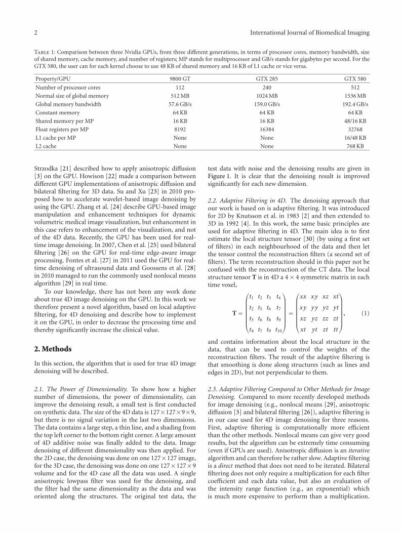
2.1. The Power of Dimensionality. To show how a highernumber of dimensions, the power of dimensionality, canimprove the denoising result, a small test is first conductedon synthetic data. The size of the 4D data is 127×127×9×9,but there is no signal variation in the last two dimensions.The data contains a large step, a thin line, and a shading fromthe top left corner to the bottom right corner. A large amountof 4D additive noise was finally added to the data. Imagedenoising of different dimensionality was then applied. Forthe 2D case, the denoising was done on one 127×127 image,for the 3D case, the denoising was done on one 127×127×9volume and for the 4D case all the data was used. A singleanisotropic lowpass filter was used for the denoising, andthe filter had the same dimensionality as the data and wasoriented along the structures. The original test data, the

test data with noise and the denoising results are given inFigure 1. It is clear that the denoising result is improvedsignificantly for each new dimension.

2.2. Adaptive Filtering in 4D. The denoising approach thatour work is based on is adaptive filtering. It was introducedfor 2D by Knutsson et al. in 1983 [2] and then extended to3D in 1992 [4]. In this work, the same basic principles areused for adaptive filtering in 4D. The main idea is to firstestimate the local structure tensor [30] (by using a first setof filters) in each neighbourhood of the data and then letthe tensor control the reconstruction filters (a second set offilters). The term reconstruction should in this paper not beconfused with the reconstruction of the CT data. The localstructure tensor T is in 4D a 4× 4 symmetric matrix in eachtime voxel,

T =

⎛⎜⎜⎜⎜⎜⎜⎝

t1 t2 t3 t4

t2 t5 t6 t7

t3 t6 t8 t9

t4 t7 t9 t10

⎞⎟⎟⎟⎟⎟⎟⎠=

⎛⎜⎜⎜⎜⎜⎜⎝

xx xy xz xt

xy yy yz yt

xz yz zz zt

xt yt zt tt

⎞⎟⎟⎟⎟⎟⎟⎠

, (1)

and contains information about the local structure in thedata, that can be used to control the weights of thereconstruction filters. The result of the adaptive filtering isthat smoothing is done along structures (such as lines andedges in 2D), but not perpendicular to them.

2.3. Adaptive Filtering Compared to Other Methods for ImageDenoising. Compared to more recently developed methodsfor image denoising (e.g., nonlocal means [29], anisotropicdiffusion [3] and bilateral filtering [26]), adaptive filtering isin our case used for 4D image denoising for three reasons.First, adaptive filtering is computationally more efficientthan the other methods. Nonlocal means can give very goodresults, but the algorithm can be extremely time consuming(even if GPUs are used). Anisotropic diffusion is an iterativealgorithm and can therefore be rather slow. Adaptive filteringis a direct method that does not need to be iterated. Bilateralfiltering does not only require a multiplication for each filtercoefficient and each data value, but also an evaluation ofthe intensity range function (e.g., an exponential) whichis much more expensive to perform than a multiplication.

International Journal of Biomedical Imaging 3

Original Degraded 2D Denoising 3D Denoising 4D Denoising

(1) (2) (3) (4) (5)

Figure 1: (1) Original test image without noise. There is a large step in the middle, a bright thin line and a shading from the top left cornerto the bottom right corner. (2) Original test image with a lot of noise. The step is barely visible, while it is impossible to see the line or theshading. (3) Resulting image after 2D denoising. The step is almost visible and it is possible to see that the top left corner is brighter than thebottom right corner. (4) Resulting image after 3D denoising. Now the step and the shading are clearly visible, but not the line. (5) Resultingimage after 4D denoising. Now all parts of the image are clearly visible.

Second, the tuning of the parameters is for our denoisingalgorithm rather easy to understand and to explore. Whena first denoising result has been obtained, it is often obvioushow to change the parameters to improve the result. This isnot always the case for other methods. Third, the adaptivefiltering approach has been proven to be very robust (it isextremely seldom that a strange result is obtained). Adaptivefiltering has been used for 2D image denoising in commercialclinical software for over 20 years and a recent 3D study [31]proves its potential, robustness, and clinical acceptance. Thenonlocal means algorithm only works if the data containsseveral neighbourhoods with similar properties.

2.4. Estimating the Local Structure Tensor Using QuadratureFilters. The local structure tensor can, for example, beestimated by using quadrature filters [5, 30]. QuadraturefiltersQ are zero in one half of the frequency domain (definedby the direction of the filter) and can be expressed as twopolar separable functions, one radial function R and onedirectional function D,

Q(u) = R(‖u‖)D(u), (2)

where u is the frequency variable. The radial function is alognormal function

R(‖u‖) = exp(C ln2

(‖u‖u0

)), C = −4

B2 ln(2), (3)

where u0 is the centre frequency of the filter and B is thebandwidth (in octaves). The directional function dependson the angle θ between the filter direction vector n and thenormalized frequency coordinate vector u as cos(θ)2,

D(u) =⎧⎪⎨⎪⎩

(uT n

)2, uT n > 0,

0, otherwise.(4)

Quadrature filters are Cartesian nonseparable and complexvalued in the spatial domain, the real part is even and in 2Dacts as a line detector, while the imaginary part is odd andin 2D acts as an edge detector. In 3D, the even and odd filterscorrespond to a plane detector and a 3D edge detector. In 4D,

the plane and 3D edge may in addition be time varying. Thecomplex-valued filter response q is an estimate of a bandpassfiltered version of the analytical signal with magnitude A andphase φ,

q = A(cos(φ)

+ i · sin(φ)) = Aeiφ. (5)

The tensor is calculated by multiplying the magnitude of thequadrature filter response qk with the outer product of thefilter direction vector nk and then summing the result overall filters k,

T =Nf∑

k=1

∣∣qk∣∣(c1nknT

k − c2I)

, (6)

where c1 and c2 are scalar constants that depend on thedimensionality of the data [5, 30], Nf is the number ofquadrature filters and I is the identity matrix. The resultingtensor is phase invariant, as the magnitude of the quadraturefilter response is invariant to the type of local neighbourhood(e.g., in 2D bright lines, dark lines, dark to bright edges,etc.). This is in contrast to when the local structure tensoris estimated by using gradient operators, such as Sobel filters.

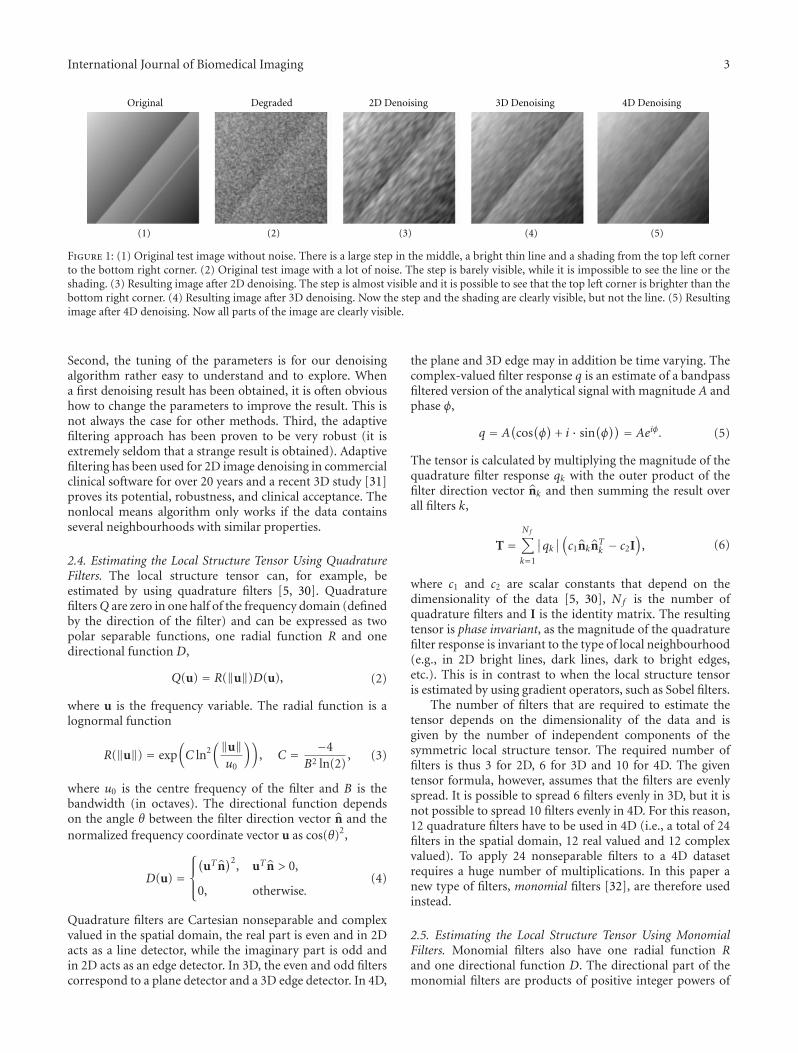
The number of filters that are required to estimate thetensor depends on the dimensionality of the data and isgiven by the number of independent components of thesymmetric local structure tensor. The required number offilters is thus 3 for 2D, 6 for 3D and 10 for 4D. The giventensor formula, however, assumes that the filters are evenlyspread. It is possible to spread 6 filters evenly in 3D, but it isnot possible to spread 10 filters evenly in 4D. For this reason,12 quadrature filters have to be used in 4D (i.e., a total of 24filters in the spatial domain, 12 real valued and 12 complexvalued). To apply 24 nonseparable filters to a 4D datasetrequires a huge number of multiplications. In this paper anew type of filters, monomial filters [32], are therefore usedinstead.

2.5. Estimating the Local Structure Tensor Using MonomialFilters. Monomial filters also have one radial function Rand one directional function D. The directional part of themonomial filters are products of positive integer powers of


the components of the frequency variable u. The monomialfilter matrices of order one, F1, and two, F2, are in thefrequency domain defined as

F1,n = R(‖u‖)un, F2,mn = R(‖u‖)umun. (7)

The monomial filters are first described for 2D and thengeneralized to 4D.

2.5.1. Monomial Filters in 2D. In 2D, the frequency variableis in this work defined as u = [u v]T . The directional part offirst-order monomial filters are x, y in the spatial domain andu, v in the frequency domain. Two-dimensional monomialfilters of the first-order are given in Figure 2. The directionalpart of second-order monomial filters are xx, xy, yy in thespatial domain and uu,uv, vv in the frequency domain. Twodimensional monomial filters of the second order are givenin Figure 3.

The monomial filter response matrices Q are eithercalculated by convolution in the spatial domain or bymultiplication in the frequency domain. For a simple signalwith phase θ (e.g., s(x) = A cos(uTx + θ)); the monomialfilter response matrices of order one and two can be writtenas

Q1 = −iA sin(θ)[uv]T ,

Q2 = A cos(θ)

⎛⎝uu uv

uv vv

⎞⎠.

(8)

The first-order products are odd functions and are therebyrelated to the odd sine function, the second order productsare even functions and are thereby related to the even cosinefunction (note the resemblance with quadrature filters thathave one even real part and one odd imaginary part). Byusing the fact that u2 + v2 = 1, the outer products of thefilter response matrices give

Q1Q1T = sin2(θ)|A|2

⎛⎝uu uv

uv vv

⎞⎠,

Q2Q2T = cos2(θ)|A|2

⎛⎝uu uv

uv vv

⎞⎠.

(9)

The local structure tensor T is then calculated as

T = Q1Q1T + Q2Q2

T = |A|2⎛⎝uu uv

uv vv

⎞⎠. (10)

From this expression, it is clear that the estimated tensor,as previously, is phase invariant as the square of one oddpart and the square of one even part are combined. Forinformation about how to calculate the tensor for higher-order monomials, see our recent work [32].

2.5.2. Monomial Filters in 4D. A total of 14 nonseparable 4Dmonomial filters (4 odd of the first-order (x, y, z, t) and 10even of the second-order (xx, xy, xz, xt, yy, yz, yt, zz, zt, tt))

Frequency domainu v

(a)

Spatial domainx y

(b)

Figure 2: (a) Two-dimensional monomial filters (u, v), of the firstorder, in the frequency domain. Green indicates positive real valuesand red indicates negative real values. The black lines are isocurves.(b) Two-dimensional monomial filters (x, y), of the first order, inthe spatial domain. Yellow indicates positive imaginary values, andblue indicates negative imaginary values. Note that these filters areodd and imaginary.

with a spatial support of 7 × 7 × 7 × 7 time voxels areapplied to the CT volumes. The filters have a lognormalradial function with centre frequency 3π/5 and a bandwidthof 2.5 octaves. The filter kernels were optimized with respectto ideal frequency response, spatial locality, and expectedsignal-to-noise ratio [5, 33].

By using equation (10) for the 4D case, and replacingthe frequency variables with the monomial filter responses,the 10 components of the structure tensor are calculatedaccording to

t1 = f r1 · f r1 + f r5 · f r5 + f r6 · f r6 + f r7 · f r7

+ f r8 · f r8,


+ f r8 · f r11,


+ f r8 · f r13,


+ f r8 · f r14,


+ f r11 · f r11,


Frequency domainuu uv vv

(a)

Spatial domainxx xy yy

(b)

Figure 3: (a) Two-dimensional monomial filters (uu,uv, v), of the second order, in the frequency domain. Green indicates positive realvalues, and red indicates negative real values. The black lines are isocurves. (b) Two-dimensional monomial filters (xx, xy, yy), of the secondorder, in the spatial domain. Green indicates positive real values, and red indicates negative real values. Note that these filters are even andreal.


+ f r11 · f r13,


+ f r11 · f r14,


+ f r13 · f r13,


+ f r13 · f r14,


+ f r14 · f r14,

(11)

where f rk denotes the filter response for monomial filter k.The first term relates to Q1Q1

T , and the rest of the termsrelate to Q2Q2

T , in total Q1Q1T + Q2Q2

T .If monomial filters are used instead of quadrature filters,

the required number of 4D filters is thus decreased from 24 to14. Another advantage is that the monomial filters require asmaller spatial support, which makes it easier to preserve de-tails and contrast in the processing. A smaller spatial support

also results in a lower number of filter coefficients, whichdecreases the processing time.

2.6. The Control Tensor. When the local structure tensor Thas been estimated, it is then mapped to a control tensor C,by mapping the magnitude (energy) and the isotropy of thetensor. The purpose of this mapping is to further improve thedenoising. For 2D and 3D image denoising, this mapping canbe done by first calculating the eigenvalues and eigenvectorsof the structure tensor in each element of the data. Themapping is first described for 2D and then for 4D.

2.6.1. Mapping the Magnitude of the Tensor in 2D. In the 2Dcase, the magnitude γ0 of the tensor is calculated as

γ0 =√λ2

1 + λ22, (12)

where λ1 and λ2 are the two eigenvalues. The magnitude γ0 isnormalized to vary between 0 and 1 and is then mapped to γwith a so-called M-function according to

γ =⎛⎝ γ

β0

γα + β

0 + σ β

⎞⎠, (13)

where α, β, and σ are parameters that are used to controlthe mapping. The σ variable is directly proportional to thesignal-to-noise (SNR) ratio of the data and acts as a soft


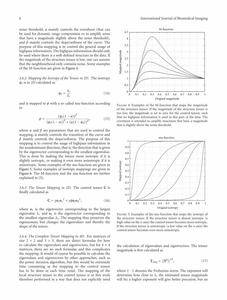
noise threshold, α mainly controls the overshoot (that canbe used for dynamic range compression or to amplify areasthat have a magnitude slightly above the noise threshold),and β mainly controls the slope/softness of the curve. Thepurpose of this mapping is to control the general usage ofhighpass information. The highpass information should onlybe used where there is a well-defined structure in the data. Ifthe magnitude of the structure tensor is low, one can assumethat the neighbourhood only contains noise. Some examplesof the M-function are given in Figure 4.

2.6.2. Mapping the Isotropy of the Tensor in 2D. The isotropyφ0 is in 2D calculated as

φ0 = λ2

λ1(14)

and is mapped to φ with a so called mu-function accordingto

φ =(φ0(1− α)

)β(φ0(1− α)

)β +(α(1− φ0

))β , (15)

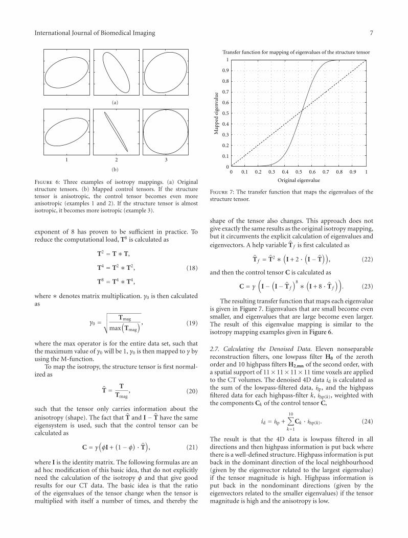
where α and β are parameters that are used to control themapping, α mainly controls the transition of the curve andβ mainly controls the slope/softness. The purpose of thismapping is to control the usage of highpass information inthe nondominant direction, that is, the direction that is givenby the eigenvector corresponding to the smallest eigenvalue.This is done by making the tensor more isotropic if it isslightly isotropic, or making it even more anisotropic if it isanisotropic. Some examples of the mu-function are given inFigure 5. Some examples of isotropy mappings are given inFigure 6. The M-function and the mu-function are furtherexplained in [5].

2.6.3. The Tensor Mapping in 2D. The control tensor C isfinally calculated as

C = γe1e1T + γφe2e2

T , (16)

where e1 is the eigenvector corresponding to the largesteigenvalue λ1 and e2 is the eigenvector corresponding tothe smallest eigenvalue λ2. The mapping thus preserves theeigensystem, but changes the eigenvalues and thereby theshape of the tensor.

2.6.4. The Complete Tensor Mapping in 4D. For matrices ofsize 2 × 2 and 3 × 3, there are direct formulas for howto calculate the eigenvalues and eigenvectors, but for 4 × 4matrices, there are no such formulas and this complicatesthe mapping. It would of course be possible to calculate theeigenvalues and eigenvectors by other approaches, such asthe power iteration algorithm, but this would be extremelytime consuming as the mapping to the control tensorhas to be done in each time voxel. The mapping of thelocal structure tensor to the control tensor is in this worktherefore performed in a way that does not explicitly need

0 0.1 0.2 0.3 0.4 0.5 0.6 0.7 0.8 0.9 10

0.5

1

1.5

2

2.5

3

3.5

4

4.5M-function

Original magnitude

Map

ped

mag

nit

ude

Figure 4: Examples of the M-function that maps the magnitudeof the structure tensor. If the magnitude of the structure tensor istoo low, the magnitude is set to zero for the control tensor, suchthat no highpass information is used in this part of the data. Theovershoot is intended to amplify structures that have a magnitudethat is slightly above the noise threshold.

0

0.1

0.2

0.3

0.4

0.5

0.6

0.7

0.8

0.9

1mu-function

Original isotropy

Map

ped

isot

ropy

0 0.1 0.2 0.3 0.4 0.5 0.6 0.7 0.8 0.9 1

Figure 5: Examples of the mu-function that maps the isotropy ofthe structure tensor. If the structure tensor is almost isotropic (ahigh value on the x-axis) the control tensor becomes more isotropic.If the structure tensor is anisotropic (a low value on the x-axis) thecontrol tensor becomes even more anisotropic.

the calculation of eigenvalues and eigenvectors. The tensormagnitude is first calculated as

Tmag =∥∥T8

∥∥1/8, (17)

where ‖ · ‖ denotes the Frobenius norm. The exponent willdetermine how close to λ1 the estimated tensor magnitudewill be; a higher exponent will give better precision, but an


(a)

1 2 3

(b)

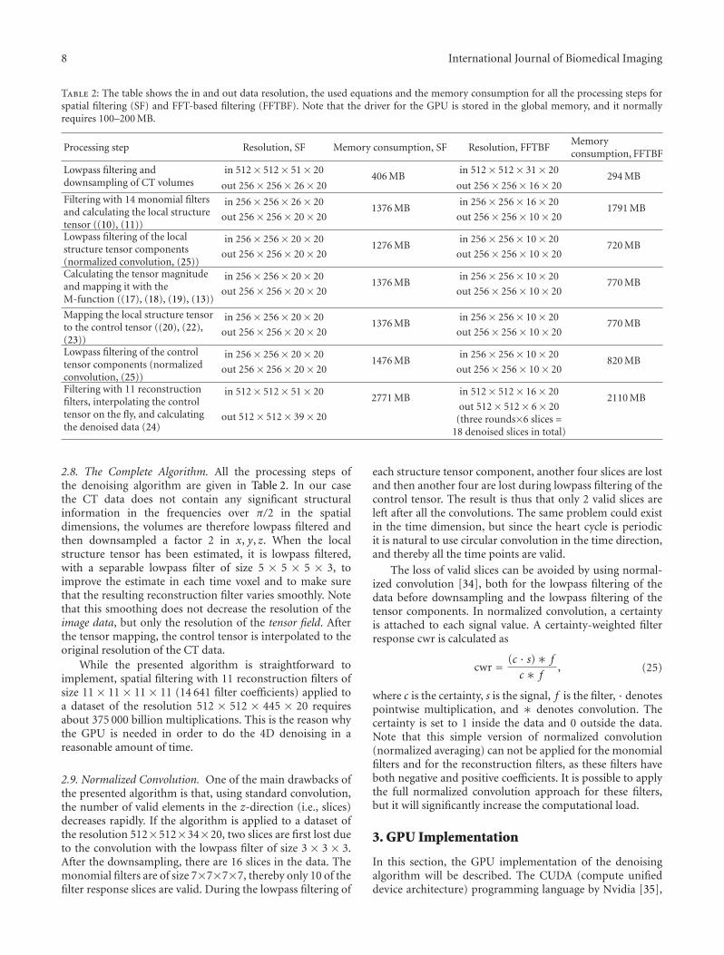
Figure 6: Three examples of isotropy mappings. (a) Originalstructure tensors. (b) Mapped control tensors. If the structuretensor is anisotropic, the control tensor becomes even moreanisotropic (examples 1 and 2). If the structure tensor is almostisotropic, it becomes more isotropic (example 3).

exponent of 8 has proven to be sufficient in practice. Toreduce the computational load, T8 is calculated as

T2 = T∗ T,

T4 = T2 ∗ T2,

T8 = T4 ∗ T4,

(18)

where ∗ denotes matrix multiplication. γ0 is then calculatedas

γ0 =√√√√ Tmag

max(

Tmag

) , (19)

where the max operator is for the entire data set, such thatthe maximum value of γ0 will be 1, γ0 is then mapped to γ byusing the M-function.

To map the isotropy, the structure tensor is first normal-ized as

T = TTmag

, (20)

such that the tensor only carries information about theanisotropy (shape). The fact that T and I − T have the sameeigensystem is used, such that the control tensor can becalculated as

C = γ(φI +

(1− φ

) · T)

, (21)

where I is the identity matrix. The following formulas are anad hoc modification of this basic idea, that do not explicitlyneed the calculation of the isotropy φ and that give goodresults for our CT data. The basic idea is that the ratioof the eigenvalues of the tensor change when the tensor ismultiplied with itself a number of times, and thereby the

0

0.1

0.2

0.3

0.4

0.5

0.6

0.7

0.8

0.9

1

Transfer function for mapping of eigenvalues of the structure tensor

Original eigenvalue

Map

ped

eige

nval

ue

0 0.1 0.2 0.3 0.4 0.5 0.6 0.7 0.8 0.9 1

Figure 7: The transfer function that maps the eigenvalues of thestructure tensor.

shape of the tensor also changes. This approach does notgive exactly the same results as the original isotropy mapping,but it circumvents the explicit calculation of eigenvalues andeigenvectors. A help variable T f is first calculated as

T f = T2 ∗(

I + 2 ·(

I− T))

, (22)

and then the control tensor C is calculated as

C = γ(

I−(

I− T f

)8 ∗(

I + 8 · T f

)). (23)

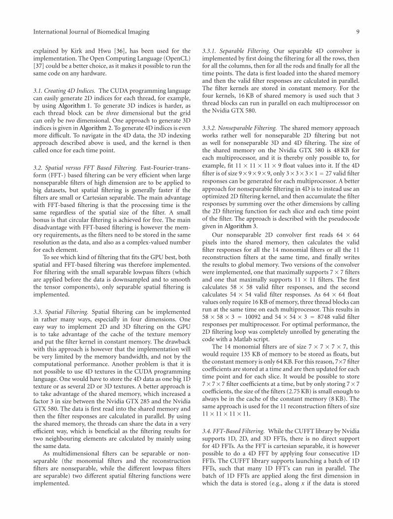
The resulting transfer function that maps each eigenvalueis given in Figure 7. Eigenvalues that are small become evensmaller, and eigenvalues that are large become even larger.The result of this eigenvalue mapping is similar to theisotropy mapping examples given in Figure 6.

2.7. Calculating the Denoised Data. Eleven nonseparablereconstruction filters, one lowpass filter H0 of the zerothorder and 10 highpass filters H2,mn of the second order, witha spatial support of 11× 11× 11× 11 time voxels are appliedto the CT volumes. The denoised 4D data id is calculated asthe sum of the lowpass-filtered data, ilp, and the highpassfiltered data for each highpass-filter k, ihp(k), weighted withthe components Ck of the control tensor C,

id = ilp +10∑

k=1

Ck · ihp(k). (24)

The result is that the 4D data is lowpass filtered in alldirections and then highpass information is put back wherethere is a well-defined structure. Highpass information is putback in the dominant direction of the local neighbourhood(given by the eigenvector related to the largest eigenvalue)if the tensor magnitude is high. Highpass information isput back in the nondominant directions (given by theeigenvectors related to the smaller eigenvalues) if the tensormagnitude is high and the anisotropy is low.


Table 2: The table shows the in and out data resolution, the used equations and the memory consumption for all the processing steps forspatial filtering (SF) and FFT-based filtering (FFTBF). Note that the driver for the GPU is stored in the global memory, and it normallyrequires 100–200 MB.

Processing step Resolution, SF Memory consumption, SF Resolution, FFTBFMemoryconsumption, FFTBF

Lowpass filtering anddownsampling of CT volumes

in 512× 512× 51× 20406 MB

in 512× 512× 31× 20294 MB

out 256× 256× 26× 20 out 256× 256× 16× 20Filtering with 14 monomial filtersand calculating the local structuretensor ((10), (11))

in 256× 256× 26× 201376 MB

in 256× 256× 16× 201791 MB

out 256× 256× 20× 20 out 256× 256× 10× 20

Lowpass filtering of the localstructure tensor components(normalized convolution, (25))

in 256× 256× 20× 201276 MB

in 256× 256× 10× 20720 MB

out 256× 256× 20× 20 out 256× 256× 10× 20

Calculating the tensor magnitudeand mapping it with theM-function ((17), (18), (19), (13))

in 256× 256× 20× 201376 MB

in 256× 256× 10× 20770 MB

out 256× 256× 20× 20 out 256× 256× 10× 20

Mapping the local structure tensorto the control tensor ((20), (22),(23))

in 256× 256× 20× 201376 MB

in 256× 256× 10× 20770 MB

out 256× 256× 20× 20 out 256× 256× 10× 20

Lowpass filtering of the controltensor components (normalizedconvolution, (25))

in 256× 256× 20× 201476 MB

in 256× 256× 10× 20820 MB

out 256× 256× 20× 20 out 256× 256× 10× 20

Filtering with 11 reconstructionfilters, interpolating the controltensor on the fly, and calculatingthe denoised data (24)

in 512× 512× 51× 202771 MB

in 512× 512× 16× 202110 MB

out 512× 512× 39× 20out 512× 512× 6× 20

(three rounds×6 slices =18 denoised slices in total)

2.8. The Complete Algorithm. All the processing steps ofthe denoising algorithm are given in Table 2. In our casethe CT data does not contain any significant structuralinformation in the frequencies over π/2 in the spatialdimensions, the volumes are therefore lowpass filtered andthen downsampled a factor 2 in x, y, z. When the localstructure tensor has been estimated, it is lowpass filtered,with a separable lowpass filter of size 5 × 5 × 5 × 3, toimprove the estimate in each time voxel and to make surethat the resulting reconstruction filter varies smoothly. Notethat this smoothing does not decrease the resolution of theimage data, but only the resolution of the tensor field. Afterthe tensor mapping, the control tensor is interpolated to theoriginal resolution of the CT data.

While the presented algorithm is straightforward toimplement, spatial filtering with 11 reconstruction filters ofsize 11 × 11 × 11 × 11 (14 641 filter coefficients) applied toa dataset of the resolution 512 × 512 × 445 × 20 requiresabout 375 000 billion multiplications. This is the reason whythe GPU is needed in order to do the 4D denoising in areasonable amount of time.

2.9. Normalized Convolution. One of the main drawbacks ofthe presented algorithm is that, using standard convolution,the number of valid elements in the z-direction (i.e., slices)decreases rapidly. If the algorithm is applied to a dataset ofthe resolution 512×512×34×20, two slices are first lost dueto the convolution with the lowpass filter of size 3 × 3 × 3.After the downsampling, there are 16 slices in the data. Themonomial filters are of size 7×7×7×7, thereby only 10 of thefilter response slices are valid. During the lowpass filtering of

each structure tensor component, another four slices are lostand then another four are lost during lowpass filtering of thecontrol tensor. The result is thus that only 2 valid slices areleft after all the convolutions. The same problem could existin the time dimension, but since the heart cycle is periodicit is natural to use circular convolution in the time direction,and thereby all the time points are valid.

The loss of valid slices can be avoided by using normal-ized convolution [34], both for the lowpass filtering of thedata before downsampling and the lowpass filtering of thetensor components. In normalized convolution, a certaintyis attached to each signal value. A certainty-weighted filterresponse cwr is calculated as

cwr = (c · s)∗ f

c ∗ f, (25)

where c is the certainty, s is the signal, f is the filter, · denotespointwise multiplication, and ∗ denotes convolution. Thecertainty is set to 1 inside the data and 0 outside the data.Note that this simple version of normalized convolution(normalized averaging) can not be applied for the monomialfilters and for the reconstruction filters, as these filters haveboth negative and positive coefficients. It is possible to applythe full normalized convolution approach for these filters,but it will significantly increase the computational load.

3. GPU Implementation

In this section, the GPU implementation of the denoisingalgorithm will be described. The CUDA (compute unifieddevice architecture) programming language by Nvidia [35],


explained by Kirk and Hwu [36], has been used for theimplementation. The Open Computing Language (OpenCL)[37] could be a better choice, as it makes it possible to run thesame code on any hardware.

3.1. Creating 4D Indices. The CUDA programming languagecan easily generate 2D indices for each thread, for example,by using Algorithm 1. To generate 3D indices is harder, aseach thread block can be three dimensional but the gridcan only be two dimensional. One approach to generate 3Dindices is given in Algorithm 2. To generate 4D indices is evenmore difficult. To navigate in the 4D data, the 3D indexingapproach described above is used, and the kernel is thencalled once for each time point.

3.2. Spatial versus FFT Based Filtering. Fast-Fourier-trans-form (FFT-) based filtering can be very efficient when largenonseparable filters of high dimension are to be applied tobig datasets, but spatial filtering is generally faster if thefilters are small or Cartesian separable. The main advantagewith FFT-based filtering is that the processing time is thesame regardless of the spatial size of the filter. A smallbonus is that circular filtering is achieved for free. The maindisadvantage with FFT-based filtering is however the mem-ory requirements, as the filters need to be stored in the sameresolution as the data, and also as a complex-valued numberfor each element.

To see which kind of filtering that fits the GPU best, bothspatial and FFT-based filtering was therefore implemented.For filtering with the small separable lowpass filters (whichare applied before the data is downsampled and to smooththe tensor components), only separable spatial filtering isimplemented.

3.3. Spatial Filtering. Spatial filtering can be implementedin rather many ways, especially in four dimensions. Oneeasy way to implement 2D and 3D filtering on the GPUis to take advantage of the cache of the texture memoryand put the filter kernel in constant memory. The drawbackwith this approach is however that the implementation willbe very limited by the memory bandwidth, and not by thecomputational performance. Another problem is that it isnot possible to use 4D textures in the CUDA programminglanguage. One would have to store the 4D data as one big 1Dtexture or as several 2D or 3D textures. A better approach isto take advantage of the shared memory, which increased afactor 3 in size between the Nvidia GTX 285 and the NvidiaGTX 580. The data is first read into the shared memory andthen the filter responses are calculated in parallel. By usingthe shared memory, the threads can share the data in a veryefficient way, which is beneficial as the filtering results fortwo neighbouring elements are calculated by mainly usingthe same data.

As multidimensional filters can be separable or non-separable (the monomial filters and the reconstructionfilters are nonseparable, while the different lowpass filtersare separable) two different spatial filtering functions wereimplemented.

3.3.1. Separable Filtering. Our separable 4D convolver isimplemented by first doing the filtering for all the rows, thenfor all the columns, then for all the rods and finally for all thetime points. The data is first loaded into the shared memoryand then the valid filter responses are calculated in parallel.The filter kernels are stored in constant memory. For thefour kernels, 16 KB of shared memory is used such that 3thread blocks can run in parallel on each multiprocessor onthe Nvidia GTX 580.

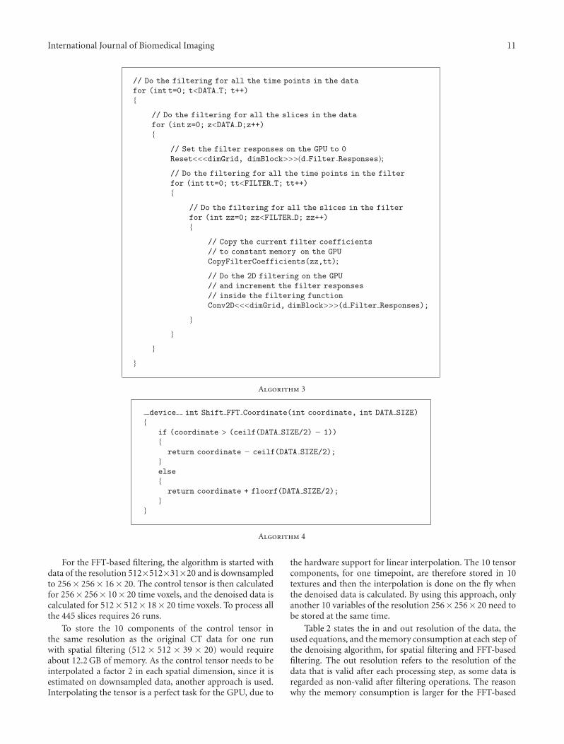
3.3.2. Nonseparable Filtering. The shared memory approachworks rather well for nonseparable 2D filtering but notas well for nonseparable 3D and 4D filtering. The size ofthe shared memory on the Nvidia GTX 580 is 48 KB foreach multiprocessor, and it is thereby only possible to, forexample, fit 11 × 11 × 11 × 9 float values into it. If the 4Dfilter is of size 9×9×9×9, only 3×3×3×1 = 27 valid filterresponses can be generated for each multiprocessor. A betterapproach for nonseparable filtering in 4D is to instead use anoptimized 2D filtering kernel, and then accumulate the filterresponses by summing over the other dimensions by callingthe 2D filtering function for each slice and each time pointof the filter. The approach is described with the pseudocodegiven in Algorithm 3.

Our nonseparable 2D convolver first reads 64 × 64pixels into the shared memory, then calculates the validfilter responses for all the 14 monomial filters or all the 11reconstruction filters at the same time, and finally writesthe results to global memory. Two versions of the convolverwere implemented, one that maximally supports 7× 7 filtersand one that maximally supports 11 × 11 filters. The firstcalculates 58 × 58 valid filter responses, and the secondcalculates 54 × 54 valid filter responses. As 64 × 64 floatvalues only require 16 KB of memory, three thread blocks canrun at the same time on each multiprocessor. This results in58 × 58 × 3 = 10092 and 54 × 54 × 3 = 8748 valid filterresponses per multiprocessor. For optimal performance, the2D filtering loop was completely unrolled by generating thecode with a Matlab script.

The 14 monomial filters are of size 7 × 7 × 7 × 7, thiswould require 135 KB of memory to be stored as floats, butthe constant memory is only 64 KB. For this reason, 7×7 filtercoefficients are stored at a time and are then updated for eachtime point and for each slice. It would be possible to store7× 7× 7 filter coefficients at a time, but by only storing 7× 7coefficients, the size of the filters (2.75 KB) is small enough toalways be in the cache of the constant memory (8 KB). Thesame approach is used for the 11 reconstruction filters of size11× 11× 11× 11.

3.4. FFT-Based Filtering. While the CUFFT library by Nvidiasupports 1D, 2D, and 3D FFTs, there is no direct supportfor 4D FFTs. As the FFT is cartesian separable, it is howeverpossible to do a 4D FFT by applying four consecutive 1DFFTs. The CUFFT library supports launching a batch of 1DFFTs, such that many 1D FFT’s can run in parallel. Thebatch of 1D FFTs are applied along the first dimension inwhich the data is stored (e.g., along x if the data is stored


// Code that is executed before the kernel is launched

int threadsInX = 32;

int threadsInY = 16;

int blocksInX = DATA W/threadsInX;

int blocksInX = DATA H/threadsInY;

dimGrid = dim3(blocksInX, blocksInY);

dimBlock = dim3(threadsInX, threadsInY, 1);

// Code that is executed inside the kernel

int x = blockIdx.x ∗ blockDim.x + threadIdx.x;

int y = blockIdx.y ∗ blockDim.y + threadIx.yd;

Algorithm 1

// Code that is executed before the kernel is launched

int threadsInX = 32;

int threadsInY = 16;

int threadsInZ = 1;

int blocksInX = (DATA W+threadsInX-1)/threadsInX;

int blocksInY = (DATA H+threadsInY-1)/threadsInY;

int blocksInZ = (DATA D+threadsInZ-1)/threadsInZ;

dim3 dimGrid = dim3(blocksInX, blocksInY∗blocksInZ);dim3 dimBlock = dim3(threadsInX, threadsInY, threadsInZ);

// Code that is executed inside the kernel

int blockIdxz = float2uint rd(blockIdx.y ∗ invBlocksInY);

int blockIdxy = blockIdx.y − blockIdxz ∗ blocksInY;

int x = blockIdx.x ∗ blockDim.x + threadIdx.x;

int y = blockIdxy ∗ blockDim.y + threadIdx.y;

int z = blockIdxz ∗ blockDim.z + threadIdx.z;

Algorithm 2

as (x, y, z, t)). Between each 1D FFT, it is thereby necessaryto change the order of the data (e.g., from (x, y, z, t) to(y, z, t, x)). The drawback with this approach is that the timeit takes to change order of the data can be longer than toactually perform the 1D FFT. The most recent version of theCUFFT library supports launching a batch of 2D FFT’s. Byapplying two consecutive 2D FFT’s, it is sufficient to changethe order of the data once, instead of three times.

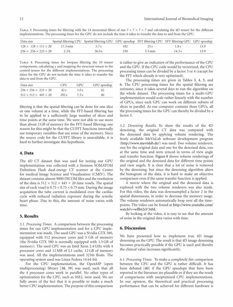
A forward 4D FFT is first applied to the volumes. Afilter is padded with zeros to the same resolution as the dataand is then transformed to the frequency domain. To dothe filtering, a complex-valued multiplication between thedata and the filter is applied and then an inverse 4D FFT isapplied to the filter response. After the inverse transform, aFFT shift is necessary; there is however no such functionalityin the CUFFT library. When the tensor components and thedenoised data are calculated, each of the four coordinates isshifted by using a help function, see Algorithm 4.

As the monomial filters only have a real part or animaginary part in the spatial domain, some additional timeis saved by putting one monomial filter in the real part andanother monomial filter in the imaginary part before the 4DFFT is applied to the zero-padded filter. When the complexmultiplication is performed in the frequency domain, two

filters are thus applied at the same time. After the inverse 4DFFT, the first filter response is extracted as the real part andsecond filter response is extracted as the imaginary part. Thesame trick is used for the 10 highpass reconstruction filters.

3.5. Memory Considerations. The main problem of imple-menting the 4D denoising algorithm on the GPU is thelimited size of the global memory (3 GB in our case). This ismade even more difficult by the fact that the GPU driver canuse as much as 100–200 MB of the global memory. Storingall the CT data on the GPU at the same time is not possible, asingle CT volume of the resolution 512× 512× 445 requiresabout 467 MB of memory if 32 bit floats are used. Storing thefilter responses is even more problematic. To give an example,to store all the 11 reconstruction filter responses as floats fora dataset of the size 512 × 512 × 445 × 20 would requireabout 103 GB of memory. The denoising is therefore donefor a number of slices (e.g., 16 or 32) at a time.

For the spatial filtering, the algorithm is started with dataof the resolution 512 × 512 × 51 × 20 and is downsampledto 256 × 256 × 26 × 20. The control tensor is calculated for256 × 256 × 20 × 20 time voxels, and the denoised data iscalculated for 512× 512× 39× 20 time voxels. To process allthe 445 slices requires 12 runs.


// Do the filtering for all the time points in the data

for (int t=0; t<DATA T; t++)

{// Do the filtering for all the slices in the data

for (int z=0; z<DATA D;z++)

{// Set the filter responses on the GPU to 0

Reset<<<dimGrid, dimBlock>>>(d Filter Responses);

// Do the filtering for all the time points in the filter

for (int tt=0; tt<FILTER T; tt++)

{// Do the filtering for all the slices in the filter

for (int zz=0; zz<FILTER D; zz++)

{// Copy the current filter coefficients

// to constant memory on the GPU

CopyFilterCoefficients(zz,tt);

// Do the 2D filtering on the GPU

// and increment the filter responses

// inside the filtering function

Conv2D<<<dimGrid, dimBlock>>>(d Filter Responses);

}}

}}

Algorithm 3

device int Shift FFT Coordinate(int coordinate, int DATA SIZE)

{if (coordinate > (ceilf(DATA SIZE/2) − 1))

{return coordinate − ceilf(DATA SIZE/2);

}else

{return coordinate + floorf(DATA SIZE/2);

}}

Algorithm 4

For the FFT-based filtering, the algorithm is started withdata of the resolution 512×512×31×20 and is downsampledto 256× 256× 16× 20. The control tensor is then calculatedfor 256× 256× 10× 20 time voxels, and the denoised data iscalculated for 512× 512× 18× 20 time voxels. To process allthe 445 slices requires 26 runs.

To store the 10 components of the control tensor inthe same resolution as the original CT data for one runwith spatial filtering (512 × 512 × 39 × 20) would requireabout 12.2 GB of memory. As the control tensor needs to beinterpolated a factor 2 in each spatial dimension, since it isestimated on downsampled data, another approach is used.Interpolating the tensor is a perfect task for the GPU, due to

the hardware support for linear interpolation. The 10 tensorcomponents, for one timepoint, are therefore stored in 10textures and then the interpolation is done on the fly whenthe denoised data is calculated. By using this approach, onlyanother 10 variables of the resolution 256× 256× 20 need tobe stored at the same time.

Table 2 states the in and out resolution of the data, theused equations, and the memory consumption at each step ofthe denoising algorithm, for spatial filtering and FFT-basedfiltering. The out resolution refers to the resolution of thedata that is valid after each processing step, as some data isregarded as non-valid after filtering operations. The reasonwhy the memory consumption is larger for the FFT-based


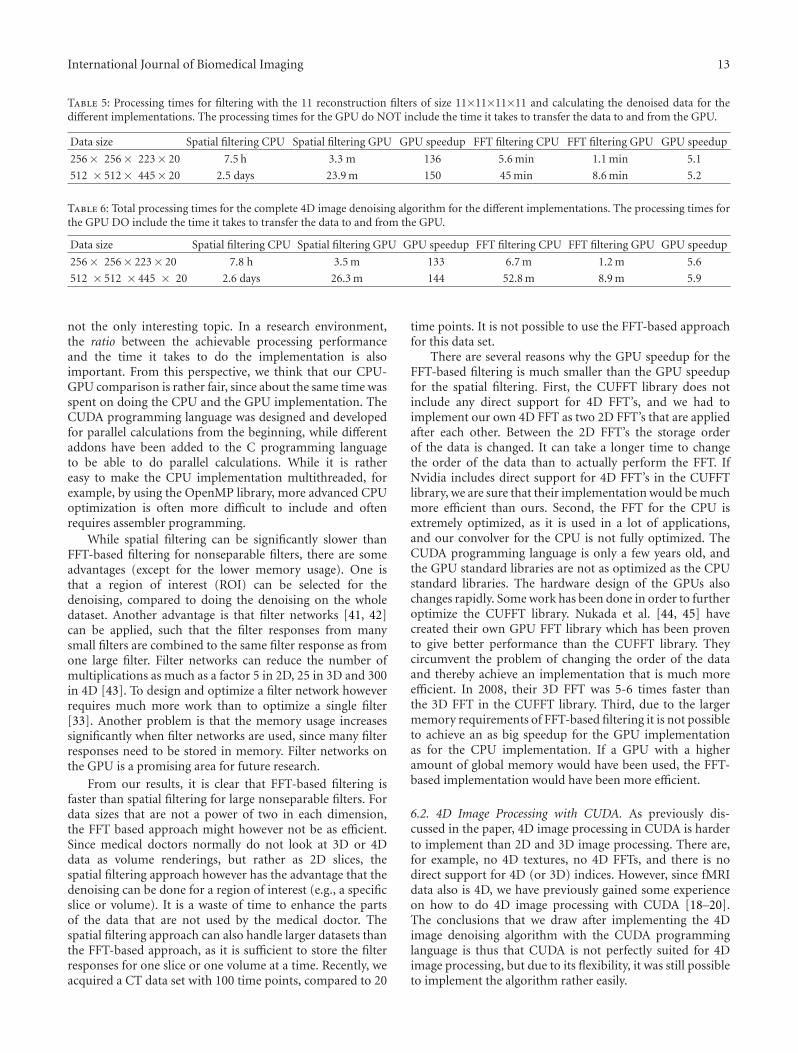
Table 3: Processing times for filtering with the 14 monomial filters of size 7 × 7 × 7 × 7 and calculating the 4D tensor for the differentimplementations. The processing times for the GPU do not include the time it takes to transfer the data to and from the GPU.

Data size Spatial filtering CPU Spatial filtering GPU GPU speedup FFT filtering CPU FFT filtering GPU GPU speedup

128× 128× 111× 20 17.3 min 5.7 s 182 25 s 1.8 s 13.9

256× 256× 223× 20 2.3 h 36.0 s 230 3.3 min 14.3 s 13.9

Table 4: Processing times for lowpass filtering the 10 tensorcomponents, calculating γ and mapping the structure tensor to thecontrol tensor for the different implementations. The processingtimes for the GPU do not include the time it takes to transfer thedata to and from the GPU.

Data size CPU GPU GPU speedup

256× 256× 223× 20 42 s 1.0 s 42

512× 512× 445× 20 292 s 7.3 s 40

filtering is that the spatial filtering can be done for one sliceor one volume at a time, while the FFT-based filtering hasto be applied to a sufficiently large number of slices andtime points at the same time. We were not able to use morethan about 2 GB of memory for the FFT-based filtering; onereason for this might be that the CUFFT functions internallyuse temporary variables that use some of the memory. Sincethe source code for the CUFFT library is unavailable, it ishard to further investigate this hypothesis.

4. Data

The 4D CT dataset that was used for testing our GPUimplementation was collected with a Siemens SOMATOMDefinition Flash dual-energy CT scanner at the Centerfor medical Image Science and Visualization (CMIV). Thedataset contains almost 9000 DICOM files and the resolutionof the data is 512 × 512 × 445 × 20 time voxels. The spatialsize of each voxel is 0.75× 0.75× 0.75 mm. During the imageacquisition the tube current is modulated over the cardiaccycle with reduced radiation exposure during the systolicheart phase. Due to this, the amount of noise varies withtime.

5. Results

5.1. Processing Times. A comparison between the processingtimes for our GPU implementation and for a CPU imple-mentation was made. The used GPU was a Nvidia GTX 580,equipped with 512 processor cores and 3 GB of memory(the Nvidia GTX 580 is normally equipped with 1.5 GB ofmemory). The used CPU was an Intel Xeon 2.4 GHz with 4processor cores and 12 MB of L3 cache, 12 GB of memorywas used. All the implementations used 32 bit floats. Theoperating system used was Linux Fedora 14 64-bit.

For the CPU implementation, the OpenMP (openmultiprocessing) library [38, 39] was used, such that allthe 4 processor cores work in parallel. No other types ofoptimization for the CPU, such as SSE2, were used. We arefully aware of the fact that it is possible to make a muchbetter CPU implementation. The purpose of this comparison

is rather to give an indication of the performance of the CPUand the GPU. If the CPU code would be vectorized, the CPUprocessing times can be divided by a factor 3 or 4 (except forthe FFT which already is very optimized).

The processing times are given in Tables 3, 4, 5, and6. The CPU processing times for the spatial filtering areestimates, since it takes several days to run the algorithm onthe whole dataset. The processing times for a multi-GPUimplementation would scale rather linearly with the numberof GPUs, since each GPU can work on different subsets ofslices in parallel. As our computer contains three GPUs, allthe processing times for the GPU can thereby be divided by afactor 3.

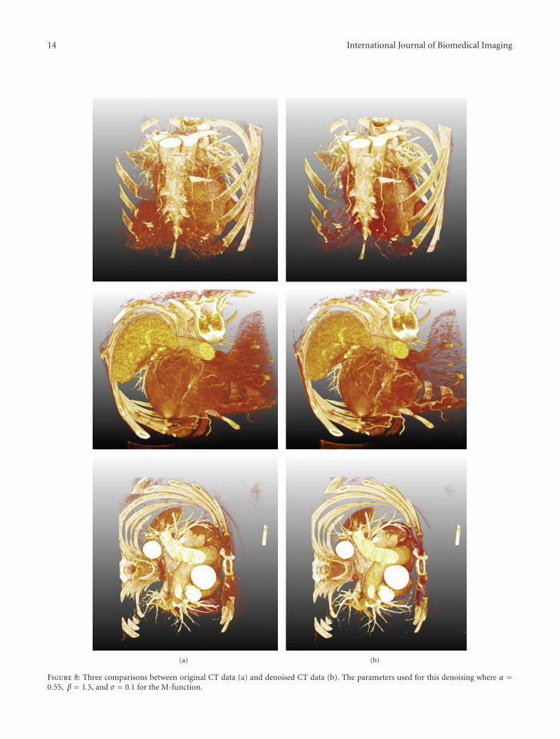
5.2. Denoising Results. To show the results of the 4Ddenoising, the original CT data was compared withthe denoised data by applying volume rendering. Thefreely available MeVisLab software development program(http://www.mevislab.de/) was used. Two volume renderers,one for the original data and one for the denoised data, runat the same time and were synced in terms of view angleand transfer function. Figure 8 shows volume renderings ofthe original and the denoised data for different time pointsand view angels. It is clear that a lot of noise is removedby the denoising, but since the denoising algorithm altersthe histogram of the data, it is hard to make an objectivecomparison even if the same transfer function is applied.

A movie where the original and the denoised data isexplored with the two volume renderers was also made.For this video, the data was downsampled a factor 2 in thespatial dimensions, in order to decrease the memory usage.The volume renderers automatically loop over all the time-points. The video can be found at http://www.youtube.com/watch?v=wflbt2sV34M.

By looking at the video, it is easy to see that the amountof noise in the original data varies with time.

6. Discussion

We have presented how to implement true 4D imagedenoising on the GPU. The result is that 4D image denoisingbecomes practically possible if the GPU is used and therebythe clinical value increases significantly.

6.1. Processing Times. To make a completely fair comparisonbetween the CPU and the GPU is rather difficult. It hasbeen debated [40] if the GPU speedups that have beenreported in the literature are plausible or if they are the resultof comparisons with unoptimized CPU implementations.In our opinion, the theoretical and practical processingperformance that can be achieved for different hardware is


Table 5: Processing times for filtering with the 11 reconstruction filters of size 11×11×11×11 and calculating the denoised data for thedifferent implementations. The processing times for the GPU do NOT include the time it takes to transfer the data to and from the GPU.


256× 256× 223× 20 7.5 h 3.3 m 136 5.6 min 1.1 min 5.1

512 × 512× 445× 20 2.5 days 23.9 m 150 45 min 8.6 min 5.2

Table 6: Total processing times for the complete 4D image denoising algorithm for the different implementations. The processing times forthe GPU DO include the time it takes to transfer the data to and from the GPU.


256× 256× 223× 20 7.8 h 3.5 m 133 6.7 m 1.2 m 5.6

512 × 512 × 445 × 20 2.6 days 26.3 m 144 52.8 m 8.9 m 5.9

not the only interesting topic. In a research environment,the ratio between the achievable processing performanceand the time it takes to do the implementation is alsoimportant. From this perspective, we think that our CPU-GPU comparison is rather fair, since about the same time wasspent on doing the CPU and the GPU implementation. TheCUDA programming language was designed and developedfor parallel calculations from the beginning, while differentaddons have been added to the C programming languageto be able to do parallel calculations. While it is rathereasy to make the CPU implementation multithreaded, forexample, by using the OpenMP library, more advanced CPUoptimization is often more difficult to include and oftenrequires assembler programming.

While spatial filtering can be significantly slower thanFFT-based filtering for nonseparable filters, there are someadvantages (except for the lower memory usage). One isthat a region of interest (ROI) can be selected for thedenoising, compared to doing the denoising on the wholedataset. Another advantage is that filter networks [41, 42]can be applied, such that the filter responses from manysmall filters are combined to the same filter response as fromone large filter. Filter networks can reduce the number ofmultiplications as much as a factor 5 in 2D, 25 in 3D and 300in 4D [43]. To design and optimize a filter network howeverrequires much more work than to optimize a single filter[33]. Another problem is that the memory usage increasessignificantly when filter networks are used, since many filterresponses need to be stored in memory. Filter networks onthe GPU is a promising area for future research.

From our results, it is clear that FFT-based filtering isfaster than spatial filtering for large nonseparable filters. Fordata sizes that are not a power of two in each dimension,the FFT based approach might however not be as efficient.Since medical doctors normally do not look at 3D or 4Ddata as volume renderings, but rather as 2D slices, thespatial filtering approach however has the advantage that thedenoising can be done for a region of interest (e.g., a specificslice or volume). It is a waste of time to enhance the partsof the data that are not used by the medical doctor. Thespatial filtering approach can also handle larger datasets thanthe FFT-based approach, as it is sufficient to store the filterresponses for one slice or one volume at a time. Recently, weacquired a CT data set with 100 time points, compared to 20

time points. It is not possible to use the FFT-based approachfor this data set.

There are several reasons why the GPU speedup for theFFT-based filtering is much smaller than the GPU speedupfor the spatial filtering. First, the CUFFT library does notinclude any direct support for 4D FFT’s, and we had toimplement our own 4D FFT as two 2D FFT’s that are appliedafter each other. Between the 2D FFT’s the storage orderof the data is changed. It can take a longer time to changethe order of the data than to actually perform the FFT. IfNvidia includes direct support for 4D FFT’s in the CUFFTlibrary, we are sure that their implementation would be muchmore efficient than ours. Second, the FFT for the CPU isextremely optimized, as it is used in a lot of applications,and our convolver for the CPU is not fully optimized. TheCUDA programming language is only a few years old, andthe GPU standard libraries are not as optimized as the CPUstandard libraries. The hardware design of the GPUs alsochanges rapidly. Some work has been done in order to furtheroptimize the CUFFT library. Nukada et al. [44, 45] havecreated their own GPU FFT library which has been provento give better performance than the CUFFT library. Theycircumvent the problem of changing the order of the dataand thereby achieve an implementation that is much moreefficient. In 2008, their 3D FFT was 5-6 times faster thanthe 3D FFT in the CUFFT library. Third, due to the largermemory requirements of FFT-based filtering it is not possibleto achieve an as big speedup for the GPU implementationas for the CPU implementation. If a GPU with a higheramount of global memory would have been used, the FFT-based implementation would have been more efficient.

6.2. 4D Image Processing with CUDA. As previously dis-cussed in the paper, 4D image processing in CUDA is harderto implement than 2D and 3D image processing. There are,for example, no 4D textures, no 4D FFTs, and there is nodirect support for 4D (or 3D) indices. However, since fMRIdata also is 4D, we have previously gained some experienceon how to do 4D image processing with CUDA [18–20].The conclusions that we draw after implementing the 4Dimage denoising algorithm with the CUDA programminglanguage is thus that CUDA is not perfectly suited for 4Dimage processing, but due to its flexibility, it was still possibleto implement the algorithm rather easily.


(a) (b)

Figure 8: Three comparisons between original CT data (a) and denoised CT data (b). The parameters used for this denoising where α =0.55, β = 1.5, and σ = 0.1 for the M-function.


6.3. True 5D Image Denoising. It might seem impossible tohave medical image data with more than 4 dimensions, butsome work has been done on how to collect 5D data [46].The five dimensions are the three spatial dimensions and twotime dimensions, one for the breathing rhythm and one forthe heart rhythm. One major advantage with 5D data is thatthe patient can breathe normally during the data acquisition,while the patient has to hold its breath during collection of4D data. With 5D data, it is possible to, for example, fixatethe heart and only see the lungs moving, or fixate the lungsto only see the heart beating. If the presented algorithmwould be extended to 5D, it would be necessary to use atotal of 20 monomial filters and 16 reconstruction filters.For a 5D dataset of the size 512 × 512 × 445 × 20 × 20,the required number of multiplications for spatial filteringwith the reconstruction filters would increase from 375 000billion for 4D to about 119 million billion (1.19 · 1017) for5D. The size of the reconstruction filter responses wouldincrease from 103 GB for 4D to 2986 GB for 5D. This is stillonly one dataset for one patient, and we expect that both thespatial and the temporal resolution of all medical imagingmodalities will increase even further in the future. Except forthe 5 outer dimensions, it is also possible to collect data withmore than one inner dimension. This is, for example, the caseif the blood flow of the heart is to be studied. For flow data,a three-dimensional vector needs to be stored in each timevoxel, instead of a single intensity value.

7. Conclusions

To conclude, by using the GPU, true 4D image denoisingbecomes practically feasible. Our implementation can ofcourse be applied to other modalities as well, such as ultra-sound and MRI, and not only to CT data. The short process-ing time also makes it practically possible to further improvethe denoising algorithm and to tune the parameters that areused.

The elapsed time between the development of practicallyfeasible 2D [2] and 3D [4] image denoising techniques wasabout 10 years, from 3D to 4D the elapsed time was about 20years. Due to the rapid development of GPUs, it is hopefullynot necessary to wait another 10–20 years for 5D imagedenoising.

Acknowledgments

This work was supported by the Linnaeus Center CADICSand research Grant no. 2008-3813, funded by the Swedishresearch council. The CT data was collected at the Centerfor Medical Image Science and Visualization (CMIV). Theauthors would like to thank the NovaMedTech project atLinkoping University for financial support of the GPUhardware, Johan Wiklund for support with the CUDAinstallations, and Chunliang Wang for setting the transferfunctions for the volume rendering.

References

[1] J.-S. Lee, “Digital image enhancement and noise filtering byuse of local statistics,” IEEE Transactions on Pattern Analysisand Machine Intelligence, vol. 2, no. 2, pp. 165–168, 1980.

[2] H. E. Knutsson, R. Wilson, and G. H. Granlund, “Anisotropicnon-stationary image estimation and its applications—part I:restoration of noisy images,” IEEE Transactions on Communi-cations, vol. 31, no. 3, pp. 388–397, 1983.

[3] P. Perona and J. Malik, “Scale-space and edge detection usinganisotropic diffusion,” IEEE Transactions on Pattern Analysisand Machine Intelligence, vol. 12, no. 7, pp. 629–639, 1990.

[4] H. Knutsson, L. Haglund, H. Barman, and G. Granlund,“A framework for anisotropic adaptive filtering and analysisof image sequences and volumes,” in Proceedings of theIEEE International Conference on Acoustics, Speech and SignalProcessing, (ICASSP), pp. 469–472, 1992.

[5] G. Granlund and H. Knutsson, Signal Processing for ComputerVision, Kluwer Academic, Boston, Mass, USA, 1995.

[6] C.-F. Westin, L. Wigstrom, T. Loock, L. Sjoqvist, R. Kikinis,and H. Knutsson, “Three-dimensional adaptive filtering inmagnetic resonance angiography,” Journal of Magnetic Reso-nance Imaging, vol. 14, pp. 63–71, 2001.

[7] J. Montagnat, M. Sermesant, H. Delingette, G. Malandain, andN. Ayache, “Anisotropic filtering for model-based segmen-tation of 4D cylindrical echocardiographic images,” PatternRecognition Letters, vol. 24, no. 4-5, pp. 815–825, 2003.

[8] H. Jahanian, A. Yazdan-Shahmorad, and H. Soltanian-Zadeh,“4D wavelet noise suppression of MR diffusion tensor data,” inProceedings of the IEEE International Conference on Acoustics,Speech and Signal Processing, (ICASSP), pp. 509–512, April2008.

[9] K. Pauwels and M. M. Van Hulle, “Realtime phase-basedoptical flow on the GPU,” in Proceedings of the IEEE ComputerSociety Conference on Computer Vision and Pattern RecognitionWorkshops, (CVPR), pp. 1–8, June 2008.

[10] P. Muyan-Ozcelik, J. D. Owens, J. Xia, and S. S. Samant, “Fastdeformable registration on the GPU: a CUDA implementationof demons,” in Proceedings of the International Conference onComputational Sciences and its Applications, (ICCSA), pp. 223–233, July 2008.

[11] P. Bui and J. Brockman, “Performance analysis of acceleratedimage registration using GPGPU,” in Proceedings of the 2ndWorkshop on General Purpose Processing on Graphics ProcessingUnits, (GPGPU-2), pp. 38–45, March 2009.

[12] A. Eklund, M. Andersson, and H. Knutsson, “Phase basedvolume registration using CUDA,” in Proceedings of theIEEE International Conference on Acoustics, Speech, and SignalProcessing, (ICASSP), pp. 658–661, March 2010.

[13] R. Shams, P. Sadeghi, R. Kennedy, and R. Hartley, “A survey ofmedical image registration on multicore and the GPU,” IEEESignal Processing Magazine, vol. 27, no. 2, Article ID 5438962,pp. 50–60, 2010.

[14] A. E. Lefohn, J. E. Cates, and R. T. Whitaker, “Interactive,GPU-based level sets for 3D segmentation,” Lecture Notes inComputer Science, vol. 2878, pp. 564–572, 2003.

[15] V. Vineet and P. J. Narayanan, “CUDA cuts: fast graphcuts on the GPU,” in Proceedings of the IEEE ComputerSociety Conference on Computer Vision and Pattern RecognitionWorkshops, (CVPR), pp. 1–8, June 2008.

[16] A. Abramov, T. Kulvicius, F. Worgotter, and B. Dellen, “Real-time image segmentation on a GPU,” in Proceedings of Facingthe Multicore-Challenge, vol. 6310 of Lecture Notes in ComputerScience, pp. 131–142, Springer, 2011.


[17] D. Gembris, M. Neeb, M. Gipp, A. Kugel, and R. Manner,“Correlation analysis on GPU systems using NVIDIA’sCUDA,” Journal of Real-Time Image Processing, pp. 1–6, 2010.

[18] A. Eklund, O. Friman, M. Andersson, and H. Knutsson, “AGPU accelerated interactive interface for exploratory func-tional connectivity analysis of fMRI data,” in Proceedings of theIEEE International Conference on Image Processing, (ICIP), pp.1621–1624, 2011.

[19] A. Eklund, M. Andersson, and H. Knutsson, “fMRI analysison the GPU—possibilities and challenges,” Computer Methodsand Programs in Biomedicine. In press.

[20] A. Eklund, M. Andersson, and H. Knutsson, “Fast randompermutation tests enable objective evaluation of methodsfor single subject fMRI analysis,” International Journal ofBiomedical Imaging, vol. 2011, Article ID 627947, 2011.

[21] M. Rumpf and R. Strzodka, “Nonlinear diffusion in graphicshardware,” in Proceedings of the EG/IEEE TCVG Symposium onVisualization, pp. 75–84, 2001.

[22] M. Howison, “Comparing GPU implementations of bilateraland anisotropic diffusion filters for 3D biomedical datasets,”Tech. Rep. LBNL-3425E, Lawrence Berkeley National Labora-tory, Berkeley, Calif, USA.

[23] Y. Su and Z. Xu, “Parallel implementation of wavelet-based image denoising on programmable PC-grade graphicshardware,” Signal Processing, vol. 90, no. 8, pp. 2396–2411,2010.

[24] Q. Zhang, R. Eagleson, and T. M. Peters, “GPU-based imagemanipulation and enhancement techniques for dynamic vol-umetric medical image visualization,” in Proceedings of the 4thIEEE International Symposium on Biomedical Imaging: FromNano to Macro, (ISBI), pp. 1168–1171, April 2007.

[25] J. Chen, S. Paris, and F. Durand, “Real-time edge-awareimage processing with the bilateral grid, ACM transactionson graphics,” in Proceedings of the Special Interest Group onComputer Graphics and Interactive Techniques Conference, no.103, p. 9, 2007.

[26] C. Tomasi and R. Manduchi, “Bilateral filtering for gray andcolor images,” in Proceedings of the IEEE 6th InternationalConference on Computer Vision, pp. 839–846, January 1998.

[27] F. Fontes, G. Barroso, P. Coupe, and P. Hellier, “Real timeultrasound image denoising,” Journal of Real-Time ImageProcessing, vol. 6, pp. 15–22, 2010.

[28] B. Goossens, H. Luong, J. Aelterman, A. Pizurica, and W.Philips, “A GPU-accelerated real-time NLMeans algorithm fordenoising color video sequences,” in Proceedings of the 12thInternational Conference on Advanced Concepts for IntelligentVision Systems, (ACIVS), vol. 6475 of Lecture Notes in Com-puter Science, pp. 46–57, Springer, 2010.

[29] A. Buades, B. Coll, and J. M. Morel, “A non-local algorithm forimage denoising,” in Proceedings of the IEEE Computer SocietyConference on Computer Vision and Pattern Recognition,(CVPR), pp. 60–65, June 2005.

[30] H. Knutsson, “Representing local structure using tensors,” inProceedings of the Scandinavian Conference on Image Analysis,(SCIA), pp. 244–251, 1989.

[31] F. Forsberg, V. Berghella, D. A. Merton, K. Rychlak, J. Meiers,and B. B. Goldberg, “Comparing image processing techniquesfor improved 3-dimensional ultrasound imaging,” Journal ofUltrasound in Medicine, vol. 29, no. 4, pp. 615–619, 2010.

[32] H. Knutsson, C.-F. Westin, and M. Andersson, “Representinglocal structure using tensors II,” in Proceedings of the Scandina-vian Conference on Image Analysis, (SCIA), vol. 6688 of LectureNotes in Computer Science, pp. 545–556, Springer, 2011.

[33] H. Knutsson, M. Andersson, and J. Wiklund, “Advanced filterdesign,” in Proceedings of the Scandinavian Conference onImage Analysis, (SCIA), pp. 185–193, 1999.

[34] H. Knutsson and C. F. Westin, “Normalized and differen-tial convolution: methods for interpolation and filtering ofincomplete and uncertain data,” in Proceedings of the IEEEComputer Society Conference on Computer Vision and PatternRecognition, (CVPR), pp. 515–523, June 1993.

[35] Nvidia, CUDA Programming Guide, Version 4.0., 2011.[36] D. Kirk and W. Hwu, Programming Massively Parallel Pro-

cessors, A Handson Approach, Morgan Kaufmann, Waltham,Mass, USA, 2010.

[37] The Khronos Group & OpenCL, 2010, http://www.khronos.org/opencl/.

[38] The OpenMP API specification for parallel programming,2011, http://www.openmp.org/.

[39] B. Chapman, G. Jost, and R. van der Pas, Using OpenMP,Portable Shared Memory Parallel Programming, MIT Press,Cambridge, Mass, USA, 2007.

[40] V. W. Lee, C. Kim, J. Chhugani et al., “Debunking the 100XGPU vs. CPU Myth: an evaluation of throughput computingon CPU and GPU,” in Proceedings of the 37th InternationalSymposium on Computer Architecture, (ISCA), pp. 451–460,June 2010.

[41] M. Andersson, J. Wiklund, and H. Knutsson, “Filter net-works,” in Proceedings of the Signal and Image Processing, (SIP),pp. 213–217, 1999.

[42] B. Svensson, M. Andersson, and H. Knutsson, “Filter networksfor efficient estimation of local 3-D structure,” in Proceedingsof the IEEE International Conference on Image Processing,(ICIP), pp. 573–576, September 2005.

[43] M. Andersson, J. Wiklund, and H. Knutsson, “Sequential filtertrees for efficient 2D, 3D and 4D orientation estimation,” Tech.Rep. LiTH-ISY-R-2070, Department of Electrical Engineering,Linkoping University, Linkoping, Sweden, 1998.

[44] A. Nukada, Y. Ogata, T. Endo, and S. Matsuoka, “Bandwidthintensive 3-D FFT kernel for GPUs using CUDA,” in Pro-ceedings of the International Conference for High PerformanceComputing, Networking, Storage and Analysis, (SC), pp. 1–11,November 2008.

[45] A. Nukada and S. Matsuoka, “Auto-tuning 3-D FFT library forCUDA GPUs,” in Proceedings of the International Conferenceon High Performance Computing Networking, Storage andAnalysis, (SC), pp. 1–10, November 2009.

[46] A. Sigfridsson, J. P. E. Kvitting, H. Knutsson, and L. Wigstrom,“Five-dimensional MRI incorporating simultaneous resolu-tion of cardiac and respiratory phases for volumetric imaging,”Journal of Magnetic Resonance Imaging, vol. 25, no. 1, pp. 113–121, 2007.

true 4d image denoising on the gpu - diva...

Documents