tropospheric chemistry in the integrated forecasting system of
TRANSCRIPT
Geosci. Model Dev., 8, 975–1003, 2015
www.geosci-model-dev.net/8/975/2015/
doi:10.5194/gmd-8-975-2015
© Author(s) 2015. CC Attribution 3.0 License.
Tropospheric chemistry in the Integrated Forecasting
System of ECMWF
J. Flemming1, V. Huijnen2, J. Arteta3, P. Bechtold1, A. Beljaars1, A.-M. Blechschmidt4, M. Diamantakis1,
R. J. Engelen1, A. Gaudel5, A. Inness1, L. Jones1, B. Josse3, E. Katragkou6, V. Marecal3, V.-H. Peuch1, A. Richter4,
M. G. Schultz7, O. Stein7, and A. Tsikerdekis6
1European Centre for Medium-Range Weather Forecasts, Reading, UK2Royal Netherlands Meteorological Institute, De Belt, the Netherlands3Météo-France, Toulouse, France4Universität Bremen, Bremen, Germany5CNRS, Laboratoire d’Aérologie, UMR 5560, Toulouse, France6Department of Meteorology and Climatology, School of Geology, Aristotle University of Thessaloniki, Thessaloniki, Greece7Institute for Energy and Climate Research, Forschungszentrum Jülich, Jülich, Germany
Correspondence to: J. Flemming ([email protected])
Received: 10 September 2014 – Published in Geosci. Model Dev. Discuss.: 18 November 2014
Revised: 3 March 2015 – Accepted: 12 March 2015 – Published: 7 April 2015
Abstract. A representation of atmospheric chemistry has
been included in the Integrated Forecasting System (IFS)
of the European Centre for Medium-Range Weather Fore-
casts (ECMWF). The new chemistry modules complement
the aerosol modules of the IFS for atmospheric composition,
which is named C-IFS. C-IFS for chemistry supersedes a
coupled system in which chemical transport model (CTM)
Model for OZone and Related chemical Tracers 3 was two-
way coupled to the IFS (IFS-MOZART). This paper contains
a description of the new on-line implementation, an evalua-
tion with observations and a comparison of the performance
of C-IFS with MOZART and with a re-analysis of atmo-
spheric composition produced by IFS-MOZART within the
Monitoring Atmospheric Composition and Climate (MACC)
project. The chemical mechanism of C-IFS is an extended
version of the Carbon Bond 2005 (CB05) chemical mech-
anism as implemented in CTM Transport Model 5 (TM5).
CB05 describes tropospheric chemistry with 54 species and
126 reactions. Wet deposition and lightning nitrogen monox-
ide (NO) emissions are modelled in C-IFS using the de-
tailed input of the IFS physics package. A 1 year simula-
tion by C-IFS, MOZART and the MACC re-analysis is eval-
uated against ozonesondes, carbon monoxide (CO) aircraft
profiles, European surface observations of ozone (O3), CO,
sulfur dioxide (SO2) and nitrogen dioxide (NO2) as well as
satellite retrievals of CO, tropospheric NO2 and formalde-
hyde. Anthropogenic emissions from the MACC/CityZen
(MACCity) inventory and biomass burning emissions from
the Global Fire Assimilation System (GFAS) data set were
used in the simulations by both C-IFS and MOZART. C-
IFS (CB05) showed an improved performance with respect
to MOZART for CO, upper tropospheric O3, and winter-
time SO2, and was of a similar accuracy for other evaluated
species. C-IFS (CB05) is about 10 times more computation-
ally efficient than IFS-MOZART.
1 Introduction
Monitoring and forecasting of global atmospheric compo-
sition are key objectives of the atmosphere service of the
European Copernicus programme. The Copernicus Atmo-
sphere Monitoring Service (CAMS) is based on combining
satellite observations of atmospheric composition with state-
of-the-art atmospheric modelling (Flemming et al., 2013;
Hollingsworth et al., 2008). For that purpose, the Inte-
grated Forecasting System (IFS) of the European Centre for
Medium-Range Weather Forecasts (ECMWF) was extended
for forecast and assimilation of atmospheric composition.
Modules for aerosols (Morcrette et al., 2009; Benedetti et
Published by Copernicus Publications on behalf of the European Geosciences Union.

976 J. Flemming et al.: Tropospheric chemistry in the Integrated Forecasting System of ECMWF
al., 2009) and greenhouse gases (Engelen et al., 2009) were
integrated on-line in the IFS. Because of the complexity of
the chemical mechanisms for reactive gases, modules for at-
mospheric chemistry were not initially included in the IFS.
Instead, a coupled system (Flemming et al., 2009a) was de-
veloped, which couples the IFS to chemical transport model
(CTM) Model for OZone and Related chemical Tracers 3
(MOZART, Kinnison et al., 2007) or Transport Model 5
(TM5, Huijnen et al., 2010) by means of the Ocean Atmo-
sphere Sea Ice Soil (OASIS4) coupler software (Redler et al.,
2010). Van Noije et al. (2014) coupled TM5 to IFS for cli-
mate applications in a similar approach. The coupled system
made it possible to assimilate satellite retrievals of reactive
gases with the assimilation algorithm of the IFS, which is
also used for the assimilation of meteorological observations
as well as for aerosol and greenhouse gases.
Coupled system IFS-MOZART has been successfully
used for a re-analysis of atmospheric composition (Inness
et al., 2013), pre-operational atmospheric composition fore-
casts (Stein et al., 2012), and forecast and assimilation of the
stratospheric ozone (O3) (Flemming et al., 2011; Lefever et
al., 2014), tropospheric carbon monoxide (CO) (Elguindi et
al., 2010) and O3 (Ordóñez et al., 2010). Coupled system
IFS-TM5 has been used in a case study on a period with
intense biomass burning in Russia in 2010 (Huijnen et al.,
2012). Nevertheless, the coupled approach has limitations
such as the need for interpolation between the IFS and CTM
model grids and the duplicate simulation of transport pro-
cesses. Furthermore, its computational performance is often
not optimal as it can suffer from load imbalances between the
coupled components.
Consequently, modules for atmospheric chemistry and re-
lated physical processes have now been integrated on-line in
the IFS, thereby complementing the on-line integration strat-
egy already pursued for aerosol and greenhouse gases in IFS.
The IFS including modules for atmospheric composition is
named Composition-IFS (C-IFS). C-IFS makes it possible
(i) to use the detailed meteorological simulation of the IFS
for the simulation of the fate of constituents (ii) to use the
IFS data assimilation system to assimilate observations of
atmospheric composition and (iii) to simulate feedback pro-
cesses between atmospheric composition and weather. A fur-
ther advantage of C-IFS is the possibility of model runs at
a high horizontal and vertical resolution because of the high
computational efficiency of C-IFS. C-IFS is the global model
system run in pre-operational mode as part of the Monitoring
Atmospheric Composition and Climate – Interim Implemen-
tation project (MACC II and MACC III) in preparation of
CAMS.
Including chemistry modules in general circulation mod-
els (GCM) to simulate interaction of stratospheric O3 (e.g.
Steil et al., 1998) and aerosols (e.g. Haywood et al., 1997)
in the climate system started in the mid-1990s. Later, more
comprehensive schemes for tropospheric chemistry were in-
cluded in climate GCM such as ECHAM5-HAMMOZ (Poz-
zoli et al., 2008; Rast et al., 2014) and CAM-chem (Lamar-
que et al., 2012) to study short-lived greenhouse gases and
the influence of climate change on air pollution (e.g. Fiore
et al., 2012). In the UK Met Office’s Unified Model (UM),
stratospheric chemistry (Morgenstern et al., 2009) and tropo-
spheric chemistry (O’Connor et al., 2014) can be simulated
together with the GLOMAP mode aerosol scheme (Mann et
al., 2010). Examples of the on-line integration of chemistry
modules in global circulation models with focus on NWP
are GEM-AQ (Kaminski et al., 2008), GEMS-BACH (Mé-
nard et al., 2007) and GU-WRF/Chem (Zhang et al., 2012).
Savage et al. (2013) evaluate the performance of air qual-
ity forecast with the UM on the regional scale. Baklanov et
al. (2014) give a comprehensive overview of on-line coupled
chemistry–meteorological models for regional applications.
C-IFS is intended to run with several chemistry schemes
for both the troposphere and the stratosphere in the future.
Currently, only the tropospheric chemical mechanism CB05
originating from the TM5 CTM (Huijnen et al., 2010) has
been thoroughly tested. For example, C-IFS (CB05) has been
applied to study the HO2 uptake on clouds and aerosols (Hui-
jnen et al., 2014) and pollution in the Arctic (Emmons et
al., 2014). The tropospheric and stratospheric scheme RAC-
MOBUS of the MOCAGE model (Bousserez et al., 2007)
and the MOZART 3 chemical scheme as well as an extension
of the CB05 scheme with the stratospheric chemical mecha-
nism of the BASCOE model (Errera et al., 2008) have been
technically implemented and are being scientifically tested.
Only C-IFS (CB05) is the subject of this paper.
Each chemistry scheme in C-IFS consists of the specific
gas-phase chemical mechanism, multi-phase chemistry, the
calculation of photolysis rates and upper chemical boundary
conditions. Dry and wet deposition, emission injection and
parameterisation of lightning NO emissions as well as trans-
port and diffusion are simulated by the same approach for all
chemistry schemes. Likewise, emissions and dry deposition
input data are kept the same for all configurations.
The purpose of this paper is to document C-IFS and to
present its model performance with respect to observations.
Since C-IFS (CB05) replaced the current operational MACC
model system for reactive gases (IFS-MOZART) both in data
assimilation and forecast mode, the evaluation in this paper is
carried out predominantly with observations that are used for
the routine evaluation of the MACC II system. The model re-
sults are compared (i) with a MOZART stand-alone simula-
tion, which is equivalent to a IFS-MOZART simulation, and
(ii) with the MACC re-analysis (Inness et al., 2013), which is
an application of IFS-MOZART in data assimilation mode.
All model configurations used the same emission data. The
comparison demonstrates that C-IFS is ready to be used op-
erationally.
The paper is structured as follows. Section 2 is a descrip-
tion of the C-IFS, with the focus on the newly implemented
physical parameterisations and the CB05 chemical mecha-
nism. Section 3 contains the evaluation with observations
Geosci. Model Dev., 8, 975–1003, 2015 www.geosci-model-dev.net/8/975/2015/

J. Flemming et al.: Tropospheric chemistry in the Integrated Forecasting System of ECMWF 977
of a 1 year simulation with C-IFS (CB05) and a compari-
son with the results from the MOZART run and the MACC
re-analysis. The paper is concluded with a summary and an
outlook in Sect. 4.
2 Description of C-IFS
2.1 Overview of C-IFS
The IFS consists of a spectral NWP model that applies
the semi-Lagrangian (SL) semi-implicit method to solve
the governing dynamical equations. The simulation of the
hydrological cycle includes prognostic representations of
cloud fraction, cloud liquid water, cloud ice, rain and snow
(Forbes et al., 2011). The simulations presented in this paper
used the IFS release CY40r1. The technical and scientific
documentation of this IFS release can be found at http:
//www.ecmwf.int/en/forecasts/documentation-and-support/
changes-ecmwf-model/cy40r1-summary/cycle-40r1.
Changes in the operational model are documented at https://
software.ecmwf.int/wiki/display/IFS/Operational+changes.
At the start of the time step, the three-dimensional advec-
tion of the tracers mass mixing ratios is simulated by the SL
method as described in Temperton et al. (2001) and Hortal
(2002). Next, the tracers are vertically distributed by the dif-
fusion scheme (Beljaars and Viterbo, 1998) and by convec-
tive mass fluxes (Bechtold et al., 2014). The diffusion scheme
also simulates the injection of emissions and the loss by dry
deposition (see Sect. 2.4.1). The output of the convection
scheme is used to calculate NO production by lightning (see
Sect. 2.4.3). Finally, the sink and source terms due to chemi-
cal conversion (see Sect. 2.5), wet deposition (see Sect. 2.4.2)
and prescribed surface and stratospheric boundary conditions
are calculated (see Sect. 2.5.2).
The chemical species and the related processes are rep-
resented only in grid-point space. The horizontal grid is a
reduced Gaussian grid (Hortal and Simmons, 1991). C-IFS
can be run at varying vertical and horizontal resolutions. The
simulations presented in this paper were carried out at a T255
spectral resolution (i.e. truncation at wave number 255),
which corresponds to a grid box size of about 80 km. The
vertical discretisation uses 60 levels up to the model top at
0.1 hPa (65 km) in a hybrid sigma-pressure coordinate. The
vertical extent of the lowest level is about 17 m; it is 100 m at
about 300 m above ground, 400–600 m in the middle tropo-
sphere and about 800 m at about 10 km in height.
The modus operandi of C-IFS is one of a forecast model
in a NWP framework. The simulations of C-IFS are a se-
quence of daily forecasts over a period of several days. Each
forecast is initialised by the ECMWF’s operational analy-
sis for the meteorological fields and by the 3-D chemistry
fields from the previous forecast (“forecast mode”). Contin-
uous simulations over longer periods are carried out in “re-
laxation mode”. In relaxation mode the meteorological fields
are relaxed to the fields of a meteorological re-analysis, such
as ERA-Interim, during the run (Jung et al., 2008) to ensure
realistic and consistent meteorological fields.
2.2 Transport
The transport by advection, convection and turbulent diffu-
sion of the chemical tracers uses the same algorithms as de-
veloped for the transport of water vapour in the NWP ap-
plications of IFS. The advection is simulated with a three-
dimensional semi-Lagrangian advection scheme, which ap-
plies a quasi-monotonic cubic interpolation of the departure
values. Since the semi-Lagrangian advection does not for-
mally conserve mass, a global mass fixer is applied. The
effect of different global mass fixers is discussed in Dia-
mantakis and Flemming (2014) and Flemming and Huijnen
(2011). A proportional mass fixer was used for the runs pre-
sented in this paper because of the overall best balance be-
tween the results and computational cost.
The vertical turbulent transport in the boundary layer is
represented by a first-order K-diffusion closure. The surface
emissions are injected as lower boundary flux in the diffusion
scheme. The lower boundary flux condition also accounts for
the dry deposition flux based on the projected surface mass
mixing ratio in an implicit way. The vertical transport by
convection is simulated as part of the cumulus convection.
It applies a bulk mass flux scheme which was originally de-
scribed in Tiedtke (1989). The scheme considers deep, shal-
low and mid-level convection. Clouds are represented by
a single pair of entraining/detraining plumes which deter-
mine the updraught and downdraught mass fluxes (http://old.
ecmwf.int/research/ifsdocs/CY40r1/ in Physical Processes,
Chapter 6, pp. 73–90). Highly soluble species such as nitric
acid (HNO3), hydrogen peroxide (H2O2) and aerosol pre-
cursors are assumed to be scavenged in the convective rain
droplets and are therefore excluded from the convective mass
transfer.
The operator splitting between the transport and the sink
and source terms follows the implementation for water
vapour (Beljaars et al., 2004). Advection, diffusion and con-
vection are simulated sequentially. The sink and source pro-
cesses are simulated in parallel using an intermediate update
of the mass mixing ratios with all transport tendencies. At
the end of the time step tendencies from transport and sink
and source terms are added together for the final update the
concentration fields. Resulting negative mass mixing ratios
are corrected at this point by setting the updated mass mix-
ing ratio to a “chemical zero” of 1.0× 10⁻²⁵ kgkg−1. For
the majority of the species the contribution of the negative
fixer was below 0.1 % of the dominating source or sink term.
The contribution was of the order of 1 % for nitrogen species
such as NO, N2O5 as well as up to 3 % for highly soluble
species such HNO3, HO2, NO3_A. Large gradients of NOx
at the terminator in the stratosphere as well as intensive wet
www.geosci-model-dev.net/8/975/2015/ Geosci. Model Dev., 8, 975–1003, 2015

978 J. Flemming et al.: Tropospheric chemistry in the Integrated Forecasting System of ECMWF
Table 1. Annual emissions from anthropogenic, biogenic and natural sources and biomass burning for 2008 in Tg for a C-IFS (CB05) run at
T255 resolution. Anthropogenic NO emissions contain a contribution of 1.8 Tg aircraft emissions and 12.3 Tg (5.7 TgN) lightning emissions
(LiNO) is added in the biomass burning columns.
Species Anthropogenic Biogenic and natural Biomass burning
CO 584 96 328
NO 70+ 1.8 10 9.2+ 12.3 (LiNO)
HCHO 3.4 4.0 4.9
CH3OH 2.2 159 8.5
C2H6 3.4 1.1 2.3
C2H5OH 3.1 0 0
C2H4 7.7 18 4.3
C3H8 4.0 1.3 1.2
C3H6 3.5 7.6 2.5
Parafins (TgC) 31 18 1.7
Olefines (TgC) 2.4 0 0.7
Aldehydes (TgC) 1.1 6.1 2.1
CH3COCH3 1.3 28 2.4
Isoprene 0 523 0
Terpenes 0 97 0
SO2 98 9 2.2
DMS 0 38 0.2
NH3 40 11 6.2
deposition were the reasons for the increased occurrence of
projected negative concentrations.
2.3 Emissions for 2008
The anthropogenic surface emissions were given by the
MACCity inventory (Granier et al., 2011) and aircraft NO
emissions of a total of∼ 0.8 TgNyr−1 were applied (Lamar-
que et al., 2010). Natural emissions from soils and oceans
were taken from the Precursors of Ozone and their Effects
in the Troposphere (POET) database for 2000 (Granier et al.,
2005; Olivier et al., 2003). The biogenic emissions were sim-
ulated off-line by the MEGAN2.1 model (Guenther et al.,
2006). The anthropogenic and natural emissions were used
as monthly means without accounting for the diurnal cy-
cle. Daily biomass burning emissions were produced by the
Global Fire Assimilation System (GFAS) version 1, which is
based on satellite retrievals of fire radiative power (Kaiser et
al., 2012). The actual emission totals used in the T255 simu-
lation for 2008 from anthropogenic and biogenic sources and
biomass burning as well as lighting NO are given in Table 1.
2.4 Physical parameterisations of sources and sinks
2.4.1 Dry deposition
Dry deposition is an important removal mechanism at the
surface in the absence of precipitation. It depends on the dif-
fusion close to the earth surface, the properties of the con-
stituent and on the characteristics of the surface, in particular
the type and state of the vegetation and the presence of inter-
cepted rain water. Dry deposition plays an important role in
the biogeochemical cycles of nitrogen and sulfur, and it is a
major loss process of tropospheric O3. Modelling the dry de-
position fluxes in C-IFS is based on a resistance model (We-
sely, 1989), which differentiates the aerodynamic, the quasi-
laminar and the canopy or surface resistance. The inverse of
the total resistance is equivalent to a dry deposition velocity
VD.
The dry deposition flux FD at the model surface is cal-
culated based on the dry deposition velocity VD, the mass
mixing ratio Xs and air density ρs at the lowest model level
s, in the following way:
FD = VDXs ρs .
The calculation of the loss by dry deposition has to account
for the implicit character of the dry deposition flux since it
depends on the mass mixing ratio Xs .
The dry deposition velocities were calculated as monthly
mean values from a 1 year simulation using the approach de-
scribed in Michou et al. (2004). It used meteorological and
surface input data such as wind speed, temperature, surface
roughness and soil wetness from the ERA-Interim data set.
At the surface the scheme makes a distinction between up-
take resistances for vegetation, bare soil, water, snow and
ice. The surface and vegetation resistances for the different
species are calculated using the stomatal resistance of water
vapour. The stomatal resistance for water vapour is calcu-
lated depending on the leaf area index, radiation and the soil
wetness at the uppermost surface layer. Together with the cu-
ticular and mesophyllic resistances this is combined into the
leaf resistance according to Wesely (1989) using season and
Geosci. Model Dev., 8, 975–1003, 2015 www.geosci-model-dev.net/8/975/2015/
J. Flemming et al.: Tropospheric chemistry in the Integrated Forecasting System of ECMWF 979
surface type specific parameters as referenced in Seinfeld and
Pandis (1998).
Dry deposition velocities have higher values during the
day because of lower aerodynamic resistance and canopy
resistance. Zhang et al. (2003) reported that averaged ob-
served O3 and sulfur dioxide (SO2) dry deposition velocities
can be up to 4 times higher at day time than at night time.
As this important variation is not captured with the monthly
mean dry deposition values, a ±50 % variation is imposed
on all dry deposition values based on the cosine of the solar
zenith angle. This modulation tends to decrease dry depo-
sition for species with a night-time maximum at the lowest
model level, and it increases dry deposition of O3.
Table A4 (Supplement) contains annual total loss by dry
deposition and is expressed as a lifetime estimate by dividing
by tropospheric burden for a simulation using monthly dry
deposition values for 2008. Dry deposition was most effec-
tive for many species, in particular SO2 and ammonia (NH3),
as the respective lifetimes were 1 day to 1 week. For tro-
pospheric O3, the respective globally averaged timescale is
about 3 months. Because dry deposition occurs mainly over
ice-free land surfaces, the corresponding timescale is at least
3 times shorter in these areas.
2.4.2 Wet deposition
Wet deposition is the transport and removal of soluble or
scavenged constituents by precipitation. It includes the fol-
lowing processes.
– In-cloud scavenging and removal by rain and snow
(rain-out).
– Release by evaporation of rain and snow.
– Below cloud scavenging by precipitation falling through
without formation of precipitation (wash out).
It is important to take the sub-grid scale of cloud and precip-
itation formation into account for the simulation of wet de-
position. The IFS cloud scheme provides information on the
cloud and the precipitation fraction for each grid box. It uses
a random overlap assumption (Jakob and Klein, 2000) to de-
rive cloud and precipitation area fraction. The same method
has been used by Neu and Prather (2012), who demonstrated
the importance of the overlap assumption for the simulation
of the wet deposition. The precipitation fluxes for the simula-
tion of wet removal in C-IFS were scaled to be valid over the
precipitation fraction of the respective grid box. The loss of
tracer by rain-out and wash-out was limited to the area of the
grid box covered by precipitation. Likewise, the cloud water
and ice content is scaled to the respective cloud area frac-
tion. If the sub-grid-scale distribution was not considered in
this way, wet deposition was lower for highly soluble species
such as HNO3 because the species is only removed from the
cloudy or rainy grid box fraction. For species with low solu-
bility the wet deposition loss was slightly decreased because
of the decrease in effective cloud and rain water.
Even if wet deposition removes tracer mass only in the
precipitation area, the mass mixing ratio representing the en-
tire grid box is changed accordingly after each model time
step. This is equivalent to the assumption that there is instan-
taneous mixing within the grid box on the timescale of the
model time step. As discussed in Huijnen et al. (2014), this
assumption may lead to an overestimation of the simulated
tracer loss.
The module for wet deposition in C-IFS is based on the
Harvard wet deposition scheme (Jacob et al., 2000; Liu et al.,
2001). In contrast to Jacob et al. (2000), tracers scavenged in
wet convective updrafts are not removed as part of the con-
vection scheme. Nevertheless, the fraction of highly soluble
tracers in cloud condensate is simulated to limit the amount
of tracers lifted upwards, as only the gas-phase fraction is
transported by the mass flux. The removal by convective pre-
cipitation is simulated in the same way as for large-scale pre-
cipitation in the wet deposition routine.
The input fields to the wet deposition routine are the fol-
lowing prognostic variables, calculated by the IFS cloud
scheme (Forbes et al., 2011): total cloud and ice water con-
tent, grid-scale rain and snow water content and cloud and
grid-scale precipitation fraction as well as the derived fluxes
for convective and grid-scale precipitation fluxes at the grid
cell interfaces. For convective precipitation, a precipitation
fraction of 0.05 is assumed and the convective rain and snow
water content is calculated assuming a droplet fall speed of
5 ms−1.
Wash-out, evaporation and rain-out are calculated after
each other for large-scale and convective precipitation. The
amount of trace gas dissolved in cloud droplets is calcu-
lated using Henrys law equilibrium or assuming that 70 %
of aerosol precursors such as sulfate (SO4), NH3 and nitrate
(NO3) is dissolved in the droplet. The effective Henry coef-
ficient for SO2, which accounts for the dissociation of SO2,
is calculated following Seinfeld and Pandis (1998, p. 350).
The other Henry’s law coefficients are taken from the com-
pilation by Sander (1999) (www.henrys-law.org, Table A1 in
the Supplement).
The loss by rain-out is determined by the precipitation for-
mation rate. The retention coefficient R, which accounts for
the retention of dissolved gas in the liquid cloud condensate
as it is converted to precipitation, is 1.0 for all species in
warm clouds (T > 268 K). For mixed clouds (T < 268 K),
R is 0.02 for all species but 1.0 for HNO3 and 0.6 for H2O2
(von Blohn, 2011). In ice clouds only, H2O2 (Lawrence and
Crutzen, 1998) and HNO3 are scavenged.
Partial evaporation of the precipitation fluxes leads to the
release of 50 % of the resolved tracer and 100 % in the case
of total evaporation (Jacob et al., 2000). Wash-out is either
mass-transfer or Henry-equilibrium limited. HNO3, aerosol
precursors and other highly soluble gases are washed out
using a first-order wash-out rate of 0.1 mm−1 (Levine and
www.geosci-model-dev.net/8/975/2015/ Geosci. Model Dev., 8, 975–1003, 2015

980 J. Flemming et al.: Tropospheric chemistry in the Integrated Forecasting System of ECMWF
Schwartz, 1982) to account for the mass transfer. For less
soluble gases, the resolved fraction in the rain water is calcu-
lated assuming Henry equilibrium in the evaporated precipi-
tation.
Table A5 (Supplement) contains total loss by wet deposi-
tion and is expressed as a timescale in days based on the tro-
pospheric burden. For aerosol precursors nitrate, sulfate and
ammonium, HNO3 and H2O2 wet deposition is the most im-
portant loss process, with respective timescales of 2–4 days.
2.4.3 NO emissions from lightning
NO emissions from lightning are a considerable contribu-
tion to the global atmospheric NOx budget. Estimates of the
global annual source vary between 2 and 8 TgNyr−1 (Schu-
mann and Huntrieser, 2007). 5 TgNyr−1 (10.7 TgNOyr−1)
is the most commonly assumed value for global CTMs,
which is about 6–7 times the value of NO emissions from air-
craft (Gauss et al., 2006), or 17 % of the total anthropogenic
emissions. NO emissions from lightning play an important
role in the chemistry of the atmosphere because they are re-
leased in the rather clean air of the free troposphere, where
they can influence the O3 budget and hence the OH–HO2
partitioning (DeCaria et al., 2005).
The parameterisation of the lightning NO production in C-
IFS consists of estimates of (i) the flash rate density, (ii) the
flash energy release and (iii) the vertical emission profile for
each model grid column. The estimate of the flash-rate den-
sity is based on parameters of the convection scheme. The C-
IFS has two options to simulate the flash-rate densities using
the following input parameters: (i) convective cloud height
(Price and Rind, 1992) or (ii) convective precipitation (Mei-
jer et al., 2001).
The parameterisations distinguish between land and ocean
points by assuming about 5–10 times higher flash rates over
land. Additional checks on cloud base height, cloud extent
and temperature are implemented to select only clouds that
are likely to generate lightning strokes. The coefficients of
the two parameterisations were derived from field studies and
depend on the model resolution. With the current implemen-
tation of C-IFS (T255L60), the global flash rates were 26
and 43 flashes per second for the schemes by Price and Rind
(1992) and Meijer et al. (2001), respectively. It seemed there-
fore necessary to scale the coefficients to get a flash rate in
the range of the observed values of about 40–50 flashes per
second derived from observations of the Optical Transient
Detector (OTD) and the Lightning Imaging Sensor (LIS)
(Cecil et al., 2012). Figure 1 shows the annual flash rate den-
sity simulated by the two parameterisations together with ob-
servations from the LIS/OTD data set. The two approaches
show the main flash activity in the tropics, but there were dif-
ferences in the distributions over land and sea. The smaller
land–sea differences of Meijer et al. (2001) agreed better
with the observations. The observed maximum over central
Africa was well reproduced by both parameterisations, but
the schemes produce an exaggerated maximum over tropical
South America. The lightning activity over the United States
was underestimated by both parameterisations. The parame-
terisation by Meijer et al. (2001) has been used for the C-IFS
runs presented in this paper.
Cloud to ground (CG) and cloud to cloud (CC) flashes are
assumed to release a different amount of energy, which is
proportional to the NO release. Price et al. (1997) suggest
that the energy release of CG is 10 times higher. However,
more recent studies suggest a similar value for CG and CC
energy release based on aircraft observations and model stud-
ies (Ott et al., 2010), which is followed in C-IFS. In C-IFS,
CG and CC fractions are calculated using the approach by
Price and Rind (1993), which is based on a fourth-order func-
tion of cloud height above freezing level.
The vertical distribution of the NO release is of impor-
tance for its impact on atmospheric chemistry. Many CTMs
use the suggestion of Pickering et al. (1998) of a C-shape
profile, which peaks at the surface and in the upper tropo-
sphere. Ott et al. (2010) suggest a “backward C-shape” pro-
file which locates most of the emission in the middle of the
troposphere. The vertical distribution can be simulated by C-
IFS (i) according to Ott et al. (2010) or (ii) as a C-shape pro-
file following Huijnen et al. (2010). The approach by Ott et
al. (2010) is used in the simulation presented here. As light-
ning NO emissions occur mostly in situations with strong
convective transport, differences in the injection profile had
little impact.
As the lightning emissions depend on the convective ac-
tivity, they change at different resolutions or after changes to
the convection scheme. The C-IFS lightning emissions, using
the parameterisation of Meijer et al. (2001) based on convec-
tive precipitation, were 4.9 TgNyr−1 at T159 resolution and
5.7 TgNyr−1 at T255 resolution.
2.5 CB05 chemistry scheme
2.5.1 Gas-phase chemistry
The chemical mechanism is a modified version of the Carbon
Bond mechanism 5 (CB05, Yarwood et al., 2005), which is
originally based on the work of Gery et al. (1989) with added
reactions from Zaveri and Peters (1999) and from Houweling
et al. (1998) for isoprene. The CB05 scheme adopts a lump-
ing approach for organic species by defining a separate tracer
species for specific types of functional groups. The specia-
tion of the explicit species into lumped species follows the
recommendations given in Yarwood et al. (2005). The CB05
scheme used in C-IFS has been further extended in the fol-
lowing way: An explicit treatment of methanol (CH3OH),
ethane (C2H6), propane (C3H8), propene (C3H6) and acetone
(CH3COCH3) has been introduced as described in Williams
et al. (2013). The isoprene oxidation has been modified mo-
tivated by Archibald et al. (2010). Higher C3 peroxy radi-
Geosci. Model Dev., 8, 975–1003, 2015 www.geosci-model-dev.net/8/975/2015/

J. Flemming et al.: Tropospheric chemistry in the Integrated Forecasting System of ECMWF 981
Figure 1. Flash density in flashes (km−2 yr−1) from the IFS input data using the parameterisation by Price and Rind (1992) (left), Meijer et
al. (2001) (middle) and observations from the LIS OTD database (right). All fields were scaled to an annual flash density of 46 fls−1.
cals formed during the oxidation of C3H6 and C3H8 were
included following Emmons et al. (2010).
The CB05 scheme is supplemented with chemical reac-
tions for the oxidation of SO2, di-methyl sulfide (DMS),
methyl sulfonic acid (MSA) and NH3, as outlined in Huij-
nen et al. (2014). For the oxidation of DMS, the approach of
Chin et al. (1996) is adopted. Table A1 (Supplement) gives a
comprehensive list of the trace gases included in the chemi-
cal scheme.
The reaction rates have been updated according to the rec-
ommendations given in either Sander et al. (2011) or Atkin-
son et al. (2004, 2006). The oxidation of CO by the hydroxyl
radical (OH) implicitly accounts for the formation and sub-
sequent decomposition of the intermediate species HOCO
as outlined in Sander et al. (2006). For lumped species, e.g.
ALD2, the reaction rate is determined by an average of the
rates of reaction for the most abundant species, e.g. C2 and
C3 aldehydes, in that group. An overview of all gas-phase re-
actions and reaction rates as applied in this version of C-IFS
can be found in Table A2 (Supplement).
For the loss of trace gases by heterogeneous oxidation pro-
cesses, the model explicitly accounts for the oxidation of SO2
in cloud through aqueous-phase reactions with H2O2 and O3,
depending on the acidity of the solution. The pH is com-
puted from the SO4, MSA, HNO3, NO3_A, NH3 and NH4
concentrations, as well as from a climatological CO2 value.
The pH, in combination with the Henry coefficient, defines
the fraction of sulfate residing in the aqueous phase, com-
pared to the gas-phase concentration (Dentener and Crutzen,
1993). The heterogeneous conversion of N2O5 into HNO3 on
cloud droplets and aerosol particles is applied with a reac-
tion probability (γ ) set to 0.02 (Evans and Jacob, 2005). The
surface area density is computed based on a climatological
aerosol size distribution function, applied to the SO4, MSA
and NO3_A aerosol, as well as to clouds assuming a droplet
size of 8 µm.
2.5.2 Photolysis rates
For the calculation of photo-dissociation rates, an on-line
parameterisation for the derivation of actinic fluxes is used
(Williams et al., 2012). It applies a modified band approach
(MBA), which is an updated version of the work by Landgraf
and Crutzen (1998), tailored and optimised for use in tropo-
spheric CTMs. The approach uses seven absorption bands
across the spectral range 202–695 nm. At instances of large
solar zenith angles (71–85◦), a different set of band inter-
vals is used. In the MBA, the radiative transfer calculation
using the absorption and scattering components introduced
by gases, aerosols and clouds is computed on-line for each
of seven pre-defined band intervals based on the two-stream
solver of Zdunkowski et al. (1980).
The optical depth of clouds is calculated based on a pa-
rameterisation available in IFS (Slingo, 1989; Fu et al., 1998)
for the cloud optical thickness at 550 nm. For the simulation
of the impact of aerosols on the photolysis rates, a climato-
logical field for aerosols is used, as detailed in Williams et
al. (2012). There is also an option to use the MACC aerosol
fields.
In total, 20 photolysis rates are included in the scheme, as
given in Table A3 (Supplement). The explicit nature of the
MBA implies a good flexibility in terms of updating molecu-
lar absorption properties (cross sections and quantum yields)
and the addition of new photolysis rates into the model.
2.5.3 The chemical solver
The chemical solver used in C-IFS (CB05) is an Euler back-
ward iterative (EBI) solver (Hertel et al., 1993). This solver
was originally designed for use with the CBM4 mechanism
of Gery et al. (1989). The chemical time step is 22.5 min,
which is half of the dynamical model time step of 45 min
at T255 resolution. Eight, four or one iterations are carried
out for fast-, medium- and slow-reacting chemical species
to obtain a solution. The number of iterations is doubled in
the lowest four model levels, where the perturbations due to
emissions can be large.
2.5.4 Stratospheric boundary conditions
The modified CB05 chemical mechanism includes no halo-
genated species and no photolytic destruction below 202 nm,
and is therefore not suited for the description of stratospheric
chemistry. Thus, realistic upper boundary conditions for the
longer-lived gases such as O3, methane (CH4), and HNO3 are
www.geosci-model-dev.net/8/975/2015/ Geosci. Model Dev., 8, 975–1003, 2015

982 J. Flemming et al.: Tropospheric chemistry in the Integrated Forecasting System of ECMWF
needed to capture the influence of stratospheric intrusions on
the composition of the upper troposphere.
Stratospheric O3 chemistry in C-IFS (CB05) is param-
eterised by the Cariolle scheme (Cariolle and Teyssèdre,
2007). Chemical tendencies for stratospheric and tropo-
spheric O3 are merged at an empirical interface of the diag-
nosed tropopause height in IFS. Additionally, stratospheric
O3 in C-IFS can be nudged to O3 analyses of either the
MACC re-analysis (Inness et al., 2013) or ERA-Interim (Dee
et al., 2011). The tropopause height in IFS is diagnosed ei-
ther from the gradient in humidity or the vertical temperature
gradient.
Stratospheric HNO3 at 10 hPa is controlled by a clima-
tology of HNO3 and O3 observations from the Microwave
Limb Sounder (MLS) aboard the Upper Atmosphere Re-
search satellite (UARS). HNO3 is set to according to the ob-
served HNO3–O3 ratio and the simulated O3 concentrations.
Furthermore, stratospheric CH4 is constrained by a climatol-
ogy based on observations of the Halogen Occultation Ex-
periment instrument (Grooß and Russel, 2005), at 45 and at
90 hPa in the extra-tropics, which implicitly accounts for the
stratospheric chemical loss of CH4 by OH, chlorine (Cl) and
oxygen (O1D) radicals. It should be noted that the surface
concentrations of CH4 are also fixed in this configuration of
the model.
2.5.5 Gas–aerosol partitioning
Gas–aerosol partitioning is calculated using the Equilibrium
Simplified Aerosol Model (EQSAM, Metzger et al., 2002a,
b). The scheme has been simplified so that only the parti-
tioning between HNO3 and the nitrate aerosol (NO−3 ) and
between NH3 and the ammonium aerosol (NH+4 ) is calcu-
lated. SO2−4 is assumed to remain completely in the aerosol
phase because of its very low vapour pressure. The assump-
tions of the equilibrium model are that (i) aerosols are in-
ternally mixed and obey thermodynamic gas–aerosol equi-
librium and that (ii) the water activity of an aqueous aerosol
particle is equal to the ambient relative humidity (RH). Fur-
thermore, the aerosol water mainly depends on the aerosol
mass and the type of the solute, so that parameterisations of
single solute molalities and activity coefficients can be de-
fined, depending only on the type of the solute and RH. The
advantage of using such parameterisations is that the entire
aerosol equilibrium composition can be solved analytically.
For atmospheric aerosols in thermodynamic equilibrium with
the ambient RH, the following reactions are considered in C-
IFS. The subscripts “g”, “s” and “aq” denote “gas”, “solid”
and “aqueous” phase, respectively:
(NH3)g+ (HNO3)g↔ (NH4NO3)s
(NH4NO3)s+ (H2O)g↔ (NH4NO3)aq+ (H2O)aq
(NH4NO3)aq+ (H2O)g↔ (NH+4 )aq+ (NO−3 )aq+ (H2O)aq
2.6 Model budget diagnostics
C-IFS computes global diagnostics for every time step to
study the contribution of different processes on the global
budget. The basic outputs are the total and tropospheric tracer
mass, the global integral of the total surface emissions, inte-
grated wet and dry deposition fluxes, chemical conversion,
as well as elevated atmospheric emissions and the contribu-
tions of prescribed upper and lower vertical boundary con-
ditions for CH4 and HNO3. A time-invariant pressure-based
tropopause definition, which varies with latitude, is used to
calculate the tropospheric mass. To monitor the numerical in-
tegrity of the scheme, the contributions of the corrections to
ensure positiveness and global mass conservation are calcu-
lated. Optionally, more detailed diagnostics can be requested
that includes photolytic loss and the loss by OH for the trop-
ics and extra-tropics.
A detailed analysis of the global chemistry budget is be-
yond the scope of this paper. Only a number of key terms for
CO, O3 and CH4 are summarised here. They are compared
with values from the Atmospheric Composition Change: the
European Network of Excellence (ACCENT) model inter-
comparisons of chemistry models by Stevenson et al. (2006)
for tropospheric O3 and by Shindell et al. (2006) for CO.
A more recent inter-comparison was carried out within the
Atmospheric Chemistry and Climate Model Intercomparison
Project (ACCMIP) (Lamarque et al., 2013). The ACCMIP
values have been taken from Young et al. (2013) for tropo-
spheric O3 and from Voulgarakis et al. (2013) for CH4. It
should be noted that the values from these inter-comparisons
are valid for present-day conditions, but not specifically for
2008. A further source of the differences is the height of the
tropopause assumed in the calculations. Overall, the compar-
ison showed that the C-IFS (CB05) is well within the range
of the two multi-model ensembles.
The annual mean of the C-IFS tropospheric O3 burden was
390 Tg. The values are at the upper end of the range simu-
lated by the ACCENT (344±39 Tg) and the ACCMIP (337±
23 Tg) models. The same holds for the loss by dry deposi-
tion, which was 1155 Tgyr−1 for C-IFS, 1003±200 Tgyr−1
for ACCENT and in the range 687–1350 Tgyr−1 for AC-
CMIP. The tropospheric chemical O3 production of C-IFS
was 4608 Tgyr−1 and loss 4144 Tgyr−1, which is for both
values at the lower end of the range reported for the produc-
tion (5110± 606 Tgyr−1) and loss (4668± 727 Tgyr−1) for
the ACCENT models. The comparatively simple treatment
of volatile organic compounds in CB05 could be an explana-
tion for the low O3 production and loss terms. Stratospheric
inflow in C-IFS, estimated as the residue from the remain-
ing terms was 691 Tg and the corresponding value from the
ACCENT multi-model mean is 552± 168 Tg.
The annual mean total CO burden in C-IFS was 361 Tg,
which is slightly larger than the ACCENT mean (345, 248–
427 Tg). The total CO emissions in 2008 were 1008 Tg,
which is in line with the number used in ACCENT
Geosci. Model Dev., 8, 975–1003, 2015 www.geosci-model-dev.net/8/975/2015/
J. Flemming et al.: Tropospheric chemistry in the Integrated Forecasting System of ECMWF 983
(1077 Tgyr−1) but lower than the estimate (1550 Tgyr−1)
of the Third Assessment Report (Prather and Ehhalt, 2001)
of the Intergovernmental Panel on Climate Change (IPCC),
which also takes into account results from inverse mod-
elling studies. The tropospheric chemical CO production was
1434 Tgyr−1, which is very close to the ACCENT multi-
mean of 1505±236 Tgyr−1. The chemical CO loss in C-IFS
was 2423 Tg and the loss by dry deposition 24 Tg.
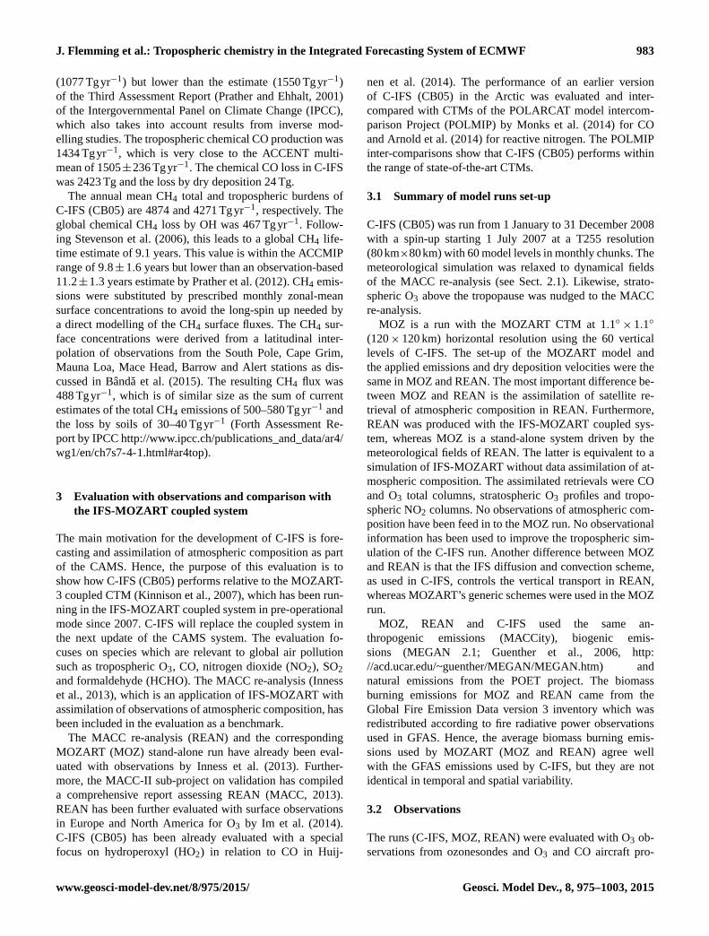
The annual mean CH4 total and tropospheric burdens of
C-IFS (CB05) are 4874 and 4271 Tgyr−1, respectively. The
global chemical CH4 loss by OH was 467 Tgyr−1. Follow-
ing Stevenson et al. (2006), this leads to a global CH4 life-
time estimate of 9.1 years. This value is within the ACCMIP
range of 9.8± 1.6 years but lower than an observation-based
11.2±1.3 years estimate by Prather et al. (2012). CH4 emis-
sions were substituted by prescribed monthly zonal-mean
surface concentrations to avoid the long-spin up needed by
a direct modelling of the CH4 surface fluxes. The CH4 sur-
face concentrations were derived from a latitudinal inter-
polation of observations from the South Pole, Cape Grim,
Mauna Loa, Mace Head, Barrow and Alert stations as dis-
cussed in Bânda et al. (2015). The resulting CH4 flux was
488 Tgyr−1, which is of similar size as the sum of current
estimates of the total CH4 emissions of 500–580 Tgyr−1 and
the loss by soils of 30–40 Tgyr−1 (Forth Assessment Re-
port by IPCC http://www.ipcc.ch/publications_and_data/ar4/
wg1/en/ch7s7-4-1.html#ar4top).
3 Evaluation with observations and comparison with
the IFS-MOZART coupled system
The main motivation for the development of C-IFS is fore-
casting and assimilation of atmospheric composition as part
of the CAMS. Hence, the purpose of this evaluation is to
show how C-IFS (CB05) performs relative to the MOZART-
3 coupled CTM (Kinnison et al., 2007), which has been run-
ning in the IFS-MOZART coupled system in pre-operational
mode since 2007. C-IFS will replace the coupled system in
the next update of the CAMS system. The evaluation fo-
cuses on species which are relevant to global air pollution
such as tropospheric O3, CO, nitrogen dioxide (NO2), SO2
and formaldehyde (HCHO). The MACC re-analysis (Inness
et al., 2013), which is an application of IFS-MOZART with
assimilation of observations of atmospheric composition, has
been included in the evaluation as a benchmark.
The MACC re-analysis (REAN) and the corresponding
MOZART (MOZ) stand-alone run have already been eval-
uated with observations by Inness et al. (2013). Further-
more, the MACC-II sub-project on validation has compiled
a comprehensive report assessing REAN (MACC, 2013).
REAN has been further evaluated with surface observations
in Europe and North America for O3 by Im et al. (2014).
C-IFS (CB05) has been already evaluated with a special
focus on hydroperoxyl (HO2) in relation to CO in Huij-
nen et al. (2014). The performance of an earlier version
of C-IFS (CB05) in the Arctic was evaluated and inter-
compared with CTMs of the POLARCAT model intercom-
parison Project (POLMIP) by Monks et al. (2014) for CO
and Arnold et al. (2014) for reactive nitrogen. The POLMIP
inter-comparisons show that C-IFS (CB05) performs within
the range of state-of-the-art CTMs.
3.1 Summary of model runs set-up
C-IFS (CB05) was run from 1 January to 31 December 2008
with a spin-up starting 1 July 2007 at a T255 resolution
(80km×80km) with 60 model levels in monthly chunks. The
meteorological simulation was relaxed to dynamical fields
of the MACC re-analysis (see Sect. 2.1). Likewise, strato-
spheric O3 above the tropopause was nudged to the MACC
re-analysis.
MOZ is a run with the MOZART CTM at 1.1◦× 1.1◦
(120× 120 km) horizontal resolution using the 60 vertical
levels of C-IFS. The set-up of the MOZART model and
the applied emissions and dry deposition velocities were the
same in MOZ and REAN. The most important difference be-
tween MOZ and REAN is the assimilation of satellite re-
trieval of atmospheric composition in REAN. Furthermore,
REAN was produced with the IFS-MOZART coupled sys-
tem, whereas MOZ is a stand-alone system driven by the
meteorological fields of REAN. The latter is equivalent to a
simulation of IFS-MOZART without data assimilation of at-
mospheric composition. The assimilated retrievals were CO
and O3 total columns, stratospheric O3 profiles and tropo-
spheric NO2 columns. No observations of atmospheric com-
position have been feed in to the MOZ run. No observational
information has been used to improve the tropospheric sim-
ulation of the C-IFS run. Another difference between MOZ
and REAN is that the IFS diffusion and convection scheme,
as used in C-IFS, controls the vertical transport in REAN,
whereas MOZART’s generic schemes were used in the MOZ
run.
MOZ, REAN and C-IFS used the same an-
thropogenic emissions (MACCity), biogenic emis-
sions (MEGAN 2.1; Guenther et al., 2006, http:
//acd.ucar.edu/~guenther/MEGAN/MEGAN.htm) and
natural emissions from the POET project. The biomass
burning emissions for MOZ and REAN came from the
Global Fire Emission Data version 3 inventory which was
redistributed according to fire radiative power observations
used in GFAS. Hence, the average biomass burning emis-
sions used by MOZART (MOZ and REAN) agree well
with the GFAS emissions used by C-IFS, but they are not
identical in temporal and spatial variability.
3.2 Observations
The runs (C-IFS, MOZ, REAN) were evaluated with O3 ob-
servations from ozonesondes and O3 and CO aircraft pro-
www.geosci-model-dev.net/8/975/2015/ Geosci. Model Dev., 8, 975–1003, 2015
984 J. Flemming et al.: Tropospheric chemistry in the Integrated Forecasting System of ECMWF
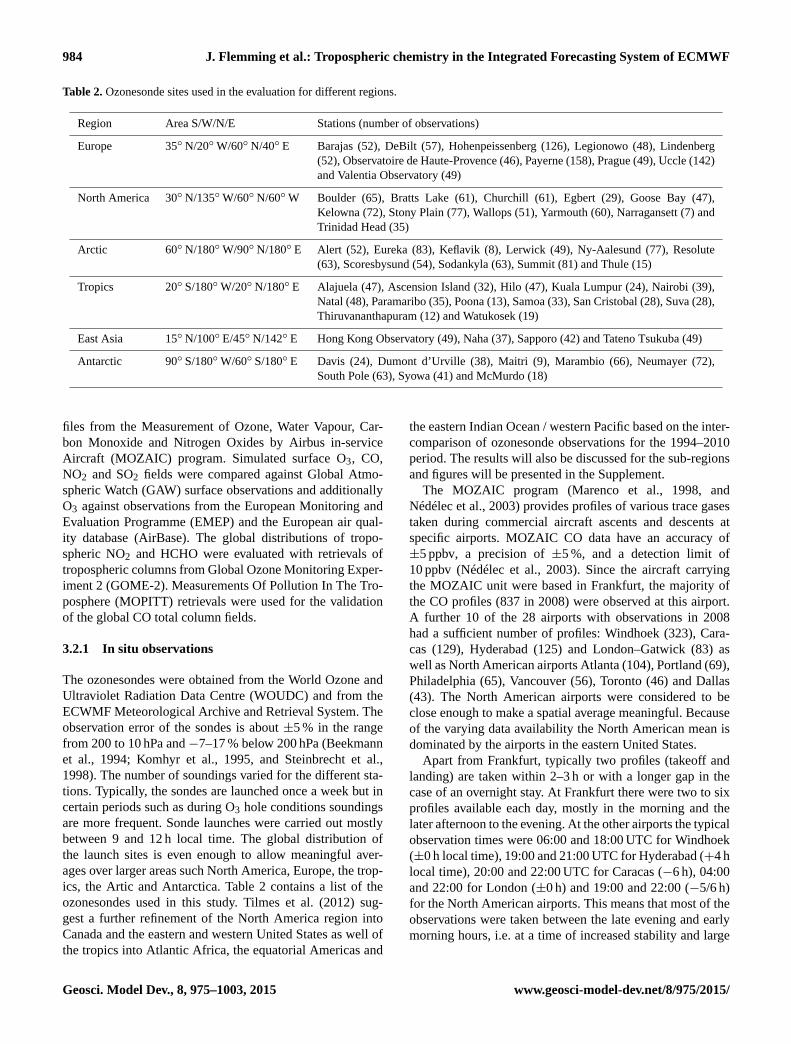
Table 2. Ozonesonde sites used in the evaluation for different regions.
Region Area S/W/N/E Stations (number of observations)
Europe 35◦ N/20◦W/60◦ N/40◦ E Barajas (52), DeBilt (57), Hohenpeissenberg (126), Legionowo (48), Lindenberg
(52), Observatoire de Haute-Provence (46), Payerne (158), Prague (49), Uccle (142)
and Valentia Observatory (49)
North America 30◦ N/135◦W/60◦ N/60◦W Boulder (65), Bratts Lake (61), Churchill (61), Egbert (29), Goose Bay (47),
Kelowna (72), Stony Plain (77), Wallops (51), Yarmouth (60), Narragansett (7) and
Trinidad Head (35)
Arctic 60◦ N/180◦W/90◦ N/180◦ E Alert (52), Eureka (83), Keflavik (8), Lerwick (49), Ny-Aalesund (77), Resolute
(63), Scoresbysund (54), Sodankyla (63), Summit (81) and Thule (15)
Tropics 20◦ S/180◦W/20◦ N/180◦ E Alajuela (47), Ascension Island (32), Hilo (47), Kuala Lumpur (24), Nairobi (39),
Natal (48), Paramaribo (35), Poona (13), Samoa (33), San Cristobal (28), Suva (28),
Thiruvananthapuram (12) and Watukosek (19)
East Asia 15◦ N/100◦ E/45◦ N/142◦ E Hong Kong Observatory (49), Naha (37), Sapporo (42) and Tateno Tsukuba (49)
Antarctic 90◦ S/180◦W/60◦ S/180◦ E Davis (24), Dumont d’Urville (38), Maitri (9), Marambio (66), Neumayer (72),
South Pole (63), Syowa (41) and McMurdo (18)
files from the Measurement of Ozone, Water Vapour, Car-
bon Monoxide and Nitrogen Oxides by Airbus in-service
Aircraft (MOZAIC) program. Simulated surface O3, CO,
NO2 and SO2 fields were compared against Global Atmo-
spheric Watch (GAW) surface observations and additionally
O3 against observations from the European Monitoring and
Evaluation Programme (EMEP) and the European air qual-
ity database (AirBase). The global distributions of tropo-
spheric NO2 and HCHO were evaluated with retrievals of
tropospheric columns from Global Ozone Monitoring Exper-
iment 2 (GOME-2). Measurements Of Pollution In The Tro-
posphere (MOPITT) retrievals were used for the validation
of the global CO total column fields.
3.2.1 In situ observations
The ozonesondes were obtained from the World Ozone and
Ultraviolet Radiation Data Centre (WOUDC) and from the
ECWMF Meteorological Archive and Retrieval System. The
observation error of the sondes is about ±5 % in the range
from 200 to 10 hPa and −7–17 % below 200 hPa (Beekmann
et al., 1994; Komhyr et al., 1995, and Steinbrecht et al.,
1998). The number of soundings varied for the different sta-
tions. Typically, the sondes are launched once a week but in
certain periods such as during O3 hole conditions soundings
are more frequent. Sonde launches were carried out mostly
between 9 and 12 h local time. The global distribution of
the launch sites is even enough to allow meaningful aver-
ages over larger areas such North America, Europe, the trop-
ics, the Artic and Antarctica. Table 2 contains a list of the
ozonesondes used in this study. Tilmes et al. (2012) sug-
gest a further refinement of the North America region into
Canada and the eastern and western United States as well of
the tropics into Atlantic Africa, the equatorial Americas and
the eastern Indian Ocean / western Pacific based on the inter-
comparison of ozonesonde observations for the 1994–2010
period. The results will also be discussed for the sub-regions
and figures will be presented in the Supplement.
The MOZAIC program (Marenco et al., 1998, and
Nédélec et al., 2003) provides profiles of various trace gases
taken during commercial aircraft ascents and descents at
specific airports. MOZAIC CO data have an accuracy of
±5 ppbv, a precision of ±5 %, and a detection limit of
10 ppbv (Nédélec et al., 2003). Since the aircraft carrying
the MOZAIC unit were based in Frankfurt, the majority of
the CO profiles (837 in 2008) were observed at this airport.
A further 10 of the 28 airports with observations in 2008
had a sufficient number of profiles: Windhoek (323), Cara-
cas (129), Hyderabad (125) and London–Gatwick (83) as
well as North American airports Atlanta (104), Portland (69),
Philadelphia (65), Vancouver (56), Toronto (46) and Dallas
(43). The North American airports were considered to be
close enough to make a spatial average meaningful. Because
of the varying data availability the North American mean is
dominated by the airports in the eastern United States.
Apart from Frankfurt, typically two profiles (takeoff and
landing) are taken within 2–3 h or with a longer gap in the
case of an overnight stay. At Frankfurt there were two to six
profiles available each day, mostly in the morning and the
later afternoon to the evening. At the other airports the typical
observation times were 06:00 and 18:00 UTC for Windhoek
(±0 h local time), 19:00 and 21:00 UTC for Hyderabad (+4 h
local time), 20:00 and 22:00 UTC for Caracas (−6 h), 04:00
and 22:00 for London (±0 h) and 19:00 and 22:00 (−5/6 h)
for the North American airports. This means that most of the
observations were taken between the late evening and early
morning hours, i.e. at a time of increased stability and large
Geosci. Model Dev., 8, 975–1003, 2015 www.geosci-model-dev.net/8/975/2015/

J. Flemming et al.: Tropospheric chemistry in the Integrated Forecasting System of ECMWF 985
CO vertical gradients close to the surface. Only the observa-
tions at Caracas (afternoon) and to some extent in Frankfurt
represent a more mixed day-time boundary layer. The mod-
elled column profile was obtained at the middle between the
start and end times of the profile observation and no consid-
eration was given to the horizontal movement of the aircraft.
The model columns were interpolated in time between two
subsequent output time steps.
The global atmospheric watch (GAW) program of the
World Meteorological Organization is a network for mainly
surface based observations (WMO, 2007). The data were re-
trieved from the World Data Centre for Greenhouse Gases
(http://ds.data.jma.go.jp/gmd/wdcgg/). The GAW observa-
tions represent the global background away from the main
polluted areas. Often, the GAW observation sites are lo-
cated on mountains, which makes it necessary to select a
model level different from the lowest model level for a sound
comparison with the model. In this study the procedure de-
scribed in Flemming et al. (2009b) is applied to determine
the model level, which is based on the difference between a
high-resolution orography and the actual station height. The
data coverage for CO and O3 was global, whereas for SO2
and NO2, only a few observations in Europe were available
at the data repository.
The Airbase and EMEP databases host operational air
quality observations from different national European net-
works. All EMEP stations are located in rural areas, while
Airbase stations are designed to monitor local pollution.
Many AirBase observations may therefore not be representa-
tive of a global model with a horizontal resolution of 80 km.
However, stations of rural regime may capture the larger-
scale signal, in particular for O3, which is spatially well cor-
related (Flemming et al., 2005). The EMEP observations and
the rural Airbase O3 observations were used for the evalua-
tion over Europe.
3.2.2 Satellite retrievals
Satellite retrievals of atmospheric composition are more
widely used to evaluate model results. Satellite data provide
good horizontal coverage but have limitation with respect
to the vertical resolution and signal from the lowest atmo-
spheric levels. Furthermore, satellite observations are only
possible at the specific overpass time, and they can be dis-
turbed by the presence of clouds and surface properties. De-
pending on the instrument type global coverage is achieved
in several days.
Day-time CO total column retrievals from MOPITT, ver-
sion 6 (Deeter, 2013), and retrievals of tropospheric columns
of NO2 (IUP-UB v0.7, Richter et al., 2005) and of HCHO
(IUP-UB v1.0; Wittrock et al., 2006) from GOME-2 (Callies
et al., 2000) have been used for the evaluation. The retrievals
were averaged to monthly means values to reduce the random
retrieval error.
MOPITT is a multispectral thermal infrared (TIR)/near
infrared (NIR) instrument onboard the TERRA satellite
with a pixel resolution of 22 km. TERRA’s local equato-
rial crossing time is approximately 10:30 a.m. The MO-
PITT CO level 2 pixels were binned within 1× 1◦ within
each month. Deeter et al. (2013) report a bias of about
+0.08× 10¹⁸ moleccm−2 and a standard deviation (SD) of
the error of 0.19× 10¹⁸ moleccm−2 for the TIR/NIR prod-
uct version 5. This is equivalent to a bias of about 4 % and
a SD of 10 % respectively assuming typical observations of
2.0× 10¹⁸ moleccm−2. For the calculation of the simulated
CO total column, the a priori profile in combination with the
averaging kernels (AK) of the retrievals was applied. They
have the largest values between 300 and 800 hPa. The AK
have been applied to ensure that the difference between re-
trieval and the AK-weighted model column is independent of
the a priori CO profiles used in the retrieval. One should note
however, that the AK-weighted column is not equivalent to
the modelled atmospheric CO burden anymore.
GOME-2 is a ultra violet-visible (UV-VIS) and NIR sen-
sor designed to provide global observations of atmospheric
trace gases. GOME-2 flies in a sun-synchronous orbit with
an equatorial crossing time of 09:30 LT in descending mode
and has a footprint of 40× 80 km. Here, tropospheric verti-
cal columns of NO2 and HCHO have been computed using
a three step approach. First, the differential optical absorp-
tion spectroscopy (DOAS; Platt, 1994) method is applied to
measured spectra which yields the total slant column. The
DOAS method is applied in a 425–497 nm wavelength win-
dow (Richter et al., 2011) for NO2. and between 337 and
353 nm for HCHO (Vrekoussis et al., 2010). Second, the
reference sector approach is applied to total slant columns
for stratospheric correction. In a last step, tropospheric slant
columns are converted to tropospheric vertical columns by
applying an air mass factor. Only data with cloud fractions
smaller than 0.2 according to the FRESCO cloud database
(Wang et al., 2008) are used here. Furthermore, retrievals are
limited to maximum solar zenith angles of 85◦ for NO2 and
60◦ for HCHO. Uncertainties in NO2 satellite retrievals are
large and depend on the region and season. Winter values at
middle and high latitudes are usually associated with larger
error margins. As a rough estimate, systematic uncertainties
in regions with significant pollution are of the order of 20–
30 %. As the HCHO retrieval is performed in the UV part of
the spectrum where less light is available and the HCHO ab-
sorption signal is smaller than that of NO2, the uncertainty of
monthly mean HCHO columns is relatively large (20–40 %)
and both noise and systematic offsets have an influence on
the results. However, absolute values and seasonality are re-
trieved more accurately over HCHO hotspots.
For comparison to GOME-2 data, model data are verti-
cally integrated without applying AK to tropospheric ver-
tical columns of NO2 and HCHO, interpolated to satellite
observation time and then sampled to match the location of
available cloud free satellite data, which has been gridded to
www.geosci-model-dev.net/8/975/2015/ Geosci. Model Dev., 8, 975–1003, 2015

986 J. Flemming et al.: Tropospheric chemistry in the Integrated Forecasting System of ECMWF
Figure 2. Tropospheric ozone volume mixing ratios (ppb) over Europe (left) and North America (middle) and East Asia (right) averaged in
the pressure ranges 1000–700 hPa (bottom), 700–400 hPa (middle) and 400–200 hPa (top) observed by ozonesondes (black) and simulated
by C-IFS (red), MOZ (blue) and REAN (green) in 2008.
match the model resolution. The resulting daily files are then
averaged over months for both satellite and model data to
reduce the noise.
3.3 Tropospheric ozone
Figure 2 shows the monthly means of O3 volume mixing
ratios in the pressure ranges surface to 700 hPa (lower tro-
posphere, LT) 700–400 hPa (middle troposphere, MT) and
400–200 hPa (upper troposphere UT) observed by sondes
and averaged over Europe, North America and East Asia.
Figure 3 shows the same as Fig. 2 for the tropics, Arctic
and Antarctica. A more detailed breakdown of North Amer-
ica (Canada, eastern and western United States) and the
tropics (Atlantic Africa, equatorial Americas and eastern In-
dian Ocean/western Pacific) following Tilmes et al. (2012) is
presented in the supplement. The observations have a pro-
nounced spring maximum for UT O3 over Europe, North
America and East Asia and a more gradually developing
maximum in late spring and summer in MT and LT. The
LT seasonal cycle is well re-produced in all runs for the ar-
eas of the Northern Hemisphere (NH). In Europe, REAN
tends to overestimate by about 5 ppb where the C-IFS and
MOZ have almost no bias before the annual maximum in
May apart from a small negative bias in spring. Later in the
year, C-IFS tends to overestimate in autumn, whereas MOZ
overestimates more in late summer. In MT over Europe, C-
IFS agrees slightly better with the observations than MOZ.
MOZ overestimates in winter and spring and this overesti-
mation is more prominent in the UT, where MOZ is biased
high throughout the year. This overestimation in UT is high-
est in spring, where it can be 25 % and more. These findings
show that data assimilation in REAN improved UT O3 con-
siderably but had only little influence in LT and MT. The
overestimation of MOZ in UT seems to be caused by in-
creased stratospheric O3 rather than a more efficient transport
as lower stratospheric O3 was overestimated in MOZ. Note
that stratospheric ozone in C-IFS was nudged to the MACC
re-analysis (see Sect. 3.1) but good agreement of C-IFS with
observation in UT in all three regions is also present in a run
without nudging to stratospheric O3. It is therefore not only a
consequence of the use of assimilated observations in C-IFS
(CB05).
Geosci. Model Dev., 8, 975–1003, 2015 www.geosci-model-dev.net/8/975/2015/
J. Flemming et al.: Tropospheric chemistry in the Integrated Forecasting System of ECMWF 987
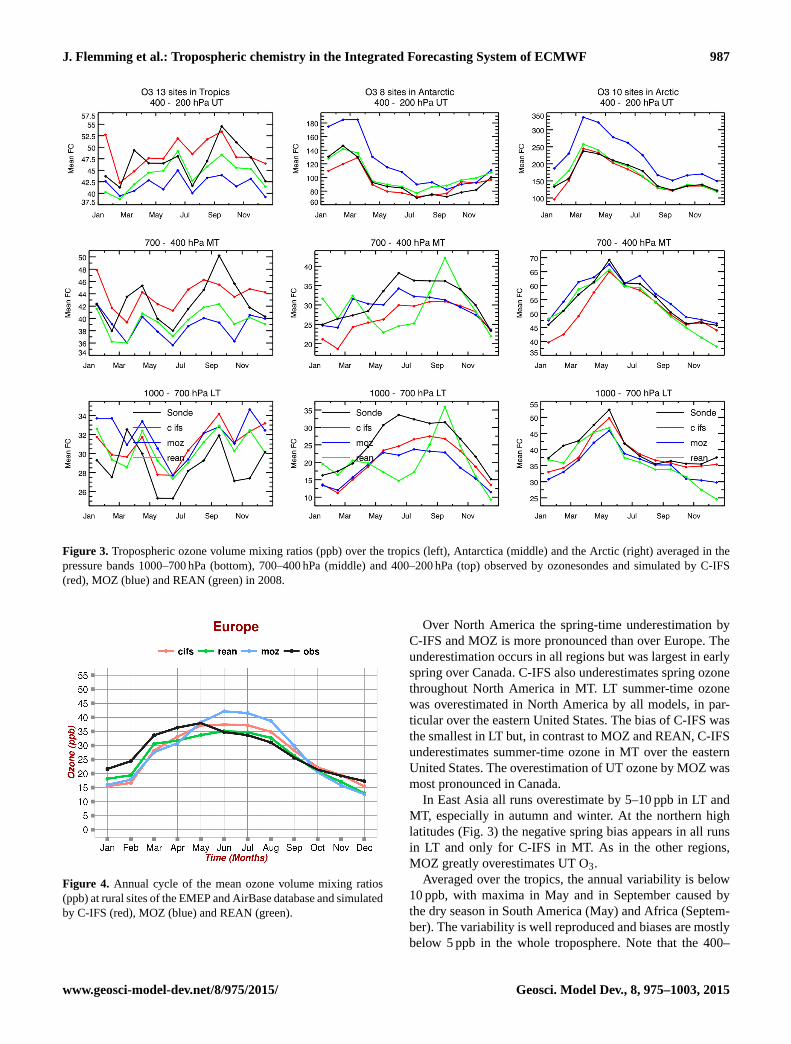
Figure 3. Tropospheric ozone volume mixing ratios (ppb) over the tropics (left), Antarctica (middle) and the Arctic (right) averaged in the
pressure bands 1000–700 hPa (bottom), 700–400 hPa (middle) and 400–200 hPa (top) observed by ozonesondes and simulated by C-IFS
(red), MOZ (blue) and REAN (green) in 2008.
Figure 4. Annual cycle of the mean ozone volume mixing ratios
(ppb) at rural sites of the EMEP and AirBase database and simulated
by C-IFS (red), MOZ (blue) and REAN (green).
Over North America the spring-time underestimation by
C-IFS and MOZ is more pronounced than over Europe. The
underestimation occurs in all regions but was largest in early
spring over Canada. C-IFS also underestimates spring ozone
throughout North America in MT. LT summer-time ozone
was overestimated in North America by all models, in par-
ticular over the eastern United States. The bias of C-IFS was
the smallest in LT but, in contrast to MOZ and REAN, C-IFS
underestimates summer-time ozone in MT over the eastern
United States. The overestimation of UT ozone by MOZ was
most pronounced in Canada.
In East Asia all runs overestimate by 5–10 ppb in LT and
MT, especially in autumn and winter. At the northern high
latitudes (Fig. 3) the negative spring bias appears in all runs
in LT and only for C-IFS in MT. As in the other regions,
MOZ greatly overestimates UT O3.
Averaged over the tropics, the annual variability is below
10 ppb, with maxima in May and in September caused by
the dry season in South America (May) and Africa (Septem-
ber). The variability is well reproduced and biases are mostly
below 5 ppb in the whole troposphere. Note that the 400–
www.geosci-model-dev.net/8/975/2015/ Geosci. Model Dev., 8, 975–1003, 2015

988 J. Flemming et al.: Tropospheric chemistry in the Integrated Forecasting System of ECMWF
Figure 5. Diurnal cycle of surface ozone volume mixing ratios (ppb) over Europe in winter (top, left), spring (top, right), summer (bottom,
left) and autumn (bottom, right) at the rural site of the EMEP and AirBase database and simulated by C-IFS (red), MOZ (blue) and REAN
(green).
200 hPa range (UT) in the tropics is less influenced by the
stratosphere because of the higher tropopause. C-IFS had
smaller biases because of lower values in LT and higher
values in MT and UT than MOZ. A more detailed analy-
sis for different tropical regions shows that the seasonality is
well captured by all models over Atlantic Africa, equatorial
America and the eastern Indian Ocean / western Pacific in
all three tropospheric levels. However, the strong observed
monthly anomalies (an observation glitch by one station) in
equatorial America in March and September were underesti-
mated by up to 20 ppb in all tropospheric levels.
Over the Arctic, C-IFS and MOZ reproduce the seasonal
cycle, which peaks in late spring, but generally underestimate
the observations in LT. C-IFS had a smaller bias in LT than
MOZ but had a larger negative bias in MT. The biggest im-
provement in C-IFS w.r.t. to MOZ occurred at the surface
in Antarctica as the biases compared to the GAW surface
observations were greatly reduced. Notably, the assimilation
(REAN) led to increased biases for LT and MT O3, in par-
ticular during polar night when UV satellite observations are
not available, as already discussed in Flemming et al. (2011).
The ability of the models to simulate O3 near the surface is
tested with rural AirBase and EMEP stations (see Sect. 3.2).
Figure 4 shows monthly means and Fig. 5 the average diurnal
cycle in different seasons in Europe. All runs underestimate
monthly mean O3 in spring and winter and overestimate it
in late summer and autumn. The overestimation in summer
was largest in MOZ. The recently reported (Val Martin at al.,
2014) missing coupling of the leaf area index to the leaf and
stomatal vegetation resistance in the calculation of dry de-
position velocities could be an explanation of the MOZ bias.
While the overestimation appeared also with respect to the
ozonesondes in LT (see Fig. 2, left), the spring-time underes-
timation was less pronounced in LT.
The comparison of the diurnal cycle with observations
(Fig. 5) shows that C-IFS produced a more realistic diurnal
cycle than the MOZART model. The diurnal variability sim-
ulated by the MOZART model is much less pronounced than
the observations suggest. The diurnal cycles of C-IFS and
REAN were similar. This finding can be explained by the fact
that C-IFS and REAN use the IFS diffusion scheme, whereas
MOZART applies the diffusion scheme of the MOZART
CTM.
The negative bias of C-IFS in winter and spring seems
mainly caused by an underestimation of the night-time val-
ues, whereas the overestimations of the summer and autumn
average values in C-IFS were caused by an overestimation
of the day-time values. However, the overestimation of the
summer night-time values by MOZART seems to be a strong
contribution to the average overestimation in this season.
Geosci. Model Dev., 8, 975–1003, 2015 www.geosci-model-dev.net/8/975/2015/
J. Flemming et al.: Tropospheric chemistry in the Integrated Forecasting System of ECMWF 989
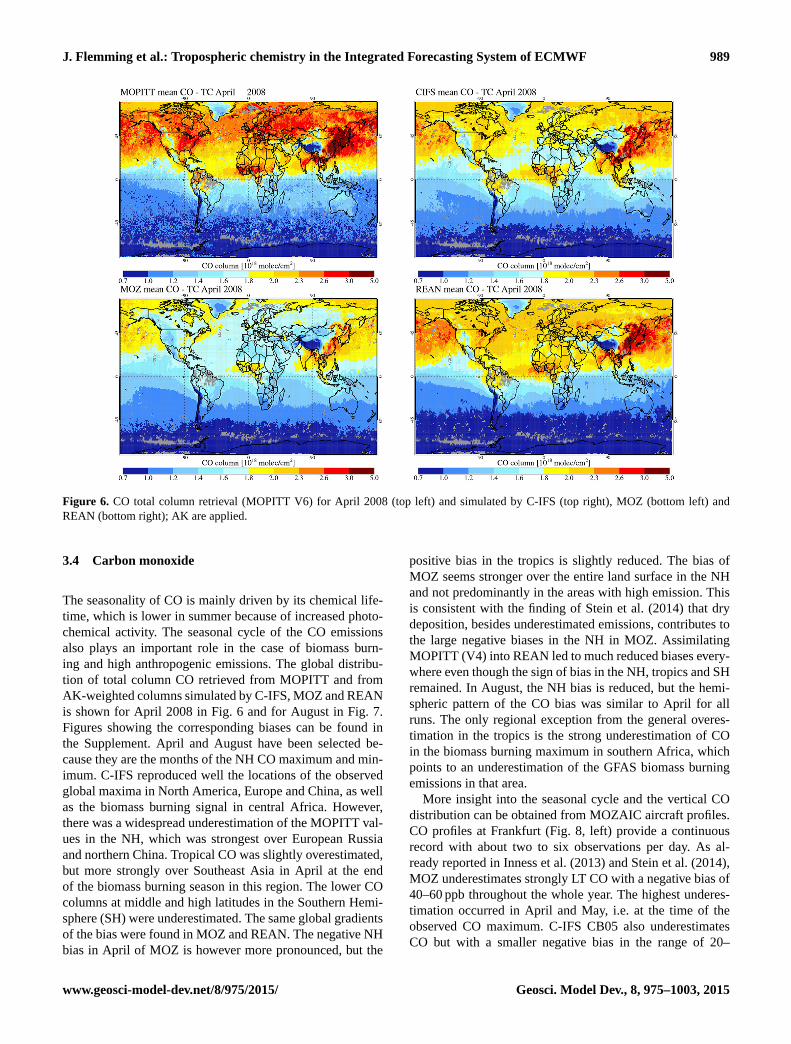
Figure 6. CO total column retrieval (MOPITT V6) for April 2008 (top left) and simulated by C-IFS (top right), MOZ (bottom left) and
REAN (bottom right); AK are applied.
3.4 Carbon monoxide
The seasonality of CO is mainly driven by its chemical life-
time, which is lower in summer because of increased photo-
chemical activity. The seasonal cycle of the CO emissions
also plays an important role in the case of biomass burn-
ing and high anthropogenic emissions. The global distribu-
tion of total column CO retrieved from MOPITT and from
AK-weighted columns simulated by C-IFS, MOZ and REAN
is shown for April 2008 in Fig. 6 and for August in Fig. 7.
Figures showing the corresponding biases can be found in
the Supplement. April and August have been selected be-
cause they are the months of the NH CO maximum and min-
imum. C-IFS reproduced well the locations of the observed
global maxima in North America, Europe and China, as well
as the biomass burning signal in central Africa. However,
there was a widespread underestimation of the MOPITT val-
ues in the NH, which was strongest over European Russia
and northern China. Tropical CO was slightly overestimated,
but more strongly over Southeast Asia in April at the end
of the biomass burning season in this region. The lower CO
columns at middle and high latitudes in the Southern Hemi-
sphere (SH) were underestimated. The same global gradients
of the bias were found in MOZ and REAN. The negative NH
bias in April of MOZ is however more pronounced, but the
positive bias in the tropics is slightly reduced. The bias of
MOZ seems stronger over the entire land surface in the NH
and not predominantly in the areas with high emission. This
is consistent with the finding of Stein et al. (2014) that dry
deposition, besides underestimated emissions, contributes to
the large negative biases in the NH in MOZ. Assimilating
MOPITT (V4) into REAN led to much reduced biases every-
where even though the sign of bias in the NH, tropics and SH
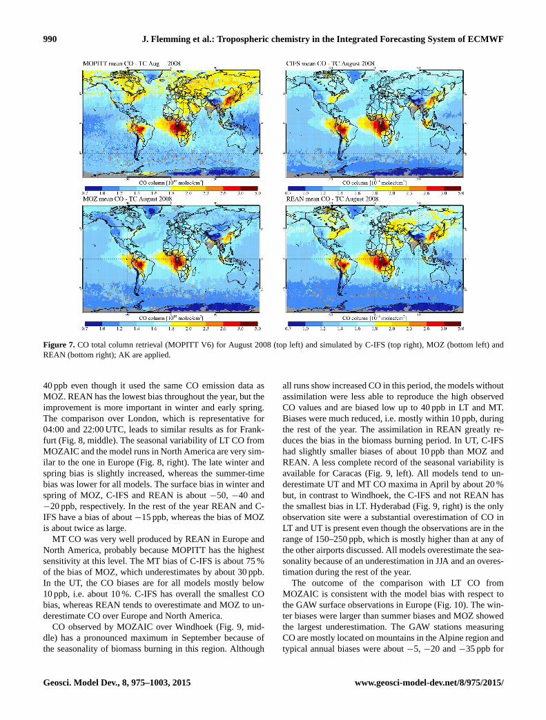
remained. In August, the NH bias is reduced, but the hemi-
spheric pattern of the CO bias was similar to April for all
runs. The only regional exception from the general overes-
timation in the tropics is the strong underestimation of CO
in the biomass burning maximum in southern Africa, which
points to an underestimation of the GFAS biomass burning
emissions in that area.
More insight into the seasonal cycle and the vertical CO
distribution can be obtained from MOZAIC aircraft profiles.
CO profiles at Frankfurt (Fig. 8, left) provide a continuous
record with about two to six observations per day. As al-
ready reported in Inness et al. (2013) and Stein et al. (2014),
MOZ underestimates strongly LT CO with a negative bias of
40–60 ppb throughout the whole year. The highest underes-
timation occurred in April and May, i.e. at the time of the
observed CO maximum. C-IFS CB05 also underestimates
CO but with a smaller negative bias in the range of 20–
www.geosci-model-dev.net/8/975/2015/ Geosci. Model Dev., 8, 975–1003, 2015
990 J. Flemming et al.: Tropospheric chemistry in the Integrated Forecasting System of ECMWF
Figure 7. CO total column retrieval (MOPITT V6) for August 2008 (top left) and simulated by C-IFS (top right), MOZ (bottom left) and
REAN (bottom right); AK are applied.
40 ppb even though it used the same CO emission data as
MOZ. REAN has the lowest bias throughout the year, but the
improvement is more important in winter and early spring.
The comparison over London, which is representative for
04:00 and 22:00 UTC, leads to similar results as for Frank-
furt (Fig. 8, middle). The seasonal variability of LT CO from
MOZAIC and the model runs in North America are very sim-
ilar to the one in Europe (Fig. 8, right). The late winter and
spring bias is slightly increased, whereas the summer-time
bias was lower for all models. The surface bias in winter and
spring of MOZ, C-IFS and REAN is about −50, −40 and
−20 ppb, respectively. In the rest of the year REAN and C-
IFS have a bias of about −15 ppb, whereas the bias of MOZ
is about twice as large.
MT CO was very well produced by REAN in Europe and
North America, probably because MOPITT has the highest
sensitivity at this level. The MT bias of C-IFS is about 75 %
of the bias of MOZ, which underestimates by about 30 ppb.
In the UT, the CO biases are for all models mostly below
10 ppb, i.e. about 10 %. C-IFS has overall the smallest CO
bias, whereas REAN tends to overestimate and MOZ to un-
derestimate CO over Europe and North America.
CO observed by MOZAIC over Windhoek (Fig. 9, mid-
dle) has a pronounced maximum in September because of
the seasonality of biomass burning in this region. Although
all runs show increased CO in this period, the models without
assimilation were less able to reproduce the high observed
CO values and are biased low up to 40 ppb in LT and MT.
Biases were much reduced, i.e. mostly within 10 ppb, during
the rest of the year. The assimilation in REAN greatly re-
duces the bias in the biomass burning period. In UT, C-IFS
had slightly smaller biases of about 10 ppb than MOZ and
REAN. A less complete record of the seasonal variability is
available for Caracas (Fig. 9, left). All models tend to un-
derestimate UT and MT CO maxima in April by about 20 %
but, in contrast to Windhoek, the C-IFS and not REAN has
the smallest bias in LT. Hyderabad (Fig. 9, right) is the only
observation site were a substantial overestimation of CO in
LT and UT is present even though the observations are in the
range of 150–250 ppb, which is mostly higher than at any of
the other airports discussed. All models overestimate the sea-
sonality because of an underestimation in JJA and an overes-
timation during the rest of the year.
The outcome of the comparison with LT CO from
MOZAIC is consistent with the model bias with respect to
the GAW surface observations in Europe (Fig. 10). The win-
ter biases were larger than summer biases and MOZ showed
the largest underestimation. The GAW stations measuring
CO are mostly located on mountains in the Alpine region and
typical annual biases were about −5, −20 and −35 ppb for
Geosci. Model Dev., 8, 975–1003, 2015 www.geosci-model-dev.net/8/975/2015/

J. Flemming et al.: Tropospheric chemistry in the Integrated Forecasting System of ECMWF 991
Figure 8. CO volume mixing ratios (ppb) over Frankfurt (left), London (middle) and North America (left, averaged over six airports) averaged
in the pressure bands 1000–700 hPa (bottom), 700–400 hPa (middle) and 400–200 hPa (top) observed by MOZAIC and simulated by C-IFS
(red), MOZ (blue) and REAN (green) in 2008.
REAN, C-IFS and MOZ, respectively. The negative biases of
stations in flatter terrain such as Kollumerward tended to be
larger.
3.5 Nitrogen dioxide
The global maxima of NO2 are located in areas of high an-
thropogenic and biomass burning NO emissions. The global
annual distribution of annual tropospheric columns retrieved
from the GOME-2 instrument and simulated by the models
is shown in Fig. 11. C-IFS, MOZ and REAN showed a very
similar distribution, which can be explained by that fact that
the same NO emission data were used in all runs. The global
patterns of the modelled fields resemble the observed annual
patterns to a large extent. But the models tend to underesti-
mate the high observed values in East Asia and Europe and
also simulate too little NO2 in larger areas of medium ob-
served NO2 levels in Asia and central Africa as well as in
the outflow areas over the western Atlantic and western Pa-
cific Ocean. This could mean that NO emissions in the most
polluted areas are too low but also that the simulated lifetime
of NO2 is too short. Furthermore, an insufficient simulation
of NOx reservoir species such as PAN and the lack of alkyl
nitrates in CB05 might be the reason for the underestimation.
The validation of the seasonality of NO2 (Fig. 12) for
different regions and months shows that tropospheric NO2
columns over Europe, North America, South Africa and East
Asia are reasonably reproduced. The models tend to under-
estimate tropospheric columns over Europe in summer (see
Table 2 for area descriptions). However, the evaluation with
GAW surface stations mainly from central and eastern Eu-
rope (Fig. 13) revealed an overestimation by all models in
winter and a small overestimation in summer for REAN and
C-IFS. All runs significantly underestimate the annual cycle
of the GOME-2 NO2 tropospheric columns over East Asia.
The winter-time values are only half of the observations,
whereas in summer, models agree well with observations. In
southern Africa (20/0◦ S/15/15◦W), the models overestimate
the increased NO2 values in the biomass burning season by a
factor of 2 but show good agreement with observations in the
rest of the year. The overestimation during biomass burning
events could be related to the assumed NO emission factor.
www.geosci-model-dev.net/8/975/2015/ Geosci. Model Dev., 8, 975–1003, 2015
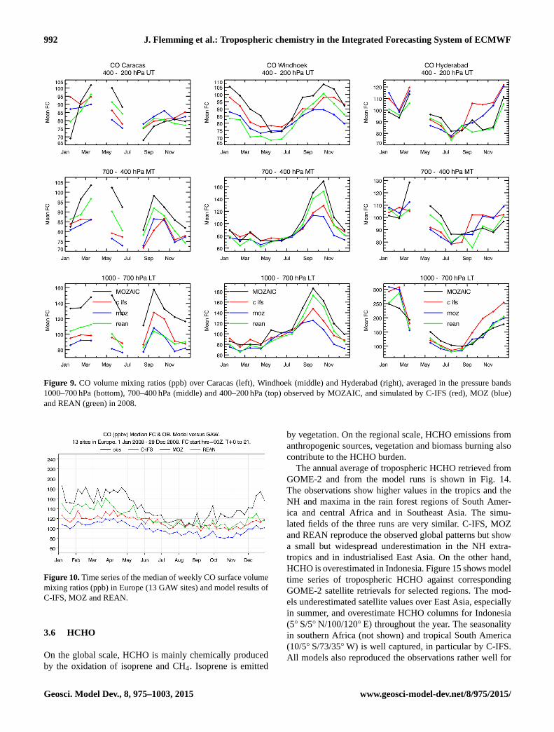
992 J. Flemming et al.: Tropospheric chemistry in the Integrated Forecasting System of ECMWF
Figure 9. CO volume mixing ratios (ppb) over Caracas (left), Windhoek (middle) and Hyderabad (right), averaged in the pressure bands
1000–700 hPa (bottom), 700–400 hPa (middle) and 400–200 hPa (top) observed by MOZAIC, and simulated by C-IFS (red), MOZ (blue)
and REAN (green) in 2008.
Figure 10. Time series of the median of weekly CO surface volume
mixing ratios (ppb) in Europe (13 GAW sites) and model results of
C-IFS, MOZ and REAN.
3.6 HCHO
On the global scale, HCHO is mainly chemically produced
by the oxidation of isoprene and CH4. Isoprene is emitted
by vegetation. On the regional scale, HCHO emissions from
anthropogenic sources, vegetation and biomass burning also
contribute to the HCHO burden.
The annual average of tropospheric HCHO retrieved from
GOME-2 and from the model runs is shown in Fig. 14.
The observations show higher values in the tropics and the
NH and maxima in the rain forest regions of South Amer-
ica and central Africa and in Southeast Asia. The simu-
lated fields of the three runs are very similar. C-IFS, MOZ
and REAN reproduce the observed global patterns but show
a small but widespread underestimation in the NH extra-
tropics and in industrialised East Asia. On the other hand,
HCHO is overestimated in Indonesia. Figure 15 shows model
time series of tropospheric HCHO against corresponding
GOME-2 satellite retrievals for selected regions. The mod-
els underestimated satellite values over East Asia, especially
in summer, and overestimate HCHO columns for Indonesia
(5◦ S/5◦ N/100/120◦ E) throughout the year. The seasonality
in southern Africa (not shown) and tropical South America
(10/5◦ S/73/35◦W) is well captured, in particular by C-IFS.
All models also reproduced the observations rather well for
Geosci. Model Dev., 8, 975–1003, 2015 www.geosci-model-dev.net/8/975/2015/

J. Flemming et al.: Tropospheric chemistry in the Integrated Forecasting System of ECMWF 993
Figure 11. NO2 tropospheric column retrieval (GOME-2) for 2008 (top left) and by C-IFS (top right), REAN (bottom right) and MOZ
(bottom left).
Figure 12. Time series of area-averaged tropospheric NO2 columns (1015 moleccm−2) from GOME-2 compared to model results of C-IFS
(CB05) (blue), MOZ (red) and REAN (green) for different regions.
www.geosci-model-dev.net/8/975/2015/ Geosci. Model Dev., 8, 975–1003, 2015

994 J. Flemming et al.: Tropospheric chemistry in the Integrated Forecasting System of ECMWF
Figure 13. Time series of the median of weekly surface NO2 vol-
ume mixing ratios (ppb) in Europe (20 GAW sites) and model re-
sults of C-IFS, MOZ and REAN.
the eastern United States (30/40◦ N/90/75◦W), but tend to
underestimate wintertime HCHO columns for this region.
3.7 Sulfur dioxide
SO2 was evaluated with available GAW surface observations
from central and eastern Europe. There were considerable
differences in the performance for individual stations often
caused by local effects not resolved by the models. To sum-
marise the evaluation for SO2, Fig. 16 shows the median of
weekly observed and modelled time series. REAN and MOZ
greatly exaggerated the seasonal cycle since the values in
winter were up to 8 times larger than the median of the ob-
servations. The summer values of the two runs were about
50 % higher than the observations. C-IFS followed better
the weak seasonality of the observations, but suffered from
a nearly constant bias of about 1 ppb (100 %), which was
much smaller than the bias of REAN and MOZ in winter, but
slightly higher in summer. Overall, the on-line integration of
C-IFS showed lower SO2 biases.
As no SO2 observations were assimilated in REAN and
identical SO2 emissions were used, the differences between
the runs were caused by differences in the simulation of verti-
cal mixing, sulfur chemistry and wet and dry deposition in C-
IFS and MOZART. The winter-time bias of REAN and MOZ
could be introduced by the diffusion scheme in MOZART.
3.8 Computational cost
The computational cost is an important factor for the oper-
ational applications in CAMS. The computational costs of
different configurations of IFS, C-IFS and IFS-MOZART are
given in Table 3. Computational cost is expressed in billing
units (BU) of the ECMWF IBM Power 7 super-computer.
BUs are proportional to the number of used central process-
ing units (CPU) times the simulation time.
The increase in cost because of the simulation of the CB05
chemistry with respect to an NWP run is a factor of about 4 at
resolutions T159 (110 km), T255 (80 km) and T511 (40 km).
C-IFS (CB05) is about 8 times more efficient than the IFS-
MOZART coupled system at a T159 resolution and about 15
times more at a T255 resolution. This strong relative increase
in cost of IFS-MOZART is caused by the increasing memory
requirements of the IFS at higher resolution, or also in data
assimilation mode. However, there is insufficient parallelism
in MOZART to exploit the larger number of CPUs for speed-
ing up the simulation of the coupled system.
C-IFS with the MOZART chemical mechanism, i.e. the
same chemistry scheme as in IFS-MOZART, is about 2
times and C-IFS with RACMOBUS 7 times more costly
than C-IFS (CB05) at a T159 resolution. Both the MOZART
and RACMOBUS schemes encompass a larger number of
species and reactions and include a full stratospheric chem-
istry scheme, which is missing in CB05. The overhead be-
cause of the doubled number of advected species in C-IFS
RACMOBUS and MOZART is however small because of the
efficiency of the SL advection scheme.
4 Summary and outlook
Modules for the simulation of atmospheric chemistry have
been implemented on-line in the Integrated Forecasting Sys-
tem (IFS) of ECMWF. The chemistry scheme complements
the already integrated modules for aerosol and greenhouse
gases as part of the IFS for atmospheric composition (C-IFS).
C-IFS for chemistry replaces the IFS-MOZART coupled sys-
tem for forecast and assimilation of reactive gases within the
pre-operational Copernicus Atmosphere Monitoring Service.
C-IFS applies the CB05 chemical mechanism, which de-
scribes tropospheric chemistry with 55 species and 126 re-
actions. C-IFS benefits from the detailed cloud and precip-
itation physics of the IFS for the calculation of wet deposi-
tion and lightning NO emission. Wet deposition modelling
is based on Jacob (2000) and accounts for the sub-grid-
scale distribution of clouds and precipitation. Dry deposition
is modelled using pre-calculated monthly mean dry deposi-
tion velocities following Wesely (1989) with a superimposed
diurnal cycle. Surface emissions and dry deposition fluxes
are applied as surface boundary conditions of the diffusion
scheme. Lightning emissions of NO can be calculated ei-
ther by cloud height (Price and Rind, 1993) or by convec-
tive precipitation (Meijer et al., 2001). The latter parameter-
isation was used in this study. The anthropogenic emissions
were taken from the MACCity inventory and biomass burn-
ing emissions from the GFAS data set for 2008.
An evaluation for the troposphere of a simulation in 2008
with C-IFS (CB05) and the MOZART CTM (MOZ) as
well as with the MACC re-analysis (REAN) was carried
out. The model results were compared against ozonesondes,
MOZAIC CO aircraft profiles, European surface observa-
tions of O3, CO, SO2 and NO2, and global satellite retrievals
of CO, NO2 and HCHO. The evaluation showed that C-IFS
Geosci. Model Dev., 8, 975–1003, 2015 www.geosci-model-dev.net/8/975/2015/

J. Flemming et al.: Tropospheric chemistry in the Integrated Forecasting System of ECMWF 995
Figure 14. HCHO tropospheric column retrieval (GOME-2) for 2008 (top left) and by C-IFS (top right), REAN (bottom right) and MOZ
(bottom left).
Figure 15. Time series of area-averaged tropospheric HCHO columns (1016 moleccm−2) from GOME-2 compared to model results of
C-IFS, MOZ and REAN for different regions.
www.geosci-model-dev.net/8/975/2015/ Geosci. Model Dev., 8, 975–1003, 2015

996 J. Flemming et al.: Tropospheric chemistry in the Integrated Forecasting System of ECMWF
Table 3. Computational cost (BU) of 24 h forecasts of different horizontal model resolutions (60 levels) and chemistry schemes of C-IFS,
IFS-MOZART and IFS, *not fully optimised.
Resolution IFS-MOZART C-IFS (MOZART)* C-IFS (MOCAGE)* C-IFS (CB05) IFS
T159 205 56 147 20 6
T255 1200 – – 55 12
T511 – – – 700 125
Figure 16. Time series of the median of weekly surface SO2 volume
mixing ratios (ppb) in Europe (21 GAW sites) and model results of
C-IFS, MOZ and REAN.
preforms better or with similar accuracy as MOZART and
is mostly of a similar quality as the MACC re-analysis. It
should be noted that satellite retrievals of CO, O3 and NO2
were assimilated into the MACC re-analysis to improve the
realism of the fields simulated by IFS-MOZART.
In comparison to MOZ, C-IFS (CB05) had smaller biases
(i) for CO in the Northern Hemisphere, (ii) for O3 in the up-
per troposphere and (iii) for winter-time SO2 at the surface in
Europe. Furthermore, the diurnal cycle of surface O3, tested
with rural European Air quality observations, showed greater
realism in the C-IFS simulation. As both models used the
same emission data, the improvements can be explained by
the differences in the chemical mechanism and the simula-
tion of wet and dry deposition. However, the improvements
in SO2 and the diurnal cycle of O3 are most probably caused
by the more consistent interplay of diffusion and sink and
sources processes in the on-line integrated C-IFS.
There is still room for improvement of C-IFS (CB05). It
underestimated surface O3 over Europe and North America
in spring and overestimated it in late summer and autumn.
CO was still underestimated by C-IFS in particular in Europe
and North America throughout the year but more in spring
and winter, and in the biomass burning season in Africa.
Winter-time tropospheric NO2 over China as retrieved from
the GOME-2 instrument was 2 times higher than the fields
modelled by C-IFS, MOZART and the MACC re-analysis.
Although only one chemical mechanism is described in the
paper, C-IFS is a model that can apply multiple chemistry
schemes. The implementation of the chemistry schemes of
CTMs MOCAGE and MOZART has technically been com-
pleted but further optimisation and evaluation is required.
Both schemes offer a description of stratospheric chemistry,
which is not included in the tropospheric scheme CB05.
For this reason it is intended to combine the CB05 mecha-
nism with the BASCOE stratospheric mechanism. An inter-
comparison of the performance of the different chemical
mechanism is planned.
It is foreseen to further improve the link between the
physics and chemistry packages in IFS. For example, the
detailed information from the IFS surface scheme will be
utilised for the calculation of dry deposition and biogenic
emissions. A first important step is to replace the climato-
logical dry deposition velocities with on-line calculated val-
ues. Furthermore, the impact of the simulated O3 fields, once
the stratospheric chemistry is fully implemented, on the IFS
radiation scheme and the corresponding feedback on the tem-
perature fields will be investigated.
Another ongoing development is to link more closely the
greenhouse gas, aerosol and gas-phase chemistry modules
of C-IFS. Relevant chemical conversion terms can already
be fed to the GLOMAP aerosol (Mann et al., 2010) mod-
ule for the simulation of secondary aerosols. The calculation
of photolysis rates can account for the presence of aerosols,
and HO2 uptake on aerosols can be simulated (Huijnen et al.,
2014).
In summary, C-IFS is a new global chemistry weather
model for forecast and assimilation of atmospheric compo-
sition. C-IFS (CB05) has already been successfully applied
in data assimilation mode (Inness et al., 2015). C-IFS offers
improvements over the IFS-MOZART coupled system be-
cause (i) it simulates several trace gas C-IFS (CB05)es with
better accuracy, (ii) it is computational several times more
efficient in particular at high resolution and (iii) it better fa-
cilitates the implementation of feedback processes between
gas-phase and aerosol processes as well as between atmo-
spheric composition and meteorology.
Code availability
The C-IFS source code is integrated into ECWMF’s
IFS code, which is only available subject to a licence
agreement with ECMWF. ECMWF member-state weather
services and their approved partners will get access
granted. The IFS code without modules for assimilation
Geosci. Model Dev., 8, 975–1003, 2015 www.geosci-model-dev.net/8/975/2015/

J. Flemming et al.: Tropospheric chemistry in the Integrated Forecasting System of ECMWF 997
and chemistry can be obtained for educational and aca-
demic purposes as part of the openIFS release (https://
software.ecmwf.int/wiki/display/OIFS/OpenIFS+Home). A
detailed documentation of the IFS code is available
from https://software.ecmwf.int/wiki/display/IFS/CY40R1+
Official+IFS+Documentation. The CB05 chemistry module
of C-IFS was originally developed in the TM5 chemistry-
transport model. Readers interested in the TM5 code can con-
tact the TM5 developers (http://tm5.sourceforge.net) or can
go directly to the TM5 wiki page, http://tm.knmi.nl/index.
php/Main_Page.
The Supplement related to this article is available online
at doi:10.5194/gmd-8-975-2015-supplement.
Acknowledgements. MACC II is funded by the European Union’s
Seventh Framework Programme (FP7) under grant agreement
no. 283576. The MOPITT data were obtained from the NASA Lan-
gley Research Atmospheric Science Data Center. We are grateful to
the World Ozone and Ultraviolet Radiation Data Centre (WOUDC)
for providing ozonesonde observations. We thank the Global
Atmospheric Watch programme for the provision of NO2, CO and
SO2 surface observations. We thank the European Environmental
Agency for providing access to European O3 observations in the
AirBase database. We also thank the MOZAIC (Measurements of
OZone, water vapour, carbon monoxide and nitrogen oxides by
in-service AIrbus aircraft) and IAGOS (In-Service Aircraft for a
Global Observing System) programmes for providing CO profile
observations.
Edited by: F. O’Connor
References
Archibald, A. T., Cooke, M. C., Utembe, S. R., Shallcross, D.
E., Derwent, R. G., and Jenkin, M. E.: Impacts of mechanistic
changes on HOx formation and recycling in the oxidation of iso-
prene, Atmos. Chem. Phys., 10, 8097–8118, doi:10.5194/acp-10-
8097-2010, 2010.
Arnold, S. R., Emmons, L. K., Monks, S. A., Law, K. S., Rid-
ley, D. A., Turquety, S., Tilmes, S., Thomas, J. L., Bouarar, I.,
Flemming, J., Huijnen, V., Mao, J., Duncan, B. N., Steenrod,
S., Yoshida, Y., Langner, J., and Long, Y.: Biomass burning in-
fluence on high latitude tropospheric ozone and reactive nitro-
gen in summer 2008: a multi-model analysis based on POLMIP
simulations, Atmos. Chem. Phys. Discuss., 14, 24573–24621,
doi:10.5194/acpd-14-24573-2014, 2014.
Atkinson, R., Baulch, D. L., Cox, R. A., Crowley, J. N., Hamp-
son, R. F., Hynes, R. G., Jenkin, M. E., Rossi, M. J., and Troe, J.:
Evaluated kinetic and photochemical data for atmospheric chem-
istry: Volume I – gas phase reactions of Ox, HOx, NOx and SOx
species, Atmos. Chem. Phys., 4, 1461–1738, doi:10.5194/acp-4-
1461-2004, 2004.
Atkinson, R., Baulch, D. L., Cox, R. A., Crowley, J. N., Hamp-
son, R. F., Hynes, R. G., Jenkin, M. E., Rossi, M. J., Troe, J.,
and IUPAC Subcommittee: Evaluated kinetic and photochemi-
cal data for atmospheric chemistry: Volume II – gas phase re-
actions of organic species, Atmos. Chem. Phys., 6, 3625–4055,
doi:10.5194/acp-6-3625-2006, 2006.
Baklanov, A., Schlünzen, K., Suppan, P., Baldasano, J., Brunner,
D., Aksoyoglu, S., Carmichael, G., Douros, J., Flemming, J.,
Forkel, R., Galmarini, S., Gauss, M., Grell, G., Hirtl, M., Joffre,
S., Jorba, O., Kaas, E., Kaasik, M., Kallos, G., Kong, X., Ko-
rsholm, U., Kurganskiy, A., Kushta, J., Lohmann, U., Mahura,
A., Manders-Groot, A., Maurizi, A., Moussiopoulos, N., Rao, S.
T., Savage, N., Seigneur, C., Sokhi, R. S., Solazzo, E., Solomos,
S., Sørensen, B., Tsegas, G., Vignati, E., Vogel, B., and Zhang,
Y.: Online coupled regional meteorology chemistry models in
Europe: current status and prospects, Atmos. Chem. Phys., 14,
317–398, doi:10.5194/acp-14-317-2014, 2014.
Bânda, N., Krol, M., van Noije, T., van Weele, M., Williams, J.
E., Le Sager, P., Niemeier, U., Thomason, L., and Röckmann,
T.: The effect of stratospheric sulfur from Mount Pinatubo on
tropospheric oxidizing capacity and methane, J. Geophys. Res.
Atmos., 119, 1202–1220, doi:10.1002/2014JD022137, 2015.
Bechtold, P., Semane, N., Lopez, P., Chaboureau, J.-P., Beljaars, A.,
and Bormann, N.: Representing Equilibrium and Nonequilibrium
Convection in Large-Scale Models, J. Atmos. Sci., 71, 734–753,
doi:10.1175/JAS-D-13-0163.1, 2014.
Beekmann, M., Ancellet, G., Megie, G., Smit, H. G. J., and Kley,
D.: Intercomparison campaign for vertical ozone profiles in-
cluding electrochemical sondes of ECC and Brewer-Mast type
and aground based UV-differential absorption radar, J. Atmos.
Chem., 10, 259–288, 1994.
Beljaars, A. and Viterbo, P.: The role of the boundary layer in a nu-
merical weather prediction model, in: Clear and cloudy boundary
layers, edited by: Holtslag, A. A. M. and Duynkerke, P., Royal
Netherlands Academy of Arts and Sciences, p. 287–304, North
Holland Publishers, Amsterdam, 1998.
Beljaars, A., Bechtold, P., Kohler, M., Morcrette, J.-J., Tomp-
kins, A., Viterbo, P., and Wedi, N.: The numerics of physi-
cal parameterization, Seminar on Recent developments in nu-
merical methods for atmospheric and ocean modelling, 6–
10 September, available at: http://old.ecmwf.int/publications/
library/do/references/list/17334 (last access: 29 March 2015),
2004.
Benedetti, A., Morcrette, J.-J., Boucher, O., Dethof, A., Engelen, R.
J., Fisher, M., Flentje, H., Huneeus, N., Jones, L., Kaiser, J. W.,
Kinne, S., Mangold, A., Razinger, M., Simmons, A. J., Suttie,
M., and the GEMS-AER team: Aerosol analysis and forecast in
the European Centre for Medium-Range Weather Forecasts Inte-
grated Forecast System: 2. Data assimilation, J. Geophys. Res.,
114, D13205, doi:10.1029/2008JD011115, 2009.
Bousserez, N., Attié, J.-L., Peuch, V.-H., Michou, M., and Pfister,
G.: Evaluation of the MOCAGE chemistry and transport model
during the ICARTT/ITOP experiment, J. Geophys. Res., 112,
D10S42, doi:10.1029/2006JD007595, 2007.
Callies, J., Corpacicioli, E., Eisinger, M., Hahne, A., and Lefeb-
vre, A.: GOME-2 Metops’s Second Generation Sensor for Oper-
ational Ozone Monitoring, ESA Bulletin, 102, 28–36, 2000.
Cariolle, D. and Teyssèdre, H.: A revised linear ozone photochem-
istry parameterization for use in transport and general circulation
www.geosci-model-dev.net/8/975/2015/ Geosci. Model Dev., 8, 975–1003, 2015
998 J. Flemming et al.: Tropospheric chemistry in the Integrated Forecasting System of ECMWF
models: multi-annual simulations, Atmos. Chem. Phys., 7, 2183–
2196, doi:10.5194/acp-7-2183-2007, 2007.
Cecil, D. J., Buechler, D. E., and Blakeslee, R. J.: Grid-
ded lightning climatology from TRMM-LIS and OTD:
Dataset description, Atmos. Res., 135–136, 404–414,
doi:10.1016/j.atmosres.2012.06.028, 2012.
Chin, M., Jacob, D. J., Gardner, G. M., Foreman-Fowler, M. S.,
Spiro, P. A., and Savoie, D. L.: A global three-dimensional model
of tropospheric sulfate, J. Geophys. Res., 101, 18667–18690,
1996
DeCaria, A. J., Pickering, K. E., Stenchikov, G. L., and Ott, L.
E.: Lightning-generated NOx and its impact on tropospheric
ozone production: A three-dimensional modeling study of a
Stratosphere-Troposphere Experiment: Radiation, Aerosols and
Ozone (STERAO-A) thunderstorm, J. Geophys. Res., 110,
D14303, doi:10.1029/2004JD005556, 2005.
Dee, D. P., Uppala, S. M., Simmons, A. J., Berrisford, P., Poli,
P., Kobayashi, S., Andrae, U., Balmaseda, M. A., Balsamo, G.,
Bauer, P., Bechtold, P., Beljaars, A. C. M., van de Berg, L., Bid-
lot, J., Bormann, N., Delsol, C., Dragani, R., Fuentes, M., Geer,
A. J., Haimberger, L., Healy, S. B., Hersbach, H., Hólm, E. V.,
Isaksen, L., Kållberg, P., Köhler, M., Matricardi, M., Mcnally, A.
P., Monge-Sanz, B. M., Morcrette, J.-J., Park, B.-K., Peubey, C.,
de Rosnay, P., Tavolato, C., Thépaut, J.-N., and Vitart, F.: The
ERA-Interim reanalysis: Configuration and performance of the
data assimilation system, Q. J. Roy. Meteorol. Soc., 137, 553–
597, 2011.
Deeter, M. N.: MOPITT Version 6 Product User’s Guide, Techni-
cal Report, NCAR, Boulder, USA, 2013.137 (656), pp. 553–597,
2013.
Deeter, M. N., Martínez-Alonso, S., Edwards, D. P., Emmons, L.
K., Gille, J. C., Worden, H. M., Pittman, J. V., Daube, B. C.,
and Wofsy, S. C.: Validation of MOPITT Version 5 thermal-
infrared, near-infrared, and multispectral carbon monoxide pro-
file retrievals for 2000–2011, J. Geophys. Res.-Atmos., 118,
6710–6725, doi:10.1002/jgrd.50272, 2013.
Dentener, F. J. and Crutzen, P. J.: Reaction of N2O5 on tropospheric
aerosols: Impact on the global distributions of NOx, O3 and OH,
J. Geophys. Res., 98, 7149–7163, 1993.
Diamantakis, M. and Flemming, J.: Global mass fixer algorithms
for conservative tracer transport in the ECMWF model, Geosci.
Model Dev., 7, 965–979, doi:10.5194/gmd-7-965-2014, 2014.
Elguindi, N., Clark, H., Ordóñez, C., Thouret, V., Flemming, J.,
Stein, O., Huijnen, V., Moinat, P., Inness, A., Peuch, V.-H., Stohl,
A., Turquety, S., Athier, G., Cammas, J.-P., and Schultz, M.: Cur-
rent status of the ability of the GEMS/MACC models to repro-
duce the tropospheric CO vertical distribution as measured by
MOZAIC, Geosci. Model Dev., 3, 501–518, doi:10.5194/gmd-3-
501-2010, 2010.
Emmons, L. K., Walters, S., Hess, P. G., Lamarque, J.-F., Pfister,
G. G., Fillmore, D., Granier, C., Guenther, A., Kinnison, D.,
Laepple, T., Orlando, J., Tie, X., Tyndall, G., Wiedinmyer, C.,
Baughcum, S. L., and Kloster, S.: Description and evaluation of
the Model for Ozone and Related chemical Tracers, version 4
(MOZART-4), Geosci. Model Dev., 3, 43–67, doi:10.5194/gmd-
3-43-2010, 2010.
Emmons, L. K., Arnold, S. R., Monks, S. A., Huijnen, V., Tilmes,
S., Law, K. S., Thomas, J. L., Raut, J.-C., Bouarar, I., Turquety,
S., Long, Y., Duncan, B., Steenrod, S., Strode, S., Flemming, J.,
Mao, J., Langner, J., Thompson, A. M., Tarasick, D., Apel, E.
C., Blake, D. R., Cohen, R. C., Dibb, J., Diskin, G. S., Fried,
A., Hall, S. R., Huey, L. G., Weinheimer, A. J., Wisthaler, A.,
Mikoviny, T., Nowak, J., Peischl, J., Roberts, J. M., Ryerson,
T., Warneke, C., and Helmig, D.: The POLARCAT Model In-
tercomparison Project (POLMIP): overview and evaluation with
observations, Atmos. Chem. Phys. Discuss., 14, 29331–29393,
doi:10.5194/acpd-14-29331-2014, 2014.
Engelen, R. J., Serrar, S., and Chevallier, F.: Four-dimensional data
assimilation of atmospheric CO2 using AIRS observations, J.
Geophys. Res., 114, D03303, doi:10.1029/2008JD010739, 2009.
Errera, Q., Daerden, F., Chabrillat, S., Lambert, J. C., Lahoz, W. A.,
Viscardy, S., Bonjean, S., and Fonteyn, D.: 4D-Var assimilation
of MIPAS chemical observations: ozone and nitrogen dioxide
analyses, Atmos. Chem. Phys., 8, 6169–6187, doi:10.5194/acp-
8-6169-2008, 2008.
Evans, M. J. and Jacob, D. J.: Impact of new laboratory studies of
N2O5 hydrolysis on global model budgets of tropospheric nitro-
gen oxides, ozone, and OH, Geophys. Res. Lett., 32, L09813,
doi:10.1029/2005GL022469, 2005.
Fiore, A. M., Naik, V., Spracklen, D. V., Steiner, A., Unger, N.,
Prather, M., Bergmann, D., Cameron-Smith, P. J., Cionni, I.,
Collins, W. J., Dalsoren, S., Eyring, V., Folberth, G. A., Ginoux,
P., Horowitz, L. W., Josse, B., Lamarque, J.-F., MacKenzie, I.
A., Nagashima, T., O’Connor, F. M., Righi, M., Rumbold, S. T.,
Shindell, D. T., Skeie, R. B., Sudo, K., Szopa, S., Takemura, T.,
and Zeng, G.: Global air quality and climate, Chem. Soc. Rev.,
41, 6663–6683, 2012.
Flemming, J., Stern, R., and Yamartino, R. J.: A new air quality
regime classification scheme for O3, NO2, SO2 and PM10 ob-
servations sites, Atmos. Environ., 39, 6121–6129, 2005.
Flemming, J., Inness, A., Flentje, H., Huijnen, V., Moinat, P.,
Schultz, M. G., and Stein, O.: Coupling global chemistry trans-
port models to ECMWF’s integrated forecast system, Geosci.
Model Dev., 2, 253–265, doi:10.5194/gmd-2-253-2009, 2009a.
Flemming, J., Inness, A., Flentje, H., Huijnen, V., Moinat, P.,
Schultz, M. G., and Stein, O.: Coupling global chemistry trans-
port models to ECMWF’s integrated forecast system ECMWF
technical memorandum 590, available at: http://old.ecmwf.int/
publications/library/ecpublications/_pdf/tm/501-600/tm590.pdf
(last access: 29 March 2015), 2009b.
Flemming, J. and Huijnen, V.: IFS Tracer Transport Study,
MACC Deliverable G-RG 4.2, Tech. rep., ECMWF, available at:
http://www.gmes-atmosphere.eu/documents/deliverables/g-rg/
ifs_transport_study.pdf (last access: 29 March 2015), 2011.
Flemming, J., Inness, A., Jones, L., Eskes, H. J., Huijnen, V.,
Schultz, M. G., Stein, O., Cariolle, D., Kinnison, D., and
Brasseur, G.: Forecasts and assimilation experiments of the
Antarctic ozone hole 2008, Atmos. Chem. Phys., 11, 1961–1977,
doi:10.5194/acp-11-1961-2011, 2011.
Flemming, J., Peuch, V.-H., Engelen, R., and Kaiser, J. W.: A
European Global-to-Regional Air Pollution Forecasting System
that Combines Modeling with Satellite Observations, EM
Magazine of A&WMA, November 2013, pp. 6–10, available
at: https://www.researchgate.net/publication/259535688_A_
European_Global-to-Regional_Air_Pollution_Forecasting_
System_that_Combines_Modeling_with_Satellite_Observations
(last access: 29 March 2015), 2013.
Geosci. Model Dev., 8, 975–1003, 2015 www.geosci-model-dev.net/8/975/2015/

J. Flemming et al.: Tropospheric chemistry in the Integrated Forecasting System of ECMWF 999
Forbes, R. M., Tompkins, A. M., and Untch, A.: A new prognostic
bulk-microphysics scheme for the IFS. ECMWF Tech. Memo.
No. 649, 2011.
Fu, Q., Yang, P., and Sun, W. B.: An accurate parametrization of the
infrared radiative properties of cyrrus clouds of climate models,
J. Climate, 11, 2223–2237, 1998.
Gauss, M., Isaksen, I. S. A., Lee, D. S., and Søvde, O. A.: Im-
pact of aircraft NOx emissions on the atmosphere – trade-
offs to reduce the impact, Atmos. Chem. Phys., 6, 1529–1548,
doi:10.5194/acp-6-1529-2006, 2006.
Gery, M., Whitten, G. Z., Killus, J. P., and Dodge, M. C.: A photo-
chemical kinetics mechanism for urban and regional scale com-
puter modelling, J. Geophys. Res., 94, 18925–18956, 1989.
Granier, C., Lamarque, J. F., Mieville, A., Muller, J. F., Olivier,
J., Orlando, J., Peters, J., Petron, G., Tyndall, G., and Wallens,
S.: POET, a database of surface emissions of ozone precur-
sors, available on internet at: http://www.aero.jussieu.fr/projet/
ACCENT/POET.php (last access: 29 March 2015), 2005.
Granier, C., Bessagnet, B., Bond, T., D’Angiola, A., v. d. Gon, H.
D., Frost, G. J., Heil, A., Kaiser, J. W., Kinne, S., Klimont, Z.,
Kloster, S., Lamarque, J.-F., Liousse, C., Masui, T., Meleux, F.,
Mieville, A., Ohara, T., Raut, J.-C., Riahi, K., Schultz, M. G.,
Smith, S. J., Thomson, A., v. Aardenne, J., v. d. Werf, G. R.,
and v. Vuuren, D. P.: Evolution of anthropogenic and biomass
burning emissions of air pollutants at global and regional scales
during the 1980–2010 period, Clim. Change, 109, 163–190,
doi:10.1007/s10584-011-0154-1, 2011.
Grooß, J.-U. and Russell III, J. M.: Technical note: A stratospheric
climatology for O3, H2O, CH4, NOx, HCl and HF derived from
HALOE measurements, Atmos. Chem. Phys., 5, 2797–2807,
doi:10.5194/acp-5-2797-2005, 2005.
Guenther, A., Karl, T., Harley, P., Wiedinmyer, C., Palmer, P. I.,
and Geron, C.: Estimates of global terrestrial isoprene emissions
using MEGAN (Model of Emissions of Gases and Aerosols from
Nature), Atmos. Chem. Phys., 6, 3181–3210, doi:10.5194/acp-6-
3181-2006, 2006.
Haywood, J. M., Roberts, D. L., Slingo, A., Edwards, J. M., and
Shine, K. P.: General circulation model calculations of the direct
radiative forcing by anthropogenic sulfate and fossil-fuel soot
aerosol, J. Climate, 10, 1562–1577, 1997.
Hertel, O., Berkowicz, R., Christensen, J., and Hov, Ø.: Test of two
numerical schemes for use in atmospheric transport-chemistry
models, Atmos. Environ., 27A, 2591–2611, 1993.
Hollingsworth, A., Engelen, R. J., Textor, C., Benedetti, A.,
Boucher, O., Chevallier, F., Dethof, A., Elbern, H., Eskes, H.,
Flemming, J., Granier, C., Kaiser, J. W., Morcrette, J.-J., Rayner,
P., Peuch, V. H., Rouil, L., Schultz, M. G., Simmons, A. J., and
The GEMS Consortium: Toward a Monitoring and Forecasting
System For Atmospheric Composition: The GEMS Project, B.
Am. Meteorol. Soc., 89, 1147–1164, 2008.
Hortal, M.: The development and testing of a new two-time-level
semi-Lagrangian scheme (SETTLS) in the ECMWF forecast
model, 128, 1671–1687, doi:10.1002/qj.200212858314, 2002.
Hortal, M. and Simmons, A. J.: Use of reduced Gaussian grids in
spectral models, Mon. Weather Rev., 119, 1057–1074, 1991.
Houweling, S., Dentener, F. J., and Lelieveld, J.: The impact of non-
methane hydrocarbon compounds on tropospheric photochem-
istry, J. Geophys. Res., 103, 10673–10696, 1998.
Huijnen, V., Williams, J., van Weele, M., van Noije, T., Krol, M.,
Dentener, F., Segers, A., Houweling, S., Peters, W., de Laat, J.,
Boersma, F., Bergamaschi, P., van Velthoven, P., Le Sager, P., Es-
kes, H., Alkemade, F., Scheele, R., Nédélec, P., and Pätz, H.-W.:
The global chemistry transport model TM5: description and eval-
uation of the tropospheric chemistry version 3.0, Geosci. Model
Dev., 3, 445–473, doi:10.5194/gmd-3-445-2010, 2010.
Huijnen, V., Flemming, J., Kaiser, J. W., Inness, A., Leitão, J., Heil,
A., Eskes, H. J., Schultz, M. G., Benedetti, A., Hadji-Lazaro, J.,
Dufour, G., and Eremenko, M.: Hindcast experiments of tropo-
spheric composition during the summer 2010 fires over western
Russia, Atmos. Chem. Phys., 12, 4341–4364, doi:10.5194/acp-
12-4341-2012, 2012.
Huijnen, V., Williams, J. E., and Flemming, J.: Modeling global im-
pacts of heterogeneous loss of HO2 on cloud droplets, ice parti-
cles and aerosols, Atmos. Chem. Phys. Discuss., 14, 8575–8632,
doi:10.5194/acpd-14-8575-2014, 2014.
Im, U., Bianconi, R., Solazzo, E., Kioutsioukis, I., Badia, A.,
Balzarini, A., Baró, R., Bellasio, R., Brunner, D., Chemel, C.,
Curci, G., Flemming, J., Forkel, R., Giordano, L., Jiménez- Guer-
rero, P., Hirtl, M., Hodzic, A., Honzak, L., Jorba, O., Knote,
C., Kuenen, J. J. P., Makar, P. A., Manders-Groot, A., Neal, L.,
Pérez, J. L., Pirovano, G., Pouliot, G., San Jose, R., Savage,
N., Schroder, W., Sokhi, R. S., Syrakov, D., Torian, A., Tuc-
cella, P., Werhahn, J., Wolke, R., Yahya, K., Zabkar, R., Zhang,
Y., Zhang, J., Hogrefe, C., and Galmarini, S.: Evaluation of op-
erational on-line-coupled regional air quality models over Eu-
rope and North America in the context of AQMEII phase 2. Part
I: Ozone, Atmos. Environ., doi:10.1016/j.atmosenv.2014.09.042,
in press, 2014.
Inness, A., Baier, F., Benedetti, A., Bouarar, I., Chabrillat, S., Clark,
H., Clerbaux, C., Coheur, P., Engelen, R. J., Errera, Q., Flem-
ming, J., George, M., Granier, C., Hadji-Lazaro, J., Huijnen,
V., Hurtmans, D., Jones, L., Kaiser, J. W., Kapsomenakis, J.,
Lefever, K., Leitão, J., Razinger, M., Richter, A., Schultz, M. G.,
Simmons, A. J., Suttie, M., Stein, O., Thépaut, J.-N., Thouret, V.,
Vrekoussis, M., Zerefos, C., and the MACC team: The MACC
reanalysis: an 8 yr data set of atmospheric composition, Atmos.
Chem. Phys., 13, 4073–4109, doi:10.5194/acp-13-4073-2013,
2013.
Inness, A., Blechschmidt, A.-M., Bouarar, I., Chabrillat, S., Cre-
pulja, M., Engelen, R. J., Eskes, H., Flemming, J., Gaudel,
A., Hendrick, F., Huijnen, V., Jones, L., Kapsomenakis, J., Ka-
tragkou, E., Keppens, A., Langerock, B., de Mazière, M., Melas,
D., Parrington, M., Peuch, V. H., Razinger, M., Richter, A.,
Schultz, M. G., Suttie, M., Thouret, V., Vrekoussis, M., Wag-
ner, A., and Zerefos, C.: Data assimilation of satellite retrieved
ozone, carbon monoxide and nitrogen dioxide with ECMWF’s
Composition-IFS, Atmos. Chem. Phys. Discuss., 15, 4265–4331,
doi:10.5194/acpd-15-4265-2015, 2015.
Jacob, D. J., Liu, H., Mari, C., and Yantosca, R. M.: Har-
vard wet deposition scheme for GMI, Harvard University
Atmospheric Chemistry Modeling Group, available at:
http://acmg.seas.harvard.edu/geos/wiki_docs/deposition/
wetdep.jacob_etal_2000.pdf (last access: 29 March 2015),
revised March 2000.
Jakob, C. and Klein, S.: A parameterization of the effects of cloud
and precipitation overlap for use in general-circulation models,
Q. J. Roy. Meteorol. Soc., 126, 2525–2544, 2000.
www.geosci-model-dev.net/8/975/2015/ Geosci. Model Dev., 8, 975–1003, 2015

1000 J. Flemming et al.: Tropospheric chemistry in the Integrated Forecasting System of ECMWF
Jung, T., Palmer, T. N., Rodwell, M. J., and Serrar, S.: Diagnosing
forecast error using relaxation experiments, ECMWF Newsletter
82, ECMWF, Shinfield Park, Reading, Berkshire RG2 9AX, UK,
2008.
Kaiser, J. W., Heil, A., Andreae, M. O., Benedetti, A., Chubarova,
N., Jones, L., Morcrette, J.-J., Razinger, M., Schultz, M. G.,
Suttie, M., and van der Werf, G. R.: Biomass burning emis-
sions estimated with a global fire assimilation system based
on observed fire radiative power, Biogeosciences, 9, 527–554,
doi:10.5194/bg-9-527-2012, 2012.
Kaminski, J. W., Neary, L., Struzewska, J., McConnell, J. C., Lupu,
A., Jarosz, J., Toyota, K., Gong, S. L., Côté, J., Liu, X., Chance,
K., and Richter, A.: GEM-AQ, an on-line global multiscale
chemical weather modelling system: model description and eval-
uation of gas phase chemistry processes, Atmos. Chem. Phys., 8,
3255–3281, doi:10.5194/acp-8-3255-2008, 2008.
Kinnison, D. E., Brasseur, G. P., Walters, S., Garcia, R. R.,
Marsh, D. R., Sassi, F., Harvey, V. L., Randall, C. E., Em-
mons, L., Lamarque, J. F., Hess, P., Orlando, J. J., Tie, X.
X., Randel, W., Pan, L. L., Gettelman, A., Granier, C., Diehl,
T., Niemeier, U., and Simmons, A. J.: Sensitivity of Chem-
ical Tracers to Meteorological Parameters in the MOZART-3
Chemical Transport Model, J. Geophys. Res., 112, D03303,
doi:10.1029/2008JD010739,2007.
Komhyr, W. D., Barnes, R. A., Borthers, G. B., Lathrop, J. A., Kerr,
J. B., and Opperman, D. P.: Electrochemical concentration cell
ozonesonde performance evaluation during STOIC 1989, J. Geo-
phys. Res., 100, 9231–9244, 1995.
Lamarque, J.-F., Bond, T. C., Eyring, V., Granier, C., Heil, A.,
Klimont, Z., Lee, D., Liousse, C., Mieville, A., Owen, B.,
Schultz, M. G., Shindell, D., Smith, S. J., Stehfest, E., Van Aar-
denne, J., Cooper, O. R., Kainuma, M., Mahowald, N., Mc-
Connell, J. R., Naik, V., Riahi, K., and van Vuuren, D. P.: His-
torical (1850–2000) gridded anthropogenic and biomass burning
emissions of reactive gases and aerosols: methodology and ap-
plication, Atmos. Chem. Phys., 10, 7017–7039, doi:10.5194/acp-
10-7017-2010, 2010.
Lamarque, J.-F., Emmons, L. K., Hess, P. G., Kinnison, D. E.,
Tilmes, S., Vitt, F., Heald, C. L., Holland, E. A., Lauritzen,
P. H., Neu, J., Orlando, J. J., Rasch, P. J., and Tyndall, G.
K.: CAM-chem: description and evaluation of interactive at-
mospheric chemistry in the Community Earth System Model,
Geosci. Model Dev., 5, 369–411, doi:10.5194/gmd-5-369-2012,
2012.
Lamarque, J.-F., Shindell, D. T., Josse, B., Young, P. J., Cionni, I.,
Eyring, V., Bergmann, D., Cameron-Smith, P., Collins, W. J., Do-
herty, R., Dalsoren, S., Faluvegi, G., Folberth, G., Ghan, S. J.,
Horowitz, L. W., Lee, Y. H., MacKenzie, I. A., Nagashima, T.,
Naik, V., Plummer, D., Righi, M., Rumbold, S. T., Schulz, M.,
Skeie, R. B., Stevenson, D. S., Strode, S., Sudo, K., Szopa, S.,
Voulgarakis, A., and Zeng, G.: The Atmospheric Chemistry and
Climate Model Intercomparison Project (ACCMIP): overview
and description of models, simulations and climate diagnostics,
Geosci. Model Dev., 6, 179–206, doi:10.5194/gmd-6-179-2013,
2013.
Landgraf, J. and Crutzen, P. J.: An efficient method for online calcu-
lations of photolysis and heating trates, J. Atmos. Sci., 55, 863–
878, 1998.
Lawrence, M. G. and Crutzen, P. J.: The impact of cloud particle
gravitational settling on soluble trace gas distributions, Tellus
B, 50, 263–289, doi:10.1034/j.1600-0889.1998.t01-2-00005.x,
1998.
Lefever, K., van der A, R., Baier, F., Christophe, Y., Errera, Q.,
Eskes, H., Flemming, J., Inness, A., Jones, L., Lambert, J.-
C., Langerock, B., Schultz, M. G., Stein, O., Wagner, A., and
Chabrillat, S.: Copernicus atmospheric service for stratospheric
ozone: validation and intercomparison of four near real-time
analyses, 2009–2012, Atmos. Chem. Phys. Discuss., 14, 12461–
12523, doi:10.5194/acpd-14-12461-2014, 2014.
Levine, S. Z. and Schwartz, S. E.: In-cloud and below-cloud scav-
enging of nitric acid vapor, Atmos. Environ., 16, 1725–1734,
doi:10.1016/0004-6981(82)90266-9, 1982.
Liu, H., Jacob, D. J., Bey, I., and Yantosca, R. M.: Constraints from
210 Pb and 7 Be on wet deposition and transport in a global three-
dimensional chemical tracer model driven by assimilated meteo-
rological fields, J. Geophys. Res., 106, 12109–12128, 2001.
MACC VAL report: Validation report of the MACC reanalysis of
global atmospheric composition Period, 2003–2011, available
at: http://www.copernicus-atmosphere.eu/documents/maccii/
deliverables/val/MACCII_VAL_DEL_D_83.4_REAreport02_
20130207.pdf (last access: 29 March 2015), 2013.
Mann, G. W., Carslaw, K. S., Spracklen, D. V., Ridley, D. A.,
Manktelow, P. T., Chipperfield, M. P., Pickering, S. J., and
Johnson, C. E.: Description and evaluation of GLOMAP-mode:
a modal global aerosol microphysics model for the UKCA
composition-climate model, Geosci. Model Dev., 3, 519–551,
doi:10.5194/gmd-3-519-2010, 2010.
Marenco, A., Thouret, V., Nédélec, P., Smit, H. G., Helten, M., Kley,
D., Karcher, F., Simon, P., Law, K., Pyle, J., Poschmann, G., Von
Wrede, R., Hume, C., and Cook, T.: Measurement of ozone and
water vapour by Airbus in-service air-craft: The MOZAIC air-
borne programme, an overview, J. Geophys. Res., 103, 25631–
25642, 1998.
Meijer, E. W., van Velthoven, P. F. J., Brunner, D. W., Huntrieser,
H., and Kelder, H.: Improvement and evaluation of the parame-
terization of nitrogen oxide production by lightning, Phys. Chem.
Earth, Part C, 26, 577–583, 2001.
Menard, R., Chabrillat, S., and McConnel, J.: Coupled chemical-
dynamical data assimilation, Final Report, ESA/ESTEC, 2007.
Metzger, S., Dentener, F., Krol, M. C., Jeuken, A., and Lelieveld, J.:
Gas/aerosol partitioning 2. Global modeling results, J. Geophys.
Res., 107, 4313, doi:10.1029/2001JD001103, 2002a.
Metzger, S., Dentener, F., Pandis, S., and Lelieveld, J.: Gas/aerosol
partitioning, 1, A computationally efficient model, J. Geophys.
Res., 107, 16, doi:10.1029/2001JD001102, 2002b.
Michou, M., Laville, P., Serça, D., Fotiadi, A., Bouchou, P., and
Peuch, V.-H.: Measured and modeled dry deposition velocities
over the ESCOMPTE area, Atmos. Res., 74, 89–116, 2004.
Monks, S. A., Arnold, S. R., Emmons, L. K., Law, K. S., Tur-
quety, S., Duncan, B. N., Flemming, J., Huijnen, V., Tilmes, S.,
Langner, J., Mao, J., Long, Y., Thomas, J. L., Steenrod, S. D.,
Raut, J. C., Wilson, C., Chipperfield, M. P., Schlager, H., and
Ancellet, G.: Multi-model study of chemical and physical con-
trols on transport of anthropogenic and biomass burning pol-
lution to the Arctic, Atmos. Chem. Phys. Discuss., 14, 25281–
25350, doi:10.5194/acpd-14-25281-2014, 2014.
Geosci. Model Dev., 8, 975–1003, 2015 www.geosci-model-dev.net/8/975/2015/

J. Flemming et al.: Tropospheric chemistry in the Integrated Forecasting System of ECMWF 1001
Morcrette, J.-J., Boucher, O., Jones, L., Salmond, D., Bechtold, P.,
Beljaars, A., Benedetti, A., Bonet, A., Kaiser, J. W., Razinger,
M., Schulz, M., Serrar, S., Simmons, A. J., Sofiev, M., Sut-
tie, M., Tompkins, A. M., and Untch, A.: Aerosol analy-
sis and forecast in the ECMWF Integrated Forecast System.
Part I: Forward modelling, J. Geophys. Res., 114, D06206,
doi:10.1029/2008JD011235, 2009.
Morgenstern, O., Braesicke, P., O’Connor, F. M., Bushell, A. C.,
Johnson, C. E., Osprey, S. M., and Pyle, J. A.: Evaluation of
the new UKCA climate-composition model – Part 1: The strato-
sphere, Geosci. Model Dev., 2, 43–57, doi:10.5194/gmd-2-43-
2009, 2009.
Nedelec, P., Cammas, J.-P., Thouret, V., Athier, G., Cousin, J.-M.,
Legrand, C., Abonnel, C., Lecoeur, F., Cayez, G., and Marizy,
C.: An improved infrared carbon monoxide analyser for routine
measurements aboard commercial Airbus aircraft: technical vali-
dation and first scientific results of the MOZAIC III programme,
Atmos. Chem. Phys., 3, 1551–1564, doi:10.5194/acp-3-1551-
2003, 2003.
Neu, J. L. and Prather, M. J.: Toward a more physical representation
of precipitation scavenging in global chemistry models: cloud
overlap and ice physics and their impact on tropospheric ozone,
Atmos. Chem. Phys., 12, 3289–3310, doi:10.5194/acp-12-3289-
2012, 2012.
O’Connor, F. M., Johnson, C. E., Morgenstern, O., Abraham, N.
L., Braesicke, P., Dalvi, M., Folberth, G. A., Sanderson, M. G.,
Telford, P. J., Voulgarakis, A., Young, P. J., Zeng, G., Collins,
W. J., and Pyle, J. A.: Evaluation of the new UKCA climate-
composition model – Part 2: The Troposphere, Geosci. Model
Dev., 7, 41–91, doi:10.5194/gmd-7-41-2014, 2014.
Olivier, J., Peters, J., Granier, C., Petron, G., Muller, J. F., and Wal-
lens, S.: Present and future surface emissions of atmospheric
compounds, POET report #2, EU project EVK2-1999-00011,
2003.
Ordóñez, C., Elguindi, N., Stein, O., Huijnen, V., Flemming, J., In-
ness, A., Flentje, H., Katragkou, E., Moinat, P., Peuch, V.-H.,
Segers, A., Thouret, V., Athier, G., van Weele, M., Zerefos, C. S.,
Cammas, J.-P., and Schultz, M. G.: Global model simulations of
air pollution during the 2003 European heat wave, Atmos. Chem.
Phys., 10, 789–815, doi:10.5194/acp-10-789-2010, 2010.
Ott, L. E., Pickering, K. E., Stenchikov, G. L., Allen, D. J.,
DeCaria, A. J., Ridley, B., Lin, R.-F., Lang, S., and Tao,
W.-K.: Production of lightning NOx and its vertical distri-
bution calculated from three-dimensional cloud-scale chemical
transport model simulations, J. Geophys. Res., 115, D04301,
doi:10.1029/2009JD011880, 2010.
Pickering, K. E., Wang, Y., Tao, W.-K., Price, C., and Müller, J.-F.:
Vertical distributions of lightning NOx for use in regional and
global chemical transport models, J. Geophys. Res., 103, 31203–
31216, doi:10.1029/98JD02651, 1998.
Platt, U.: Differential optical absorption spectroscopy (DOAS), in:
Air Monitoring by Spectroscopic Techniques, Chem. Anal. Ser.,
127, 27–84, 1994.
Pozzoli, L., Bey, I., Rast, J. S., Schultz, M. G., Stier, P., and Fe-
ichter, J.: Trace gas and aerosol interactions in the fully cou-
pled model of aerosol-chemistry-climate ECHAM5-HAMMOZ,
PART I: Model description and insights from the spring
2001 TRACE-P experiment, J. Geophys. Res., 113, D07308,
doi:10.1029/2007JD009007, 2008.
Prather, M. and Ehhalt, D.: Atmospheric chemistry and greenhouse
gases, in: Climate Change 2001: The Scientific Basis, edited by:
Houghton, J. T., Ding, Y., Griggs, D. J., Noguer, M., van der
Linden, P. J., Dai, X., Maskell, K., and Johnson, C. A., 239–287,
Cambridge University Press, Cambridge, UK, 2001.
Prather, M. J., Holmes, C. D., and Hsu, J.: Reactive greenhouse
gas scenarios: Systematic exploration of uncertainties and the
role of atmospheric chemistry, Geophys. Res. Lett., 39, L09803,
doi:10.1029/2012GL051440, 2012.
Price, C. and Rind, D.: A simple lightning parameterization for
calculating global lightning distributions, J. Geophys. Res., 97,
9919–9933, 1992.
Price, C. and Rind, D.: What determines the cloud-to-ground frac-
tion in thunderstorms?, Geophys Res. Lett., 20, 463–466, 1993.
Price, C., Penner, J., and Prather, M.: NOx from lightning 1. Global
distributions based on lightning physics, J. Geophys. Res., 102,
5929–5941, doi:10.1029/96JD03504, 1997.
Rast, S., Schultz, M. G., Bey, I., van Noije, T., Aghedo, A .M.,
Brasseur, G. P., Diehl, T., Esch, M., Ganzeveld, L., Kirchner, I.,
Kornblueh, L., Rhodin, A., Röckner, E., Schmidt, H., Schröder,
S., Schulzweida, U., Stier, P., Thomas, K., and Walters, S.: Eval-
uation of the tropospheric chemistry general circulation model
ECHAM5–MOZ and its application to the analysis of the chem-
ical composition of the troposphere with an emphasis on the late
RETRO period 1990–2000, Reports on Earth-System Science,
114, Max-Planck Institut fuer Meteorologie, Hamburg, 2014.
Redler, R., Valcke, S., and Ritzdorf, H.: OASIS4 – a coupling soft-
ware for next generation earth system modelling, Geosci. Model
Dev., 3, 87–104, doi:10.5194/gmd-3-87-2010, 2010.
Richter, A., Burrows, J. P., Nüß, H., Granier, C., Niemeier, U.,
Increase in tropospheric nitrogen dioxide over China observed
from space, Nature, 437, 129–132, doi:10.1038/nature04092,
2005.
Richter, A., Begoin, M., Hilboll, A., and Burrows, J. P.: An im-
proved NO2 retrieval for the GOME-2 satellite instrument, At-
mos. Meas. Tech., 4, 1147–1159, doi:10.5194/amt-4-1147-2011,
2011.
Sander, R.: Compilation of Henry’s Law Constants for Inorganic
and Organic Species of Potential Importance in Environmental
Chemistry, MPI for Chemistry Mainz, Germany, available at:
http://www.henrys-law.org/ (last access: 29 March 2015), 1999.
Sander, S. P., Friedl, R. R., Golden, D. M., Kurylo, M. J., Moort-
gat, G. K., Keller-Rudek, H., Wine, P. H., Ravishankara, A. R.,
Kolb, C. E., Molina, M. J., Finlayson-Pitts, B. J., Huie, R. E., and
Orkin, V. L.: Chemical Kinetics and Photochemical Data for Use
in Atmospheric Studies, Evaluation Number 15, JPL Publication
06-02, Jet Propulsion Laboratory, Pasadena, California, 2006.
Sander, S. P., Abbatt, J. R., Burkholder, J. B., Friedl, R. R., Golden,
D. M., Huie, R. E., Kolb, C. E., Kurylo, G., Moortgat, K., Orkin,
V. L., and Wine, P. H.: Chemical kinetics and Photochemical
Data for Use in Atmospheric studies, Evaluation No. 17, JPL
Publication 10-6, Jet Propulsion Laboratory, Pasadena, 2011.
Savage, N. H., Agnew, P., Davis, L. S., Ordóñez, C., Thorpe, R.,
Johnson, C. E., O’Connor, F. M., and Dalvi, M.: Air quality mod-
elling using the Met Office Unified Model (AQUM OS24-26):
model description and initial evaluation, Geosci. Model Dev., 6,
353–372, doi:10.5194/gmd-6-353-2013, 2013.
www.geosci-model-dev.net/8/975/2015/ Geosci. Model Dev., 8, 975–1003, 2015

1002 J. Flemming et al.: Tropospheric chemistry in the Integrated Forecasting System of ECMWF
Schumann, U. and Huntrieser, H.: The global lightning-induced
nitrogen oxides source, Atmos. Chem. Phys., 7, 3823–3907,
doi:10.5194/acp-7-3823-2007, 2007.
Seinfeld, J. H. and Pandis, S. N.: Atmospheric Chemistry and
Physics: From Air Pollution to Climate Change, 1st edition, J.
Wiley, New York, 1998.
Shindell, D. T., Faluvegi, G., Stevenson, D. S., Krol, M. C.,
Emmons, L. K., Lamarque, J.-F., Pétron, G., Dentener, F. J.,
Ellingsen, K., Schultz, M. G., Wild, O., Amann, M., Atherton,
C. S., Bergmann, D. J., Bey, I., Butler, T., Cofala, J., Collins,
W. J., Derwent, R. G., Doherty, R. M., Drevet, J., Eskes, H. J.,
Fiore, A. M., Gauss, M., Hauglustaine, D. A., Horowitz, L. W.,
Isaksen, I. S. A., Lawrence, M. G., Montanaro, V., Müller, J.-F.,
Pitari, G., Prather, M. J., Pyle, J. A., Rast, S., Rodriguez, J. M.,
Sanderson, M. G., Savage, N. H., Strahan, S. E., Sudo, K., Szopa,
S., Unger, N., van Noije, T. P. C., and Zeng, G.: Multi-model sim-
ulations of carbon monoxide: Comparison with observations and
projected near-future changes. J. Geophys. Res., 111, D19306,
doi:10.1029/2006JD007100, 2006.
Slingo, A.: A GCM parameterization for the shortwave radiative
properties of water clouds, J. Atmos. Sci., 46, 1419–1427, 1989.
Steil, B., Dameris, M., Brühl, C., Crutzen, P. J., Grewe, V., Ponater,
M., and Sausen, R.: Development of a chemistry module for
GCMs: first results of a multiannual integration, Ann. Geophys.,
16, 205–228, doi:10.1007/s00585-998-0205-8, 1998.
Stein, O., Flemming, J., Inness, A., Kaiser, J. W., and
Schultz, M. G.: Global reactive gases forecasts and reanal-
ysis in the MACC project, J. Int. Environ. Sci., 9, 57–70,
doi:10.1080/1943815X.2012.696545, 2012.
Stein, O., Schultz, M. G., Bouarar, I., Clark, H., Huijnen, V.,
Gaudel, A., George, M., and Clerbaux, C.: On the wintertime
low bias of Northern Hemisphere carbon monoxide found in
global model simulations, Atmos. Chem. Phys., 14, 9295–9316,
doi:10.5194/acp-14-9295-2014, 2014.
Stevenson, D. S. , Dentener, F. J., Schultz, M. G., Ellingsen, K.,
van Noije, T. P. C., Wild, O., Zeng, G., Amann, M., Ather-
ton, C. S., Bell, N., Bergmann, D. J., Bey, I., Butler, T., Co-
fala, J., Collins, W. J., Derwent, R. G., Doherty, R. M,. Drevet,
J., Eskes, H. J., Fiore, A. M., Gauss, M., Hauglustaine, D. A.,
Horowitz, L. W., Isaksen, I. S. A., Krol, M. C., Lamarque, J. F.,
Lawrence, M. G., Montanaro, V., Muller, J. F., Pitari, G., Prather,
M. J., Pyle, J. A., Rast, S., Rodriguez, J. M., Sanderson, M. G.,
Savage, N. H., Shindell, D. T., Strahan, S. E., Sudo, K., and
Szopa, S.: Multimodel ensemble simulations of present-day and
near-future tropospheric ozone, J. Geophys. Res., 111, D08301,
doi:10.1029/2005JD006338, 2006.
Temperton, C., Hortal, M., and Simmons, A.: A two-time-level
semi-Lagrangian global spectral model, Q. J. R, 127, 111–127,
2001.
Tiedtke, M. A.: comprehensive mass flux scheme for cumulus pa-
rameterization in large-scale models, Mon. Weather. Rev., 117,
1779–1800, 1989.
Tilmes, S., Lamarque, J.-F., Emmons, L. K., Conley, A., Schultz,
M. G., Saunois, M., Thouret, V., Thompson, A. M., Olt-
mans, S. J., Johnson, B., and Tarasick, D.: Technical Note:
Ozonesonde climatology between 1995 and 2011: description,
evaluation and applications, Atmos. Chem. Phys., 12, 7475–
7497, doi:10.5194/acp-12-7475-2012, 2012.
Val Martin, M., Heald, C. L., and Arnold, S. R.: Coupling dry depo-
sition to vegetation phenology in the Community Earth System
Model: Implications for the simulation of surface O3, Geophys.
Res. Lett., 41, 2988–2996, doi:10.1002/2014GL059651, 2014.
van Noije, T. P. C., Le Sager, P., Segers, A. J., van Velthoven, P. F.
J., Krol, M. C., Hazeleger, W., Williams, A. G., and Chambers,
S. D.: Simulation of tropospheric chemistry and aerosols with
the climate model EC-Earth, Geosci. Model Dev., 7, 2435–2475,
doi:10.5194/gmd-7-2435-2014, 2014.
von Blohn, N., Diehl, K., Mitra, S. K., and Borrmann, S.: Wind
tunnel experiments on the retention of trace gases during rim-
ing: nitric acid, hydrochloric acid, and hydrogen peroxide,
Atmos. Chem. Phys., 11, 11569–11579, doi:10.5194/acp-11-
11569-2011, 2011.
Voulgarakis, A., Naik, V., Lamarque, J.-F., Shindell, D. T., Young, P.
J., Prather, M. J., Wild, O., Field, R. D., Bergmann, D., Cameron-
Smith, P., Cionni, I., Collins, W. J., Dalsøren, S. B., Doherty,
R. M., Eyring, V., Faluvegi, G., Folberth, G. A., Horowitz, L.
W., Josse, B., MacKenzie, I. A., Nagashima, T., Plummer, D.
A., Righi, M., Rumbold, S. T., Stevenson, D. S., Strode, S. A.,
Sudo, K., Szopa, S., and Zeng, G.: Analysis of present day and
future OH and methane lifetime in the ACCMIP simulations,
Atmos. Chem. Phys., 13, 2563–2587, doi:10.5194/acp-13-2563-
2013, 2013.
Vrekoussis, M., Wittrock, F., Richter, A., and Burrows, J. P.:
GOME-2 observations of oxygenated VOCs: what can we learn
from the ratio glyoxal to formaldehyde on a global scale?,
Atmos. Chem. Phys., 10, 10145–10160, doi:10.5194/acp-10-
10145-2010, 2010.
Wang, P., Stammes, P., van der A, R., Pinardi, G., and van Roozen-
dael, M.: FRESCO+: an improved O2 A-band cloud retrieval
algorithm for tropospheric trace gas retrievals, Atmos. Chem.
Phys., 8, 6565–6576, doi:10.5194/acp-8-6565-2008, 2008.
Wesely, M. L.: Parameterization of Surface Resistances to Gaseous
Dry Deposition in Regional-Scale Numerical Models, Atmos.
Environ., 23, 1293–1304, 1989.
Williams, J. E., Strunk, A., Huijnen, V., and van Weele, M.: The
application of the Modified Band Approach for the calcula-
tion of on-line photodissociation rate constants in TM5: impli-
cations for oxidative capacity, Geosci. Model Dev., 5, 15–35,
doi:10.5194/gmd-5-15-2012, 2012.
Williams, J. E., van Velthoven, P. F. J., and Brenninkmeijer, C.
A. M.: Quantifying the uncertainty in simulating global tropo-
spheric composition due to the variability in global emission es-
timates of Biogenic Volatile Organic Compounds, Atmos. Chem.
Phys., 13, 2857–2891, doi:10.5194/acp-13-2857-2013, 2013.
Wittrock, F., Richter, A., Oetjen, H., Burrows, J. P., Kanakidou,
M., Myriokefalitakis, S., Volkamer, R., Beirle, S., Platt, U., and
Wagner, T.: Simultaneous global observations of glyoxal and
formaldehyde from space, Geophys. Res. Lett., 33, L16804,
doi:10.1029/2006GL026310, 2006.
WMO: WMO Global Atmosphere Watch (GAW) Strategic
Plan: 2008–2015, World Meteorological Organization, Geneva,
Switzerland, 2007.
Yarwood, G., Rao, S., Yocke, M., and Whitten, G.: Updates to
the carbon bond chemical mechanism: CB05. Final report to
the US EPA, EPA Report Number: RT-0400675, available at:
www.camx.com (last access: 1 July 2014), 2005.
Geosci. Model Dev., 8, 975–1003, 2015 www.geosci-model-dev.net/8/975/2015/
J. Flemming et al.: Tropospheric chemistry in the Integrated Forecasting System of ECMWF 1003
Young, P. J., Archibald, A. T., Bowman, K. W., Lamarque, J.-F.,
Naik, V., Stevenson, D. S., Tilmes, S., Voulgarakis, A., Wild, O.,
Bergmann, D., Cameron-Smith, P., Cionni, I., Collins, W. J., Dal-
søren, S. B., Doherty, R. M., Eyring, V., Faluvegi, G., Horowitz,
L. W., Josse, B., Lee, Y. H., MacKenzie, I. A., Nagashima, T.,
Plummer, D. A., Righi, M., Rumbold, S. T., Skeie, R. B., Shin-
dell, D. T., Strode, S. A., Sudo, K., Szopa, S., and Zeng, G.: Pre-
industrial to end 21st century projections of tropospheric ozone
from the Atmospheric Chemistry and Climate Model Intercom-
parison Project (ACCMIP), Atmos. Chem. Phys., 13, 2063–
2090, doi:10.5194/acp-13-2063-2013, 2013.
Zaveri, R. A. and Peters, L. K.: A new lumped structure photochem-
ical mechanism for large-scale applications, J. Geophys. Res.,
104, 30387–30415, doi:10.1029/1999JD900876, 1999.
Zdunkowski, W. G., Welsch, R. M., and Kord, G. J.: An investiga-
tion of the structure of typical 2-stream methods for the calcula-
tion of solar fluxes and heating rates in clouds, Contrib. Atmos.
Phys., 53, 215–238, 1980.
Zhang, L., Brook, J. R., and Vet, R.: A revised parameterization
for gaseous dry deposition in air-quality models, Atmos. Chem.
Phys., 3, 2067–2082, doi:10.5194/acp-3-2067-2003, 2003.
Zhang, Y., Karamchandani, P., Glotfelty, T., Streets, D. G., Grell, G.,
Nenes, A., Yu, F., and Bennartz, R.: Development and initial ap-
plication of the global-through-urban weather research and fore-
casting model with chemistry (GU-WRF/Chem), J. Geophys.
Res., 117, D20206, doi:10.1029/2012JD017966, 2012.
www.geosci-model-dev.net/8/975/2015/ Geosci. Model Dev., 8, 975–1003, 2015