Tropical Cyclone Gale Wind Radii Estimates for the WesternNorth Pacific

CHARLES R. SAMPSON

Naval Research Laboratory, Monterey, California

EDWARD M. FUKADA AND JOHN A. KNAFF

NOAA/Center for Satellite Applications and Research, Fort Collins, Colorado

BRIAN R. STRAHL

Joint Typhoon Warning Center, Pearl Harbor, Hawaii

MICHAEL J. BRENNAN

NOAA/National Hurricane Center, Miami, Florida

TIMOTHY MARCHOK

NOAA/Geophysical Fluid Dynamics Laboratory, Princeton, New Jersey

(Manuscript received 9 November 2016, in final form 9 February 2017)

ABSTRACT

The Joint Typhoon Warning Center’s (JTWC) forecast improvement goals include reducing 34-kt (1 kt 50.514m s21) wind radii forecast errors, so accurate real-time estimates and postseason analysis of the 34-kt wind

radii are critical to reaching this goal. Accurate real-time 34-kt wind radii estimates are also critical for decisions

regarding base preparedness and asset protection, but still represent a significant operational challenge at JTWC

for several reasons. These reasons include a paucity of observations, the timeliness and availability of

guidance, a lack of analysis tools, and a perceived shortage of personnel to perform the analysis; however, the

number of available objective wind radii estimates is expanding, and the topic of estimating 34-kt wind radii

warrants revisiting. In this work an equally weighted mean of real-time 34-kt wind radii objective estimates that

provides real-time, routine operational guidance is described. This objective method is also used to retro-

spectively produce a 2-yr (2014–15) 34-ktwind radii objective analysis, the results ofwhich compare favorably to

the postseason National Hurricane Center data (i.e., the best tracks), and a newly created best-track dataset for

the western North Pacific seasons. This equally weighted mean, when compared with the individual 34-kt wind

radii estimate methods, is shown to have among the lowest mean absolute errors and smallest biases. In an

ancillary finding, the western North Pacific basin average 34-kt wind radii calculated from the 2014–15 seasons

are estimated to be 134 nmi (1 nmi 5 1.852 km), which is larger than the estimates for storms in either the

Atlantic (95 nmi) or eastern North Pacific (82 nmi) basins for the same years.

1. Introduction

Estimating the structure of the tropical cyclone (TC;

see Table 1 for this and other key acronyms used in this

paper) wind field is a critical part of the forecast process

at U.S. TC forecast centers. These estimates include the

maximum extent of the 34-kt (1 kt5 0.514ms21), 50-kt,

and 64-kt winds in compass quadrants (northeast,

southeast, southwest, and northwest) surrounding the

TC, which are collectively known as the ‘‘wind radii.’’

These wind thresholds are also often referred to as

gale-force, destructive,1 and hurricane-force winds,

Corresponding author e-mail: Buck Sampson, buck.sampson@

nrlmry.navy.mil

1 The 50-kt winds are referred to as destructive winds by the De-

partment of Defense, the basis for Tropical Cyclone Conditions of

Readiness (TC-CORS) at DoD installations (Sampson et al. 2012).

JUNE 2017 SAMPSON ET AL . 1029

DOI: 10.1175/WAF-D-16-0196.1

For information regarding reuse of this content and general copyright information, consult the AMS Copyright Policy (www.ametsoc.org/PUBSReuseLicenses).

respectively. An intense TC can require up to 12 esti-

mates (four quadrants for each of the three radii thresh-

olds), so the production of these estimates in real time can

become a time-consuming task. However, these wind

radii estimates are important to numerical weather pre-

diction (NWP), decision aids, and end users. Since the

operational units for wind radii distance and wind speeds

are nautical miles (nmi; 1nmi 5 1.852km) and knots,

respectively, these units will be used for the remainder of

this paper.

The real-time wind radii estimates are used to ini-

tialize NWP models (Tallapragada et al. 2015; Kurihara

et al. 1993; Bender et al. 2016, 2017, manuscript sub-

mitted to Wea. Forecasting) and have been found to be

of benefit. For example, Kunii (2015) found that the

inclusion of wind radii data helped improve TC track

forecasts in the Japan Meteorological Agency opera-

tional mesoscale model. Also, Marchok et al. (2012)

showed that modifying the initial 34- and 50-kt wind

radii in the Geophysical Fluid Dynamics Laboratory

hurricane model had a significant impact on intensity

forecasts. Finally, Wu et al. (2010) found significantly

improved evolution of TC structure in the Weather

Research and Forecasting Model during vortex initiali-

zation by assimilating wind radii information using an

ensemble Kalman filter.

The real-time wind radii estimates are also used as

inputs to decision aids such as the National Hurricane

Center (NHC) wind speed probabilities (DeMaria

et al. 2013a), storm surge forecasts (NHC 2016), wave

forecasts (Sampson et al. 2010), modeling of potential

infrastructure damages (e.g., Quiring et al. 2014), wind

and wave/surge damage potential (Powell and

Reinhold 2007), and Department of Defense danger

swaths and Tropical Cyclone Conditions of Readiness

(see Sampson et al. 2012). Also, the postseason re-

analysis of wind radii, which make up part of the ‘‘best

tracks’’ (NHC 2016) are used as ‘‘ground truth’’ to

develop guidance that includes satellite-based esti-

mates ofwind radii/surfacewinds (Magnan 1998;Demuth

et al. 2004, 2006; Mueller et al. 2006; Kossin et al. 2007;

Knaff et al. 2011; Knaff et al. 2016; Dolling et al. 2016),

the wind radii climatology and persistence model (Knaff

et al. 2007), and real-time wind radii consensus forecasts

(Sampson and Knaff 2015).

Wind radii poststorm analysis, or ‘‘best tracking,’’ has

only been performed routinely at NHC since 2004, and

only includes TCs in the North Atlantic, eastern North

Pacific, and central North Pacific basins.2 These wind

radii best tracks are saved in the databases of the Au-

tomated Tropical Cyclone Forecast System (ATCF;

Sampson and Schrader 2000). Although these best-track

wind radii are used as ground truth, the errors in the

best-track wind radii (specifically the 34-kt wind radii)

have been estimated to be as high as 10%–40% (Knaff

and Harper 2010; Landsea and Franklin 2013; Knaff and

Sampson 2015), depending on the quality and quantity

of the available observational data. For example, if

aircraft, ship, and/or surface station reports are avail-

able in proximity to the TC or if there is a complete

scatterometer pass over the TC, these data sources would

provide higher confidence in the estimates.

The Joint Typhoon Warning Center (JTWC) is the

organization responsible for forecasting TCs for U.S.

interests in the western North Pacific, the Indian

Ocean, and the entire Southern Hemisphere, a very

large area of responsibility (AOR) that lacks a defined

off season. In addition, there has traditionally been a

dearth of surface wind data, wind radii estimates, and

guidance for performing the task of poststorm wind

radii analysis. Given these factors, JTWC has histori-

cally focused on only TC track and intensity postseason

analysis and verification. However, with track and in-

tensity forecasts continuing to improve [see Elliott

and Yamaguchi (2014) and DeMaria et al. (2014),

respectively], a much greater emphasis is being placed

on improving wind radii estimates and forecasts. This

accentuates the need for high quality wind radii esti-

mation/forecast tools and postseason wind radii best

tracks to validate such techniques.

TABLE 1. List of key acronyms used in this paper.

AMSU Advanced Microwave Sounding Unit

AOR Area of responsibility

ATCF Automated Tropical Cyclone Forecast System

AVNO Global Forecast System model radii

CIRW Cooperative Institute for Research in the

Atmosphere CIRA wind radii estimates

CPHC Central Pacific Hurricane Center

DVRK Dvorak wind radii

GFDT Geophysical Fluid Dynamics Laboratory

model radii

HWRF Hurricane Weather Research and Forecasting

Model radii

JTWC Joint Typhoon Warning Center, Pearl Harbor, HI

MAE Mean absolute error

NWP Numerical weather prediction

OBTK Objective R34, an equally weighted average of

R34 estimates

NHC National Hurricane Center, Miami, FL

R34 Radii of 34-kt (15m s21) winds. Also known as

gale-force wind radii

TC Tropical cyclone

2 Best tracks for the central North Pacific basin, including wind

radii, are provided by the Central Pacific Hurricane Center

(CPHC) in Honolulu, Hawaii.

1030 WEATHER AND FORECAST ING VOLUME 32

An example of the importance of accurate 34-kt wind

radii analyses and forecasts to U.S. Department of De-

fense operations is seen in the approach ofTyphoonChan-

Hom (2015) toward Okinawa, Japan. The 34-kt wind radii

(R34, hereafter) were analyzed between approximately 90

and 130nmi for days preceding Chan-Hom’s passage near

the island. During this time, observations, including mul-

tiple scatterometer passes, failed to provide coverage over

theTC’s circulation. Short-term forecasts were likewise on

the order of 100nmi since they were largely based on

persistence. Within 24h of Chan-Hom’s closest point of

approach to Okinawa, the R34 estimates doubled in size

(Fig. 1) after new scatterometer data indicated that earlier

JTWC R34 analyses and forecasts were approximately

90nmi too small. This sudden increase inR34 resulted in a

short lead time for base preparations, despite accurate

track forecasts and high-biased intensity forecasts. Similar

discontinuities have been seen in other real-time R34

FIG. 1. JTWC (top) real-time and (bottom) postseason-analyzed 34-kt wind radii estimates

from our objective technique (blue) and subjective analysis (green) for the 5 days leading up to

Chan-Hom (ninth TC of the 2015 western North Pacific season) passing south of Okinawa.

JUNE 2017 SAMPSON ET AL . 1031

estimates, since R34 values are often left unchanged when

new observational data are unavailable. Given that wind

radii analyses are important for both end users and de-

cision aids, we need to find ways to address shortcomings

in analyzing R34.

There are several new and operationally available

satellite-based wind radii estimates (Knaff et al. 2011;

DeMaria et al. 2013b; Dostalek et al. 2016; Knaff et al.

2016) that have reasonably low mean R34 errors. Also,

NWP modeling groups are trying to address TC wind

structure issues as discussed by Harr and Kitabatake

(2015 and related reports). Cangialosi andLandsea (2016;

see their Fig. 5) showed that several NWP models pro-

vided skillful R34 forecasts for 2008–12 Atlantic TCs

when compared with the highest quality wind radii esti-

mates (i.e., thosewith coincident aircraft reconnaissance), a

finding confirmed in a larger and more recent dataset in

Sampson and Knaff (2015). The combination of improved

NWP model skill, more numerous satellite-based esti-

mates, and tools to efficiently view these estimates has

enabled the creation of higher qualityR34 estimates for use

at the JTWC and elsewhere, and that effort is described in

the remainder of this paper.

The goals of this work are to 1) create and describe an

objective method that provides R34 estimates for use in

real-time and postseason analyses, 2) demonstrate that

this method is valid by comparing its results with NHC

best tracks, and 3) demonstrate its potential capabilities

and use in the western North Pacific.

The datasets and processes used to create objective and

postseason subjective analyses of R34 are described in

section 2. In section 3 we evaluate our objective analyses

against NHC best-track R34 analyses with coincident

scatterometer passes, and then evaluate our objective

analysis against a newly created 2014–15 western North

Pacific R34 best-track dataset. In section 4 we summarize

our findings on the performance of the R34 objective

guidance and the newly created R34 best tracks; we then

provide suggestions for their use.

2. Data and methods

The best-track dataset used in this study includes all

2014 and 2015 Atlantic, eastern North Pacific, and

western North Pacific TCs. However, the process fol-

lowed to produce these best tracks is difficult and sub-

jective and can vary among forecast organizations and

even forecasters at the same forecast center. To provide

the reader additional information about how the wind

radii best tracks used here were created, the R34 best-

track methods used at NHC and JTWC are documented

in appendixes A and B, respectively. R34 is defined as

the radius of the maximum extent of 34-kt winds in

compass directions surrounding TCs that have in-

tensities (i.e., maximum sustained 10-m 1-min winds) of

34 kt (17ms21) or greater. As discussed earlier, NHC

has performed postseason analysis of the wind radii since

2004, while the process is still under evaluation at JTWC.

As in previous research efforts (e.g., Sampson and Knaff

2015), this study will concentrate on R34 verification since

R34 cases are the most-often analyzed and likely the best-

observed wind radii. Analysis of scatterometry is one of

the best methods for constructing wind radii analyses

around TCs. Bentamy et al. (2008), Brennan et al. (2009),

and Chou et al. (2013) suggest that scatterometer winds

can be used specifically for R34 analysis. The scatter-

ometer passes cover large areas of the ocean and generally

provide high quality estimates of wind speeds less than

approximately 50kt when they are available. Scatterom-

etry is thus considered a high quality metric for R34. The

authors are aware of the potential for larger errors in the

R34 best-track analyses that are in the NHC data (see

Knaff and Sampson 2015; Knaff et al. 2006) and used here

as ‘‘ground truth.’’ To address this issue, the authors limit

their use of NHCR34 best tracks to times with coincident

scatterometer fixes (63h) in the ATCF database.

To form our objective estimate or objective best

track (OBTK) of initial wind radii, three satellite-based

and three model-based estimates are combined using

an equally weighted average. The number of input es-

timates is allowed to vary between one and six, depending

on their availability. Combining independent estimates

and forecasts to form an average has long been shown to

reduce uncertainty and errors (see Student 1908; Bates

and Granger 1969). The satellite-based estimates are

somewhat independent in that they use different remotely

sensed data from different platforms. The first satellite

method constructs wind radii estimates based on the Ad-

vanced Microwave Sounding Unit (AMSU) instrument

that is flown onNOAAand European satellites. The wind

radii retrievals from AMSU (specifically AMSU-A) are

based on retrievals from a statistical approach (Goldberg

et al. 2001) and the Microwave Integrated Retrieval Sys-

tem (Boukabara et al. 2011) using an algorithm described

in Demuth et al. (2006). The second satellite method uses

Dvorak (1984) satellite intensity, position, and motion

estimates along with matching digital storm infrared (IR)

imagery and a climatological estimate of the radius of

maximum winds to create estimates of wind radii. These

Dvorak wind radii (DVRK) are described in detail in

Knaff et al. (2016). The third and final satellite-based

estimate is the National Environmental Satellite, Data,

and Information Service operational multisatellite TC

surface wind analysis developed at the Cooperative In-

stitute for Research in the Atmosphere, described in

Knaff et al. (2011) and referred to herein as CIRW. The

1032 WEATHER AND FORECAST ING VOLUME 32

satellite-based technique estimates are supplemented by

6-hourly R34 model forecasts from the Marchok tracker

(Marchok 2002). The R34 forecasts are currently limited

to the Global Forecast System model, the Hurricane

Weather Research and Forecasting Model, and the Geo-

physical Fluid Dynamics Laboratory Hurricane model.

These three NWP model-based estimates are hereafter

referred to as AVNO, HWRF, and GFDT, respectively.

To be used in the equally weighted average, individual

estimates must be available 63h from the synoptic times

(0000, 0600, 1200, and 1800 UTC). A three-point center-

weighted filter is run 10 times on the resultant R34 OBTK

to smooth the R34 values through time. This smoothing is

especially important for the times when a TC’s intensity is

near 35kt or the TC is becoming extratropical, as it pro-

vides stability in the R34 estimates in time.

To calculate verification statistics, values of R34 in

each quadrant are compared with the final best-track

values for each estimate. The occurrence of zero-valued

wind radii in one or more of the storm quadrants in-

troduces an added complication when verifying wind

radii. Zero-valued R34 values typically occur when the

maximum wind speeds in storms are near the 35-kt in-

tensity threshold or when storm translation speeds are

large (i.e., greater than 8m s21). For this study the

following verification strategy is adopted: if any of the

quadrants in the best track have nonzero wind radii, all

quadrants for that case and lead time are verified. Using

this strategy, we average the error values from quadrants

with nonzero wind radii to form a single measurement of

the mean absolute error (MAE) and bias.

To evaluate the ability of the OBTK R34 estimates to

discriminate the occurrence of R34 and to complement

the MAE and bias statistics, the availability rate and

false alarm rate are also discussed. We define the mean

bias as the average of the estimated value minus the

ground truth. We also define the availability rate dif-

ferently than a probability of detection in that proba-

bility of detection only applies when the guidance is

available. Availability rate is more applicable to our

operational forecast problem because it is measured

against all instances of R34 in the best track. Therefore,

the availability rate can be much lower than the proba-

bility of detection if the guidance is only available in-

termittently. The false alarm rate is based on whether or

not a quadrant had a nonzero R34 value.

To keep the verification brief, we present the statistics

for combined quadrants (i.e., the errors in all quadrants

are averaged). Errors are also calculated in homogeneous

sets (i.e., they all include the same cases), and the results of

the verification will be presented in the next section.

3. Results

As discussed earlier, the authors chose to evaluate

OBTK against NHC best-track estimates when scatter-

ometer fixes were available in the ATCF database. This

methodology was chosen in an effort to use many of the

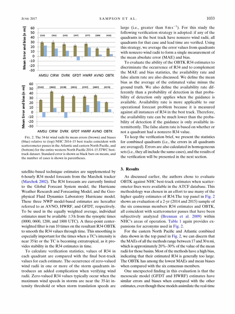
higher quality estimates of R34.The top panel in Fig. 2

shows an evaluation of a 2-yr (2014 and 2015) sample of

the six consensus members R34 estimates and OBTK,

all coincident with scatterometer passes that have been

subjectively analyzed (Brennan et al. 2009) within

NHC’s areas of operation. Table 1 again provides ex-

pansions for acronyms used in Fig. 2.

For the eastern North Pacific and Atlantic combined

data shown in the top panel in Fig. 2, we can discern that

theMAEs of all themethods range between 17 and 30nmi,

which is approximately 20%–30%of the value of themean

radii for those basins.Most of themethods have a high bias,

indicating that their estimated R34 is generally too large.

The OBTK has among the lowest MAEs and mean biases

when compared with the six consensus members.

One unexpected finding in this evaluation is that the

mesoscale model (GFDT and HWRF) estimates have

similar errors and biases when compared with the other

estimates, even though thesemodels assimilate the real-time

FIG. 2. The 34-kt wind radii fix mean errors (brown) and biases

(blue) relative to (top) NHC 2014–15 best tracks coincident with

scatterometer passes in the Atlantic and eastern North Pacific, and

(bottom) for the entire western North Pacific 2014–15 JTWC best-

track dataset. Standard error is shown as black bars on means, and

the number of cases is shown in parentheses.

JUNE 2017 SAMPSON ET AL . 1033

NHC wind radii estimates. The CIRW and AVNO both

assimilate scatterometer winds, and AVNO also ap-

pears to have the lowest MAE and bias compared with

the best-track estimates coincident with scatterometer

passes (Fig. 2, top). The interplay between best-track

R34 uncertainty, interdependence of the estimates, and

ground truth coincident with scatterometer passes

presents issues that will not be addressed in this study.

The bottompanel in Fig. 2 shows the performance of the

sameR34 estimates and the equally weightedmean for the

newly created 2014–15 western North Pacific best tracks.

The MAE values in the estimates are higher than in the

NHC dataset, ranging from approximately 21 to 42nmi,

but they still represent approximately 20%–30% of the

mean radius for the dataset in that basin (see Table 2). The

biases range from 212 to 21nmi and are not consistent

with the biases in theNHCdata. ThewesternNorthPacific

dataset is not limited to best-track data with coincident

scatterometer passes, and in this sample the AVNO esti-

mates are now on par with the other estimates. TheOBTK

has the lowest MAE and a small positive bias comparable

to its bias in theNHC dataset. An inspection of theOBTK

values for both datasets indicates that these mean R34

estimates generally vary slowly with time compared with

the individual estimates, which is a desirable feature for

maintaining consistency in operational analysis and fore-

casting. The standard deviation of the OBTK errors

(14nmi) provides one measure of R34 uncertainty.

Another benefit of the OBTK is that it is designed to

have nearly 100% availability (Fig. 3). An availability

rate of less than 100% is expected for each of the in-

dividual estimates and is somewhat problematic for

forecasters who need guidance for all their official R34

estimates. The AMSU-based R34 estimates are rea-

sonably accurate (see Fig. 2), but their availability rate

is limited to approximately 35% of the time as a result

of the geometry of polar satellite orbit overpasses

and a 1400-km effective swath. The other individual

estimate availability rates are between 70% and 90%,

and the OBTK availability is nearly 98% for this

dataset.

The number of cases where observed radii do not exist

(857) is about 20% as large as the number of cases where

R34 exists. The OBTK false alarm rate is 50% (423 out

of 857 cases). In operational forecasting, a high false

alarm rate is not necessarily a liability since the opera-

tional forecast intensity (35 kt or greater for our sample)

determines whether or not the forecaster creates real-

time R34 estimates. The authors also consider a high

false alarm rate to be a benefit since it could also provide

advanced guidance of TC structure when the TC reaches

35 kt—noting that the uncertainty of the intensity anal-

ysis estimates is on the order of 10 kt (Landsea and

Franklin 2013; Torn and Snyder 2012).

We have made no effort to correct biases in or un-

evenly weight the individual estimates in the OBTK

since it is our opinion (and others, e.g., Kharin and

Zwiers 2002; Weigel et al. 2010; DelSole et al. 2013)

that assigning weights to the individual estimates is

difficult, especially when the accuracy of the individ-

ual estimates is changing with time (e.g., the NWP

model estimates should improve as the NWP models

improve). Also, an inspection of the entire dataset

indicates that the OBTK estimates are more consis-

tent with time when more of the individual estimates

are available. When the number of the individual es-

timates is low (e.g., at the beginning or near the end

of a TC life cycle when there may only be between one

and three estimates available), the OBTK R34 esti-

mates can change rapidly with time. This is an un-

desirable feature for operational forecasting, so

additional R34 estimates (e.g., from other NWP

TABLE 2. The 2014 and 2015 best-track climatological mean 34-kt wind radii, mean error, and bias in the real-time subjective estimates

from the forecasters.

Basin No. of cases

Best-track mean

R34 (nmi)

Real-time estimate

MAE (nmi)

Real-time estimate

bias (nmi)

Atlantic 974 95 6 22

Eastern North Pacific 3070 82 3 0

Western North Pacific 3707 134 30 227

FIG. 3. Wind radii estimate availability based on 4251 best-track radius

estimates for the JTWC western North Pacific 2014–15 seasons.

1034 WEATHER AND FORECAST ING VOLUME 32

models and from other satellite-databased algorithms)

would likely improve the operational utility of the

OBTK. Also, increasing the number of independent

estimates (e.g., estimates from different satellite

platforms) should also improve OBTK performance,

similar to findings in efforts to improve TC track and

intensity forecast guidance (see Goerss et al. 2004;

Sampson et al. 2008).

4. Conclusions and recommendations

In this paper we have evaluated six individual esti-

mates of R34 against NHC best tracks (described in

appendix A) coincident with scatterometer passes from

2014 and 2015 and found that the estimates had errors

that ranged between 17 and 30 nmi, and had biases that

ranged between 28 and 23nmi. We then formed an

equally weighted mean of these estimates (OBTK), and

found its performance to be among the best in terms of

both error and bias when compared with the NHC best-

track estimates.

We then applied our algorithm to the western North

Pacific 2014 and 2015 seasons to create higher quality

R34 estimates for use in reanalyzing the JTWC R34

estimates. In appendix B we performed a double-blind

study to create a subjective best track of R34 on one

eastern North Pacific TC (Blanca from the 2015 season)

and found that our independent R34 estimates com-

pared favorably with those of the NHC. We then

created a 2-yr subjective reanalysis (best track) of R34

for the western North Pacific.We found that the average

R34 value for our western North Pacific best track is

134nmi, which is much higher than the average of real-

time western North Pacific estimates (103 nmi). For

comparison, the average R34 is 95 nmi in the Atlantic

best tracks and 82nmi in the eastern North Pacific best

tracks for the same years. The OBTK mean error rela-

tive to some of the highest quality NHC R34 estimates

(those coincident with scatterometer passes) is 17 n mi,

and the standard deviation (a measure of uncertainty)

is 14 nmi. Uncertainty estimates for best-track radii

without coincident scatterometer passes are expected

to be higher.

Now that we have a way of producing higher quality

estimates of R34 in the western North Pacific, we can

apply our methodology to other years and other ba-

sins to create a higher quality best-track R34 record

for use in climatology studies (e.g., Wu et al. 2015).

This higher quality record can also be used to (re)develop

guidance such as the wind radii climatology and persis-

tence model (Knaff et al. 2007), wind radii consensus aids

(see Sampson and Knaff 2015), and consensus-based

error estimates similar to those created for intensity

in Goerss and Sampson (2014). These guidance improve-

ments would then be available to operational forecasters

and have implications for end-user products such as

those discussed in the introduction. The OBTK could

possibly be improved by the addition of more quality

wind radii guidance. Some potential methods include

the IR-based method discussed in Dolling et al. (2016),

Global Navigation Satellite System reflectometry

methods (Ruf et al. 2016) and L-band microwave-based

methods discussed in Reul et al. (2016) and Meissner

et al. (2014). These methods will be investigated as

OBTK members in the near future.

Finally, there is hope of improving the estimates of the

50- and 64-kt wind radii. Not only is there evidence of

dependence of these radii on the 34-kt wind radii (see

Knaff et al. 2016), but there are already several indepen-

dent satellite-based estimates of these radii that could be

used to develop this capability.

Acknowledgments. The authors would like to ac-

knowledge the staff at NHC and JTWC, the NOAA

GOES and GOES-R program offices for support of

TC structure studies, and the important behind-the-

scenes efforts of Ann Schrader and Mike Frost.

Careful reading of reviewers and managers from

several agencies is also acknowledged. Specifically,

we thank Chris Landsea, Ed Rappaport, and Todd

Kimberlain of NHC for comments on previous versions

of this manuscript. This publication was graciously

funded by the Office of Naval Research, Program

Elements 0602435N. The views, opinions, and findings

contained in this report are those of the authors and

should not be construed as an official National Oce-

anic and Atmospheric Administration or U.S. gov-

ernment position, policy, or decision.

APPENDIX A

NHC 34-kt Wind Radii Postanalysis

At the National Hurricane Center (NHC), 34-kt wind

radii are reanalyzed as part of the poststorm ‘‘best

track’’ analysis of the tropical cyclone (and its post-

tropical stage, if applicable). These analyses are valid at

0000, 0600, 1200, and 1800 UTC, and this reanalysis also

includes the location of the TC center, its intensity, and

50- and 64-kt wind radii.

Available data for postanalysis in NHC’s AOR include

in situ ship, buoy, and land observations; flight-level

winds and stepped-frequency microwave radiometer

surface wind speed measurements from aircraft

reconnaissance; dropwindsondes from aircraft; scat-

terometer winds; and estimates of wind radii from

JUNE 2017 SAMPSON ET AL . 1035

microwave sounders such as AMSU. The amount of

data available for each TC and at various times within

the same TC’s life cycle varies widely. For example,

aircraft reconnaissance data are only available in about

30% of Atlantic TCs (mostly in the western part of

the basin), and only rarely in TCs in the eastern North

Pacific basin (typically when hurricanes threaten the

coast of Mexico). Even when aircraft data are available,

the point data available along the aircraft flight path

typically sample only about 2% of the TC’s wind field

in a full ‘‘alpha’’ pattern through the cyclone. Scatter-

ometers can provide better spatial coverage of winds,

but passes are at most available only twice a day from

low-Earth satellites in polar orbit at the low and mid-

latitudes where most TCs are found. There are also

gaps between scatterometer data swaths, especially in

the tropics, that can result in sampling only part of the

TC wind field or total ‘‘misses’’ for multiple passes in a

row. In situ surface observations are even more spo-

radic and are, typically, found close to major land-

masses and islands, particularly in the western

Atlantic basin. Most of the eastern North Pacific basin

is completely devoid of in situ wind data apart from in-

frequent aircraft flights, as mentioned above, or occa-

sional ship data.

The starting point for the reanalysis is the opera-

tional 34-kt wind radii that were made in real time by

the duty hurricane specialist. Given that these real-

time estimates are made under operational time con-

straints, and that most remotely sensed data have some

temporal latency that results in a 1–3-h delay in the

receipt of the data, the postanalysis process provides

an opportunity to revisit the 34-kt wind radii in a

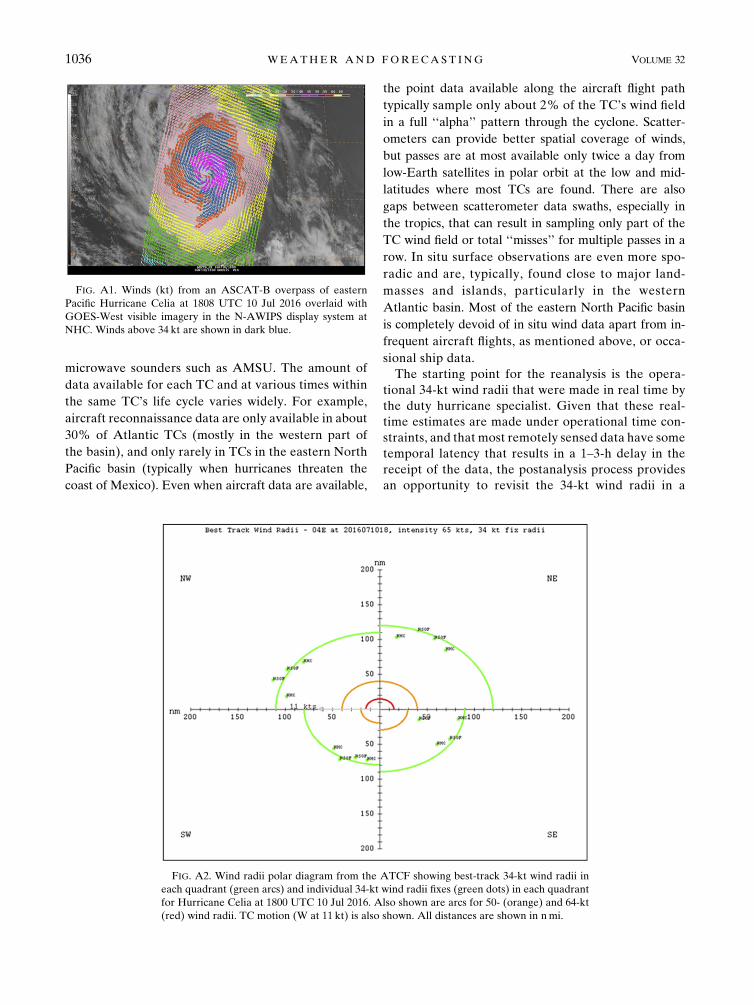
FIG. A2. Wind radii polar diagram from the ATCF showing best-track 34-kt wind radii in

each quadrant (green arcs) and individual 34-kt wind radii fixes (green dots) in each quadrant

for Hurricane Celia at 1800 UTC 10 Jul 2016. Also shown are arcs for 50- (orange) and 64-kt

(red) wind radii. TC motion (W at 11 kt) is also shown. All distances are shown in nmi.

FIG. A1. Winds (kt) from an ASCAT-B overpass of eastern

Pacific Hurricane Celia at 1808 UTC 10 Jul 2016 overlaid with

GOES-West visible imagery in the N-AWIPS display system at

NHC. Winds above 34 kt are shown in dark blue.

1036 WEATHER AND FORECAST ING VOLUME 32

more holistic manner and with the benefit of having

all the data available for the analysis. Given the un-

certainty and often the lack of data involved in the

analysis process, NHC currently rounds 34-kt wind

radii in each quadrant to the nearest 10 nmi and

tries to show bulk trends in the wind field that can

be captured by the temporal resolution of a 6-h

best track.

During the reanalysis process, all available data are

used, with the most weight given to direct wind mea-

surements from aircraft, scatterometry, and surface

data. When there are large spatial gaps between the

available data, such as in open-ocean storms, the anal-

ysis is typically anchored on available data, such as

scatterometer passes, and the analysis at times between

those observations is smoothed to fit the available data

at the beginning and end of the period, taking into ac-

count intervening changes in the intensity, motion, and

structure of the TC.

These data are viewed in a variety of platforms.Aircraft

data, surface observations, and scatterometer data are

available in the N-AWIPS software system, which allows

the analyst to overlay the data together with geostationary

satellite imagery and measure the wind radii directly

(Fig. A1). Wind radii ‘‘fixes’’ are also entered into the

ATCF database and are available for viewing both in

text and graphical formats (Fig. A2).

APPENDIX B

JTWC 34-kt Wind Radii Postanalysis

JTWC real-time estimates of R34 in the western

North Pacific are largely based on timely scatterometer

passes, multiplatform satellite wind analyses, analysis of

microwave and infrared imagery patterns, and occa-

sional ship and station observations. Although routine

aircraft reconnaissance operations ended in 1987, occa-

sionally aircraft data are available to forecasters for TCs

approaching Taiwan. When noted observations are

unavailable in real time, the JTWC R34 estimates are

generally persistence from prior estimates.

For the 2014–15 postseason R34 analyses, storm-

following imagery (scatterometer winds, visible and IR

imagery, and microwave imagery) was obtained from

the Fleet Numerical Meteorology Center and the Na-

val Research Laboratory Tropical Cyclone Page web-

site (Fig. B1). NWP 6-h forecasts of R34 from the

Global Forecast System andHurricaneWeatherResearch

Forecast System were obtained from the ATCF archive,

as were AMSU-based and multiplatform-based wind

radii estimates. Geophysical Fluid Dynamics Laboratory

NWP model wind radii were obtained from reruns for

both the 2014 and 2015 seasons. Dvorak wind radii

estimates were computed postseason using the Naval

FIG. B1. Examples of the imagery used to determine 1200 UTC 6 Sep R34 estimates for

Chan-Hom, the ninth TC of the JTWC western North Pacific 2015 season. (top left) Scatter-

ometer imagery at 1141 UTC 6 Sep, (top right) 91-GHz imagery at 0949 UTC 6 Sep, (bottom

left) 89-Ghz imagery at 1140 UTC 6 Sep, and (bottom right) enhanced infrared imagery at

1132 UTC 6 Sep. R34 postseason estimates are shown for comparison.

JUNE 2017 SAMPSON ET AL . 1037

Research Laboratory Tropical Cyclone Page imagery

and the JTWC Dvorak estimates.

The position and intensity best tracks, already ana-

lyzed postseason, were taken from the ATCF archive

and reviewed from start to finish. Then, noted imagery

was overlaid onto JTWC real-time R34 estimates.

JTWC real-time R34 estimates were compared with the

OBTK described in the body of this paper and, when

scatterometer imagery was unavailable, the members of

OBTK were used as a baseline or first guess. Temporal

FIG. B3. (left) NHC 34-kt wind radii estimates (black line) through time for the north-

eastern quadrant in Blanca (ep022015) with scatterometer fixes (purple) and AMSU es-

timates (salmon). (right) NRL reanalysis of the same quadrant (solid black line) completed

using objective estimates (multicolored dots) and an equally weighted average of the

objective estimates (dashed line), scatterometer data, and other resources. In both plots,

the observed intensity (kt) at 12-h intervals is indicated along the top of the plot in

light green.

FIG. B2. Wind radii vs time plot for the northeastern quadrant of Chan-Hom. Yellow dots

indicate real-time JTWC estimates, other dots indicate objective estimates, the dashed black

line indicates the equally weighted average, and the red line indicates the postseason analysis.

1038 WEATHER AND FORECAST ING VOLUME 32

continuity in the estimates was also considered (see

Fig. B2). As in theNHCprocedure, R34 was determined

for all intensities of 35 kt or greater. R34 was specified in

increments of 15 nmi in order to minimize small and

short-term fluctuations. For each R34 estimate, justifi-

cations were recorded in logs and saved in the ATCF

archive.

Since the R34 postseason analysis at JTWC is a new

effort, we were unsure of the quality of our reanalyzed

R34 values, particularly given the sparsity of quality

observational data. To validate the methods and pro-

cesses, we ran a double-blind experiment using a fairly

well-behaved tropical cyclone in the eastern North

Pacific (Fig. B3). Using only the fixes and imagery

available in the ATCF (no aircraft data and no estimates

from NHC), we produced our own independent estimates

of R34 for this TC. The results in Fig. B3, though anec-

dotal, show that our methodology provided estimates

similar in size to those of the NHC postseason analysis.

Differences do exist, as they do between the objective

estimates and NHC best tracks. Most of the large differ-

ences are within the 20% (or 30nmi) range. The largest

differences are in the R34 estimates both at the beginning

and end of the TC life cycle.

REFERENCES

Bates, J. M., and C. W. J. Granger, 1969: The combination of

forecasts. Oper. Res., 20, 451–468, doi:10.1057/jors.1969.103.

Bender, M. A., M. J. Morin, K. Emanuel, J. A. Knaff, C. Sampson,

I.Ginis, andB. Thomas, 2016: Impact of storm structure and the

environmental conditions in the rapid intensification of Hurri-

canes Katrina and Patricia. 32nd Conf. on Hurricanes and

TropicalMeteorology, San Juan, PR,Amer.Meteor. Soc., 6D.2.

[Available online at https://ams.confex.com/ams/32Hurr/

webprogram/Paper293687.html.]

Bentamy, A., D. Croize-Fillon, and C. Perigaud, 2008: Characteriza-

tion of ASCAT measurements based on buoy and QuikSCAT

wind vector observations. Ocean Sci., 4, 265–274, doi:10.5194/

os-4-265-2008.

Boukabara, S. A., and Coauthors, 2011: MiRS: An all-weather

1DVAR satellite data assimilation and retrieval system. IEEE

Trans. Geosci. Remote Sens., 49, 3249–3272, doi:10.1109/

TGRS.2011.2158438.

Brennan, M. J., C. C. Hennon, and R. D. Knabb, 2009: The oper-

ational use of QuikSCAT ocean surface vector winds at the

National Hurricane Center. Wea. Forecasting, 24, 621–645,

doi:10.1175/2008WAF2222188.1.

Cangialosi, J. P., and C. W. Landsea, 2016: An examination of

model and official National Hurricane Center tropical cyclone

size forecasts. Wea. Forecasting, 31, 1293–1300, doi:10.1175/

WAF-D-15-0158.1.

Chou, K.-H., C.-C. Wu, and S.-Z. Lin, 2013: Assessment of the

ASCAT wind error characteristics by global dropwindsonde

observations. J. Geophys. Res., 118, 9011–9021, doi:10.1002/

jgrd.50724.

DelSole, T., X. Yang, and M. K. Tippett, 2013: Is unequal

weighting significantly better than equal weighting for

multi-model forecasting? Quart. J. Roy. Meteor. Soc., 139,

176–183, doi:10.1002/qj.1961.

DeMaria, M., and Coauthors, 2013a: Improvements to the

operational tropical cyclone wind speed probability model.Wea.

Forecasting, 28, 586–602, doi:10.1175/WAF-D-12-00116.1.

——, A. Schumacher, J. Dostalek, S. Longmore, L. Zhao, and

L. Ma, 2013b: S-NPP microwave sounder-based TC prod-

ucts algorithm theoretical basis document. NOAA/NESDIS,

18 pp. [Available online at http://www1.ncdc.noaa.gov/pub/

data/metadata/documents/C00937_Algorithm_Theoretical_Basis_

Document_NTCP_v1.1.docx.]

——, C. R. Sampson, J. A. Knaff, and K. D. Musgrave, 2014: Is

tropical cyclone intensity guidance improving? Bull. Amer.

Meteor. Soc., 95, 387–398, doi:10.1175/BAMS-D-12-00240.1.

Demuth, J. L.,M.DeMaria, J.A.Knaff, andT.H.VonderHaar, 2004:

Evaluation of Advanced Microwave Sounder Unit (AMSU)

tropical cyclone intensity and size estimation algorithm. J. Appl.

Meteor., 43, 282–296, doi:10.1175/1520-0450(2004)043,0282:

EOAMSU.2.0.CO;2.

——, ——, and ——, 2006: Improvement of Advanced Microwave

Sounding Unit tropical cyclone intensity and size estimation

algorithms. J. App. Meteor. Climatol., 45, 1573–1581,

doi:10.1175/JAM2429.1.

Dolling, K., E. A. Ritchie, and J. S. Tyo, 2016: The use of the

deviation angle variance technique on geostationary

satellite imagery to estimate tropical cyclone size parame-

ters. Wea. Forecasting, 31, 1625–1642, doi:10.1175/

WAF-D-16-0056.1.

Dostalek, J., G. Chirokova, J. Knaff, S. Longmore, R. T. DeMaria,

A. B. Schumacher, and C. Sampson, 2016: Recent and future

updates to the operational, satellite-based tropical cyclone

products produced at the Cooperative Institute for Research

in the Atmosphere. 32nd Conf. on Hurricanes and Tropical

Meteorology, San Juan, PR, Amer. Meteor. Soc., 11C.7.

[Available online at https://ams.confex.com/ams/32Hurr/

webprogram/Paper293020.html.]

Dvorak, V. F., 1984: Tropical cyclone intensity analysis using

satellite data. NOAA Tech. Rep. NESDIS 11, 45 pp. [Avail-

able online at ftp://satepsanone.nesdis.noaa.gov/Publications/

Tropical/Dvorak_1984.pdf.]

Elliott, G., and M. Yamaguchi, 2014: Motion—Recent advances.

Summary Rep. on Eighth Int. Workshop on Tropical Cy-

clones (IWTC-8), WMO, 44 pp. [Available online at http://

www.wmo.int/pages/prog/arep/wwrp/new/documents/Topic1_

AdvancesinForecastingMotion.pdf.]

Goerss, J. S., and C. R. Sampson, 2014: Prediction of consensus

tropical cyclone intensity forecast error.Wea. Forecasting, 29,

750–762, doi:10.1175/WAF-D-13-00058.1.

——, ——, and J. Gross, 2004: A history of western North Pa-

cific tropical cyclone track forecast skill. Wea. Forecast-

ing, 19, 633–638, doi:10.1175/1520-0434(2004)019,0633:

AHOWNP.2.0.CO;2.

Goldberg, M. D., D. S. Crosby, and L. Zhou, 2001: The limb

adjustment of AMSU-A observations: Methodology and

validation. J. Appl. Meteor., 40, 70–83, doi:10.1175/

1520-0450(2001)040,0070:TLAOAA.2.0.CO;2.

Harr, P.A., andN.Kitabatake, 2015: Structure and structure change.

Eighth Int. Workshop on Tropical Cyclones, Jeju Island, South

Korea, WMO, T4. [Available online at http://www.wmo.int/

pages/prog/arep/wwrp/new/documents/Topic4.pdf.]

Kharin, V. V., and F. W. Zwiers, 2002: Climate predictions with

multimodel ensembles. J. Climate, 15, 793–799, doi:10.1175/

1520-0442(2002)015,0793:CPWME.2.0.CO;2.

JUNE 2017 SAMPSON ET AL . 1039

Knaff, J. A., and B. A. Harper, 2010: Tropical cyclone surface wind

structure and wind-pressure relationships. Seventh Int. Workshop

on Tropical Cyclones, La Reunion, France, WMO, KN1.

[Available online at https://www.wmo.int/pages/prog/arep/

wwrp/tmr/otherfileformats/documents/KN1.pdf.]

——, andC. R. Sampson, 2015: After a decade areAtlantic tropical

cyclone gale force wind radii forecasts now skillful? Wea.

Forecasting, 30, 702–709, doi:10.1175/WAF-D-14-00149.1.

——, C. Guard, J. Kossin, T. Marchok, C. Sampson, T. Smith,

and N. Surgi, 2006: Operational guidance and skill in fore-

casting structure change. Sixth Int. Workshop on Tropical

Cyclones, San Juan, Costa Rica, WMO, 160–184. [Available

online at http://severe.worldweather.org/iwtc/document/

Topic_1_5_John_Knaff.pdf.]

——, C. R. Sampson, M. DeMaria, T. P. Marchok, J. M. Gross, and

C. J. McAdie, 2007: Statistical tropical cyclone wind radii pre-

diction using climatology and persistence.Wea. Forecasting, 22,

781–791, doi:10.1175/WAF1026.1.

——, M. DeMaria, D. A. Molenar, C. R. Sampson, and M. G.

Seybold, 2011: An automated, objective, multisatellite plat-

form tropical cyclone surface wind analysis. J. Appl. Meteor.

Climatol., 50, 2149–2166, doi:10.1175/2011JAMC2673.1.

——, C. J. Slocum, K. D. Musgrave, C. R. Sampson, and B. Strahl,

2016: Using routinely available information to estimate trop-

ical cyclone wind structure. Mon. Wea. Rev., 144, 1233–1247,

doi:10.1175/MWR-D-15-0267.1.

Kossin, J. P., J.A.Knaff,H. I. Berger,D.C.Herndon, T.A.Cram,C. S.

Velden, R. J. Murnane, and J. D. Hawkins, 2007: Estimating

hurricanewind structure in the absence of aircraft reconnaissance.

Wea. Forecasting, 22, 89–101, doi:10.1175/WAF985.1.

Kunii, M., 2015: Assimilation of tropical cyclone track and wind

radius data with an ensemble Kalman filter.Wea. Forecasting,

30, 1050–1063, doi:10.1175/WAF-D-14-00088.1.

Kurihara, Y., M. A. Bender, and R. J. Ross, 1993: An initialization

scheme of hurricane models by vortex specification.Mon. Wea.

Rev., 121, 2030–2045, doi:10.1175/1520-0493(1993)121,2030:

AISOHM.2.0.CO;2.

Landsea, C.W., and J. L. Franklin, 2013: Atlantic hurricane database

uncertainty and presentation of a new database format. Mon.

Wea. Rev., 141, 3576–3592, doi:10.1175/MWR-D-12-00254.1.

Magnan, S.G., 1998:Calculating tropical cyclone critical wind radii and

storm size using NSCAT winds. M.S. thesis, Naval Postgraduate

School, 55 pp. [Available online at http://calhoun.nps.edu/

bitstream/handle/10945/8044/calculatingtropi00magn.pdf?

sequence51&isAllowed5y.]

Marchok, T. P., 2002: How the NCEP tropical cyclone tracker works.

Preprints, 25th Conf. on Hurricanes and Tropical Meteorology,

San Diego, CA, Amer. Meteor. Soc., P1.13. [Available online at

https://ams.confex.com/ams/pdfpapers/37628.pdf.]

——, M. Morin, and M. Bender, 2012: Evaluation of a GFDL hur-

ricane model ensemble forecast system. 30th Conf. on Hurri-

canes and Tropical Meteorology, Ponte Verde, FL, Amer.

Meteor. Soc., 13A.3. [Available online at https://ams.confex.

com/ams/30Hurricane/webprogram/Paper206200.html.]

Meissner, T., F. J.Wentz, andL. Ricciardulli, 2014: The emission and

scattering of L-band microwave radiation from rough ocean

surfaces and wind speed measurements from the Aquarius

sensor. J. Geophys. Res. Oceans, 119, 6499–6522, doi:10.1002/

2014JC009837.

Mueller, K. J., M. DeMaria, J. A. Knaff, J. P. Kossin, and T. H.

Vonder Haar, 2006: Objective estimation of tropical cyclone

wind structure from infrared satellite data. Wea. Forecasting,

21, 990–1005, doi:10.1175/WAF955.1.

NHC, 2016, Introduction to storm surge. National Hurricane

Center/Storm Surge Unit, 5 pp. [Available online at http://

www.nhc.noaa.gov/surge/surge_intro.pdf.]

Powell, M. D., and T. A. Reinhold, 2007: Tropical cyclone de-

structive potential by integrated kinetic energy. Bull. Amer.

Meteor. Soc., 88, 513–526, doi:10.1175/BAMS-88-4-513.

Quiring, S., A. Schumacher, and S. Guikema, 2014: Incorporating

hurricane forecast uncertainty into decision support applica-

tions. Bull. Amer. Meteor. Soc., 95, 47–58, doi:10.1175/

BAMS-D-12-00012.1.

Reul, N., B. Chapron, E. Zabolotskikh, C. Donlon, Y. Quilfen,

S. Guimbard, and J. F. Piolle, 2016: A revised L-band radio-

brightness sensitivity to extreme winds under tropical cyclone:

The 5 year SMOS-storm database. Remote Sens. Environ.,

180, 274–291, doi:10.1016/j.rse.2016.03.011.Ruf, C., and Coauthors, 2016: New ocean winds satellite mission to

probe hurricanes and tropical convection.Bull. Amer. Meteor.

Soc., 97, 385–395, doi:10.1175/BAMS-D-14-00218.1.

Sampson, C. R., andA. J. Schrader, 2000: TheAutomated Tropical

Cyclone Forecasting System (version 3.2).Bull. Amer.Meteor.

Soc., 81, 1231–1240, doi:10.1175/1520-0477(2000)081,1231:

TATCFS.2.3.CO;2.

——, and J. Knaff, 2015: A consensus forecast for tropical cyclone

gale wind radii. Wea. Forecasting, 30, 1397–1403, doi:10.1175/

WAF-D-15-0009.1.

——, J. L. Franklin, J. A. Knaff, and M. DeMaria, 2008: Experi-

ments with a simple tropical cyclone intensity consensus.Wea.

Forecasting, 23, 304–312, doi:10.1175/2007WAF2007028.1.

——, P. A. Wittmann, and H. L. Tolman, 2010: Consistent tropical

cyclone wind and wave forecasts for the U.S. Navy. Wea.

Forecasting, 25, 1293–1306, doi:10.1175/2010WAF2222376.1.

——, and Coauthors, 2012: Objective guidance for use in setting

tropical cyclone conditions of readiness.Wea. Forecasting, 27,1052–1060, doi:10.1175/WAF-D-12-00008.1.

Student, 1908: The probable error of a mean. Biometrika. 6, 1–25,

doi:10.2307/2331554.

Tallapragada,V., andCoauthors, 2015:HurricaneWeatherResearch

and Forecasting (HWRF) Model: 2015 scientific documen-

tation, August 2015 – HWRF v3.7a. NCAR Developmen-

tal Testbed Center, Boulder, CO, 123 pp. [Available online

at http://www.dtcenter.org/HurrWRF/users/docs/scientific_

documents/HWRF_v3.7a_SD.pdf.]

Torn, R., and C. Snyder, 2012: Uncertainty of tropical cyclone best-

track information.Wea. Forecasting, 27, 715–729, doi:10.1175/

WAF-D-11-00085.1.

Weigel, A. P., R. Knutti, M. A. Liniger, and C. Appenzeller, 2010:

Risks of model weighting in multimodel climate projections.

J. Climate, 23, 4175–4191, doi:10.1175/2010JCLI3594.1.Wu, C.-C., G.-Y. Lien, J.-H. Chen, and F. Zhang, 2010: Assimila-

tion of tropical cyclone track and structure based on the en-

semble Kalman filter (EnKF). J. Atmos. Sci., 67, 3806–3822,

doi:10.1175/2010JAS3444.1.

Wu, L., W. Tian, Q. Liu, J. Cao, and J. A. Knaff, 2015: Implications

of the observed relationship between tropical cyclone size and

intensity over the western North Pacific. J. Climate, 28, 9501–

9506, doi:10.1175/JCLI-D-15-0628.1.

1040 WEATHER AND FORECAST ING VOLUME 32