trophic structure and dynamical complexity in simple ecological models

e c o l o g i c a l c o m p l e x i t y 4 ( 2 0 0 7 ) 2 1 2 – 2 2 2

Trophic structure and dynamical complexity in simpleecological models

Vikas Rai d, Madhur Anand a,b,*, Ranjit Kumar Upadhyay c

aDepartment of Biology, Laurentian University, Ramsey Lake Road, Sudbury, Ontario, Canada P3E 2C6bDepartment of Environmental Biology, University of Guelph, Guelph, Ontario, Canada N1G 2W1cDepartment of Applied Mathematics, Indian School of Mines University, Dhanbad, Jharkhand 826004, IndiadDepartment of Applied Mathematics, HMR Institute of Technology and Management, GT Karnal Road, Delhi 110 036, India

a r t i c l e i n f o

Article history:

Received 2 April 2007

Received in revised form

27 June 2007

Accepted 27 June 2007

Published on line 13 August 2007

Keywords:

Predator–prey interaction

Generalist and specialist predators

Competition

Population cycles

Food web

Deterministic chaos

Robust chaos

Short-term recurrent chaos

a b s t r a c t

We study the dynamical complexity of five non-linear deterministic predator–prey model

systems. These simple systems were selected to represent a diversity of trophic structures

and ecological interactions in the real world while still preserving reasonable tractability.

We find that these systems can dramatically change attractor types, and the switching

among different attractors is dependent on system parameters. While dynamical complex-

ity depends on the nature (e.g., inter-specific competition versus predation) and degree (e.g.,

number of interacting components) of trophic structure present in the system, these

systems all evolve principally on intrinsically noisy limit cycles. Our results support the

common observation of cycling and rare observation of chaos in natural populations. Our

study also allows us to speculate on the functional role of specialist versus generalist

predators in food web modeling.

# 2007 Elsevier B.V. All rights reserved.

avai lable at www.sc iencedi rec t .com

journal homepage: ht tp : / /www.e lsev ier .com/ locate /ecocom

1. Introduction

Dynamical complexity refers to the variety of behaviors that

systems can exhibit over time. It can be studied through

construction of simple models, and then examination of

patterns in temporal evolution in response to changes in

model parameters. As such one can attempt to estimate the

likelihood of observing predictable (e.g., simple equilibrium,

cycles) versus unpredictable (chaotic) dynamics in phase

space and determine what causes abrupt changes between

these two types of behavior. The more likely the occurrence

of unpredictability and abrupt changes in system dynamics,

* Corresponding author at: Department of Environmental Biology, UniTel.: +1 519 824 4120; fax: +1 519 837 0442.

E-mail address: [email protected] (M. Anand).

1476-945X/$ – see front matter # 2007 Elsevier B.V. All rights reservedoi:10.1016/j.ecocom.2007.06.010

the more dynamically complex a system is understood

to be.

Typically, dynamical complexity can be studied by finding

the critical parameter values which cause changes in attractor

types. Take the classic single population dynamic model

studied by May (1975, 1976) and May and Oster (1976). In this

model, there is only one parameter to be varied, namely r, the

intrinsic growth rate. For some range of r values, dynamics

reaches a single equilibrium. For another range, the attractor

is cyclical. Once it reaches a critical point (r = 3.5), chaos is

observed. Because there is no interruption in the display of

chaotic behavior as r is increased further, we call this type of

versity of Guelph, Guelph, Ontario, Canada N1G 2W1.

d.

mailto:[email protected]

http://dx.doi.org/10.1016/j.ecocom.2007.06.010

e c o l o g i c a l c o m p l e x i t y 4 ( 2 0 0 7 ) 2 1 2 – 2 2 2 213

chaotic dynamics ‘‘robust’’. This behavior illustrates a very

important property: the fact that an extremely simple model

(e.g., a single population model) can display dynamical

complexity. However, as we shall see, the dynamical complex-

ity of this model is actually relatively low, when compared to

more structurally complex ecological models. This is because

it has a critical parameter value that clearly divides the phase

space into different attractor types (fixed points, stable limit

cycles, and chaos).

In this paper, we investigate the dynamical complexity of

predator–prey models. The simplest predator–prey model is the

Lotka–Volterra model (Lotka, 1920; Volterra, 1931). Because of

the existence of two interacting populations, one can argue that

this model is structurally more complex than the one studied by

May (1976). However, perhaps surprisingly, it does not display

greater dynamical complexity. In fact, one can argue that it

displays less dynamical complexity than the single population

dynamic model because there is no chaotic behavior. Several

studies, most of which build upon the work of Lotka, Volterra

and May, have however now reported robust deterministic

chaos in an appreciable range of a single critical parameter of

model predator–prey systems with three or more interacting

populations (Gilpin, 1979; Schaffer, 1985; Hastings and Powell,

1991; Rai and Sreenivasan, 1993; Rinaldi and Muratori, 1993;

Rinaldi et al., 1993; Vandermeer, 1993; Klebanoff and Hastings,

1994; King et al., 1996, 2004; Upadhyay and Rai, 1997; Edwards

and Bees, 2001; Vandermeer et al., 2001; Aziz-Alaoui, 2002). Very

few studies on predator-prey systems attempt to examine if the

chaotic dynamics is robust with respect to changes in system

parameters in a two-dimensional (2D) space. The study of

Samardzija and Greller (1988) is an exception. These authors

found that their model could exhibit chaotic dynamics in

surprising regions of parameter space due to a ‘‘fractal torus

structure’’, hence introducing the term ‘‘explosive chaos’’.

While their model included only three interacting populations,

they noted that the use of two predators and one prey was

distinctly different from previous models which included one

predator and two prey (e.g., Arneodo et al., 1980; Gilpin, 1979;

Schaffer, 1985), because these previous models all showed

robust chaos. Thus, we should expect that the structure of

models (not just the number of interacting populations) should

also affect dynamical complexity.

Generally speaking, we can expect that when there are

more parameters to be investigated, the dynamical complex-

ity of a model should increase. Indeed, while performing

simulation studies of a new class of predator–prey models,

Upadhyay et al. (1998) discovered that the presence of chaotic

dynamics is not robust to changes in paired system para-

meters. Namely, there were no large smooth regions in

parameter space with which one could identify a chaotic

phase. Similarly, Turchin and Ellner (2000) discovered an

interesting variety of chaos which they termed short-term

recurrent chaos (called strc hereafter). In this type of dynamical

complexity, chaotic behavior is interrupted by other kinds of

dynamics at irregular and unpredictable intervals. This

phenomenon also occurs in several other predator–prey

models (Upadhyay and Rai, 2001; Rai, 2004; Rai and Anand,

2004; Rai and Upadhyay, 2004).

In this paper, we examine a suite of predator–prey models

to attempt to shed light on when we should expect to see strc

versus robust chaos. We hypothesize that the reason why

chaos is rarely observed in natural populations might lie with

the structure of ecological systems (e.g., one versus two

predators) and the nature of ecological interactions (e.g.,

competition, mutualism and predation). We use some

published models, but also create new models by manipulat-

ing the trophic structure in simple coupled oscillators. As

such, we attempt to explore the diversity of interaction effects

on simple ecological systems.

2. Model systems

There are three ways to generate chaos in a mathematical

model: (1) by coupling two non-linear oscillators (Vandermeer,

1993, 2004; Rai, 2004), (2) by incorporating seasonal variation in

a model parameter (Rinaldi et al., 1993; Schaffer, 1988;

Upadhyay et al., 1998), and (3) by incorporating effect of space

in an oscillatory predator–prey system (Pascual, 1993; Med-

vinsky et al., 2002; Morozov et al., 2004; Petrovski et al., 2004).

In this paper, we examine scenario 1 only. This scenario is

appropriate for large interacting populations, which generate

well-mixed conditions.

We assume that ecologists generally accept a loose

classification of predators into specialists and generalists.

Two ecological principles that form the skeleton of the model

systems studied in the present paper are: (1) a specialist

predator population decays exponentially fast in the absence

of its prey and (2) per capita growth of a generalist predator is

limited by dependence on its favorite prey and severity of this

limitation is inversely proportional to per capita availability of

prey at any instant of time.

The Rosenzweig–MacArthur (RM) model (Rosenzweig and

MacArthur, 1963) describes the dynamics of a specialist

predator and its prey. The model is represented by following

coupled ordinary differential equations:

dXdt¼ a1X 1� X

K

� �� wYX

Xþ D(1a)

dY

dt¼ �a2Y þ w1YX

Xþ D1; (1b)

where X is prey for specialist predator Y with Holling type II

functional response, a1 is the rate of self-reproduction for the

prey, K measures the carrying capacity of the environment for

prey X, w is the maximum rate of per capita removal of prey

species X due to predation by its predator Y, D is that value of

population density of X at which per capita removal rate is half

of w, the parameter a2 measures how fast the predator Y will

die when there is no prey to capture, kill and eat; w1X=Xþ D1is

the per capita rate of gain in predator Y, w1 is its maximum

value and D1 denotes the population density of the prey at

which per capita gain per unit time in Y is half its maximum

value (w1). The assumptions underlying this formulation of

predator–prey interaction are as follows: the life histories of

each population involve continuous growth and overlapping

generations. The predator Y dies out exponentially in the

absence of its most favorite food X. The predator’s feeding

rate saturates at high prey densities. The age structure of both

the populations is ignored.


A generalist predator differs from a specialist in that it does

not die out when its favorite food is absent or is in short

supply, but rather its population continues to grow because

individuals switch over to alternative food options when their

most preferred food is in short supply. A model known as

Holling–Tanner model (Holling, 1965; Tanner, 1975; Pielou,

1977; May, 2001) describes the dynamics of a generalist

predator and its prey:

dZdt¼ AZ 1� Z

K1

� �� w3UZ

Zþ D3(2a)

dUdt¼ cU�w4U2

Z; (2b)

where Z is the most favorite food for the generalist predator U,

A the per capita rate of self-reproduction of the predator, and

K1 is the carrying capacity of its environment. The parameter

w3 measures the maximum of the per capita rate of removal of

the prey population by its predator U. D3 is the half-saturation

constant for prey Z. c represents the per capita rate of self-

reproduction of the predatorU and w4 measures severity of the

limitation put to growth of predator population by per capita

availability of its prey. It can be seen that the generalist

predator U does not die out exponentially in the absence of

its favorite prey Z, instead, grows logistically to aZ, where

að¼ c=w4Þ is the proportionality constant. The underlying

assumption of this formulation is that the predator’s carrying

capacity is proportional to the population density of its

most favorite prey. This assumption is phenomenological

(P. Abrams, pers. commun., 2004). The positive aspect of this

formulation of predator–prey interaction is that it takes care of

our inability to write down growth equations for all the species

a generalist predator feeds on. This is simply because it is

practically impossible to identify all of them. Although this

formulation is too simplistic, yet it has positive features which

are not found in other models of predator–prey interaction

involving a generalist predator.

Graphical representation of the dynamical structure of the

Holling–Tanner model in a 2D parameter space was presented

by May (2001). There exists considerably large area in the

parameter space where stable limit cycle solutions occur (see

May, 2001, p. 192, Fig. A.1). Graphical representation of the

dynamics in a 2D parameter space of the Rosenzweig–

MacArthur model was presented in the recent work of Rai

(2004). It can be noted that the stable limit cycle solutions are

confined to a narrow area of the biologically relevant

parameter space (a2, K) (Fig. 1 in Rai, 2004; a1=b1 ¼ K) of RM

model. As is well known, a minimum of three degrees of

freedom are needed to generate chaos, thus the RM model

does not display chaotic dynamics. Rinaldi and colleagues

(Rinaldi and Muratori, 1993; Rinaldi et al., 1993) considered

sinusoidal variations in model parameters, which drove it into

chaos. Recently, Vandermeer et al. (2001) studied phase

locking in a seasonally forced RM model. Another ecologically

sound way of generating chaos would be to couple two

systems dynamically. When parameters are chosen in such a

way that both RM and HT systems display regular persistent

periodic oscillations, these systems behave as oscillators.

When suitably coupled, these systems force each other to

generate chaos (Rai, 2004; Rai and Anand, 2004; Rai and

Upadhyay, 2004). We have studied some of the models that

can be obtained by coupling two subsystems. We found that

the nature of ecological interactions affect the observability of

chaos, however, the models that we have examined so far

have not led to generalizations about these interactions. This

is what we study in the present paper.

2.1. Model 1: one generalist, one specialist, two prey

Consider an ecological community with both generalist and

specialist predators. This leads to perhaps the most

straightforward coupling of RM and HT models. In this,

the only effect of the introduction of the generalist predator

(and a second prey species) is that the specialist predator

population is reduced because of the presence of the

generalist predator. This model is given by the following

equations:

dXdt¼ a1X 1� X

K

� �� wYX

Xþ D(3a)

dY

dt¼ �a2Y þ w1YX

Xþ D1� w2Y2U

Y2 þ D22 þ Z

(3b)

dZ

dt¼ AZ 1� Z

K1

� �� w3UZ

Zþ D3(3c)

dUdt¼ cU� w4U2

Y þ Z; (3d)

where parameter a1 is the rate of self-reproduction andK is the

carrying capacity of prey X. w=ðXþ DÞ is the per capita rate of

removal of prey X by specialist predator Y. D is a measure of

protection provided by the environment to prey X. Y is a

specialist predator, i.e. X is the only food for it. Therefore, Y

dies out exponentially in the absence of X. w is the maximum

value that function wX=ðXþ DÞ can attain. a2 is the rate at

which Y dies out exponentially in the absence of its prey X.

w1X=ðXþ D1Þ denotes the per capita gain in the specialist

predator population due to proportionate loss in its prey. w1

is the maximum value that this function can take. D1 is the

half-saturation constant for specialist predator Y. A and K1 are

respectively the rate of self-reproduction and carrying capa-

city for prey Z. The last term in Eq. (3b) represents the

functional response of the generalist predator U. It switches

its prey whenever its favorite prey Z is in short supply. The

last term in Eq. (3d) describes how loss in abundance of

generalist predator U depends on per capita availability of

its prey (Z and Y).

It can be easily seen that this model has been obtained by

coupling the RM model with HT model via the term

ð�w2Y2U=ðY2 þ D2 þ ZÞÞ. This is the Holling type III functional

response term with Z added to the denominator to signify the

fact that the generalist predator switches to Y whenever it is

difficult to find the favorite food (Z). Rai (2004) has studied the

model with no Z in the denominator of the coupling term. At

this point, it should be noted that the older version of the

model is justified if the generalist predator switches its prey

only in extreme situations, for example, if there exist

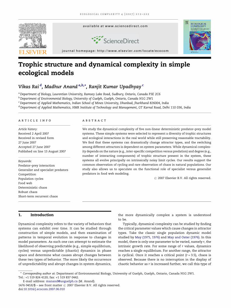
Fig. 1 – Points in 2D parameter space where chaos was observed in Model 1. Parameters varied: (a) 1.5 = a1 = 3.5;

50 = K = 200 with step size (0.05, 10); (b) 1 = A/c = 15; 1 = K1/D3 = 12 with step size (0.1, 0.1). (c) Time-series displaying

oscillatory and chaotic dynamics of the generalist predator U with two different initial conditions U0 = 10, 10.001 for (i) limit

cycle a1 = 2.5, A = 2.5, K1 = 200, w = 3 (ii) chaos a1 = 2, w = 3, A = 2, K1 = 100. Fixed values used for relevant cases: a1 = 2, a2 = 1,

w1 = 2, c = 0.2, w4 = 0.0257, w = 1, D = 10, D1 = 10, w2 = 0.05, D2 = 10, A = 1.5, K = 100, w3 = 0.74, D3 = 20.


generalist predators whose food requirements are quite low.

On the other hand, generalist predators with appreciable food

needs are better represented by the present version of the

model. We shall compare results of this model and those of Rai

(2004). The following schematic diagram represents the

model:

A real world ecological community that exemplifies this

model involves plantation, vole, weasel and its prey other

than the voles. This community is found in northern

Fennoscandia and has been studied by many investigators

(Turchin, 1996; Turchin and Hanski, 1997; Turchin and Ellner,

2000).

2.2. Model 2: two specialists, two competing prey

In this section, we design a model to represent an ecological

situation wherein two different prey are predated upon by two

different specialist predators. These two predator–prey sys-

tems with strong non-linear interactions are linked via

competition between the individuals of prey populations.

Vandermeer (2004) terms this as resource–resource (RR)

coupling. RR coupling essentially means indirect mutualism

between the two consumers (predators). Our aim is to

investigate the effect of this on two RM predator–prey systems.


The model is represented by following set of non-linear

coupled ordinary differential equations:

dX1

dt¼ a1X1 1� X1

K� X2

K1

� ��wY1X1

X1 þ D(4a)

dY1

dt¼ �a2Y1 þ

w1Y1X1

X1 þ D1(4b)

dX2

dt¼ a3X2 1� X2

K2� X1

K1

� ��w2Y2X2

X2 þ D2(4c)

dY2

dt¼ �a4Y2 þ

w3Y2X2

X2 þ D3; (4d)

The meaning of the symbols is the same as in Eqs. (1a) and (1b).

A population’s growth is limited either by the severity of

competition among its own individuals or/and by that of

competition among individuals of other species, which

depend on the same resource. K is the carrying capacity for

the prey species X1 and K2 for that of X2. K1 measures the

strength of interference competition between the two prey

species. The unit of K1 is number of individuals per unit

volume. The meaning of different symbols will be more clear

if one keeps in view the fact that this system is obtained by

coupling the two RM oscillators as shown in the following

schematic:

A real world community exemplifying this ecological

situation is Epirrita autumnata (a lepidopteran forest insect

pest) feeding on the plants in northern Fennoscandia and the

voles of the genera Microtus and Clethrionomys feedings on

another set of plants. The first herbivore system has 9-year

population cycle and the second system has a 5-year cycle

(Klemola et al., 2002).

2.3. Model 3: two competing specialists, two prey

Here we again design a model to examine the nature and

extent to which dynamics of an ecological system is

determined by coupling of two RM oscillators. In this case,

the predators can be thought of as specialized on a particular

prey, but consume an alternative prey on which another

predator specializes (MacArthur, 1970). Vandermeer (2004)

refers to this type of coupling as consumer–resource (CR)

coupling. CR coupling implies competition between two

predators. The model is represented by following set of

non-linear coupled differential equations:

dX1

dt¼ a1X1 1� X1

K

� ��wX1

Y1

1þ bðX1 þ bX2Þþ bY2

1þ bðX2 þ bX1Þ

� �

(5a)

dY1

dt¼ wðX1 þ bX2ÞY1

1þ bðX1 þ bX2Þ� a2Y1 (5b)

dX2

dt¼ a3X2 1� X2

K

� ��wX2

Y2

1þ bðX2 þ bX1Þþ bY1

1þ bðX1 þ bX2Þ

� �

(5c)

dY2

dt¼ wðX2 þ bX1ÞY2

1þ bðX2 þ bX1Þ� a4Y2; (5d)

where X1, X2 are the two prey and Y1, Y2 are corresponding

predators. These predators prey on each other’s prey. a1 and a3

are per capita reproductive growth rates for the prey X1 and X3.

K is the carrying capacity for the prey and b is the parameter

for the functional response of predators. Parameter b mea-

sures the strength of CR coupling. a2, a4 are mortality rates for

the two predators. The parameter w represents the consump-

tion rates of predators. The model is parameterized in such a

way that variables take any value between 0 and 1.

2.4. Model 4: one specialist, two competing prey

In this model, two prey species compete for the same resource

and each one is predated by the same specialist predator. We

thus consider switching behavior in the specialist predator, as

no predator is a specialist predator in the mathematical sense

encrypted in Eqs. (1a) and (1b). Some specialist predators do

switch to alternative prey when their most favorite food is in

short supply; e.g. lynx switches to red squirrel when snowshoe

hare becomes scarce (O’Donoghue et al., 1998), and the

Eurasian badger switches to rabbits when its preferred prey

(plants, worms and insects) becomes scarce (Fedriani et al.,

1998). The model is described by following equations:

dX1

dt¼ r1X1 1� X1

K1� c12X2

K1

� �� f1F1ðX1;X2ÞY (6a)

dX2

dt¼ r2X2 1� X2

K2� c21X1

K2

� �� f2F2ðX1;X2ÞY (6b)

dYdt¼ e1 f1F1ðX1;X2ÞY þ e2 f2F2ðX1;X2ÞY � dY; (6c)

where

f1 ¼pX1

pX1 þ ð1� pÞX2and f2 ¼

ð1� pÞX2

pX1 þ ð1� pÞX2;

where p is the prey preference and takes a value between 0

and 1.

FiðX1;X2Þ ¼AiXi

ð1þ B1X1 þ B2X2Þ;

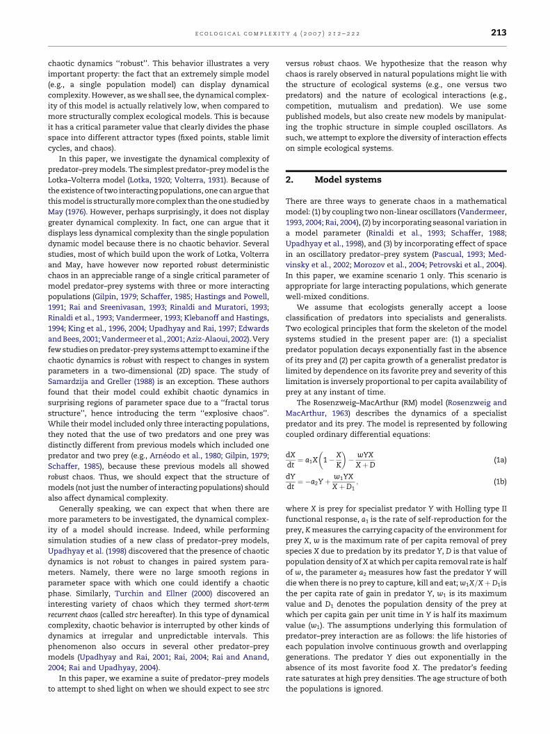
Fig. 2 – Points in 2D parameter space where chaos was

observed in Model 2. (a) 0.5 = a1 = 1.9; 30 = K1 = 65 with

step size (0.1, 5). (b) 0.2 = a2 = 0.8; 30 = K1 = 60 with step

size (0.05, 5) (c) 0.5 = a3 = 1.9; 30 = K1 = 60 with step size


where Ai is the maximum harvest rate of predator Y for prey Xi

and 1/Bi is proportional to the half-saturation constants. The

constants e1 and e2 are conversion rates of preyXi to predator Y.

Setting f1 and f2 equal to 1 in Eqs. (6a)–(6c), one gets the

system without switching. This system can be decoupled into

two RM oscillators (Rai, 2004). The two oscillators are

connected through inter-specific competition.

Gakkhar and Naji (2003) have discovered chaos in the

model without switching. However, scans of parameter space

were not presented in their publication. The assessment of

dynamical complexity is not possible without studying the

model in more detail. We performed simulation experiments

to investigate dynamical chaos in both versions of the model

(with and without switching).

2.5. Model 5: two generalists, two prey

This model is obtained by linking the two HT oscillators. It is

assumed that two generalist predators feed on both prey

species although they have their own favorite food items (X for

Y and Z for U). The model is represented by the following set of

differential equations:

dXdt¼ r1X 1� X

K1

� �� X

wY1þ Xþ aZ

þ aU1þ Xþ aZ

� �(7a)

dYdt¼ c1Y1 �

w2Y2

Xþ aZ(7b)

dZdt¼ r2Z 1� Z

K2

� �� Z

bY1þ Zþ bX

þ w1U1þ Zþ bX

� �(7c)

dUdt¼ c2U� w3U2

Zþ bX; (7d)

where parameters b and a are measures of intensity with

which two subsystems are connected to one another. Van-

dermeer (1993) called them parameters of connection asym-

metry (when b 6¼ a). r1, K1 and r2, K2 are per capita growth rates

and carrying capacities for the two prey. He found chaos for

a = 0.005 and b = 0.008. Here we present results of detailed

simulation experiments, which were performed in the spirit

of the methodology in Upadhyay et al. (2001).

Model 5 contains two types of parameters: (1) connection

asymmetry (a and b) and (2) driving asymmetry (r1, r2; K1, K2). The

(0.05, 5). Fixed values used for relevant cases: a2 = 1, a4 = 1,

a3 = 1.2, K = 35, K2 = 30, D = 10, D1 = 10, D2 = 15, D3 = 15,

w = 1, w1 = 2, w2 = 1, w3 = 2.


connection asymmetry parameters are measures of predation

intensity between the generalist predator and the other prey

(the one which is not its most favorite prey). On the other

hand, parameters of driving asymmetry are the per capita

reproductive rates and carrying capacities for the two prey. We

chose both kinds of parameters as control parameters to

perform simulation experiments.

3. Methodology

The model systems presented above are multi-parameter

systems. A few hundred parameter combinations (choosing

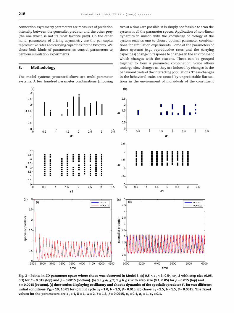
Fig. 3 – Points in 2D parameter space where chaos was observe

0.1) for b = 0.015 (top) and b = 0.0015 (bottom). (b) 0.5 = a1 = 3; 1

b = 0.0015 (bottom). (c) time-series displaying oscillatory and cha

initial conditions Y10 = 10, 10.01 for (i) limit cycle a1 = 1.0, b = 1.3

values for the parameters are a1 = 1, K = 1, w = 2, b = 1.3, b = 0.00

two at a time) are possible. It is simply not feasible to scan the

system in all the parameter spaces. Application of non-linear

dynamics in unison with the knowledge of biology of the

system enables one to choose optimal parameter combina-

tions for simulation experiments. Some of the parameters of

these systems (e.g., reproductive rates and the carrying

capacities) change in response to changes in the environment

which changes with the seasons. These can be grouped

together to form a parameter combination. Some others

undergo slow changes as they are induced by changes in the

behavioral traits of the interacting populations. These changes

in the behavioral traits are caused by unpredictable fluctua-

tions in the environment of individuals of the constituent

d in Model 3. (a) 0.5 = a1 = 3; 0:5�� w�� 3 with step size (0.05,

= b = 2 with step size (0.1, 0.05) for b = 0.015 (top) and

otic dynamics of the specialist predator Y1 for two different

, b = 0.015, (ii) chaos a1 = 2.5, b = 1.5, b = 0.0015. The Fixed

15, a2 = 0.1, a3 = 1, a4 = 0.1.


populations. To fix the ranges of parameters appearing in

parameter combinations for simulation experiments, we use

the method suggested by Upadhyay et al. (1998). The system of

equations is integrated using standard numerical procedures

to generate time-histories for a given set of parameter values.

The distinguishing property of chaos is sensitive dependence

on initial conditions. Two initially close trajectories in the state

space (or in the phase space) diverge exponentially fast to the

extent that after elapse of a certain amount of time, the two

appear to originate from two different dynamical systems. We

choose this basic feature of chaotic dynamics to detect the

presence as well as absence of chaos in these model systems.

The system parameters are chosen in such a way that

asymptotic dynamics of both the subsystems confine to a

stable limit cycle. If the two time-histories (generated by

integrating the system of differential equations and recorded

after transients are died out) corresponding to two different,

but very close, initial conditions overlap each other comple-

tely, the absence of dynamical chaos at that particular set of

Fig. 4 – Points in 2D parameter space where chaos was observed

switching behavior. For (a): (i) 0.5 = r1 = 4.5; 50 = K2 = 350 with s

(0.2, 10). The parameter values for limit cycle solutions are: r1 =

c12 = 0.204, C21 = 0.208, d = 1.21, B1 = 0.54, B2 = 0.55, e1 = 2.5, e2 = 0

25). (ii) 1.5 = r2 = 4; 50 = K1 = 250 with step size (0.25, 25). The pa

K1 = 150, K2 = 155, A1 = 1.1, A2 = 0.26, c12 = 1.1, c21 = 0.2, d = 1.2, B

parameter values is inferred. In the case when two histories

appear to be quite different, it is understood that chaos exists

at the chosen set of parameter values. There is one more

important aspect of these simulation experiments: choosing

the step size for the variation of a system parameter from a

parameter combination within the chosen range. This

depends on the nature of the parameter concerned (whether

it is a slow varying or fast varying one).

We chose the range of the two critical parameters based on

the available information about the parameters (Jorgensen,

1979), which are intrinsic attributes of the system. The critical

parameters are varied one at a time in the chosen range. ODE

Workbench from AIP (IBM PC Version 1.5; Aguirregabiria, 1994)

was used to integrate the system of differential equations

numerically. Dormance and Prince 5 (Hairer et al., 1993) was

the integration algorithm chosen for the purpose. Comparing

two time histories is the most simple and efficient way of

detecting the presence as well as absence of chaos in model

dynamical systems. This enables one to study two forms of

in Model 4 without switching behavior ( f1, f2 = 1) and with

tep size (0.1, 10). (ii) 1 = r2 = 4; 50 = K1 = 250 with step size

2.6, r2 = 2.65, K1 = 150, K2 = 155, A1 = 1.06, A2 = 0.35,

.52. For (b) (i) 1 = r1 = 2.8; 50 = K2 = 350 with step size (0.1,

rameter values for limit cycle solutions are: r1 = 2.6, r2 = 2.1,

1 = 0.54, B2 = 0.01, e1 = 2.5, e2 = 0.52, p = 0.5.


chaos in dissipative dynamical systems (dynamical chaos as

well as intermittent chaos) (Berge et al., 1986; Vandermeer,

1993; Letellier and Aziz-Alaoui, 2002). Of course, the method is

not helpful to distinguish between long-lived chaotic tran-

sients and chaotic dynamics on a bonafide chaotic attractor.

The phenomenon of chaotic transients (Grebogi et al., 1983;

Rai and Schaffer, 2001) is more prevalent in spatially extended

systems, which we do not study in the present paper. We also

mention that we did not use the maximum Lyapunov

exponent to detect chaos in the models we studied because

the method we chose was time saving. Moreover, a positive

maximum Lyapunov exponent does not guarantee dynamical

chaos even in a deterministic system (Alligood et al., 1997). Of

course, one has to take precautions to detect weak chaos using

this methodology. A large number of data points are thrown

out as transients so that there is sufficient time for chaos to

develop.

We (Rai, 2004; Rai and Upadhyay, 2004) have classified

dynamical complexity into two main categories: (1) robust

chaos and (2) short-term recurrent chaos (strc). When one finds

dynamical chaos to exist in a densely populated region defined

by two control parameters of the system, a case for robust

chaos is encountered. On the other hand, strc manifests itself

as a scatter of points in 2D parameter spaces. Extensive

simulation experiments were performed in 2D parameter

spaces spanned by per capita reproductive rate (a1) and

carrying capacity (K) of prey X; death rate (a2) and the foraging

efficiency ðw1Þ of the specialist predator; per capita reproduc-

tive rate (c) and a measure of dependence of the generalist

predator on its most favorite prey ðw4Þ to mention a few.

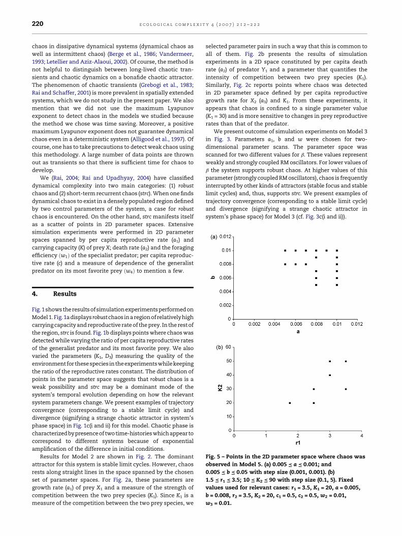
Fig. 5 – Points in the 2D parameter space where chaos was

observed in Model 5. (a) 0.005 = a = 0.001; and

0.005 = b = 0.05 with step size (0.001, 0.001). (b)

1.5 = r1 = 3.5; 10 = K2 = 90 with step size (0.1, 5). Fixed

values used for relevant cases: r1 = 3.5, K1 = 20, a = 0.005,

b = 0.008, r2 = 3.5, K2 = 20, c1 = 0.5, c2 = 0.5, w2 = 0.01,

w3 = 0.01.

4. Results

Fig.1showstheresultsofsimulationexperimentsperformedon

Model1.Fig.1adisplays robustchaos inaregionofrelativelyhigh

carrying capacity and reproductive rate of the prey. In the rest of

the region, strc is found. Fig. 1b displays points where chaos was

detected while varying the ratio of per capita reproductive rates

of the generalist predator and its most favorite prey. We also

varied the parameters (K1, D3) measuring the quality of the

environmentfor thesespecies intheexperimentswhilekeeping

the ratio of the reproductive rates constant. The distribution of

points in the parameter space suggests that robust chaos is a

weak possibility and strc may be a dominant mode of the

system’s temporal evolution depending on how the relevant

system parameters change. We present examples of trajectory

convergence (corresponding to a stable limit cycle) and

divergence (signifying a strange chaotic attractor in system’s

phase space) in Fig. 1c(i and ii) for this model. Chaotic phase is

characterizedbypresenceoftwotime-historieswhichappearto

correspond to different systems because of exponential

amplification of the difference in initial conditions.

Results for Model 2 are shown in Fig. 2. The dominant

attractor for this system is stable limit cycles. However, chaos

rests along straight lines in the space spanned by the chosen

set of parameter spaces. For Fig. 2a, these parameters are

growth rate (a1) of prey X1 and a measure of the strength of

competition between the two prey species (K1). Since K1 is a

measure of the competition between the two prey species, we

selected parameter pairs in such a way that this is common to

all of them. Fig. 2b presents the results of simulation

experiments in a 2D space constituted by per capita death

rate (a2) of predator Y1 and a parameter that quantifies the

intensity of competition between two prey species (K1).

Similarly, Fig. 2c reports points where chaos was detected

in 2D parameter space defined by per capita reproductive

growth rate for X2 (a3) and K1. From these experiments, it

appears that chaos is confined to a single parameter value

(K1 = 30) and is more sensitive to changes in prey reproductive

rates than that of the predator.

We present outcome of simulation experiments on Model 3

in Fig. 3. Parameters a1, b and w were chosen for two-

dimensional parameter scans. The parameter space was

scanned for two different values for b. These values represent

weakly and strongly coupled RM oscillators. For lower values of

b the system supports robust chaos. At higher values of this

parameter (strongly coupled RM oscillators), chaos is frequently

interrupted by other kinds of attractors (stable focus and stable

limit cycles) and, thus, supports strc. We present examples of

trajectory convergence (corresponding to a stable limit cycle)

and divergence (signifying a strange chaotic attractor in

system’s phase space) for Model 3 (cf. Fig. 3c(i and ii)).


Fig. 4 shows the results of our simulation experiments on

Model 4. We explored parameter spaces spanned by r1, K2 and

r2, K1. Results simulation experiments are presented in Figure

(a) without and (b) with switching in the diet of the predator.

We found few and intermittent occurrences of chaos in

general, and in the case of switching, no chaos was observed in

the parameter scan in r2 � K1 space.

Results of simulation experiments to study presence and

absence of chaos in Model 5 is presented in Fig. 5. In these

experiments, one connection parameter was varied at a time

(cf. Fig. 5a). We also study presence and absence of chaos in

this model system by varying r1 and K2 (Fig. 5b).

5. Discussion and conclusion

In all the models we studied chaotic dynamics is interrupted by

predictable changes in system parameters. The deterministic

change in system parameters is to be contrasted with stochastic

environmental influences that act on initial conditions.

Seasonality is one of the agencies causing these deterministic

changes in system parameters (reproductive rates and carrying

capacities). Even if one discovers a way to deal with the impact

of long-term environmental fluctuations so as to get a suitable

time-series which can be analyzed using concepts and

techniques fromnon-linear time series analysisand forecasting

(Turchin and Ellner, 2000), the likelihood that an unambiguous

case for chaos will be found is small. The on–off character of

chaos will render its capture in the wild elusive. In the presence

(and absence) of exogenous environmental perturbations,

ecological systems will display short-term recurrent chaos

(Turchin and Ellner, 2000; Rai, 2004; Rai and Upadhyay, 2004,

2006). The challenge remains the same: to distinguish between

deterministic chaos and noisy periodicity (Olsen and Schaffer,

1990; Kendall, 2001; Rai and Schaffer, 2001). We emphasize that

the source of this challenge is frequent interruptions in chaotic

dynamics caused by non-linear interactions.

We found that in most of the models, the dominant

behavior found was stable limit cycles. We hypothesize that

the coupling between the dynamics of specialist non-

competing predators (herbivorous insects and small mam-

mals, e.g., voles) and their prey (e.g., different varieties of

plants) explains pronounced population cycles observed in

many predator–prey systems, for example the herbivores in

northern Fennoscandia (Klemola et al., 2002). No population-

extrinsic condition is needed to understand the differences

between these observed cycles and ideal cycles. In harsh

environments experiencing strong seasonality, the inter-

specific competition between different prey (functional

varieties of plants) may be severe enough to put the parameter

(K1) at high values. Thus, occasional chaotic bursts can explain

the apparent departures from ideal cycles observed in real

population dynamics.

Our study allows us to make some comments about the

relationship between trophic structure and dynamical com-

plexity. It appears that the most complex models (Models 1

and 3) displayed dynamical complexity (in the form of strc). It is

interesting to note that Model 1 is the only one that

incorporates both generalist and specialist predators. This

provides a nice complement to results of Fussman and Heber

(2002) who showed that the frequency of chaotic dynamics

increases with the number of trophic levels (they did not

differentiate between generalist and specialist predators). If

we compare the results from an earlier work on a different

version of Model 1, which assumes that the switching to

alternative prey in the generalist predator’s foraging strategy

is infrequent (Rai, 2004), we find that the system’s tendency to

exhibit episodes of chaotic dynamics is considerably increased

(cf. description of Model 1 in Section 2.1). Model 2 contains two

specialist predators whose prey are in competition with each

other. In this model, we see a few points where chaotic

dynamics exists. This suggests that most likely outcome of

models involving the same kind of predators (either the

specialist or generalist) in natural systems is cycles not chaos.

This could be an explanation for the abundance of population

cycles in nature (Kendall et al., 1999). Of course, the observed

dynamical patterns will not conform to ideal cycles. These

departures are caused by existence of chaotic dynamics in

some (albeit small) regions of the parameter space. Thus, non-

linear interactions, and not exogenous environmental factors

could explain observations of these deviations from ideal

cycles. It is interesting to note that coupling two generalists

(Model 5) shows more points of observation of chaos than

coupling two specialist predators (Model 2) and the model with

one specialist predator with switching in its diet (Model 4).

This suggests that the generalist behavior may be functionally

important for dynamical complexity in these types of systems

(Tanabe and Namba, 2005).

Acknowledgements

M.A. acknowledges financial support from a Canada Research

Chair and Discovery grant (Natural Sciences and Engineering

Council of Canada) and the Ontario Ministry of Economic

Development and Trade (Science and Technology Division) to

undertake this collaborative project. V.R. gratefully acknowl-

edges the Department of Biology at Laurentian University for

hosting his 4-month visit and Bai-Lian (Larry) Li for helpful

discussions during a brief visit to his lab. R.U. acknowledges

financial support from D.S.T., Government of India.

r e f e r e n c e s

Aguirregabiria, J.M., 1994. ODE Workbench. Physics AcademicSoftware.

Alligood, K.T., Sauer, T.D., Yorke, J.A., 1997. Chaos: AnIntroduction to Dynamical Systems. Springer, Berlin,Germany.

Arneodo, A., Coullet, P., Tresser, C., 1980. Occurrence of strangeattractors in three-dimensional Volterra equation. Phys.Lett. 79A, 259–263.

Aziz-Alaoui, M.A., 2002. Study of a Leslie–Gower type tri-trophicpopulation model. Chaos Solitons Fract. 14 (8), 1275–1293.

Berge’, P., Pomeau, Y., Vidal, C., 1986. Order Within Chaos:Towards a Deterministic Approach to Turbulence. JohnWiley & Sons, NY, USA.

Edwards, A.M., Bees, M.A., 2001. Generic dynamics of a simpleplankton population model with a non-integer exponent ofclosure. Chaos Solitons Fract. 12 (2), 289–300.


Fedriani, J.M., Ferreras, P., Delibes, M., 1998. Dietary response ofthe Eurasian badger, Meles meles, to a decline of its mainprey in the Donana National Park. J. Zool. 245, 214–218.

Fussman, G.F., Heber, G., 2002. Food web complexity and chaoticpopulation dynamics. Ecol. Lett. 5, 394–401.

Gakkhar, S., Naji, R.K., 2003. Existence of chaos in two-prey, onepredator system. Chaos Solitons Fract. 17, 639–649.

Gilpin, M.E., 1979. Spiral chaos in a predator–prey model. Am.Nat. 113, 306–308.

Grebogi, C., Ott, E., Yorke, J.A., 1983. Crises, sudden changes inchaotic attractors and transient chaos. Phys. D 7, 181–200.

Hastings, A., Powell, T., 1991. Chaos in a three-species foodchain. Ecology 72, 896–903.

Hairer, E., Norsett, S.P., Wanner, G., 1993. Solving DifferentialEquations I: Nonstiff Problems, 2nd ed. Springer, Berlin.

Holling, C.S., 1965. The functional response of invertebratepredators to prey density. Mem. Entomol. Soc. Can. 45, 3–60.

Jorgensen, S.E., 1979. Handbook of Environmental Data andEcological Parameters. Pergamon Press, Amsterdam.

Kendall, B.E., 2001. Cycles, chaos and noise in predator–preydynamics. Chaos Solitons Fract. 12, 321–332.

Kendall, B.E., Briggs, C.J., Murdock, W.W., Turchin, P., Ellner,S.P., McCauley, E., Nisbet, R.M., Wood, S.N., 1999. Why dopopulations cycle? A synthesis of statistic and mechanicalmodeling approaches. Ecology 80, 1789–1805.

King, A.A., Schaffer, W.M., Gordon, C., Treat, J., Kot, M., 1996.Weakly dissipative predator–prey systems. Bull. Math. Biol.58, 835–859.

King, A.A., Costantino, R.F., Cushing, J.M., Henson, S.M.,Desharnais, R.A., Denis, B., 2004. Anatomy of a chaoticattractor: subtle model predicted patterns revealed inpopulation data. Proc. Natl. Acad. Sci. U.S.A. 101, 408–413.

Klebanoff, A., Hastings, A., 1994. Chaos in three species foodchains. J. Math. Biol. 32, 427–451.

Klemola, T., Tanhuanpaa, M., Korpimaki, E., Ruohomaki, K.,2002. Specialist and generalist natural enemies as anexplanation for geographical gradients in population cyclesof northern herbivores. Oikos 99, 83–94.

Letellier, C., Aziz-Alaoui, M.A., 2002. Analysis of the dynamics ofa realistic ecological model. Chaos Solitons Fract. 13, 95–107.

Lotka, A.J., 1920. Undamped oscillations derived from the law ofmass action. J. Am. Chem. Soc. 42, 1595.

MacArthur, R.H., 1970. Species packing and competitiveequilibrium for many species. Theor. Pop. Biol. 1, 1–11.

May, R.M., 1975. Biological populations obeying differenceequations: simple points, stable cycles, and chaos. J. Theor.Biol. 49, 511–524.

May, R.M., 1976. Simple mathematical models with verycomplicated dynamics. Nature 261, 459–467.

May, R.M., Oster, G.F., 1976. Bifurcation and dynamic complexityin simple ecological models. Am. Nat. 110, 578–599.

May, R.M., 2001. Stability and Complexity in Model Ecosystems.Princeton University Press, Princeton, New Jersey.

Medvinsky, A.B., Petrovskii, S.V., Tikhonova, I.A., Malchow, H.,Li, B.-L., 2002. Spatio-temporal complexity of plankton andfish dynamics. SIAM Rev. 44, 311–370.

Morozov, A., Petrovski, S., Li, B.-L., 2004. Bifurcations and chaosin a predator–prey system with Allee effect. Proc. R. Soc.Lond. B 271, 1407–1414.

O’Donoghue, M., Boutin, S., Krebs, C.J., Zuleta, G., Murray, D.L.,Hofer, E.J., 1998. Functional response of coyotes and lynx tothe snowshoe hare cycle. Ecology 79, 1193–1208.

Olsen, L.F., Schaffer, W.M., 1990. Chaos versus noisy periodicity:alternative hypotheses for childhood epidemics Science249, 499–504.

Pascual, M., 1993. Diffusion-induced chaos in a spatial predator–prey system. Proc. R. Soc. Lond. B 251, 1–7.

Pielou, E.C., 1977. Mathematical Ecology: An Introduction.Wiley, NY, USA.

Petrovski, S., Li, B.-L., Malchow, H., 2004. Transition tospatiotemporal chaos can resolve the paradox ofenrichment. Ecol. Complexity 1, 37–47.

Rai, V., Sreenivasan, R., 1993. Period doubling bifurcationsleading to chaos in a model food-chain. Ecol. Model. 69,63–77.

Rai, V., Schaffer, W.M., 2001. Chaos in ecology. Chaos SolitonsFract. 12, 197–203.

Rai, V., 2004. Chaos in natural populations: edge or wedge? Ecol.Complexity 1 (2), 127–138.

Rai, V., Anand, M., 2004. Is dynamic complexity of ecologicalsystems quantifiable? Int. J. Ecol. Env. Sci. 30, 123–130.

Rai, V., Upadhyay, R.K., 2004. Chaotic population dynamics andthe biology of the top-predator. Chaos Solitons Fract. 21,1195–1204.

Rai, V., Upadhyay, R.K., 2006. Evolving to the edge of chaos:chance or necessity? Chaos Solitons Fract. 30, 1074–1087.

Rinaldi, S., Muratori, S., 1993. Conditioned chaos in seasonallyperturbed predator–prey models. Ecol. Model. 69, 79–97.

Rinaldi, S., Muratori, S., Kuznetsov, Y., 1993. Multiple attractors,catastrophes and chaos in seasonally perturbed predator–prey communities. Bull. Math. Biol. 55, 15–35.

Rosenzweig, M.L., MacArthur, R.H., 1963. Graphicalrepresentation and stability conditions of predator–preyinteractions. Am. Nat. 97, 209–223.

Schaffer, W.M., 1985. Order and chaos in ecological systems.Ecology 66, 93–106.

Schaffer, W.M., 1988. Perceiving order in the chaos of nature. In:Boyce, M. (Ed.), Life Histories: Theory and Patterns fromMammals. Yale University Press, New Haven, pp. 313–350.

Samardzija, N., Greller, L.D., 1988. Explosive route to chaosthrough a fractal torus in a generalized Lotka–Volterramodel. Bull. Math. Biol. 50 (5), 465–491.

Tanabe, K., Namba, T., 2005. Omnivory creates chaos in simplefood web models. Ecology 86 (12), 3411–3414.

Tanner, J.T., 1975. The stability and intrinsic growth rates ofprey and predator populations. Ecology 56, 855–867.

Turchin, P., 1996. Non-linear time-series modeling of volepopulation fluctuations. Res. Pop. Ecol. 38, 121–132.

Turchin, P., Hanski, I., 1997. An empirically-based model for thelatitudinal gradient in vole population dynamics. Am. Nat.149, 842–874.

Turchin, P., Ellner, S.P., 2000. Living on the edge of chaos:population dynamics of Fennoscandian voles. Ecology 81,3099–3116.

Upadhyay, R.K., Rai, V., 1997. Why chaos is rarely observed innatural populations? Chaos Solitons Fract. 8, 1933–1939.

Upadhyay, R.K., Iyengar, S.R.K., Rai, V., 1998. Chaos: anecological reality? Int. J. Bifur. Chaos 8, 1325–1333.

Upadhyay, R.K., Rai, V., 2001. Crisis-limited chaotic dynamics inmodel ecological systems. Chaos Solitons Fract. 12,205–218.

Upadhyay, R.K., Rai, V., Iyengar, S.R.K., 2001. Species extinctionproblem: genetic vs. ecological factors. Appl. Math. Model.25, 937–951.

Vandermeer, J., 1993. Loose coupling of predator–prey cycles:entrainment, chaos and intermittency in the classicalMacArthur consumer–resource equations. Am. Nat. 141,687–716.

Vandermeer, J., Stone, L., Blasius, B., 2001. Categories of chaosand fractal basin boundaries in forced predator–preymodels. Chaos Solitons Fract. 12 (2), 265–276.

Vandermeer, J., 2004. Coupled oscillations in food webs:balancing competition and mutualism in simple ecologicalmodels. Am. Nat. 163, 857–867.

Volterra, V., 1931. Variations and fluctuations of the number ofindividuals in animal species living together. In: AnimalEcology, McGraw-Hill, Translated from 1928 edition by R.N.Chapman.

trophic structure and dynamical complexity in simple ecological models

Documents