Tridirectional Typechecking

Joshua Dunfield Frank Pfenning

March 26, 2004CMU-CS-04-117

School of Computer ScienceCarnegie Mellon University

Pittsburgh, PA 15213

Abstract

In prior work we introduced a pure type assignment system that encompasses a rich set of prop-erty types, including intersections, unions, and universally and existentially quantified depen-dent types. This system was shown sound with respect to a call-by-value operational semanticswith effects, yet is inherently undecidable. In this paper we provide a decidable formulation forthis system based on bidirectional checking, combining type synthesis and analysis followinglogical principles. The presence of unions and existential quantification requires the additionalability to visit subterms in evaluation position before the context in which they occur, leading to atridirectional type system. While soundness with respect to the type assignment system is imme-diate, completeness requires the novel concept of contextual type annotations, introducing a notionfrom the study of principal typings into the source program.

This is an extended version of [DP04].

This work supported in part by the National Science Foundation under grant CCR-0204248 Type Refine-ments; the first author was also supported in part by an NSF Graduate Research Fellowship. Any opinions,findings, conclusions or recommendations expressed in this publication are those of the authors and do notnecessarily reflect the views of the National Science Foundation.

Keywords: Type systems, intersection types, union types, type refinements, bidirectionaltypechecking, datasort refinements, index refinements

1

1 Introduction

Over the last two decades, there has been a steady increase in the use of type systems to captureprogram properties such as control flow [PP01], memory management [TT97], aliasing [SWM00],data structure invariants [FP91, DP00, XP99] and effects [TJ94, MWH02], to mention just a few.Ideally, such type systems specify rigorously, yet at a high level of abstraction, how to reasonabout a certain class of program properties. This specification usually serves a dual purpose: it isused to relate the properties of interest to the operational semantics of the programming language(for example, proving type preservation), and it is the basis for concrete algorithms for programanalysis (for example, via constraint-based type inference).

While the type-based approach has been successful for use in automatic program analysis(for example, for optimization during compilation), it has been less successful in making theexpressive type systems directly available to the programmer. One reason for this is the difficultyof finding the right balance between the brevity of the additional required type declarations andthe feasibility of the typechecking problem. Another is the difficulty of giving precise and usefulfeedback to the programmer on ill-typed programs.

In prior work [DP03] we developed a system of pure type assignment designed for call-by-value languages with effects and proved progress and type preservation. The intended atomicprogram properties are data structure refinements [FP91, Fre94, XP99], but our approach does notdepend essentially on this choice. Atomic properties can be combined into more complex onesthrough intersections, unions, and universal and existential quantification over index domains.As a pure type assignment system, where terms do not contain any types at all, it is inherentlyundecidable [CDCV81].

In this paper we develop an annotation discipline and typechecking algorithm for our earliertype assignment system. The major contribution is the type system itself which contains severalnovel ideas, including an extension of the paradigm of bidirectional typechecking to union andexistential types, leading to the tridirectional system. While type soundness follows immediatelyby erasure of annotations, completeness requires that we insert contextual typing annotations rem-iniscent of principal typings [Jim95, Wel02]. Decidability is not obvious; we prove it by showingthat a slightly altered left tridirectional system is decidable (and sound and complete with respectto the tridirectional system).

The basic underlying idea is bidirectional checking [PT98] of programs containing some typeannotations, combining type synthesis with type analysis, first adapted to property types by Daviesand Pfenning [DP00]. Synthesis generates a type for a term from its immediate subterms. Log-ically, this is appropriate for destructors (or elimination forms) of a type. For example, the firstproduct elimination passes from e : A ∗ B to fst(e) : A. Therefore, if we can generate A ∗ B we canextract A. Dually, analysis verifies that a term has a given type by verifying appropriate types forits immediate subterms. Logically, this is appropriate for constructors (or introduction forms) of atype. For example, to verify that λx. e : A → B we assume x : A and then verify e : B. Bidirectionalchecking works for both the native types of the underlying programming language and the layerof property types we construct over it.

However, the simple bidirectional model is not sufficient for what we call indefinite propertytypes: unions and existential quantification. This is because the program lacks the prerequisitestructure. For example, if we synthesize A ∨ B, the union of A and B, for an expression e, wenow need to distinguish the cases: the value of e might have type A or it might have type B. De-termining the proper scope of this case distinction depends on how e is used, that is, the positionin which e occurs. This means we need a “third direction” (whence the name tridirectional): wemight need to move to a subexpression, synthesize its type, and only then analyze the expressionsurrounding it.

Since the tridirectional type system (like the bidirectional one) requires annotations, we wantto know that any program well typed in the type assignment system can be annotated so that it

2 2 THE CORE LANGUAGE

is also well typed in the tridirectional system. But with intersection types, such a completenessproperty does not hold for the usual notion of type annotation (e : A) (as previously noted [Pie91a,Dav97b, WH02]), a problem exacerbated by scoping issues arising from quantified types. Wetherefore extend the notion of type annotation to contextual typing annotation, (e : Γ1 ` A1, . . . , Γn `An), in which the programmer can write several context/type pairs. The idea is that an annota-tion Γk ` Ak may be used when e is checked in a context matching Γk. This idea might also beapplicable to arbitrary rank polymorphism, a possibility we plan to explore in future work.

Unlike the bidirectional system, the indefinite property types that necessitate the third direc-tion make decidability of typechecking nontrivial. Two ideas come to the rescue. First, to preservetype safety in a call-by-value language with effects, the type of a subterm e can only be broughtout if the term containing it has the form E[e] for some evaluation context E, reducing the nonde-terminism; this was a key observation in our earlier paper [DP03]. Second, one never needs tovisit a subterm more than once in the same derivation: the system which enforces this is soundand complete.

The remainder of the paper is organized as follows. Section 2 presents a simple bidirectionaltype system. Section 3 adds refinements and a rich set of types including intersections and unions,using tridirectional rules; this is the simple tridirectional system. In Section 4, we explain our formof typing annotation and prove that the simple tridirectional system is complete with respectto the type assignment system. Section 5 restricts the tridirectional rules and compensates byintroducing left rules to yield a left tridirectional system. We prove soundness and completenesswith respect to the simple tridirectional system, prove decidability, and use the results in [DP03]to prove type safety. Finally, we discuss related work (Section 6) and conclude (Section 7).

The report vs. the paper. This report is an extended version of our POPL ’04 paper [DP04].Besides full proofs, it contains a number of remarks omitted in the paper. Consequently, thenumbering of theorems differs.

2 The Core Language

In a pure type assignment system, the typing judgment is e : A, where e contains no types (elidingcontexts for the moment). In a bidirectional type system, we have two typing judgments: e ↑ A,read e synthesizes A, and e ↓ A, read e checks against A. The most straightforward implementationof such a system consists of two mutually recursive functions: the first, corresponding to e ↑ A,takes the term e and either returns A or fails; the second, corresponding to e ↓ A, takes the terme and a type A and succeeds (returning nothing) or fails. This raises a question: Where do thetypes in the judgments e ↓ A come from? More generally: what are the design principles behinda bidirectional type system?

Avoiding unification or similar techniques associated with full type inference is fundamentalto the design of the bidirectional system we propose here. The motivation for this is twofold. First,for highly expressive systems such as the ones under consideration here, full type inference isoften undecidable, so we need less automatic and more robust methods. Second, since unificationglobally propagates type information, it is often difficult to pinpoint the source of type errors.

We think of the process of bidirectional typechecking as a bottom-up construction of a typ-ing derivation, either of e ↑ A or e ↓ A. Given that we want to avoid unification and similartechniques, we need each inference rule to be mode correct, terminology borrowed from logic pro-gramming. That is, for any rule with conclusion e ↑ A we must be able to determine A from theinformation in the premises. Conversely, if we have a rule with premise e ↓ A, we must be ableto determine A before traversing e.

3

However, mode correctness by itself is only a consistency requirement, not a design principle.We find such a principle in the realm of logic, and transfer it to our setting. In natural deduction,we distinguish introduction rules and elimination rules. An introduction rule specifies how to infera proposition from its components; when read bottom-up, it decomposes the proposition. Forexample, the introduction rule for the conjunction A ∗ B decomposes it to the goals of proving A

and B. Therefore, a rule that checks a term against A ∗ B using an introduction rule will be modecorrect.

Γ ` e1 ↓ A1 Γ ` e2 ↓ A2

Γ ` (e1, e2) ↓ A1 ∗ A2(∗I)

Conversely, an elimination rule specifies how to use the fact that a certain proposition holds;when read top-down, it decomposes a proposition. For example, the two elimination rules forthe conjunction A ∗ B decompose it to A and B, respectively. Therefore, a rule that infers a typefor a term using an elimination rule will be mode correct.

Γ ` e ↑ A ∗ B

Γ ` fst(e) ↑ A(∗E1)

Γ ` e ↑ A ∗ B

Γ ` snd(e) ↑ B(∗E2)

If we employ this design principle throughout, the constructors (corresponding to the introduc-tion rules) for the elements of a type are checked against a given type, while the destructors (corre-sponding to the elimination rules) for the elements of a type synthesize their type. This leads to thefollowing rules for functions, in which rule (→I) checks against A → B and rule (→E) synthesizesthe type A → B of its subject e1

Γ, x:A ` e ↓ B

Γ ` λx. e ↓ A → B(→I)

Γ ` e1 ↑ A → B Γ ` e2 ↓ A

Γ ` e1(e2) ↑ B(→E)

What do we do when the different judgment directions meet? If we are trying to check e ↓ A thenit is sufficient to synthesize a type e ↑ A ′ and check that A ′ = A. More generally, in a system withsubtyping, it is sufficient to know that every value of type A ′ also has type A, that is, A ′ ≤ A.

Γ ` e ↑ A ′ Γ ` A ′ ≤ A

Γ ` e ↓ A(sub)

In the opposite direction, if we want to synthesize a type for e but can only check e against agiven type, then we do not have enough information. In the realm of logic, such a step wouldcorrespond to a proof that is not in normal form (and might not have the subformula property).The straightforward solution would be to allow source expressions (e : A) via a rule

Γ ` e ↓ A

Γ ` (e : A) ↑ A

Unfortunately, this is not general enough due to the presence of intersections and universallyand existentially quantified property types. We discuss the issues and our solution in detail inSection 4. For now, only normal terms will typecheck in our system. These correspond exactlyto normal proofs in natural deduction. We can therefore already pinpoint where annotations willbe required in the full system: exactly where the term is not normal. This will be the case wheredestructors are applied to constructors (that is, as redexes) and at certain let forms.

In addition we permit datatypes δ with constructors c(e) and corresponding case expressionscase e of ms, where the match expressions ms have the form c1(x1) ⇒ e1| . . . cn(xn) ⇒ en.The constants c are the constructors and case the destructor of elements of type δ. This meansexpressions c(e) are checked against a type, while the subject of a case must synthesize its type.Assuming constructors have type A → δ, this yields the following rules.

c : A → δ Γ ` e ↓ A

Γ ` c(e) ↓ δ(δI)

Γ ` e ↑ δ Γ ` ms ↓δ B

Γ ` case e of ms ↓ B(δE)

Γ ` · ↓δ C

c : A → δ Γ, x:A ` e ↓ B Γ ` ms ↓δ B

Γ ` c(x) ⇒ e |ms ↓δ B

4 2 THE CORE LANGUAGE

Types A, B, C, D ::= 1 | A → B | A ∗ B | δ

Terms e ::= x | u | λx. e | e1 e2 | fix u. e

| () | (e1, e2) | fst(e) | snd(e)

| c(e) | case e of ms

Matches ms ::= · | c(x) ⇒ e|ms

Values v ::= x | λx. e | () | (v1, v2)

Eval. contexts E ::= [ ] | E(e) | v(E)

| (E, e) | (v, E) | fst(E) | snd(E)

| c(E) | case E of ms

e ′ 7→R e ′′

E[e ′] 7→ E[e ′′]

(λx. e) v 7→R [v/x] e fst(v1, v2) 7→R v1

fix u. e 7→R [fix u. e / u] e snd(v1, v2) 7→R v2

case c(v) of . . . c(x) ⇒ e . . . 7→R [v/x] e

Figure 1: Syntax and semantics of the core language

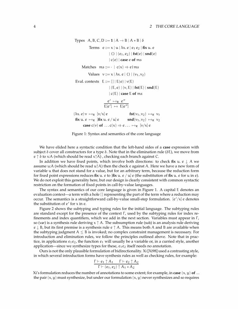
We have elided here a syntactic condition that the left-hand sides of a case expression withsubject δ cover all constructors for a type δ. Note that in the elimination rule (δE), we move frome ↑ δ to x:A (which should be read x↑A) , checking each branch against C.

In addition we have fixed points, which involve both directions: to check fix u. e ↓ A weassume u:A (which should be read u↑A) then the check e against A. Here we have a new form ofvariable u that does not stand for a value, but for an arbitrary term, because the reduction formfor fixed point expressions reduces fix u. e to [fix u. e / u] e (the substitution of fix u. e for u in e).We do not exploit this generality here, but our design is clearly consistent with common syntacticrestriction on the formation of fixed points in call-by-value languages.

The syntax and semantics of our core language is given in Figure 1. A capital E denotes anevaluation context—a term with a hole [ ] representing the part of the term where a reduction mayoccur. The semantics is a straightforward call-by-value small-step formulation. [e ′/x] e denotesthe substitution of e ′ for x in e.

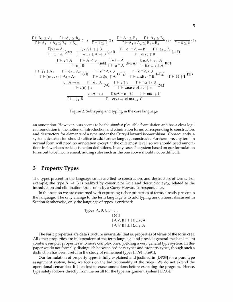
Figure 2 shows the subtyping and typing rules for the initial language. The subtyping rulesare standard except for the presence of the context Γ , used by the subtyping rules for index re-finements and index quantifiers, which we add in the next section. Variables must appear in Γ ,so (var) is a synthesis rule deriving x ↑ A. The subsumption rule (sub) is an analysis rule derivinge ↓ B, but its first premise is a synthesis rule e ↑ A. This means both A and B are available whenthe subtyping judgment A ≤ B is invoked; no complex constraint management is necessary. Forintroduction and elimination rules, we follow the principles outlined above. Note that in prac-tice, in applications e1e2, the function e1 will usually be a variable or, in a curried style, anotherapplication—since we synthesize types for these, e1e2 itself needs no annotation.

Ours is not the only plausible formulation of bidirectionality. Xi [Xi98] used a contrasting style,in which several introduction forms have synthesis rules as well as checking rules, for example:

Γ ` e1 ↑ A1 Γ ` e2 ↑ A2

Γ ` (e1, e2) ↑ A1 ∗ A2

Xi’s formulation reduces the number of annotations to some extent; for example, in case (x, y) of ...

the pair (x, y) must synthesize, but under our formulation (x, y) never synthesizes and so requires

5

Γ ` B1 ≤ A1 Γ ` A2 ≤ B2

Γ ` A1 → A2 ≤ B1 → B2(→)

Γ ` 1 ≤ 1(1)

Γ ` A1 ≤ B1 Γ ` A2 ≤ B2

Γ ` A1 ∗ A2 ≤ B1 ∗ B2(∗)

Γ ` δ ≤ δ(δ)

Γ(x) = A

Γ ` x ↑ A(var)

Γ, x:A ` e ↓ B

Γ ` λx. e ↓ A → B(→I)

Γ ` e1 ↑ A → B Γ ` e2 ↓ A

Γ ` e1e2 ↑ B(→E)

Γ ` e ↑ A Γ ` A ≤ B

Γ ` e ↓ B(sub)

Γ(u) = A

Γ ` u ↑ A(fixvar)

Γ, u:A ` e ↓ A

Γ ` fix u. e ↓ A(fix)

Γ ` e1 ↓ A1 Γ ` e2 ↓ A2

Γ ` (e1, e2) ↓ A1 ∗ A2(∗I)

Γ ` e ↑ A ∗ B

Γ ` fst(e) ↑ A(∗E1)

Γ ` e ↑ A ∗ B

Γ ` snd(e) ↑ B(∗E2)

Γ ` () ↓ 1(1I)

c : A → δ Γ ` e ↓ A

Γ ` c(e) ↓ δ(δI)

Γ ` e ↑ δ Γ ` ms ↓δ B

Γ ` case e of ms ↓ B(δE)

Γ ` · ↓δ B

c : A → δ Γ, x:A ` e ↓ C Γ ` ms ↓δ C

Γ ` c(x) ⇒ e|ms ↓δ C

Figure 2: Subtyping and typing in the core language

an annotation. However, ours seems to be the simplest plausible formulation and has a clear logi-cal foundation in the notion of introduction and elimination forms corresponding to constructorsand destructors for elements of a type under the Curry-Howard isomorphism. Consequently, asystematic extension should suffice to add further language constructs. Furthermore, any term innormal form will need no annotation except at the outermost level, so we should need annota-tions in few places besides function definitions. In any case, if a system based on our formulationturns out to be inconvenient, adding rules such as the one above should not be difficult.

3 Property Types

The types present in the language so far are tied to constructors and destructors of terms. Forexample, the type A → B is realized by constructor λx. e and destructor e1e2, related to theintroduction and elimination forms of → by a Curry-Howard correspondence.

In this section we are concerned with expressing richer properties of terms already present inthe language. The only change to the term language is to add typing annotations, discussed inSection 4; otherwise, only the language of types is enriched:

Types A, B, C ::= . . .

| δ(i)

| A ∧ B | > | Πa:γ. A

| A ∨ B | ⊥ | Σa:γ. A

The basic properties are data structure invariants, that is, properties of terms of the form c(e).All other properties are independent of the term language and provide general mechanisms tocombine simpler properties into more complex ones, yielding a very general type system. In thispaper we do not formally distinguish between ordinary types and property types, though such adistinction has been useful in the study of refinement types [FP91, Fre94].

Our formulation of property types is fully explained and justified in [DP03] for a pure typeassignment system; here, we focus on the bidirectionality of the rules. We do not extend theoperational semantics: it is easiest to erase annotations before executing the program. Hence,type safety follows directly from the result for the type assignment system [DP03].

6 3 PROPERTY TYPES

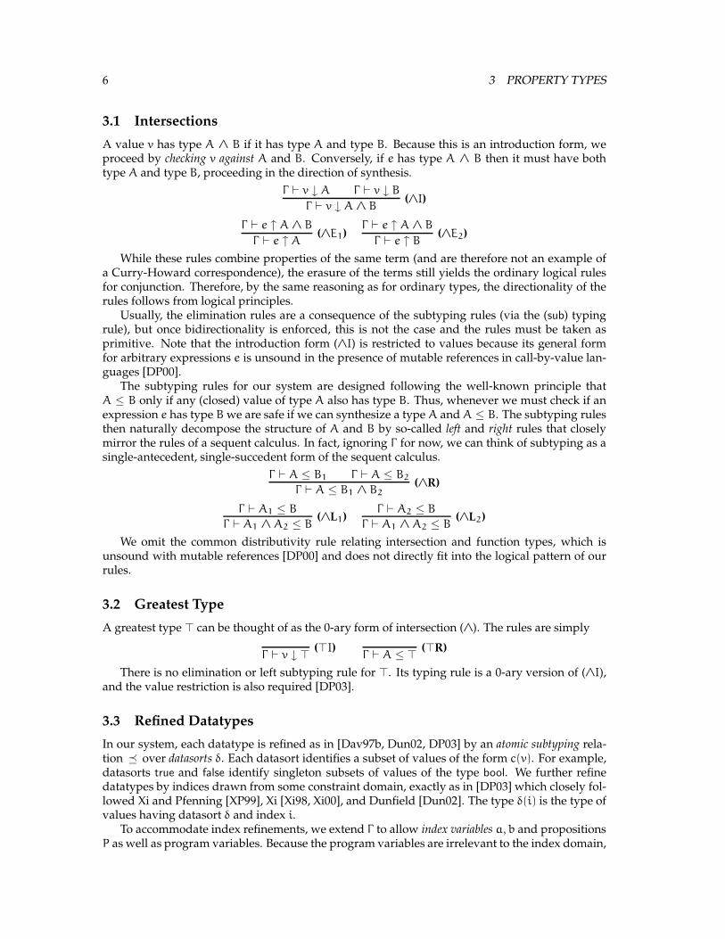
3.1 Intersections

A value v has type A ∧ B if it has type A and type B. Because this is an introduction form, weproceed by checking v against A and B. Conversely, if e has type A ∧ B then it must have bothtype A and type B, proceeding in the direction of synthesis.

Γ ` v ↓ A Γ ` v ↓ B

Γ ` v ↓ A ∧ B(∧I)

Γ ` e ↑ A ∧ B

Γ ` e ↑ A(∧E1)

Γ ` e ↑ A ∧ B

Γ ` e ↑ B(∧E2)

While these rules combine properties of the same term (and are therefore not an example ofa Curry-Howard correspondence), the erasure of the terms still yields the ordinary logical rulesfor conjunction. Therefore, by the same reasoning as for ordinary types, the directionality of therules follows from logical principles.

Usually, the elimination rules are a consequence of the subtyping rules (via the (sub) typingrule), but once bidirectionality is enforced, this is not the case and the rules must be taken asprimitive. Note that the introduction form (∧I) is restricted to values because its general formfor arbitrary expressions e is unsound in the presence of mutable references in call-by-value lan-guages [DP00].

The subtyping rules for our system are designed following the well-known principle thatA ≤ B only if any (closed) value of type A also has type B. Thus, whenever we must check if anexpression e has type B we are safe if we can synthesize a type A and A ≤ B. The subtyping rulesthen naturally decompose the structure of A and B by so-called left and right rules that closelymirror the rules of a sequent calculus. In fact, ignoring Γ for now, we can think of subtyping as asingle-antecedent, single-succedent form of the sequent calculus.

Γ ` A ≤ B1 Γ ` A ≤ B2

Γ ` A ≤ B1 ∧ B2(∧R)

Γ ` A1 ≤ B

Γ ` A1 ∧ A2 ≤ B(∧L1)

Γ ` A2 ≤ B

Γ ` A1 ∧ A2 ≤ B(∧L2)

We omit the common distributivity rule relating intersection and function types, which isunsound with mutable references [DP00] and does not directly fit into the logical pattern of ourrules.

3.2 Greatest Type

A greatest type > can be thought of as the 0-ary form of intersection (∧). The rules are simply

Γ ` v ↓ >(>I)

Γ ` A ≤ >(>R)

There is no elimination or left subtyping rule for >. Its typing rule is a 0-ary version of (∧I),and the value restriction is also required [DP03].

3.3 Refined Datatypes

In our system, each datatype is refined as in [Dav97b, Dun02, DP03] by an atomic subtyping rela-tion � over datasorts δ. Each datasort identifies a subset of values of the form c(v). For example,datasorts true and false identify singleton subsets of values of the type bool. We further refinedatatypes by indices drawn from some constraint domain, exactly as in [DP03] which closely fol-lowed Xi and Pfenning [XP99], Xi [Xi98, Xi00], and Dunfield [Dun02]. The type δ(i) is the type ofvalues having datasort δ and index i.

To accommodate index refinements, we extend Γ to allow index variables a, b and propositionsP as well as program variables. Because the program variables are irrelevant to the index domain,

3.3 Refined Datatypes 7

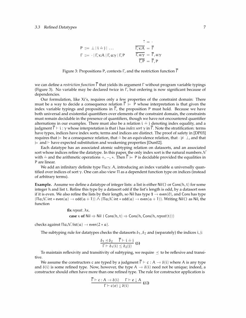
P ::= ⊥ | i.= j | . . .

Γ ::= · | Γ, x:A | Γ, a:γ | Γ, P

· = ·

Γ, x:A = Γ

Γ, a:γ = Γ , a:γ

Γ, P = Γ , P

Figure 3: Propositions P, contexts Γ , and the restriction function Γ

we can define a restriction function Γ that yields its argument Γ without program variable typings(Figure 3). No variable may be declared twice in Γ , but ordering is now significant because ofdependencies.

Our formulation, like Xi’s, requires only a few properties of the constraint domain: Theremust be a way to decide a consequence relation Γ |= P whose interpretation is that given theindex variable typings and propositions in Γ , the proposition P must hold. Because we haveboth universal and existential quantifiers over elements of the constraint domain, the constraintsmust remain decidable in the presence of quantifiers, though we have not encountered quantifieralternations in our examples. There must also be a relation i

.= j denoting index equality, and a

judgment Γ ` i : γ whose interpretation is that i has index sort γ in Γ . Note the stratification: termshave types, indices have index sorts; terms and indices are distinct. The proof of safety in [DP03]requires that |= be a consequence relation, that

.= be an equivalence relation, that · 6|= ⊥, and that

|= and ` have expected substitution and weakening properties [Dun02].

Each datatype has an associated atomic subtyping relation on datasorts, and an associatedsort whose indices refine the datatype. In this paper, the only index sort is the natural numbers Nwith

.= and the arithmetic operations +, −, ∗. Then Γ |= P is decidable provided the equalities in

P are linear.

We add an infinitary definite type Πa:γ. A, introducing an index variable a universally quan-tified over indices of sort γ. One can also view Π as a dependent function type on indices (insteadof arbitrary terms).

Example. Assume we define a datatype of integer lists: a list is either Nil() or Cons(h, t) for someinteger h and list t. Refine this type by a datasort odd if the list’s length is odd, by a datasort even

if it is even. We also refine the lists by their length, so Nil has type 1 → even(0), and Cons has type(Πa:N. int ∗ even(a) → odd(a + 1)) ∧ (Πa:N. int ∗ odd(a) → even(a + 1)). Writing Nil() as Nil, thefunction

fix repeat. λx.

case x of Nil ⇒ Nil |Cons(h, t) ⇒ Cons(h, Cons(h, repeat(t)))

checks against Πa:N. list(a) → even(2 ∗ a).

The subtyping rule for datatypes checks the datasorts δ1, δ2 and (separately) the indices i, j:

δ1 � δ2 Γ ` i.= j

Γ ` δ1(i) ≤ δ2(j)(δ)

To maintain reflexivity and transitivity of subtyping, we require � to be reflexive and transi-tive.

We assume the constructors c are typed by a judgment Γ ` c : A → δ(i) where A is any typeand δ(i) is some refined type. Now, however, the type A → δ(i) need not be unique; indeed, aconstructor should often have more than one refined type. The rule for constructor application is

Γ ` c : A → δ(i) Γ ` e ↓ A

Γ ` c(e) ↓ δ(i)(δI)

8 3 PROPERTY TYPES

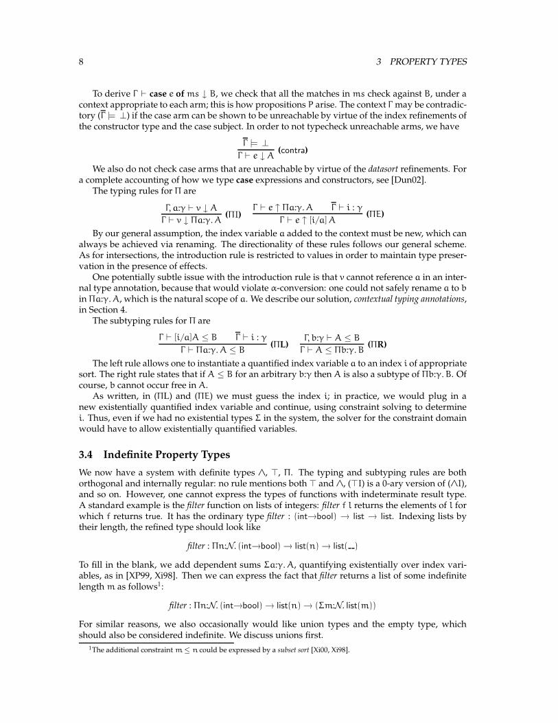
To derive Γ ` case e of ms ↓ B, we check that all the matches in ms check against B, under acontext appropriate to each arm; this is how propositions P arise. The context Γ may be contradic-tory (Γ |= ⊥) if the case arm can be shown to be unreachable by virtue of the index refinements ofthe constructor type and the case subject. In order to not typecheck unreachable arms, we have

Γ |= ⊥

Γ ` e ↓ A(contra)

We also do not check case arms that are unreachable by virtue of the datasort refinements. Fora complete accounting of how we type case expressions and constructors, see [Dun02].

The typing rules for Π are

Γ, a:γ ` v ↓ A

Γ ` v ↓ Πa:γ. A(ΠI)

Γ ` e ↑ Πa:γ. A Γ ` i : γ

Γ ` e ↑ [i/a] A(ΠE)

By our general assumption, the index variable a added to the context must be new, which canalways be achieved via renaming. The directionality of these rules follows our general scheme.As for intersections, the introduction rule is restricted to values in order to maintain type preser-vation in the presence of effects.

One potentially subtle issue with the introduction rule is that v cannot reference a in an inter-nal type annotation, because that would violate α-conversion: one could not safely rename a to b

in Πa:γ. A, which is the natural scope of a. We describe our solution, contextual typing annotations,in Section 4.

The subtyping rules for Π are

Γ ` [i/a]A ≤ B Γ ` i : γ

Γ ` Πa:γ. A ≤ B(ΠL)

Γ, b:γ ` A ≤ B

Γ ` A ≤ Πb:γ. B(ΠR)

The left rule allows one to instantiate a quantified index variable a to an index i of appropriatesort. The right rule states that if A ≤ B for an arbitrary b:γ then A is also a subtype of Πb:γ. B. Ofcourse, b cannot occur free in A.

As written, in (ΠL) and (ΠE) we must guess the index i; in practice, we would plug in anew existentially quantified index variable and continue, using constraint solving to determinei. Thus, even if we had no existential types Σ in the system, the solver for the constraint domainwould have to allow existentially quantified variables.

3.4 Indefinite Property Types

We now have a system with definite types ∧, >, Π. The typing and subtyping rules are bothorthogonal and internally regular: no rule mentions both > and ∧, (>I) is a 0-ary version of (∧I),and so on. However, one cannot express the types of functions with indeterminate result type.A standard example is the filter function on lists of integers: filter f l returns the elements of l forwhich f returns true. It has the ordinary type filter : (int→bool) → list → list. Indexing lists bytheir length, the refined type should look like

filter : Πn:N. (int→bool) → list(n) → list( )

To fill in the blank, we add dependent sums Σa:γ. A, quantifying existentially over index vari-ables, as in [XP99, Xi98]. Then we can express the fact that filter returns a list of some indefinitelength m as follows1:

filter : Πn:N. (int→bool) → list(n) → (Σm:N. list(m))

For similar reasons, we also occasionally would like union types and the empty type, whichshould also be considered indefinite. We discuss unions first.

1The additional constraint m≤ n could be expressed by a subset sort [Xi00, Xi98].

3.4 Indefinite Property Types 9

On values, the binary indefinite type is simply a union in the ordinary sense: if v : A ∨ B

then either v : A or v : B. The introduction rules directly express the simple logical interpretation,again using checking for the introduction form.

Γ ` e ↓ A

Γ ` e ↓ A ∨ B(∨I1)

Γ ` e ↓ B

Γ ` e ↓ A ∨ B(∨I2)

No restriction to values is needed for the introductions, but, dually to intersections, the elim-ination must be restricted. A sound formulation of the elimination rule in a type assignmentform [DP03] without a syntactic marker2 requires an evaluation context E around the subterm ofunion type.

Γ ` e ′ : A ∨ B

Γ, x:A ` E[x] : C

Γ, y:B ` E[y] : C

Γ ` E[e ′] : C

This is where the “third direction” is necessary. We no longer move from terms to their imme-diate subterms, but when typechecking e we may have to decompose it into an evaluation contextE and subterm e ′. Using the analysis and synthesis judgments we have

Γ ` e ′ ↑ A ∨ B

Γ, x:A ` E[x] ↓ C

Γ, y:B ` E[y] ↓ C

Γ ` E[e ′] ↓ C(∨E)

Here, if we can synthesize a union type for e ′—which is in evaluation position in E[e ′]—andcheck E[x] and E[y] against C, assuming that x and y have type A and type B respectively, wecan conclude that E[e ′] checks against C. Note that the assumptions x:A and y:B can be read asx↑A and y↑B so we do indeed transition from ↑ A ∨ B to ↑ A and ↑ B. While typecheckingstill somehow follows the syntax, there may be many choices of E and e ′, leading to excessivenondeterminism.

The subtyping rules are standard and dual to the intersection rules.

Γ ` A1 ≤ B Γ ` A2 ≤ B

Γ ` A1 ∨ A2 ≤ B(∨L)

Γ ` A ≤ B1

Γ ` A ≤ B1 ∨ B2(∨R1)

Γ ` A ≤ B2

Γ ` A ≤ B1 ∨ B2(∨R2)

The 0-ary indefinite type is the empty or void type ⊥; it has no values and therefore no intro-duction rules. For an elimination rule (⊥E), we proceed by analogy with (∨E):

Γ ` e ′ ↑ ⊥

Γ ` E[e ′] ↓ C(⊥E)

As before, the expression must be an evaluation context E with e ′ in evaluation position. For >we had one right subtyping rule; for ⊥, following the principle of duality, we have one left rule:

Γ ` ⊥ ≤ A(⊥L)

For existential dependent types, the introduction rule presents no difficulties, and proceedsusing the analysis judgment.

Γ ` e ↓ [i/a] A Γ ` i : γ

Γ ` e ↓ Σa:γ. A(ΣI)

For the elimination rule, we follow (∨E) and (⊥E):

2Pierce [Pie91b] used an explicit marker case e′ of x ⇒ e as the union elimination form. This is technically straight-forward but a heavy burden on the programmer, particularly as markers would also be needed to eliminate Σ types,which are especially common in code without refinements; legacy code would have to be extensively “marked” to makeit typecheck.

10 3 PROPERTY TYPES

Γ ` B1 ≤ A1 Γ ` A2 ≤ B2

Γ ` A1 → A2 ≤ B1 → B2(→)

Γ ` 1 ≤ 1(1)

Γ ` A1 ≤ B1 Γ ` A2 ≤ B2

Γ ` A1 ∗ A2 ≤ B1 ∗ B2(∗)

Γ ` A ≤ B1 Γ ` A ≤ B2

Γ ` A ≤ B1 ∧ B2(∧R)

Γ ` A1 ≤ B

Γ ` A1 ∧ A2 ≤ B(∧L1)

Γ ` A2 ≤ B

Γ ` A1 ∧ A2 ≤ B(∧L2)

δ1 � δ2 Γ ` i.= j

Γ ` δ1(i) ≤ δ2(j)(δ)

Γ ` [i/a]A ≤ B Γ ` i : γ

Γ ` Πa:γ. A ≤ B(ΠL)

Γ, b:γ ` A ≤ B

Γ ` A ≤ Πb:γ. B(ΠR)

Γ ` A1 ≤ B Γ ` A2 ≤ B

Γ ` A1 ∨ A2 ≤ B(∨L)

Γ ` A ≤ B1

Γ ` A ≤ B1 ∨ B2(∨R1)

Γ ` A ≤ B2

Γ ` A ≤ B1 ∨ B2(∨R2)

Γ ` ⊥ ≤ A(⊥L)

Γ ` A ≤ >(>R)

Γ, a:γ ` A ≤ B

Γ ` Σa:γ. A ≤ B(ΣL)

Γ ` A ≤ [i/b] B Γ ` i : γ

Γ ` A ≤ Σb:γ. B(ΣR)

Figure 4: Subtyping in the full language

Γ ` e ′ ↑ Σa:γ. A Γ, a:γ, x:A ` E[x] ↓ C

Γ ` E[e ′] ↓ C(ΣE)

Again, there is a potentially subtle issue: the index variable a must be new and cannot bementioned in an annotation in E.

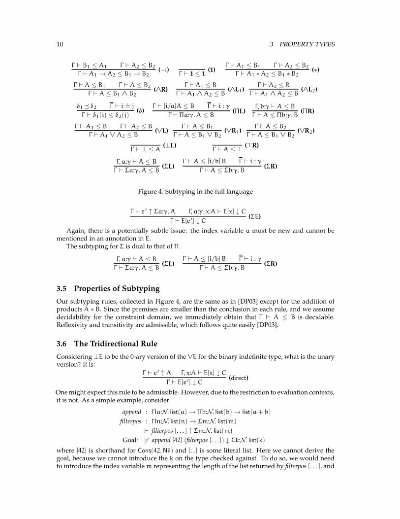
The subtyping for Σ is dual to that of Π.

Γ, a:γ ` A ≤ B

Γ ` Σa:γ. A ≤ B(ΣL)

Γ ` A ≤ [i/b] B Γ ` i : γ

Γ ` A ≤ Σb:γ. B(ΣR)

3.5 Properties of Subtyping

Our subtyping rules, collected in Figure 4, are the same as in [DP03] except for the addition ofproducts A ∗ B. Since the premises are smaller than the conclusion in each rule, and we assumedecidability for the constraint domain, we immediately obtain that Γ ` A ≤ B is decidable.Reflexivity and transitivity are admissible, which follows quite easily [DP03].

3.6 The Tridirectional Rule

Considering ⊥E to be the 0-ary version of the ∨E for the binary indefinite type, what is the unaryversion? It is:

Γ ` e ′ ↑ A Γ, x:A ` E[x] ↓ C

Γ ` E[e ′] ↓ C(direct)

One might expect this rule to be admissible. However, due to the restriction to evaluation contexts,it is not. As a simple example, consider

append : Πa:N. list(a) → Πb:N. list(b) → list(a + b)

filterpos : Πn:N. list(n) → Σm:N. list(m)

` filterpos [. . . ] ↑ Σm:N. list(m)

Goal: 6` append [42] (filterpos [. . . ]) ↓ Σk:N. list(k)

where [42] is shorthand for Cons(42, Nil) and [...] is some literal list. Here we cannot derive thegoal, because we cannot introduce the k on the type checked against. To do so, we would needto introduce the index variable m representing the length of the list returned by filterpos [. . . ], and

11

use m + 1 for k. But filterpos [. . . ] is not in evaluation position, because append [42] will need to beevaluated first. However, append [42] synthesizes only type Πb:N. list(b) → list(1 + b), so we arestuck. However, using rule (direct) we reduce

append [42] (filterpos [. . . ]) ↓ Σk:N. list(k)

tox : Πb:N. list(b)→list(1+b) ` x (filterpos [. . . ]) ↓ Σk:N. list(k)

Since x is a value, (filterpos [. . .]) is in evaluation position and we can use the existential eliminationrule

x:Πb:N. list(b)→list(1+b), m:N, y:list(m) ` x y ↓ Σk:N. list(k)

Now we can complete the derivation with (ΣI), using 1 + m for k and several straightforwardsteps.

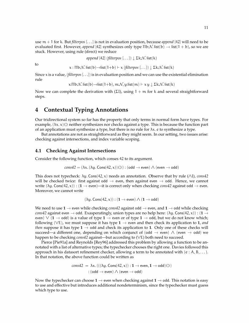
4 Contextual Typing Annotations

Our tridirectional system so far has the property that only terms in normal form have types. Forexample, (λx. x)() neither synthesizes nor checks against a type. This is because the function partof an application must synthesize a type, but there is no rule for λx. e to synthesize a type.

But annotations are not as straightforward as they might seem. In our setting, two issues arise:checking against intersections, and index variable scoping.

4.1 Checking Against Intersections

Consider the following function, which conses 42 to its argument.

cons42 = (λx. (λy. Cons(42, x))()) : (odd → even) ∧ (even → odd)

This does not typecheck: λy. Cons(42, x) needs an annotation. Observe that by rule (∧I), cons42will be checked twice: first against odd → even, then against even → odd. Hence, we cannotwrite (λy. Cons(42, x)) : (1 → even)—it is correct only when checking cons42 against odd → even.Moreover, we cannot write

(λy. Cons(42, x)) : (1 → even) ∧ (1 → odd)

We need to use 1 → even while checking cons42 against odd → even, and 1 → odd while checkingcons42 against even → odd. Exasperatingly, union types are no help here: (λy. Cons(42, x)) : (1 →

even) ∨ (1 → odd) is a value of type 1 → even or of type 1 → odd, but we do not know which;following (∨E), we must suppose it has type 1 → even and then check its application to 1, andthen suppose it has type 1 → odd and check its application to 1. Only one of these checks willsucceed—a different one, depending on which conjunct of (odd → even) ∧ (even → odd) wehappen to be checking cons42 against—but according to (∨E) both need to succeed.

Pierce [Pie91a] and Reynolds [Rey96] addressed this problem by allowing a function to be an-notated with a list of alternative types; the typechecker chooses the right one. Davies followed thisapproach in his datasort refinement checker, allowing a term to be annotated with (e : A, B, . . . ).In that notation, the above function could be written as

cons42 = λx. (((λy. Cons(42, x)) : 1 → even, 1 → odd)())

: (odd → even) ∧ (even → odd)

Now the typechecker can choose 1 → even when checking against 1 → odd. This notation is easyto use and effective but introduces additional nondeterminism, since the typechecker must guesswhich type to use.

12 4 CONTEXTUAL TYPING ANNOTATIONS

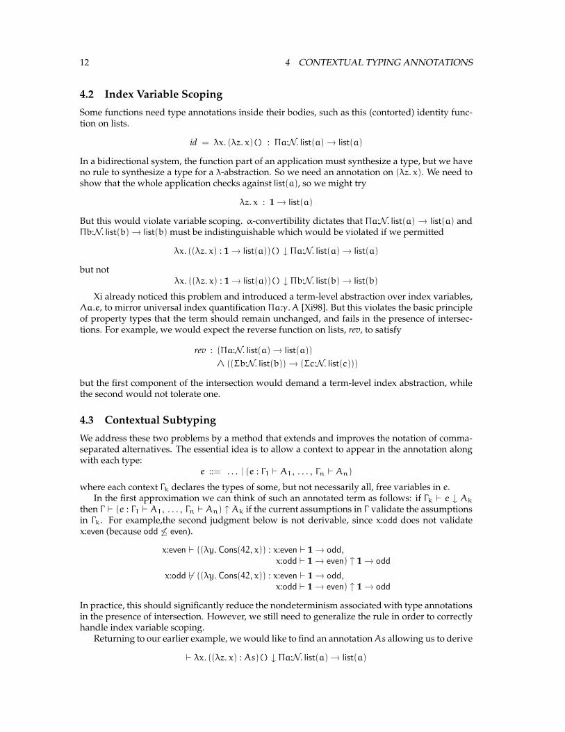
4.2 Index Variable Scoping

Some functions need type annotations inside their bodies, such as this (contorted) identity func-tion on lists.

id = λx. (λz. x)() : Πa:N. list(a) → list(a)

In a bidirectional system, the function part of an application must synthesize a type, but we haveno rule to synthesize a type for a λ-abstraction. So we need an annotation on (λz. x). We need toshow that the whole application checks against list(a), so we might try

λz. x : 1 → list(a)

But this would violate variable scoping. α-convertibility dictates that Πa:N. list(a) → list(a) andΠb:N. list(b) → list(b) must be indistinguishable which would be violated if we permitted

λx. ((λz. x) : 1 → list(a))() ↓ Πa:N. list(a) → list(a)

but notλx. ((λz. x) : 1 → list(a))() ↓ Πb:N. list(b) → list(b)

Xi already noticed this problem and introduced a term-level abstraction over index variables,Λa.e, to mirror universal index quantification Πa:γ. A [Xi98]. But this violates the basic principleof property types that the term should remain unchanged, and fails in the presence of intersec-tions. For example, we would expect the reverse function on lists, rev, to satisfy

rev : (Πa:N. list(a) → list(a))

∧ ((Σb:N. list(b)) → (Σc:N. list(c)))

but the first component of the intersection would demand a term-level index abstraction, whilethe second would not tolerate one.

4.3 Contextual Subtyping

We address these two problems by a method that extends and improves the notation of comma-separated alternatives. The essential idea is to allow a context to appear in the annotation alongwith each type:

e ::= . . . | (e : Γ1 ` A1, . . . , Γn ` An)

where each context Γk declares the types of some, but not necessarily all, free variables in e.In the first approximation we can think of such an annotated term as follows: if Γk ` e ↓ Ak

then Γ ` (e : Γ1 ` A1, . . . , Γn ` An) ↑ Ak if the current assumptions in Γ validate the assumptionsin Γk. For example,the second judgment below is not derivable, since x:odd does not validatex:even (because odd 6≤ even).

x:even ` ((λy. Cons(42, x)) : x:even ` 1 → odd,

x:odd ` 1 → even) ↑ 1 → odd

x:odd 6` ((λy. Cons(42, x)) : x:even ` 1 → odd,

x:odd ` 1 → even) ↑ 1 → odd

In practice, this should significantly reduce the nondeterminism associated with type annotationsin the presence of intersection. However, we still need to generalize the rule in order to correctlyhandle index variable scoping.

Returning to our earlier example, we would like to find an annotation As allowing us to derive

` λx. ((λz. x) : As)() ↓ Πa:N. list(a) → list(a)

4.3 Contextual Subtyping 13

The idea is to use a locally declared index variable (here, b)

λx. ((λz. x) : (b:N, x:list(b) ` 1 → list(b)))

to make the typing annotation self-contained. Now, when we check if the current assumptionsfor x validate local assumption for x, we are permitted to instantiate b to any index object i. Inthis example, we could substitute a for b. As a result, we end up checking (λz. x) ↓ 1 → list(a),even though the annotation does not mention a. Note that in an annotation e : (Γ0 ` A0), As, allindex variables declared in Γ0 are considered bound and can be renamed consistently in Γ0 andA0. In contrast, the free term variables in Γ0 may actually occur in e and so cannot be renamedfreely.

These considerations lead to a contextual subtyping relation . :

(Γ0 ` A0) . (Γ ` A)

which is contravariant in the contexts Γ0 and Γ . It would be covariant in A0 and A, except thatin the way it is invoked, Γ0, A0, and Γ are known and A is generated as an instance of A0. Thisshould become more clear when we consider its use in the new typing rule

(Γ0 ` A0) . (Γ ` A) Γ ` e ↓ A

Γ ` (e : (Γ0 ` A0), As) ↑ A(ctx-anno)

where we regard the annotations as unordered (so Γ0 ` A0 could occur anywhere in the list).In the bidirectional style, Γ , e, Γ0, A0 and As are known when we try this rule. While finding aderivation of (Γ0 ` A0) . (Γ ` A) we generate A, which is the synthesized type of the originalannotated expression e, if in fact e checks against A. It is also possible that (Γ0 ` A0) . (Γ ` A)

fails to have a derivation (when Γ0 and Γ have incompatible declarations for the term variablesoccurring in them), in which case we need to try another annotation (Γk ` Ak).

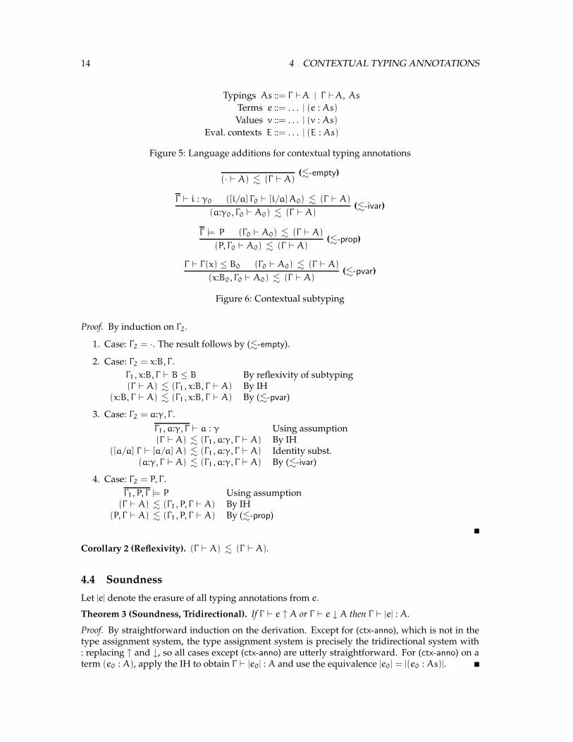
The formal rules for contextual subtyping are given in Figure 6. Besides the considerationsabove, we also must make sure that any possible assumptions P about the index variables in Γ0

are indeed entailed by the current context, after any possible substitution has been applied (thisis why we traverse Γ0 from left to right).

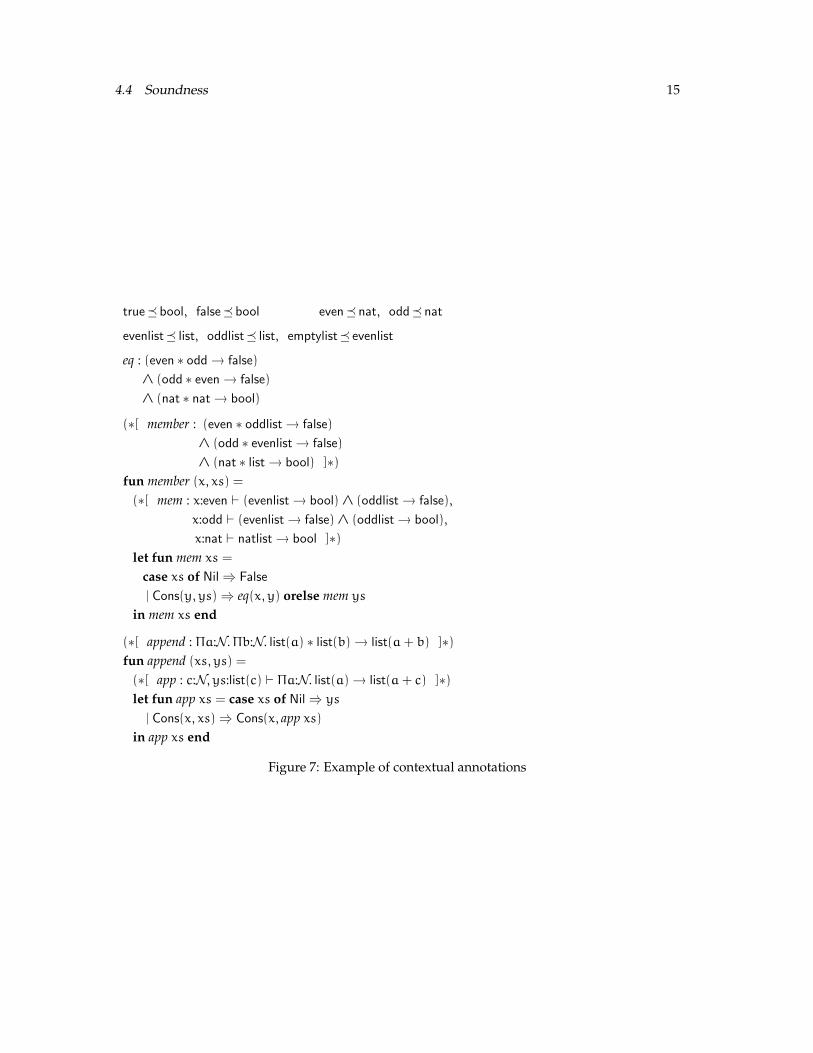
While the examples above are artificial, similar situations arise in ordinary programs in thecommon situation when local function definitions reference free variables. Two small examplesof this kind are given in Figure 7, presented in the style of ML, where we have omitted the ev-ident constructor types and, following the tradition of systems such as Davies’, written typingannotations inside bracketed comments.

The essence of the completeness result we prove in Section 4.5 is that annotations can be addedto any term that is well typed in the type assignment system to yield a well typed term in the tridi-rectional system. For this result to hold, . must be reflexive, (Γ ` A) . (Γ ` A). Furthermore,in a judgment

Γ ` (e : (Γ1 ` A1, . . . , Γn ` An)) ↑ A

we must be able to consistently rename index variables in Γ , all Γk, and e. This different treatmentof index variables and term variables arises from the fact that index variables are associated withproperty types and so do not appear in expressions, only in types.

Reflexivity (together with proper α-conversion) is sufficient for completeness: in the proofof completeness, where we see Γ ` e : A we can simply add an annotation (Γ ` A). But itwould be absurd to make programmers type in entire contexts—not only is the length impractical,but whenever a declaration is added every contextual annotation in its scope would have to bechanged!

Reflexivity of . follows easily from the following lemma.

Lemma 1. (Γ2 ` A) . (Γ1, Γ2 ` A).

14 4 CONTEXTUAL TYPING ANNOTATIONS

Typings As ::= Γ `A | Γ `A, As

Terms e ::= . . . | (e : As)

Values v ::= . . . | (v : As)

Eval. contexts E ::= . . . | (E : As)

Figure 5: Language additions for contextual typing annotations

(· ` A) . (Γ ` A)(.-empty)

Γ ` i : γ0 ([i/a] Γ0 ` [i/a] A0) . (Γ ` A)

(a:γ0, Γ0 ` A0) . (Γ ` A)(.-ivar)

Γ |= P (Γ0 ` A0) . (Γ ` A)

(P, Γ0 ` A0) . (Γ ` A)(.-prop)

Γ ` Γ(x) ≤ B0 (Γ0 ` A0) . (Γ ` A)

(x:B0, Γ0 ` A0) . (Γ ` A)(.-pvar)

Figure 6: Contextual subtyping

Proof. By induction on Γ2.

1. Case: Γ2 = ·. The result follows by (.-empty).

2. Case: Γ2 = x:B, Γ .

Γ1, x:B, Γ ` B ≤ B By reflexivity of subtyping(Γ ` A) . (Γ1, x:B, Γ ` A) By IH

(x:B, Γ ` A) . (Γ1, x:B, Γ ` A) By (.-pvar)

3. Case: Γ2 = a:γ, Γ .

Γ1, a:γ, Γ ` a : γ Using assumption(Γ ` A) . (Γ1, a:γ, Γ ` A) By IH

([a/a] Γ ` [a/a] A) . (Γ1, a:γ, Γ ` A) Identity subst.(a:γ, Γ ` A) . (Γ1, a:γ, Γ ` A) By (.-ivar)

4. Case: Γ2 = P, Γ .

Γ1, P, Γ |= P Using assumption(Γ ` A) . (Γ1, P, Γ ` A) By IH

(P, Γ ` A) . (Γ1, P, Γ ` A) By (.-prop)

Corollary 2 (Reflexivity). (Γ ` A) . (Γ ` A).

4.4 Soundness

Let |e| denote the erasure of all typing annotations from e.

Theorem 3 (Soundness, Tridirectional). If Γ ` e ↑ A or Γ ` e ↓ A then Γ ` |e| : A.

Proof. By straightforward induction on the derivation. Except for (ctx-anno), which is not in thetype assignment system, the type assignment system is precisely the tridirectional system with: replacing ↑ and ↓, so all cases except (ctx-anno) are utterly straightforward. For (ctx-anno) on aterm (e0 : A), apply the IH to obtain Γ ` |e0| : A and use the equivalence |e0| = |(e0 : As)|.

4.4 Soundness 15

true� bool, false� bool even� nat, odd� nat

evenlist� list, oddlist� list, emptylist� evenlist

eq : (even ∗ odd → false)

∧ (odd ∗ even → false)

∧ (nat ∗ nat → bool)

(∗[ member : (even ∗ oddlist → false)

∧ (odd ∗ evenlist → false)

∧ (nat ∗ list → bool) ]∗)

fun member (x, xs) =

(∗[ mem : x:even ` (evenlist → bool) ∧ (oddlist → false),

x:odd ` (evenlist → false) ∧ (oddlist → bool),

x:nat ` natlist → bool ]∗)

let fun mem xs =

case xs of Nil ⇒ False

| Cons(y, ys) ⇒ eq(x, y) orelse mem ys

in mem xs end

(∗[ append : Πa:N. Πb:N. list(a) ∗ list(b) → list(a + b) ]∗)

fun append (xs, ys) =

(∗[ app : c:N, ys:list(c) ` Πa:N. list(a) → list(a + c) ]∗)

let fun app xs = case xs of Nil ⇒ ys

| Cons(x, xs) ⇒ Cons(x, app xs)

in app xs end

Figure 7: Example of contextual annotations

16 4 CONTEXTUAL TYPING ANNOTATIONS

4.5 Completeness

We cannot just take a derivation Γ ` e : A in the type assignment system and obtain a derivationΓ ` e ↑ A in the tridirectional system. For example, ` λx. x : A → A for any type A, but in thetridirectional system λx. x does not synthesize a type. However, if we add a typing annotation,we can derive

` (λx. x : (` A → A)) ↑ A → A

Clearly, the completeness result must be along the lines of “If Γ ` e : A, then there is an annotatedversion e ′ of e such that Γ ` e ′ ↑ A.” To formulate this result (Corollary 15, a special case ofTheorem 14) we need a few definitions and lemmas.

Definition 4. A term is in synthesizing form if it has any of the forms

x, e1e2, u, (e : As), fst(e), snd(e)

Proposition 5. If Γ ` e ↑ A then e is in synthesizing form.

Proof. By induction on the derivation.

Remark 1. The point of a type annotation is to obtain a synthesizing term from a non-synthesizingone. It is never necessary to add a typing annotation to the root of a term in synthesizing form(though annotations may be needed inside the term).

Definition 6. e ′ extends a term e, written e ′ w e iff e ′ is e with zero or more additional typing annota-tions and e ′ contains no type annotations on the roots of terms in synthesizing form.

Definition 7. e ′ lightly extends a term e, written e ′ w` e iff e ′ is e with zero or more typing annotationsadded to lists of typing annotations already present in e. That is, we can replace (e : As) with (e :

As, A ′), but cannot replace e with (e : A ′).

Proposition 8. w and w` are reflexive and transitive.

Proof. Obvious from the definitions.

Lemma 9. If e value and e ′ w e then e ′ value.

Proof. By a straightforward induction on e ′ (making use of (v : As) value).

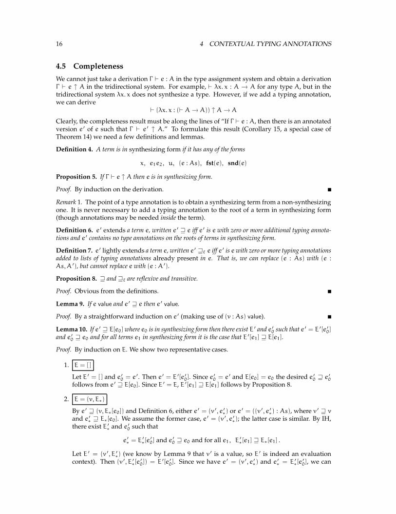
Lemma 10. If e ′ w E[e0] where e0 is in synthesizing form then there exist E ′ and e ′

0 such that e ′ = E ′[e ′

0]

and e ′

0 w e0 and for all terms e1 in synthesizing form it is the case that E ′[e1] w E[e1].

Proof. By induction on E. We show two representative cases.

1. E = [ ]

Let E ′ = [ ] and e ′

0 = e ′. Then e ′ = E ′[e ′

0]. Since e ′

0 = e ′ and E[e0] = e0 the desired e ′

0 w e ′

0

follows from e ′ w E[e0]. Since E ′ = E, E ′[e1] w E[e1] follows by Proposition 8.

2. E = (v, E∗)

By e ′ w (v, E∗[e0]) and Definition 6, either e ′ = (v ′, e ′

∗) or e ′ = ((v ′, e ′

∗) : As), where v ′ w v

and e ′

∗w E∗[e0]. We assume the former case, e ′ = (v ′, e ′

∗); the latter case is similar. By IH,

there exist E ′

∗and e ′

0 such that

e ′

∗= E ′

∗[e ′

0] and e ′

0 w e0 and for all e1, E ′

∗[e1] w E∗[e1] .

Let E ′ = (v ′, E ′

∗) (we know by Lemma 9 that v ′ is a value, so E ′ is indeed an evaluation

context). Then (v ′, E ′

∗[e ′

0]) = E ′[e ′

0]. Since we have e ′ = (v ′, e ′

∗) and e ′

∗= E ′

∗[e ′

0], we can

4.5 Completeness 17

conclude e ′ = E ′[E ′

0], the first part of what was to be shown. The second part, e ′

0 w e0, wealready know by IH. Now take any e1. We know v ′ w v and by IH we have E ′

∗[e1] w E∗[e1].

Therefore (v ′, E ′

∗[e1]) w (v, E∗[e1]). By E ′[e1] = (v ′, E ′

∗[e1]) and (v, E∗[e1]) = E[e1],

E ′[e1] w E[e1]

which is the last part of what was to be shown.

Lemma 11. If e ′ w` E[e0] where e0 is in synthesizing form then there exist E ′ and e ′

0 such that e ′ =

E ′[e ′

0] and e ′

0 w` e0 and for all e1 in synthesizing form it is the case that E ′[e1] w` E[e1].

Proof. By induction on E, following the proof of Lemma 10.

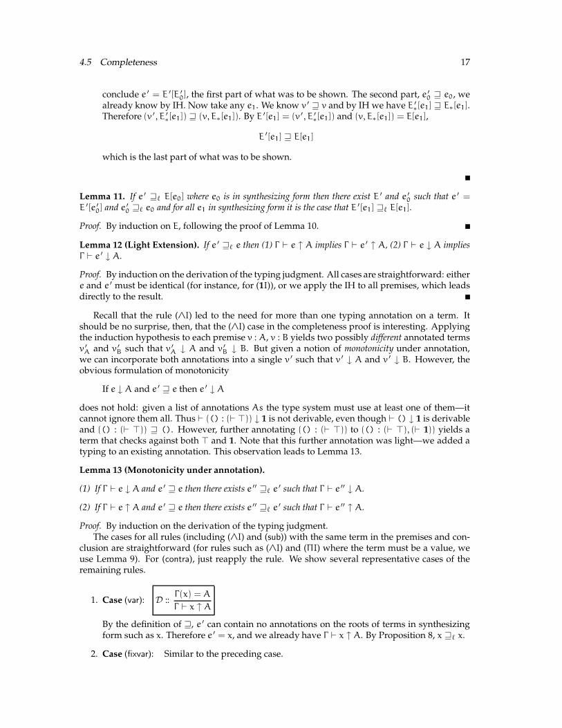
Lemma 12 (Light Extension). If e ′ w` e then (1) Γ ` e ↑ A implies Γ ` e ′ ↑ A, (2) Γ ` e ↓ A impliesΓ ` e ′ ↓ A.

Proof. By induction on the derivation of the typing judgment. All cases are straightforward: eithere and e ′ must be identical (for instance, for (1I)), or we apply the IH to all premises, which leadsdirectly to the result.

Recall that the rule (∧I) led to the need for more than one typing annotation on a term. Itshould be no surprise, then, that the (∧I) case in the completeness proof is interesting. Applyingthe induction hypothesis to each premise v : A, v : B yields two possibly different annotated termsv ′

A and v ′

B such that v ′

A ↓ A and v ′

B ↓ B. But given a notion of monotonicity under annotation,we can incorporate both annotations into a single v ′ such that v ′ ↓ A and v ′ ↓ B. However, theobvious formulation of monotonicity

If e ↓ A and e ′ w e then e ′ ↓ A

does not hold: given a list of annotations As the type system must use at least one of them—itcannot ignore them all. Thus ` (() : (` >)) ↓ 1 is not derivable, even though ` () ↓ 1 is derivableand (() : (` >)) w (). However, further annotating (() : (` >)) to (() : (` >), (` 1)) yields aterm that checks against both > and 1. Note that this further annotation was light—we added atyping to an existing annotation. This observation leads to Lemma 13.

Lemma 13 (Monotonicity under annotation).

(1) If Γ ` e ↓ A and e ′ w e then there exists e ′′ w` e ′ such that Γ ` e ′′ ↓ A.

(2) If Γ ` e ↑ A and e ′ w e then there exists e ′′ w` e ′ such that Γ ` e ′′ ↑ A.

Proof. By induction on the derivation of the typing judgment.The cases for all rules (including (∧I) and (sub)) with the same term in the premises and con-

clusion are straightforward (for rules such as (∧I) and (ΠI) where the term must be a value, weuse Lemma 9). For (contra), just reapply the rule. We show several representative cases of theremaining rules.

1. Case (var): D ::Γ(x) = A

Γ ` x ↑ A

By the definition of w, e ′ can contain no annotations on the roots of terms in synthesizingform such as x. Therefore e ′ = x, and we already have Γ ` x ↑ A. By Proposition 8, x w` x.

2. Case (fixvar): Similar to the preceding case.

18 4 CONTEXTUAL TYPING ANNOTATIONS

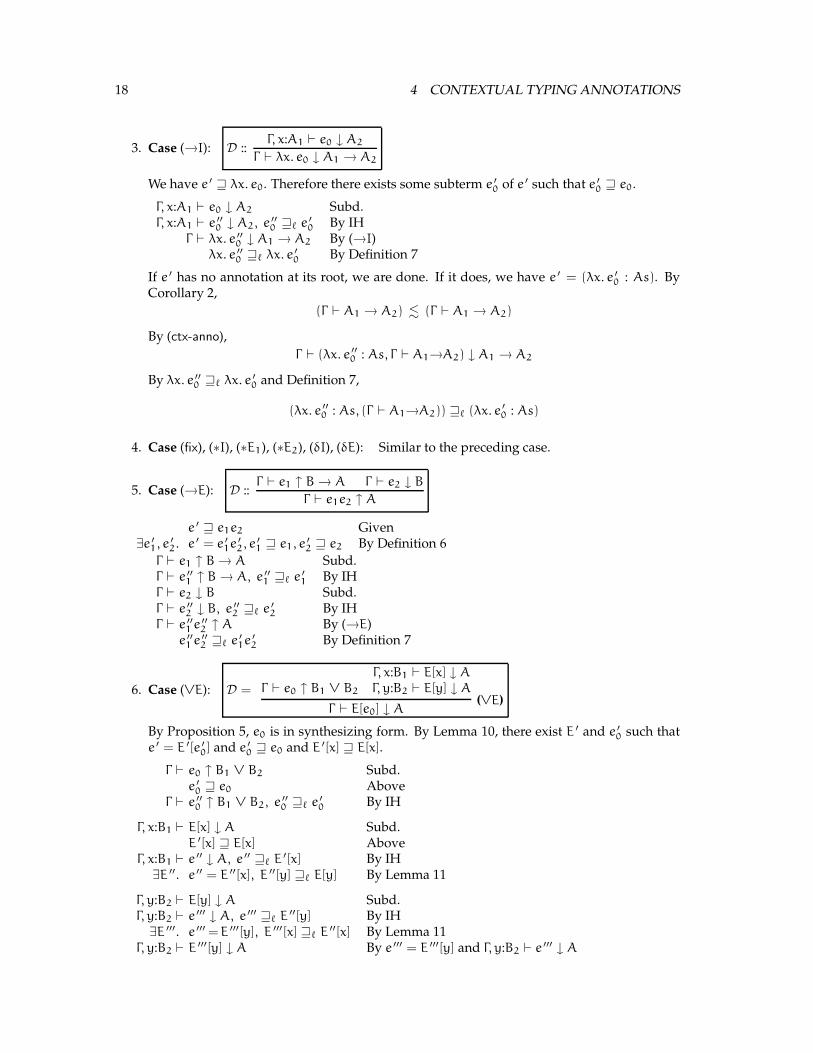
3. Case (→I): D ::Γ, x:A1 ` e0 ↓ A2

Γ ` λx. e0 ↓ A1 → A2

We have e ′ w λx. e0. Therefore there exists some subterm e ′

0 of e ′ such that e ′

0 w e0.

Γ, x:A1 ` e0 ↓ A2 Subd.Γ, x:A1 ` e ′′

0 ↓ A2, e ′′

0 w` e ′

0 By IHΓ ` λx. e ′′

0 ↓ A1 → A2 By (→I)λx. e ′′

0 w` λx. e ′

0 By Definition 7

If e ′ has no annotation at its root, we are done. If it does, we have e ′ = (λx. e ′

0 : As). ByCorollary 2,

(Γ ` A1 → A2) . (Γ ` A1 → A2)

By (ctx-anno),

Γ ` (λx. e ′′

0 : As, Γ ` A1→A2) ↓ A1 → A2

By λx. e ′′

0 w` λx. e ′

0 and Definition 7,

(λx. e ′′

0 : As, (Γ ` A1→A2)) w` (λx. e ′

0 : As)

4. Case (fix), (∗I), (∗E1), (∗E2), (δI), (δE): Similar to the preceding case.

5. Case (→E): D ::Γ ` e1 ↑ B → A Γ ` e2 ↓ B

Γ ` e1e2 ↑ A

e ′ w e1e2 Given∃e ′

1, e ′

2. e ′ = e ′

1e ′

2, e ′

1 w e1, e ′

2 w e2 By Definition 6

Γ ` e1 ↑ B → A Subd.Γ ` e ′′

1 ↑ B → A, e ′′

1 w` e ′

1 By IHΓ ` e2 ↓ B Subd.Γ ` e ′′

2 ↓ B, e ′′

2 w` e ′

2 By IHΓ ` e ′′

1 e ′′

2 ↑ A By (→E)e ′′

1 e ′′

2 w` e ′

1e ′

2 By Definition 7

6. Case (∨E): D = Γ ` e0 ↑ B1 ∨ B2

Γ, x:B1 ` E[x] ↓ A

Γ, y:B2 ` E[y] ↓ A

Γ ` E[e0] ↓ A(∨E)

By Proposition 5, e0 is in synthesizing form. By Lemma 10, there exist E ′ and e ′

0 such thate ′ = E ′[e ′

0] and e ′

0 w e0 and E ′[x] w E[x].

Γ ` e0 ↑ B1 ∨ B2 Subd.e ′

0 w e0 AboveΓ ` e ′′

0 ↑ B1 ∨ B2, e ′′

0 w` e ′

0 By IH

Γ, x:B1 ` E[x] ↓ A Subd.E ′[x] w E[x] Above

Γ, x:B1 ` e ′′ ↓ A, e ′′ w` E ′[x] By IH∃E ′′. e ′′ = E ′′[x], E ′′[y] w` E[y] By Lemma 11

Γ, y:B2 ` E[y] ↓ A Subd.Γ, y:B2 ` e ′′′ ↓ A, e ′′′ w` E ′′[y] By IH∃E ′′′. e ′′′ = E ′′′[y], E ′′′[x] w` E ′′[x] By Lemma 11

Γ, y:B2 ` E ′′′[y] ↓ A By e ′′′ = E ′′′[y] and Γ, y:B2 ` e ′′′ ↓ A

4.5 Completeness 19

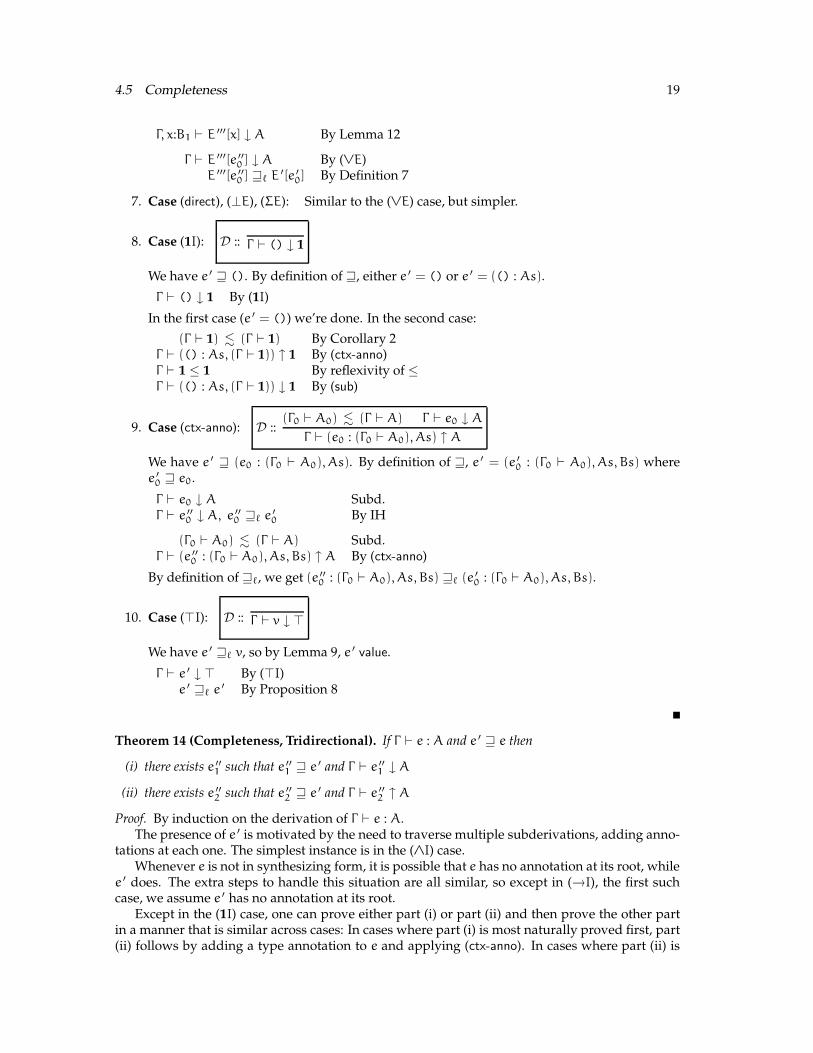
Γ, x:B1 ` E ′′′[x] ↓ A By Lemma 12

Γ ` E ′′′[e ′′

0 ] ↓ A By (∨E)E ′′′[e ′′

0 ] w` E ′[e ′

0] By Definition 7

7. Case (direct), (⊥E), (ΣE): Similar to the (∨E) case, but simpler.

8. Case (1I): D :: Γ ` () ↓ 1

We have e ′ w (). By definition of w, either e ′ = () or e ′ = (() : As).

Γ ` () ↓ 1 By (1I)

In the first case (e ′ = ()) we’re done. In the second case:

(Γ ` 1) . (Γ ` 1) By Corollary 2Γ ` (() : As, (Γ ` 1)) ↑ 1 By (ctx-anno)Γ ` 1 ≤ 1 By reflexivity of ≤Γ ` (() : As, (Γ ` 1)) ↓ 1 By (sub)

9. Case (ctx-anno): D ::(Γ0 ` A0) . (Γ ` A) Γ ` e0 ↓ A

Γ ` (e0 : (Γ0 ` A0), As) ↑ A

We have e ′ w (e0 : (Γ0 ` A0), As). By definition of w, e ′ = (e ′

0 : (Γ0 ` A0), As, Bs) wheree ′

0 w e0.

Γ ` e0 ↓ A Subd.Γ ` e ′′

0 ↓ A, e ′′

0 w` e ′

0 By IH

(Γ0 ` A0) . (Γ ` A) Subd.Γ ` (e ′′

0 : (Γ0 ` A0), As, Bs) ↑ A By (ctx-anno)

By definition of w`, we get (e ′′

0 : (Γ0 ` A0), As, Bs) w` (e ′

0 : (Γ0 ` A0), As, Bs).

10. Case (>I): D :: Γ ` v ↓ >

We have e ′ w` v, so by Lemma 9, e ′ value.

Γ ` e ′ ↓ > By (>I)e ′ w` e ′ By Proposition 8

Theorem 14 (Completeness, Tridirectional). If Γ ` e : A and e ′ w e then

(i) there exists e ′′

1 such that e ′′

1 w e ′ and Γ ` e ′′

1 ↓ A

(ii) there exists e ′′

2 such that e ′′

2 w e ′ and Γ ` e ′′

2 ↑ A

Proof. By induction on the derivation of Γ ` e : A.The presence of e ′ is motivated by the need to traverse multiple subderivations, adding anno-

tations at each one. The simplest instance is in the (∧I) case.Whenever e is not in synthesizing form, it is possible that e has no annotation at its root, while

e ′ does. The extra steps to handle this situation are all similar, so except in (→I), the first suchcase, we assume e ′ has no annotation at its root.

Except in the (1I) case, one can prove either part (i) or part (ii) and then prove the other partin a manner that is similar across cases: In cases where part (i) is most naturally proved first, part(ii) follows by adding a type annotation to e and applying (ctx-anno). In cases where part (ii) is

20 4 CONTEXTUAL TYPING ANNOTATIONS

naturally shown first, part (i) follows by applying (sub) using the reflexivity of subtyping. Exceptin the (→I), (→E) and (1I) cases, we omit these steps.

1. Case (→I): D ::Γ, x:A1 ` e0 : A2

Γ ` λx. e0 : A1 → A2

We have either e ′ = λx. e ′

0 or e ′ = (λx. e ′

0 : As), for some e ′

0 w e0.

Γ, x:A1 ` e0 : A2 Subd.Γ, x:A1 ` e ′′

0 ↓ A2, e ′′

0 w e ′

0 By IHΓ ` λx. e ′′

0 ↓ A1 → A2 By (→I)λx. e ′′

0 w λx. e0 By Definition 6

If e ′ = λx. e ′

0, we have shown part (i). Part (ii) follows:

Γ ` λx. e ′′

0 ↓ A1 → A2 Above(Γ ` A1→A2) . (Γ ` A1→A2) By Corollary 2

Γ ` (λx. e ′′

0 : (Γ ` A1→A2)) ↑ A1 → A2 By (ctx-anno)(λx. e ′′

0 : (Γ ` A1→A2)) w λx. e ′

0 By e ′′

0 w e ′

0 and Definition 6

On the other hand, if e ′ = (λx. e ′

0 : As) then:

Γ ` λx. e ′′

0 ↓ A1 → A2 Above(Γ ` A1→A2) . (Γ ` A1→A2) By Corollary 2

Γ ` (λx. e ′′

0 : (As, Γ ` A1→A2)) ↑ A1 → A2 By (ctx-anno)(λx. e ′′

0 : (As, Γ ` A1→A2)) w (λx. e ′

0 : As) By e ′′

0 w e ′

0 and Definition 6

This suffices for part (ii), and to show part (i):

Γ ` A1 → A2 ≤ A1 → A2 By reflexivity of ≤Γ ` (λx. e ′′

0 : (As, Γ ` A1→A2)) ↓ A1 → A2 By (sub)(λx. e ′′

0 : (As, Γ ` A1→A2)) w (λx. e ′

0 : As) By e ′′

0 w e ′

0 and Definition 6

2. Case (→E): D ::Γ ` e1 : B → A Γ ` e2 : B

Γ ` e1e2 : A

We have e ′ = e ′

1e ′

2 for some e ′

1, e ′

2.

Γ ` e1 : B → A Subd.Γ ` e ′′

1 ↑ B → A, e ′′

1 w e ′

1 By IHΓ ` e2 : B Subd.Γ ` e ′′

2 ↓ B, e ′′

2 w e ′

2 By IHΓ ` e ′′

1 e ′′

2 ↑ A By (→E)e ′′

1 e ′′

2 w e ′

1e ′

2 By Definition 6

We can now show part (i):

Γ ` e ′′

1 e ′′

2 ↑ A AboveΓ ` A ≤ A By reflexivity of subtypingΓ ` e ′′

1 e ′′

2 ↓ A By (sub)

3. Case (∗E1), (∗E2): Essentially simpler instances of the (→E) case.

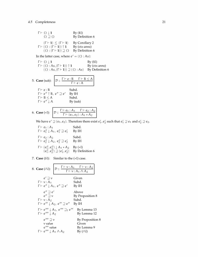
4. Case (1I): D :: Γ ` () : 1

e ′ w () is given. By the definition of w, either e ′ = () or e ′ = (() : As) for some typingannotations As. In the former case:

4.5 Completeness 21

Γ ` () ↓ 1 By (1I)() w () By Definition 6

(Γ ` 1) . (Γ ` 1) By Corollary 2Γ ` (() : (Γ ` 1)) ↑ 1 By (ctx-anno)

(() : (Γ ` 1)) w () By Definition 6

In the latter case, where e ′ = (() : As):

Γ ` () ↓ 1 By (1I)Γ ` (() : As, (Γ ` 1)) ↑ 1 By (ctx-anno)

(() : As, (Γ ` 1)) w (() : As) By Definition 6

5. Case (sub): D ::Γ ` e : B Γ ` B ≤ A

Γ ` e : A

Γ ` e : B Subd.Γ ` e ′′ ↑ B, e ′′ w e ′ By IHΓ ` B ≤ A Subd.Γ ` e ′′ ↓ A By (sub)

6. Case (∗I): D ::Γ ` e1 : A1 Γ ` e2 : A2

Γ ` (e1, e2) : A1 ∗ A2

We have e ′ w (e1, e2). Therefore there exist e ′

1, e ′

2 such that e ′

1 w e1 and e ′

2 w e2.

Γ ` e1 : A1 Subd.Γ ` e ′′

1 ↓ A1, e ′′

1 w e ′

1 By IH

Γ ` e2 : A2 Subd.Γ ` e ′′

2 ↓ A2, e ′′

2 w e ′

2 By IH

Γ ` (e ′′

1 , e ′′

2 ) ↓ A1 ∗ A2 By (∗I)(e ′′

1 , e ′′

2 ) w (e ′

1, e ′

2) By Definition 6

7. Case (δI): Similar to the (∗I) case.

8. Case (∧I): D ::Γ ` v : A1 Γ ` v : A2

Γ ` v : A1 ∧ A2

e ′ w v GivenΓ ` v : A1 Subd.Γ ` e ′′ ↓ A1, e ′′ w e ′ By IH

e ′′ w e ′ Abovee ′′ w v By Proposition 8

Γ ` v : A2 Subd.Γ ` e ′′′ ↓ A2, e ′′′ w e ′′ By IH

Γ ` e ′′′′ ↓ A1, e ′′′′ w` e ′′′ By Lemma 13Γ ` e ′′′′ ↓ A2 By Lemma 12

e ′′′′ w v By Proposition 8v value Givene ′′′′ value By Lemma 9

Γ ` e ′′′′ ↓ A1 ∧ A2 By (∧I)

22 4 CONTEXTUAL TYPING ANNOTATIONS

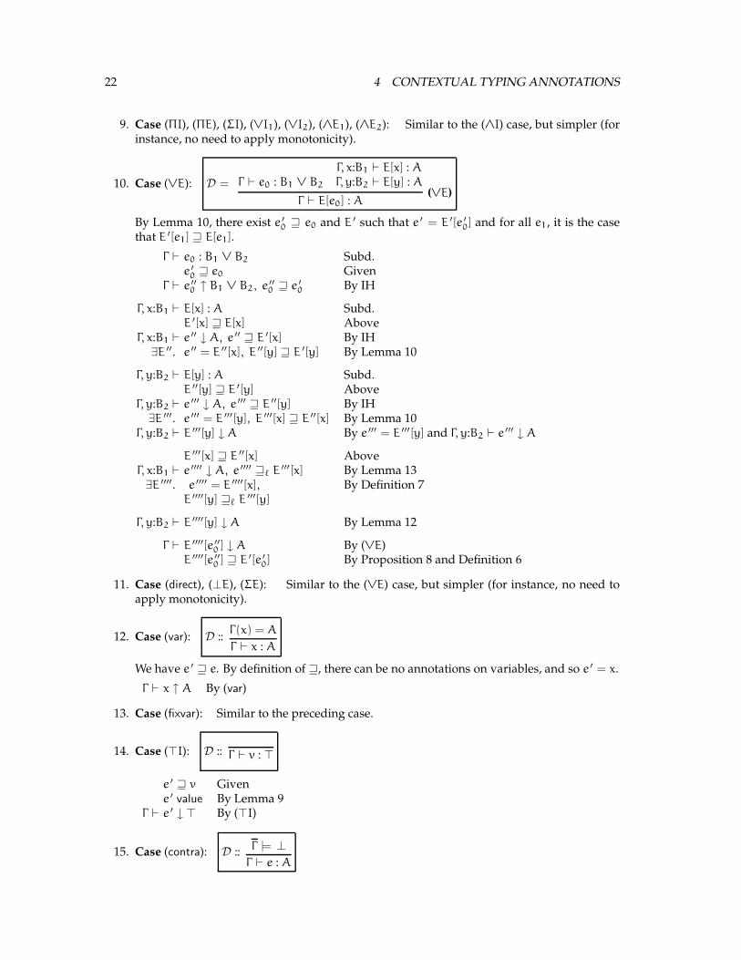
9. Case (ΠI), (ΠE), (ΣI), (∨I1), (∨I2), (∧E1), (∧E2): Similar to the (∧I) case, but simpler (forinstance, no need to apply monotonicity).

10. Case (∨E): D = Γ ` e0 : B1 ∨ B2

Γ, x:B1 ` E[x] : A

Γ, y:B2 ` E[y] : A

Γ ` E[e0] : A(∨E)

By Lemma 10, there exist e ′

0 w e0 and E ′ such that e ′ = E ′[e ′

0] and for all e1, it is the casethat E ′[e1] w E[e1].

Γ ` e0 : B1 ∨ B2 Subd.e ′

0 w e0 GivenΓ ` e ′′

0 ↑ B1 ∨ B2, e ′′

0 w e ′

0 By IH

Γ, x:B1 ` E[x] : A Subd.E ′[x] w E[x] Above

Γ, x:B1 ` e ′′ ↓ A, e ′′ w E ′[x] By IH∃E ′′. e ′′ = E ′′[x], E ′′[y] w E ′[y] By Lemma 10

Γ, y:B2 ` E[y] : A Subd.E ′′[y] w E ′[y] Above

Γ, y:B2 ` e ′′′ ↓ A, e ′′′ w E ′′[y] By IH∃E ′′′. e ′′′ = E ′′′[y], E ′′′[x] w E ′′[x] By Lemma 10

Γ, y:B2 ` E ′′′[y] ↓ A By e ′′′ = E ′′′[y] and Γ, y:B2 ` e ′′′ ↓ A

E ′′′[x] w E ′′[x] AboveΓ, x:B1 ` e ′′′′ ↓ A, e ′′′′ w` E ′′′[x] By Lemma 13∃E ′′′′. e ′′′′ = E ′′′′[x],

E ′′′′[y] w` E ′′′[y]

By Definition 7

Γ, y:B2 ` E ′′′′[y] ↓ A By Lemma 12

Γ ` E ′′′′[e ′′

0 ] ↓ A By (∨E)E ′′′′[e ′′

0 ] w E ′[e ′

0] By Proposition 8 and Definition 6

11. Case (direct), (⊥E), (ΣE): Similar to the (∨E) case, but simpler (for instance, no need toapply monotonicity).

12. Case (var): D ::Γ(x) = A

Γ ` x : A

We have e ′ w e. By definition of w, there can be no annotations on variables, and so e ′ = x.

Γ ` x ↑ A By (var)

13. Case (fixvar): Similar to the preceding case.

14. Case (>I): D :: Γ ` v : >

e ′ w v Givene ′ value By Lemma 9

Γ ` e ′ ↓ > By (>I)

15. Case (contra): D ::Γ |= ⊥

Γ ` e : A

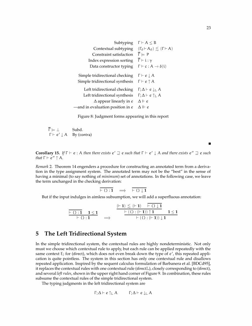
23

Subtyping Γ ` A ≤ B

Contextual subtyping (Γ0 `A0) . (Γ `A)

Constraint satisfaction Γ |= P

Index expression sorting Γ ` i : γ

Data constructor typing Γ ` c : A → δ(i)

Simple tridirectional checking Γ ` e ↓ A

Simple tridirectional synthesis Γ ` e ↑ A

Left tridirectional checking Γ ; ∆ ` e ↓L A

Left tridirectional synthesis Γ ; ∆ ` e ↑L A

∆ appear linearly in e ∆ e

—and in evaluation position in e ∆ � e

Figure 8: Judgment forms appearing in this report

Γ |= ⊥ Subd.Γ ` e ′ ↓ A By (contra)

Corollary 15. If Γ ` e : A then there exists e ′ w e such that Γ ` e ′ ↓ A and there exists e ′′ w e suchthat Γ ` e ′′ ↑ A.

Remark 2. Theorem 14 engenders a procedure for constructing an annotated term from a deriva-tion in the type assignment system. The annotated term may not be the “best” in the sense ofhaving a minimal (to say nothing of minimum) set of annotations. In the following case, we leavethe term unchanged in the checking derivation:

` () : 1 =⇒ ` () ↓ 1

But if the input indulges in aimless subsumption, we will add a superfluous annotation:

` () : 1 1 ≤ 1

` () : 1 =⇒

(` 1) . (` 1) ` () ↓ 1

` (() : (` 1)) ↑ 1 1 ≤ 1

` (() : (` 1)) ↓ 1

5 The Left Tridirectional System

In the simple tridirectional system, the contextual rules are highly nondeterministic. Not onlymust we choose which contextual rule to apply, but each rule can be applied repeatedly with thesame context E; for (direct), which does not even break down the type of e ′, this repeated appli-cation is quite pointless. The system in this section has only one contextual rule and disallowsrepeated application. Inspired by the sequent calculus formulation of Barbanera et al. [BDCd95],it replaces the contextual rules with one contextual rule (directL), closely corresponding to (direct),and several left rules, shown in the upper right hand corner of Figure 9. In combination, these rulessubsume the contextual rules of the simple tridirectional system.

The typing judgments in the left tridirectional system are

Γ ; ∆ ` e ↑L A Γ ; ∆ ` e ↓L A

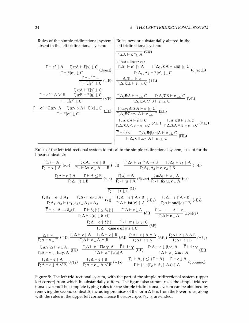
24 5 THE LEFT TRIDIRECTIONAL SYSTEM

Rules of the simple tridirectional systemabsent in the left tridirectional system:

Rules new or substantially altered in theleft tridirectional system:

Γ ; x:A ` x ↑L A(var)

Γ ` e ′ ↑ A Γ, x:A ` E[x] ↓ C

Γ ` E[e ′] ↓ C(direct)

e ′ not a linear var

Γ ; ∆1 ` e ′ ↑L A Γ ; ∆2, x:A ` E[x] ↓L C

Γ ; ∆1, ∆2 ` E[e ′] ↓L C(directL)

Γ ` e ′ ↑ ⊥

Γ ` E[e ′] ↓ C(⊥E) ∆, x:⊥ e

Γ ; ∆, x:⊥ ` e ↓L C(⊥L)

Γ ` e ′ ↑ A ∨ B

Γ, x:A ` E[x] ↓ C

Γ, y:B ` E[y] ↓ C

Γ ` E[e ′] ↓ C(∨E)

Γ ; ∆, x:A ` e ↓L C Γ ; ∆, x:B ` e ↓L C

Γ ; ∆, x:A ∨ B ` e ↓L C(∨L)

Γ ` e ′ ↑ Σa:γ. A Γ, a:γ, x:A ` E[x] ↓ C

Γ ` E[e ′] ↓ C(ΣE)

Γ, a:γ; ∆, x:A ` e ↓L C

Γ ; ∆, x:Σa:γ. A ` e ↓L C(ΣL)

Γ ; ∆, x:A ` e ↓L C

Γ ; ∆, x:A ∧ B ` e ↓L C(∧L1)

Γ ; ∆, x:B ` e ↓L C

Γ ; ∆, x:A ∧ B ` e ↓L C(∧L2)

Γ ` i : γ Γ ; ∆, x:[i/a]A ` e ↓L C

Γ ; ∆, x:Πa:γ. A ` e ↓L C(ΠL)

Rules of the left tridirectional system identical to the simple tridirectional system, except for thelinear contexts ∆:

Γ(x) = A

Γ ; · ` x ↑ A(var)

Γ, x:A; · ` e ↓ B

Γ ; · ` λx. e ↓ A → B(→I)

Γ ; ∆1 ` e1 ↑ A → B Γ ; ∆2 ` e2 ↓ A

Γ ; ∆1, ∆2 ` e1e2 ↑ B(→E)

Γ ; ∆ ` e ↑ A Γ ` A ≤ B

Γ ; ∆ ` e ↓ B(sub)

Γ(u) = A

Γ ; · ` u ↑ A(fixvar)

Γ, u:A; · ` e ↓ A

Γ ; · ` fix u. e ↓ A(fix)

Γ ; · ` () ↓ 1(1I)

Γ ; ∆1 ` e1 ↓ A1 Γ ; ∆2 ` e2 ↓ A2

Γ ; ∆1, ∆2 ` (e1, e2) ↓ A1 ∗ A2(∗I)

Γ ; ∆ ` e ↑ A ∗ B

Γ ; ∆ ` fst(e) ↑ A(∗E1)

Γ ; ∆ ` e ↑ A ∗ B

Γ ; ∆ ` snd(e) ↑ B(∗E2)

Γ ` c : A → δ2(i) Γ ` δ2(i) ≤ δ1(j) Γ ; ∆ ` e ↓ A

Γ ; ∆ ` c(e) ↓ δ1(j)(δI)

Γ |= ⊥ ∆ e

Γ ; ∆ ` e ↓ A(contra)

Γ ; ∆ ` e ↑ δ(i) Γ ; · ` ms ↓δ(i) C

Γ ; ∆ ` case e of ms ↓ C(δE)

∆ vΓ ; ∆ ` v ↓ >

(>I)Γ ; ∆ ` v ↓ A Γ ; ∆ ` v ↓ B

Γ ; ∆ ` v ↓ A ∧ B(∧I)

Γ ; ∆ ` e ↑ A ∧ B

Γ ; ∆ ` e ↑ A(∧E1)

Γ ; ∆ ` e ↑ A ∧ B

Γ ; ∆ ` e ↑ B(∧E2)

Γ, a:γ; ∆ ` v ↓ A

Γ ; ∆ ` v ↓ Πa:γ. A(ΠI)

Γ ; ∆ ` e ↑ Πa:γ. A Γ ` i : γ

Γ ; ∆ ` e ↑ [i/a] A(ΠE)

Γ ; ∆ ` e ↓ [i/a] A Γ ` i : γ

Γ ; ∆ ` e ↓ Σa:γ. A(ΣI)

Γ ; ∆ ` e ↓ A

Γ ; ∆ ` e ↓ A ∨ B(∨I1)

Γ ; ∆ ` e ↓ B

Γ ; ∆ ` e ↓ A ∨ B(∨I2)

(Γ0 ` A0) . (Γ ` A) Γ ` e ↓ A

Γ ` (e : (Γ0 ` A0), As) ↑ A(ctx-anno)

Figure 9: The left tridirectional system, with the part of the simple tridirectional system (upperleft corner) from which it substantially differs. The figure also summarizes the simple tridirec-tional system: The complete typing rules for the simple tridirectional system can be obtained byremoving the second context ∆, including premises of the form ∆ e, from the lower rules, alongwith the rules in the upper left corner. Hence the subscripts ↑L, ↓L are elided.

25

Γ ` |e| : A

Typeassignmentsystem[DP03]

Thm. 14

?

6

Thm. 3

Γ ` e ↑ A

Γ ` e ↓ A

Simpletridirectionalsystem

Thm. 24

?

6

Thm. 22

Γ ; ∆ ` e ↑L A

Γ ; ∆ ` e ↓L A

Lefttridirectionalsystem

Figure 10: Connections between our type systems

where ∆ is a linear context whose domain is a new syntactic category, the linear variables x, y andso forth. These linear variables correspond to the variables introduced in evaluation position inthe (direct) rule, and appear exactly once in the term e, in evaluation position. We consider theselinear variables to be values, like ordinary variables.

The rule (directL) is the only rule that adds to the linear context, and is the true source oflinearity: x appears exactly once in evaluation position in E[x]. It requires that the subterm e ′

being brought out cannot itself be a linear variable, so one cannot bring out a term more thanonce, unlike with (direct).

To maintain linearity, the linear context is split among subterms. For example, in (∗I) (Figure9), the context ∆ = ∆1, ∆2 is split between e1 and e2. To maintain the property that linear variablesappear in evaluation position, in rules such as (→I) that type terms that cannot contain a variable,the linear context is empty.

After some preliminary definitions and lemmas, we prove that this new left tridirectional systemis sound and complete with respect to the simple tridirectional system from Section 3. (See alsoFigure 10).

Definition 16. Let FLV(e) denote the set of linear variables appearing free in e. Furthermore, let ∆ e ifand only if (1) for every x ∈ dom(∆), x appears exactly once in e, and (2) FLV(e) ⊆ dom(∆). (Similarlydefine FLV(ms) and ∆ ms.)

Proposition 17 (Linearity). If Γ ; ∆ ` e ↑L C or Γ ; ∆ ` e ↓L C then ∆ e. Similarly, if Γ ; ∆ ` ms ↓δ(i)

C then ∆ ms.

Proof. By induction on the derivation. For (contra), (>I), (⊥L), use the appropriate premise. Forall cases in which the term and linear context of each premise are the same as the term and linearcontext of the conclusion, simply apply the IH. Cases which decompose the term (such as (∗E1))require an additional step, such as from ∆ e ′ to ∆ fst(e ′); the cases for matches all haveempty linear contexts.

Definition 18. Let ∆ � e if and only if (1) for every x ∈ dom(∆), there exists an E such that e = E[x]

and x /∈ FLV(E), and (2) FLV(e) ⊆ dom(∆). (It is clear that ∆ � e implies ∆ e.)

Remark 3. Note that the assertion

“If Γ ; ∆ ` e ↑L C or Γ ; ∆ ` e ↓L C then ∆ � e”

does not hold. Suppose Γ ; x ` x(e2e3) ↑L A → B and Γ ; y ` y ↓L A. It is the case that x � x(e2e3)

and y � y. We can apply (→E) to get Γ ; x, y ` (x(e2e3)) y, but y is not in evaluation position in(x(e2e3)) y so we do not have x, y � (x(e2e3)) y. However, the following lemma does hold.

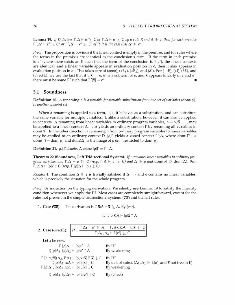
26 5 THE LEFT TRIDIRECTIONAL SYSTEM

Lemma 19. If D derives Γ ; ∆ ` e ↑L C or Γ ; ∆ ` e ↓L C by a rule R and ∆ � e, then for each premiseΓ ′; ∆ ′ ` e ′ ↑L C ′ or Γ ′; ∆ ′ ` e ′ ↓L C ′ of R, it is the case that ∆ ′ � e ′.

Proof. The proposition is obvious if the linear context is empty in the premise, and for rules wherethe terms in the premises are identical to the conclusion’s term. If the term in each premiseis e ′ where there exists an E such that the term of the conclusion is E[e ′], the linear contextsare identical, and a linear variable appears in evaluation position in e, then it also appears inevaluation position in e ′. This takes care of (anno), (∗E1), (∗E2), and (δI). For (→E), (∗I), (δE), and(directL), we use the fact that if E[x] = e, e ′ is a subterm of e, and x appears linearly in e and e ′,there must be some E ′ such that E ′[x] = e ′.

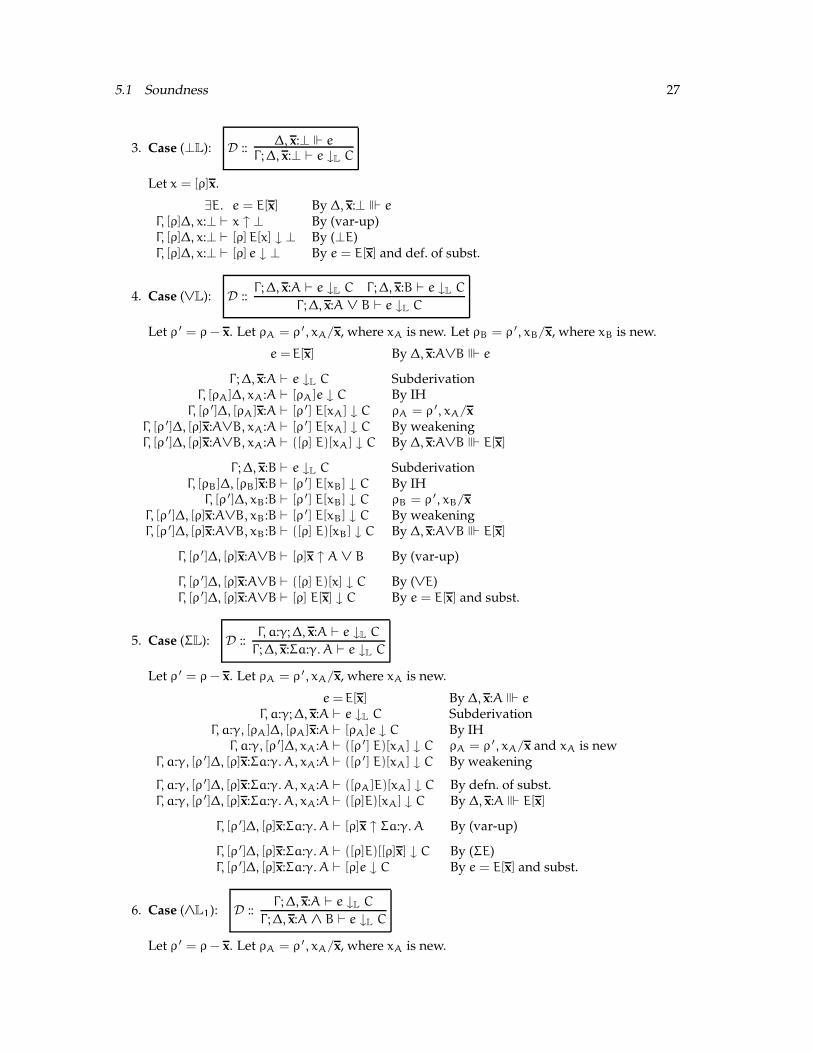
5.1 Soundness

Definition 20. A renaming ρ is a variable-for-variable substitution from one set of variables (dom(ρ))to another, disjoint set.

When a renaming is applied to a term, [ρ]e, it behaves as a substitution, and can substitutethe same variable for multiple variables. Unlike a substitution, however, it can also be appliedto contexts. A renaming from linear variables to ordinary program variables, ρ = x/x, . . . , maybe applied to a linear context ∆: [ρ]∆ yields an ordinary context Γ by renaming all variables indom(∆). In the other direction, a renaming ρ from ordinary program variables to linear variablesmay be applied to an ordinary context Γ : [ρ]Γ yields a zoned context Γ ′; ∆, where dom(Γ ′) =

dom(Γ) − dom(ρ) and dom(∆) is the image of ρ on Γ restricted to dom(ρ).

Definition 21. ρ⇓Γ denotes ∆ where [ρ]Γ = Γ ′; ∆.

Theorem 22 (Soundness, Left Tridirectional System). If ρ renames linear variables to ordinary pro-gram variables and Γ ; ∆ ` e ↑L C (resp. Γ ; ∆ ` e ↓L C) and ∆ � e and dom(ρ) ⊇ dom(∆), thenΓ, [ρ]∆ ` [ρ]e ↑ C (resp. Γ, [ρ]∆ ` [ρ]e ↓ C).

Remark 4. The condition ∆ � e is trivially satisfied if ∆ = · and e contains no linear variables,which is precisely the situation for the whole program.

Proof. By induction on the typing derivation. We silently use Lemma 19 to satisfy the linearitycondition whenever we apply the IH. Most cases are completely straightforward, except for therules not present in the simple tridirectional system: (var) and the left rules.

1. Case (var): The derivation is Γ ; x:A ` x ↑L A. By (var),

[ρ]Γ, [ρ]x:A ` [ρ]x ↑ A

2. Case (directL): D ::Γ ; ∆1 ` e ′ ↑L A Γ ; ∆2, x:A ` E[x] ↓L C

Γ ; ∆1, ∆2 ` E[e ′] ↓L C

Let x be new.

Γ, [ρ]∆1 ` [ρ]e ′ ↑ A By IHΓ, [ρ]∆1, [ρ]∆2 ` [ρ]e ′ ↑ A By weakening

Γ, [ρ, x/x](∆2, x:A) ` [ρ, x/x] E[x] ↓ C By IHΓ, [ρ]∆2, x:A ` [ρ] E[x] ↓ C By def. of subst. (∆1, ∆2 � E[e ′] and x not free in E)

Γ, [ρ]∆1, [ρ]∆2, x:A ` [ρ] E[x] ↓ C By weakening

Γ, [ρ]∆1, [ρ]∆2 ` [ρ] E[e ′] ↓ C By (direct)

5.1 Soundness 27

3. Case (⊥L): D ::∆, x:⊥ e

Γ ; ∆, x:⊥ ` e ↓L C

Let x = [ρ]x.

∃E. e = E[x] By ∆, x:⊥ � e

Γ, [ρ]∆, x:⊥ ` x ↑ ⊥ By (var-up)Γ, [ρ]∆, x:⊥ ` [ρ] E[x] ↓ ⊥ By (⊥E)Γ, [ρ]∆, x:⊥ ` [ρ] e ↓ ⊥ By e = E[x] and def. of subst.

4. Case (∨L): D ::Γ ; ∆, x:A ` e ↓L C Γ ; ∆, x:B ` e ↓L C

Γ ; ∆, x:A ∨ B ` e ↓L C

Let ρ ′ = ρ − x. Let ρA = ρ ′, xA/x, where xA is new. Let ρB = ρ ′, xB/x, where xB is new.

e =E[x] By ∆, x:A∨B � e

Γ ; ∆, x:A ` e ↓L C SubderivationΓ, [ρA]∆, xA:A ` [ρA]e ↓ C By IH

Γ, [ρ ′]∆, [ρA]x:A ` [ρ ′] E[xA] ↓ C ρA = ρ ′, xA/xΓ, [ρ ′]∆, [ρ]x:A∨B, xA:A ` [ρ ′] E[xA] ↓ C By weakeningΓ, [ρ ′]∆, [ρ]x:A∨B, xA:A ` ([ρ] E)[xA] ↓ C By ∆, x:A∨B � E[x]

Γ ; ∆, x:B ` e ↓L C SubderivationΓ, [ρB]∆, [ρB]x:B ` [ρ ′] E[xB] ↓ C By IH

Γ, [ρ ′]∆, xB:B ` [ρ ′] E[xB] ↓ C ρB = ρ ′, xB/xΓ, [ρ ′]∆, [ρ]x:A∨B, xB:B ` [ρ ′] E[xB] ↓ C By weakeningΓ, [ρ ′]∆, [ρ]x:A∨B, xB:B ` ([ρ] E)[xB] ↓ C By ∆, x:A∨B � E[x]

Γ, [ρ ′]∆, [ρ]x:A∨B ` [ρ]x ↑ A ∨ B By (var-up)

Γ, [ρ ′]∆, [ρ]x:A∨B ` ([ρ] E)[x] ↓ C By (∨E)Γ, [ρ ′]∆, [ρ]x:A∨B ` [ρ] E[x] ↓ C By e = E[x] and subst.

5. Case (ΣL): D ::Γ, a:γ; ∆, x:A ` e ↓L C

Γ ; ∆, x:Σa:γ. A ` e ↓L C

Let ρ ′ = ρ − x. Let ρA = ρ ′, xA/x, where xA is new.

e = E[x] By ∆, x:A � e

Γ, a:γ; ∆, x:A ` e ↓L C SubderivationΓ, a:γ, [ρA]∆, [ρA]x:A ` [ρA]e ↓ C By IH

Γ, a:γ, [ρ ′]∆, xA:A ` ([ρ ′] E)[xA] ↓ C ρA = ρ ′, xA/x and xA is newΓ, a:γ, [ρ ′]∆, [ρ]x:Σa:γ. A, xA:A ` ([ρ ′] E)[xA] ↓ C By weakening

Γ, a:γ, [ρ ′]∆, [ρ]x:Σa:γ. A, xA:A ` ([ρA]E)[xA] ↓ C By defn. of subst.Γ, a:γ, [ρ ′]∆, [ρ]x:Σa:γ. A, xA:A ` ([ρ]E)[xA] ↓ C By ∆, x:A � E[x]

Γ, [ρ ′]∆, [ρ]x:Σa:γ. A ` [ρ]x ↑ Σa:γ. A By (var-up)

Γ, [ρ ′]∆, [ρ]x:Σa:γ. A ` ([ρ]E)[[ρ]x] ↓ C By (ΣE)Γ, [ρ ′]∆, [ρ]x:Σa:γ. A ` [ρ]e ↓ C By e = E[x] and subst.

6. Case (∧L1): D ::Γ ; ∆, x:A ` e ↓L C

Γ ; ∆, x:A ∧ B ` e ↓L C

Let ρ ′ = ρ − x. Let ρA = ρ ′, xA/x, where xA is new.

28 5 THE LEFT TRIDIRECTIONAL SYSTEM

e = E[x] By ∆, x:A ∧ B � e

Γ ; ∆, x:A ` e ↓L C SubderivationΓ, [ρA]∆, [ρA]x:A ` [ρA]e ↓ C By IH

Γ, [ρ ′]∆, xA:A ` ([ρ ′] E)[xA] ↓ C ρA = ρ ′, xA/x and xA is newΓ, [ρ ′]∆, [ρ]x:A∧B, xA:A ` ([ρ ′] E)[xA] ↓ C By weakeningΓ, [ρ ′]∆, [ρ]x:A∨B, xA:A ` ([ρ] E)[xA] ↓ C By ∆, x:A∧B � E[x]

Γ, [ρ ′]∆, [ρ]x:A∧B ` [ρ]x ↑ A ∧ B By (var-up)Γ, [ρ ′]∆, [ρ]x:A∧B ` [ρ]x ↑ A By (∧E1)

Γ, [ρ ′]∆, [ρ]x:A∧B ` ([ρ] E)[xA] ↓ C By (direct)Γ, [ρ ′]∆, [ρ]x:A∧B ` [ρ]e ↓ C By e = E[x] and subst.

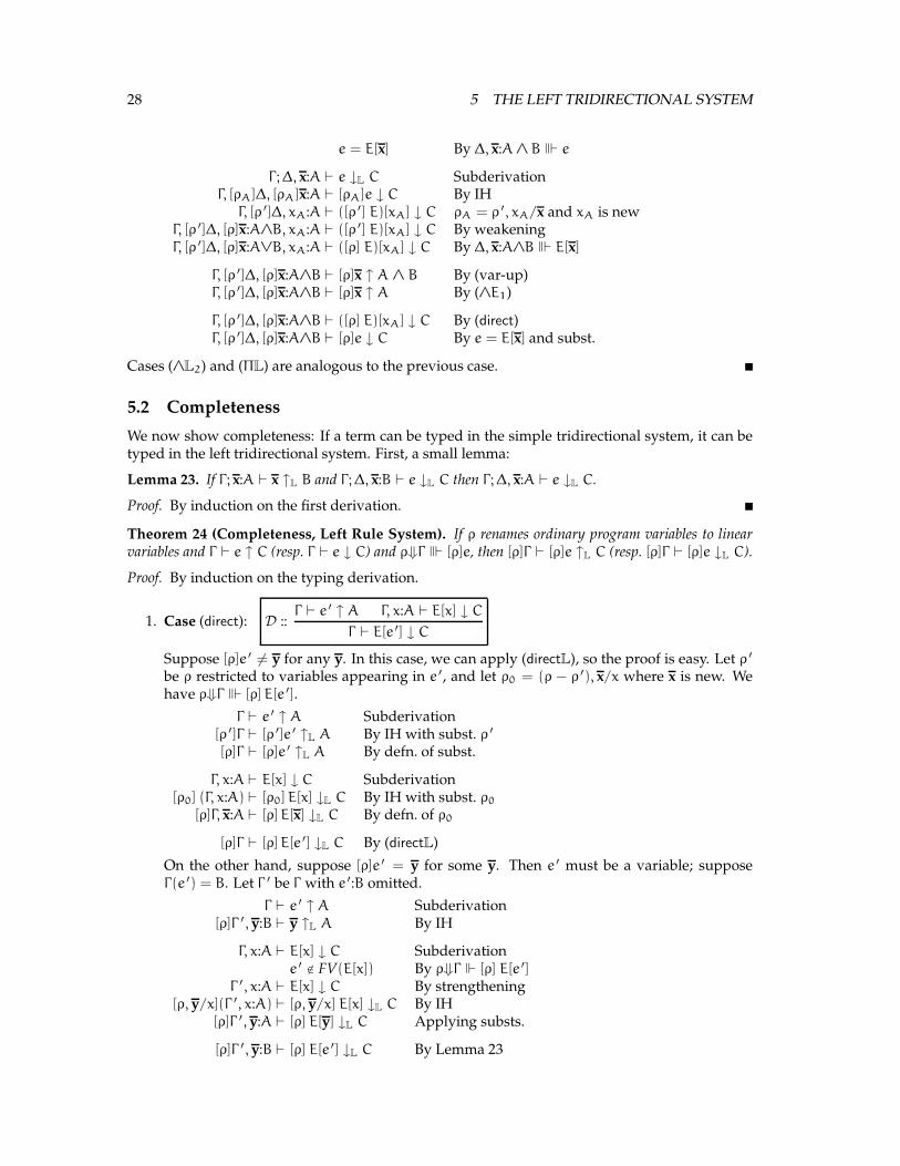
Cases (∧L2) and (ΠL) are analogous to the previous case.

5.2 Completeness

We now show completeness: If a term can be typed in the simple tridirectional system, it can betyped in the left tridirectional system. First, a small lemma:

Lemma 23. If Γ ; x:A ` x ↑L B and Γ ; ∆, x:B ` e ↓L C then Γ ; ∆, x:A ` e ↓L C.

Proof. By induction on the first derivation.

Theorem 24 (Completeness, Left Rule System). If ρ renames ordinary program variables to linearvariables and Γ ` e ↑ C (resp. Γ ` e ↓ C) and ρ⇓Γ � [ρ]e, then [ρ]Γ ` [ρ]e ↑L C (resp. [ρ]Γ ` [ρ]e ↓L C).

Proof. By induction on the typing derivation.

1. Case (direct): D ::Γ ` e ′ ↑ A Γ, x:A ` E[x] ↓ C

Γ ` E[e ′] ↓ C

Suppose [ρ]e ′ 6= y for any y. In this case, we can apply (directL), so the proof is easy. Let ρ ′

be ρ restricted to variables appearing in e ′, and let ρ0 = (ρ − ρ ′), x/x where x is new. Wehave ρ⇓Γ � [ρ] E[e ′].

Γ ` e ′ ↑ A Subderivation[ρ ′]Γ ` [ρ ′]e ′ ↑L A By IH with subst. ρ ′

[ρ]Γ ` [ρ]e ′ ↑L A By defn. of subst.

Γ, x:A ` E[x] ↓ C Subderivation[ρ0] (Γ, x:A) ` [ρ0] E[x] ↓L C By IH with subst. ρ0

[ρ]Γ, x:A ` [ρ] E[x] ↓L C By defn. of ρ0

[ρ]Γ ` [ρ] E[e ′] ↓L C By (directL)

On the other hand, suppose [ρ]e ′ = y for some y. Then e ′ must be a variable; supposeΓ(e ′) = B. Let Γ ′ be Γ with e ′:B omitted.

Γ ` e ′ ↑ A Subderivation[ρ]Γ ′, y:B ` y ↑L A By IH

Γ, x:A ` E[x] ↓ C Subderivatione ′ /∈ FV(E[x]) By ρ⇓Γ [ρ] E[e ′]

Γ ′, x:A ` E[x] ↓ C By strengthening[ρ, y/x](Γ ′, x:A) ` [ρ, y/x] E[x] ↓L C By IH

[ρ]Γ ′, y:A ` [ρ] E[y] ↓L C Applying substs.

[ρ]Γ ′, y:B ` [ρ] E[e ′] ↓L C By Lemma 23

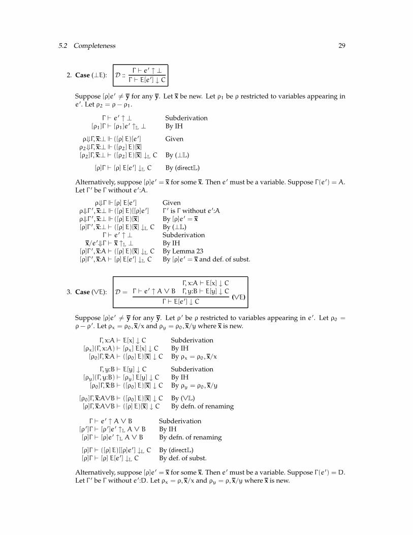
5.2 Completeness 29

2. Case (⊥E): D ::Γ ` e ′ ↑ ⊥

Γ ` E[e ′] ↓ C

Suppose [ρ]e ′ 6= y for any y. Let x be new. Let ρ1 be ρ restricted to variables appearing ine ′. Let ρ2 = ρ − ρ1.

Γ ` e ′ ↑ ⊥ Subderivation[ρ1]Γ ` [ρ1]e ′ ↑L ⊥ By IH

ρ⇓Γ, x:⊥ ([ρ] E)[e ′] Givenρ2⇓Γ, x:⊥ ([ρ2] E)[x]

[ρ2]Γ, x:⊥ ` ([ρ2] E)[x] ↓L C By (⊥L)

[ρ]Γ ` [ρ] E[e ′] ↓L C By (directL)

Alternatively, suppose [ρ]e ′ = x for some x. Then e ′ must be a variable. Suppose Γ(e ′) = A.Let Γ ′ be Γ without e ′:A.

ρ⇓Γ [ρ] E[e ′] Givenρ⇓Γ ′, x:⊥ ([ρ] E)[[ρ]e ′] Γ ′ is Γ without e ′:A

ρ⇓Γ ′, x:⊥ ([ρ] E)[x] By [ρ]e ′ = x[ρ]Γ ′, x:⊥ ` ([ρ] E)[x] ↓L C By (⊥L)

Γ ` e ′ ↑ ⊥ Subderivationx/e ′⇓Γ ` x ↑L ⊥ By IH

[ρ]Γ ′, x:A ` ([ρ] E)[x] ↓L C By Lemma 23[ρ]Γ ′, x:A ` [ρ] E[e ′] ↓L C By [ρ]e ′ = x and def. of subst.

3. Case (∨E): D = Γ ` e ′ ↑ A ∨ B

Γ, x:A ` E[x] ↓ C

Γ, y:B ` E[y] ↓ C

Γ ` E[e ′] ↓ C(∨E)

Suppose [ρ]e ′ 6= y for any y. Let ρ ′ be ρ restricted to variables appearing in e ′. Let ρ0 =

ρ − ρ ′. Let ρx = ρ0, x/x and ρy = ρ0, x/y where x is new.

Γ, x:A ` E[x] ↓ C Subderivation[ρx](Γ, x:A) ` [ρx] E[x] ↓ C By IH

[ρ0]Γ, x:A ` ([ρ0] E)[x] ↓ C By ρx = ρ0, x/x

Γ, y:B ` E[y] ↓ C Subderivation[ρy](Γ, y:B) ` [ρy] E[y] ↓ C By IH

[ρ0]Γ, x:B ` ([ρ0] E)[x] ↓ C By ρy = ρ0, x/y

[ρ0]Γ, x:A∨B ` ([ρ0] E)[x] ↓ C By (∨L)[ρ]Γ, x:A∨B ` ([ρ] E)[x] ↓ C By defn. of renaming

Γ ` e ′ ↑ A ∨ B Subderivation[ρ ′]Γ ` [ρ ′]e ′ ↑L A ∨ B By IH[ρ]Γ ` [ρ]e ′ ↑L A ∨ B By defn. of renaming

[ρ]Γ ` ([ρ] E)[[ρ]e ′] ↓L C By (directL)[ρ]Γ ` [ρ] E[e ′] ↓L C By def. of subst.

Alternatively, suppose [ρ]e ′ = x for some x. Then e ′ must be a variable. Suppose Γ(e ′) = D.Let Γ ′ be Γ without e ′:D. Let ρx = ρ, x/x and ρy = ρ, x/y where x is new.

30 5 THE LEFT TRIDIRECTIONAL SYSTEM

Γ, x:A ` E[x] ↓ C Subderivation[ρx]Γ ′, x:A ` [ρx] E[x] ↓ C By IH[ρ]Γ ′, x:A ` [ρ] E[x] ↓ C By defn. of renaming

Γ, y:B ` E[y] ↓ C Subderivation[ρy]Γ ′, x:B ` [ρy] E[y] ↓ C By IH[ρ]Γ ′, x:B ` [ρ] E[x] ↓ C By defn. of renaming

[ρ]Γ ′, x:A∨B ` ([ρ] E)[x] ↓L C By (∨L)

Γ ` e ′ ↑ A ∨ B Subderivationx/e ′⇓Γ ` x ↑L A ∨ B By IH

[ρ]Γ ′, x:A ` ([ρ] E)[x] ↓L C By Lemma 23[ρ]Γ ′, x:A ` [ρ] E[e ′] ↓L C By defn. of renaming

4. Case (ΣE): Similar to the previous case.

5. Case (→E): D ::Γ ` e1 ↑ A → C Γ ` e2 ↓ A

Γ ` e1e2 ↑ C

Let ρ1 and ρ2 be ρ restricted to variables appearing in e1 and e2 respectively.

ρ⇓Γ � e1e2 Givenρ1⇓Γ � e1 By defn. of evaluation contextsρ2⇓Γ � e2 By defn. of evaluation contexts

Γ ` e1 ↑ A → C Subderivation[ρ1]Γ ` [ρ1]e1 ↑L A → C By IH

Γ ` e2 ↓ A Subderivation[ρ2]Γ ` [ρ2]e2 ↓L A By IH

[ρ]Γ ` [ρ] e1e2 ↑L C By (→E)

5.3 Decidability of Typing

Theorem 25. Γ ; ∆ ` e ↓L A is decidable.

Proof. We impose an order < on two judgments J1 = Γ1; ∆1 ` e1 ↓↑ A1 and J2 = Γ2; ∆2 `e2 ↓↑ A2. When ordering terms, we consider linear variables to be smaller than any other terms;for example, (x, e2) is smaller than (y, e2)). When ordering types (that is, type expressions), weconsider all index expressions to be of equal size.

The order is defined as follows.

1. If e1 is smaller than e2 then J1 < J2. If e1 is the same size as e2:

2. If the directions of the judgments differ, the synthesis judgment is smaller than the checkingjudgment. If the directions are the same:

3. If both judgments are checking judgments and A1 is smaller than A2 then J1 < J2. If bothjudgments are synthesis judgments, Γ1 = Γ2, ∆1 = ∆2, A1 is at least as small as some typein Γ1; ∆1 and A1 is larger than A2, then J1 < J2. Otherwise:

4. If the number of times any of the type constructors ∨, Σ, ⊥, ∧, Π, > appear in ∆1 is less thanthe number of times they appear in ∆2 then J1 < J2.

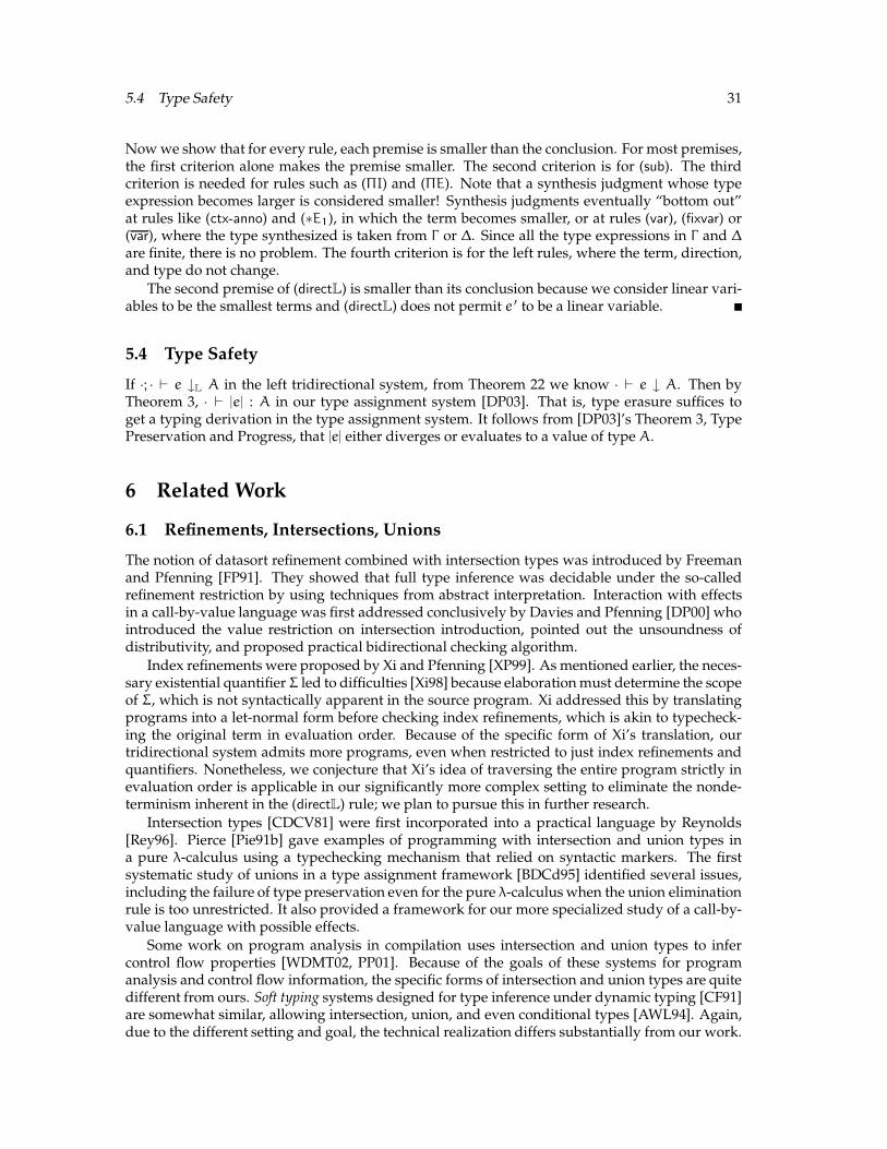
5.4 Type Safety 31

Now we show that for every rule, each premise is smaller than the conclusion. For most premises,the first criterion alone makes the premise smaller. The second criterion is for (sub). The thirdcriterion is needed for rules such as (ΠI) and (ΠE). Note that a synthesis judgment whose typeexpression becomes larger is considered smaller! Synthesis judgments eventually “bottom out”at rules like (ctx-anno) and (∗E1), in which the term becomes smaller, or at rules (var), (fixvar) or(var), where the type synthesized is taken from Γ or ∆. Since all the type expressions in Γ and ∆

are finite, there is no problem. The fourth criterion is for the left rules, where the term, direction,and type do not change.

The second premise of (directL) is smaller than its conclusion because we consider linear vari-ables to be the smallest terms and (directL) does not permit e ′ to be a linear variable.

5.4 Type Safety

If ·; · ` e ↓L A in the left tridirectional system, from Theorem 22 we know · ` e ↓ A. Then byTheorem 3, · ` |e| : A in our type assignment system [DP03]. That is, type erasure suffices toget a typing derivation in the type assignment system. It follows from [DP03]’s Theorem 3, TypePreservation and Progress, that |e| either diverges or evaluates to a value of type A.

6 Related Work

6.1 Refinements, Intersections, Unions

The notion of datasort refinement combined with intersection types was introduced by Freemanand Pfenning [FP91]. They showed that full type inference was decidable under the so-calledrefinement restriction by using techniques from abstract interpretation. Interaction with effectsin a call-by-value language was first addressed conclusively by Davies and Pfenning [DP00] whointroduced the value restriction on intersection introduction, pointed out the unsoundness ofdistributivity, and proposed practical bidirectional checking algorithm.

Index refinements were proposed by Xi and Pfenning [XP99]. As mentioned earlier, the neces-sary existential quantifier Σ led to difficulties [Xi98] because elaboration must determine the scopeof Σ, which is not syntactically apparent in the source program. Xi addressed this by translatingprograms into a let-normal form before checking index refinements, which is akin to typecheck-ing the original term in evaluation order. Because of the specific form of Xi’s translation, ourtridirectional system admits more programs, even when restricted to just index refinements andquantifiers. Nonetheless, we conjecture that Xi’s idea of traversing the entire program strictly inevaluation order is applicable in our significantly more complex setting to eliminate the nonde-terminism inherent in the (directL) rule; we plan to pursue this in further research.

Intersection types [CDCV81] were first incorporated into a practical language by Reynolds[Rey96]. Pierce [Pie91b] gave examples of programming with intersection and union types ina pure λ-calculus using a typechecking mechanism that relied on syntactic markers. The firstsystematic study of unions in a type assignment framework [BDCd95] identified several issues,including the failure of type preservation even for the pure λ-calculus when the union eliminationrule is too unrestricted. It also provided a framework for our more specialized study of a call-by-value language with possible effects.

Some work on program analysis in compilation uses intersection and union types to infercontrol flow properties [WDMT02, PP01]. Because of the goals of these systems for programanalysis and control flow information, the specific forms of intersection and union types are quitedifferent from ours. Soft typing systems designed for type inference under dynamic typing [CF91]are somewhat similar, allowing intersection, union, and even conditional types [AWL94]. Again,due to the different setting and goal, the technical realization differs substantially from our work.

32 7 CONCLUSION

6.2 Partial Inference Systems

Our system shares several properties with Pierce and Turner’s local type inference [PT98]. Theirlanguage has subtyping and impredicative polymorphism, making full type inference undecid-able. Their partial inference strategy is formulated as a bidirectional system with synthesis andchecking judgments, in a style not too far removed from ours. However, in order to handleparametric polymorphism without using nonlocal methods such as unification, they infer typearguments to polymorphic functions, which seems to substantially complicate matters. Hosoyaand Pierce [HP99] further discuss this style, particularly its effectiveness in achieving a reasonablenumber of annotations.

Our system does not yet have parametric polymorphism. Prior research, either with (in [Xi98])or without (in [DP00]) a syntactic distinction between ordinary and property types, is not conclu-sive. However, the work on local type inference suggests that, at least, prefix polymorphism inthe style of ML should be amenable to a consistent treatment with bidirectional rules.

6.3 Principal Typings

A principal type of e is a type that represents all types of e—in some particular context Γ . Aprincipal typing [Jim95] of e is a pair (Γ, A) of a context and a type, such that (Γ, A) represents allpairs (Γ ′, A ′) such that Γ ′ ` e : A ′. These definitions depend on some idea of representation,which varies from type system to type system, making comparisons between systems difficult.Wells [Wel02] improved the situation by introducing a general notion of representation. Sincefull type inference seems in any case unattainable, we have not investigated whether principaltypings might exist for our language. However, the idea of assigning a typing (rather than justa type) to a term appears in our system in the form of contextual typing annotations, enablingus to solve some otherwise very unpleasant problems regarding the scope of quantified indexvariables.

7 Conclusion

In [DP03], we developed a type assignment system with a rich set of property type constructors.That system is sound in a standard call-by-value semantics, but is inherently undecidable. In thispaper, by taking a tridirectional version of the type assignment system, we have obtained a richyet decidable type system. Every program well-typed under the type assignment system has anannotation with contextual typings that checks under the tridirectional rules. Contextual typingannotations should be useful in other settings, such as systems of parametric polymorphism inwhich subtyping is decidable.

In order to show decidability, and as a first important step towards a practical implementation,we also presented a less nondeterministic left tridirectional system and proved it to be decidable andsound and complete with respect to the tridirectional system.

We are in the process of formulating a let-normal version of the left tridirectional system. Sucha system would drastically reduce the nondeterminism in (directL) by forcing the typechecker totraverse subterms in evaluation order, while being sound and complete with respect to the lefttridirectional system.

Once this is done, we plan to develop a prototype implementation of the let-normal systemthat should help us answer questions regarding the practicality of our design on realistic pro-grams. The main questions will be (1) if the required annotations are reasonable in size, (2) if typechecking is efficient enough for interesting program properties, and (3) if the typing discipline isaccurate enough to track properties in complex programs. The preliminary experience with typerefinements, including both datasort refinements [Dav97a] and index refinements [XP99], givessome reasons for optimism, but more research and experimentation is needed.

REFERENCES 33

Acknowledgments

This work supported in part by the National Science Foundation under grant CCR-0204248; thefirst author was also supported in part by an NSF Graduate Research Fellowship. We thankJonathan Moody, Sungwoo Park, and the anonymous reviewers for their useful comments on thePOPL version of this report [DP04]. We would also like to thank Rowan Davies for many fruitfuldiscussions regarding the subject of this report.

References

[AWL94] Alexander Aiken, Edward L. Wimmers, and T. K. Lakshman. Soft typing with con-ditional types. In ACM Symp. Principles of Programming Languages, pages 163–173,1994.

[BDCd95] Franco Barbanera, Mariangiola Dezani-Ciancaglini, and Ugo de’Liguoro. Intersec-tion and union types: syntax and semantics. Inf. and Comp., 119:202–230, 1995.

[CDCV81] M. Coppo, M. Dezani-Ciancaglini, and B. Venneri. Functional characters of solvableterms. Zeitschrift f. math. Logik und Grundlagen d. Math., 27:45–58, 1981.

[CF91] Robert Cartwright and Mike Fagan. Soft typing. In SIGPLAN Conf. ProgrammingLanguage Design and Impl. (PLDI), volume 26, pages 278–292, 1991.

[Dav97a] Rowan Davies. A practical refinement-type checker for Standard ML. In AlgebraicMethodology and Software Tech. (AMAST’97), pages 565–566. Springer LNCS 1349,1997.

[Dav97b] Rowan Davies. Practical refinement-type checking. PhD thesis proposal, CarnegieMellon University, 1997.

[DP00] Rowan Davies and Frank Pfenning. Intersection types and computational effects. InInt’l Conf. Functional Programming (ICFP ’00), pages 198–208, 2000.

[DP03] Joshua Dunfield and Frank Pfenning. Type assignment for intersections and unionsin call-by-value languages. In Found. Software Science and Computation Structures(FOSSACS ’03), pages 250–266, Warsaw, Poland, April 2003. Springer LNCS 2620.

[DP04] Joshua Dunfield and Frank Pfenning. Tridirectional typechecking. In Xavier Leroy,editor, ACM Symp. Principles of Programming Languages (POPL ’04), pages 281–292,Venice, Italy, January 2004.

[Dun02] Joshua Dunfield. Combining two forms of type refinements. Technical Report CMU-CS-02-182, Carnegie Mellon University, September 2002.

[FP91] Tim Freeman and Frank Pfenning. Refinement types for ML. In SIGPLAN Conf. Pro-gramming Language Design and Impl. (PLDI), volume 26, pages 268–277. ACM Press,1991.

[Fre94] Tim Freeman. Refinement types for ML. PhD thesis, Carnegie Mellon University, 1994.CMU-CS-94-110.

[HP99] Haruo Hosoya and Benjamin C. Pierce. How good is local type inference? TechnicalReport MS-CIS-99-17, University of Pennsylvania, June 1999.

[Jim95] Trevor Jim. What are principal typings and what are they good for? Technical mem-orandum MIT/LCS/TM-532, MIT, November 1995.

34 REFERENCES

[MWH02] Yitzhak Mandelbaum, David Walker, and Robert Harper. An effective theory of typerefinements. Technical Report TR-656-02, Princeton, December 2002.

[Pie91a] Benjamin C. Pierce. Programming with intersection types and bounded polymorphism.PhD thesis, Carnegie Mellon University, 1991. Technical Report CMU-CS-91-205.

[Pie91b] Benjamin C. Pierce. Programming with intersection types, union types, and poly-morphism. Technical Report CMU-CS-91-106, Carnegie Mellon University, 1991.

[PP01] Jens Palsberg and Christina Pavlopoulou. From polyvariant flow information to in-tersection and union types. J. Func. Prog., 11(3):263–317, 2001.

[PT98] Benjamin C. Pierce and David N. Turner. Local type inference. In ACM Symp. Princi-ples of Programming Languages, pages 252–265, 1998. Full version in ACM Trans. Prog.Lang. Sys., 22(1):1–44, 2000.

[Rey96] John C. Reynolds. Design of the programming language Forsythe. Technical ReportCMU-CS-96-146, Carnegie Mellon University, 1996.

[SWM00] Fred Smith, David Walker, and Greg Morrisett. Alias types. In European Symp. onProgramming (ESOP’00), pages 366–381, Berlin, Germany, March 2000.

[TJ94] Jean-Pierre Talpin and Pierre Jouvelot. The type and effect discipline. Inf. and Comp.,111(2):245–296, 1994.

[TT97] Mads Tofte and Jean-Pierre Talpin. Region-based memory management. Inf. andComp., 132(2):109–176, 1997.

[WDMT02] J.B. Wells, Allyn Dimock, Robert Muller, and Franklyn Turbak. A calculus with poly-morphic and polyvariant flow types. J. Func. Prog., 12(3):183–317, May 2002.

[Wel02] J.B. Wells. The essence of principal typings. In Int’l Coll. Automata, Languages, andProgramming, volume 2380 of LNCS, pages 913–925. Springer, 2002.

[WH02] J. B. Wells and Christian Haack. Branching types. In European Symp. on Programming(ESOP’02), pages 115–132, 2002.

[Xi98] Hongwei Xi. Dependent types in practical programming. PhD thesis, Carnegie MellonUniversity, 1998.

[Xi00] Hongwei Xi. Dependently typed data structures. Revision superseding WAAAPL’99, February 2000.

[XP99] Hongwei Xi and Frank Pfenning. Dependent types in practical programming. InACM Symp. Principles of Programming Languages, pages 214–227, 1999.