CDE September 2012

TRENDS IN TOTAL FACTOR PRODUCTIVITY IN

INDIAN AGRICULTURE: STATE-LEVEL EVIDENCE USING NON-PARAMETRIC SEQUENTIAL

MALMQUIST INDEX

SHILPA CHAUDHARY

Email: shilpa@econdse.org Delhi School of Economics

University of Delhi

Working Paper No. 215

Centre for Development Economics

Department of Economics, Delhi School of Economics

Trends in Total Factor Productivity in Indian Agriculture: State-level Evidence using non-parametric Sequential Malmquist

Index

Shilpa Chaudhary

Abstract

Recognizing the critical role of agricultural sector in the overall growth as well as development performance, this study estimates total factor productivity (TFP) in Indian agriculture at state-level. Using Index of Agricultural Production as the measure of output, changes in TFP are estimated using non-parametric Sequential Malmquist TFP index. The TFP change is decomposed into efficiency change and technical change. It is found that productivity improvements are marked in very few states, and so is technical change. The improvements in efficiency are observed to be low for most of the states and efficiency decline is observed in several states implying huge gains in production possible even with existing technology. In order to achieve higher productivity, it is essential to increase efficiency levels as well as achieve a more even spread of new technology.

Section I: Introduction

A rise in production can be attributed to a growth in inputs or growth in total factor productivity. The level of Total Factor Productivity (TFP) can be measured by dividing total output by total inputs. When all inputs in the production process are accounted for, TFP growth can be thought of as the amount of growth in real output that is not explained by growth in inputs. Productivity growth encompasses changes in efficiency as well as changes in the best practice. A firm is fully technically efficient if it is operating on the production frontier (i.e. it is achieving best practice), the production frontier being defined for a reference time period with reference to a particular set of firms. A rise in efficiency implies either more output is produced with the same amount of inputs or that less inputs are required to produce the same level of output. Equally, the outward shift of a production frontier implies productivity growth. There are several studies which point out decline in agricultural productivity in developing countries even in the years well-known for success of Green Revolution. The modified Malmquist TFP index- using Sequential/ Long memory technology, as proposed by Forstner and Isaksson (2002) and Nin et al (2003), attempts to rectify the biases in computation of productivity growth arising from non-neutral technical change. This study uses non-parametric Sequential Malmquist TFP Index to estimate changes in total factor productivity in Indian agriculture at state-level.

Section II: Literature Review Most of the studies that estimate agricultural total factor productivity in developing countries1

1 The literature of getting technological regression in developing countries, even in those which are well-known for technical progress is quite vast for GDP but relatively less for agricultural TFP

have found TFP to be declining even in the years which are well known for green revolution success arising primarily due to adoption of new and improved varieties of wheat and rice. Kawagoe et al. (1985), using data for 1960, 1970 and 1980 in 21 developed countries and 22 less developed countries, estimate cross-country production functions for 1970 and 1980. They find technological regression during both decades for the less developed countries, but technological progress in the developed countries. Kawagoe and Hayami (1985) use an indirect production function and find similar results in that data set. Fulginiti and Perrin (1993) estimate technical progress for LDCs for the period 1961-1985 using Cobb-Douglas production specification. The study reports technological regression for 14 of the 18 countries. It is possible, as suggested by the authors that interferences with the agricultural sector such as price policies had a depressing effect on incentives so as to stifle potential productivity gains. Fulginiti and Perrin (1998) use a parametric meta-production function and a non-parametric Malmquist index to examine the performance of the agricultural sectors in a set of 18 LDCs and find productivity regress in many of them. Trueblood (1996) uses non-parametric Malmquist index and also estimates Cobb-Douglas production function for 117 countries. The study also finds negative productivity growth in a significant number of developing countries. Arnade (1998) estimates agricultural productivity indices using non-parametric Malmquist index approach for 70 countries during the years 1961-1993. It is found that thirty six out of forty seven developing countries in the sample show negative rates of technical change. Kudaligama and Yanagida (2000), using deterministic and stochastic frontiers for 43 developed and developing countries over 1960, 1970 and 1980, indicate agricultural productivity for developing countries on a per farm basis deteriorated over the time period under consideration. Nin et al (2003) estimate TFP growth for 20 countries during 1961-1994 using non parametric Malmquist TFP index with an alternative definition of technology- sequential technology - and find that the earlier results reverse, and most of the developing countries experience productivity growth. Coelli et al (2003) estimate TFP for Bangladesh crop agriculture for the period 1961-1992 using stochastic frontier approach and find a decline in TFP over the period (mean TFP change = 0.9537). Rahman (2004) applies sequential Malmquist index approach to same dataset and finds TFP rising at the rate of 0.9% p.a and this growth is primarily led by those regions which have experienced high levels of Green revolution technology. Technical progress is found to be growing at 1.9% p.a that offsets declining efficiency at 1% p.a.

Alene (2009) estimates TFP in African agriculture for the period 1970-2004 using both contemporaneous and sequential Malmquist TFP index. The study finds that while the conventional Malmquist method estimates aggregate TFP growth to be a modest 0.3% p.a (most of the stagnation of TFP growth is explained by technical regress), using sequential Malmquist approach the TFP is found to be rising at 1.8% p.a. There are a number of studies on the measurement of productivity that have been carried out for India as well. These studies pertain to agriculture sector and crop-specific analysis. There are few estimates available of TFP changes at state-level. A notable study in this regard is Fan, Hazell and Thorat (1998) which estimates TFP for agriculture at state-level using Tornqvist-Theil index for the period 1970-1994. The study finds that total factor productivity for India grew at an average annual rate of 0.69 percent between 1970 and 1995. In the 1970s, total factor productivity improved rapidly, growing at 1.44 percent per annum, grew faster in the 1980s at 1.99 percent per annum. But since 1990, total factor productivity growth in Indian agriculture has declined by 0.59 percent per annum. The study also reports state-level estimates- for the whole period 1970 to 1994, the states with TFP growth rate in the range 0-1 percent per annum are Andhra Pradesh, Karnataka, Uttar Pradesh, Himachal Pradesh and Kerala; with TFP growth rate greater than one are Punjab, Bihar, Orissa, Maharashtra, West Bengal and J&K. The states with negative TFP growth are Haryana, Madhya Pradesh, Gujarat, Assam and Rajasthan. Kumar and Rosegrant (1994) estimate TFP growth for rice. They find that the TFP index has risen by around 1.85 per cent annually in the southern region (Andhra Pradesh, Tamil Nadu, Karnataka and Kerala), 0.76 per cent in the northern region (Haryana, Punjab and Uttar Pradesh) and 0.36 per cent in the eastern region (Assam, Bihar, Orissa and West Bengal). In the western region (Gujarat, Maharashtra, Madhya Pradesh and Rajasthan), the annual TFP growth was found to be negative but insignificant. Chand et al (2011) estimate crop-level TFP for the period 1986-2005 using Divisia-Tornqvist index. They find highest TFP growth for wheat crop. Except wheat and groundnut, TFP growth during 1986-95 is found to be lower than 1975-1985 in all crops and for several crops during 1996-2005. The percentage of cropped area for different states is distributed as per TFP growth rates and they find that the states of Punjab, Gujarat and Andhra Pradesh have highest TFP growth with 90% or more of cropped area having TFP growth more than 1%. Tamil Nadu, Haryana, Uttar Pradesh, Maharashtra have cropped area distributed across all TFP growth categories2

2 The TFP growth categories are formulated as follows: negative growth (less than zero), stagnant growth (0- 0.5%), low growth (0.5-1%), moderate (1-2%) and high (greater than 2%).

. The states of Madhya Pradesh, West Bengal, Bihar, Orissa, Karnataka, Kerala and Himachal Pradesh have larger percentage of cropped area reporting negative or stagnant TFP growth.

Turning to studies on crop sector and crop-specific studies, Rosegrant and Evenson (1992) use Tornqvist-Theil index to estimate TFP change for Indian crop sector. They find rate of growth of TFP to be 1% for the entire period 1957-1985, 0.81% for the period 1957-1965, 1.22% during 1965-1975 and 0.98% during 1975-1985. Mukherjee and Kuroda (2001) use Törnqvist-Theil methodology to construct the TFP index for Indian agriculture in fourteen states from 1973 to 1993. They find TFP index to be 1.73 for 1973-79, 2.51 for 1980-89, 1.34 for 1990-1993 and 2.19 for entire period 1973-2003. Bosworth and Collins (2007) use growth accounting approach and estimate TFP growth in primary sector for India to be 0.8% during 1978-2004, 1% for the period 1978-1993 and 0.5% for the period 1993-2004.

Murgai (1999) uses Tornqvist-Theil Index to estimate TFP growth in Punjab at district level during 1960-1993. TFP growth averaged 1.9 percent from 1960 to 1993. Productivity growth in Punjab is found to be lowest during the green revolution years, even as farmers moved from traditional varieties of wheat and rice to modern hybrid seed varieties and the agricultural sector experienced high growth rates in production. The study attributes most yield improvements to rapid factor accumulation, particularly that of fertilizers and capital. Contrary to widespread belief, the contribution of productivity growth to economic growth is found to be small. Rao (2005) uses Tornqvist-Theil index to estimate TFP changes for Andhra Pradesh across different crops for the period 1980-81 to 1999-2000. The study finds TFP growth rate for all the crops to be 0.23% in the pre-1990s period and -0.17% during the post-reform period. The corresponding percentages are found to be -0.02 and 0.91 for foodgrains and 0.41 and -1.06 for the non-foodgrains. Kumar and Mittal (2006) estimate TFP growth across different states for paddy and wheat. They find TFP of paddy has started showing deceleration in Haryana and Punjab but TFP of wheat is still growing in these two Green Revolution states. About 60 per cent of the area under coarse cereals is facing stagnated TFP. Similarly, the productivity gains which occurred for pulses and sugarcane during the early years of Green Revolution, have now exhausted their potential. Bhushan (2005) uses Data Envelopment Analysis to estimate Malmquist TFP index for major wheat producing states in India- Punjab, Haryana, Madhya Pradesh, Uttar Pradesh and Rajasthan. He finds TFP growth rate to be highest in Punjab and Haryana which is attributed to technical progress in these two states. Rajasthan (with no efficiency change) and Uttar Pradesh (with improvement in efficiency and negative growth in technological progress) have positive TFP growth rate while Madhya Pradesh (no change in efficiency and negative growth of technical progress) is reported to record negative TFP growth rate. As compared to 1980s, mean growth of TFP is found to be higher in 1990s and the primary source of TFP growth is technical progress and not efficiency improvements.

Section III: Methodology This section begins by briefly describing the Malmquist TFP index and thereafter discusses the modified version of the index by using a different method to construct production frontier. Let the set theoretic representation of a production function that involves multiple outputs and inputs technology be described as the technology set S. Let x and y denote an N*1 input vector of non-negative real numbers and a non-negative M*1 output vector, respectively. The technology set is then defined as:

S={(x,y): x can produce y} (1) This set consists of all input-output vectors (x,y) such that x can produce y. The piece-wise linear convex hull approach to estimate frontier was proposed by Farrell (1957) but the application of this methodology increased only after the term Data Envelopment Analysis was coined by Charnes, Cooper and Thodes (1978). Data Envelopment Analysis (DEA) is a non-parametric method of frontier estimation that makes use of linear programming. The approach constructs a “piece-wise surface (or frontier) over the data” (Coelli et al, 2005:162) such that the constructed frontier envelops all given data points, that is, all observed data points lie on or below the production frontier. The benchmark technology is hence constructed from among the observed input-output bundles of various production entities. “Efficiency measures are then calculated relative to this surface.” (Coelli et al 2005:162) A major advantage in the use of DEA in measuring productivity growth is that this method does not require any price data. This is a distinct advantage, because in general, agricultural input price data are seldom available and such prices could be distorted due to government intervention3

DEA uses Distance Functions that allow us to describe a multi-input, multi-output production technology without any specification of a behavioural objective (such as

. The DEA seems to be a much more powerful tool for measurement of productivity since it also makes the least number of restrictive assumptions (no requirement of functional form of production function / distribution form of inefficiency) and at the same time permits decomposition of TFP change into two components of efficiency change and technical change that would help in gaining insights into the sources of growth of TFP. However, the disadvantage of DEA is that it does not account for noise (all noise is grouped into inefficiency) and the usual econometric tests of hypotheses and significance cannot be carried out.

3 Most of the literature mentions about the price distortions only in developing countries because of government intervention. However, this is true even for developed countries where, in fact, the quantitative levels of support by the government to the farmers are extremely high as compared to those provided by governments of developing countries. The deadlock in WTO over the issue of opening up agricultural markets and reducing government support is an evidence in point here. Hence the problem of obtaining reliable/ undistorted price data for agricultural sector is true for both developed as well as developing countries.

cost-minimization or profit-maximization). The concept of distance function is closely associated with production frontiers. Distance functions can be output-oriented or input-oriented. An output distance function considers the maximum proportional expansion of the output vector corresponding to a given input vector. It measures the distance of a firm from its production frontier- how close a particular level of output is to the maximum attainable level of output that could be obtained from the same level of inputs if production is technically efficient. Fare, Grosskopf, Norris and Zhang (1994) define an output distance function at time t as

(2)

Distance function is defined as the inverse of the maximum proportional increase in the output vector yt, given the set of inputs xt and production technology St. The distance so computed is equivalent to the reciprocal of Farrell’s (1957) measure of technical efficiency4

In Figure 1, production possibility sets are depicted for periods t and t+1. Firm B is lying on the frontier in both the time periods, implying it is fully technically efficient. Firm A lies inside the production frontier. For firm A, the distance from the

. The superscript t associated with D refers to which period’s production frontier is used as reference technology. The calculation of distance functions and how they can be used to give insights about efficiency change and technical change is illustrated diagrammatically in Figure 1.

4 This is distinct from Koopmans measure of technical efficiency- a technically inefficient producer can produce the same quantity of output using less of atleast one of the inputs. This is more stringent measure of efficiency as compared to Farrell’s measure which looks at proportional (radial) expansion or contraction of inputs/ outputs.

O Y1

Y2 Bt+1

At

At+1

Pt+1(x)

Figure 1: Production possibility set for period t and t+1 Source: Nin, Arndt and Preckel 2003:399

Pt(x)

Bt

●

●

production point in time period t to the frontier in time period t, that is, Dto(xt,yt) is

given by OAt/OBt. This ratio is less than one implying the firm is inefficient. In case of firm B, the distance from its production point to the frontier shall be equal to one as it lies on the frontier. Firm A’s distance of its production point from the frontier in time period t+1, Dt+1

o(xt+1,yt+1), is given by OAt+1/ OBt+1. The comparison of these two distance functions tells about the performance of firm A on efficiency front. If firm A has become more efficient in time period t+1 than it was in time period t, then its production point in t+1 would be closer to the same period frontier than in the preceding period. In other words, the distance computed from Dt+1

o(xt+1,yt+1) would be greater than Dt

o(xt,yt).

The above distances are calculated from same period’s production frontier. However, the distances can also be computed using some other period’s production frontier / technology. For example, for firm A, distance of its production point in time period t can be calculated with respect to frontier of time period t+1. This distance, Dt+1

o(xt,yt) is given by OAt/OBt+1. Similarly, the distance of firm A’s production point in time period t+1 can be computed using time period t’s frontier as reference technology. This distance, Dt

o(xt+1,yt+1), is given by OAt+1/OBt. A comparison of these mixed-period distance functions can tell us about whether or not technical change has taken place. If what is produced in time period t+1 could not have been produced in time period t, then the distance Dt

o(xt+1,yt+1) would be greater than one. Similarly, if the distance computed of period t’s production point from period t+1’s frontier exceeds that from period t’s frontier, that is Dt+1

o(xt,yt) > Dto(xt,yt), then it implies an outward

shift of production frontier in time period t+1.

Malmquist TFP Index

The Malmquist TFP index was first introduced by Caves, Christensen and Diewert (1982). They defined the TFP index using Malmquist input and output distance functions, and thus the resulting index came to be known as the Malmquist TFP index. The period t Malmquist productivity index is given by

(3)

i.e., they define their productivity index as the ratio of two output distance functions taking technology at time t as the reference technology. Instead of using period t’s technology as the reference technology it is possible to construct output distance functions based on period (t+1)’s technology and thus another Malmquist productivity index can be laid down as:

(4)

Fare et al (1994) attempt to remove the arbitrariness in the choice of benchmark technology by specifying their Malmquist productivity change index as the geometric mean of the two-period indices, that is,

(5)

Using simple arithmetic manipulation, the equation (5) can be written as the product of two distinct components- technical change and efficiency change (Färe et al (1994)).

Mo(xt+1,yt+1, x t,y t) =21

1111

11111

),(),(

),(),(

),(),(

++++

+++++

ttto

ttto

ttto

ttto

ttto

ttto

yxDyxD

yxDyxD

yxDyxD

(6)

where Efficiency change = ),(

),( 111

ttto

ttto

yxDyxD +++

(7)

Technical change =

++++

++

),(),(

),(),(

1111

11

ttto

ttto

ttto

ttto

yxDyxD

yxDyxD (8)

Hence the Malmquist productivity index is simply the product of the change in relative efficiency that occurred between periods t and t+1, and the change in technology that occurred between periods t and t+1. A value of Malmquist TFP index equal to one implies there has been no change in total factor productivity across the two time periods, greater than one implies a rise / improvement in TFP and a value less than one is interpreted as a regress in TFP. A similar interpretation applies to the two components as well.

The Sequential Malmquist TFP Index The first to question technical regress in a DEA framework were Tulkens and Eeckaut (1995). It is useful to point out Fulginiti and Perrin (1998) who mention that “it is also possible that the methods and data previously used have inaccurately portrayed the LDCs’ agricultural sectors as regressing in productivity….. two of these three frontier countries, Argentina and Korea, experienced declines in productivity during 1961-1985…..The Malmquist index indicates that, productivity in frontier-establishing countries (Argentina and Korea) was declining, which resulted in a measured regression of technology (negative technological change) and a measured improvement in technical efficiency among most of the other countries”.5

5 Forstner et al (2001) compute Malmquist TFP index using Data Envelopment Analysis to estimate productivity change at an aggregate level (GDP) over the period 1970-1992 for 32 Least Developed

The

problem in the technique of Malmquist index was, thus, laid down and the approach was modified by Forstner et al (2002) and Nin et al (2003) by dis-allowing technical regress. Under standard DEA method, the production units can “forget” about production techniques used in the past. Such memory loss results in erroneous measurement of technological change and efficiency change. Forstner and Isaksson (2002:14) mention that “as a consequence, a country appears as performing exceptionally well in technical efficiency without actually having improved at all. This bias occurs when the country is located in a region where the world technology frontier is receding”. They propose an amendment to Data Envelopment Analysis called Long-Memory DEA (LMDEA) that imposes infinite technological memory. Nin et al (2003) argue that technical regression is the combined consequence of biased technical change (frontier shrinks in atleast one input or output direction) and the definition of technology used to estimate the Malmquist index. They propose an alternative method of constructing the frontier of the production set - sequential production set - as against a contemporaneous production set. Since the production set under contemporaneous production technology takes into account the information about that particular time period only, successive production sets so constructed are independent of each other. The sequential production set, on the other hand, assumes that there is a certain form of dependence between the production sets across time. This dependence stems from the assumption that “production units can always do what they did before in the production process” (Nin et al 2003:407). Thus, the construction of the frontier in a particular time period will make use of information on input-output bundles for all the time periods up to that time period. The concept of sequential-technology frontier is similar to what Ahmad (1966) defines as the innovation possibility frontier, the envelope of all known or potentially discoverable technologies at period t. In case of non-neutral technical change (in the Hicksian sense), the use of one or more inputs declines and that of others may be growing. The use of contemporaneous technology would then result in intersecting production frontiers. As an alternative, the Sequential technology prevents any segment of the technology frontier from receding. In the words of Forstner and Isaksson (2002:2), “Once a production technique becomes available and used, it is not erased from memory in successive time periods and remains, at least, potentially utilizable”. The use of sequential technology might be necessitated even under Hicks-neutral technical change conditions. For example, if a natural calamity occurs in a frontier production unit, and usage of some inputs declines in that particular time period, the

Countries. They find an overall decline in total factor productivity (TFP), pointing to technology as a major problem area in the growth of these countries. The study, however acknowledges that behind such decline, there seems to be ‘best-practice regress’.

production frontiers of the two successive time periods can turn out to be intersecting. The biases discussed in context of non-neutral technical change would then apply. The Sequential or Long-memory Malmquist TFP index seeks to rectify the two kinds of biases when contemporaneous technology is used under such circumstances. One, the estimated change in technical efficiency will be biased for the non-frontier production unit. This bias arises because in at least one of its segments the technology frontier is receding towards some non-frontier units. Such a firm will have moved closer to the frontier which would be reported as an increase in technical efficiency. Two, the problem arises for the frontier firm that experiences non-neutral technical change. The comparison of its two production points can result in reporting a decline in productivity for this firm. This is shown diagrammatically in Figure 2. Part (a) depicts a situation where there is a simple outward shift of the production possibility set. In this case, Malmquist indices, as defined by equations (3) and (4) are Mt

o= (OBt+1/OBt)/( OBt/OBt)= (OBt+1/OBt) / 1 = Mt+1

o= 1/ (OB t/OB t+1) > 1. However in case of biased technical change, the measures of productivity growth obtained by the two indices would turn out to be different. This is illustrated in Figure 2(b) where production of the frontier country B is not expanding along the same ray through the origin. The t-period based Malmquist index is estimated as Mt

o= (OBt+1/OE)/1 > 1, that is, productivity in country B has risen due to technical progress. However, when productivity growth is estimated using t+1 period technology, it is estimated as M t+1 = 1/(OBt/OD) < 1, that is, it indicates a decline in productivity in this country because of technical regress. A geometric mean of these two shall give Färe Malmquist TFP index that could turn out to be less than one and report productivity regress for the firm B.

The sequential production set can be stated as follows: P1,t(x)= Uj=1 to t P1,t(x), (9) That is, the input-output mix used in previous years remains available and is part of technology in period t. Figure 3 shows the shift in frontier with biased technical change assuming sequential technology (as against production frontier shifting inside in one of the ordinates in Figure 2b).

O Y1

Y2 Bt+1

Bt

At

At+1

Ct Ct+1

Pt(X) Pt+1(x) Pt+1(X) Pt(X)

Bt

Bt+1

O Y1

Y2

(a) Neutral technical change (b) Biased technical change

Figure 2: Output Possibility Set, periods t and t+1 (Source: Nin et al, pp 400-401)

E

D

Figure 3: Output Possibility Set using Sequential technology (Source: Nin et al, pp 408) A move from Bt to Bt+1 is considered as technical progress under Sequential technology whereas under contemporaneous technology, it can be categorized as technical regress (that is, if Dt(xt+1,yt+1) < Dt+1

o(xt,yt) or OBt+1/OE < OBt/OD in Figure 2(b)). It is to be noted that even though sequential technology rules out the possibility of technical regression, it does allow negative productivity growth through the route of decline in efficiency component. Using the sequential DEA approach, the definition of the output distance function for each time period t has to be modified as follows:

{ })()(:inf),( xPyyxd seqt

t ttt ∈= θθ . (10)

This distance function still represents the smallest factor, θ, by which an output vector yt is deflated so that it can be produced with a given input vector xt under period t’s technology. However, the technology described now is sequential/ long memory instead of contemporaneous/ short memory since the production sets of all time periods upto time period t are taken into account. The linear programming used to compute the distance functions is described in Appendix 1.

Section IV: Data This section describes the output and input data used to estimate productivity changes in agriculture for the years 1983-1984 to 2005-06. The study focuses on crop

Bt

Pseq, t+1(x)

E

Bt+1

O

y2

y1

Pseq , t (x)

production. It uses Index of Agricultural Production that presently covers 42 crops accounting for nearly 96% of total gross cropped area in the country. The data is available for 13 major states- Andhra Pradesh, Assam, Gujarat, Haryana, Karnataka, Madhya Pradesh, Maharashtra, Orissa, Punjab, Rajasthan, Tamil Nadu, Uttar Pradesh, West Bengal- for the time period 1980s onwards. The data on Index of Agricultural Production is, however, very scanty for two states- Bihar and Kerala and hence Net State Domestic Product from agriculture has been used as an alternative output measure, as a proxy for Index of Agricultural Production for these two states. There are six inputs taken. One, land as an input used is taken as Gross Cropped area. There is no distinction made on the quality of land, that is, land input is assumed to be homogenous. Two, water input is included through both rainfall (in millimeters per annum) and irrigation water as proxied by Gross area irrigated (in thousand hectares). Three, the fertilizer input is measured as total consumption of fertilizers of all three kinds- nitrogenous, phosphate and potassium (in million tonnes). Four, number of tractors are used as a proxy for machinery used in agriculture. The data on agricultural machinery is collected in Machinery Census conducted on quinquennial basis. The Machinery Censuses that have been conducted so far are in the years 1966, 1972, 1977, 1982, 1987, 1992, 1997 and 2003. The data for the various time-periods has been interpolated using census results. Five, livestock input is taken as total number of draught animals. Like machinery, the data on livestock is also collected in quinquennial census that have been conducted for the years 1966, 1972, 1977, 1982, 1987, 1992, 1997, 2003 and 2008. The data for the various time-periods has been interpolated using census results. Lastly, the concept of labour used is number of persons engaged in agriculture. The estimates of workforce in agriculture are not available on an annual basis. There are two sources of estimates of workforce in different sectors – Population Census and surveys conducted by the National Sample Survey Organization. The Census figures on number of persons engaged as ‘Cultivators and Agricultural labourers’ are available only for the Census years- 1971, 1981, 1991 and 2001. In this case, the figures for workforce need to be interpolated for the remaining years. In order to avoid this large-scale interpolation, the study uses NSSO surveys for estimating the labour input6

6 The quinquennial surveys on consumer expenditure and employment-unemployment were taken up in 27th Round (1972-73), 32nd Round (1977-78), 38th Round (1983), 43rd Round (1987-88), 50th Round (1993-94), 55th Round (1999-2000) and 61st Round (2005-6). From 42nd Round onwards, NSSO decided to canvass a slightly pruned schedule 1.0 in every round with a reduced sample of only two households per sample village/ block in order to derive an annual series on consumer expenditure. From 45th Round, it was decided to extend the scope of the annual survey to cover employment-unemployment as well so that an annual time series on employment and unemployment is available from 1989-90 onwards. The labour figures have been interpolated for the years 1984-85 to 1986-87 and 1988-1989.

.

Section V: Results The Malmquist TFP index is not based on specific assumptions about the returns-to-scale properties of the production technologies. All the distances can be computed whether the technology exhibits variable returns to scale or constant returns to scale. However, Grifell-Tatje and Lovell (1995) use a simple one-input one-output example to illustrate that the Malmquist TFP index may not correctly measure TFP changes under variable returns to scale technology. Most of the studies adopt the constant returns to scale frontier as a benchmarking technology. There are several studies that find constant returns to scale in developing countries and increasing returns to scale in developed countries- Hayami and Ruttan (1985), Khaldi (1975), Lopez (1980), Wan and Cheng (2001), Alcanatara and Prato (1973). Goyal and Suhag (2003) find for Haryana state of India for the years 1996-97 to 1998-99 that wheat cultivation in the state experienced constant returns to scale, as the sum of input elasticities (in the Cobb-Douglas production function) was 1.01. This section presents TFP indices computed assuming constant returns to scale. There are four sets of TFP indices estimated - one, using Index of Agricultural Production data for thirteen states (excluding Bihar and Kerala) computed on the basis of contemporaneous technology7; two, using Index of Agricultural Production data for thirteen states (excluding Bihar and Kerala) computed on the basis of sequential technology8; three, using Index of Agricultural Production data for thirteen states and Net state domestic product from agriculture as a proxy for output for Bihar and Kerala9

All the above four sets of annual Malmquist TFP indices and their two components of Technical Efficiency Change and Technical Change are presented in Appendix 2. This section discusses at length the Malmquist TFP indices using sequential technology. Several studies on Malmquist TFP index have discussed only the direction of TFP index - whether TFP is declining or increasing or no change (TFP index less than 1, greater than 1 or equal to 1 respectively). The present study attempts to take into account the magnitude of the index as well. The TFP changes are categorized into negative growth rate, growth rate in the range 0-1 (marginal), 1-2 (small), 2-5 (medium) and more than 5 percent per annum (large). The trends in productivity growth are analyzed for the entire time-period 1983-84 to 2005-06 and for the sub-periods- 1983-84 to 1996-97 and 1997-1998 to 2005-6

computed on the basis of contemporaneous technology (for fifteen states) and four, using Index of Agricultural Production data for thirteen states and Net state domestic product from agriculture proxied for Bihar and Kerala computed on the basis of sequential technology.

10

7 The software used is Tim Coelli’s DEAP version 2.1. 8 The software used is MINOS solver of GAMS. 9 The correlation between Index of agricultural production and net sate domestic product from agriculture for Bihar and Kerala for the years for which Index of Agricultural production data is available is computed as 0.41 and 0.63.

.

10 Balakrishnan (2010) considers agricultural output data series from 1950-51 to 2003-4 and finds one structural break at the year 1964-65. Since there is no structural break since 1964-65, the periodization

V.1 TFP Performance (including Bihar and Kerala) The productivity performance for fifteen states - using the measure of output as index of agricultural production for thirteen states and net state domestic product from agriculture for Bihar and Kerala – is discussed first. TFP growth rate is estimated to be 3.74%11

during the first sub-period 1983-84 to 1996-97 and then declines to 2.99% during 1997-98 to 2005-6; the average TFP growth being 3.4% per annum for the entire time period. For the overall time period 1983-84 to 2005-6, it is found that all states except Orissa exhibit improvement in productivity. There are ‘large’ productivity gains occurring in Haryana, Kerela, Punjab, and Tamil Nadu. While the states of Assam and West Bengal exhibit “medium” improvements in TFP, the states of Andhra Pradesh, Bihar, Karnataka, Maharashtra, Rajasthan and Uttar Pradesh exhibit ‘small’ productivity improvements. Gujarat and Madhya Pradesh experience “marginal” productivity gains (Table 1A and 1B).

Table 1A: Total Factor Productivity Growth (Percentage Per annum)

1983-84 to 1996-97

1997-98 to 2005-6

1983-84 to 2005-6

AP 1.33 2.23 1.69 ASS 1.84 8.58 4.54 BIH 3.08 -0.84 1.46 GUJ 2.93 -2.93 0.49 HAR 8.36 8.34 8.35 KAR 2.99 -0.40 1.59 KER 12.56 8.11 10.72 MAHA 3.71 -2.44 1.15 MP 0.45 0.90 0.63 ORR -2.33 2.15 -0.52 PUN 8.00 14.64 10.67 RAJ 1.37 2.71 1.92 TN 6.82 3.66 5.52 UP 2.97 -0.65 1.47 WB 2.95 2.33 2.70 Mean 3.74 2.99 3.43 During the sub-period of 1983-84 to 1996-97, the state of Orissa exhibits a decline in productivity, with rest of the states showing productivity improvements. ‘Small’ TFP gains are observed in Andhra Pradesh, Assam and Rajasthan, “medium” TFP gains in Bihar, Gujarat, Karnataka, Maharashtra, Uttar Pradesh and West Bengal. The states of Haryana, Kerala, Punjab and Tamil Nadu show ‘large’ productivity improvements. has then been done on the basis of pace of overall economic reforms which essentially fastened only in second half of 1990s. These time periods are in line with those suggested by Prof Suresh D. Tendulkar in Nayak, Goldar and Agarwal (2010). 11 Average annual growth rates computed through geometric means.

Table 1B: Categorization of states as per TFP growth rates 1983-84 to

1996-97 1997-98 to 2005-6

1983-84 to 2005-6

Negative ORR BIH, GUJ, KAR, MAHA, UP

ORR

Marginal (0-1%)

MP MP GUJ, MP

Small (1-2%)

AP, ASS,RAJ AP, BIH, KAR, MAHA, RAJ, UP

Medium (2-5%)

BIH, GUJ, KAR, MAHA, UP, WB

AP, ORR, RAJ, TN, WB

ASS, WB

Large (>5%)

HAR, KER, PUN, TN

ASS, HAR, KER, PUN

HAR, KER, PUN, TN

During the second sub-period 1997-98 to 2005-6, a decline in productivity is observed in five states- Bihar, Gujarat, Karnataka, Maharashtra and Uttar Pradesh. The TFP is observed to improve marginally in Madhya Pradesh. Assam, Haryana, Kerala, and Punjab show large TFP improvements; while the remaining states- Andhra Pradesh, Orissa, Rajasthan, Tamil Nadu, West Bengal show medium TFP improvements. In order to shed light on the sources of TFP growth- whether it comes from efficiency change or from technical change, a decomposition analysis of TFP indices is performed. The states are grouped as per their performance on efficiency change (whether it is increasing or decreasing over time or no change), rate of technical progress and which component contributes more to productivity change. The results are laid out in Table 2A, 2B and 2C. The overall Period (1983-84 to 2005-6): Efficiency is reported to decline in eight out of fifteen states- Andhra Pradesh, Bihar, Gujarat, Karnataka, Madhya Pradesh, Orissa, Uttar Pradesh and Maharshtra. The states of Assam, Haryana and Kerala report no change in efficiency- these being frontier states12. Rajasthan, Tamil Nadu, West Bengal and Punjab report increases in efficiency13

The Sequential Malmquist approach, by definition, rules out technical regress and hence all the states report technical progress. Large technical change occurs in three

.

12 It is to be noted here that these states are always on the ‘frontier’, that is they are already operating at maximum efficiency levels The states that are ‘on’ the frontier in several time-periods are Punjab and Tamil Nadu. The remaining states are never lying ‘on’ the frontier. 13 That the efficiency has improved has to be read with caution, since the efficiency levels in many states- before as well as after the improvement- are very low. There exists huge efficiency gaps, that is states can increase their production multi-fold simply by better utilizing resources. For example, in Madhya Pradesh, the efficiency gap is more than 70%, that is, the state is operating far below the attainable level of output

states- Punjab, Haryana and Kerala- with the growth rate of technical change more than 5% for the entire time period. As far as sources of productivity change are concerned, the technical change component assumes greater significance for all the states. Although efficiency is observed to decline in eight states, TFP regress occurs only in Orissa. This is due to positive counteracting effect of technical progress in the seven states while in Orissa the declining efficiency coupled with marginal technical progress pulls down overall productivity levels. Table 2A: Technical Efficiency Change (TEC) and Technical Change (TC) (% per annum)

1983-84 to

1996-97 1997-98 to

2005-6 1983-84 to

2005-6 TEC TC TEC TC TEC TC AP -1.33 2.68 1.68 0.54 -0.11 1.80 ASS 0.00 1.84 0.00 8.58 0.00 4.54 BIH -2.68 5.93 -0.91 0.08 -1.96 3.50 GUJ 0.23 2.68 -3.51 0.61 -1.32 1.83 HAR 0.00 8.36 0.00 8.34 0.00 8.35 KAR 0.13 2.88 -0.60 0.19 -0.17 1.77 KER 0.00 12.56 0.00 8.12 0.00 10.72 MAHA 1.80 1.87 -2.79 0.38 -0.10 1.26 MP -0.40 0.88 0.57 0.34 -0.01 0.66 ORR -2.94 0.61 2.15 0.01 -0.89 0.37 PUN 0.02 8.01 0.00 14.66 0.01 10.68 RAJ 0.10 1.25 0.89 1.81 0.42 1.48 TN 2.20 4.52 2.32 1.32 2.25 3.20 UP -0.82 3.82 -1.25 0.60 -1.00 2.49 WB 0.49 2.43 2.33 0.00 1.24 1.43 mean -0.22 3.97 0.04 2.95 -0.11 3.55

Table 2B: Categorization of states as per Technical Efficiency Change growth rates 1983-84 to

1996-97 1997-98 to 2005-6

1983-84 to 2005-6

Declining AP, BIH, MP, ORR, UP

BIH, GUJ, KAR, MAHA, UP

AP, BIH, GUJ, KAR, MP, MAHA, ORR, UP

No Change

ASS, HAR, KER ASS, HAR, KER, PUN

ASS, HAR, KER

Increasing GUJ, KAR, MAHA, PUN, RAJ, TN, WB

AP, MP, ORR, RAJ, TN, WB

PUN, RAJ, TN, WB

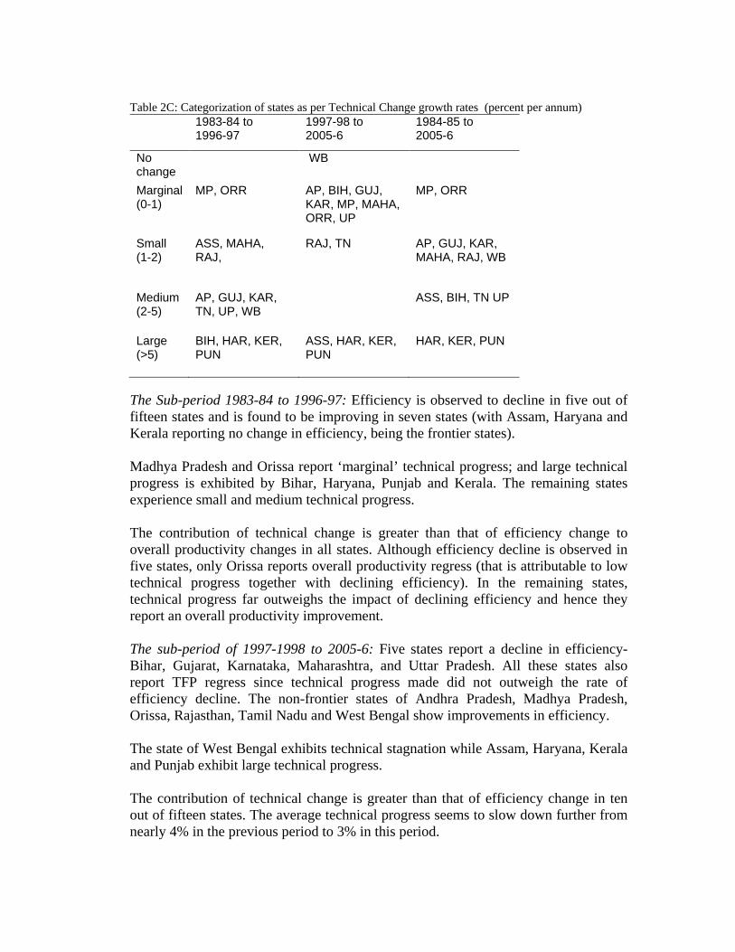
Table 2C: Categorization of states as per Technical Change growth rates (percent per annum) 1983-84 to

1996-97 1997-98 to 2005-6

1984-85 to 2005-6

No change

WB

Marginal (0-1)

MP, ORR AP, BIH, GUJ, KAR, MP, MAHA, ORR, UP

MP, ORR

Small (1-2)

ASS, MAHA, RAJ,

RAJ, TN AP, GUJ, KAR, MAHA, RAJ, WB

Medium (2-5)

AP, GUJ, KAR, TN, UP, WB

ASS, BIH, TN UP

Large (>5)

BIH, HAR, KER, PUN

ASS, HAR, KER, PUN

HAR, KER, PUN

The Sub-period 1983-84 to 1996-97: Efficiency is observed to decline in five out of fifteen states and is found to be improving in seven states (with Assam, Haryana and Kerala reporting no change in efficiency, being the frontier states). Madhya Pradesh and Orissa report ‘marginal’ technical progress; and large technical progress is exhibited by Bihar, Haryana, Punjab and Kerala. The remaining states experience small and medium technical progress. The contribution of technical change is greater than that of efficiency change to overall productivity changes in all states. Although efficiency decline is observed in five states, only Orissa reports overall productivity regress (that is attributable to low technical progress together with declining efficiency). In the remaining states, technical progress far outweighs the impact of declining efficiency and hence they report an overall productivity improvement. The sub-period of 1997-1998 to 2005-6: Five states report a decline in efficiency- Bihar, Gujarat, Karnataka, Maharashtra, and Uttar Pradesh. All these states also report TFP regress since technical progress made did not outweigh the rate of efficiency decline. The non-frontier states of Andhra Pradesh, Madhya Pradesh, Orissa, Rajasthan, Tamil Nadu and West Bengal show improvements in efficiency. The state of West Bengal exhibits technical stagnation while Assam, Haryana, Kerala and Punjab exhibit large technical progress. The contribution of technical change is greater than that of efficiency change in ten out of fifteen states. The average technical progress seems to slow down further from nearly 4% in the previous period to 3% in this period.

Taking the average performance of all the fifteen states on the technical efficiency front, efficiency decline is observed in the first sub-period as well as overall time period, while being almost stagnant in second sub-period (Table 2A). Table 3 reports the states categorized as per their technical efficiency scores. The efficiency of five states- Madhya Pradesh, Uttar Pradesh, Andhra Pradesh, Karnataka, Maharashtra - is less than fifty percent implying even with existing technology, better utilization of resources would result in huge increases in output. The efficiency performance of Bihar has shown a declining trend over time- from around 70% during 1983-84 to 1996-97 to less than 50% during 1997-98 to 2005-6. The efficiency scores of Gujarat and West Bengal lie in the range 50-80% for all the time periods. The state of Rajasthan exhibits an improvement in efficiency score from 50-80% in the first sub-period to more than 80% in the second sub-period. Punjab and Assam operate beyond 80% of efficiency level, attaining full technical efficiency in several sub-periods. The state of Orissa also reports more-than-80% technical efficiency. Haryana remains technically efficient in all the sub-periods; while Kerala’s efficiency falls little below 100% during 1997-98 to 2005-6 (otherwise remaining fully efficient in first sub period). Table 3: Categorization of states as per Technical Efficiency Scores (percent) Less than fully Technically efficient Fully technically

efficient 0-30 30-50 50-80 80-100 100 1983-84 to 1996-97

MP AP, KAR, MAHA, UP

BIH, GUJ, RAJ, WB

ORR, PUN, TN, ASS

HAR, KER

1997-98 to 2005-6

UP AP, BIH, KAR, MP, MAHA

GUJ, WB ASS, KER, ORR, PUN, RAJ, TN

HAR

1983-84 to 2005-6

MP, UP

AP, KAR, MAHA

BIH,GUJ, RAJ, WB

ASS,KER, ORR, PUN, TN

HAR

V.2 TFP Results (excluding Bihar and Kerala) When Malmquist TFP index is computed for thirteen states excluding Bihar and Kerala, the TFP growth, efficiency change and technical change are all computed with reference to a new frontier constructed for these states which would alter since one of the frontier states- Kerala- has been dropped. Hence results are liable to change. A comparison of the productivity results for thirteen states (excluding Bihar and Kerala) and fifteen states (including Bihar and Kerala) is presented in Table 4. The columns under ‘A’ are TFP growth rates excluding Bihar and Kerala and those under ‘B’ are computed including Bihar and Kerala (the latter discussed in previous sub-section). When correlation is computed across the two series of TFP growth rates for all the states, it is found that the two are highly correlated (correlation coefficient

being more than 0.95) with the exception of states of Karnataka and West Bengal (with correlation coefficient being 0.81 and 0.87 respectively). In most of the states, the direction of TFP change is the same although there is a change in the magnitude. A change in direction of productivity change is noted for Gujarat- in sub period 1 and overall time period when TFP improvement (computations including Bihar and Kerala- column B) gets replaced by productivity regress (computations excluding Bihar and Kerala- column A); and Karnataka in second sub-period when TFP regress (column B) is replaced by productivity improvement (column A). Table 4: A comparison of TFP growth rates including and excluding Bihar and Kerala 1983-84 to 1996-97 1997-98 to 2005-6 1983-84 to 2005-6 Correlation A B A B A B AP 1.36 1.33 3.40 2.23 2.19 1.69 0.98 ASS 1.43 1.84 8.97 8.58 4.45 4.54 1.00 BIH 3.08 -0.84 1.46 GUJ -0.30 2.93 -2.62 -2.93 -1.25 0.49 0.95 HAR 9.18 8.36 10.21 8.34 9.60 8.35 0.96 KAR 2.56 2.99 3.21 -0.40 2.83 1.59 0.81 KER 12.56 8.11 10.72 MAHA 3.47 3.71 -1.43 -2.44 1.44 1.15 0.97 MP 0.42 0.45 0.91 0.90 0.62 0.63 1.00 ORR -2.33 -2.33 2.21 2.15 -0.50 -0.52 1.00 PUN 8.94 8.00 17.65 14.64 12.43 10.67 0.96 RAJ 1.50 1.37 2.71 2.71 2.00 1.92 1.00 TN 7.11 6.82 6.30 3.66 6.78 5.52 0.98 UP 2.97 2.97 -0.65 -0.65 1.48 1.47 1.00 WB 1.24 2.95 2.83 2.33 1.89 2.70 0.87 Mean 2.84 3.74 4.01 2.99 3.32 3.43 0.91

Section VI: Contemporaneous and Sequential Malmquist TFP Index- A Comparison of Results

The changes in TFP and its decomposition as obtained for fifteen states from the two alternate ways of frontier construction- contemporaneous and sequential- are hereby examined. As mentioned in Section III, Malmquist TFP index, when estimated using the notion of contemporaneous technology, gives rise to two biases- over-estimation of efficiency change and under-estimation of technical change. Table 5 lays down the growth rates of TFP, technical efficiency and technical change computed using the two notions for the overall time period 1983-84 to 2005-6. The mean TFP growth is found to be 1.6% and 3.4% per annum under contemporaneous and sequential technology respectively. In comparison to sequential approach, the technical efficiency change computed under contemporaneous approach is observed to be over-reported for all states (except Tamil Nadu) as well as on the average- mean technical efficiency growth rate being 0.41% p.a. under contemporaneous technology while it is estimated as -0.11% p.a. under sequential technology.

Table 5: TFP growth, Technical Efficiency Change and Technical Change (1983-84 to 2005-6) (percent per annum) State Contemporaneous Technology Sequential Technology TEC TC TFP TEC TC TFP

AP 0.56 0.58 1.15 -0.11 1.80 1.69 ASS 0.00 -0.87 -0.87 0.00 4.54 4.54 BIH -0.93 2.15 1.20 -1.96 3.50 1.46 GUJ -0.70 0.50 -0.20 -1.32 1.83 0.49 HAR 0.00 3.71 3.71 0.00 8.35 8.35 KAR 0.68 1.13 1.82 -0.17 1.77 1.59 KER 0.00 3.97 3.97 0.00 10.72 10.72 MAHA 0.96 -1.26 -0.30 -0.10 1.26 1.15 MP 0.50 0.72 1.21 -0.01 0.66 0.63 ORR 0.00 -2.55 -2.55 -0.89 0.37 -0.52 PUN 0.00 8.47 8.47 0.01 10.68 10.67 RAJ 0.98 0.59 1.58 0.42 1.48 1.92 TN 2.25 0.23 2.49 2.25 3.20 5.52 UP 0.07 1.23 1.30 -1.00 2.49 1.47 WB 1.63 0.46 2.10 1.24 1.43 2.70 Mean 0.41 1.23 1.64 -0.11 3.55 3.43

When the entire time–period is considered, technical regress is reported in two frontier states- Assam and Orissa (Table 5). However it is useful to look at technical regress in frontier countries on year-to-year basis (see Table 6). Table 6: Technical Regress in the states lying on the frontier in computation of contemporaneous Malmquist TFP index Frontier States Number of years for which technical regress is

reported Always on the frontier Assam 13 Haryana 9 Kerala 7

For most of the years Tamil Nadu 10

For few years Punjab 5 Rajasthan 3 The fact that there might be a fall in the use of one or more inputs causes technical regress under contemporaneous frontier. For states like Punjab, Haryana and Tamil Nadu- well known for adoption of new technology- a rise in use of fertilizers, tractors and irrigation is accompanied by a decline in inputs like livestock over the years.

Assam, apart from reduced use of livestock over the years, also witnessed a decline in the irrigation input since 2000 onwards due to large-scale devastation caused by floods. Kerala, another frontier state, reports a decline in the use of one of the inputs- livestock after 1996. The factors that have attributed to this decline are “scarcity of cheap and quality fodder, rapid increase in the price of feed and feed ingredients, inflow of cheap and low quality livestock products from neighbouring states, indiscriminate slaughter of animals, under exploitation of production potential of animals, non availability of good germplasm and threat from contagious diseases like FMD etc”14

14 http://www.livestockkerala.org/livescen.htm

. The state of Rajasthan has witnessed a decline in gross cropped area and livestock in few years. Such declines in usage of inputs result in frontier receding inward causing biased TFP estimates. Hence there arises the need for constructing frontier using sequential technology. Summing up It is a matter of serious concern that efficiency decline is observed in almost fifty percent of the states. This implies huge potential increase in production even with existing technology. Some of these states do not report overall productivity regress only due to the fact that technical progress outweighs the impact of decline in efficiency. The technical stagnation and near-stagnation is observed in most of the states. Demand for food would continue to rise and food supply has to keep pace in order to avoid shortages. This requires production to increase manifold. Since net area under cultivation has almost exhausted, productivity levels have to increase by leaps and bounds. It is necessary to reverse the efficiency decline that is exhibited by many states and achieve a faster and larger scale of diffusion of technical innovations across states.

References: Ahmad S. (1966), “On the theory of induced innovation”, Economic Journal, Vol. 76, p344-357. Alene Arega D. (2009), “Productivity Growth and the Effects of Reasearch and Development in African Agriculture”, Contributed paper prepared for the presentation at the International Association of Agricultural Economists Conferenvce, Beijing, China, August 16-22. Arnade C. (1998), “Using a programming approachto measure international agricultural efficiency and productivity”, Journal of Agricultural Economics, Vol. 49, p67-84. Alcantara Reinaldo, Prato Anthony A. (1973), “Returns to Scale and Input Elasticities for Sugarcane: The case of Sao Paulo, Brazil”, American Journal of Agricultural Economics, November 1973, pp577-583. Balakrishnan Pulapre (2010), “Economic Growth in India- History and Prospect”, Oxford University Press. Bhattacharya B. B, Sakthivel S (2004), “Regional Growth and Disparity in India- Comparison of Pre- and Post-Reform Decades”, Economic and Political Weekly March 6, 2004 , pp1071-1077. Bhushan Surya (2005), “Total Factor Productivity Growth of Wheat in India: A Malmquist Approach”, Indian Journal of Agricultural Economics, Vol 60, No.1 Jan-March 2005. Binswanger Hans P., Ruttan Vernon W. (1978), “Induced Innovation: Technology, Institutions and Development”, The John Hopkins University Press, Baltomore and London. Bosworth Barry, Collins Susan M.(2007), “Accounting for Growth: Comparing China and India”, Working Paper 12943, National Bureau of Economic Research. Carlaw Kenneth I; Mawson Peter; McLellan Nathan, “Productivity Measurement: Alternative Approaches and Estimates”, June 2003, New Zealand Treasury Working Paper 03/12. Caves D.W., Christensen L.R., Diewert W.E. (1982), “The economic theory of index numbers and the measurement of input, output and productivity”, Econometrica 50, p 1393-1414. Chand Ramesh, Kumar Praduman, Kumar Sant (2011), “Total Factor Productivity and Contribution of Research Investment to Agricultural Growth in India”, National

Council for Agricultural Economic and Policy Research, Policy Paper 25, March 2011. Coelli Tim, Rahman Sanzidur, Thirtle Colin (2003), "A Stochastic Frontier Approach to Total Factor Productivity measurement in Bangladesh crop agriculture”, Journal of International Development, 15, 321-333. Coelli Tim J., Rao D.S. Prasada (2003), “Total Factor Productivity Growth in Agriculture: A Malmquist Index Analysis of 93 Countries1980-2000”, Centre for Efficiency and Productivity Analysis, Working Paper Series, No. 02/2003, School of Economics, University of Queensland Australia. Coelli Tim J., Rao D.S. Prasada, O’Donnell Christopher J., Battesse George E. (2005), “An Introduction to Efficiency and Productivity Analysis (Second Edition)”, Springer. Coelli Tim, “A Data Envelopment Analysis (Computer) Program”, Centre for Efficiency and Productivity Analysis, Department of Econometrics, University of New England, Australia. Fan Shenggen, Hazell Peter, and Thorat Sukhadeo (1998), “Government Spending, Growth and Poverty: An Analysis of Interlinkages in Rural India”, EPTD Discussion Paper No. 33, Environment and Production Technology Division, International Food Policy Research Institute, USA. Forstner Helmut, Isaksson Anders, Ng Thiam Hee (2001), “Growth in Least Developed Countries- An Empirical Analysis of Productivity Change, 1970 – 1992”, SIN WORKING PAPER SERIES, Working Paper No 1, November 2001. Forstner Helmut and Isaksson Anders (2002), “Productivity, Technology, and Efficiency: An analysis of the world technology frontier when memory is infinite”, SIN Working Paper Series, Working Paper no. 7, February 2002, Statistics and Information Networks branch of UNIDO. Fulginiti L. E., and Perrin R.K. (1993), “Prices and Productivity in Agriculture”, Review of Economics and Statistics, Vol. 75, p471-482. Fulginiti L. E., and Perrin R.K. (1997), “LDC Agriculture: Non-parametric Malmquist Productivity Indices”, Journal of Development Economics, Vol.53, p373-390. Fulginiti L. E., and Perrin R.K. (1998), “Agricultural Productivity in Developing Countries”, Agricultural Economics, Vol. 19, p45-51. Grifell-Tatje E, Lovell C. A. K. (1995), “A note on the Malmquist productivity index”, Economics Letters, Vol. 47, p169-175.

Government of India, Fertilizer Statistics, various issues. Goyal S.K., Suhag K.S. (2003), “Estimation of Technical Efficiency on Wheat Farms in Northern India- A Panel Data Analysis”, Paper presented at International Farm Management Congress- ‘Farming at the Edge’. Hayami Yujiro, Ruttan Vernon W. (1985), “Agricultural Development: An International Perspective”, The Johns Hopkins University Press, Baltimore and London. http://www.livestockkerala.org/livescen.htm Isaksson Anders (2007), “World Productivity Database: A Technical Description”, Research and Statistics Branch, staff working paper 10/2007, December 2007, United Nations Industrial Development Organization. Isaksson Anders and Ng Thiam Hee (2006), “Determinants of Productivity: Cross-Country Analysis and Country Case Studies”, Staff working paper 01/2006, Research and Statistics Branch, UNIDO, October 2006. Kawagoe T., Hayami Y. (1985), “An intercountry comparison of agricultural production efficiency”, American journal of Agricultural Economics, Vol. 67, p 87-92. Kawagoe T., Hayami Y., Ruttan V. (1985), “The intercountry agricultural production function and productivity differences among countries”, Journal of Development Economics, Vol. 19, p113-32. Khaldi Nabil (1975), “Education and Allocative Efficiency in U.S. Agriculture”, American Journal of Agricultural Economics, November 1975, pp650-657. Kudaligama Viveka P. and Yanagida John F. (2000), “A Comparison of Intercountry Agricultural Production Functions: A Frontier Function Approach”, Journal of Economic Development Volume 25, Number 1, June 2000, p57-73. Kumar Praduman, Mittal Surabhi (2006), “Agricultural Productivity Trends in India: Sustainability Issues”, Agricultural Economics Research Review Vol. 19 (Conference No.) pp 71-88. Kumar Praduman, Rosegrant Mark W (1994), “Productivity and Sources of Growth for Rice in India”, Economic and Political Weekly December 31, 1994, p A-183 to A-188.

Lao L., Yotopoulas P. (1989), “The meta production function approach to technological change in world agriculture”, Journal of Development Economics, Vol. 31, p 241-269. Lopez E. Ramon (1980), “The Structure of Production and the Derived Demand for Inputs in Canadian Agriculture”, American Journal of Agricultural Economics, February 1980, pp38-45. Mawson Peter, Carlaw Kenneth I and McLellan Nathan (2003), “Productivity measurement: Alternative approaches and estimates”, New Zealand Treasury, Working Paper 03/12, June 2003. Mukherjee, Anit, and Y. Kuroda. (2001) “Effect of Rural Nonfarm Employment and Infrastructure on Agricultural Productivity: Evidence from India.” Discussion Paper No. 938. University of Tsukuba, Ibaraki, Japan. http://infoshako.sk.tsukuba.ac.jp/~databank/thesis/2003/a2003kuroda.pdf (Accessed on 17th May, 2011) Murgai Rinku (1999), “The Green Revolution and the Productivity Paradox- Evidence from the Indian Punjab”, Policy Research Working Paper 2234, The World Bank Development Research Group, Rural Development, November 1999. National Sample Survey Organization, National Sample Survey Reports, Ministry of Statistics and Programme Implementation, Government of India, various issues. Nayak Pulin B, Goldar Bishwanath, Agarwal Pradeep (ed) (2010), “India’s Economy and Growth- Essays in Honor of V.K.R.V. Rao”, Sage Publications. Nin Alejandro, Arndt Channing, Preckel Paul V. (2003), “Is agricultural productivity in developing countries really shrinking? New evidence using a modified nonparametric approach”, Journal of Development Economics 71, p 395-415. Rahman Sanzidur (2004), “Regional Productivity and Convergence in Bangladesh Agriculture”, Paper presented at the Annual Meeting of the American Agricultural Economics Association held in Aug 1-4, 2004, Project MUSE Scholarly Journals Online. Rao N. Chandrashekhara (2005), “Total Factor Productivity in Andhra Pradesh Agriculture”, American Economics Research Review, Vol 18, Jan-June 2005, p1-19. Ray Subhash C. (2004), “Data Envelopment Analysis: Theory and Techniques for Economics and Operations Research”, Cambridge University Press. Rogers Mark (1998), “The Definition and Measurement of Productivity”, Melbourne Institute Working Paper No. 9/98, Melbourne Institute of Applied Economic and Social Research, The University of Melbourne.

Rosegrant Mark W, Evenson (1992), “The rate of growth of Total Factor Productivity in Indian crop sector 1957-1985”, American Journal of Agricultural Economics, August 1992, 757-763. Statistical Abstract, India and of individual states, various issues. Trueblood M.A. (1996), “An intercountry comparison of agricultural efficiency and productivity”, Ph.D dissertation, University of Minnesota. Tulkens, H. and Eeckaut P. Vanden (1995), "Non-Parametric Efficiency, Progress and Regress Measures For Panel Data: Methodological Aspects," European Journal of Operations Research 80, pp. 474-99. Wan Guang H., Cheng Enjiang (2001), “Effects of land fragmentation and returns to scale in Chinese farming sector”, Applied Economics, Vol 33, pp183-194.

Appendix 1: Data envelopment Approach to computing Sequential Malmquist TFP Index

The output oriented constant returns to scale DEA model for M outputs and K inputs can be written as:

maxφ,λ φ, s.t. -φyi + Yλ ≥ 0,

xi - Xλ ≥ 0, λ ≥ 0, (1)

where yi is a M×1 vector of output quantities for the i-th state; xi is a K×1 vector of input quantities for the i-th state; Y is a M×N matrix of output quantities for all N states; X is a K×N matrix of input quantities for all N states; λ is a N×1 vector of weights; and φ is a scalar.

If there is only one output (as in the present case), the DEA model can be re-written as:

maxφ,λ φ, s.t. -φyi + Yλ ≥ 0,

xi - Xλ ≥ 0, λ ≥ 0, (1)

where y is the output quantity for the i-th state; xi is a K×1 vector of input quantities for the i-th state; Y is a 1×N matrix of output quantities for all N states; X is a K×N matrix of input quantities for all N states; λ is a N×1 vector of weights; and φ is a scalar.

Four distance functions need to be calculated to measure the TFP change between two time periods that requires solving of following four linear programming problems.

[dot(xt,yt)]-1 = max ф,λ ф ,

st - фyit + Σr=1to t Σn=1to N λrn yr

n≥ 0 xit - Σr=1to t Σn=1to N λr

k xrn ≥ 0,

λrk ≥ 0.

[dos(xs,ys)]-1 = max ф,λ ф ,

st - фyis + Σr=1to s Σn=1to N λrn yr

n≥ 0 xis - Σr=1to s Σn=1to N λr

k xrn ≥ 0,

λrk ≥ 0.

[do

t(xs,ys)]-1 = max ф,λ ф , st - фyis + Σr=1to t Σn=1to N λr

n yrn≥ 0

xis - Σr=1to t Σn=1to N λrk xr

n ≥ 0, λr

k ≥ 0.

[dos(xt,yt)]-1 = max ф,λ ф ,

st - фyit + Σr=1to s Σn=1to N λrn yr

n≥ 0 xit - Σr=1to s Σn=1to N λr

k xrn ≥ 0,

λrk ≥ 0.

Appendix 2

Table A1(a): Malmquist TFP Indices computed using sequential technology (including Bihar and Kerala) AP ASS BIH GUJ HAR KAR KER MAHA MP ORR PUN RAJ TN UP WB

1985 1.09 1.125 1.271 1.17 1.129 1.108 1.203 1.151 1.029 0.828 1.076 0.915 1.638 1.214 1.263 1986 0.941 1.089 1.131 0.762 1.087 1.033 1.068 0.902 0.942 1.171 0.987 0.976 1.084 0.852 1.153 1987 0.928 0.951 1.223 1.171 1.133 1.012 1.059 0.903 1.014 0.919 1.061 1.237 1.071 1.435 1.008 1988 1.062 1.055 0.668 0.751 1.323 0.894 1.062 1.219 1.041 0.936 1.562 0.602 0.989 1.178 0.94 1989 1.171 0.949 1.416 1.512 1.091 0.95 1.096 0.921 0.998 1.22 0.805 1.855 1.059 0.799 1.095 1990 0.949 1.049 0.839 1.034 1.132 1.16 1.004 1.234 0.99 1.058 1.344 0.768 1.041 1.037 0.872 1991 1.111 0.966 1.16 0.863 1.043 0.96 1.155 0.944 0.855 0.777 0.937 1.541 1.05 1.015 1.047 1992 0.993 0.993 0.945 0.93 1.051 1.13 1.047 0.931 1.115 1.191 1.265 0.645 1.039 1.175 0.903 1993 1.059 1.014 0.944 1.322 1.029 1.144 1.164 1.213 1.049 0.89 0.976 1.234 1.146 0.891 1.136 1994 0.957 0.994 1.08 0.801 1.029 0.973 1.185 0.909 1.077 1.001 0.967 0.674 0.946 1.015 0.887 1995 0.956 1.02 0.999 1.147 1.04 0.905 1.219 1.05 0.835 0.885 1.053 1.402 1.183 0.975 1.145 1996 1.057 1.003 0.761 1.113 1.007 1.088 1.225 1.199 1.131 1.153 0.982 0.845 0.994 0.961 0.842 1997 0.935 1.047 1.252 1.094 1.028 1.081 1.175 1.013 1.031 0.813 1.235 1.286 0.818 0.999 1.206 1998 0.974 1.001 0.693 0.853 1.018 0.883 1.041 0.713 0.906 1.218 0.939 1.035 1.175 0.956 0.947 1999 1.23 0.958 1.182 1.045 1.022 1.057 1.086 1.205 1.174 0.96 1.003 1.076 1.089 1 0.959 2000 1.006 1.048 0.868 0.844 1.202 1.118 1.121 1.151 1.049 0.895 1.226 0.871 1.058 0.925 1.014 2001 1.134 1.594 1.223 0.815 1.011 1.154 0.918 0.831 1.177 1.018 1.088 0.816 0.809 1.002 1.079 2002 0.919 1.035 0.885 1.45 1.083 0.872 1.068 1.148 0.929 1.17 1.073 1.646 1.01 1.032 1.129 2003 0.879 1.021 1.337 0.692 1.088 0.91 1.098 1.043 1.186 1.111 0.996 0.575 0.809 1.16 0.911 2004 0.963 1.007 0.754 1.685 1.154 0.75 1.128 0.928 0.79 0.786 1.415 1.916 0.881 0.78 1.082 2005 1.185 1.155 1.281 0.879 1.15 1.506 1.142 1.026 1.032 1.209 1.412 0.946 1.395 1.271 0.982 2006 0.968 1.065 0.933 0.84 1.04 0.894 1.148 0.855 0.919 0.92 1.275 0.937 1.257 0.897 1.133

Table A1(b): Technical Change Component of Malmquist TFP indices computed using sequential technology (including Bihar and Kerala) AP ASS BIH GUJ HAR KAR KER MAHA MP ORR PUN RAJ TN UP WB mean

1985 1.022 1.125 1.144 1.037 1.129 1.075 1.203 1.041 1.01 1.001 1.1 1.033 1.003 1.003 1.083 1.066 1986 1.083 1.089 1.136 1.054 1.087 1.145 1.068 1.134 1.059 1.023 1.027 1.004 1.084 1.061 1.148 1.079 1987 1.018 1 1.092 1.051 1.133 1.017 1.059 1.003 1 1 1.079 1.036 1.071 1.113 1.051 1.047 1988 1.003 1.003 1.004 1.032 1.323 1.006 1.062 1 1 1 1.444 1.064 1.001 1.186 1 1.068 1989 1.02 1 1 1.006 1.091 1.012 1.096 1.002 1.001 1.001 1.069 1 1.046 1.002 1 1.023 1990 1.029 1 1.003 1.03 1.132 1.003 1.004 1.005 1.002 1.051 1.1 1.027 1.041 1.001 1 1.028 1991 1.012 1 1.159 1.016 1.043 1.04 1.155 1.004 1.004 1 1.043 1.001 1.05 1.028 1.025 1.038 1992 1.041 1.001 1.01 1.015 1.051 1.002 1.047 1.002 1.001 1 1.046 1 1.039 1 1.003 1.017 1993 1.069 1.002 1.022 1.053 1.029 1.004 1.164 1.019 1.019 1.002 1.02 1 1.146 1.108 1.008 1.043 1994 1 1 1 1 1.029 1 1.185 1 1 1 1.006 1 1 1 1 1.014 1995 1.053 1 1.039 1.045 1.04 1.004 1.219 1.021 1.018 1.002 1 1 1.119 1.015 1.004 1.037 1996 1 1 1.191 1.01 1.007 1.076 1.225 1 1.001 1 1.086 1 1 1 1 1.037 1997 1.002 1.028 1 1.002 1.028 1.001 1.175 1.02 1.001 1.001 1.082 1 1 1 1.005 1.022 1998 1 1.001 1 1 1.018 1 1.041 1 1 1 1 1 1 1 1 1.004 1999 1.012 1.001 1 1.014 1.022 1.002 1.086 1.004 1.008 1 1.003 1 1.041 1 1 1.013 2000 1.034 1.003 1 1.032 1.202 1.01 1.121 1.007 1.012 1.001 1.227 1 1.058 1.042 1 1.048 2001 1 1.594 1 1 1.011 1 1 1 1 1 1.022 1 1 1 1 1.034 2002 1.001 1.035 1 1.001 1.083 1.003 1 1.018 1 1 1.073 1.066 1 1.001 1 1.018 2003 1 1.021 1 1 1.088 1 1.077 1 1 1 1.096 1 1 1.012 1 1.019 2004 1 1.007 1 1 1.154 1 1.128 1 1.007 1 1.286 1.102 1.001 1 1 1.043 2005 1 1.155 1 1.006 1.15 1.002 1.142 1.002 1.004 1 1.412 1 1.003 1 1 1.053 2006 1.002 1.065 1.007 1.002 1.04 1 1.148 1.003 1 1 1.275 1 1.018 1 1 1.035

Table A1(c): Technical Efficiency Change Component of Malmquist TFP indices computed using sequential technology (including Bihar and Kerala) AP ASS BIH GUJ HAR KAR KER MAHA MP ORR PUN RAJ TN UP WB mean 1985 1.066 1 1.111 1.128 1 1.031 1 1.106 1.018 0.827 0.978 0.886 1.633 1.21 1.167 1.065 1986 0.869 1 0.995 0.723 1 0.902 1 0.795 0.89 1.144 0.961 0.972 1 0.804 1.004 0.931 1987 0.912 0.951 1.12 1.114 1 0.995 1 0.9 1.014 0.919 0.984 1.193 1 1.289 0.959 1.018 1988 1.059 1.052 0.666 0.728 1 0.889 1 1.219 1.041 0.936 1.082 0.565 0.988 0.994 0.939 0.927 1989 1.148 0.949 1.416 1.503 1 0.939 1 0.92 0.997 1.219 0.754 1.855 1.012 0.797 1.095 1.076 1990 0.922 1.049 0.836 1.003 1 1.157 1 1.227 0.988 1.007 1.221 0.748 1 1.035 0.871 0.996 1991 1.098 0.966 1.001 0.849 1 0.924 1 0.94 0.852 0.777 0.898 1.539 1 0.988 1.022 0.979 1992 0.953 0.992 0.936 0.916 1 1.127 1 0.929 1.114 1.19 1.209 0.645 1 1.175 0.901 0.995 1993 0.991 1.012 0.924 1.256 1 1.14 1 1.191 1.03 0.888 0.957 1.234 1 0.804 1.127 1.029 1994 0.957 0.994 1.08 0.801 1 0.973 1 0.909 1.077 1.001 0.962 0.674 0.946 1.015 0.887 0.946 1995 0.907 1.02 0.962 1.098 1 0.902 1 1.029 0.821 0.883 1.053 1.402 1.057 0.961 1.139 1.008 1996 1.057 1.003 0.639 1.102 1 1.011 1 1.199 1.13 1.153 0.905 0.845 0.994 0.961 0.842 0.979 1997 0.933 1.018 1.252 1.092 1 1.08 1 0.993 1.031 0.812 1.142 1.286 0.818 0.999 1.2 1.035 1998 0.974 1 0.693 0.853 1 0.883 1 0.713 0.906 1.218 0.939 1.035 1.175 0.956 0.947 0.943 1999 1.215 0.957 1.182 1.031 1 1.055 1 1.201 1.166 0.96 1 1.076 1.047 1 0.959 1.053 2000 0.973 1.045 0.868 0.818 1 1.107 1 1.143 1.036 0.895 1 0.871 1 0.887 1.014 0.973 2001 1.134 1 1.223 0.815 1 1.154 0.918 0.831 1.177 1.018 1.065 0.816 0.809 1.002 1.079 0.993 2002 0.918 1 0.885 1.448 1 0.869 1.068 1.127 0.929 1.17 1 1.544 1.01 1.031 1.129 1.061 2003 0.879 1 1.337 0.692 1 0.91 1.02 1.043 1.186 1.111 0.909 0.575 0.809 1.146 0.911 0.949 2004 0.963 1 0.754 1.685 1 0.75 1 0.928 0.785 0.786 1.1 1.738 0.88 0.78 1.082 0.981 2005 1.185 1 1.281 0.874 1 1.503 1 1.025 1.028 1.209 1 0.946 1.391 1.271 0.982 1.100 2006 0.966 1 0.927 0.838 1 0.893 1 0.852 0.919 0.92 1 0.937 1.235 0.897 1.133 0.963

Table A2(a): Malmquist TFP Indices computed using sequential technology (excluding Bihar and Kerala) AP ASS GUJ HAR KAR MAHA MP ORR PUN RAJ TN UP WB mean

1985 1.09 1.125 0.76 1.128 0.999 1.117 1.029 0.827 1.076 0.916 1.638 1.213 1.675 1.096 1986 0.941 1.089 0.762 1.105 1.003 0.903 0.942 1.171 0.997 0.976 1.084 0.853 1.131 0.990 1987 0.934 0.951 1.211 1.16 1.014 0.905 1.009 0.92 1.051 1.267 1.076 1.434 1.015 1.063 1988 1.062 1.005 0.751 1.322 0.946 1.218 1.041 0.936 1.536 0.601 0.989 1.179 0.914 1.012 1989 1.171 0.948 1.511 1.123 0.998 0.967 0.998 1.22 0.859 1.855 1.059 0.799 1.041 1.091 1990 0.949 1.05 1.034 1.132 1.103 1.176 0.99 1.058 1.317 0.768 1.041 1.037 0.707 1.016 1991 1.106 0.965 0.863 1.067 0.86 0.973 0.855 0.777 0.973 1.541 1.051 1.015 0.867 0.979 1992 0.993 0.993 0.929 1.05 1.159 0.899 1.115 1.191 1.223 0.645 1.044 1.175 0.896 1.011 1993 1.058 1.014 1.322 1.029 1.139 1.214 1.049 0.89 1.004 1.234 1.146 0.891 1.136 1.080 1994 0.956 0.993 0.801 1.028 1.035 0.91 1.077 1.001 1.042 0.674 0.973 1.015 0.887 0.946 1995 0.957 1.019 1.168 1.042 0.975 1.05 0.836 0.885 1.081 1.402 1.167 0.975 1.145 1.045 1996 1.056 1.009 1.077 1.008 1.008 1.199 1.13 1.153 1.008 0.84 0.994 0.961 0.842 1.017 1997 0.939 1.04 1.095 1.035 1.137 1.013 1.032 0.813 1.146 1.286 0.826 0.999 1.203 1.035 1998 0.97 1.004 0.876 1.018 0.932 0.714 0.906 1.218 0.96 1.035 1.179 0.956 0.947 0.970 1999 1.248 0.969 1.053 1.041 1.235 1.291 1.175 0.96 1.061 1.076 1.132 1 0.959 1.087 2000 1.006 1.053 0.838 1.203 1.026 1.092 1.049 0.896 1.175 0.871 1.058 0.925 1.017 1.011 2001 1.144 1.604 0.815 1.048 1.126 0.832 1.177 1.018 1.085 0.816 0.838 1.002 1.077 1.027 2002 0.915 1.035 1.45 1.084 0.862 1.147 0.928 1.171 1.062 1.646 1.075 1.032 1.129 1.101 2003 0.875 1.029 0.693 1.088 0.839 1.043 1.187 1.11 1.009 0.575 0.774 1.16 0.911 0.927 2004 0.963 1.007 1.685 1.252 0.88 0.927 0.79 0.786 1.567 1.916 0.999 0.78 1.085 1.077 2005 1.185 1.153 0.879 1.145 1.405 1.027 1.032 1.212 1.46 0.946 1.485 1.271 0.992 1.154 2006 1.061 1.066 0.84 1.062 1.118 0.921 0.919 0.922 1.357 0.937 1.186 0.897 1.167 1.026

Mean 1.022 1.044 0.987 1.096 1.028 1.014 1.006 0.995 1.124 1.020 1.068 1.015 1.019 1.033

Table A2(b): Technical Change Component of Malmquist TFP indices computed using sequential technology (excluding Bihar and Kerala) AP ASS GUJ HAR KAR MAHA MP ORR PUN RAJ TN UP WB mean

1985 1.022 1.125 1.119 1.128 1.04 1.036 1.01 1.001 1.1 1.033 1.003 1.003 1.038 1.050 1986 1.083 1.089 1.055 1.105 1.107 1.135 1.059 1.023 1.037 1.004 1.084 1.061 1.102 1.072 1987 1.059 1 1.086 1.16 1.32 1.055 1.005 1 1.216 1.062 1.076 1.113 2.064 1.147 1988 1.003 1.003 1.031 1.322 1 1 1 1 1.427 1.064 1.001 1.185 1 1.072 1989 1.02 1 1.006 1.123 1.009 1.004 1.001 1.001 1.109 1 1.046 1.002 1.002 1.024 1990 1.029 1 1.03 1.132 1 1.003 1.002 1.051 1.074 1.027 1.041 1.001 1 1.029 1991 1.008 1 1.016 1.067 1 1.002 1.004 1 1.098 1.001 1.051 1.028 1 1.021 1992 1.041 1 1.015 1.05 1 1.001 1.001 1 1.031 1 1.044 1 1.002 1.014 1993 1.069 1 1.053 1.029 1 1.019 1.019 1.002 1.025 1 1.146 1.108 1 1.035 1994 1 1 1 1.028 1.001 1 1 1 1.021 1 1 1 1 1.004 1995 1.053 1 1.038 1.042 1.008 1.021 1.018 1.002 1.081 1 1.135 1.015 1.004 1.031 1996 1 1 1 1.008 1 1 1 1 1.008 1 1 1 1 1.001 1997 1.003 1.028 1.003 1.035 1.01 1.019 1.001 1.001 1.146 1 1.001 1 1.003 1.019 1998 1 1.004 1 1.018 1 1 1 1 1 1 1 1 1 1.002 1999 1.019 1 1.045 1.041 1.036 1.001 1.008 1 1.019 1 1.094 1 1 1.020 2000 1.041 1.02 1.032 1.203 1.039 1.015 1.012 1.001 1.175 1 1.058 1.042 1.001 1.047 2001 1 1.604 1 1.048 1.031 1.011 1 1 1.085 1 1 1 1 1.051 2002 1 1.035 1.001 1.084 1.011 1.018 1 1 1.062 1.066 1 1.001 1 1.021 2003 1 1.029 1 1.088 1.028 1 1 1 1.042 1 1 1.011 1 1.015 2004 1 1.007 1 1.252 1.009 1 1.007 1 1.518 1.102 1.007 1 1 1.061 2005 1 1.153 1.006 1.145 1.002 1.002 1.004 1 1.46 1 1.026 1 1 1.055 2006 1.007 1.066 1.001 1.062 1.025 1.003 1 1 1.357 1 1.186 1 1 1.050

Table A2(c): Technical Efficiency Change Component of Malmquist TFP indices computed using sequential technology (excluding Bihar and Kerala) AP ASS GUJ HAR KAR MAHA MP ORR PUN RAJ TN UP WB mean

1985 1.066 1 0.679 1 0.961 1.079 1.019 0.827 0.978 0.887 1.633 1.21 1.614 1.044 1986 0.87 1 0.722 1 0.906 0.796 0.889 1.144 0.962 0.971 1 0.804 1.026 0.923 1987 0.882 0.951 1.115 1 0.768 0.858 1.004 0.92 0.864 1.193 1 1.288 0.492 0.927 1988 1.059 1.052 0.728 1 0.946 1.218 1.041 0.936 1.077 0.565 0.988 0.994 0.914 0.948 1989 1.148 0.948 1.502 1 0.989 0.963 0.997 1.219 0.775 1.855 1.012 0.797 1.039 1.065 1990 0.922 1.05 1.004 1 1.103 1.172 0.988 1.007 1.227 0.748 1 1.035 0.707 0.987 1991 1.098 0.965 0.85 1 0.86 0.972 0.852 0.777 0.886 1.539 1 0.987 0.867 0.959 1992 0.954 0.993 0.916 1 1.159 0.899 1.114 1.191 1.187 0.645 1 1.175 0.894 0.997 1993 0.99 1.014 1.255 1 1.139 1.192 1.03 0.888 0.979 1.234 1 0.804 1.128 1.042 1994 0.956 0.993 0.801 1 1.034 0.91 1.077 1.001 1.021 0.674 0.973 1.015 0.887 0.943 1995 0.908 1.019 1.125 1 0.967 1.028 0.821 0.883 1 1.402 1.028 0.961 1.139 1.013 1996 1.056 1.009 1.077 1 1.008 1.199 1.13 1.153 1 0.845 0.994 0.961 0.842 1.016 1997 0.936 1.012 1.092 1 1.126 0.993 1.031 0.812 1 1.286 0.825 0.999 1.2 1.016 1998 0.97 1 0.876 1 0.932 0.714 0.906 1.218 0.96 1.035 1.179 0.956 0.947 0.969 1999 1.225 0.969 1.008 1 1.191 1.289 1.165 0.96 1.042 1.076 1.035 1 0.959 1.066 2000 0.966 1.032 0.813 1 0.988 1.077 1.036 0.895 1 0.871 1 0.887 1.017 0.965 2001 1.144 1 0.815 1 1.092 0.823 1.177 1.018 1 0.816 0.838 1.002 1.077 0.977 2002 0.915 1 1.448 1 0.853 1.126 0.928 1.171 1 1.544 1.075 1.031 1.129 1.079 2003 0.875 1 0.693 1 0.816 1.043 1.187 1.11 0.968 0.575 0.774 1.147 0.911 0.913 2004 0.963 1 1.685 1 0.872 0.927 0.785 0.74 1.033 1.739 0.992 0.78 1.085 1.011 2005 1.185 1 0.874 1 1.402 1.025 1.028 1.212 1 0.946 1.47 1.271 0.992 1.095 2006 1.054 1 0.839 1 1.091 0.919 0.919 0.922 1 0.937 1 0.897 1.167 0.977

Table A3(a): Malmquist TFP Indices computed using contemporaneous technology (including Bihar and Kerala) AP ASS BIH GUJ HAR KAR KER MAHA MP ORR PUN RAJ TN UP WB mean

1985 1.12 1.034 1.271 1.185 1.081 1.051 1.203 0.983 1.269 0.752 1.076 0.903 1.535 1.184 1.263 1.113 1986 0.913 1.039 1.131 0.811 1.048 1.033 1.054 0.853 0.976 1.157 0.977 0.97 1.097 0.866 1.153 1 1987 0.928 0.856 1.221 1.207 1.152 1.011 1.003 0.831 1.119 0.899 1.067 1.204 1.062 1.382 1.006 1.053 1988 1.07 0.958 0.667 0.717 1.23 0.929 0.972 1.463 0.859 1 1.522 0.613 0.898 1.164 0.944 0.97 1989 1.179 0.887 1.415 1.559 0.835 0.93 1.086 1.05 0.849 1.143 0.583 1.829 1.124 0.792 1.096 1.049 1990 0.97 1.095 0.841 1.002 1.34 1.187 0.94 1.194 1.051 1.074 1.472 0.792 1.002 1.06 0.898 1.047 1991 1.075 0.844 1.16 0.858 0.854 0.939 1.194 0.803 0.948 0.785 0.852 1.515 1.084 1.016 1.059 0.983 1992 0.985 1.011 0.94 0.931 1.175 1.17 0.944 0.872 1.183 1.166 1.323 0.649 0.979 1.23 0.872 1.014 1993 1.045 1.145 0.926 1.319 1.016 1.114 1.162 1.259 1.02 0.844 0.976 1.231 1.213 0.867 1.101 1.074 1994 0.966 0.781 1.08 0.792 0.911 0.957 1.155 0.893 1.102 0.938 0.927 0.673 0.758 1.024 0.894 0.914 1995 0.949 1.234 0.997 1.139 0.989 0.912 1.157 0.836 0.991 0.837 1.052 1.385 1.338 1.005 1.135 1.052 1996 1.056 0.909 0.762 1.127 0.978 1.069 1.23 1.298 1.152 1.291 0.98 0.824 0.886 0.973 0.798 1.009 1997 0.869 1.093 1.249 1.045 1.043 1.079 1.096 1.074 0.932 0.767 1.233 1.314 0.701 0.967 1.232 1.031 1998 1.027 0.899 0.682 0.822 0.951 0.885 0.911 0.641 0.882 1.072 0.929 1.069 1.243 0.966 0.947 0.917 1999 1.232 0.911 1.146 1.049 0.972 1.097 1.004 1.47 0.951 1.007 1.028 1.077 1.101 1.011 0.948 1.059 2000 1.025 0.89 0.841 0.874 1.336 1.096 1.057 0.969 1.237 0.836 1.222 0.897 1.043 0.912 1.029 1.007 2001 1.094 1.431 1.31 0.84 0.874 1.15 0.77 1.09 0.953 1.085 1.086 0.831 0.777 1.008 1.086 1.01 2002 0.911 0.959 0.864 1.295 1.036 0.865 0.934 0.88 1.133 1.057 1.07 1.636 0.937 1.047 1.061 1.031 2003 0.896 0.952 1.399 0.715 1.079 0.898 0.991 1.241 1.019 1.15 0.999 0.579 0.856 1.1 0.876 0.963 2004 0.919 0.994 0.696 1.549 1.017 0.775 1.012 0.74 0.927 0.781 1.347 1.798 0.84 0.769 1.124 0.98 2005 1.236 1.091 1.305 0.927 1.127 1.556 1.058 1.1 1.032 1.222 1.419 0.926 1.295 1.296 0.944 1.155 2006 0.904 0.998 0.953 0.782 0.958 0.936 1.073 0.902 0.838 0.865 1.217 0.911 1.211 0.887 1.156 0.964

Mean 1.011 0.991 1.012 0.998 1.037 1.018 1.04 0.997 1.012 0.975 1.085 1.016 1.025 1.013 1.021 1.016

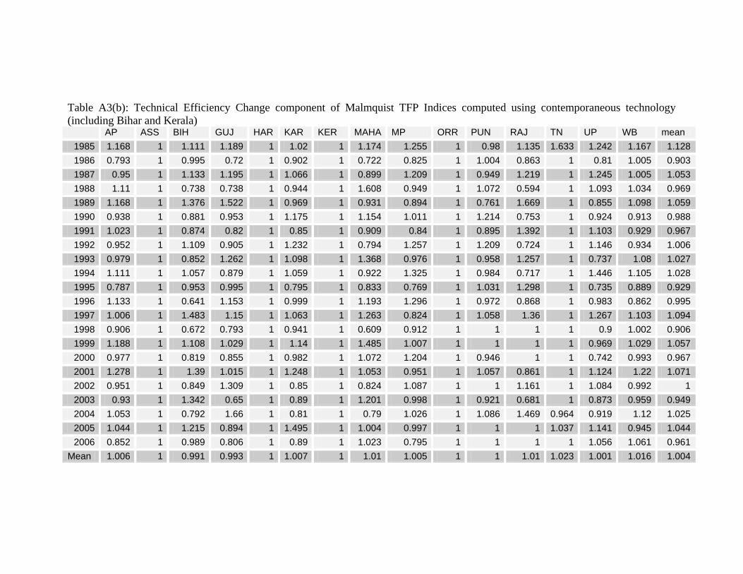
Table A3(b): Technical Efficiency Change component of Malmquist TFP Indices computed using contemporaneous technology (including Bihar and Kerala) AP ASS BIH GUJ HAR KAR KER MAHA MP ORR PUN RAJ TN UP WB mean

1985 1.168 1 1.111 1.189 1 1.02 1 1.174 1.255 1 0.98 1.135 1.633 1.242 1.167 1.128 1986 0.793 1 0.995 0.72 1 0.902 1 0.722 0.825 1 1.004 0.863 1 0.81 1.005 0.903 1987 0.95 1 1.133 1.195 1 1.066 1 0.899 1.209 1 0.949 1.219 1 1.245 1.005 1.053 1988 1.11 1 0.738 0.738 1 0.944 1 1.608 0.949 1 1.072 0.594 1 1.093 1.034 0.969 1989 1.168 1 1.376 1.522 1 0.969 1 0.931 0.894 1 0.761 1.669 1 0.855 1.098 1.059 1990 0.938 1 0.881 0.953 1 1.175 1 1.154 1.011 1 1.214 0.753 1 0.924 0.913 0.988 1991 1.023 1 0.874 0.82 1 0.85 1 0.909 0.84 1 0.895 1.392 1 1.103 0.929 0.967 1992 0.952 1 1.109 0.905 1 1.232 1 0.794 1.257 1 1.209 0.724 1 1.146 0.934 1.006 1993 0.979 1 0.852 1.262 1 1.098 1 1.368 0.976 1 0.958 1.257 1 0.737 1.08 1.027 1994 1.111 1 1.057 0.879 1 1.059 1 0.922 1.325 1 0.984 0.717 1 1.446 1.105 1.028 1995 0.787 1 0.953 0.995 1 0.795 1 0.833 0.769 1 1.031 1.298 1 0.735 0.889 0.929 1996 1.133 1 0.641 1.153 1 0.999 1 1.193 1.296 1 0.972 0.868 1 0.983 0.862 0.995 1997 1.006 1 1.483 1.15 1 1.063 1 1.263 0.824 1 1.058 1.36 1 1.267 1.103 1.094 1998 0.906 1 0.672 0.793 1 0.941 1 0.609 0.912 1 1 1 1 0.9 1.002 0.906 1999 1.188 1 1.108 1.029 1 1.14 1 1.485 1.007 1 1 1 1 0.969 1.029 1.057 2000 0.977 1 0.819 0.855 1 0.982 1 1.072 1.204 1 0.946 1 1 0.742 0.993 0.967 2001 1.278 1 1.39 1.015 1 1.248 1 1.053 0.951 1 1.057 0.861 1 1.124 1.22 1.071 2002 0.951 1 0.849 1.309 1 0.85 1 0.824 1.087 1 1 1.161 1 1.084 0.992 1 2003 0.93 1 1.342 0.65 1 0.89 1 1.201 0.998 1 0.921 0.681 1 0.873 0.959 0.949 2004 1.053 1 0.792 1.66 1 0.81 1 0.79 1.026 1 1.086 1.469 0.964 0.919 1.12 1.025 2005 1.044 1 1.215 0.894 1 1.495 1 1.004 0.997 1 1 1 1.037 1.141 0.945 1.044 2006 0.852 1 0.989 0.806 1 0.89 1 1.023 0.795 1 1 1 1 1.056 1.061 0.961

Mean 1.006 1 0.991 0.993 1 1.007 1 1.01 1.005 1 1 1.01 1.023 1.001 1.016 1.004

Table A3(c): Technical Change component of Malmquist TFP Indices computed using contemporaneous technology (including Bihar and Kerala) AP ASS BIH GUJ HAR KAR KER MAHA MP ORR PUN RAJ TN UP WB mean

1985 0.959 1.034 1.144 0.997 1.081 1.03 1.203 0.837 1.011 0.752 1.099 0.796 0.94 0.954 1.082 0.987 1986 1.151 1.039 1.136 1.127 1.048 1.145 1.054 1.181 1.184 1.157 0.973 1.124 1.097 1.069 1.148 1.107 1987 0.976 0.856 1.078 1.01 1.152 0.948 1.003 0.924 0.925 0.899 1.125 0.988 1.062 1.11 1.001 1 1988 0.965 0.958 0.904 0.971 1.23 0.984 0.972 0.91 0.904 1 1.419 1.032 0.898 1.066 0.913 1 1989 1.009 0.887 1.028 1.024 0.835 0.96 1.086 1.128 0.95 1.143 0.765 1.095 1.124 0.927 0.999 0.991 1990 1.034 1.095 0.954 1.052 1.34 1.01 0.94 1.035 1.04 1.074 1.213 1.051 1.002 1.148 0.983 1.06 1991 1.051 0.844 1.327 1.047 0.854 1.105 1.194 0.883 1.129 0.785 0.952 1.089 1.084 0.921 1.139 1.017 1992 1.035 1.011 0.848 1.028 1.175 0.95 0.944 1.098 0.941 1.166 1.094 0.897 0.979 1.074 0.934 1.007 1993 1.068 1.145 1.087 1.045 1.016 1.015 1.162 0.92 1.045 0.844 1.019 0.979 1.213 1.177 1.02 1.046 1994 0.869 0.781 1.022 0.901 0.911 0.903 1.155 0.968 0.832 0.938 0.942 0.939 0.758 0.708 0.809 0.889 1995 1.205 1.234 1.047 1.145 0.989 1.147 1.157 1.003 1.289 0.837 1.02 1.067 1.338 1.368 1.276 1.132 1996 0.932 0.909 1.189 0.977 0.978 1.07 1.23 1.088 0.889 1.291 1.009 0.949 0.886 0.989 0.926 1.014 1997 0.864 1.093 0.842 0.908 1.043 1.015 1.096 0.85 1.131 0.767 1.166 0.966 0.701 0.763 1.117 0.943 1998 1.134 0.899 1.014 1.036 0.951 0.94 0.911 1.053 0.967 1.072 0.929 1.069 1.243 1.074 0.945 1.012 1999 1.037 0.911 1.034 1.02 0.972 0.962 1.004 0.99 0.945 1.007 1.028 1.077 1.101 1.043 0.921 1.002 2000 1.049 0.89 1.027 1.022 1.336 1.116 1.057 0.903 1.028 0.836 1.292 0.897 1.043 1.229 1.037 1.042 2001 0.856 1.431 0.943 0.828 0.874 0.922 0.77 1.036 1.003 1.085 1.027 0.965 0.777 0.896 0.891 0.942 2002 0.958 0.959 1.018 0.989 1.036 1.019 0.934 1.067 1.043 1.057 1.07 1.409 0.937 0.966 1.07 1.03 2003 0.963 0.952 1.043 1.1 1.079 1.009 0.991 1.034 1.021 1.15 1.085 0.851 0.856 1.26 0.913 1.015 2004 0.873 0.994 0.88 0.933 1.017 0.957 1.012 0.936 0.904 0.781 1.24 1.224 0.871 0.836 1.003 0.957 2005 1.183 1.091 1.073 1.037 1.127 1.041 1.058 1.096 1.034 1.222 1.419 0.926 1.249 1.136 0.999 1.107 2006 1.062 0.998 0.964 0.97 0.958 1.051 1.073 0.882 1.055 0.865 1.217 0.911 1.211 0.84 1.089 1.004

Mean 1.006 0.991 1.022 1.005 1.037 1.011 1.04 0.987 1.007 0.975 1.085 1.006 1.002 1.012 1.005 1.012

Table A4(a): Malmquist TFP Indices computed using contemporaneous technology (excluding Bihar and Kerala) AP ASS GUJ HAR KAR MAHA MP ORR PUN RAJ TN UP WB mean

1985 1.123 1.038 1.186 1.128 0.999 1.232 0.982 0.752 1.076 0.903 1.535 1.184 1.675 1.117 1986 0.913 1.039 0.811 1.061 1.003 0.976 0.853 1.154 0.983 0.969 1.097 0.879 1.131 0.985 1987 0.928 0.856 1.208 1.14 1.021 1.118 0.831 0.9 1.065 1.204 1.062 1.36 1.047 1.047 1988 1.072 0.902 0.718 1.199 0.944 0.859 1.462 1 1.469 0.613 0.899 1.165 0.924 0.988 1989 1.182 0.911 1.541 0.881 0.994 0.85 1.049 1.192 0.596 1.829 1.123 0.796 1.037 1.035 1990 0.972 1.062 1 1.318 1.107 1.051 1.194 1.025 1.454 0.792 1.008 1.048 0.727 1.042 1991 1.048 0.844 0.861 0.863 0.86 0.968 0.805 0.79 0.876 1.515 1.084 1.015 0.886 0.941 1992 0.99 1.01 0.934 1.159 1.159 1.034 0.871 1.156 1.288 0.649 0.99 1.235 0.816 1.007 1993 1.035 1.144 1.311 1.015 1.136 1.028 1.258 0.844 1.001 1.231 1.213 0.866 1.059 1.079 1994 0.965 0.787 0.794 0.911 1.031 1.12 0.9 0.938 0.992 0.675 0.782 1.023 0.919 0.903 1995 0.949 1.234 1.176 0.991 0.973 0.981 0.862 0.843 1.081 1.38 1.338 1.004 1.111 1.059 1996 1.052 0.912 1.055 0.971 1.003 1.131 1.259 1.292 1.001 0.827 0.878 0.973 0.844 1.006 1997 0.881 1.093 1.059 1.047 1.136 0.933 1.074 0.769 1.165 1.308 0.718 0.968 1.189 1.013 1998 1.027 0.912 0.829 0.937 0.931 0.882 0.651 1.073 0.936 1.069 1.243 0.966 0.958 0.945 1999 1.232 0.926 1.05 1.005 1.233 0.981 1.443 1.003 1.055 1.078 1.125 1.011 0.951 1.076 2000 1.025 0.907 0.88 1.337 1.025 1.236 0.957 0.844 1.187 0.897 1.043 0.913 1.028 1.012 2001 1.104 1.431 0.84 0.903 1.13 0.957 1.09 1.084 1.085 0.831 0.79 1.007 1.085 1.014 2002 0.912 0.959 1.294 1.036 0.868 1.129 0.881 1.057 1.062 1.635 0.96 1.047 1.048 1.053 2003 0.895 0.96 0.715 1.079 0.833 1.02 1.24 1.15 1.009 0.579 0.855 1.101 0.88 0.93 2004 0.919 0.997 1.549 1.086 0.874 0.927 0.741 0.784 1.464 1.798 0.84 0.769 1.129 1.026 2005 1.236 1.091 0.927 1.128 1.412 1.032 1.098 1.212 1.449 0.926 1.295 1.296 0.937 1.144 2006 0.914 0.998 0.782 0.965 1.114 0.917 0.904 0.867 1.294 0.911 1.195 0.887 1.167 0.983

Mean 1.012 0.992 0.997 1.046 1.028 1.011 0.997 0.975 1.096 1.016 1.03 1.013 1.01 1.017

Table A4(b): Technical Effciency Change component of Malmquist TFP Indices computed using contemporaneous technology (excluding Bihar and Kerala) Year AP ASS GUJ HAR KAR MAHA MP ORR PUN RAJ TN UP WB mean

1985 1.168 1 1.189 1 0.961 1.226 1.174 1 0.978 1.136 1.633 1.242 1.614 1.161 1986 0.794 1 0.72 1 0.906 0.824 0.723 1 1.005 0.863 1 0.83 1.026 0.892 1987 0.951 1 1.196 1 1.098 1.209 0.899 1 0.961 1.219 1 1.215 1.061 1.057 1988 1.114 1 0.738 1 0.945 0.949 1.607 1 1.059 0.594 1 1.093 0.965 0.982 1989 1.185 1 1.525 1 1.008 0.895 0.931 1 0.776 1.669 1 0.863 1.036 1.044 1990 0.921 1 0.95 1 1.163 1.011 1.154 1 1.225 0.753 1 0.914 0.777 0.981 1991 1.027 1 0.822 1 0.915 0.972 0.916 1 0.886 1.392 1 1.094 0.924 0.988 1992 0.953 1 0.907 1 1.223 1.086 0.789 1 1.187 0.724 1 1.156 0.862 0.981 1993 0.979 1 1.258 1 1.097 0.988 1.372 1 0.979 1.257 1 0.734 1.036 1.042 1994 1.111 1 0.888 1 1.012 1.362 0.925 1 1.021 0.722 1 1.453 1.108 1.031 1995 0.794 1 1.037 1 0.911 0.763 0.854 1 1 1.288 1 0.723 0.886 0.933 1996 1.185 1 1.106 1 1.015 1.269 1.187 1 1 0.889 1 0.98 0.893 1.035 1997 0.947 1 1.136 1 1.081 0.815 1.234 1 1 1.329 1 1.292 1.064 1.06 1998 0.906 1 0.808 1 0.912 0.911 0.631 1 1 1 1 0.899 1.006 0.922 1999 1.188 1 1.007 1 1.136 1.009 1.484 1 1 1 1 0.969 1.032 1.056 2000 0.977 1 0.858 1 0.954 1.201 1.034 1 1 1 1 0.742 0.994 0.976 2001 1.285 1 1.015 1 1.145 0.949 1.053 1 1 0.862 1 1.124 1.224 1.045 2002 0.949 1 1.309 1 0.855 1.087 0.826 1 1 1.161 1 1.084 0.986 1.013 2003 0.928 1 0.65 1 0.805 0.999 1.198 1 0.968 0.681 1 0.873 0.981 0.918 2004 1.051 1 1.66 1 0.898 1.026 0.793 1 1.033 1.469 0.964 0.919 1.093 1.049 2005 1.044 1 0.894 1 1.428 0.997 1 1 1 1 1.037 1.141 0.947 1.031 2006 0.859 1 0.806 1 1.097 0.905 1.023 1 1 1 1 1.056 1.108 0.985

Mean 1.006 1 0.993 1 1.017 1.01 1.01 1 1 1.01 1.023 1.001 1.018 1.007

Table A4(c): Technical Change component of Malmquist TFP Indices computed using contemporaneous technology (excluding Bihar and Kerala) AP ASS GUJ HAR KAR MAHA MP ORR PUN RAJ TN UP WB mean

1985 0.962 1.038 0.998 1.128 1.04 1.005 0.837 0.752 1.1 0.795 0.94 0.953 1.038 0.962 1986 1.151 1.039 1.126 1.061 1.107 1.185 1.181 1.154 0.978 1.124 1.097 1.058 1.102 1.103 1987 0.976 0.856 1.01 1.14 0.93 0.925 0.924 0.9 1.109 0.988 1.062 1.119 0.987 0.991 1988 0.962 0.902 0.974 1.199 0.999 0.905 0.91 1 1.387 1.031 0.899 1.066 0.957 1.007 1989 0.997 0.911 1.01 0.881 0.986 0.95 1.127 1.192 0.769 1.095 1.123 0.922 1.001 0.991 1990 1.055 1.062 1.053 1.318 0.952 1.04 1.035 1.025 1.187 1.052 1.008 1.147 0.936 1.063 1991 1.021 0.844 1.047 0.863 0.941 0.995 0.879 0.79 0.989 1.088 1.084 0.928 0.958 0.952 1992 1.038 1.01 1.03 1.159 0.947 0.953 1.104 1.156 1.085 0.897 0.99 1.069 0.946 1.027 1993 1.057 1.144 1.042 1.015 1.036 1.04 0.917 0.844 1.022 0.979 1.213 1.18 1.022 1.035 1994 0.869 0.787 0.894 0.911 1.019 0.822 0.973 0.938 0.971 0.935 0.782 0.704 0.83 0.875 1995 1.196 1.234 1.134 0.991 1.069 1.285 1.009 0.843 1.081 1.072 1.338 1.388 1.253 1.136 1996 0.888 0.912 0.954 0.971 0.988 0.892 1.061 1.292 1.001 0.93 0.878 0.993 0.945 0.972 1997 0.93 1.093 0.932 1.047 1.05 1.145 0.871 0.769 1.165 0.984 0.718 0.749 1.117 0.955 1998 1.134 0.912 1.027 0.937 1.022 0.967 1.031 1.073 0.936 1.069 1.243 1.074 0.952 1.025 1999 1.037 0.926 1.043 1.005 1.085 0.973 0.972 1.003 1.055 1.078 1.125 1.043 0.921 1.019 2000 1.049 0.907 1.025 1.337 1.075 1.029 0.925 0.844 1.187 0.897 1.043 1.23 1.035 1.036 2001 0.859 1.431 0.828 0.903 0.987 1.008 1.035 1.084 1.085 0.965 0.79 0.896 0.886 0.97 2002 0.961 0.959 0.989 1.036 1.016 1.039 1.066 1.057 1.062 1.409 0.96 0.966 1.062 1.04 2003 0.964 0.96 1.1 1.079 1.035 1.021 1.035 1.15 1.042 0.851 0.855 1.26 0.897 1.013 2004 0.874 0.997 0.933 1.086 0.973 0.904 0.935 0.784 1.418 1.224 0.871 0.836 1.033 0.977 2005 1.183 1.091 1.037 1.128 0.988 1.034 1.098 1.212 1.449 0.926 1.249 1.136 0.99 1.11 2006 1.064 0.998 0.97 0.965 1.016 1.013 0.884 0.867 1.294 0.911 1.195 0.84 1.053 0.998

Mean 1.006 0.992 1.005 1.046 1.011 1.001 0.987 0.975 1.096 1.006 1.007 1.012 0.993 1.01