trends and variation in california's water · pdf filetrends and variation in...
TRANSCRIPT

Trends and Variation in
California’s Water Footprint Julian Fulton & Heather Cooley (Pacific Institute),
Susana Cardenas & Fraser Shilling (UC Davis)
California uses goods and services made in the US and elsewhere, requiring
water and impacting aquatic systems. This is equivalent to California’s Water
Footprint. This Footprint has grown in the last 20 years, beyond what might be
expected from population growth alone. This report describes trends analysis for
the Footprint, as well as estimation of the variation and confidence intervals
around the mean.
December 15, 2013
Topic: Sustainability Trends and Variation in California's Water Footprint
CA Water Plan Update 2013 Vol 4 Reference Guide Page 1
1
Trends and Variation in California’s Water Footprint
Julian Fulton and Heather Cooley
(Pacific Institute)
&
Susana Cardenas and Fraser Shilling
(University of California, Davis)
Report for the California Department of Water Resources and the US
Environmental Protection Agency under agreement # 4600007984, Task Order
No. SIWM-8 to UC Davis and agreement # 201121440-01 to Pacific Institute.
Suggested Citation: Fulton, J., S. Cardenas, H. Cooley, and F. Shilling. 2013. Trends and Variation
in California’s Water Footprint. Report to the California Department of Water Resources and US
Environmental Protection Agency, Pp. 42
About the Authors: Julian Fulton is a Ph.D. candidate in the Energy and Resources Group at
the University of California at Berkeley and a research affiliate with the Pacific Institute Water
Program. Heather Cooley is the Co-Director of the Pacific Institute Water Program. Susana
Cardenas is a graduate student in UC Davis’ Ecology Graduate Group, where she specializes in
measuring ecosystem services and values. Fraser Shilling is a research scientist at UC Davis,
Department of the Environmental Science and Policy and the project lead of the Water
Sustainability Indicators Framework, California Water Plan Update 2013.
Topic: Sustainability Trends and Variation in California's Water Footprint
CA Water Plan Update 2013 Vol 4 Reference Guide Page 2
2
Contents I. Summary and Organization of the Report ............................................................................... 3
II. Evaluating Trends in California’s Water Footprint ................................................................. 3
II.A. Introduction ...................................................................................................................... 3
II.B. Water Footprint Applications ........................................................................................... 6
Water footprint assessment as a tool for the general public .................................................... 6
Water footprint assessment as a tool for corporations ............................................................. 7
Water footprint assessment as a tool for water managers ....................................................... 7
II.C. Analytical Approach ........................................................................................................ 8
II.C. Methods and Data Sources for Calculating Water Footprint Factors ............................ 10
Agricultural Products ............................................................................................................. 12
Industrial Products ................................................................................................................. 13
Energy Products ..................................................................................................................... 13
Trade Data ............................................................................................................................. 15
Regional Analysis .................................................................................................................. 16
II.D. Results and Discussion ................................................................................................... 17
The Water Footprint of Energy Consumption in California .................................................. 17
Trends in California’s Water Footprint ................................................................................. 19
Virtual Water Exports ............................................................................................................ 21
Regional Analysis of California’s Water Footprint ............................................................... 21
II.E. Conclusions .................................................................................................................... 25
III. Measuring Water Footprint Variability ................................................................................. 27
III.A. Introduction .................................................................................................................... 27
III.B. Methods .......................................................................................................................... 27
Data Sources and Transformations: Agricultural Production Variability ............................. 27
Data Sources and Transformations: Income and Diet-Based Variability .............................. 28
Analysis: Agricultural Production ......................................................................................... 28
Analysis: Income and Diet .................................................................................................... 29
III.C. Results ............................................................................................................................ 29
Agricultural Production ......................................................................................................... 29
Effect of Income and Diet ..................................................................................................... 32
III.D. Discussion ...................................................................................................................... 35
IV. Issues, Data Gaps & Recommendations for Future Work..................................................... 36
V. Citations ................................................................................................................................. 39
Topic: Sustainability Trends and Variation in California's Water Footprint
CA Water Plan Update 2013 Vol 4 Reference Guide Page 3

3
I. Summary and Organization of the Report
This report describes two main findings of the Water Footprint (WF) for California: the change
in the total WF and changes in components of the WF over time; and sources of variation in the
WF. California’s WF has increased over the last 20 years, beyond what would be expected from
an increase in population. Twenty years ago, California sustained itself using primarily goods
produced in California. It now gets most its goods from sources outside the state, from sources
within the US and elsewhere. This has resulted in the state’s current WF being primarily located
outside the state. The WF for agricultural goods consumed in California, the vast majority of the
WF, are from a combination of naturally-occurring precipitation and moisture (“Green Water”)
and water applied during irrigation (“Blue Water”). The amount of water applied for specific
crops varies among and within years, resulting in variability around the mean WF of between +
13% (1992) + 9% (2007).
The first section of the report discusses time as a source of variation in total WF, including
evaluation of trends in important components of the WF (e.g., agriculture and energy
production). The second section of the report discusses sources of variability in the WF and how
this variability changes over time. The final section of the report discusses overall conclusions
and remaining questions.
II. Evaluating Trends in California’s Water Footprint
II.A. Introduction
Throughout much of the twentieth century, California’s water use increased as the population
and economy grew. Since the 1970s, however, total water withdrawals for agricultural and
urban purposes in California have remained more or less stable (Figure 1). During this same
period, the state’s population nearly doubled, and the economy quadrupled in constant dollar
terms (CDF 2011; USDC-BEA 2012). These trends suggest that California’s overall water
productivity has improved, both as a function of per capita use and economic output. This
water productivity increase has resulted from the adoption of more efficient practices in nearly
all sectors of society, from households and businesses to farms, factories, and power plants, as
well as reductions in water-intensive manufacturing and growth of the service sector (Gleick et
al. 2005; Rich 2009; Hanak et al. 2012).
Topic: Sustainability Trends and Variation in California's Water Footprint
CA Water Plan Update 2013 Vol 4 Reference Guide Page 4

4
Figure 1. Trends in California’s Population, Freshwater Withdrawals, and state-level GDP
Sources: DWR various1; CDF 2011; USDC 2012
These metrics of increasing productivity, while useful, do not fully capture the total amount of
water required to support California’s growing population and economy and therefore provide
an incomplete picture of California’s overall water use. Many of the goods consumed in
California – and the water required to produce those goods – are imported from locations
outside the state’s borders. Likewise, many of the goods produced in California are exported to
other regions. This movement of goods effectively results in the transfer of the benefits and
burdens of water use into and out of California.
Traditionally water management has been thought of as a local or regional issue, but
globalization has forged increasing interconnectedness among people and economies. As
shown in Figure 2, California has rapidly integrated into the global economy in recent decades.
The value of international imports is now almost three times what it was two decades ago,
while domestic imports (i.e., goods imported into California from other U.S. states) have also
grown substantially in price-adjusted terms (USDC-BC 2010). Exports have also grown, although
1 These data have been collected by DWR staff from older versions of Bulletin 160 (1972-1985), Annual Reports
prepared by District Staff (1989-1995) and the Water Portfolio from California Water Plan Update 2013 (1998-
2010)
-
100
200
300
400
500
600
Ind
ex 1
97
2 =
10
0
California Economy, Population, and Water Use
Real Gross State Product
Population
Freshwater Withdrawals
Topic: Sustainability Trends and Variation in California's Water Footprint
CA Water Plan Update 2013 Vol 4 Reference Guide Page 5

5
to a lesser extent (see Error! Reference source not found.).2 Thus as Californians’ consumption
patterns have become more integrated with the global economy through trade, the water
embedded in those trade flows – also referred to as “virtual water” – plays an increasing role in
California’s overall demand for water and its relationship with water resource conditions
outside the state’s borders.
Figure 2. Trends in California’s International and Domestic Trade
Source: U.S. Department of Commerce, Census Bureau
The “water footprint” has emerged as one tool for quantifying and evaluating the complex ways
in which human activities affect and are affected by the world’s water resources. In 2012, the
Pacific Institute completed the first comprehensive assessment of California’s water footprint
(Fulton et al. 2012). The assessment estimated that California’s total water footprint in 2007
was about 64 million acre-feet, more than double the annual average combined flows of the
state’s two largest rivers, the Sacramento and San Joaquin Rivers. The water footprint of the
average Californian is about 1,500 gallons per day (GPCD), slightly less than the average
American (1,600 GPCD) but considerably more than an average resident in other highly
industrialized countries (1,100 GPCD) (Mekonnen and Hoekstra 2011). Additionally, the study
found that about 70 percent of California’s water footprint is external, meaning that
Californians are highly dependent on water resources from outside the state’s borders. Over
two-thirds of this water is from other U.S. states while less than one-third is from foreign
countries.3
2 Throughout the report the terms export and import are used to imply movement across California’s border to
both international and domestic trading partners. 3 For further discussion and more detailed analysis on the types of products and locations related to California’s
water footprint, see Fulton et al. (2012).
1992 1997 2002 2007 2011
-
100
200
300
400
500
600
700
800
900
Bill
ion
s o
f 2
00
5 d
olla
rs Int'l Import Dom Import
Int'l Export Dom Export
Topic: Sustainability Trends and Variation in California's Water Footprint
CA Water Plan Update 2013 Vol 4 Reference Guide Page 6

6
Potential WF User Groups
Water managers
Agricultural community
Corporations
Environmental groups
Tax/Ratepayer organizations
General public
This report extends our initial assessment in three ways. First, we expanded the scope of
products beyond agricultural, industrial, and direct uses, to include energy products, e.g.,
electricity, natural gas, and transportation fuels. All of these forms of energy require water at
various production stages, from extraction to generation. Second, we evaluated historic trends
in California’s water footprint over the past two decades as a result of changes in production,
trade, and consumption patterns. Lastly, we analyzed the water footprints of California’s ten
hydrologic regions.
II.B. Water Footprint Applications
A water footprint assessment can be conducted at various scales for a variety of purposes. For
example, an individual may conduct a personal water footprint assessment and based on the
results, change his/her consumption patterns, i.e., reduce overall consumption levels and
substitute water-intensive products with less
water-intensive products. Additionally, a
corporation may conduct a water footprint
assessment to examine water risk to its
operations and identify actions to minimize
those risks. In this section, we provide
additional examples of various water footprint
applications.
Water footprint assessment as a tool for the general public
As the general public becomes more aware of resource challenges around the world, there is a
growing interest in characterizing our dependence and impacts on these resources. Over the
past decade, there has been a proliferation of footprint accounting methods, e.g., carbon
footprint, ecological footprint, and water footprint.
As described above, the consumption of goods and services requires the delivery of water
through natural and engineered pathways and return of wastewater to the environment, and
greater levels of consumption typically result in a larger water footprint. There are several
factors that affect an individual’s water footprint. These include:
1) Diet – food consumption is the largest component of an individual’s water footprint and
eating water-intensive produces, such as meat, will increase this water footprint;
2) Income – consumption of goods and services tends to increase with income, as those
that make more money, tend to consume more products and more water-intensive
products and services; and
Topic: Sustainability Trends and Variation in California's Water Footprint
CA Water Plan Update 2013 Vol 4 Reference Guide Page 7

7
3) Supply Chain Length – the further products and services are produced from the
consumer, the greater the water footprint of consumption is likely to be.
Because there is variation in income in California and the US, as there is elsewhere in the world,
it is useful to estimate water footprint using income classes as one way to control for this
variation. The Water Footprint Network has developed an online calculator that estimates the
water footprint based on income.4 The calculator can be used by individuals, or in combination
with Census data to estimate the water footprints of communities.
Water footprint assessment as a tool for corporations
Corporations, as the suppliers of goods and services that individuals consume, play a large role
in determining the water footprint of products they offer. Over the past several years,
corporations have been using water footprint assessments to evaluate their water-related risks
(Morrison et al. 2010, CDP 2010, Hoekstra et al. 2011). A corporate water footprint assessment
includes two major components:
the operational water footprint, i.e. the direct water use by the business in its own
operations, and
the supply-chain water footprint, i.e. the water use in the business’s supply chain.
Typically, the supply-chain water footprint, often ignored in traditional water assessments, is
much larger than the operational water footprint. Among the corporations that have conducted
water footprint assessments include SABMiller, the Coca Cola Company, PepsiCo, Dole Food
Company, Barilla Pasta, and Levi Strauss & Co. (e.g., Coca-Cola and The Nature Conservancy,
2010; SAB Miller and the World Wildlife Fund-UK, 2011; Jeffries et al., 2009).
The different methodologies and their application are still being developed and transparent
case studies are needed that apply the techniques across the entire supply chain, thereby
reflecting the effects of European production and consumption on water scarce river basins
outside Europe.
Water footprint assessment as a tool for water managers
The concept of virtual (or embedded) water can help inform water-management decisions. For
example, coupling virtual water with economic information describing the production value of a
crop can strengthen agricultural water management. For example, Spain was the first country
in the European Union to include a water footprint analysis into its river basin management
plans. The analysis, conducted in 2009, included questions on when and where water footprints
exceed water availability, how much of a catchment's total water footprint is used in producing
4 http://www.waterfootprint.org/?page=cal/waterfootprintcalculator_indv
Topic: Sustainability Trends and Variation in California's Water Footprint
CA Water Plan Update 2013 Vol 4 Reference Guide Page 8

8
exports, and the amount and value of crops produced per unit of water (WFN 2012). Also in
Spain, a 2010 study found that 'high virtual water, low economic value' crops, such as cereals,
are widespread in the region, due in part to a legacy of subsidies in the region. An expansion of
low water consumption and high economic value crops, such as vineyards, was identified as a
potentially important measure for more efficient allocation of water resources (Aldaya et al.
2010). The study concludes that the agricultural sector will need to modify its water use if it is
to achieve significant water savings and environmental sustainability. Pricing is one mechanism
to allocate water to those crops that generate the highest economic value at low water demand
(Bio Intelligence 2012a).
II.C. Analytical Approach
A water footprint assessment provides a metric and methodology for quantifying virtual water.
Because water is constantly circulating and serving multiple uses, the water footprint accounts
only for that portion consumptively used, or “water withdrawn from a source and made
unavailable for reuse in the same basin, such as through conversion to steam, losses to
evaporation, seepage to a saline sink, or contamination (Gleick 2003).” A water footprint is
based on the goods and services consumed and can therefore be calculated at different levels
of consumer activity, i.e., for individuals, households, regions, states, nations, or even all of
humanity.
This analysis uses methods to calculate a water footprint advanced by the Water Footprint
Network, which are described in detail in the Water
Footprint Assessment Manual (Hoekstra et al. 2011). The
basic approach for calculating a water footprint is to
multiply consumptive water use factors (gallons-per-unit of
product) of various products with statistics on the
production, trade, and consumption of those products. It
includes additional quantitative and qualitative features
about the water used, including where the water comes
from and the kinds and quality of water used.
A water footprint has three volumetric components pertaining to consumptive water use:
green water, blue water, and grey water. Green water is the amount of precipitation and soil
moisture that is directly consumed in an activity, such as in growing crops. Blue water is the
amount of surface or groundwater that is applied and consumed in an activity, such as in
growing crops or manufacturing an industrial good. Finally, grey water, is the amount of water
needed to assimilate pollutants from a production process back into water bodies at levels that
Green Water = Rainwater and soil moisture used directly
Blue water = Surface or ground water that is physically applied
Grey Water = Volume of water poluted by runoff and effluent
Topic: Sustainability Trends and Variation in California's Water Footprint
CA Water Plan Update 2013 Vol 4 Reference Guide Page 9
9
meet governing standards, regardless of whether those standards are actually met. 5 The green,
blue and grey water metrics are calculated for individual processes in particular places and then
aggregated based on the consumption patterns of the unit of interest (individual, state, etc.).
The green, blue, and grey water components of a water footprint assessment are often
combined and reported as a single value in the literature. Each, however, has distinct
ecological, social, and economic contexts. Green water pertains to rainwater and soil moisture
occurring where crops are grown and thus may potentially reduce water available for other
land uses, alternative crops, or native vegetation. Blue water, by contrast, represents an
intentional abstraction and allocation of surface or groundwater resources for irrigation,
municipal, and industrial uses, often requiring pumping and conveyance systems to extract and
deliver water. Grey water, as defined in the water footprint literature, is an indicator of water
quality rather than a measure of consumptive water use. Even though the contamination of
surface waters is by definition a consumptive use, contaminated water can often still serve
multiple uses, such as for navigation or cooling. In order to eliminate double counting of
upstream grey water footprints by downstream blue water uses in this analysis, we focus on
California’s blue and green water footprint. Additional analysis is needed on California’s grey
water footprint to depict a more comprehensive water footprint picture of the state.
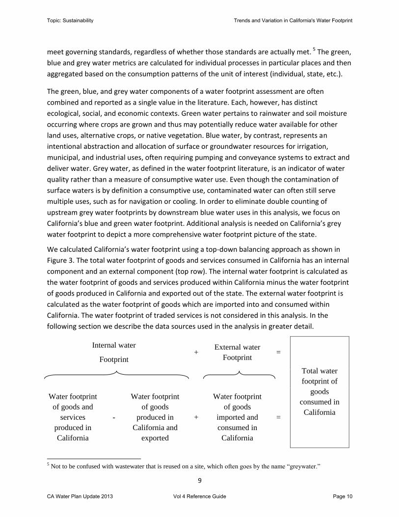
We calculated California’s water footprint using a top-down balancing approach as shown in
Figure 3. The total water footprint of goods and services consumed in California has an internal
component and an external component (top row). The internal water footprint is calculated as
the water footprint of goods and services produced within California minus the water footprint
of goods produced in California and exported out of the state. The external water footprint is
calculated as the water footprint of goods which are imported into and consumed within
California. The water footprint of traded services is not considered in this analysis. In the
following section we describe the data sources used in the analysis in greater detail.
Internal water
Footprint +
External water
Footprint =
Total water
footprint of
goods
consumed in
California
Water footprint
of goods and
services
produced in
California
-
Water footprint
of goods
produced in
California and
exported
+
Water footprint
of goods
imported and
consumed in
California
=
5 Not to be confused with wastewater that is reused on a site, which often goes by the name “greywater.”
Topic: Sustainability Trends and Variation in California's Water Footprint
CA Water Plan Update 2013 Vol 4 Reference Guide Page 10

10
Figure 3: California’s water footprint accounting framework
Source: modified from Hoekstra et al. 2011
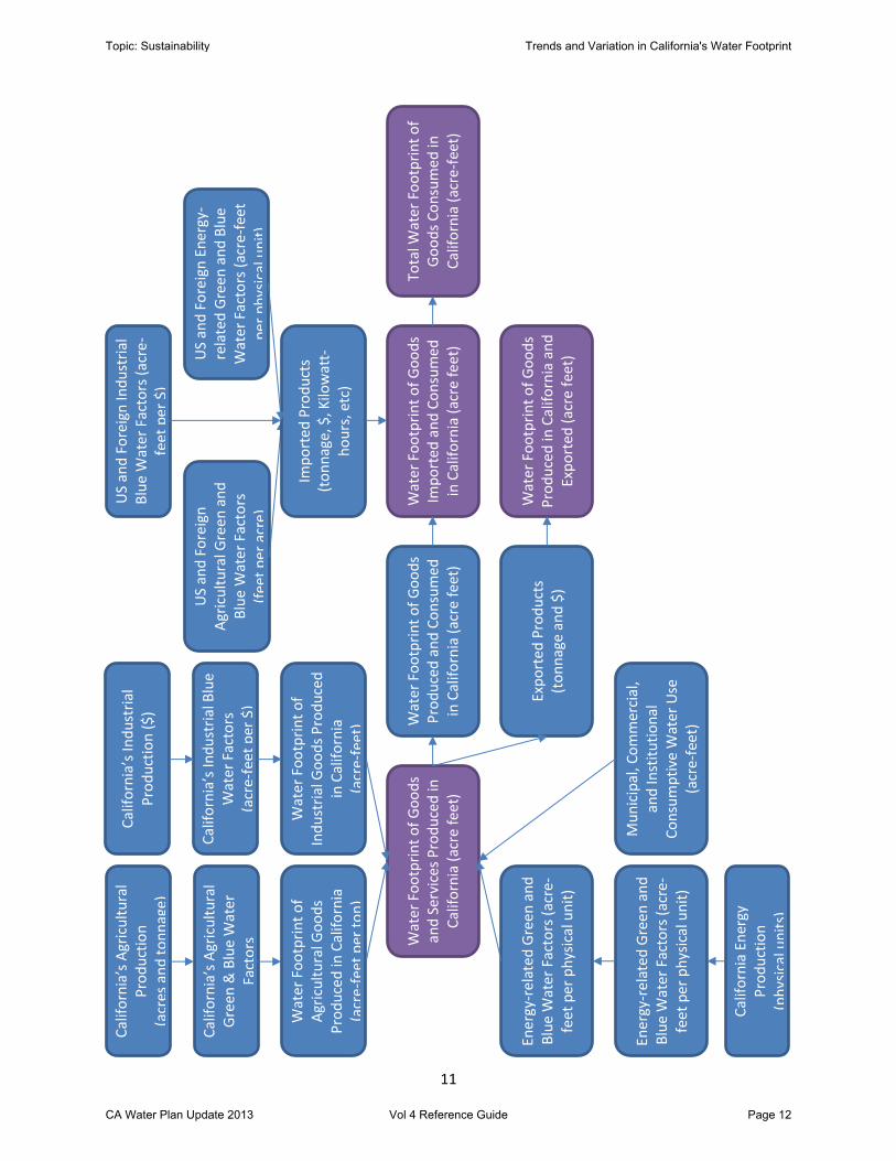
II.C. Methods and Data Sources for Calculating Water Footprint Factors
Figure 4 depicts the modeling framework used to calculate the elements in Figure 3. Each
element of California’s overall water footprint from Figure 3 is shown in a purple box, while the
components used to calculate those elements are in blue boxes. Each line connecting the boxes
depicts a process step in collecting and combining various data sources. The following sections
discuss these data sources and how they were used.
Topic: Sustainability Trends and Variation in California's Water Footprint
CA Water Plan Update 2013 Vol 4 Reference Guide Page 11
11
Cal
ifo
rnia
’s A
gric
ult
ura
l G
reen
& B
lue
Wat
er
Fact
ors
(f
eet
per
acr
e)
Cal
ifo
rnia
’s A
gric
ult
ura
l P
rod
uct
ion
(a
cres
an
d t
on
nag
e)
Wat
er
Foo
tpri
nt
of
Agr
icu
ltu
ral G
oo
ds
Pro
du
ced
in C
alif
orn
ia
(acr
e-f
eet
per
to
n)
Cal
ifo
rnia
’s In
du
stri
al B
lue
Wat
er
Fact
ors
(a
cre
-fee
t p
er $
)
Wat
er
Foo
tpri
nt
of
Ind
ust
rial
Go
od
s P
rod
uce
d
in C
alif
orn
ia
(acr
e-f
eet)
Cal
ifo
rnia
’s In
du
stri
al
Pro
du
ctio
n (
$)
Wat
er
Foo
tpri
nt
of
Go
od
s an
d S
ervi
ces
Pro
du
ced
in
Cal
ifo
rnia
(ac
re f
eet)
Exp
ort
ed P
rod
uct
s (t
on
nag
e an
d $
)
Wat
er
Foo
tpri
nt
of
Go
od
s P
rod
uce
d in
Cal
ifo
rnia
an
d
Exp
ort
ed (
acre
fee
t)
Mu
nic
ipal
, Co
mm
erci
al,
and
Inst
itu
tio
nal
C
on
sum
pti
ve W
ate
r U
se
(acr
e-f
eet)
Tota
l Wat
er F
oo
tpri
nt
of
Go
od
s C
on
sum
ed
in
Cal
ifo
rnia
(ac
re-f
eet)
Wat
er
Foo
tpri
nt
of
Go
od
s Im
po
rted
an
d C
on
sum
ed
in C
alif
orn
ia (
acre
fee
t)
Ener
gy-r
elat
ed
Gre
en
an
d
Blu
e W
ater
Fac
tors
(ac
re-
feet
per
ph
ysic
al u
nit
)
Cal
ifo
rnia
En
ergy
P
rod
uct
ion
(ph
ysic
al u
nit
s)
Ener
gy-r
elat
ed
Gre
en
an
d
Blu
e W
ater
Fac
tors
(ac
re-
feet
per
ph
ysic
al u
nit
)
US
and
Fo
reig
n
Agr
icu
ltu
ral G
ree
n a
nd
B
lue
Wat
er F
acto
rs
(fee
t p
er a
cre)
US
and
Fo
reig
n In
du
stri
al
Blu
e W
ater
Fac
tors
(ac
re-
fee
t p
er $
)
Imp
ort
ed P
rod
uct
s (t
on
nag
e, $
, Kilo
wat
t-h
ou
rs, e
tc)
Wat
er
Foo
tpri
nt
of
Go
od
s P
rod
uce
d a
nd
Co
nsu
med
in
Cal
ifo
rnia
(ac
re f
eet)
US
and
Fo
reig
n E
ner
gy-
rela
ted
Gre
en
an
d B
lue
Wat
er
Fact
ors
(ac
re-f
eet
per
ph
ysic
al u
nit
)
Topic: Sustainability Trends and Variation in California's Water Footprint
CA Water Plan Update 2013 Vol 4 Reference Guide Page 12

12
Figure 4: Modeling framework of water footprint calculation
Agricultural Products
For this analysis, we used California-specific data to estimate the water footprint of goods and
services produced in California.6 Consumptive water use factors for non-energy products were
derived from several California Department of Water Resources (DWR) data sources.
Consumptive use factors for agricultural products were derived from the California Simulation
Evaporation of Applied Water (Cal-SIMETAW) model (Orang et al. 2013), which reconstructs
seasonal crop evapotranspiration (ETc) estimates (in units of acre-feet per acre) for 20 crop
categories from 1992 – 2009 using recorded weather and cropping pattern data. ETc values
were further divided between evapotranspiration of applied water (ETaw) and effective
precipitation (EP).7 ETaw values were used as blue water factors to calculate the blue water
footprint of agricultural products. Green water factors were calculated as EP plus residual soil
moisture (in other words, ETc minus ETaw). These factors were available at the combined
Detailed Analysis Unit-County level (DAU-Co), which could then be aggregated to an individual
county, hydrologic region, and the state as a whole.
Agricultural production statistics were taken from California County Agricultural
Commissioner’s statistics, which provided county-level harvested acreage and production
tonnage for 281 agricultural commodities from 1992 – 2010. Harvested acreage of each
commodity was multiplied by blue and green water factors for the appropriate DWR crop
category to get the total quantity of water required to produce a given crop.8 Water use for a
given crop was then divided by production tonnage for that crop to derive blue and green
water footprint factors in units of acre-feet-per-ton of product. These product-level water
footprint factors were then combined with trade statistics, as described below.
It is important to note that California has non-irrigated agriculture. Specifically, most pasture
and some grains are entirely rainfed. The California County Agricultural Commissioner’s reports
include data on both rainfed and irrigated agriculture. The land use dataset used in Cal-
SIMETAW, however, only provides data on irrigated agriculture. To determine the amount of
land devoted to rainfed crops, we subtracted Cal-SIMETAW irrigated land area statistics for
crop categories from total land area provided in the California County Agricultural
Commissioner’s reports. For rainfed agriculture, we only apply green water factors available
from the Cal-SIMETAW dataset.
6 Note that we used different data sets from Fulton et al. (2012) in order to look in more detail at annual changes
over longer time periods. 7 Cal-SIMETAW yearly values are for a “water year,” which is Oct. 1 – Sept. 30. We assumed that water used for
production in, for example, water year 2007 (Oct. 1, 2006 – Sept. 30, 2007), all pertains to products harvested in
calendar year 2007. 2010 water use values were calculated as the average of 2005-2009. 8 See Appendix 1 in Fulton et al. (2012) for the commodity categories used in this analysis.
Topic: Sustainability Trends and Variation in California's Water Footprint
CA Water Plan Update 2013 Vol 4 Reference Guide Page 13

13
Producing animal products, like meat and dairy, consumes a large amount of water, primarily to
grow the forage and fodder required to feed the animals. Data on the production of animal
products were obtained from the 2007 USDA Census of Agriculture. Using international
biomass-to-product conversion rates published in (Mekonnen and Hoekstra 2010a), we
estimated the amount of feed required to produce these animal products. According to these
sources, an estimated 63.2 million tons of biomass were needed for animal production in
California in 2007. The biomass estimates were multiplied by the water footprints of feed and
forage crops, calculated as described above, to estimate the amount of water required to
produce animal products. The water footprint of animal products, calculated on a gallons-per-
ton basis, for 2007. When trade data were applied, as discussed below, the water footprint
factor was developed for 2007 and applied to all other years analyzed. Other water uses, e.g.,
for washing and hydrating animals and for the processing of animal products, are typically only
around 1% of animal product water footprints (Mekonnen and Hoekstra 2010a) and were not
included in this analysis. The biomass demand from California’s animal product industries
exceeds the supply from in-state sources, thus imported feed crops make a major contribution
to the production of animal products in California.9
Industrial Products
The water footprint associated with industrial products produced in California, as well as direct
residential, commercial, and institutional uses, was derived using Water Portfolios from past
California Water Plan Updates.10 In some cases, only water withdrawals were reported. For
these, we assume that 31% of water withdrawn was consumed.11 For industrial products
produced outside of California, we used national average water footprint factors on a gallons-
per-dollar basis as developed by Mekonnen & Hoekstra (2011). We then combined these
factors with trade data to estimate virtual water flows associated with industrial products into
and out of California.
Energy Products
California’s energy system is complex. The extraction, processing, refining, and generation of
energy products take place within the state’s borders, but there are also significant exchanges
at all of these production stages with neighbors and distant trading partners. To account for
these energy flows, the California Energy Commission’s Public Interest Energy Research
program has sponsored ongoing work at Lawrence Berkeley National Laboratory to create and
9 California exports some animal feed and forage crops, namely alfalfa, and those exports were excluded as an input
to animal products within California. 10
These data have been collected by DWR staff from older versions of Bulletin 160 (1972-1985), Annual Reports
prepared by District Staff (1989-1995) and the Water Portfolio from California Water Plan Update 2013 (1998-
2010). 11
This estimate was based on the average for all urban uses from 1998-2005 as provided by the Technical Guide
from the California Water Plan Update 2009.
Topic: Sustainability Trends and Variation in California's Water Footprint
CA Water Plan Update 2013 Vol 4 Reference Guide Page 14

14
maintain the California Energy Balance (CALEB) database. CALEB manages highly disaggregated
data on energy supply, transformation, and end-use consumption for about 30 different energy
commodities, from 1990 to 2008 (de la Rue du Can et al, 2010). Figure 5 shows an example flow
chart produced by CALEB for 2008, represented in trillion British thermal units of energy (BTUs).
We used CALEB data on the physical units of energy (barrels of oil, million cubic feet of natural
gas, etc.). To identify the origin of imported supplies we used additional information from the
California Energy Commission on electricity (CEC 2013) and from the Energy Information
Administration on natural gas (EIA, 2013a) and oil (EIA, 2013b).
Figure 5: 2008 California Energy Flow Chart (in trillion British thermal units of energy)
Source: de la Rue du Can et al. 2010
Consumptive water use factors for energy were derived from several sources. The National
Renewable Energy Laboratory (NREL) recently completed a review and harmonization of life
cycle factors given by numerous publications on various electricity feedstock and generation
technologies (Meldrum et al. 2013). We used NREL’s median factors for natural gas, coal,
Topic: Sustainability Trends and Variation in California's Water Footprint
CA Water Plan Update 2013 Vol 4 Reference Guide Page 15
15
biomass, and nuclear supplies at the extraction, upgrading, and generation stages, as well as
hydropower. For extraction, processing and refining of oil products we used factors from Wu et
al. (2009). For bioethanol production in the US we used weighted average factors from
Mekonnen and Hoekstra (2010), including refining and on-farm green and blue water
requirements of bioethanol feedstocks. Grey water footprints of energy products were not
calculated as part of this analysis.
Trade Data
As seen in Figure 2, California exports and imports many goods and services. The water
footprint associated with traded goods and services is called a “virtual water flow.” To calculate
these virtual water flows we combined water footprint factors, as described in the previous
section, with trade statistics from the US Department of Transportation’s Freight Analysis
Framework (FAF3) for 1997, 2002, 2007, and 2010 (Southworth et al. 2011). FAF3 combines
Census Bureau and other data into a consistent modeling framework over time, and organizes
data according to the 2-digit level of the Standard Classification of Traded Goods (SCTG) for
both domestic and international trading partners. FAF3 data were not available for 1992. We
therefore used US Department of Transportation’s Commodity Flow Survey (CFS) for 1992
(USDC-BC 1993), which is also organized by SCTG. Because the CFS only includes domestic trade
flows, we assumed that the proportion (by weight) of international to domestic trade flows in
1992 were the same as in 1997.
To calculate the water footprint of products produced in California and exported outside the
state, i.e., “embedded water exports,” trade data were multiplied by blue and green water
footprint factors. For agricultural products, green and blue water footprint factors (gallon per
ton) were aggregated to the 2-digit SCTG level for each trade year and multiplied by export
weights. For industrial products, export values (dollars of sales) for each trade year were
multiplied by the average national industrial blue water footprint factor as provided by
Mekonnen and Hoekstra (2011).
To calculate embedded water imports, trade data were multiplied by blue and green water
footprint factors. For agricultural products, blue and green water footprint factors from
Mekonnen and Hoekstra (2010a, 2010b) were used by taking a weighted average among US
states as well as international trading partners and then aggregated to SCTG categories. For
industrial products, we also used average US and global blue water footprint factors from
Mekonnen and Hoekstra (2011) and multiplied them by the value of imported industrial
products from US and international trading partners. As these datasets are averaged for 1996 –
2005, they were assumed to be the same for each trade year.
Topic: Sustainability Trends and Variation in California's Water Footprint
CA Water Plan Update 2013 Vol 4 Reference Guide Page 16

16
For the analysis of water footprint trends in California, the availability of trade data limited our
analysis to 5-year increments from 1992 to 2007, as well as 2010. For each trade year,
California’s Water Footprint was calculated using the accounting framework shown in Figure 3.
Regional Analysis
We also evaluated regional water footprints related to embedded water flows among
California’s ten hydrologic regions (HRs). While production data were available for these
regions, data were not available for trade and the consumption of products between and within
the regions. Thus, it was not possible to determine whether embedded water stayed within HRs
for local consumption or was transferred for consumption in other parts of the state. Regional
trade or consumption data would allow for a more detailed analysis of regional embedded
water flows within California.
In this analysis, each HR was assessed according to four criteria:
1. Population: the number of people living within each HR.
2. Regional water footprint of goods and services produced in California and
consumed within the HR.
3. Water footprint of goods produced in the HR and consumed in California.
4. Water footprint of goods produced in the HR and exported from California.
To calculate regional water footprints we assumed that California residents consumed the same
quantity and type of products, regardless of where they live, and that the distribution of where
those products were produced was the same for all residents. Fox example, Per-capita green
and blue water footprint estimates were calculated based on California’s internal water
footprint, i.e., excluding the external component, because we were only interested in the
movement of California water within the state. These estimates were multiplied by population
estimates for each HR, which are given in Regional Reports in Volume 2 of the California Water
Plan Update.
To evaluate embedded water flows among regions in California, we used data from Cal-
SIMETAW (Orang et al. 2013) to estimate the amount of blue12 and green water that each of
California’s ten HRs contributes to California’s total water footprint for water year 2007. We
then applied state-level trade data to estimates of blue and green water to distinguish between
embedded water that was exported out of California and that which contributed to
consumption within California.
12
The source of blue water used in production, i.e. groundwater, local surface water or
transferred water, was not distinguished in this analysis.
Topic: Sustainability Trends and Variation in California's Water Footprint
CA Water Plan Update 2013 Vol 4 Reference Guide Page 17
17
II.D. Results and Discussion
The Water Footprint of Energy Consumption in California
We use energy for a variety of purposes, from transporting people and goods around the state,
to powering our homes and businesses. Californians use less energy per person than residents
of 47 other states; however California as a whole is the second most energy-consuming state
due to its large population (EIA, 2012). While large amounts of energy are produced in-state,
California also relies heavily on external sources of electricity, natural gas, and oil.
Here, we provide an assessment of California’s Water Footprint associated with the
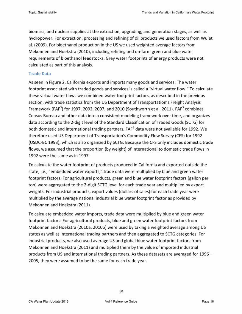
consumption of energy products within the state (herein “Energy Water Footprint”). Figure 6
shows the amount of water required to produce the energy consumed in California between
1990 and 2008. As can be seen, prior to 2003, California’s Energy Water Footprint was about
1.5 MAF. During this period, Methyl Tertiary Butyl Ether (MTBE) was added as an oxygenate to
automotive gasoline to boost octane and reduce air pollution, especially ground-level ozone
and smog. By the end of 2002, however, MTBE was detected in groundwater aquifers across
California and subsequently banned in the state. MTBE was replaced with ethanol starting in
2003. This change, as shown in Figure 6, led to a four-fold increase in California’s Energy Water
Footprint. In 2008, the most recent year in our analysis, the total Energy Water Footprint was
5.6 million acre feet (MAF). Over two-thirds of this amount (4.0 MAF) was green water and the
remainder (1.6 MAF) was blue water. The green water component of California’s Energy Water
Footprint is entirely attributable to bioethanol, most of which is blended with gasoline. The
blue water requirements of bioethanol add a smaller, yet still significant, amount to California’s
Energy Water Footprint (0.4 MAF).
Topic: Sustainability Trends and Variation in California's Water Footprint
CA Water Plan Update 2013 Vol 4 Reference Guide Page 18
18
Figure 6: California’s energy-related green and blue water footprint, 1990-2008
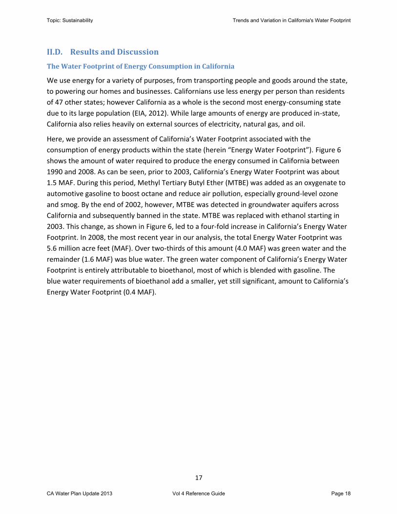
This process of increased blending of bioethanol in California’s gasoline has also accelerated an
externalization of the state’s Energy Water Footprint. Figure 7 shows that from 1990 to 2002
about half of California’s Energy Water Footprint was external. Today, nearly 90% is external.
The import of bioethanol from the U.S. Midwest is the primary driver of this phenomenon,
although increased imports of other fuels, such as oil and natural gas, has also played a minor
role.
Figure 7: California’s energy-related internal and external water footprint, 1990 – 2008
-
1
2
3
4
5
6
7M
illio
n A
cre
Feet
per
Yea
r
Green WF of Ethanol
Blue WF of Ethanol
Blue WF of Oil and Products
Blue WF of Natural Gas (direct consumption)
Blue WF of Electricity Generation
-
1
2
3
4
5
6
7
Mill
ion
Acr
e Fe
et p
er Y
ear
External Energy WF - Foreign
External Energy WF - USA
Internal Energy WF
Topic: Sustainability Trends and Variation in California's Water Footprint
CA Water Plan Update 2013 Vol 4 Reference Guide Page 19

19
California’s Energy Water Footprint has major implications for understanding sustainable
resource management in the context of the water-energy nexus. California’s energy system is
complex, and changes in the system can have an implication for water resources. Our analysis
shows that substituting MTBE with bioethanol increases California’s water footprint. Producing
bioethanol feedstock (e.g., corn) in California has not proven to be economically viable, and as a
result, the water requirements for gasoline additives have come from outside the state’s
borders, primarily from the U.S. Midwest. Summer droughts of 2012, and the subsequent
reductions in ethanol production, highlighted the risk involved in an energy system that derives
inputs from vulnerable areas (EIA, 2012). Perhaps ironically, the legislation that mandated
MTBE substitution with bioethanol was motivated by the human health risks that MTBE
contamination poses to groundwater, thereby shifting a water quality impact that ultimately
affects the availability of water resources to a direct water quantity impact. This suggests that
energy policies designed to minimize risk, whether from power plant air pollution or
groundwater contamination by MTBE, must also take into consideration the impacts to other
resource systems, especially water. Similarly, expanding in-state energy extraction and
generation may also have its downsides. Unconventional fossil fuel extraction, such as shale gas
and oil shale, poses risks to water resources that would become localized if in-state
intensification is pursued. Ultimately there may be more relative tradeoffs than absolute
solutions in California’s Energy-Water Nexus. Nevertheless, the Energy Water Footprint is a
useful tool for integrating decision making for the sustainability of multiple resources.
Trends in California’s Water Footprint
California’s total Water Footprint has changed over time in response to population and
economic growth (Figure 8). Three observations can be drawn from this trend. First, the overall
Water Footprint has increased over time at a rate (4% per year) that exceeds population growth
(1.4% per year). As a result, the Water Footprint of the average Californian has grown from
1,600 gallons per capita daily (GPCD) in 1992 to about 2,300 GPCD in 2010, suggesting that
Californians are consuming more water-intensive products and/or more products than in the
past. It appears California’s water footprint is more tightly correlated with economic growth,
which has proceeded at an average rate of 5.2% per year in real terms, than population growth.
In general these findings suggest that population growth, coupled with economic growth, can
increase demand for water resources unless efficiency gains are made across the supply chain
of products that the population and related economic activities consumes.
Topic: Sustainability Trends and Variation in California's Water Footprint
CA Water Plan Update 2013 Vol 4 Reference Guide Page 20

20
Figure 8: Trend of California’s green and blue water footprint, by internal and external
components, 1992 - 2010
Second, California’s Water Footprint has become increasingly dependent on green water, from
51% in 1992 to 72% in 2010. The growing contribution of green water to California’s Water
Footprint raises concerns about the risk of relying on precipitation and the potential impacts of
climate change. For example, recent droughts in the U.S. Midwest have affected grain supplies
in California and provided evidence of California’s susceptibility to global climatic changes in
regions outside of its borders (EIA 2012). Incidentally, increased dependence on blue water
could also expose California to potentials impacts of climate change since, ultimately, sources
of blue water such as surface water reservoirs and groundwater aquifers, and rivers, canals, and
streams are also directly dependent on the overall precipitation in an area. Nevertheless,
management of blue water offers some flexibility to cope with year-to-year variations in
precipitation.
Third, and perhaps most dramatically, California’s Water Footprint has become increasingly
externalized, from 38% in 1992 to 76% in 2010, meaning that we now rely far more on water
resources from outside of our borders to support our consumption patterns than we did in the
early 1990s. Most of this water is from other parts of the United States, but the percentage of
virtual water from outside of the United States has nearly doubled from 21% to 41% over this
time period. The further externalization of California’s Water Footprint raises concerns about
our ability to manage water resource impacts and risks associated with our demand for goods
and services.
The values calculated in this trends analysis are higher than our initial calculations (Fulton et al,
2012) for three primary reasons. First, we included California’s energy water footprint,
accounting for an additional 5.5 MAF in 2007. Second, consumptive use factors were higher in
Blue
Green
-
20
40
60
80
100
120
1992 1997 2002 2007 2010
Mil
lion A
cre
Fee
t
External
Water
Footprint
Internal
Water
Footprint
Topic: Sustainability Trends and Variation in California's Water Footprint
CA Water Plan Update 2013 Vol 4 Reference Guide Page 21

21
Cal-SIMETAW than in the previously-used model (DWR’s Land and Water Use Survey) due to its
modification of crop water requirement and soil moisture contribution parameters. Finally, the
FAF3 database included modeled values for traded goods that were omitted in the previously-
used database (Commodity Flow Survey) for confidentiality reasons in some industries.
Virtual Water Exports
The water embedded in California’s exports is not captured in its Water Footprint. However, it
has important implications for statewide water management. As shown in Figure 9, more of
California’s water resources are being used to produce goods that are exported and consumed
outside the state’s borders (Figure 9). In 1992, 12 MAF was used to produce goods consumed
outside of California. By 2010, that number had increased to 26 MAF. The value generated by
exports has declined on a per-unit of water basis. In 1992, total exports produced $0.11 per
gallon in revenue for the state whereas by 2007 exports were producing $0.07 per gallon.
Figure 9: Trend in green and blue water embedded in California’s exports, 1992 – 2010
Regional Analysis of California’s Water Footprint
Other sections of the California Water Plan Update describe how water is physically moved and
distributed around the state. There are also, however, transfers of embedded water from
where water is put into production to the location where the product is ultimately consumed.
This section provides a regional assessment of how California’s internal water footprint in 2007
was distributed among the state’s ten Hydrologic Regions (HRs) (10).
Green
Blue
-
5
10
15
20
25
30
1992 1997 2002 2007 2010
Mil
lion A
cre
Fee
t per
Yea
r
Topic: Sustainability Trends and Variation in California's Water Footprint
CA Water Plan Update 2013 Vol 4 Reference Guide Page 22

22
In this analysis, each HR was assessed
according to four criteria:
1. Population: the number of people
living within the HR.
2. Regional water footprint of goods
and services produced in California
and consumed within the HR.
3. Water footprint of goods produced
in the HR and consumed in
California.
4. Water footprint of goods produced
in the HR and exported out of
California.
Results based on these criteria are
discussed below and shown for each HR in
Figures 11Error! Reference source not
found. to 14.
Figure 11 compares California’s HRs by
population. Over half of the population
(19 million people) lives in the South Coast HR. The San Francisco Bay HR is the second most
populated HR, with 6.2 million people. Because we assume that all Californians have the same
per capita water footprint and the same ratio of blue to green water, the most populous HRs
have the largest water footprints (Figure 12). Together, the South Coast and San Francisco Bay
HRs account for 70% of California’s population and thus water footprint.
Figure 10: California’s ten hydrologic
regions
Topic: Sustainability Trends and Variation in California's Water Footprint
CA Water Plan Update 2013 Vol 4 Reference Guide Page 23

23
Figure 11: Population of California’s 10 hydrologic regions
Figure 12: Green and blue water footprints related to goods produced and consumed in
California, by hydrologic region
The next dimension compares the water footprint of goods produced in each HR and consumed
in California (Figure 13). Each HR uses a different amount of green and blue water in
production. Together, this is the volume of water in each HR that is used in the production of
goods and services that are ultimately consumed in California. By this measure, the South Coast
and San Francisco Bay HRs contributes less than 1 MAF to the state’s overall water footprint.
These regions are highly urbanized and have little productive farmland, so overall water use is
lower than in other HRs. By contrast, the three HRs of the Central Valley - Sacramento River,
- 5 10 15 20 25
01-North Coast
02-San Francisco Bay
03-Central Coast
04-South Coast
05-Sacramento River
06-San Joaquin River
07-Tulare Lake
08-North Lahontan
09-South Lahontan
10-Colorado River
Millions
- 2 4 6 8 10
01-North Coast
02-San Francisco Bay
03-Central Coast
04-South Coast
05-Sacramento River
06-San Joaquin River
07-Tulare Lake
08-North Lahontan
09-South Lahontan
10-Colorado River
Million Acre Feet
Topic: Sustainability Trends and Variation in California's Water Footprint
CA Water Plan Update 2013 Vol 4 Reference Guide Page 24

24
San Joaquin River, and Tulare Lake - contribute 70% of the state’s internal water footprint. The
largest contribution of green water to in-state consumption comes from the Sacramento River
region at 1.6 MAF, followed by the North Coast (1.1 MAF). For blue water supply, Tulare Lake
provides the most (5.7 MAF), followed by San Joaquin River (3.6 MAF) and Sacramento River
(3.3 MAF), and to a lesser extent the Colorado River HR (1.5 MAF).
Figure 13: Green and blue water footprints contribution to California’s water footprint, by
hydrologic region
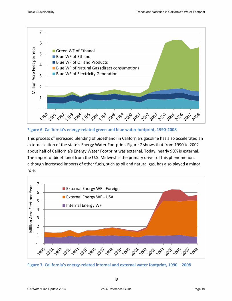
The final dimensions considered, blue and green virtual water export, is water that has been
consumptively used within the HR for the production of exported products. These quantities do
not count towards California’s water footprint but are nevertheless illustrative of whether
water is used in different HRs for in-state consumption or for export. Figure 14 shows that
green virtual water exports originate mostly from the Sacramento River (1.3 MAF), followed by
Tulare Lake (0.7 MAF) and San Joaquin River (0.6 MAF). Greater differences exist for virtual blue
water export, which is highest from Tulare Lake (4.5 MAF), followed by San Joaquin River (2.8
MAF), and Sacramento River (2.7 MAF).
- 2 4 6
01-North Coast
02-San Francisco Bay
03-Central Coast
04-South Coast
05-Sacramento River
06-San Joaquin River
07-Tulare Lake
08-North Lahontan
09-South Lahontan
10-Colorado River
Million Acre Feet
Topic: Sustainability Trends and Variation in California's Water Footprint
CA Water Plan Update 2013 Vol 4 Reference Guide Page 25
25
Figure 14: Green and blue virtual water export out of state from California’s hydrologic
regions
To a large extent, the movement of embedded water within the state reflect the geographic
distribution of Californa’s population, water resources, and productive agricultural land. Much
of the state’s population is concentrated in arid areas. Nevertheless mapping these features can
help planning and decision making in several ways. For example, exchanging embedded water
can be an alternative to transfering bulk water when other conditions for production are
favorable, e.g., availability of arable land. Furthermore, the interconnection of water resources
provides further motivation for regional coordination to address California’s water challenges,
especially engaging with residents and planners in those areas with large water footprints.
Additional data collection and modeling work could support greater insight into interregional
flows of both direct and embedded water within California. For example, using proprietary
input-output databases from IMPLAN could provide additional resolution on how products are
produced and traded within California. Ongoing efforts in other resource arenas, such as energy
and carbon, could also provide synergy for embedded water work. One example is the PECAS
(Production, Exchange, Consumption, Allocation System) model administered by the Institute of
Transportation Studies at UC Davis which is now being supported by the California Energy
Commission’s Public Interest Energy Research program to provide analysis on interregional
energy flows.
II.E. Conclusions
California’s economy consistently ranks among the ten largest in the world and is closely linked
with interstate and global commerce. Much of our economic prosperity is derived from
- 1 2 3 4 5
01-North Coast
02-San Francisco Bay
03-Central Coast
04-South Coast
05-Sacramento River
06-San Joaquin River
07-Tulare Lake
08-North Lahontan
09-South Lahontan
10-Colorado River
Million Acre Feet
Topic: Sustainability Trends and Variation in California's Water Footprint
CA Water Plan Update 2013 Vol 4 Reference Guide Page 26

26
exporting goods and services and, likewise, many imports are integral to our high living
standards. In terms of water, this means that our “water footprint” falls not only on water
resources from within the state’s borders, but also on water resources in locations where goods
that we consume are produced. A water footprint analysis is useful in understanding the
complex interconnections between local water resource management and water use impacts
and risks related to California’s place in the global economy.
Our 2012 report - California’s Water Footprint - was the first of its kind, both for its fresh
perspective on water use in California and for its novelty in carrying out an assessment at the
sub-national level. Several insights emerged from this study. For example, we found that 70% of
California’s water footprint is associated with goods produced outside of its border, indicating
that California is net importer of virtual water. The reverse is true for the U.S. as a whole, where
70% of the nation’s water footprint is associated with goods produced inside its borders. Such a
contrast highlights the importance of carrying out water footprint assessments at different
scales as well as the relevance of findings to policy and management institutions at difference
levels of government.
A second round of analysis was supported by California’s Department of Water Resources and
extended our initial assessment in three dimensions. First, we expanded the scope of products
beyond agricultural, industrial, and direct use, to include energy products like electricity,
natural gas, and transportation fuels. Water use in California’s energy system was found to be
most intensive for transportation fuels, especially since the state mandated the use of ethanol
as an oxygenate in gasoline in 2004. Second, we have identified trends in the evolution of
California’s water footprint over the past two decades, finding that California’s water footprint
has grown by approximately 60% since 1992, while the population has grown by 25% and gross
state product has doubled in real terms. Third, we have analyzed how water embedded in
products is transferred within California’s ten hydrologic regions. The distribution of physical
water through canals and other infrastructure is a key feature of California’s water
management, and the movement of “virtual water” adds a new dimension that can aid water-
related decision making.
Our findings raise several corresponding concerns with respect to sustainability. First,
population growth can increase demand for water resources unless efficiency gains are made
across the supply chain of products that the population consumes. The observation that
California’s Water Footprint is growing at a faster rate than population indicates that
Californians are consuming either more water-intensive products and/or more products.
Second, the proportional contribution of green water to California’s water footprint raises
concerns about the risk of relying on precipitation and the potential impacts of climate change.
Recent droughts in the American Midwest have affected grain supplies in California and
provided evidence of -susceptibility to global climatic changes outside of the state’s borders.
Topic: Sustainability Trends and Variation in California's Water Footprint
CA Water Plan Update 2013 Vol 4 Reference Guide Page 27
27
Third, the externalization of California’s Water Footprint raises concerns about our ability to
manage the water resources related to our footprint. California’s water resources are
increasingly being devoted to exports, while our consumption becomes increasingly reliant on
embedded water in imports (see “External Water Footprint” above). This poses additional
challenges for managing our interaction with water sustainably by considering the risks and
potential impacts to water systems outside of our borders.
III. Measuring Water Footprint Variability
III.A. Introduction
Water Footprint estimates can vary depending on the variability associated with the specific
components in their calculation. Sources of variation include: 1) natural variation in the water
cycle, including rainfall and water available to dilute pollution; 2) variation due to crop types
and irrigation regimes, 3) variation in actual evapotranspiration rates relative to assumed rates,
3) inter-regional differences in water use for a particular product, 4) inter-annual variation in
the consumption of goods and services, 5) variation in water-impacting consumption behavior
(e.g., dietary choices), and 6) variation in consumption rates based on individual income and
other social or economic factors.
Agricultural/food production is the largest component of the water footprint, representing 93%
of the WF in 2007 (Fulton et al. 2012). Considering the importance of agricultural water
demand in California, this section includes an estimate of the impact of the variability in the
water footprint of agriculture production on the total water footprint of the state. This section
also examines how income and dietary choices affect an individual’s water footprint.
III.B. Methods
Data Sources and Transformations: Agricultural Production Variability
Blue water footprint and green water footprint of agricultural production come respectively
from estimates of the total volume of evapotranspiration of applied water in agricultural crops
(ETaw) and the total volume of effective precipitation (EP) multiplied by the irrigated
agricultural area. ETaw and EP estimates by year were obtained from the Cal-SIMETAW model
(Orang et al. 2013). This model was developed by the California Department of Water
Resources and the University of California, Davis to perform daily soil water balance and
determine crop evapotranspiration (ETc), evapotranspiration of applied water (ETaw), and
applied water (AW) for use in California water resources planning.
The Cal-SIMETAW provides seasonal water balance estimates at two geographical scales within
Topic: Sustainability Trends and Variation in California's Water Footprint
CA Water Plan Update 2013 Vol 4 Reference Guide Page 28
28
California: detailed analysis unit (DAU) and county. The ETaw and EP values for the smallest
scale unit of the model (DAU) were used in the analysis. The DAU scale was used in order to
have a range of ETaw and EP values for each crop type. The database provides ETaw and EP
estimates in volume units and as factors, the latter being the estimate of the volume over the
irrigated crop area (ICA) by scale unit. Factors were used in the analysis of variability. In order
to account for scale, values of the DAU distribution are scaled up to the state level, each DAU
factor was weighted by the ICA for that DAU for the corresponding crop and divided by total
ICA for that crop in each year. Once each DAU weighted factor was summed up by crop by year,
weighted ETaw and EP factors were then consistent with the statewide factors used in the
overall water footprint analysis done at the state level.
Data for the other elements of the total water footprint estimate, including the water footprint
of international trade and internal consumption, were from Fulton et al. (2012).
Data Sources and Transformations: Income and Diet-Based Variability
The income tables for specific California counties (Orange, San Bernardino, Los Angeles, and
Riverside) were downloaded from the “Fact Finder” tool on the Census Bureau website. These
tables included proportion of population in each major household-income category (e.g.,
$50,000 to $74,999 per year), as well as basic statistics about household composition and total
number of households.
Data Sources:
Census 2011, American community Survey 2011 estimates of income by county
(http://factfinder2.census.gov/faces/tableservices/jsf/pages/productview.xhtml?pid=ACS_11_1
YR_S1902&prodType=table)
Water Footprint Network, Quick Water Footprint Calculator
(http://www.waterfootprint.org/?page=cal/waterfootprintcalculator_indv)
Water demand delivery data from Santa Ana Watershed Project Authority
(http://www.sawpa.org) Analysis: Agricultural Production
Nine crops were selected for assessing the impact of agricultural water footprint variability on
total water footprint. These crops are: grain, alfalfa, cotton, pasture, vine, other truck crops
(vegetables besides the ones listed in other categories), almond and pistachios, corn, and rice.
The crops selected represent the most water demanding crops grown in California, due to the
extent of their irrigated crop area and higher ETaw and/or EP factors. For this analysis, we
assessed the variability associated with the blue water footprint, i.e., ETaw factors. The same
procedure can be replicated for the green water footprint calculation using EP values.
The variability of ETaw factors around their mean was determined. The range of ETaw factors at
Topic: Sustainability Trends and Variation in California's Water Footprint
CA Water Plan Update 2013 Vol 4 Reference Guide Page 29
29
the DAU level per crop per year were used to define the 95% confidence interval. Using the
upper and lower bounds of the 95% confidence interval of each distribution per crop, we
calculated the percent difference of the 5th percentile and 95th percentile relative to the mean
and applied these estimates to the statewide ETAw and EP factors. The change in the blue
water footprint for each specific crop by year was calculated by multiplying these factors by the
ICA of each specific selected crop (Table 2). The values obtained were included in the
calculation of the blue water footprint for agricultural production, while holding constant the
values for the other crops.
Finally, the variability of the total water footprint for the state was obtained. Once the two
upper and lower values of blue water footprint of agricultural production were obtained
following the steps above, they were applied to the total water footprint. The percentage
variation of these values compared to the original water footprint value indicates the impact of
the agricultural water footprint variability on total water footprint for the state.
Analysis: Income and Diet
The median value in each category was calculated and used to estimate the water footprint.
The Quick Water Footprint Calculator was used to calculate water footprint based on gender,
diet, and income. Three diet choices were provided: vegetarian, average meat consumption,
and high-end meat consumption. For most calculations, “average meat consumption” was
chosen to represent the largest number of people. Because most households have two adults
of opposite gender, the average of male and female water footprint was used and household
income was assumed to represent two adults for the purposes of the water footprint
calculation.
III.C. Results
Agricultural Production
The impact of the variability of the blue water requirements of the nine agricultural crops
selected was assessed based on three components of California’s water footprint (Table 1). The
water footprint of agricultural production varies between -26% and +34% around the mean,
and keeps constant throughout the four years evaluated. The corresponding estimated
variation of California’s blue water footprint does not differ greatly from the water footprint of
agricultural production (-24% to +29% variability), because agricultural production represents ~
80% of the blue water footprint of the state. The variability of water demand from the main
crops evaluated resulted in a variation of -12% to +14% for California’s total water footprint.
This variation has been decreasing over time. For example, in 1992, variation of the total WF
varied between -12% and +14% around the mean and in 2007 variation was -8% to +10%
around the mean. Possible explanations could be the application of better technologies to
Topic: Sustainability Trends and Variation in California's Water Footprint
CA Water Plan Update 2013 Vol 4 Reference Guide Page 30

30
reduce the water demand by crops across the state and higher demand on other components
of the water footprint. One important caveat to consider is that the estimates of variation are
dependent on the model from which the ETaw factors were obtained and its assumptions.
Table 1. Variability in California Water Footprint and its components due to variability of water footprints of the nine main crops statewide
1992 1997 2002 2007
% Variability in CA Water Footprint of Agricultural Production
Lower bound* -27 -27 -27 -26
Upper bound* +33 +33 +34 +33
% Change in CA Blue Water Footprint
Lower bound* -24 -24 -20 -23
Upper bound* +29 +29 +25 +29
% Change in CA Water Footprint
Lower bound* -12 -10 -7 -8
Upper bound* +14 +12 +9 +10
Note: * Lower and upper bounds of the 95% confidence interval.
Note: The average percentage change of the ETaw factors of the upper and lower bounds of
the 95% confidence interval, of all nine crops for the four years included in the analysis, was
37%.
Topic: Sustainability Trends and Variation in California's Water Footprint
CA Water Plan Update 2013 Vol 4 Reference Guide Page 31

31
Table 2. Variability of ETAW factors and blue water footprint (acre-feet) around the state
mean per crop for years 1992, 1997, 2002, 2007.
ETAW factors per crop per year Blue WF per crop per year (feet-
acre)
-95th State mean
+95th ICA -95th State mean +95th
Grain 1992 0.8749 1.2645 1.6541 895,760 783,710 1,132,691 1,481,672
1997 1.0556 1.6023 2.1489 902,580 952,808 1,446,181 1,939,554
2002 0.9614 1.4279 1.8945 655,620 630,298 936,180 1,242,062
2007 0.9274 1.3825 1.8375 533,928 495,185 738,139 981,094
Rice 1992 3.0200 3.1366 5.9400 419,800 1,267,796 1,316,731 2,493,612
1997 3.0400 3.0599 6.1300 552,700 1,680,208 1,691,233 3,388,051
2002 3.1900 3.0406 6.1700 556,300 1,774,597 1,691,500 3,432,371
2007 2.9500 3.0927 6.1200 583,020 1,719,909 1,803,097 3,568,082
Cotton 1992 1.7546 3.0650 4.3753 1,192,720 2,092,797 3,655,667 5,218,537
1997 1.5900 3.0372 4.4844 1,072,435 1,705,203 3,257,234 4,809,265
2002 1.5812 3.1787 4.7761 671,180 1,061,290 2,133,468 3,205,647
2007 1.5946 3.1256 4.6566 456,506 727,940 1,426,850 2,125,761
Corn 1992 1.3880 2.2389 3.0898 398,800 553,535 892,869 1,232,204
1997 1.3387 2.1318 2.9248 641,580 858,915 1,367,689 1,876,463
2002 1.4131 2.3137 3.2143 629,020 888,871 1,455,357 2,021,844
2007 1.3988 2.2719 3.1449 771,467 1,079,123 1,752,669 2,426,216
Alfalfa 1992 2.2076 4.2650 6.3224 1,067,430 2,356,471 4,552,606 6,748,741
1997 2.3125 4.3018 6.2911 1,033,277 2,389,503 4,444,982 6,500,461
2002 2.3279 4.3095 6.2912 1,194,700 2,781,136 5,148,608 7,516,081
2007 2.5554 4.3111 6.0667 1,072,726 2,741,288 4,624,601 6,507,915
Pasture 1992 2.7072 3.5620 4.4168 929,321 2,515,855 3,310,223 4,104,591
1997 2.5514 3.4937 4.4361 867,660 2,213,719 3,031,379 3,849,038
2002 2.4252 3.6141 4.8031 834,160 2,022,974 3,014,776 4,006,577
2007 2.3726 3.6770 4.9815 766,372 1,818,302 2,817,987 3,817,672
Other Truck
1992 1.0123 1.6842 2.3562 742,426 751,534 1,250,430 1,749,326
1997 0.9884 1.7508 2.5132 731,803 723,338 1,281,252 1,839,166
2002 0.9777 1.7072 2.4367 855,890 836,829 1,461,186 2,085,542
2007 0.9580 1.7235 2.4891 874,001 837,257 1,506,345 2,175,432
Almond/ Pistachio
1992 3.0194 4.4814 5.9434 501,870 1,515,350 2,249,083 2,982,815
1997 3.0368 4.5857 6.1347 582,220 1,768,093 2,669,911 3,571,730
2002 3.1915 4.6823 6.1732 726,130 2,317,435 3,399,979 4,482,523
2007 2.9512 4.5372 6.1233 955,339 2,819,353 4,334,588 5,849,824
Vine 1992 1.7582 3.1290 4.4999 728,760 1,281,283 2,280,306 3,279,328
1997 1.7527 2.9913 4.2299 809,495 1,418,797 2,421,446 3,424,094
2002 1.7079 2.8602 4.0125 913,600 1,560,383 2,613,091 3,665,799
2007 1.7973 2.8768 3.9563 871,013 1,565,499 2,505,743 3,445,987
Note: ICA = “Irrigated Crop Area” (acres) in California
Topic: Sustainability Trends and Variation in California's Water Footprint
CA Water Plan Update 2013 Vol 4 Reference Guide Page 32

32
Effect of Income and Diet
Median and mean household incomes in each county were the following: San Bernardino
($51,247 & $65,472), Riverside ($52,883 & $69,898), and Orange ($72,293 & $96,627). There
was considerable variation round these central tendency values, with 4.5% to 6.9% of
households occupying the lowest income category (<$10,000) and 2.9% to 9.4% of households
occupying the highest category (>$200,000).
Relationship between Water Footprint and Income
Beyond a base level of consumption of goods and services, estimated water footprint per capita
increases linearly with income (figure 16). Diet affected both baseline water footprint and rate
of change in footprint with income. Vegetarian diet had the smallest water footprint and high-
end meat consumption the largest. This is because of the investment of virtual water in grains
used to grow animals for consumption, compared to the direct consumption of plant material.
Figure 16. Rate of change in estimated water footprint (m3/capita-year) with individual
income ($/year) in the US.
Water Footprint and Income Class by County
The proportion of the total water footprint for a county associated with each income class was
compared to the distribution of households associated with each income class (figure 17).
Topic: Sustainability Trends and Variation in California's Water Footprint
CA Water Plan Update 2013 Vol 4 Reference Guide Page 33

33
A
B
Topic: Sustainability Trends and Variation in California's Water Footprint
CA Water Plan Update 2013 Vol 4 Reference Guide Page 34
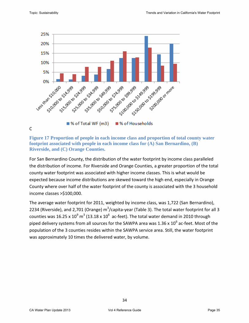
34
C
Figure 17 Proportion of people in each income class and proportion of total county water
footprint associated with people in each income class for (A) San Bernardino, (B)
Riverside, and (C) Orange Counties.
For San Bernardino County, the distribution of the water footprint by income class paralleled
the distribution of income. For Riverside and Orange Counties, a greater proportion of the total
county water footprint was associated with higher income classes. This is what would be
expected because income distributions are skewed toward the high end, especially in Orange
County where over half of the water footprint of the county is associated with the 3 household
income classes >$100,000.
The average water footprint for 2011, weighted by income class, was 1,722 (San Bernardino),
2234 (Riverside), and 2,701 (Orange) m3/capita-year (Table 3). The total water footprint for all 3
counties was 16.25 x 10⁹ m3 (13.18 x 10⁶ ac-feet). The total water demand in 2010 through
piped delivery systems from all sources for the SAWPA area was 1.36 x 10⁶ ac-feet. Most of the
population of the 3 counties resides within the SAWPA service area. Still, the water footprint
was approximately 10 times the delivered water, by volume.
Topic: Sustainability Trends and Variation in California's Water Footprint
CA Water Plan Update 2013 Vol 4 Reference Guide Page 35

35
Table 3. County-based 2011 water footprint calculation based on income, number of
households and number of people/household. Calculation made using the Water Footprint
Network’s Quick Water Footprint Calculator
(http://www.waterfootprint.org/?page=cal/waterfootprintcalculator_indv).
Orange Riverside San Bernadino
Average water footprint (m3/capita-year)
2,701 2,234 1,722
Total annual water footprint (m3/ac-feet)
8.2x10⁹/6.6x106 4.7x10⁹/3.8x106 3.4x10⁹/2.8x106
III.D. Discussion
Water Footprint is a useful meme to characterize both our dependence on water and our
impacts on water systems. Consumption of goods and services requires delivery of water
through natural and engineered pathways and return of wastewater to the environment.
Measuring uncertainty in water footprint calculations is useful because it helps to build
confidence in the footprint as a tool to inform decisions. It is also useful to find out how much
individual and collective water footprint can vary due to environmental and consumption
patterns because these patterns often involve choices. This means that people can decide to
change their water footprint by changing their consumption of water-intensive foods and
goods. It also means that decisions about crop production among sub-regions (e.g., within
California) can include information about water intensity, which provides a role for water
managers in improving sustainability of water use.
Agricultural production is the greatest contributor to an individual’s water footprint. We found
that variability in evapotranspiration of applied water among nine major crops resulted in the
water footprint of agricultural production ranging about 30% around the mean water footprint
across 4 years of analysis. This is a result of a combination of differences in water use for the
same crop in different places and at different times. If all other sources of variation were
ignored, then this variation would result in the California water footprint varying about
13%around the mean of 1,500 GPCD. This means that our estimate of the water footprint is
pretty good.
Another source of variation in water footprint is in individual choices for consumable goods and
services. One factor that seems to be a strong determinant of water footprint of consumption is
income, with people making more money tending to consume more goods and thus have a
larger water footprint (Hoekstra and Chapagain, 2007). To estimate the impact of variation in
Topic: Sustainability Trends and Variation in California's Water Footprint
CA Water Plan Update 2013 Vol 4 Reference Guide Page 36
36
income within California on calculated water footprint, we assumed that the influence of
national income levels on water footprint was approximately correct when used at finer scales,
such as for a county within California. Because there is variation in income in California and in
the US, as there is elsewhere in the world, it is useful to estimate water footprint using income
classes as one way to control for this variation. The Water Footprint Network has developed an
online calculator that estimates the water footprint based on income. This calculator was used
in combination with Census Bureau data to estimate the water footprints for each of the 3
counties that make up the SAWPA service region.
If households in California act similarly to households around the world, then one large source
of variation in water footprint will be rates and types of consumption, based on income. There
was at least an 8-fold difference between the estimated water footprint of the lowest income
class (household income <$10,000/year) and the highest income class (household income
>$200,000/year). This disproportionate makeup of the county water footprint was reflected in
the distribution of the water footprint by income class in Orange County, where >50% of the
water footprint is associated with household incomes >$100,000/year, despite the fact that
these groups make up <1/3 of the households. In contrast, San Bernardino County, which had
lower median household income and water footprint, displayed a more even distribution of
water footprint by income class.
Another factor causing variation in water footprint is diet, with vegetarian and vegan diets
having lower WF than meat-containing diets (da Silva et al., 2013; Vanham, 2013). This is
because it takes more water to produce meat than the caloric or weight-equivalent of
vegetables/grains. Using the Water Footprint Network’s online calculator, we found that for a
moderate individual income of $30,000/year a vegetarian diet resulted in a 27% lower water
footprint than a meat-containing diet. There is no similar calculator for a vegan diet, but it is
likely that the water footprint for a person with a vegan diet will be considerably lower than for
someone with a meat-containing or vegetarian diet.
A higher water footprint is both a greater impact on world water systems and a sign of
vulnerability. Maintenance of a high water footprint may not be sustainable in a water-
constrained world. Meat-based diet and higher income classes in the study area both had larger
water footprints than the county averages and global averages. These lifestyles may become
less sustainable with increased water limitations, or, if maintained, put unsustainable strain on
water limited systems.
IV. Issues, Data Gaps & Recommendations for Future Work
While the results provide a comprehensive analysis of California’s water footprint, the analysis
has several limitations. Using California-specific data presented several challenges in
Topic: Sustainability Trends and Variation in California's Water Footprint
CA Water Plan Update 2013 Vol 4 Reference Guide Page 37

37
incorporating these data into the water footprint methodology and in interpreting the results.
Trade data, particularly on the domestic level, is a limiting factor for developing an accurate
geographic picture of California’s water footprint. The different trade datasets used in our
initial assessment and in the present assessment also provided some variability in our results. In
particular, the resolution of SCTG (trade) categories, particularly in agricultural sectors,
introduces a significant amount of uncertainty about the composition of embedded water
imports and exports. We have also noted the need for more up-to-date and higher resolution
data on industrial water use, better separation of “withdrawals” versus “consumption” by
sector, and reconciliation of import and export reporting categories among state, national, and
international databases. For dietary and income effects on water footprint, we relied upon the
Water Footprint Network’s online calculator, which may not be inaccurate when applied within
a geographic region as it was applied here. Finally, better data are needed on the flow of goods
and services between regions inside California so that we can develop a better understanding
of how virtual water moves within and across regions. Despite these limitations, we believe
that our analyses provide important insight into the volumes and trends of California’s water
footprint as well as the issues that it presents for the state.
A water footprint assessment, by itself, provides limited information about the relative
advantages and disadvantages of relying on imports to support the state’s population. This
information, however, can be combined with a parallel assessment of water resource
conditions in those regions, today and in the future. Several groups have developed water
scarcity indices in an effort to compare water resource conditions around the world. For
example, the World Resources Institute (WRI) developed a water stress indicator for countries
and river basins around the world. Baseline water stress is defined as the ratio of the amount of
water withdrawn from a basin to the amount available from natural sources and imports
(Figure 18a).
Figure 18 provides a water stress index for every country and major river basin in 2025 and in
2095 under various climate scenarios. By 2025, most of the countries from which California
imports goods and services (Figure 2) will potentially experience some water stress. By 2095,
virtually all of the countries imported from and much of the mid-North American continent will
potentially experience water stress (Figure 3b).
Topic: Sustainability Trends and Variation in California's Water Footprint
CA Water Plan Update 2013 Vol 4 Reference Guide Page 38

38
a
b
Figure 18X. Baseline Water Stress in 2025 (a) and in 2095 (b) by Country.
Note: Darker colors are an indication of the greater likelihood that stress will be experienced
and the greater the severity of that stress.
Topic: Sustainability Trends and Variation in California's Water Footprint
CA Water Plan Update 2013 Vol 4 Reference Guide Page 39

39
The extent and severity of water stress indicated by these maps suggests risk to California’s
supply chain from global and US water stress. However, there are two big unknowns associated
with these kinds of projections. First, the projections are based on climate models, which have
their own uncertainties associated with them. Conditions may end up much worse or better
than indicated. Second, every country and US state that has trade relations with California has
their own priorities, based on local and regional needs and politics. As other regions become
stressed, how they respond in terms of trade and water-intensive production remains
uncertain. This combination of water and food insecurity is recognized by the US Department of
Defense as one of the greatest risks facing the U.S. (CITE/QUOTE?).
This analysis provides a comprehensive overview of California’s water footprint and how that
footprint varies temporally and regionally. The analysis, however, has raised additional
questions. In particular, we recommend the following studies for future work to address some
of the limitations of the current study:
Identify sources of applied water within California, such as distinguishing between
groundwater and various surface water supplies.
Explore ways to better integrate efficiency into water footprint analyses.
Evaluate how climate change will affect California’s water footprint.
Evaluate how California’s water footprint is expected to change in the future.
Evaluate California’s gray water footprint in more detail to obtain a better
understanding of past, present, and future water-quality concerns.
V. Citations
CDF CD of F (2011) California Population Estimates, with Components of Change and Crude Rates, July 1, 1900-2011. http://www.dof.ca.gov/research/demographic/reports/estimates/e-7/view.php.
CEC CEC (2013) Total Electricity System Power. http://energyalmanac.ca.gov/electricity/total_system_power.html. Accessed 29 Aug 2013
Coca-Cola Company and The Nature Conservancy (2010). Product water footprint assessments, Practical application in corporate water stewardship.
De la Rue du Can S, Hasanbeigi A, Sathaye J (2010) California Energy Balance Update and Decomposition Analysis for the Industry and Building Sectors.
daSilva, V., K. Maracaja, L. Araujo, J. Neto, D. Aleixo, J. da Cunha Campos. 2013. Water footprint of individuals with different diet patterns. Ambi-Agua, Taubaté, v. 8, n. 1, p. 250-262, 2013.(http://dx.doi.org/10.4136/ambi-agua.967)
Topic: Sustainability Trends and Variation in California's Water Footprint
CA Water Plan Update 2013 Vol 4 Reference Guide Page 40
40
EIA (US Energy Information Administration) (2012a) Annual Energy Review.
EIA EIA (2013a) California International and Interstate Movements of Natural Gas by State. http://www.eia.gov/dnav/ng/ng_move_ist_a2dcu_sca_a.htm. Accessed 29 Aug 2013
EIA EIA (2013b) Petroleum and Other Liquids: Company Level Imports. http://www.eia.gov/petroleum/imports/companylevel/. Accessed 29 Aug 2013
EIA EIA (2012b) Drought has significant effect on corn crop condition , projected ethanol production. Today in Energy
Fulton J, Cooley H, Gleick PH (2012) California’s Water Footprint. 53.
Gleick PH (2003) Water use. Annu Rev Environ Resour 28:275–314.
Gleick PH, Cooley H, Groves D (2005) California Water 2030 : An Efficient Future.
Hanak E, Lund J, Thompson B, et al. (2012) Water and the California Economy. 32.
Hoesktra, A.Y. and A.K. Chapagain. 2007. Water footprints of nations: Water use by people as a function
of their consumption pattern. Water Resources Management, 21: 35-48.
Jeffries, D., V.J. King, M.M. Aldaya, E. Ercin, A. Hoekstra, and L.M. Canals. 2009. Assessing water impacts of tea and margarine with a water footprint/LCA approach. Pilot study in Unilever. Presented at the LCA IX Conference, Boston, 9/29-10/2/2009.
Mekonnen M, Hoekstra A (2011) National water footprint accounts: the green, blue and grey water footprint of production and consumption, Value of Water Research Report Series No. 50 (Volume 2: Appendices).
Mekonnen M, Hoekstra A (2010a) The green, blue and grey water footprint of farm animals and animal products, Value of Water Research Report Series No. 48 (Volume 2: Appendices). UNESCO-IHE, Delft, the Netherlands
Mekonnen M, Hoekstra A (2010b) The green, blue and grey water footprint of crops and derived crop products - Volume 2 : Appendices.
Mekonnen M, Hoekstra A (2010c) The green, blue and grey water footprint of crops and derived crop products, Value of Water Research Report Series No. 47 (Volume 1: Main Report).
Meldrum J, Nettles-Anderson S, Heath G, Macknick J (2013) Life cycle water use for electricity generation: a review and harmonization of literature estimates. Environ Res Lett 8:015031. doi: 10.1088/1748-9326/8/1/015031
Topic: Sustainability Trends and Variation in California's Water Footprint
CA Water Plan Update 2013 Vol 4 Reference Guide Page 41
41
Orang MN, Snyder RL, Shu G, et al. (2013) California Simulation of Evapotranspiration of Applied Water and Agricultural Energy Use in California. J Integr Agric 12:1371–1388. doi: 10.1016/S2095-3119(13)60742-X
Rich J (2009) Comparing Changes in Applied Water Use and the Real Gross Value of Output for California Agriculture: 1967 to 2007. Water 4:3.
SAB Miller and World Wildlife Fund UK (2011). Water futures, Addressing shared water challenges through collective action.
SERI SERI (2011) Under Pressure: How our material consumption threatens the planet’s water resources. Vienna
Southworth F, Peterson BE, Hwang H-L, et al. (2011) THE FREIGHT ANALYSIS FRAMEWORK VERSION 3 (FAF3). Washington DC
USDA USD of AAMS (2001) GRAIN TRANSPORTATION REPORT.
USDC-BC UD of CB of C (2010) No Title.
USDC-BC UD of CB of C (1993) 1992 Census of Transportation , Communications , and Utilities.
USDC-BEA UD of CB of EA (2012) Regional Economic Accounts. http://www.bea.gov/regional/index.htm#gsp.
Vanham, D. The water footprint of Austria for different diets. Water Science and Technology, 67.4: 824-830 (doi: 10.2166/wst.2012.623)
Wu M, Mintz M, Wang M, Arora S (2009) Consumptive water use in the production of ethanonl and petroleum gasoline.
Topic: Sustainability Trends and Variation in California's Water Footprint
CA Water Plan Update 2013 Vol 4 Reference Guide Page 42