trends and patterns in crime: past, present, and … and patterns in crime: past, present, and...

U.S. Department Of Justice Office~of Justice Programs Bureau of Justice Assistance

, - - / ~6/%

Trends and Patterns in Crime: Past, Present, and Future..

West

Compilation and Revision of Materials Presented at BJA's ".lustice in the New Millennium" Regional Conferences

May -]une, 2000

PROPERTY OF National Criminal Justice Reference Service (NCJRS) Box 6000 Rockville, MD 20849-6000

If you have issues viewing or accessing this file, please contact us at NCJRS.gov.

U.S. Department Of Justice Office~of Justice Programs Bureau of Justice Assistance

Lt

~ 7

Trends and Patterns in Crime: Past, Present, and Future..

West

Compilation and Revision of Materials Presented at BJA's "Justice in the New Millennium" Regional Conferences

May - June, 2000

PROPERTY OF National Criminal Justice Reference Service (NCJRS) Box 6000 Rockville, MD 20849-6000

Trends and Patterns in Crime: Past, Present, and Future

Compilation and Revision of Materials Presented at

BJA's "Justice in the New Millennium" Regional Conferences

May - June, 2000

Prepared by

Community Research Associates, Inc.

William V. Pelfrey, Consultant Virginia Commonwealth University

November 2000

Bureau of Justice Assistance

810 7 th Street, NW Washington, DC 20531

(202)514-6278

Community Research Associates, Inc.

311 Plus Park Blvd., Ste 100 Nashville, TN 37122

(615) 399-9908

309 West Clark Street Champaign, IL 61820

(217) 398-3120

400 N. Columbus Street, Ste 205 Alexandria, VA 22314

(703) 519-4510

This project was supported by Cooperative Agreement No. 95-DD-BX-K001 awarded by the Bureau of Justice Assistance, Office of Justice Programs, U.S. Department of Justice to Community Research Associates, Inc. The Bureau of Justice Assistance is a component of the Office of Justice Programs. Points of view or opinion in this document are those of the author and do not necessarily represent the official position or policies of the U.S. Department of Justice and Community Research Associates, Inc.

Table of Contents

E x e c u t i v e S u m m a r y . . . . . . . . . . . . . . . . . . . . . . . . . . . . . . . . . . . . . . . . . . . . . . . . . . . . . . . . . . . . . . . . . . . . . . . . . . . . 1

I n t r o d u c t i o n . . . . . . . . . . . . . . . . . . . . . . . . . . . . . . . . . . . . . . . . . . . . . . . . . . . . . . . . . . . . . . . . . . . . . . . . . . . . . . . . . . . . . 11

C r i m e T r e n d s and Pa t t e rns :

N o r t h e a s t R e g i o n . . . . . . . . . . . . . . . . . . . . . . . . . . . . . . . . . . . . . . . . . . . . . . . . . . . . . . . . . . . . . 15

S o u t h e a s t R e g i o n . . . . . . . . . . . . . . . . . . . . . . . . . . . . . . . . . . . . . . . . . . . . . . . . . . . . . . . . . . .. 49

N o r t h C en t r a l R e g i o n . . . . . . . . . . . . . . . . . . . . . . . . . . . . . . . . . . . . . . . . . . . . . . . . . . . . . . . 83

S o u t h C en t r a l R e g i o n . . . . . . . . . . . . . . . . . . . . . . . . . . . . . . . . . . . . . . . . . . . . . . . . . . . . . . 119

West R e g i o n . . . . . . . . . . . . . . . . . . . . . . . . . . . . . . . . . . . . . . . . . . . . . . . . . . . . . . . . . . . . . . . . 151

M e t h o d o l o g y . . . . . . . . . . . . . . . . . . . . . . . . . . . . . . . . . . . . . . . . . . . . . . . . . . . . . . . . . . . . . . . . . . . . . . . . . . . . . . . . . 185

R e f e r e n c e s . . . . . . . . . . . . . . . . . . . . . . . . . . . . . . . . . . . . . . . . . . . . . . . . . . . . . . . . . . . . . . . . . . . . . . . . . . . . . . . . . . . . 191

Trends and Patterns in Crime: Past, Present, and Future

Compilation and Revision of Materials Presented at

BJA's "Justice in the New Millennium" Regional Conferences May - June, 2000

E x e c u t i v e S u m m a r y

In preparation for presentations at the "Justice in the New Millennium" regional conferences, existing datasets were identified, explored, collated, and assessed on crime, arrests, demographic projections, and social issues. These data were organized so that similar presentations could be made at Regional Conferences but tailoring the data to be specific to that region and the jurisdictions comprising it. The objective was to provide a snapshot of the past trends or patterns related to violent crime and drug use and comments of future trends or patterns. This was a daunting task but one which seemed imminently logical considering the topic for the Regional Conferences, Justice in the New Millennium. The manifest purpose was to provide clear, albeit general, information on crime and drugs in the jurisdictions. The latent purpose was to promote interest and enquiry into other ways of exploring, assessing, identifying and addressing issues such as crime and disorder, utilizing crime data but also utilizing social and demographic data in a fashion defensible based on criminological theory. For each of the regional presentations, crime and arrest data were used to describe the nature and extent of the problem and demographic data were used to describe projected changes in the jurisdictions. Together the two types of information provided defensible comments about the future.

Projections of demographic changes such as population growth, rates of change in the juvenile population, and race and ethnicity projections, are based on reasonably reliable information from governmental sources so there is a presumption of accuracy in these figures. Projections of social problems such as crime and drug use are much more problematic, however. The document concludes with a description of the Methodology used in these assessments. It is clear from the comments about limitations of the data that they are not as reliable or valid as we would prefer. They do however, in the absence of better, more reliable, more valid data, represent the most useful information reasonably available for such a project as this.

The main document has one section devoted to each of the five geographic Regions of the Bureau of Justice Assistance (BJA), State and Local Assistance Division. The conclusion of each section includes comments and observations on crime problems and drug problems, not in a statistical probability fashion, that would be guaranteed to be incorrect, but in a narrative description, based on the information assessed. The five

sections of the document are "Crime Trends and Patterns" in each of the BJA regions that are designated as the Northeast, Southeast, North Central, South Central, and West Regions. This Executive Summary also includes the concluding comments from each of the sections as well as general comments on the nation.

The format of each section of this publication is consistent with that of the regional presentations during the "Justice in the New Millennium" regional conference. There is redundancy in the format but the data and information for each section is tailored to apply to those jurisdictions within each region.

The objective for the regional presentations and the objective for this publication is to provide policy makers with the best, most current information on crime and drug use, as well as demographic projections which are likely to affect the jurisdictions, so that better, more appropriate plans can be derived from the data.

Violent Crime

Violent crime in the United States is lower than it has been in many years. The FBI's Uniform Crime Report for 1998, Crime in the United States notes "In 1998, the lowest national violent crime rate since 1985 was recorded .... " While this is an appreciated trend, there are still problems.

Most states have shared in the decline in violent crime seen in recent years. In observing trends in crime, however, it appears that there are states which have not participated in the same levels of decline or which still have unusually high rates of violent crime. Within each region, states will be discussed but it is important to view some patterns nationally.

The jurisdictions in the United States with the highest average violent crime rates from 1996 through 1998 were:

District of Columbia Louisiana Florida Illinois South Carolina California New Mexico Tennessee Maryland Nevada

These jurisdictions were identified by averaging the violent crime rates, per 100,000 population for the District of Columbia and each state in the Nation for 1996, 1997 and 1998. Average rates were used in an effort to "smooth" annual variations and gain a more accurate impression of levels of violence, as recorded by the Uniform Crime Reporting (UCR) Program. Violent crimes are defined as murder, rape, robbery, and aggravated assault, consistent with the UCR definitions. While each of the jurisdictions listed above had violent crime rate averages of 750 per 100,000 population or greater (the U.S. violent crime rate in 1998 was 566.4 per 100,000 population), the range was

significant among those jurisdictions. Nevada, with the lowest average of the top ten, had 751.24 violent index crimes per 100,000 population while the District of Columbia had more than 2,000 per 100,000 population.

Other jurisdictions had unusually high rates of certain violent crimes. The jurisdictions with the highest average murder rates for the three year period were:

District of Columbia Nevada Puerto Rico Maryland Louisiana New Mexico Mississippi

Each of these jurisdictions averaged more than l0 murders per 100,000 persons. It should be noted that all of these jurisdictions realized decreases in murder rates, comparing the average for the three years to the rate seen in 1998, except New Mexico that realized an increase in the murder rate from 1997 to 1998. Puerto Rico had an average murder rate of almost 20 per 100,000 population for the three year period but even that was low in comparison to the murder rate of the District of Columbia at 59.6 per 100,000 population.

Those jurisdictions with the highest average rape rates for the three year period were:

Alaska Florida Delaware Minnesota New Mexico Washington Nevada Tennessee Michigan South Carolina

For all of these states except Alaska and Delaware, the 1998 rape rates were lower than the three year average. As is stated in the text of the regional discussions of crime, there are reasons for rape rates to vary, other than sheer increases in criminal events.

Robbery rates were highest in the following jurisdictions, averaged over the period 1996 through 1998:

District of Columbia Puerto Rico

Maryland New York

These and most other jurisdictions have seen a decrease in robbery rates, however. Robbery rates and population density are positively and significantly correlated. This criminological fact may help in understanding the high rates of the jurisdictions listed here but, as described in the document, some sparsely populated jurisdictions have experienced high rates of robbery, suggesting that it is not a population density phenomenon at work but some more subtle issues serving as root causes.

3

Aggravated assault, comprising the bulk of violent crime rates in almost every jurisdiction, showed the highest averages in the following jurisdictions:

District of Columbia South Carolina Florida

New Mexico Louisiana

New Mexico's aggravated assault rates have increased consistently over the three year period, however. With its population growing more heterogeneous, a trait associated with difficulties in social control, growing at a rapid pace (42.5% from 2000 to 2025), and a growing proportion of juveniles, the state is likely to experience greater violent crime in the future. Florida's growth pattern shows a remarkable increase of 39.5% in its population from 2000 to 2025, but the juvenile proportion will decrease. This increase in total population, combined with ethnic heterogeneity, is likely to continue crime problems, either real or perceived (fear).

Generally, the District of Columbia represents the jurisdiction with the most serious violent crime problem in the Nation. It is, however, significantly different from almost every other jurisdiction due to its limited geographic size and the number of persons who travel into the jurisdiction daily. The population of the city is estimated at 523,000 but the population of the Metropolitan Statistical Area (MSA) is 4,629,510. When the MSA crime rates are considered, the area actually had a lower violent crime rate in 1998 than Wilmington, North Carolina. This does not, however, diminish the impact of high crime rates in the District of Columbia. The diversity of the population of the District of Columbia, described later, along with its poverty and juvenile population growth patterns over the next 25 years, suggest that crime will continue to plague the city, with social disorganization greater in the future than in the past.

There are some unusual patterns in crime rates discussed in subsequent sections. Puerto Rico has high rates of murder and robbery and the lowest rate in the nation for rape, but it is suggested that there must be some reporting issues associated with rape in the territory. Rural murder rates, for example, are extraordinarily high in New Mexico and South Carolina. Criminologists have offered some interesting and insightful explanations for the "narrowing of the gap" between urban crime rates and rural crime rates (See Weisheit and Donnermeyer, 2000). The demographic projections suggest that ethnic diversity and racial diversity will produce less homogeneous populations in those states, perhaps further challenging the rural areas to enjoy the diversity that the nation cherishes.

Drug Use

According to drug treatment data, treatment rates for drugs (other than alcohol) were highest in the following jurisdictions in 1997:

Connecticut Oregon Massachusetts Maryland Rhode Island

New York New Jersey District of Columbia Washington

4

The jurisdictions with high treatment rates, by drug category, varied significantly but it was evident from the data that the Western United States has experienced a significant influx of stimulant abuse. The rate, per 100,000 population, of treatment for stimulants is not as high as with some other drugs but the implications are serious, particularly with new drugs such as MDMA (methylenedioxymethamhetamine), known as "Ecstasy," becoming popular in a variety of settings. The growth and development of drug usage, as measured by treatment is discussed for each region but the implications to crime are serious.

Where drug use data suggest problems and crime data suggest problems, it appears that problems will be compounded. Such is the case with the District of Columbia. Crime data and demographic trend data, coupled with drug use, suggests serious problems for the jurisdiction.

Drug t r e a t m e n t data appear to be a better source of information on the nature and extent of drug use and abuse than arrest data, due to missing data in reported UCR arrest statistics and the policy issues associated with aggressive arrest strategies.

Demographic Changes and Patterns

Past crime rates combined with future demographic projections, may suggest some things about crime in the future. From 2000 to 2025, it is projected by the U.S. Census Bureau that California's population will increase 51.55 percent, Hawaii's population will increase 44.15 percent, New Mexico's 40.43 percent, Florida's 35.9 percent, Alaska's 35.53 percent and Texas' 35.11 percent. Some of these increases will be due to migration (particularly true of Florida) and some due to increases in different age groups. It is expected that those states with large increases in juvenile population, particularly juveniles aged 5 through 17, will experience increases in juvenile crime and juvenile victimization, although Zimring (1998) has insightful warnings on such projections.

The states with the largest increases in juveniles from 1995 to 2025 are:

Jurisdiction Increase in Juveniles 1995-2025 Total Population Change 2000-25 California 70.33% 51.55% Hawaii 59.62% 44.15% District of Columbia 55.41% 25.24% New Mexico 42.54% 40.43% Alaska 41.61% 35.53% Texas 38.21% 35.11% Arizona 35.01% 33.64%

Three of these jurisdictions currently have more than 53 percent of their children living in low income households (District of Columbia, New Mexico, and Arizona). Additionally, racial or ethnic diversity will cause changes in the social organization and structure of these and other jurisdictions. While Florida is not likely to lead the nation in percent of juveniles in the state, it will have significant total population growth over the next 25 years with an increase in the average age of its citizens. This will suggest other types of problems such as fear of crime.

Most of these states, as well as South Carolina, Maryland, and Louisiana, have experienced high rates of violent crime recently. It was suggested at the regional conferences that states prepare for the growth and diversity of each state's population so that change can be celebrated and welcomed.

Below are the major conclusions from each of the regional assessments. They are offered to provide a more panoramic view of the patterns that appear to be developing within the Nation and the regions.

Conclusions appropriate to the West Region:

Violent Crime has been and is likely to continue to be highest in New Mexico, particularly rural areas of the state and Albuquerque; metro areas of Nevada, particularly Clark County; Alaska, with a strong influence from alcohol use among juveniles; certain urban areas of California; and Multnomah County, Oregon;

In the next 25 years, due to growth and diversity, pressure will be placed on the justice system as an effective means of social control in Nevada, California, New Mexico, Alaska, and Hawaii;

Juvenile crime will be a significant factor in California, especially 2015-2025; Alaska and New Mexico, especially beginning in 2005; and Hawaii, throughout the next 25 years, due to increases in potential juvenile victims and offenders;

As juvenile-preferred drugs develop, especially in Western states, all drug use and abuse will have greater impact and influence on crime, including violent crime (particularly with stimulant use) and property crime (with other drugs);

New Mexico is likely to remain a major pocket of violent crime but California's population growth and heterogeneity is likely to produce increases in crime, including violent crime;

High rape rates in Alaska and high violent crime rates in New Mexico and Nevada, combined with drug abuse problems in Oregon, and dramatic growth in juveniles and Hispanic populations in California, suggest that the West Region is likely to be an area of concem in the future.

Conclusions appropriate to the Southeast Region:

Rural South Carolina counties, the District of Columbia, Puerto Rico, and the U.S. Virgin Islands are experiencing extraordinary levels of violence, particularly high murder rates and robbery rates;

The District of Columbia, Puerto Rico, Tennessee, and the U.S. Virgin Islands appear to have extremely high murder rates;

Florida, metro-Tennessee, and rural South Carolina have had high rape rates, among the highest in the Nation;

Rural South Carolina, the District of Columbia, and Florida appear to have the most significant violence problems in the region;

South Carolina's high level of alcohol abuse treatment suggests a relationship may exist between substance abuse and violence;

Dramatic growth in the population, combined with ethnic heterogeneity and an already high violent crime rate, are likely to impact Florida while poverty, racial heterogeneity and astounding levels of violence are likely to affect the District of Columbia;

Conclusions appropriate to the South Central Region:

Louisiana has experienced a violent crime problem that is significant and likely to continue. This violent crime problem includes high rates of murder and aggravated assault in the New Orleans area but also in the rural areas of the state;

The St. Louis area has significant juvenile murder and aggravated assault problems;

Oklahoma and Central Alabama have high rates of violence, with Oklahoma's violent crime problems almost certainly associated with drug use;

Ethnic diversity and astounding growth in Texas in terms of total population, juvenile population, and ethnic diversity as well as racial diversity and poverty in other South Central states, will contribute to social disorganization and increase the likelihood of higher levels of crime or disorder in the future;

Conclusions appropriate to the Northeast Region:

Murder does not appear to be a problem in the Northeast Region, except for unusually high rates in Maryland, where rape and robbery rates are also high;

Maryland and Delaware appear to have high rates of sexual assaults, as well as clusters of counties in Massachusetts and New Hampshire;

Aggravated assault rates were highest in Massachusetts but Maryland also has had high rates;

Heroin use and cocaine use appear to be highest in the Northeast Region, compared to all other regions;

Race and ethnicity, rather than population growth, are likely to be the leading reasons for change in the region over the next 25 years. These variables, combined with poverty measures and mobility, suggest that New York will recognize crime problems in the future, although there should be a reduction in juvenile crime due to a relative reduction in the proportion of juveniles.

Conclusions appropriate to the North Central Region:

Non-reporting through the UCR Program makes it difficult to recognize and interpret crime problems in some states in the North Central Region.

Other than Illinois, murder does not appear to be a problem in the region;

Rape appeared to be a problem only in Michigan and Minnesota, within the region, and it appears that rape rates will increase in the region, unlike any other region of the country. The increases in rape rates in Michigan, however, appear to be due in part or entirely to aggressive facilitation of reporting;

Illinois, particularly Cook County, has shown clear and consistent high levels of violence;

Minnesota has engaged in higher levels of arrests for drug sales while Wyoming has recorded higher rates of drug possession arrests. Michigan, Minnesota, and Ohio, however, have shown the highest levels of drug use, based on treatment data;

Illinois is likely to experience significant racial and ethnic changes in the next two decades, contributing to some social instability;

One piece of information is abundantly clear, and it applies to each region: data on reported crime and arrests are insufficient to judge the degree of the crime problem. Criminal justice planning is severely hampered by the lack of good, reliable, valid data on crime. It is recommended that states develop other measures of crime such as victimization surveys, in addition to reported crime, to better track the rates and locations of problems. Spatial analysis as well as the inclusion of social and demographic

8

variables may help to understand the nature and extent of crime and disorder. Clearly, good decisions require good data.

Introduction

"There is much crime in America, more than ever is reported, far more than ever is solved, far too much for the health of the Nation." This statement is certainly accurate today, even though violent crime has decreased remarkably in the recent past. We find ourselves at about the same level of violent crime as was experienced when this statement was printed on the first page of The Challenge of Crime in a Free Society: A Report by the President's Commission on Law Enforcement and the Administration of Justice in 1967. In 1968, because of the historically high levels of crime and violence, Congress passed the Omnibus Crime Control and Safe Streets Act. Our violent crime rates in the United States have now fallen back to those high levels that led to the passage of the most sweeping efforts to control crime. We can take little comfort in the knowledge that we have returned to those levels but with better information and better assessment, we may be able to understand the places and patterns posing the most serious crime risks. The belief that an analytical approach could contribute to an understanding of the crime picture, which could contribute to a more successful amelioration of the problems, was the basis for soliciting region-specific and state-specific presentations at the Regional Conferences of the Bureau of Justice Assistance (BJA), conducted during May - July, 2000. The Bureau of Justice Assistance has long stressed the importance of understanding and articulating the "Nature of the Problem" before considering strategies to address crime. The presentations sought to provide specificity regarding crime rates, crime regions, and expected problems based on future population trends. This publication captures the essence of the information provided in the conferences, as well as additional and revised information that became available subsequent to the Conferences.

Through invited, structured, organized presentations, workshops, and panels, BJA focused on Justice in the New Millennium as the theme for each of the five Regional Conferences conducted in May through July, 2000. A key element in addressing future justice, and crime, is establishing a nexus between the past, the present and the future. Each conference represented a subtle but serious model for strategic planning. Attendees participated in discussions on policy, planning, partnerships, technology, problems, analytical tools, tactics, and strategies. The crime problems, past and present, as well as demographic projections which may influence crime in the future served as the basis for one of the presentations at each conference and this document.

This publication is organized around the five BJA regions and the states comprising those regions. There is also a national component that focuses attention on the changes likely to occur in the population of the United States and the implications of those changes to the states and regions. While there is a clear preference to have all information reduced to state-level or even local level, crime, like most other social ills, is best recognized in reference and relationship to other jurisdictions. The use of regions is a defensible method of focusing, not for the purpose of drawing invidious comparisons but to recognize the arbitrariness of state boundaries in addressing crime, drug use, and violence. Where regions are used, generally, state-level information has been maintained so those reading this publication can draw their attention to the jurisdiction of greatest

11

interest. Performing intensive, specific assessments for every state, as has been done at the request of 18 states in the past several years, could not have been done on a timely basis for all 50 states, and the "Justice in the New Millennium" regional conference schedules could not have accommodated presentations with that degree of specificity.

Projections of demographic changes such as population growth, rates of change in the juvenile population, and race and ethnicity projections, are based on reasonably reliable information from governmental sources so there is a presumption of accuracy in these figures (See "Methodology" at the end of this publication for documentation and limitations of these data). Projections of social problems such as crime and drug use are fraught with errors, however. Since there is no statistically sound method for projection, any effort is likely to be wrong. Where there are suggestions of future problems, the comments are based on criminological foundations combined with historical information on crime patterns and projections of population dynamics, so they are believed to have some merit. But by raising the issues and making the suggestions, actions may be taken to head off the problems, thus nullifying the projections. That is the objective, not to be correct but to assist in equipping policy-makers with good information and reasonable inferences about the future so that actions may be considered to remedy problems. With that lofty objective in mind, we will address the nature and extent of violent crime and drug use in the five regions of the Untied States, then offer comments on the national trends and patterns. The BJA regions presumably were not defined based on cultural, social, or economic similarities but based on geography, contiguity, and caseload comparability within BJA. No effort has been made here to support or to challenge the organization of regions. Since they are identified, they will be used as an intermediate disaggregating criteria. Since the state-level information has remained intact, there appears to be no harm in whatever intermediate system is used to focus on trends and patterns. As stated in the Methodology, there are limitations to each set of data used but those data represent reasonable approximations of the issues being studied. With those caveats and disclaimers, what follows is one section devoted to each of the five geographic Regions of the Bureau of Justice Assistance, State and Local Assistance Division. There is also an Executive Summary that includes the observations and conclusions from each of the sections.

The format of this publication is consistent with that of the regional presentations during "Justice in the New Millennium" regional conferences. There is redundancy in the format but the data and assessments for each section are tailored to that region. The objective for the regional presentations and the objective for this publication is to provide policy makers with the best, most current information on crime and drug use, as well as demographic projections which are likely to affect the jurisdictions, so that better, more appropriate plans can be derived from the data.

The information contained in this document and discussed during the regional conferences certainly does not represent an ending point of assessment. It is more consistent with an intermediate method of describing problems and problem areas. A comment in the 1994 BJA publication, "Documenting the Extent and Nature of Drug and Violent Crime: Developing Jurisdiction-Specific Profiles of the Criminal Justice

12

System," describing the ground-breaking work of the Illinois Criminal Justice Information Authority to develop county-level profiles of the criminal justice system for each of Illinois' counties states:

"The data can be used to identify emerging problems or areas of need and as a tool to facilitate local-level discussions on how to take a systemwide approach to criminal justice planning."

Similarly, the maps prepared for the regional presentations and refined for this publication can serve as an elementary form of the spatial analysis needed to better target problems and problem areas. It should be stressed, however, that while these cross- sectional graphic displays are useful in recognizing possible problem areas or discrepancies between different data sources on drug use or arrests versus reports of crime, they can be made far more useful with state-specific data, described temporally as well as spatially. As stated by Anselin and others in a the recent National Institute of Justice publication, Criminal Justice 2000:

"Many of the capabilities to support computerized mapping and spatial statistical analyses emerged only recently during the 1990s. The promise of using spatial data and analyses for crime control still remains to be demonstrated and depends on the nature of the relationship between crime and place. If spatial features serve as actuating factors for crime, either because of the people who or facilities that are located there, then interventions designed to alter those persons and activities might well affect crime."

There may be many reasons for certain locations to appear to be "hot spots," as has been demonstrated in the discussions at the conferences and in the literature (See Sherman, et al., 1989). Discerning true problem areas demands location-specific data, over time, and location-specific knowledge of the attributes of the places.

Criminal Justice planners and decision-makers should find the methodology demonstrated here useful, even with all of the cautions regarding data and analyses. We strive to use the most reliable and valid data that are available. While there may be problems with those data, they still serve as our "best" measure of crime and disorder. This document utilizes Uniform Crime Reporting (UCR) Program data, both for crimes reported and arrests, as well as other data on social and demographic topics. Each dataset has limitations, some more than others, but the greater the variety of data and sources, the more likely it is that the true nature of the phenomenon will become evident. In addition to the variety of data shown here, there is the frequent comparison of jurisdictions to national rates or national standards. It is important to understand issues such as crime and disorder relative to some benchmark in addition to a particularly jurisdiction's past experiences. Finally, it is evident in this document that maps are preferred methods of displaying large datasets. Charts and tables can be just as useful, arguably more so for some purposes, but they cannot capture and display central foci as easily and as parsimoniously as maps. These preferences -- using diverse data to describe phenomena,

13

using rates and comparisons with benchmarks to determine relative standing, and using maps to present patterns-- are those of the author and were not prescribed by BJA. They have been useful in state-specific assessments of the nature, extent, patterns and trends in crime in more than one-third of the states in the past five years. It is suggested that readers refer to the "Methodology" section at the end of each regional discussion for more detail on the sources of the data and the limitations, but give consideration to conducting state-specific assessments similar to the regional assessments presented here.

There may certainly be some frustration in not finding concrete "projections" of crime in this document. Zimring (1998) has stated forcefully and convincingly that there is no single trend for all violent crimes but trends, where they exist, are crime-specific. There are better, more complete discussions of future crime patterns such as a variety of chapters included in Criminal Justice 2000. An introductory chapter by LaFree et al. (2000: 20), includes an instructive comment:

Probably the only safe predictions that can be made about future violent arrest and crime rates, juvenile or otherwise, are that they are unlikely to return to the low levels witnessed in the 1950s and early 1960s, and that the declines witnessed in the early 1990s, most dramatically in several large cities, are unlikely to continue.

Some patterns are discemable from the data and assessment presented in this document. It is clear that violent crime has been higher in certain areas of the nation and, based on demographic shifts, some states and regions are more likely to experience future crime problems. Only with further, more specific assessment, grounded in criminological explanations (See, for example, Tittle, 2000, for an excellent discussion of criminological explanations and research), will more accurate pattems and trends become evident.

14

Crime Trends and Patterns Northeast Region

Maine

New York

Pennsylvania

The Northeast Region of the United States, as defined by BJA, consists of the following states:

Connecticut New Jersey Delaware New York Maine Pennsylvania Maryland Rhode Island Massachusetts Vermont New Hampshire

The U.S. Census Bureau estimates the current population of the states comprising the region to total 58,125,000 persons. The average of the median income for each of the states in the region for 1998 was $41,580, according to the Census Bureau, Housing and Household Economic Statistics Division. The average median income in the region, by state, for 1996 through 1998 ranged from a low of $34,989 in Maine to a high of $49,303 in New Jersey. The median income average for the United States for the period was $37,779.

The total land mass for the eleven states in the Northeast Region is 174,003 square miles. The population density for this region is 334 persons per square mile.

15

Index Crime Rates in the Northeast Region I

The crime rate trends for index violent crimes in the Northeast Region compare favorably with the U.S. averages. "Index crimes" reported are defined by the Federal Bureau of Investigation, Uniform Crime Reporting Program (UCR, 1998: 5):

The Crime Index is composed of selected offenses used to gauge fluctuations in the overall volume and rate of crime reported to law enforcement. The offenses included are the violent crimes of murder and nonnegligent manslaughter, forcible rape, robbery, and aggravated assault, and the property crimes of burglary, larceny-theft, motor vehicle theft, and arson.

Our focus here is on violent crimes so only the first four are described. In order to compare crimes across jurisdictions, it is necessary to convert the number of crimes to some standard format. The generally accepted measure used in crime analysis is "crimes per 100,000 population" where the population statistic is the estimated population for reporting jurisdictions for each year considered. For the general tables shown below, the UCR (Uniform Crime Reporting Program) data were estimated for non-reporting jurisdictions but with the county level data, non-reporting jurisdictions are excluded for all except arrest data.

Murder

M u r d e r R a t e s 1 9 9 1 - 9 8

1 2

1 0

8

6

4

2

0

m u s

- - Nm- the~as l

UCR Data, R a t e s p e r 100,O00 population

Murder (including nonnegligent manslaughter) represents the most serious but rarest of crimes in the crime index. As the chart above shows, the Northeast Region has had and continues to have, a lower rate of murder than the average for the U.S. The average murder rate for the Nation in 1998 was 6.3 per 100,000 population while the average murder rate for the eleven states comprising the Northeast Region was 4.78 per 100,000 population. The national average murder rate was the lowest recorded since 1967.

Some of the states within the region had exceptionally low murder rates, according to an analysis of UCR data. New Hampshire had an extraordinary murder rate of 1.52 per

'See "Methodology" section at the end of the document for data sources, limitations and methods used.

16

100,000 population, about one-fourth the U.S. average. Similarly, Maine and Massachusetts had murder rates of about 2 per 100,000 population, one-third the U.S. average. In fact, all of the states except one had murder rates below the U.S. average for 1998. The exception was Maryland with a murder rate of almost 10 per 100,000 population, about 63 percent higher than the U.S. rate. Maryland's murder rate was highest in the metropolitan areas of the state.

As with most social issues, murder rates were not equally distributed in or among the states. As the map below shows, Baltimore and Prince George's County had high rates in Maryland while Atlantic County in New Jersey showed higher than average rates. Baltimore had the highest murder rate in the region with 47.56 murders per 100,000 population. The Philadelphia area, including Camden, NJ had very high rates.

Murder Rate 1998 Rates per 100,000 Population

r-] 6.2 to 47.6 (26) [ ] 3.1to 6.2 (53) [ ] 0 to 3.1 (165)

New York City had higher than average rates and the adjacent counties in New Jersey, Hudson and Essex, shared in the high murder rates. Other counties in the region showed the isolated presence of high rates, such as Maine's Washington County, New Hampshire's Merimack County and Pennsylvania's Cameron and Elk Counties.

Juvenile violence is a particularly troubling issue for many jurisdictions. Within the Northeast Region, however, it appears that juvenile arrests for homicide are isolated. Baltimore and Dorchester County, Maryland had juvenile arrest rates for murder that were among the highest in the region. Philadelphia's juvenile murder rate was less than half that of Baltimore. Fulton County, New York had the highest juvenile arrest rate for murder in the region for 1998.

17

Juvenile Murder Arrest Rat( . . . . R ~ s per 10~,0~0 P o p ~

[ ] 2.5to 7.51 (7) [ ] 0.5to2.5 (37) [ ] 0 to0.S (2OO)

Care should be exercised in interpreting rates for one year in sparsely populated areas. Single year anomalies do not suggest a pattern and serve simply as a warning that patterns might develop. With Baltimore data, however, 51 juveniles were arrested for murder in 1997 and 43 were arrested for murder in 1998 in a jurisdiction with almost 700,000 persons. These figures do suggest a pattern of high rates of juvenile murder.

The Northeast Region county map compares favorably to the national map regarding murder rates, per 100,000 population. As the map below shows, this region, when juxtaposed with the rest of the United States, appears not to have a murder problem.

18

.81.

"%

U~ W~bbld~

U.S. Murder Rates by County 1998 Rates per 100,000 ~ i o n

D 6.31o134 (650) [ ] 1.3to 6.3 (647) [ ] o to 1.3 (1846)

Similarly, state-wide rates support the impression that murder is generally not a problem in the Northeast Region. Maryland represents the exception to that impression.

1998 Murder Rates Rates per 100,000 pOl~ion

D 82to49.8 (8) [ ] 6 to 6~. (16) [ ] o to 6 (29)

L ...... I == I co,o~o I ...... S. "~'i .K_./ ?'~',,

P~n~ Rico

The historically low rate of murder in the Northeast region, actually decreasing at a faster pace than the U.S. rates, suggests that the rate is likely to continue to decrease in the region. The chart below shows the regression line, based on past rates.

19

Regional Projected Murder Rates

~0~

~4

a4

7J

0 4

41 go

Murder Rates Northeast Region 1991-98

Observed and Projected

m o Observed

o Une l l ,

. P fo l ec t t d i

99

The trend lines projected and observed are quite consistent and the slope is significant.

As stated earlier, murder is the most serious of crimes reported to police, and it is the one most likely to be reported when it occurs. The reliability and validity of the statistic makes it one of the best measures of violence, based on official statistics (there are more valid methods of measuring other crimes than official statistics). Since it is a relatively rare event, it becomes difficult to determine pattems or trends in areas with low populations since a few crimes can cause unusual spikes in rates. It appears, based on historical information, that murder is not generally, and will not generally be a problem in the Northeast. Maryland, particularly Baltimore, and areas surrounding Philadelphia and New York City are jurisdictions which have shown above-average rates in homicide.

Rape

Just as murder is one of the crimes most likely to be reported when it occurs, rape is one of the most underreported crimes. Since there is a gap between the actual number of forcible rapes occurring (or attempted) and those reported to police as having occurred or attempted, it is sometimes difficult to determine whether high rape rates mean more rapes occur or more of the rapes that occur are being reported. The crime is certainly a serious one and regardless of the interpretation, the data should be studied and the degree of the problem assessed. Later there will be recommendations on how best to judge the trend or pattern of rapes reported to police.

As was true of murder, the Northeast Region has rape rates that are and have been far below the U.S. average. As the chart below shows, the states of the Northeast Region had forcible rape rates more than 30 percent lower than the U.S. average.

20

Rape Rates 1991-98 45

4O ~ " ~ 3S

30 ~ - - - ~ ' ~ - ~ , . ~ _

25 - ~ - ' - -

20

15

10

- - U S

- - N o r t h e a s t

UCR Data, Rates per 100,000 population

In 1998, the U.S. average for forcible rape rates was 34.4 per 100,000 population while the average for the region was 25.1 per 100,000 population. There have been no unusual spikes or valleys in the trend line for the region and the rates have decreased at about the same slope as the national rates.

When unusual spikes appear in the rates of sexual assaults reported to police, over time, for a jurisdiction such as a state, it may suggest an extraordinary increase in sexual assaults or, arguably, it may suggest an aggressive and effective effort to facilitate reporting of the crime when it occurs. Victim Assistance Coordinators, Rape Crisis Centers, and persons within prosecutor offices may be effective in reducing the gap between the number of crimes occurring and the number of crimes reported. On a regional basis, it appears that there are no unusual pattems in the data so the supposition is that the data reflect the same rate of reporting, year after year.

State-level rape rates show that Delaware had a rape rate of 67.07 per 100,000 population for 1998, a rate far higher than any other state in the region. In fact, that rate was the second highest in the nation. The 1998 UCR warns, however, that the number of rapes in Delaware was estimated from information furnished by the state. The data furnished by the state-level UCR program were found not to be in accordance with UCR guidelines so rates in local jurisdictions are not available. Only the state total is available. This is why the counties in Delaware do not reflect high rates in the map below.

21

e Rates by County 1998 ,000 population

) 81.8 (38) ) 39 (S2)

~ ..~21.9 (124)

This map shows that there are pockets of higher than average rape rates within the Northeast Region. Maryland, particularly Baltimore but also all of the counties contiguous to Delaware reflected high rates, as did Cumberland, Cape May and Camden Counties in New Jersey. Essex County New Jersey in the New York City area also had high rape rates. New London County, Connecticut, and clusters of counties in Massachusetts and New Hampshire, reflected high rape rates in 1998.

As was mentioned in the BJA Regional meetings, jurisdictions with colleges and universities sometimes have higher than average rape rates. Again, this may be due to campuses facilitating the reporting of assaults or it may be due to a higher frequency of occurrence. One other statistical explanation might be the increased non-residents (for Census purposes) on or around campuses on a semi permanent basis contributing to the number of potential victims but not included in the denominator in calculating the crime rates. Arguably, population alone is not the most significant factor; otherwise all crime rates would appear higher in those jurisdictions.

As the U.S. map below shows, there are pockets of high forcible rape rates throughout the Nation, including the Northeast Region. Again, this map excludes Delaware Counties since those data were not available.

22

U.S. Rape Rates by County 1998 Rates per 100,O0O population

[ ] 39 to 986 (650) [ ] 21.9to 39 (651) [ ] 0 to 21.9 (1842)

On a state-wide examination, the Northeast Region, except for Delaware, appears to have low forcible rape rates, compared to other states. While all of the states in the region except Delaware have rape rates well below the U.S. average, the range is significant. Maine had the lowest rape rates in the region in 1998, with 18 per 100,000 population. New Jersey was the next lowest state with an average of 20 per 100,000 population. New York and Connecticut were the only other states in the region with rates below the regional average of 25 per 100,000 population in 1998.

Rape Rate 1998 Rate~ per 100,000 pol0t~ion

[ ] 49 to 68.6 (7) [ ] 38to49 (13) [ ] Oto3S (32)

J

\ \ .. . . . . I .... I co,~o I ~, .... ~ , , ,o~ ~ _ 2 " 4 " ,j 'o,, , ,~,

r - - - - x

2 3

Delaware clearly had the highest rate in the region with 67 per 100,000 population and the next highest was Rhode Island with 35.5 per 100,000, New Hampshire with 33.76 and Maryland with 33.38 per 100,000 population.

As was the case with murder, the trend line for rape in the Northeast Region is strongly declining.

Regional Projected Rape Rates Rape Rates Northeast Region 1991-98

Observed and Projected 32,

3 t j

3o4

2o,I

2sJ

274

2O4

2~4

241 90 g l 92 gO ~4 g~ g~ g7 @8

o Observed

a Unus

m Projected

Again, this trend line, based on regression, appears consistent with the national trend and this line would have rather accurately predicted the rape rates over the past six years.

Robbery

While some states consider robbery a "crime against property," the Uniform Crime Report and the accepted definition of the crime place it within the category of violent crimes. Robbery is predominately an urban crime, and historically the highest rates have been found in metropolitan areas and densely populated jurisdictions.

As the chart below shows, the Northeast Region has experienced higher than average robbery rates although the gap is narrowing. The U.S. robbery rate in 1998 was 165 per 100,000 population. The rate was significantly higher, 198 per 100,000 population, for metropolitan areas of the Nation. The robbery rate in the Northeast Region in 1998 was 195 per 100,000 population. Two states, New York and Maryland, exceeded that regional average with state rates of 270 and 298 per 100,000 population. Vermont, on the other hand, had a robbery rate of 9.48 per 100,000 population in 1998 and Maine and New Hampshire each had rates of 21 per 100,000 population.

24

Robbery Rates 1991-98 400

350

300

250

200

150

I00

50

0

m u s

Northeast Region


Even though the Northeast has had robbery rates higher than the U.S. average, the rate of decline has been steeper and the highest rates have been restricted to very few jurisdictions.

This restriction is evident in the map below showing the county-specific robbery rates for 1998.

~er,/Rates by County 1998 0,000 population

1 ,I 70 (71) 62.S (7O)

v ..~ 20.9 (103)

25

Those counties along the east coast and within the most densely populated areas of the region had the highest rates of robbery. It should be noted that the ranges for this map and the robbery maps for other regions use relatively low rates, even for the highest range. This is done to show where, within each region, the rates are highest and may be useful in assessing drug-related offenses as well. Robbery is one of the crimes frequently associated with drugs and, while it cannot serve as a proxy for drug use, may help to focus attention on a serious violent crime which may also serve to reduce drug-related offenses.

Nationally, the Northeast Region reflects more "hot spots" than was seen in previous crime maps, as reflected in the map below.

U.S. Robbery Rates by' County 1998 R~es per 100,000 population

17 62.6 to 3,230 (651) [ ] 20.9 to 62.8 (652) [ ] 0 to 20.9 (1840)

o,,~5=

The U.S. map depicting the rates for robbery by state show New York and Maryland as being among those states with the highest robbery rates. According to UCR analysis of robbery rates, the Northeastern States (the FBI does not use the same group of states to form the Northeast Region as does BJA so exact comparisons are not possible) have far higher incidents of robberies on streets or highways, and lower rates of commercial house robberies or gas/service station robberies.

26

Robbery Rate 1998 Rates per 100,000 ~ i o n

[ ] 190to S,.qO (9) [ ] 140to190 (11) [ ] 0 to 140 (32)

, ~ ..... J 10~,o : L ~ . , , ~ ~

Pt~nR Rico

Again, the robbery rate trend line, as reflected by the regression line, is strongly downward. Based on this projection, the robbery rates in the Northeast Region of BJA are likely to be at or below the U.S. averages within the next two years.

Regional Projected Robbery Rates

Robbery Rates Nodheas t Region 1991-98


l o .... "~Proje~td

27

Aggravated Assault

Aggravated Assault, an assault often accompanied by the use of a weapon, is the most frequently occurring of the serious violent crimes. The U.S. average for aggravated assault in 1998 was 360.5 per 100,000 population. While the average for the Northeast Region was lower than the national average in 1998, several states within the region had unusually high rates.

As the table below shows, the Northeast Region has had and continues to have lower than average aggravated assault rates. This is due, in part, to some extraordinarily low rates in two states. New Hampshire had an aggravated assault rate of 50.4 per 100,000 population in 1998 and Vermont had a rate of 67 per 100,000 population. Delaware, on the other hand, had an aggravated assault rate of 498.3 per 100,000 and Massachusetts had a rate of 495.3 per 100,000 population. Maryland also had a high rate of 454.5 per 100,000 population in 1998.

Aggravated Assault Rates 1991-98

$00

450 - - - ~ 400

550

3 0 0

250 200

150

100

$ 0 I

.... ~ U $

~ N o r t h e a s t Region


Clearly, the distribution of aggravated assault rates varies significantly. As the map below shows, there are pockets of violent, serious assaults within the region.

28

;ault Rates by County 199B population

0 (41) 5.9 (60)

t.~ . . . . . 0.2 (143)

The two obvious pockets of violence are the Maryland and Delaware combination and Massachusetts. Delaware's rural counties had an average aggravated assault rate of 615 per 100,000 population for the 101,111 citizens who lived in those jurisdictions.

/ -

° o "

U.S. Aggravated Assault Rates by County 1998 Rates per 100,000 population

I-I 345.9 to 13,090 (650) [ ] 180.2.to 345.9 C650) [ ] 0 to 180.2 (1843)

The national county-level map above shows that there are clearer, more obvious pockets of aggravated assault in other regions and the pockets described earlier are somewhat hidden because of the geographic concentration of counties in the Northeast.

29

Aggravated Assault Rates 1998 Rates per 100,000 population

[ ] 495 to 944 (8) [ ] 3 5 0 t o 4 9 5 (11) I-7 0 to 350 (,33)

Montana s ~ C r ' ~ ~ ~

I . . . . I . . . . . . I t Ohio, Net=Jersey

¢---t

Push.Rico

The state-level map above shows clearly that Maryland, Delaware, and Massachusetts are among those in the top tier of states with high aggravated assault rates. Again, the rates are declining in the Northeast and the Nation.

Regional Projected Aggravated Assault Rates

Aggravated Assault Rates Northeast 1991-98

Observed and Projected 400

38O

340

32~ g Observed

o Line,mr

3~0 "=~Pmjeded ~0 91 Q2 QC3 04 ~ (~ g7 g8 99

This projection of the regression line shows the decline of aggravated assault in the Northeast Region and suggests that the decline will continue. The states and counties representing pockets of violence, however, should not be masked by this trend.

30

Drug Use in the Northeast Region

One of the issues of importance to the Bureau of Justice Assistance and the states is the use of illegal drugs. Assessing the use of drugs is even more problematic than assessing the incidence of crime. Drug arrests have, historically, been one of the major indices of drug presence in a jurisdiction, even though estimates are used widely (See Methodology). Drug interdiction and drug arrests are, however, clearly tied to resources and policy decisions. Drug enforcement is proactive enforcement. If a jurisdiction has resources, human and otherwise, to focus on drug arrests, arrests occur thus proving the presence of drugs. If a jurisdiction lacks sufficient resources to proactively address drug possession and drug sales, the lack of arrests might spuriously suggest the absence of illegal substances. Similarly, policy decisions often determine the location of proactive drug enforcement. If drug arrests occur in a neighborhood, community, or school, it certainly means there were drugs present in those locations. If, however, no proactive enforcement occurs in a neighborhood, community, or school and no drug arrests are made, it does not necessarily mean that there were no drugs present.

Even with those caveats, it would be inappropriate to ignore drug arrests as some indication, incomplete as it is, that drugs are present in certain locations. The UCR categories for drug arrests include two major categories possession and sales/manufacture. Within each category the types of drugs are specified: marijuana, opiates, synthetic opiates, and "other." What is described here is arrest rates, by county, for all drug offenses, drug possession, and drug sales/manufacture. Other data will be shown regarding types of drugs.

As the map below shows, drug arrests in the region are concentrated along the Maryland, Delaware, New Jersey, New York corridor, extending farther north into Connecticut. While Massachusetts has two jurisdictions in the highest category, it is New York State's Central, Western, Northern and Southeastern sections, along with Southern New Jersey, Maryland and Delaware that show the strongest presence of drugs, based on total arrests. Notably absent in the high categories are counties in Pennsylvania.

31

: Rates 13y County 1998 )00 popu~ion

0 (S2) 6.9 (74)

_ 1.3 (108)

When considering drug possession arrests in 1998, virtually the same pattern is present. This is not unusual since most arrests for drug crimes are arrests for possession. The map below shows the same corridors and concentrations.

rrest R a t e s ~ County 1998 i pop~aUon

(70) 5 (TS) 3 (gg)

Drug sales and manufacture arrests represent, arguably, more serious issues than possession. Many agencies, including BJA, have been encouraging greater attention be paid to these offenses.

32

As the map below shows, the pattern of arrests for drug sales and manufacture are very different from those of possession.

ares by County 1998 p~l~lon

s3) 97) g4)

As the map rather clearly shows, Eastern Pennsylvania, Maryland, Delaware, New Jersey, and the New York City area are those most associated with drug sales arrests. New York State's other regions, while high in possession arrests, are not as engaged in drug sales arrests. This observation is not intended to be a critique. Many issues fit into the decisions to engage in certain types of proactive enforcement.

While drug-crime arrests may serve as an indication of the presence of drugs, they may not be as useful in understanding the relative use of drugs. Arrests certainly do not suggest the absence of drugs. Other data may be useful in better understanding drug use.

33

Almc,~

TEDS 1997 Drug Treatment Rates Rates per 100,000 poptz~ion

[ ] 100to191 (9) [] 50to10O (2:2) [ ] 0to 50 (21)

" R ~ d = It, land

C=mlin=

The map shown above depicts drug treatment rates, per 100,000 population, gathered by Substance Abuse and Mental Health Services Administration, U.S. Department of Health and Human Services. The data is prepared and published by the Office of Applied Studies as the "Treatment Episode Data Set" (TEDS). The TEDS system is described as one which (OAS, 1999: 3):

Comprises data on treatment admissions that are routinely collected by states in monitoring their individual substance abuse treatment system. Selected data items from the individual State data files are converted to standardized format consistent across States. These standardized data constitute TEDS.

TEDS includes, as the unit of analysis, treatment admissions to substance abuse treatment facilities receiving federal funding. Typically, these facilities include public and private nonprofit programs. Absent are data from for-profit treatment programs. Alcohol treatment is included as "substance abuse treatment" and represents the bulk of treatment in almost all programs. Since there is an interest here in illegal drug use, alcohol treatment has been removed from the data presented. The map above reflects treatment rates for all illegal drugs.

The highest rates for drug treatment in 1997, the most recent year for which data were readily available, were observed in Connecticut, Massachusetts, Maryland, Rhode Island, New York, and New Jersey, in order from highest rates (190.9 per 100,000 population in Connecticut). Rhode Island only had one jurisdiction appear in the highest category of drug arrest rates and that was Providence for drug sales arrests, yet the state was one of the highest treatment states in the region, suggesting the use of drugs was occurring.

34

.9,,

TEDS 1997 Heroin Treatment Rates Rates per 100,000 population

[ ] 40 to109 (8) D 7.51o 40 (10) D 0 to 7.5 (34)

/ ~ , "== ~ ~ ~ ll>,, ' ,~', ' l ,8~-- ':"

The map above shows the rates of treatment for heroin use, according to TEDS for 1997. The Northeast Region is the major cluster of the nation regarding heroin treatment. Within the region, treatment rates were highest in Massachusetts (105.2 per 10,000) and Rhode Island (104.4 per 100,000) for heroin use. The next highest states were New Jersey and Maryland.

Below, we see the states with the highest rates of treatment for cocaine and crack cocaine. Connecticut, New York and Maryland were the states with the highest rates of treatment for cocaine and crack cocaine use in 1997. As with heroin, the Northeast represents a cluster of use of cocaine, joined by the states of Ohio and Michigan.

35

> Ab,.~a

TEDS 1997 Cocaine Treatment Rates Rates per 100,000 population

[ ] 35 to 57.6 (7) [ ] 18to 35 (16) [ ] otole (29)

Ida,la,l~ M~n D a ~ i

-@ There is no presentation here of a map depicting stimulant use in 1997 since the rate of use in the Northeast was very low. It appeared not to represent a problem for the region or the states in the region.

It is suggested that TEDS represents a viable corollary to arrest data in understanding the presence of drugs within certain jurisdictions. It was surprising to note the high rtes of heroin and cocaine use in Connecticut and the high rate of drug treatment, particularly heroin treatment, in Rhode Island. These data help to better understand drug use as well as enforcement strategies.

Social and Demographic Issues in the Northeast Region 2

As this Nation enters the Twenty-first Century, major shifts are occurring in social and demographic factors. Of course, all of the shifts are continuations of trends established in preceding decades but the impact of some of the changes will be evident in crime.

In succeeding issues of the annual report on crime published by the Federal Bureau of Investigation, the agency comments in the introductory remarks to Crime in the United States (1999:iv):

Historically, the causes and origins of crime have been the subjects of investigation by varied disciplines. Some factors that are known to affect the volume and type of crime occurring from place to place are:

Population density and degree of urbanization.

2 See "Methodology" section at the end of the document for social and demographic data sources, limitations and methods used in this assessment.

36

Variations in composition of the population, particularly youth concentration. Stability of population with respect to residents' mobility, commuting patterns, and transient factors. Economic conditions, including income, poverty level, and job availability. Cultural factors and educational, recreational, and religious characteristics. Family conditions with respect to divorce and family cohesiveness. Climate. Effective strength of law enforcement agencies. Administrative and investigative emphases of law enforcement. Policies of other components of the criminal justice system (i.e., prosecutorial, judicial, correctional, and probational). Citizens' attitudes toward crime. Crime reporting practices of the citizenry.

Some of these issues have been addressed earlier in this document, such as enforcement emphases and resources of law enforcement. Others such as rates of juveniles in jurisdictions are obviously important in understanding crime rates and victimization. Criminological theory and research support the notion that there are many factors influencing crime. One of the theoretical approaches which has proven to be quite robust over the past seven decades and which is useful in explaining crime in particular places is "Social Disorganization" theory. Generally, the three components of the approach are:

Heterogeneity Mobility Poverty

There are many other approaches that could be used to describe why and where crime rates are likely to be high (see Tittle, 2000). However for the Regional BJA presentations of 2000, "Social Disorganization" elements, combined with other variables, were presented as important components in assessing crime. This is not a test of the theory or even a concerted effort to address the theory. The research does serve as a rationale for including certain variables in the presentations and those descriptions are used here. Rather than an ex post facto description of crime and various elements, what is presented here is a description of some past but more future projections of social and demographic patterns and trends, in hope of anticipating issues facing regions, states and jurisdictions.

Heterogeneity, Growth and Change in the Northeast Region

The Nation is realizing significant change in its citizenry. This change will continue but, like crime, change is not equally distributed. The elements of greatest change revolve around race, ethnicity and age. These components may be considered "heterogeneity" although most of the research suggests race and ethnicity as the key elements.

One of the things that make this Nation great is its diversity. We celebrate racial, ethnic, and cultural diversity and consider it an attribute. Criminological research suggests that change, including change in race and ethnicity, can negatively impact the social

37

organization of communities. Ethnic and racial heterogeneity are described here in an effort to recognize the change that is likely to occur and accommodate, welcome, and assimilate the change in such a manner that it does not contribute to disorganization.

.elaska /

Ethnic Diversity 2025

1"7 0.34 to 0.5 (7) [ ] 0.22to034 (6) [ ] 0 too.~ (39)

I zanl e~v ~ x [ ¢ o

Texas i '

Ethnic diversity is based on the formula (1 - ~aoo) where p is the proportion of the population in each of the categories of Hispanic and Non Hispanic. Racial diversity, described below, is based on the same formula but where p represents the proportion of persons in each of the racial categories. These formulas were used by Warner and Pierce (1993) in applying social disorganization theory to crime data.

Ethnic diversity, shown in the map above, is likely to be greatest in regions other than the Northeast however New York, New Jersey, and Connecticut are projected to show strong increases in the proportion of the Hispanic population through the year 2025. It is projected by the Census Bureau that by 2005, Hispanics will represent 16 percent of the population of New York, 14 percent of the population of New Jersey, and 10 percent of the population of Connecticut. By 2015 the Hispanic population in those states will have increased to 19 percent in New York, 17 percent in New Jersey, and almost 13 percent in Connecticut. Additionally, Rhode Island is expected to have Hispanics representing 12.4 percent of its population by 2015. By 2025, almost one-quarter (21.7 percent) of the population of New York will be Hispanic, 19.5 percent of New Jersey and more than 15 percent of Rhode Island and Connecticut will be Hispanic.

Racial diversity, shown in the map below, will affect much of the Nation, including the Northeast Region states. By the year 2025, it is expected that the Asian and Pacific Islands racial category will represent about l0 percent of the population of New York and New Jersey. It is projected that by 2025 one-third of the citizens of Maryland will be black and more than 20 percent of the citizens of New York will be black.

38

Hl~li

Racial Diversity Scores 2025

[ ] 0.34 to 0.54 (17) [ ] 0.22to0.34 (17) [ ] 0 to0.22 (18)

The combinations of racial diversity and ethnic diversity will have greatest effect on the states of New York and New Jersey, within the Northeast Region. It is imperative that, among other things, these states insure that their criminal justice agencies and other governmental agencies reflect the diversity of the population.

In the next series of maps, the change in the juvenile population is described. The Census Bureau projects that the nation's youth will account for a smaller proportion of the population in 2025 than in 1995. Within the Northeast Region, Maryland is expected to see a growth of 17 percent in the number of persons aged 5 through 17 by the year 2025. This growth rate will be greatest from 2015 through 2025. Delaware will see an increase in juveniles through 2005 then the growth will slow remarkably. New Jersey and Massachusetts will also see a growth in juvenile population from 2015 through 2025. By 2025 juveniles will represent about 16 percent of the population with the highest proportions in New York (18 percent) and Maryland (17 percent).

39

Nevad;

, i I%

Percent Change in Juvenile Population 1995-2005

[ ] 15 to25.7 (6) [ ] o tols (31) [ ] -asto o (is)

=h e=k~ ",, 7,£-~. ,/:'-I .I-/',:/ -:~

ona ,,o Me~i¢ ~ rkans Camlin

,I


[ ] 15 to38.8 (11) [ ] 0 tolS (21) [ ] -13.7to 0 (20)

Rtco

40


[ ] 15 to70.4 (17) [ ] 0 to15 (21) [ ] -17.5to 0 (14)

Momana I 3. ~z's¢'~ ~x....,-~ P i ~ n n e s ~ I . ~ - - " M a i / r~4

fA ' , j

~ah l~are

ona

Mobility in the Northeast Region

Mobility is represented by data collected by the Census Bureau on domestic migration (migration from state to state) and international migration (migration from other countries). Only two states in the region have experienced increases in domestic migration in the past decade. Those states, Vermont and New Hampshire, have recognized relatively small increases of .95 percent to 2.46 percent. New York has lost 10.38 percent due to domestic migration while Connecticut has lost 6.9 percent and Massachusetts and New Jersey about four percent each.

41

Nevad

Changes in Population due to Domestic Migration 1990-99 ~ s Expressed in Percentages

[ ] 5.2to 24 (11) [ ] -o.sto 5.2 (21) [ ] -28.3to-0.5 (20)

1,~ ~ o~o,~ " ' ~ - _ ~ana

• Maine

i , ~ . A - - : - . i t - - ~ t ' ~ ' " = ' ° ' l t , _ , . . . , / f l e w I ; , la ,mp.~hire

i ......... r- ~ o=~ ~ ) _ _ j . J t 7 - T - - - - - ~ "--~,,.,~,.I I o~o, ,,=J,N~

¢k n Carolln ~ona . ~ a s etu MeIIo

PU~;~ Rico

The map below shows that international migration has benefited New York. The state has recognized a gain of more than six percent due to international migration, the second highest gain in the nation.

,e "J~

.40=

Nevad

Population Change 1990-99 clue to International Migration Claarxje Expressed es Percentages

I - ] 2 to 6.88 (17) I - I o.r4 to 2 (17) [ ] 0 to0.74 (18)

/ o ~ l m a I S

.oral ew MeJiO ~r~

Population growth rates, while not directly due to "mobility," do represent change. Presumably the change is advantageous since growth is generally preferred to decline,

42

but rapid or remarkable change must be recognized and proactive steps taken to accommodate it.

The maps below show the population growth expected through 2025.

According to the U.S. Department of Commerce, the states of California, Texas and Florida are likely to recognize the greatest increase in population through 2025. It appears that the net gain of those three states from 1995 to 2025 will be over 32 million persons. California alone will increase by almost the entire expected population of New York.

~¢aska I Populat ion Change Projected f rom 2000 to 2005

Change Expressed as Percentage Increase

[ ] 7.5to10.7 (6) [ ] 5 to 7.5 (12) [] o to 5 (3,i)

M0a~at~

I " [ I . . . . . . . . . I ~ i/ i~lcnl~lan I ~,..,..,..~l Nelil Hiir~$him

From the pattern shown in these maps, it appears that the West will lead the growth. Five western states are expected to grow by more than 50 percent from 1995 to 2025.

43

/~aska

Population Change Projected from 2000 to 2015 Change Expressed in Percentage Increase

[ ] 15 to27.3 (15) [ ] 7.5 to 15 (21) [ ] 0 to 7.S (16)

Montana /~ t o ~ ° ~ - ' F - - - - - q so=h o,k=, I ~ . . . . YP.. L ~ ; ~ Nero H~t~shire

1 I I I I Nebraska ~, '~" ~ " ~ . Connecticut

t t " ~ ' ° " ° I utah I ~.~^~,~^ I ~. X . . . . . . r ~ "=L , I "0i~ttI'~'0f Columbi+

ao ~

Northeast states will grow but at a far slower pace. By the year 2025, shown in the map below, Maryland will have recognized an 19 percent increase in total population, compared to the year 2000. This will be the highest percentage of growth in the region. New Hampshire and New Jersey will see an increase of about 17 percent followed by Rhode Island that will recognize an increase of 14 percent. The smallest gain in the region and the third smallest in the Nation will be in Pennsylvania with an increase of less than 4 percent.

~aska l

J@

Montana

Population Change Projected from 2000 to 2025 Change Expressed in Percentage Increase

[ ] 15 to 51.6 (29) [ ] 7.5to 15 (17) [- I o to 7.s (s)

10f Cotumbl~

44

Poverty

By its very nature, poverty is a very quantifiable variable. According to the literature, however, it is not as much the poverty rate as the disparity between the poor and the wealthy which may be most influential in crime and violence. What is presented below are two measures of poverty. The first, shown in the map below, is the three-year average percentage of children living at or below 200 percent of the U.S. poverty level. This is generally referred to as "Percent of Children in Low Income Homes." The rate for each state is averaged for the three year period.

As a region, the Northeast had a rather low percentage. The U.S. percentage was 42.2 while the Northeast Region had 36.6 percent of its children living in homes at or below that income level. New York had the highest percentage, 44.5 percent, with Maine, Delaware, and Pennsylvania following. The lowest percentage was seen in Maryland with only 27 percent of children living in low income households.

Average Percent of Children in Poverty, 1996-98

[ ] 43.8to60.2 (17) [ ] 36.1to43.8 (17) [ ] 0 to36.1 (18)

• t~l/~ Rico

The other measure suggested here, as a proxy for economic deprivation, is the Gini Index. The most recent year for which data are available by state is 1989. Each year the U.S. Department of Commerce samples persons throughout the nation to arrive at a U.S. Gini Index but the sample size is insufficient to estimate state indexes any years except full census years. Again, New York had the highest rate in the region with an index of .467. The Gini Index seeks to measure the disparity between the wealthiest and the poorest. The higher the index score, the greater the disparity between the wealthiest and the poorest in a jurisdiction.

45

Nevad

GINI Scale for Households 1 g89 [ ] 0.439to0.492 (17) [ ] 0.42 to 0.439 (1 7) [ ] 0 to0.42 (18)

'hlco'o °o I . . . .

Texas I , iSJ

~ PuL;~ P:s¢o

One other measure of "community stability" was proposed during the presentations. That measure was the voting rates during major elections. While it is certainly not suggested as a variable directly associated with crime, it may serve as a proxy for community activism and may indicate the degree to which community-oriented initiatives might be acted upon.

Within the region, voting rates in the 1996 election were highest in Maine where, of those registered, 70 percent of women and 68.5 percent of males voted. Lowest rates were seen in Pennsylvania, Maryland, and Delaware.

Concluding Comments on the Northeast Region

Murder does not appear to be a problem in the Northeast Region, except for unusually high rates in Maryland, where rape and robbery rates are also high;

Maryland and Delaware appear to have high rates of sexual assaults, as well as clusters of counties in Massachusetts and New Hampshire;

Aggravated assault rates were highest in Massachusetts but Maryland also had high rates;

Heroin use and cocaine use appear to be highest in the Northeast Region, compared to all other regions;

Race and ethnicity are likely to be the leading reasons for change in the region over the next 25 years. These variables, combined with poverty measures and

46

mobility, suggest that New York will recognize crime problems in the future, although there should be a reduction in juvenile crime.

47

Crime Trends and Patterns Southeast Region

m l

Tennessee

Virginia ~ ; ~

Georgia

~ o O ~ Viro~l~land~

The Southeast Region of the United States, as defined by BJA, consists of the following jurisdictions:

District of Columbia Florida Georgia North Carolina Puerto Rico

South Carolina Tennessee U.S. Virgin Islands Virginia

The U.S. Census Bureau estimates the current population of the states and territories comprising the region to total 51,920,000 persons. The average of the median income for each of the states in the region for 1998 was $35,860, according to the Census Bureau, Housing and Household Economic Statistics Division.

The total land mass for the nine jurisdictions in the Southeast Region is 275,302 square miles. The population density for this region is 188.59 persons per square mile. The range of population density in the region is tremendous, however. The District of Columbia, consisting of 61.4 square miles, with a population of 523,000 produces a population density of more than 8,500 persons per square mile. Puerto Rico and the Virgin Islands, have a population density of about 1,000 persons per square mile while South Carolina has a population density of 133.9 persons per square mile.

49

Index Crime Rates in the Southeast Region 3

Thecrime rate trends for index violent crimes in the Southeast Region show the region as having higher rates of violent crimes, compared with the U.S. averages. "Index crimes" reported are defined by the Federal Bureau of Investigation, Uniform Crime Reporting Program (UCR, 1998: 5):



Murder

Murder Rates 1991-98

10

8

6

4

I

m u s

S o u t h e a s t

Region


Murder and nonnegligent manslaughter represents the most serious but rarest of crimes in the crime index. As the chart above shows, the Southeast Region has had and continues to have, a higher rate of murder than the average for the U.S. The average murder rate for the Nation in 1998 was 6.3 per 100,000 population while the average murder rate for

3 See "Methodology" section at the end of the document for data sources, limitations and methods used.

50

the nine jurisdictions comprising the Southeast Region was 9.2 per 100,000 population, almost 50 percent higher than the U.S. average. The national average murder rate was the lowest recorded since 1967.

The only jurisdiction with murder rates close to the U.S. average was Virginia, with a murder rate of 6.21 per 100,000 population in 1998. Florida's murder rate of 6.48 per 100,000 population was the next highest with all other jurisdictions at or above 8 murders per 100,000 population in 1998. The District of Columbia recorded almost 50 murders per 100,000 population and Puerto Rico had almost 18 murders per 100,000 residents. Data for the U.S. Virgin Islands are not precisely comparable and are not presented here. It appears, however, that that territory's violent crime rates are among the highest in the region, per 100,000 population.

As with most social issues, murder rates were not equally distributed in or among the jurisdictions. The map below shows graphically that many counties within the region were above the U.S. average murder rate in 1998. Among the most populous jurisdictions, the District of Columbia had the highest rate of 49.7 murders per 100,000 population and Richmond, Virginia was close to that high with 48.45 murders per 100,000 population. North Carolina, South Carolina, and much of Florida had counties with high murder rates for 1998. Care should be taken in interpreting single year rates however.

Southeast Region Murder Rates by Court1 Rates per 100~00 p o ~

I"1 6.3to 134 (210) I--I 1.3to 6.3 (171) I--I 0 tO 1~(273)

__rlo Rico

l~b U.S. Virgin Islands

Fulton County Georgia, Robeson County, North Carolina, and Orangeburg County, South Carolina, and Davidson County, Tennessee all had murder rates in 1998 that were more than three time the U.S. average and all three had significant populations suggesting that a single-year assessment is not likely to be an aberration. Additionally, these counties and jurisdictions all had high murder rates in 1997. Sparsely populated counties showed high rates but unless data for preceding years were inspected, it would be inappropriate to

51

<:3

t~

suggest that these represented patterns of problems. It is important to note, however, that rural counties in South Carolina, collectively, had an average murder rate that was almost 40 percent higher than the state's average. These data suggest that, while the state as a whole did not have the highest murder rate in the region, the rural areas are experiencing a significant problem.

The Southeast Region county map does not compare favorably to the national map regarding murder rates, per 100,000 population. As the map below shows, this region, when juxtaposed with the rest of the United States, appears to have a significant murder ~roblem.

U.S. Murder Rates by County 1998 Ra~es per 100,00~ population

[ ] S.3 to 134 (SSO) [ ] 13to 6.3 (647) [ ] 0 to 1.3 (1646)

"~" ¢t

Similarly, state-wide rates support the impression that murder is a serious problem in the Southeast Region. As stated earlier, only Virginia and Florida had murder rates at about the U.S. average, although both appear in the intermediate level in the map below. Additionally, all of the other jurisdictions were at or above 8 murders per 100,000 population, with District of Columbia, Puerto Rico, Virgin Islands, and Tennessee have the highest rates.

52

1998 Murder Rate Rate per 100,000 ~ i o r l

[ ] 8.2to49.8 (8) [ ] 6 to 8.2 (15) [ ] O to 6 (29)

Mor4ana nes

Oh~ rsey

' ~ , Texa

The rate of murder in the Southeast region has decreased, although sporadically, but the trend line suggests that the rate is likely to continue to decrease in the region. The chart below shows the regression line, based on past rates.

Regional Projected Murae~ Murder Rates Southeast Region 1991-98

Observed and Projected 115 e.

"°1 =1 Inn

95

911

8 5

B

m ° P II~¢IRO

: Rates

53

The trend lines projected suggests that murder rates in the region are likely to decrease, although the rates in the past have shown inconsistency.

As stated earlier, murder is the most serious of crimes reported to police, and it is the one most likely to be reported when it occurs. The reliability and validity of the statistic makes it one of the best measures of violence, based on official statistics (there are more valid methods of measuring other crimes than official statistics). Since it is a relatively rare event, it becomes difficult to determine patterns or trends in areas with low populations since a few crimes can cause unusual spikes in rates. It appears, based on historical information, that murder is a significant problem in the Southeast, and will continue to show rates higher than the U.S. average. The states of South Carolina (particularly rural South Carolina), North Carolina, and portions of Florida and Tennessee, as well as the District of Columbia, and the U.S. territories appear to have the greatest murder problems.

Rape

While murder is one of the crimes most likely to be reported when it occurs, rape is one of the most underreported crimes. Since there is a gap between the actual number of forcible rapes occurring (or attempted) and those reported to police as having occurred or attempted, it is sometimes difficult to determine whether high rape rates mean more rapes occur or more rapes are being reported. The crime is certainly a serious one and regardless of the interpretation, the data should be studied and the degree of the problem assessed. Later there will be recommendations on how best to judge the trend or pattern of rapes reported to police.

As was true of murder, the Southeast Region has rape rates that are and have been higher than the U.S. average. As the chart below shows, the states of the Southeast Region had forcible rape rates higher than the U.S. average and the gap has not closed appreciably.

54

Rape Rates 1991-98 5O

4 5 / ~

3 5 - - ' ~

3O

2 5

2 0

15

10 I , ,

~ U S

~ S o u t h e a s t

R e g i o n


In 1998, the U.S. average for forcible rape rates was 34.4 per 100,000 population while the average for the region was 39.7 per 100,000 population. There have been no unusual spikes or valleys in the trend line for the region and the rates have generally tracked the national rates.

When unusual spikes appear in the rates of sexual assaults reported to police, over time, for a jurisdiction such as a state, it may suggest an extraordinary increase in sexual assaults or, arguably, it may suggest an aggressive and effective effort to facilitate reporting of the crime when it occurs. Victim Assistance Coordinators, Rape Crisis Centers, and persons within prosecutor offices may be effective in reducing the gap between the number of crimes occurring and the number of crimes reported. On a regional basis, it appears that there are no unusual patterns in the data so the supposition is that the data reflect the same rate of reporting, year after year.

State-level rape rates show that Florida had a rape rate of 49.6 per 100,000 population for 1998, a rate higher than any other state in the region. Tennessee had the second highest rate in the region with 45.8 rapes per 100,000 population. Tennessee's rape rate has decreased remarkably from 1997 when it had one of the highest rates (56.9 per I00,000) in the Nation. Even though Florida and South Carolina saw rape rates decrease slightly from 1997, the rates were still far higher than the U.S. average.

As the map below shows, there were clearly pockets of high rape rates. In South Carolina, again, the rural rates were extremely high. In fact, the rural rape rates in South Carolina and Florida were the highest in the region. The metro rape rates in Tennessee were the highest in the region (57.3 per 100,000 population).

55

Southeast Region Rape Rates by County 1! R~des per 100,000 population

[ ] 39 to117 (144) [ ] 21.9to 39 (177) [ ] 0 to 21.9 (283)

__ .'to Rico I ~¢ r , - -L

~lb U.S. Virgin Islands

This map shows that while there are pockets of higher than average rape rates within the Southeast Region, there are some areas with exceptionally high rates but that do not form clusters. Shelby County and Davidson County Tennessee both had rape rates in 1998 that exceeded 90 per 100,000 population. This means that almost two of every 1,000 women were "sexually assaulted in those jurisdictions in 1998. Hamilton County Tennessee and Duval County Florida also had unusually high rape rates in 1998.

As was mentioned in the BJA Regional meetings, jurisdictions with colleges and universities sometimes have higher than average rape rates. Again, this may be due to campuses facilitating the reporting of assaults or it may be due to a higher frequency of occurrence. One other statistical explanation might be the increased non-residents (for Census purposes) on or around campuses on a semi permanent basis contributing to the number of potential victims but not included in the denominator in calculating the crime rates. Arguably, population alone is not the most significant factor, otherwise all crime rates would appear higher in those jurisdictions.

As the U.S. map below shows, there are pockets of high forcible rape rates throughout the Nation, including the Southeast Region. South Carolina and Florida show consistent patterns of high rape rates.

56

'2"

a,' ¢t

U.S. Rape Rates by County 1998 I%t•s per 100,080 populatk~

[ ] 39 to 986 (650) [ ] ~ .gto 39 (SSl) [ ] 0 to 21.9 (1842)

On state-specific examination, the Southeast Region, except for Florida, South Carolina and Tennessee, appears to have relatively low forcible rape rates, compared to other states. Puerto Rico had the lowest rape rate in the region in 1998, with 6.3 per 100,000 population. Considering the high rate of violence shown in murder rates, there may be a reporting issue in which victims do not readily report sexual assaults to police in that jurisdiction. Otherwise, there must be some explanation for the low rates. The other four states in the region ranged from 26.7 rapes per 100,000 population in Virginia to 36.3 in the District of Columbia. Again, Virgin Islands data were not compatible with those of the other jurisdictions but it appears that the rape rates were higher than the national average.

57

R a p e R a t e 1998 Rates per 100,000 popu~ion

[ ] 49 to 68.S (7) [ ] 36to 49 (13) [] 0to36 (32;)

iru

ey

As was the case with murder, the trend line for rape rates in the Southeast Region is declining but the decline is not as consistent as is seen in other regions.

Regic nal Projected Rape Rates Rape Rates Southeast Region 1991-98


t4

~J go 91 g~ 93 94 95 96 g? 96

o t ~ t i

o GIm~

58

Robbery

While some states consider robbery a "crime against property," the Uniform Crime Report and the accepted definition of the crime places it within the category of violent crimes. Robbery is predominately an urban crime, and historically the highest rates have been found in metropolitan areas and densely populated jurisdictions.

As the chart below shows, the Southeast Region has experienced higher than average robbery rates since 1993 and the gap is widening. The U.S. robbery rate in 1998 was 165 per 100,000 population. The rate was much higher, 198 per 100,000 population, for metropolitan areas of the Nation. The robbery rate in the Southeast Region in 1998 was 215 per 100,000 poPulation. The District of Columbia far exceeded the U.S. average with a robbery rate of 689.5 per 100,000 population. Puerto Rico had a robbery rate of 296.6 per 100,000 and Florida's robbery rate was 242.7 per 100,000 population in 1998. Virgin Islands' robbery rate also appeared to be higher than the U.S. average. The other states had robbery rates ranging from 105.6 in Virginia to 187.2 in Georgia.

Robbery Rates 1991-98 300

250

200

150

100 '

5 0

.

- - U S

Southeas t R e g i o n


The Southeast has had robbery rates higher than the U.S. average and the rate of decline has been shallower for the region.

It should be noted that the range of rates for robbery in the map below are not consistent with the highest range being higher than the U.S. average. Robbery is an urban crime

59

and many states have low rates. The range was selected to show pattems. It appears that North Carolina, South Carolina, and large portions of Tennessee and Georgia show those pattems.

Southeast Region Robbery Rates by Cou: RaCes per 100,000 ~ r to Rico

20~qto 6 ~ (179) [ ] 0 to 209 (t72) ~=, U.S.Virginlstan@s

I

Below are some of the rates of robbery, per 100,000, reflected in the map above for 1998: Rate Jurisdiction 704.01 Fulton Georgia 689.48 District of Columbia 631.37 Richmond, Virginia 525.36 Durham North Carolina 518.65 Dade Florida 518.21 Portsmouth, Virginia 506.55 Shelby Tennessee 418.83 Davidson Tennessee 414.11 De Kalb Georgia 393.74 Mecklenburg North Carolina 368.37 Hillsborough Florida 363.09 Petersburg, Virginia 320.55 Hamilton Tennessee 318.60 Norfolk Virginia 313.04 Orange Florida 305.40 Madison Tennessee 296.57 Puerto Rico 293.23 Wilson North Carolina 291.13 . Guilford North Carolina 290.40 Dougherty Georgia 288.42 Duval Florida 286.19 Palm Beach Florida

60

Those counties and cities shown above are among the most densely populated areas of the region, validating the proposition that robbery is an urban crime. Again, it should be noted that the ranges for this map and the robbery maps for other regions use relatively low rates, even for the highest range. This is done to show where, within each region, the rates are highest and may be useful in assessing drug-related offenses as well. Robbery is one of the crimes frequently associated with drugs and, while it cannot serve as a proxy for drug use, may help to focus attention on a serious violent crime which may also serve to reduce drug-related offenses.

Nationally, the Southeast Region reflects more "hot spots" than was seen in previous crime maps, as reflected in the map below. Not surprising, based on other crime rates, South Carolina's rural counties had higher rates of robbery than other states rural areas.

~e

/

0

Dmt~ili==

U.S. Robbery Rates Ioy County 1998 Rates per 100,0~) population

[ ] 62.8 to 3,230 (651) [ ] 20.9to 62.8 (652) 1-] 0 to 20.9 (1840)

The U.S. map below depicting the rates for robbery by state show District of Columbia, Puerto Rico, and Florida as being among those states with the highest robbery rates.

61

Robbery Rate 1998 Rates per 100,000 population

[ ] 190 to690 (9) [ ] 140to190 (11) [ ] 01o140 (32)

I OId=homa

io ~ Texas

~a rsey Ire

~ o

Again, the robbery rate trend line, as reflected by the regression line, is downward but the slope is less remarkable than that of the U.S. averages. Based on this projection, the robbery rates in the Southeast Region of BJA are not likely to be at or below the U.S. averages within the foreseeable future.


Robbery Rates Southeast Region 1991-98

Observed and Projected 3W

62

Aggravated Assault

Aggravated Assault, an assault often accompanied by the use of a weapon, is the most frequently occurring of the serious violent crimes. The U.S. average for aggravated assault in 1998 was 360.5 per 100,000 population. The average for the Southeast Region was higher than the national average in 1998 and several states within the region had unusually high rates.

As the table below shows, the Southeast Region has had and continues to have higher than average aggravated assault rates. The 1998 rate in the Southeast Region was 482.5 per 100,000 population, more than 30 percent higher than the U.S. average of 362 per 100,000. The trend line has been consistent with that Of the U.S. average, only much higher. This is due, primarily, to three jurisdictions, the District of Columbia, South Carolina, and Florida. Only Puerto Rico, Virginia, and Georgia (by a slight margin) have rates lower than the U.S. average.


6 0 0 '

5 0 0 '

4 0 0 '

5 0 0 '

I

2 0 0

100 '

0 ' ] I I I

- - U S

- - S o u t h e a s t

R e g i o n


Clearly, the distribution of aggravated assault rates varies significantly. As the map below shows, there are pockets of violent, serious assaults within the region. Two of these pockets could general be described as South Carolina and Florida. Additionally, corridors in North Carolina and Tennessee show high rates of aggravated assault.

63

<3i

B

Southeast Region Aggravated Assault Rate Rate~ per 100,000 population

[ ] 345.9 to 7,040 (234) [ ] 150.2to 345.9 (175) [ ] 0 to le0.2 (lSS)

__.to Rico L.._,Cr--t

U.S. Virgin Islands

Rural South Carolina is, once again, well represented among the jurisdictions with high rates. Rural aggravated assault rates in South Carolina in 1998 were 690 per 100,000 population, almost four times the U.S. average for rural jurisdictions and higher than the aggravated assault rates in urban areas of South Carolina. Additionally, Davidson County Tennessee and Fulton County Georgia had high rates in 1998.

"%

U.S. Aggravated Assault Rates by County 1 998 Rates per 100,050

[ ] 345.9 to 13,000 (650) I-I lS02to 345.9 (650) 17 0 to 180.2 (1843)

°

c,,~itl._~q k :o

64

The national county-level map above shows that there are obvious pockets of aggravated assault in many regions including the counties in South Carolina, North Carolina, Florida and portions of Tennessee the Southeast.

Aggravated Assault Rate 1998 Rates per 100,000 population

[ ] 49sto 944 (8) [ ] 350to495 (11) D oto 3 ~ (33)

I Ok lahoma I

a u~

SOUn LPseY

f

The state-level map above shows clearly that South Carolina, Florida, and the District of Columbia are among those in the top tier of states with high aggravated assault rates. Again, the rates are declining more slowly in the Southeast compared to the Nation.


Aggravated Assault Rates Southeast Region


a¢l

~ i l a ~ e R . a

65

This projection of the regression line shows the decline of aggravated assault in the Southeast Region and suggests that the decline will continue somewhat. It is expected that 1999 rates will be higher than 1998 rates.

Drug Use in the Southeast Region


Even with those caveats, it would be inappropriate to ignore drug arrests as some indication, incomplete as it is, that drugs are present in certain locations. The UCR categories for drug arrests include two major categories - possession and sales/manufacture. Within each category the types of drugs are specified: marijuana, opiates, synthetic opiates, and "other." What is described here is arrest rates, by county, for all drug offenses, drug possession, and drug sales/manufacture. Other data will be shown regarding types of drugs.

As the map below shows, drug arrests in the region are concentrated in Georgia, South Carolina and portions of Tennessee. Almost every county in Georgia and South Carolina was in the highest or intermediate level of arrest rates for 1998, the most recent year for which data are available. Complete arrest data were not available to the UCR from Florida so no arrest data are included for that state.

66

Southeast Region Drug Arrest Rates by Col Arrest rates per 100,000 population

[ ] 506~q to 2.930 (214) [ ] 301.3to 513S.9 (157) [ ] 0 to 301.3 (233)

__.,to Rico

U.S. Virgin Islands


Southeast Region Drug Possession Arrest Arrest redes per 100,1~010o~

D 3~7.sto2~90 (lm) [ ] 225.6to 397.6 (174) [ ] 0 to 22s.s t~oo)

__;to Rico I - - . . .a_I

~, U.S. Virgin Islands


67

As the map below shows, the pattern of arrests for drug sales and manufacture are not remarkably different from those of possession.

Southeast Region Drug Sales Arrest Rates Arrest rates per 100,000 10o¢~lstk

I-I 100.Stol,010 C23S) [ ] 43.6to 100.8 C150) [ ] 0 to 43.6 (219)

__.to Rico

U.S. Virgin Islands

As the map rather clearly shows, Georgia, South Carolina and Tennessee are fully engaged in arrests for sales as well as possession. North Carolina, however, shows a higher concentration of arrests for possession than for sales. This observation is not intended to be a critique. Many issues fit into the decisions to engage in certain types of proactive enforcement.


68

AIm=a

hlcca~

n"

,e ~"%

TEDS 1997 Drug Treatment Rates Rates per 100,000 population

[ ] 100to191 (9) [ ] 50to1~]~ (22) [ ] 0to 50 (21)

Na,~n I)==uta U a n ~ , = k(i

~ n 1 ¢ ~ isr.at.i a t , i e l Ot Calum ala

r b , i ~

The map shown above depicts drug treatment rates, per 100,000 population, gathered by Substance Abuse and Mental Health Services Administration, U.S. Department of Health and Human Services. The data, prepared and published by the Office of Applied Studies as the "Treatment Episode Data Set" (TEDS). The TEDS system is described as one which (OAS, 1999: 3):



The highest rates in the Southeast for drug treatment in 1997, the most recent year for which data were readily available, were observed in the District of Columbia (112 per 100,000 population). The next highest rates of treatment were seen in South Carolina (64 per 100,000) and North Carolina (62 per 100,000). Although alcohol treatment is not included in this map or this analysis in general, it should be noted that South Carolina had an unusually high rate of treatment for alcohol use, according to TEDS. The alcohol use in South Carolina may very well be associated with the high levels of violent crime in that state.

69

AIm4=

Ida

,o 0"~,

TEDS 1997 Heroin Treatment Rates Rates per 100,000 population

[ ] 40 to109 (8) [ ] 7.5to 40 (10) [ ] 0 to 7.5 (34)

T~n,m.n~m

The map above shows the rates of treatment for heroin use, according to TEDS for 1997. The Southeast Region shows virtually no heroin use, as of 1997, except of the District of Columbia. The data from the Drug Abuse Warning Network (DAWN) however, show that there has been an increase in Emergency Room visits in Miami attributable to heroin u s e .

Below, we see the states with the highest rates of treatment for cocaine and crack cocaine. The District of Columbia, North Carolina, and South Carolina were the jurisdictions in the region with the highest rates of treatment for cocaine and crack cocaine use in 1997. The treatment rates for DC were in the highest category and those for North Carolina and South Carolina were at the upper limit of the intermediate range.

70

,o ~"¢b

TEDS 1997 Cocaine Treatment Rates Rete~ per 100,00010opulat~n

D ~tosT~ co [] ~sto~ o6) [] oto~e (29)

fa ~

j ~

I

P ~ F ~

There is no presentation here of a map depicting stimulant use in 1997 since the rate of use in the Southeast was very low. It appeared not to represent a problem for the region or the states in the region. Only slight levels of treatment were observed in Georgia in 1997.


Social and Demographic Issues in the Southeast Region 4





71

Population density and degree of urbanization. Variations in composition of the population, particularly youth

concentration. Stability of population with respect to residents' mobility, commuting

patterns, and transient factors. Economic conditions, including income, poverty level, and job

availability. Cultural factors and educational, recreational, and religious characteristics. Family conditions with respect to divorce and family cohesiveness. Climate. Effective strength of law enforcement agencies. Administrative and investigative emphases of law enforcement. Policies of other components of the criminal justice system (i.e.,

prosecutorial, judicial, correctional, and probational). Citizens' attitudes toward crime. Crime reporting practices of the citizenry.



There are many other approaches that could be used to describe why and where crime rates are likely to be high (see Tittle, 2000). However, for the Regional BJA presentations of 2000 "Social Disorganization" elements, combined with other variables, were presented as important components in assessing crime. This is not a test of the theory or even a concerted effort to address the theory. The research does serve as a rationale for including certain variables in the presentations and those descriptions are used here. Rather than an ex post facto description of crime and various elements, what is presented here is a description of some past but more future projections of social and demographic patterns and trends, in hope of anticipating issues facing regions, states and jurisdictions.

Heterogeneity, Growth and Change in the Southeast Region


72

One of the things that make this Nation great is its diversity. We celebrate racial, ethnic, and cultural diversity and consider it an attribute. Criminological research suggests that change, including change in race and ethnicity, can negatively impact the social organization of communities. Ethnic and racial heterogeneity are described here in an effort to recognize the change that is likely to occur and accommodate, welcome, and assimilate the change in such a manner that it does not contribute to disorganization.

A lska / Ethnic Diversity 2025

[ ] 0.34 to0.5 (7) I-I o.22to 0.34 (B) [ ] 0 to 0.22 (39)

Ethnic diversity is based on the formula (1 - Lo°) where p is the proportion of the population in each of the categories of Hispanic and Non Hispanic. Racial diversity, described below, is based on the same formula but where p represents the proportion of persons in each of the racial categories. These formulas were used by Warner and Pierce (1993) in applying social disorganization theory to crime data.

Ethnic diversity, shown in the map above, is likely to be greatest in regions other than the Southeast however Florida is projected to show strong increases in the proportion of the Hispanic population through the year 2025. It is projected by the Census Bureau that by 2025, Hispanics will represent 24 percent of the population of Florida, having had an increase of 152 percent during that period. Florida is the only state within the region that is likely to have an ethnic diversity score in the highest range. Some may wonder why Puerto Rico is not in the highest range since its population is almost 100 percent Hispanic. A jurisdiction with almost all of its citizens of one ethnicity is non-diverse, regardless of the preponderance of the ethnic category.

Racial diversity, shown in the map below, will affect much of the Nation, including the Southeast Region states. By the year 2025, it is expected that 59 percent of the residents of the District of Columbia, 33.4 percent of the citizens of Georgia, 30.2 percent of the citizens of South Carolina, and 24 percent of the citizens of North Carolina will be black.

73

Virginia will have a remarkable increase in Asian and Pacific Islanders as citizens of the

state by 2025.

r

~ e V

Y

The combinations of racial diversity and ethnic diversity will affect almost every jurisdiction, except Puerto Rico and Tennessee, within the SoutheaSt Region. It is imperative that, among other things, the states insure that their criminal justice agencies

and other governmental agencies reflect the diversity of the population. the juvenile population is described- The Census

In the next series of maps, the change in for a smaller proportion of the Southeast RegiOn, the District of Columbia Bureau projects that the nation'S youth will account

population in 2025 than in 1995. Within the is expected to see a growth of 55 percent in the number of persons aged 5 through 17 by the year 2025. This growth rate will be consistent from 2000 through 2025. Georgia will see an increase of 24 percent in the number of juveniles from 1995 to 2025. Florida will also see a remarkable growth in juvenile population from 2015 through 2025.

74

Nevad


[ ] 15 to 25.7 (6) [ ] 0 to15 (31) [ ] -8.8to 0 (15)

,,, I oo,oo0o ooo,----~ ~ ' ~ ~ ° " i . _ _ ~ ~ , ~

abam /

*9 I%


[ ] 15 to36.8 (11) [ ] o tolS (21) [ ] -13.7to 0 (20)

?5

Nevad

,e


[ ] 15 to70.4 (17) [ ] 0 to15 (21) [ ] -17.S to o (14)

~nlana n ;s

~" pue-~. Rico

An increase in juvenile-related crime is likely tO occur first in the District of Columbia and Georgia, joined by Florida and Virginia. The rapid and remarkable increase in juveniles in the District of Columbia is unparalleled. By 2025, juveniles ages 5 to 17 will represent almost 18 percent of the population of the District of Columbia and more than 17 percent of the citizens of Georgia.

Mobility in the Southeast Region

Mobility is represented by data collected by the Census Bureau on domestic migration (migration from state to state) and international migration (migration from other countries). Virginia and South Carolina are the only two states in the region not participating in change due to domestic migration. The District of Columbia has seen 28 percent more people leave the jurisdiction than migrate to the jurisdiction while the other states in the region have seen more migration to the state than from. Georgia has seen an increase of 8.5 percent, Florida 7.3 percent, North Carolina 7.2 percent, and Tennessee 6.5 percent.

76

r ~laska

, a

Changes in Population clue to Domestic Migration 1990-99 Changes Expressed in Percerdages

[ ] 5.2 to 24 (11 ) [ ] -0.5 to 5.2 (21) [ ] -28.3to -0.5 (20)

,toni ana i ~s

The map below shows that international migration has benefited the District of Columbia and Florida, in particular with Virginia, Georgia, and North Carolina also realizing above-average gains.

Montana

Population Change 1990-99 clue to Intematlonal Migration Change Expressed as Percentages

I-1 2 toS.S8 (17) [ ] 0.74 to 2 (17) 17 0 to o.r4 ( is)

Ih


77




t Plaska L

Population Change Projected from 2000 to 2005 Change Exlo~essed as Percentage Increase

I--I 7.5 to 10.7 (6) [] 5 to 7.5 (12) 17 0 to 5 (34)

Moraana

N~

, . • L - . - ( I I ~ f ~.o*,v~ /


78

.~laska /

Population Change Projected from 2000 to 2015 Change Expressed in Perceraage Increa~

[ ] 15 to27.3 (15) 17 7.5to15 (213 [ ] O to 7.5 (163

Montana

ire

Southeast states will grow at a relatively rapid pace. By the year 2025, shown in the map below, Florida will have recognized a 36 percent increase in total population, compared to the year 2000. This will be the highest percentage of growth in the region. The District of Columbia will see an increase of about 25 percent as will Georgia. Virginia, South Carolina, and North Carolina will see increases of about 20 percent in population. The smallest gain in the region will be in Tennessee with an increase of less than 18 percent.

~ask~

Population Change Projected from 2000 to 2025 Ex~essed in Pe~cer~age Increase

[ ] 15 to51.6 (29) [ ] 7.5tols (lr) [ ] 0 to 7.5 (6)

79

Poverty

By its very nature, poverty is a very quantifiable variable. According to some researchers, however, it is not as much the poverty rate as the disparity between the poor and the wealthy which may be most influential in crime and violence. What is presented below are two measures of poverty. The first, shown in the map below, is the three-year average percentage of children living at or below 200 percent of the U.S. poverty level, This is generally referred to as "Percent of Children in Low Income Homes." The rate for each state is averaged for the three year period.

The U.S. had 42.2 percent of children living in low income homes while the Southeast Region had 43.5 percent of its children living in homes at that income level. The District of Columbia had the highest percentage, 60 percent, with Tennessee following at 48 percent. Georgia and Florida each averaged more than 45 percent of children living in low income households. The lowest percentage was seen in Virginia with 34 percent of children living in low income households.

\ L , , - = ~ . I ~ I = , ~ ~ ~,,,~,l io~.~-=..=~ -,, \ \ I V- ' l c*'~ I ~ , ~ ~o~ ~ " / ? ' ° ~ t ~


["] 43.8to60.2. (17) [ ] 36.1to43.8 (17) [ ] 0 to36.1 (18)

The other measure suggested here as a proxy for economic deprivation, is the Gini Index. The most recent year for which data are available by state is 1989. Each year the U.S. Department of Commerce samples persons throughout the nation to arrive at a U.S. Gini Index but the sample size is insufficient to estimate state indexes any years except full census years. Again, District of Columbia had the highest rate in the region with an index of .49. The Gini Index seeks to measure the disparity between the wealthiest and the poorest. The higher the index score, the greater the disparity between the wealthiest and the poorest in a jurisdiction. Georgia, Florida, and Tennessee also had high scores suggesting a disparity between the poor and the wealthy in those states.

80

o t

GINI Scale for Households 1989

[ ] 0.4391o0.492 (17) [ ] 0.42 to0.43g {17) [ ] 0 to0A2 (18)

• Dal(ol "

dal~

o I ~ ~ (

¢u~ib aieo


Within the region, voting rates in the 1996 election were lowest for males and females in Georgia with South Carolina showing a low rate of males voting.

Conclusions appropriate to the Southeast Region:

Rural South Carolina counties, the District of Columbia, Puerto Rico, and the U.S. Virgin Islands are experiencing extraordinary levels of violence, particularly high murder rates and robbery rates;

The District of Columbia, Puerto Rico, Tennessee, and the U.S. Virgin Islands appear to have extremely high murder rates;

Florida, metro-Tennessee, and rural South Carolina have had high rape rates, among the highest in the Nation;

Rural South Carolina, the District of Columbia, and Florida appear to have the most significant violence problems in the region;

South Carolina's high level of alcohol abuse treatment suggests a relationship may exist between substance abuse and violence;

81

Dramatic growth in the population, combined with ethnic heterogeneity and an already high violent crime rate, are likely to impact Florida while poverty, racial heterogeneity and astounding levels of violence are likely to affect the District of Columbia.

82

Crime Trends and Patterns North Central Region

V~o~ng

North Dakota

South Dakota

V~sconsin

1.,_

Kanluelot

The North Central Region of the United States, as defined by BJA, consists of the following states:

Illinois Ohio Indiana South Dakota Kentucky West Virginia Michigan Wisconsin Minnesota Wyoming North Dakota

The U.S. Census Bureau estimates the current population of the states comprising the region to total 57,050,000 persons. The average of the median income for each of the states in the region for 1998 was $36,965.82, according to the Census Bureau, Housing and Household Economic Statistics Division. The average median income, by state, for 1996 through 1998 ranged from a low of $26,950 in West Virginia to a high of $44,579 in Minnesota. The median income average for the U. S. for the period was $37,779.

The total land mass for the eleven states in the North Central Region is 628,969.2 square miles. The population density for this region is 90.7 persons per square mile. There is, of course, a significant range in the population density of the states within the region.

83

Index Crime Rates in the North Central Region 5

The crime rate trends for index violent crimes in the North Central Region compare favorably with the U.S. averages. "Index crimes" reported are defined by the Federal Bureau of Investigation, Uniform Crime Reporting Program (UCR, 1998: 5):



Murder


2 "

V ( " ' ~ ~

4 "

2 •

0"1 [ t , i

B U S

~ N o r t h CcnU'al Rt~on


Murder and nonnegligent manslaughter represents the most serious but rarest of crimes in the crime index. As the chart above shows, the North Central Region has had, with the exception of 1997, and continues to have, a lower rate of murder than the average for the U.S. The average murder rate for the Nation in 1998 was 6.3 per 100,000 population

5 See "Methodo logy" section at the end o f the document for data sources, l imitations and methods used.

84

while the average murder rate for the eleven states comprising the North Central Region was 5.73 per 100,000 population. The national average murder rate was the lowest recorded since 1967. it should be noted that the murder rates for the region followed an atypical path. While the rates were decreasing in the Nation, the murder rate in the region was flat from 1996 to 1997, then decreased.

The range of murder rates in the North Central Region was extraordinary. Some of the states within the region had exceptionally low murder rates, according to an analysis of UCR data. North Dakota had an extraordinary murder rate of 1.1 per 100,000 population, and South Dakota had a rate of 1.36 per 100,000 population. Similarly, Wisconsin had a murder rate in 1998 of about 3.6 per 100,000 population. Illinois, Indiana, and Michigan had murder rates in 1998 higher than the U.S. average, with Illinois' rate at 8.4 per 100,000 population.

As with most social issues, murder rates were not equally distributed in or among the states. The map below is rather misleading regarding the distribution of murder rates in the region. Only about 60 percent of the jurisdictions reported Index Crimes to the UCR Program, according to the data used for this analysis. Of the 841 counties in the region, 505 reported data on sufficient enough a basis to allow the UCR to record the crimes by month then summarize by the year for 1998. The reporting rate appears to be decreasing. In 1997 560 of the 841 counties reported crimes to the UCR and in 1996 data suggest that 585 of the 841 jurisdictions reported crime. It appears, then, that the reporting rate has decreased almost 14 percent since 1996. This nonreporting makes it extraordinarily difficult to develop strategy to address problems that cannot be assessed. It may be that state-level policy makers have more data at their disposal than others, resulting in better plans. Michigan, Minnesota, Wyoming, and West Virginia had the highest rates of reporting with all or almost all of the jurisdictions reporting crimes (or the absence of crime) to the UCR Program. Illinois, Kentucky and Wisconsin had the lowest percentages of reporting by jurisdictions. A footnote in Crime in the United States: 1998 States that complete data for 1998 were not available for Illinois, Kentucky, and Wisconsin so estimates were used in that publication. Some jurisdictions, particularly in those states, may appear not to have crime problems but the only assessment that can be made at this point is that the degree of the problems are unknown.

Of those jurisdictions reporting crime, Mahoning County, Ohio and Cook County, Illinois were among the highest rates for murder in 1998. Mahoning County had almost 30 murders per 100,000 population, almost five times the U.S. average. Cook County had more than 25 murders per 100,000 population.

85

North Central Region Murder Rates by County 1998 Rate~ per 100,000 poputstion

J--I 6.3 to 75.4 (80) [ ] 1.3to 6.3 (105) [ ] 0 to 1~ (6S6)

It appears that there are clusters of counties with higher-than-average murder rates in West Virginia and in Michigan. Both of those states are currently engaging in Interstate Corridor" analysis to better understand population patterns and crime patterns.

Juvenile violence is a particularly troubling issue for many jurisdictions. Within the North Central Region, however, it is difficult to draw any meaningful conclusions from the data on arrests since so many jurisdictions did not report crimes or arrests to the UCR Program.

86

North Central Regional Juvenile Arrest Rates for Murder by County t 99B Arre~ rates per 100,0~0 total poptd~ton

[ ] 1.5 to 9.55 (22) [ ] 0.33 to 1.5 (29) [ ] 0 to 0.33 (790)

Care should be exercised in interpreting rates for one year in sparsely populated areas. Single year anomalies do not suggest a pattern and serve simply as a warning that patterns might develop.

The North Central Region county map compares favorably to the national map regarding murder rates, per 100,000 population, with the caveats regarding the reporting rates. As the map below shows, this region, when juxtaposed with the rest of the United States, appears not to have a murder problem.

U.S. Murder Rates by County 1998 Rates per 100,000 population

[ ] 6.3 to 134 (650) [ ] 1.3to s.3 (647) [ ] 0 to 1.3 (1846)

,,%

U , ~ , V ~

87

Similarly, state-wide rates support the impression that murder is generally not a problem in the North Central Region. Illinois represents the exception to that impression. The data used in this map are based on estimates of crime calculated by the UCR Program.

~ask3 /

nO

1998 Murder Rate P,~.e per I O0,gO010opulat=~n

D 8.2 to 49.8 (8) [ ] 6 to 8~. (15) I-1 o to 6 (29)

~ * ' " = I ~k~,~,~' ' ~ - ~ / I

Regional Projected Murder Rates Murder Rates North CentTal Region 1991-98


Rates per 100,1100 popubl~on IIJ1

6.0

s.s | 91 g2 ~o ~ g5 g5

88

The trend lines projected and observed are not very consistent. The inconsistency may be due to jurisdictions reporting some years and failing to report others. Based on this projection, however, it appears that the murder rate in this region is likely to show an increase in 1999 and perhaps 2000 then resume the downward trend.

As stated earlier, murder is the most serious of crimes reported to police, and it is the one most likely to be reported when it occurs. The reliability and validity of the statistic makes it one of the best measures of violence, based on official statistics (there are more valid methods of measuring other crimes than official statistics). That reliability is dependant upon the jurisdiction then reporting the crimes to the UCR Program or a central agency within the state. Since murder is a relatively rare event, it becomes difficult to determine patterns or trends in areas with low populations since a few crimes can cause unusual spikes in rates.

Rape

While murder is one of the crimes most likely to be reported when it occurs, rape is one of the most underreported crimes. Since there is a gap between the actual number of forcible rapes occurring (or attempted) and those reported to police as having occurred or attempted, it is sometimes difficult to determine whether high rape rates mean more rapes occur or more rapes are being reported. The crime is certainly a serious one and regardless of the interpretation, the data should be studied and the degree of the problem assessed. Later there will be recommendations on how best to judge the trend or pattern of rapes reported to police.

As was the case with murder rates, the North Central Region has rape rates that have been, until recently, far below the U.S. average. As the chart below shows, the states of the North Central Region had forcible rape rates well below the U.S. average until the rates began climbing in 1993, 1994, and 1995. Since 1995, the rape rates have been higher than the U.S. average.

Again, there are reporting problems within the states of this region. Illinois' rape rates have been estimated for most of the past decade. It appears, based on the rates reported, that an extraordinary event occurred in 1993-94 to cause rates to increase so dramatically. This "spike" suggests that it is due to changes in the reporting of crime, rather than changes in the incidence of crime. Increases in victim assistance or increases in reporting by agencies may influence patterns such as this. The uncertainty makes it impossible to draw any conclusions regarding the true nature of the rate of rape in the region.

89

Rape Rates 1991-98 45"

40 .

$5-

30 .

2.5

20"

15.

10,

. _ . . - . ~

\ / v

- - u s

- - N o r t h Central Region


In 1998, the U.S. average for forcible rape rates was 34.4 per 100,000 population while the average for the region was 38 per 100,000 population.


State-level rape rates show that Michigan had a rape rate of 50.38 per 100,000 population for 1998, a rate higher than any other state in the region. Minnesota's rape rate was a close second at 49.9 per 100,000 population. Additionally, the rural rape rates for those two states were the highest in the regionwith Michigan's rural rape rate actually higher than the state's average. That rate, 51.47 per 100,000 and the coverage shown by the county-level map below, suggests either rape is at epidemic proportions in Michigan or the reporting of sexual assaults in Michigan is at a higher level than most other states. Based on a state-specific assessment in 1999, it appears that the later is the more accurate representation of the high rape rates. Complicating the picture is the sparse reporting of crime in the region.

90

I I

North Cerr~a! Region Rape Rates by County 1998 Rstes per 100~00 pepu~on

I-I 39 ~ ( I r ~ D ~ 39 (loo) I-I o to 21.9 (sTs)

The county-level assessment of reported rapes in 1998 shows that there were 21 counties with rape rates over 100 per 100,000 population. Of these 21 counties, one was in North Dakota, one in South Dakota, one in Wyoming, three in Indiana and the remainder were in Michigan and Minnesota.


As the U.S. map below shows, there are pockets of high forcible rape rates throughout the Nation, including the North Central Region. Again, this map excludes Illinois Counties since those data were not available.

91

U.S. Rape Rates by County 1998 Rates per 100,000 ~ i o n

i"1 39 to 986 (650) [ ] 21.9 to 39 (651) [ ] 0 to 21.9 (1842)

On a state-wide examination shown in the map below, the North Central Region shows high rape rates in Michigan and Minnesota. West Virginia had very low rape rates, at about 19 per 100,000 population. Rates were estimated by the UCR for those regions not reporting and it would be misleading to report those comparative rates here.

Rape Rate 1998 Rstes per 100,000 i~gula~on

[ ] 49tossJs (7) [ ] 3sto4e (13) [] 0to36 (32)

Montana -% ~ .

I ~ ° I L L / s - - - ~ r

\ '*ol o- co ol ....

92

Unlike other regions and the Nation, the trend line for rape in the North Central Region shows increases expected in the future. It is unclear whether this trend is due to reporting issues, however.

Regi( al Projected Rape Rates Rape Rates North Central Region 1991-98


Rates per 100~00 population SB - -

m

"11

l m

a G 1 ~ ¢ ~ J t d

Robbery


As the chart below shows, the North Central Region has experienced lower than average robbery rates although the gap has narrowed. The U.S. robbery rate in 1998 was 165 per 100,000 population. The rate was significantly higher, 198 per 100,000 population, for metropolitan areas of the Nation. The robbery rate in the North Central Region in 1998 was 141 per 100,000 population. Illinois exceeded that regional average with rates of 249 per 100,000 population. North Dakota, on the other hand, had a robbery rate of 10.2 per 100,000 population in 1998 and South Dakota and West Virginia had robbery rates of 20 and 16 per 100,000 population.

93

Roobery Rates 1991-98 3 0 0 "

250"

2 0 0 •

1 5 0 -

1 0 0 "

5 0 "

O"

r ~ V ~, - - u s

North Central Region


The map below shows the distribution of robbery rates in the region. robbery rates are restricted to certain counties.

Clearly, high

North Central Region Robbery Rates ~ County 1998 R=des per 100,000 ~ i o n

[ ] 62.8 to 841 (69) [ ] 209to 62.6 (89) I-'l 0 to 20.9 (687)

94

Of those counties reporting crimes to the UCR in 1998, the following showed the highest robbery rates:

Cook Illinois Peoria Illinois Milwaukee Wisconsin Franklin Ohio Wayne Michigan Sangamon Illinois Winnebago Illinois Mahoning Ohio Cuyahoga Ohio Jefferson Kentucky Marion Indiana Hennepin Minnesota Clark Ohio Montgomery Ohio

Each of these counties showed robbery rates higher than 250 per 100,000 population with Cook County reporting a robbery rate of more than 800 per 100,000 population. These counties were almost all densely populated counties, consistent with research suggesting that robbery is an urban crime.

Again there were reporting issues seen in the data. Only 332 of the 841 counties in the region reported any robberies. Another 173 counties reported crimes to the UCR but reported no robberies. The remaining 336 counties did not report anything to the UCR regarding robbery or other crimes.

Because of the sparse reporting, the North Central Region reflects fewer "hot spots" than were seen in previous crime maps, as reflected in the map below.

U.S. Robbery Rates by County 1998 Rates per 100,000 popu~tion

O s2.sto 3.230 if, s1) [ ] 20.sto b-'2a (ss2) F] 0 to 204 Os¢o)

The U.S. map depicting the rates for robbery by state shows rather clearly that Illinois is the state within the region that has the greatest robbery problem, followed by Michigan.

95

to ~"bo

Robbery Rate 1998 Rate~ per 100,00010opu~ion

r-] 190to6~0 (9) [ ] 140to190 (11) [ ] 0 to 140 (32)

/ ~: . . . . ~r--~~-- . -~. .

\ I! no,~ o,wo,,. -~.:~-~ , , . . \ Mo,~=, "~ !: . . ' % , . ~ - / 1

Idaho~.,J

: ;i ~=.. \ "-" 73J~7-',, u-cf----~d~ ,ada ~a:h Co oi /' : , ",';:""

. r ~ '

Puea~co

Again, the robbery rate trend line, as reflected by the regression line, is strongly downward. Based on this projection, the robbery rates in the North Central Region of BJA are likely to be at or below the U.S. averages within the next three years, although it appears the line shows an increase is likely in 1999 or 2000.

96


Robbery Rates North Central Region 1991-98


Rates per 100~00 population 210 q

i i n ~ j

I

Aggravated Assault

Aggravated Assault, an assault often accompanied by the use of a weapon, is the most frequently occurring of the serious violent crimes. The U.S. average for aggravated assault in 1998 was 360.5 per 100,000 population. While the average for the North Central Region was lower than the national average in 1998, several states within the region had unusually high rates.

As the table below shows, the North Central Region has had and continues to have lower than average aggravated assault rates. This is due, in part, to some extraordinarily low rates in the states of North and South Dakota. High rates of aggravated assault were seen in Illinois and Michigan in 1998.

97


500' 4 5 0 - - - - '~ 4 0 0 ~ " ' " ~ 350' -""~ / ' - - - " ' - ~ 3 0 0 ~ ' / 250' 200' 1 5 0 100.

5 0 " I I I

m u s

North Central Region


Clearly, the distribution of aggravated assault rates varies significantly. As the map below shows, there are pockets of violent, serious assaults within the region. The distribution in this map is somewhat inconsistent with the UCR rate for Illinois reported by the FBI. This discrepancy is due to incomplete data on crimes from many jurisdictions in the region, as noted in Crime in the United States. It appears that 95 of Illinois' counties did not report or the reports were unacceptable to the UCR. The estimates of aggravated assault, based on counties that did report and the estimating process used by the UCR suggest high rates in the state. Cook County Illinois that did report, had an aggravated assault rate of more than 1,300 per 100,000 population in 1998.

98

North Centxal Region Aggravated Assault Rates by County 1998 Rate~ ~ 1CO~0 popu~Uon

D 34s.gto 2~10 (ss) [ ] 1802to 345.9 (78) [] o ~ l e o 2 ( ~ n

West Virginia's rural counties had an average aggravated assault rate of 168 per 100,000 population. Michigan and Wyoming had rather wide distributions of high and intermediate rates for aggravated assault but that may be an aberration due to nonreporting by other jurisdictions.

• I ; P ~ ,

U.S. Aggravated Assault Rates by Count/1 g98 Rates ~ t 00,O00 popu~Uon

r i 34s.9~o 13mo (sso) D Im2to 34s.9 (s.~ 17 0 to 180.2 (1843)

tl ~ vwgl~l~am~

The national county-level map above shows that there are clearer, more obvious pockets of aggravated assault in other regions. Care should be taken in interpreting crime data in

99

this region because of the reporting issues in some states. Clearly, no state should be penalized for diligence in reporting crimes to the UCR.

Aggravated AssauR Rate 1998 Retes per 10=3,0130 poput~ion

[ ] 495to944 (8) [ ] 350to495 (11) [ ] 0 to 350 (33)

;s, It, : . . . . . v.~. hi~ on No~rth O=d~o~a ' ~ " -

- - Net= Mex i co Sol : lm:,

lueiit~Rioo

The state-level map above shows Illinois is the only state in the top tier for aggravated assault rates but the data were estimated by the UCR for the state.

Regic,nal Projected Aggravated Assault Rates

Aggravated Assault Rates North Central Region


Rates per 100,000 population 31'O~

o 0 ~ 1 1

100

This projection of the regression line shows the decline of aggravated assault in the North Central Region but suggests that the near-term rates will increase. The mercurial pattem suggests reporting issues.

Drug Use in the North Central Region


Even with those caveats, it would be inappropriate to ignore drug arrests as some indication, incomplete as it is, that drugs are present in certain locations. The UCR categories for drug arrests include two major categories possession and sales/manufacture. Within each category the types of drugs are specified: marijuana, opiates, synthetic opiates, and "other." What is described here is arrest rates, by county, for all drug offenses, drug possession, and drug sales/manufacture. Other data will be shown regarding types of drugs.

As the map below shows, drug arrests in the region are concentrated in Wyoming, sections of Minnesota, Indiana and Michigan. These area show the strongest presence of drugs, based on total arrests. The reporting of arrests to the UCR was more consistent by the states in the region than was the reporting of crimes.

101

North Central Region Drug Arrest Rates by County 1998 Arrest rates per 100,000 iooPtd~ion

[ ] 506.9 to 2~320 (58) [ ] 301.3to 50S.9 (140) [ ] 0 to 301.3 (643)


North Central Region Drug Possession Arrest Rates by County 1 g98 Arrest rates pet 100,1~00 population

D 397.6to 1,170 (62) [ ] 225.6to 397.6 (134) [ ] 0 to 22s.6 (s45)


102

As the map below shows, the pattern of arrests for drug sales and manufacture is very different from that of possession.

North Central Region Drug Sales Arrest Rates by County 1998 Arrest rates per 100,(]00

D 100.81o1,160 (78) D 43.61o 100.8 (1~1) [ ] o to 43Js (.~os)

As the map rather clearly shows, Minnesota, Indiana and Wyoming showed the highest concentrations of arrests for sale or manufacture, with high levels also seen in Michigan and portions of West Virginia. Again, there are reporting concerns. While Cook County Illinois reported arrests for many crimes, including total drug arrests, there was no breakdown of arrests for possession or sales and manufacture.


103

AI=~4=

OIl=~om= T~n

TEDS 1997 Drug Treatment Rates Rates per 100,000 population

[ ] 1OOtolSl (s) [] 50to100 (22) [] Oto SO (~)




The highest rates in the region for drug treatment in 1997, the most recent year for which data were readily available, were observed in Michigan, Minnesota, and Ohio, in order from highest rates (97.4 per 100,000 population in Michigan). West Virginia and Indiana did not participate in the TEDS program in 1997 but both had unusually low rates of treatment in 1996. Although alcohol treatment is not included in the data presented here, it should be noted that South Dakota had an alcohol treatment rate of 2 Y2 times the national rate in 1997.

104

, o ~'%.

TEDS 1997 Heroin Treatment Rates Rates per 100.0013 population

[] 4o toloe (s) [ ] 7.5to 40 (10) [ ] 0 to 7.5 (34)

' ~ * I)a*aa " " " ) / ' ~ ' -

Hmcacla tl~n I~m~.~db~ mW

• lir~nla ~ e t l c ~ V't~ MJ

The map above shows the rates of treatment for heroin use, according to TEDS for 1997. The Northeast Region is the major cluster of the nation regarding heroin treatment. Within the North Central Region, treatment rates were highest in Michigan(24 per 10,000), Ohio (11 per 100,000) and Minnesota (8 per 100,000) for heroin use. These rates were still relatively low.

Below, we see the states with the highest rates of treatment for cocaine and crack cocaine. Michigan and Ohio were the states with high rates of treatment for cocaine and crack cocaine use in 1997. These states showed treatment rates of 36 to 38 per 100,000 population while Minnesota's treatment rate was 25.6 per 100,000. All other states in the region were in single digits.

105

"rEDS 1997 Cocaine Treatment Rates Rates 10~ 100~00 population

13 ~StoSr~ (7) [ ] lSto3S 06") D otols (29)

I D a ~ , l a f f ~ m , ° .

Stimulant treatment was highest in Wyoming (11.7 per 100,000), South Dakota (8.9 per 100,000) and Minnesota (7.7 per 100,000) it appears, however that about 10 percent of everyone treated for substance abuse in Wyoming, including alcohol abuse, were treated for methamphetamine use. That is important and consistent with the development of methamphetamine abuse from the Northwest.

"rEDS 1997 Stimulant Treatment Rates Rates pm 100.600 poseidon

B 15 to55.4 (10) 1.5t015 (12)

[ ] 0 to ~5 t'~O)

106

It is suggested that TEDS represents a viable corollary to arrest data in understanding the presence of drugs within certain jurisdictions. These data help to better understand drug use as well as enforcement strategies.

Social and Demographic Issues in the North Central Region 6




Population density and degree of urbanization. Variations in composition of the population, particularly youth concentration. Stability of population with respect to residents' mobility, commuting patterns, and transient factors. Economic conditions, including income, poverty level, and job availability. Cultural factors and educational, recreational, and religious characteristics. Family conditions with respect to divorce and family cohesiveness. Climate. Effective strength of law enforcement agencies. Administrative and investigative emphases of law enforcement. Policies of other components of the criminal justice system (i.e., prosecutorial, judicial, correctional, and probational). Citizens' attitudes toward crime. Crime reporting practices of the citizenry.



See "Methodology" section at the end of the document for social and demographic data sources, limitations and methods used in this assessment.

107

There are many other approaches that could be used to describe why and where crime rates are likely to be high (See Tittle, 2000). However, for the Regional BJA presentations of 2000 "Social Disorganization" elements, combined with other variables, were presented as important components in assessing crime. This is not a test of the theory or even a concerted effort to address the theory. The research does serve as a rationale for including certain variables in the presentations and those descriptions are used here. Rather than an ex post facto description of crime and various elements, what is presented here is a description of some past but more future projections of social and demographic patterns and trends, in hope of anticipating issues facing regions, states and jurisdictions.

Heterogeneity, Growth and Change in the North Central Region


One of the things that makes this Nation great is its diversity. We celebrate racial, ethnic, and cultural diversity and consider it an attribute. Criminological research suggests that change, including change in race and ethnicity, can negatively impact the social organization of communities. Ethnic and racial heterogeneity are described here in an effort to recognize the change that is likely to occur and accommodate, welcome, and assimilate the change in such a manner that it does not contribute to disorganization.

Ettmic Diversity 2025

[ ] 0.34 to 05 (7) D o~too.34 (s) [ ] 0 to022 (39)

Ethnic diversity is based on the formula (1 - ~oo) where p is the proportion of the population in each of the categories of Hispanic and Non Hispanic. Racial diversity,

108

described below, is based on the same formula but where p represents the proportion of persons in each of the racial categories. These formulas were used by Warner and Pierce (1993) in applying social disorganization theory to crime data.

Ethnic diversity, shown in the map above, is likely to be greatest in regions other than the North Central however Illinois is projected to show moderate increases in the proportion of the Hispanic population through the year 2025. It is projected by the Census Bureau that by 2025, Hispanics will represent 17 percent of the population of Illinois, having grown at a rate of 108 percent from 1995.

Racial diversity, shown in the map below, will affect much of the Nation, including the North Central Region states. By the year 2025, it is expected that 17 percent of the population of Michigan will be black as will 16 percent of the population of Illinois.

/:4aska / Racial Diversity Scores 2025

[ ] 0.34to0.54 (17) [ ] 0.22100.34 (17) [ ] 0 to0.22 (18)

" ~ ' ' ' ,~,,.....(r+"---.<::~'~_. • / . l

t [ Nt 'i ~ ~ • 4 - . -

The combinations of racial diversity and ethnic diversity will have greatest effect on the state of Illinois, within the North Central Region.

In the next series of maps, the change in the juvenile population is described. The Census Bureau projects that the nation's youth will account for a smaller proportion of the population in 2025 than in 1995. Within the North Central Region, Illinois and Wyoming will be most affected by increases in the juvenile population. Wyoming is expected to show and increase of almost 20 percent from 1995 to 2025 while Illinois will see an increase of 9.6 percent.

109

,tl e,.a~


[ ] is to 25.7 (6) [ ] 0 to15 (31) [ ] -o.Sto 0 (15)

IS--7q~=hO'k°~ :,, (~'= _.~old,~'g ' , r i i

- - Ohio . = ~Jey

oe

Percent Change In Juvenile Population 1995-2015

[ ] 15 to3S.8 (11) [ ] 0 to 15 (21) [ ] -13.7 to 0 (20)

110

Percent Change in Juvenile PooulatJon 1995-2025

[ ] 15 to70.4 (17) [ ] 0 to15 (21) [ ] -17.5to 0 (14)

. .

P u ~ P,~ o

Some states within the region will regress in juvenile populations. West Virginia is expected to see a decrease of 17 percent (from 316,000 to 261,000 juveniles 5-17 years old), Kentucky a decrease of almost 8 percent and Ohio a decrease of 6 percent. These states can expect to see decreases in traditionally juvenile crimes such as auto theft.

Mobility in the North Central Region

Mobility is represented by data collected by the Census Bureau on domestic migration (migration from state to state) and international migration (migration from other countries). None of the states in the North Central Region have gained much from domestic migration in the past decade. North Dakota, Illinois, and Michigan have recognized net losses in population due to domestic migration of 2 to 5.9 percent.

Ill

/~aska

"r)gt¢

,i

Changes in Population due to Domestic Migration 1990-99 Changes Exl~essed in Percentages

[ ] 5.2to 24 (11) [ ] =0.5 to 5.2 (21) [ ] -28.3to -O.S (20)

" - - ~f. M °s -, "

r I . . . . "~. Ioma .l \ / . . (.._.~,c~.-~

p u t t i ~ ~ R i c o

The map below shows that international migration has benefited Illinois. The state has recognized a gain of about three percent due to international migration.

°o

Population Change 1990-99 due to Intemational Migration Change Expressed ws Perce~es

[ ] 2 to6.88 (17) [ ] 0.74to 2 (17) I-] 0 to0.74 (18)

Montana ~ . o~ D'~ ora "

- - 0tio mey

Population growth rates, while not directly due to "mobility," do represent change. Presumably the change is advantageous since growth is generally preferred to decline, but rapid or remarkable change must be recognized and proactive steps taken to accommodate it.

112



t ~aska / Population Change Projected from 2000 to 2005 Change Expces~ed as Percentage Increase

[ ] 7.5to10.7 (6) [ ] 5 to 7.5 (12) [ ] 0 to S (34)

\ \ ...... I " " 1 c ~ I ~ ; , s , ~ . ~ . , , , , ; n


113

.elaska

Population Change Projected from 2000 to 2015 Change Exp~,essed in Percentage Increase

[ ] 15 to27.3 (15) [ ] 7.5to15 (21) [ ] 0 to 7.5 (16)

t v I M Mon tana "_~. £ " ~ , _ ' " ~ . . ' - : ~ - . f I

North Central states will grow but at a far slower pace. By the year 2025, shown in the map below, Wyoming will have recognized an 32 percent increase in total population, compared to the year 2000. This will be the highest percentage of growth in the region. Minnesota will realize a growth of 14 percent while Illinois and South Dakota will see an increase of about 11 percent. The smallest gain in the region and the smallest in the Nation, will be in West Virginia with an increase of .2 percent.

Alaska

Population Change Projected from 2000 to 2025 Expres~d in Pere~tage Increase

['-I 15 to 51.6 (29) [ ] 7.Stot5 (17) [ ] 0 to r.S ¢S)

J@

114

Poverty

By its very nature, poverty is a very quantifiable variable. According to the literature, however, it is not as much the poverty rate as the disparity between the poor and the wealthy which may be most influential in crime and violence. What is presented below are two measures of poverty. The first, shown in the map below, is the three-year average percentage of children living at or below 200 percent of the U.S. poverty level, this is generally referred to as "Percent of Children in Low Income Homes." The rate for each state is averaged for the three year period.

The North Central had one state in the highest category of states with children living in low income households. West Virginia had 51.4 percent of its children living in low income households in 1996098, on the average. The U.S. percentage was 42.2 percent. Kentucky had 43.1 percent of its children living in low income homes, as did Wyoming.

~ask~

Average Percent of Children in Poverty', 1996-98

[-] 43.8to602 (17) El 36.1to43.6 (17) [ ] 0 to36.1 (18)

L--~--JL,,,,~,,,,,"~ ~"?g--)J ~ Z ~ ~

The other measure suggested here as a proxy for economic deprivation, is the Gini Index. The most recent year for which data are available by state is 1989. Each year the U.S. Department of Commerce samples persons throughout the nation to arrive at a U.S. Gini Index but the sample size is insufficient to estimate state indexes any years except full census years. Kentucky had the highest rate in the region with an index of .456 while West Virginia had a Gini score of .448 and Illinois a score of .44.. The Gini Index seeks to measure the disparity between the wealthiest and the poorest. The higher the index score, the greater the disparity between the wealthiest and the poorest in a jurisdiction.

115

GINI Scale for Households 1 g89

[ ] 0.439 to 0.492 (17) B 0.42 to 0.439 (17)

0 to 0.42 (18)

-- e~bie "


Within the region, voting rates in the 1996 election were lowest in West Virginia, by far. North Dakota, Minnesota, South Dakota, Wisconsin and Wyoming had the highest voting rates for men and women in 1996.

Conclusions appropriate to the North Central Region:

Nonreporting through the UCR Program makes it difficult to recognize and interpret crime problems in some states.

Other than Illinois, murder does not appear to be a problem in the region;

Rape appeared to be a problem only in Michigan and Minnesota, within the region, and it appears that rape rates will increase in the region, unlike any other region of the country;

Illinois, particularly Cook County, has shown clear and consistent high levels of violence;

Minnesota has engaged in higher levels of arrests for drug sales while Wyoming has recorded higher rates of drug possession arrests. Michigan, Minnesota, and

116

Ohio, however, have shown the highest levels of drug use, based on treatment data;

Illinois is likely to experience significant racial and ethnic changes in the next two decades, contributing to some social instability.

117

Crime Trends and Patterns South Central Region

The South Central Region of the United States, as defined by BJA, consists of the following states:

Alabama Mississippi Arkansas Missouri Colorado Nebraska Iowa Oklahoma Kansas Texas Louisiana

The U.S. Census Bureau estimates the current population of the states comprising the region to total 54,796,000 persons. The average of the median income for each of the states in the region for 1998 was $34,910.73, according to the Census Bureau, Housing and Household Economic Statistics Division. The average median income, by state, for 1996 through 1998 ranged from a low of $27,471 in Arkansas and $28,592 in Mississippi to a high of $44,349 in Colorado. The median income average for the United States for the period was $37,779.

The total land mass for the eleven states in the South Central Region is 911,100.6 square miles. The population density for this region is 60 persons per square mile.

119

I n d e x C r i m e Rates in the South C e n t r a l R e g i o n 7

The crime rate trends for index violent crimes in the South Central Region are higher but generally consistent with the U.S. averages. "Index crimes" reported are defined by the Federal Bureau of Investigation, Uniform Crime Reporting Program (UCR, 1998: 5):



Murder


14

12

10

8

6

4

2

0 | ! I I

m u s

South Central Region


Murder and nonnegligent manslaughter represents the most serious but rarest of crimes in the crime index. As the chart above shows, the South Central Region has had and


120

continues to have, a higher rate of murder than the average for the U.S. The average murder rate for the Nation in 1998 was 6.3 per 100,000 population while the average murder rate for the eleven states comprising the South Central Region was 7.2 per 100,000 population. The national average murder rate was the lowest recorded since 1967.

Some of the states within the region had exceptionally low murder rates, according to an analysis of UCR data. Two states in the region had extraordinarily high murder rates in 1998. Louisiana had the highest rate in the region with 12.8 per 100,000 population, more than twice the U.S. average. Mississippi also had a high murder rate with 11.45 per 100,000 population

As with most social issues, murder rates were not equally distributed in or among the states. As the map below shows, large sections of central Alabama, Southern and central Louisiana, and potions of Arkansas, Oklahoma, Texas and Colorado had high murder rates. The jurisdictions in the New Orleans area, including Orleans had very high rates. Orleans Parish had 48.8 murders per 100,000 population in 1998.

I I I I I

South Central Region Murder Rates by County 1998 Rste~ per 100.000 pepula~ion

I"1 6.3to58.1 (256) [7 1.3to 6.3 (168) ["1 0 to 1.3 (670)

As with the North Central Region, some states did not participate in reporting crime to the UCR Program. Only two counties of the 104 jurisdictions in Kansas reported through the UCR Program in 1998. Also missing were 24 counties in Mississippi, 23 counties in Missouri, and five in Colorado. Still, this region had a far higher rate of reporting than did the North Central Region. The nonreporting is mentioned to clarify what might appear to be the absence of crime in Kansas when, actually, it is an absence of data.

121

Juvenile violence is a particularly troubling issue for many jurisdictions. Within the South Central Region it appears that juvenile arrests for homicide are isolated. Murder is a rare event in any state and juvenile arrests for murder are even more rare. Counties with low populations are susceptible to high rates during any one year. Rather than suggest that sparsely populated counties have a juvenile murder problems, here we will identify only heavily populated jurisdictions that appeared to have higher than average rates. St. Louis Missouri and East Baton Rouge had juvenile murder rates at or above 5 per 100,000 population. Pueblo County Colorado, Montgomery County Alabama, and Jackson County Missouri had murder rates that were at or above 3.5 per 100,000 population. Caddo Parish Louisiana and Denver Colorado each had juvenile murder rates exceeding 2.5 per 100,000 population in 1998. Since juveniles, ages 0-17, comprised only about 14 percent of the population in 1998, it would be expected that the murder rate for juveniles would be approximately .88 per 100,000 population.

D---

I " -

z I

i

I

~urder by Cot~y lgg8 ~ i o n

)

)

Care should be exercised in interpreting rates for one year in sparsely populated areas. Ashley County Arkansas, for example, had three juveniles arrested for murder in 1998. With a population of 24,500, that produced a juvenile murder rate of 12.2 per 100,000 population. In 1997, however, there were no juveniles arrested for murder in that County. St. Louis Missouri, on the other hand, had 19 juveniles arrested for murder in 1998, producing a juvenile murder rate of 5.52 per 100,000, and 18 juveniles arrested for murder in 1997. The figures for St. Louis do suggest a pattern.

The South Central Region county map, compared to the national map regarding murder rates, per 100,000 population, shows a concentration of high murder rate counties in the Alabama, Mississippi, Louisiana, Southern Arkansas East Texas, and East Okalahoma area..

122

dr

U.S. Murder Rates by County 1998 Rates per 100,000 pop.ion

[ ] 6.3 to 134 (850) [ ] 1.3to s.3 (s4;,) [ ] 0 to 1.3 (1846)

Similarly, state-wide rates support the impression that Mississippi and Louisiana represent the "hot spots" within the South Central Region.

1998 Murder Rate Rate per 100,000 pol0ulation

[ ] 82to49.8 (8) [ ] 6 to 82 (lS) [ ] 0 to 6 (29)

~ , ~ o

The historically high rate of murder in the South Central Region, combined with a trend line that is decreasing at a slower pace than the U.S. rates, suggests that the rate is likely to continue to be higher in the region than the Nation. The chart below shows the regression line, based on past rates.

123

Regional Projected Murder Rates Murder Rates South Central Region 1991-1998


Rates per 100.000 population

11

I

s~

~ 4

ii e t l

I "77.°,.~.,

The trend lines projected and observed are quite consistent and the slope is rather gradual.

As stated earlier, murder is the most serious of crimes reported to police, and it is the one most likely to be reported when it occurs. The reliability and validity of the statistic makes it one of the best measures of violence, based on official statistics (there are more valid methods of measuring other crimes than official statistics). Since it is a relatively rare event, it becomes difficult to determine patterns or trends in areas with low populations since a few crimes can cause unusual spikes in rates.

Rape

Just as murder is one of the crimes most likely to be reported when it occurs, rape is one of the most underreported crimes. Since there is a gap between the actual number of forcible rapes occurring (or attempted) and those reported to police as having occurred or attempted, it is sometimes difficult to determine whether high rape rates mean more rapes occur or more rapes are being reported. The crime is certainly a serious one and regardless of the interpretation, the data should be studied and the degree of the problem assessed. Later there will be recommendations on how best to judge the trend or pattern of rapes reported to police.

124

As was true of murder, the South Central Region has rape rates that are and have been higher than the U.S. average. As the chart below shows, the states of the South Central Region has had forcible rape rates almost than 10 percent higher than the U.S. average.

Rape Rates 1991-98 5 0 ¸

45. -"---- ' , , , 4 0 -~... -.....--."-'- ---- ~

3 0 .

2 5 ,

2 0 ~

1 5 ,

0 ' I I I I

m u s

S o u t h C e n t r a l

R e g i o n


In 1998, the U.S. average for forcible rape rate was 34.4 per 100,000 population while the average for the region was 37.3 per 100,000 population. There have been no unusual spikes or valleys in the trend line for the region and the rates have decreased at about the same slope as the national rates.


State-level rape rates show that Colorado had a rape rate of 47.4 per 100,000 population for 1998, a rate higher than any other state in the region. Oklahoma had a rape rate of 45.2 per 100,000 in 1998 for the second highest rate in the region.

125

i South Central Region Rap~

Rates per 100,0[

El ~ to24 [] 21.sto [ ] o t o~

This map shows that there are pockets of higher than average rape rates within the South Central Region. Concentrations of high rape rates appeared in East Texas, Central Alabama, and the New Orleans area. Additionally, Central Oklahoma reflected high rape rates in 1998.


As the U.S. map below shows, there are pockets of high forcible rape rates throughout the Nation, including the South Central Region. Those pockets just mentioned are the most prominent in the region. Other areas of the nation appear to show higher concentrations of rape rates, such as the Central Alaska, Northwest Washington, Michigan, New Mexico, and Nevada areas.

126

U.S. Rape Rates by Rates per l=,O00 popt~tio~ / / 13 39 to986 (sso) I I [ ] 2~.9to 39 (~s!? I 1 [] 0 to 21.9 (1~29~__.__J

On a state-wide examination, the South Central Region appears to have moderate forcible

rape rates, compared to other states. I Rape Rate 1 9 9 9 ~ ' ~

I ~ | O 49 to 68.6 (7) I ~=~ / [ ] 3sto49 (13) I

As was the case with murder, the trend line for rape in the South Central Region is declining. It appears that the rape rates will continue to decrease for the region.

127

Regic)ral Projected R Lpe Rates Rape Rates South Central Region 1991-98


Rates per 100,000 popula0on 4~q

304

341

m

a Ob ~er*ed

Lune l r

a p io |*~*d

gD


Robbery


As the chart below shows, the South Central Region has experienced lower than average robbery rates although the gap is narrowing. The U.S. robbery rate in 1998 was 165 per 100,000 population. The rate was significantly higher, 198 per 100,000 population, for metropolitan areas of the Nation. The robbery rate in the South Central Region in 1998 was 127 per 100,000 population. Since robbery is an urban crime and the population density, 60 persons per square mile, is low, it would be expected that the robbery rate would be lower than that of the U.S. Three states, Louisiana, Missouri, and Texas, exceeded that regional average with rates of 198, 149, and 140 per 100,000 population. Iowa, on the other hand, had a robbery rate of 51 per 100,000 population in 1998.

128

Robbery Rates 1991-98 34}O

2 5 0

2 0 0

150

IO0

50

0

- - U S

- - S o u t h C e n / r a l Region


Even though the South Central has had robbery rates lower than the U.S. average, the rate is declining slower than the U.S. average. Robbery has, however, been restricted to certain areas of the region.


-+__

.,1_ I

Z /

J

,~j

South Central Region Robbery Rates by County 1998 Rste~ per 100,000 iOOl0¢~on

I") ~ . 9 t o 1 ~ 0 0ss) [ ] 2o.9to ~ B (22s) [ ] 0 to 20.9 (684)

129

o,~5=*

Clusters of counties in Alabama, Southem Louisiana, and Eastern Texas had high rates of robbery. It should be noted that the ranges for this map and the robbery maps for other regions use relatively low rates, even for the highest range. This is done to show where, within each region, the rates are highest and may be useful in assessing drug-related offenses as well. Robbery is one of the crimes frequently associated with drugs and, while it cannot serve as a proxy for drug use, may help to focus attention on a serious violent crime which may also serve to reduce drug-related offenses.

Nationally, the South Central Region reflects a few "hot spots" as seen in previous crime maps and as reflected in the map below.

U.S. Robbery Rates by County 1998 Rstes per 100,000 population

[ ] 62.8 to 3,230 (651) [ ] 20.91o 62.8 (652) [ ] 0 to 204 (1840)

The U.S. map depicting the rates for robbery by state show Louisiana and Texas as being among those states with high robbery rates.

130

h~on

e m g ~

to

Robbery' Rate 1998 Rate~ per 100,000 popula~n

[ ] 190to690 (9) [ ] 140to190 (11) [ ] 0to 140 (32)

Nol lh O-~ot i . -

~ana re

ILIt~h ,.t Colorado . I<~laa~l ~ ~ r s e y

Again, the robbery rate trend line, as reflected by the regression line, is downward. Based on this projection, the robbery rates in the South Central Region of BJA are likely to be at or below the U.S. average for the foreseeable future.

Regicnal Projected Poblgery Rates

2"(

22C

20¢

t¢¢

t4C

12C

I0¢ O0

Robbery R a t e s South Central Reg ion 1 9 9 1 - 9 8


Rates pe~" 100.000 popula'~Jon

OI 02 03 ~-z O~ ¢~, g't ~ ¢u~ ~ m i * c l j d | [ J

131

Aggravated Assault

Aggravated Assault, an assault often accompanied by the use of a weapon, is the most frequently occurring of the serious violent crimes. The U.S. average for aggravated assault in 1998 was 360.5 per 100,000 population. While the average for the South Central Region was slightly lower than the national average in 1998, several states within the region had unusually high rates.

As the table below shows, the South Central Region has had and continues that are almost perfectly in consonance with the U.S. average aggravated assault rates.

Aggravated Assault Rates 19_9_1_-_9-8

5 0 0

4 5 0 '~" " - "

4 0 0 - - ~"~ ~ ~ ~'~

350 3 0 0

7.50

2 0 0

1 5 0

104)

5 0

O , , I I

m u s

S o u t h C e n ~ a l R e g i o n


Clearly, the distribution of aggravated assault rates shows a concentration in Louisiana. As the map below shows, there are pockets of violent, serious assaults within the region in Alabama, Oklahoma, East Texas, but particularly in Louisiana. Seven of the 13 jurisdictions with aggravated assault rates higher than 1,000 per 100,000 population in 1998 were in Louisiana. One of the other six was St. Louis Missouri with an aggravated assault rate of 1,472 per 100,000 population in 1998. Rural jurisdictions in Louisiana had aggravated assault rates higher than the aggravated assault rates of any other state's rural areas, and more than twice that of almost all of the other states' rural areas.

132

. . ¢ . -

i

There are states with more obvious pockets of violence than the South Central Region but the concentrations in Louisiana cannot be ignored.

#

IJ : l . V l ~ b l = e l l .

U.S. Aggravated ,assault Rates by County 1998 Rates per 100,000 population

I'-] 34S~ to 13~0 (650) [ ] 180.2to 345.9 (65O) [ ] 0 to 160.2 (1843)

133

/~aska / Aggravated Assault Rate 1 9 9 8 Rate~ per 100,000 po~pu~ion

[ ] 495 to 944 (8) r-J 3 5 0 t o 4 9 6 (11) [ ] 0 to 350 (33)

Nath D;~ Olll , -

L ~ Nebraska Iowa . I

U~zh Colorado linois Psey

P ~

The state-level map above shows clearly that Louisiana is among those states in the top tier with high aggravated assault rates

Regic,nal Projected Aggr Lvated Assault r ates

Aggravated Assault Rates South Central Regi(


Rates pet 100.000 population 480,

4 4

4 ~

40

38

35

3 4 ~

32~r.

m o Obl.~.d

~ n a m r m a Pmj*d*d

GG

134

This projection of the regression line shows the decline of aggravated assault in the South Central Region and suggests that the decline will continue, although the 1999 rates may be higher than the 1998 rates. The,states and counties representing pockets of violence, however, should not be masked by this trend.

Drug Use in the South Central Region



As the map below shows, drug arrests in the region are concentrated in six states. Mississippi, Missouri, Arkansas, Oklahoma, Louisiana, and Texas are fully engaged in drug arrests. Notably absent in the medium or high categories are counties in Kansas due to reporting issues but also in Nebraska, even though the agencies reported crimes and arrests.

135

O r-

When considering drug possession arrests in 1998, virtually the same pattern is present. This is not unusual since most arrests for drug crimes are arrests for possession. The map below shows the same corridors and concentrations. Alabama actually appears stronger in arrests for possession in this map.


136

As the map below shows, the pattern of arrests for drug sales and manufacture are very different from those of possession for some states. Alabama appears not to engage in arrests for sales and manufacture to the same degree most other states do. Additionally, Texas appears not to have the same concentrations of arrests it did with possession.

r-

As the map rather clearly shows, Mississippi, Louisiana, Arkansas, and Missouri are those states most associated with drug sales arrests. Alabama seems not to be associated with arrests for drug sales. This observation is not intended to be a critique. Many issues fit into the decisions to engage in certain types of proactive enforcement.


The maps below show drug treatment rates, excluding alcohol treatment. It should be noted, however, that Colorado had an extremely high rate of treatment for alcohol abuse in 1997. Iowa had the highest rates for drug treatment in the region in 1997. Mississippi did not participate in the TEDS program in 1997 or previous years.

137

TEDS 1 997 Drug Treatment Rates Rates pet 100,000 popu~tion

[ ] 100to191 (9) [ ] 50to100 (22) [ ] Oto 5o (21)

t.Canm~ in




138

:' AIm.~=

Q

TEDS 1997 Heroin Treatment Rates Rafes per 100,0~0 popu~tion

C] 40 to 109 (8) I-3 7.5to 4o (10) I--1 0 to 7.s (34)

The map above shows the rates of treatment for heroin use, according to TEDS for 1997. The South Central Region exhibited no problems related to heroin use. Colorado was the only state to appear in the intermediate level and the treatment rate there for heroin abuse was only 10.7 per 100,000 population.

Below, we see the states with the highest rates of treatment for cocaine and crack cocaine. Several states in the South Central Region appear in the intermediate level for cocaine. Missouri and Arkansas are the highest in the region for this drug.

139

, o

TEDS 1997 Cocaine Treatment Rates Rates per 100,000 population

[ ] 35 to 57.6 (7) [ ] 18to 35 (16) [ ] oto16 (29)

Mo~ Balu~

_ _ .. ~ . ~ - ~

- - , . . _ . t 7 % , T .= ~ / ' ~ ' ~ 5 ' I

Stimulant use, particularly methamphetamine, in 1997 was a problem in the South Central Region. While other states showed more serious problems, clearly the use of stimulants had migrated to the region.

TEDS 1997 Stimulant Treatment Rates Redes pot 100~BO p o p u l ~

[ ] 15 to55.4 (10) [ ] 1.5to 15 (12) [] o to 1~(3o)

Oklahoma had the highest rate of treatment for stimulants in 1997. Almost one in five persons treated for drug abuse in Oklahoma was treated for stimulant abuse. Iowa also had higher than average rates of treatment but not as high as those for Oklahoma.

140


Social and Demographic Issues in the South Central Region 8






Heterogeneity


141

Mobility Poverty


Heterogeneity, Growth and Change in the South Central Region



I E~nlc Diversity 2025 0.34 to 0.5 [7) 0.22 to 034 (6) 0 to 022 (39)

[-CZ--11

I

142

Ethnic diversity is based on the formula (1 - ~ o) where p is the proportion of the population in each of the categories of Hispanic and Non Hispanic. Racial diversity, described below, is based on the same formula but where p represents the proportion of persons in each of the racial categories. These formulas were used by Warner and Pierce (1993) in applying social disorganization theory to crime data.

Ethnic diversity, shown in the map above, is likely to be greatest in the Southwest. Texas is projected to show strong increases in the proportion of the Hispanic population through the year 2025. It is projected by the Census Bureau that by 2005, Hispanics will represent 30 percent of the population of Texas, 34 percent by 2015, and 38 percent by 2025. This will represent a growth rate of almost 100 percent from 1995 and will make Texas one of the most ethnically diverse states in the Nation.

Racial diversity, shown in the map below, will affect much of the Nation, including the South Central Region states. It is projected that by 2025 37 percent of the citizens of Mississippi will be black and more than 36 percent of the citizens of Louisiana will be black. Texas, in addition to an ethnically diverse population, will have 14 percent of its citizens black and almost 4 percent Asian. American Indians will represent almost 10 percent of the citizens of Oklahoma by 2025.

,~laska ~ ' Racial Diversity Scores 2025

17 0.34 to 0.54 (17) [ ] 0.22 to 0,34 (17) [ ] 0 to0.22 (18)

ssoun

~ ~° ~

The combinations of racial diversity and ethnic diversity will have greatest effect on Texas. Louisiana, Mississippi, Alabama and Oklahoma will also see changes in the demographics of their populations. It is imperative that, among other things, these states insure that their criminal justice agencies and other governmental agencies reflect the diversity of the population.

143

In the next series of maps, the change in the juvenile population is described. The Census Bureau projects that the nation's yo.uth will account for a smaller proportion of the population in 2025 than in 1995. Within the South Central Region, Texas is expected to see a growth of 38 percent in the number of persons aged 5 through 17 by the year 2025. Colorado will see a growth of 19 percent in its juvenile population, ages 5 through 17. For these two jurisdictions in particular, juvenile crime and juvenile victimization may be serious problems. When racial changes, ethnic changes, population changes, and juvenile growth changes are combined, they will affect Texas quite dramatically.

Ne


[ ] 15 to2S.7 (6) [ ] o to~s (3~) [ ] .e.sto 0 (15)

L~ lh sas sSow'P

144


1-1 is to3sa (11) [ ] 0 to 15 (21) [ ] -13.7to 0 (20)

Percent Change In Juvenile PopulaUon 1995-2025

I-I l s to70.4 (17) [ ] 0 to15 (21) [ ] - l r .sto 0 (14)

l i

Mobility in the South Central Region

Mobility is represented by data collected by the Census Bureau on domestic migration (migration from state to state) and international migration (migration from other countries). Colorado has experienced the most dramatic growth within the region in the past decade due to domestic migration. The net growth from domestic migration for

145

:~ Alaska

da

Colorado has been 9.9 percent. Most other states in the region have benefited from state- to-state migration but none to the degree that Colorado has.

Changes in Population due to Domestic Migration 1990-99 Changes Expressed in Percerdages

[ ] 5.2to 24 Cll) [ ] -o.sto s.2 C21) [ ] -28.31o -0.5 (20)

', ~lua r,"

The map below shows that international migration has benefited Texas. The state has recognized a gain of more than 3.6 percent due to international migration. This has contributed to the heterogeneity in the population as well as the mobility of the population.

Population Change 1990-99 due to International Migration Change Exl0res~ed as Pe~c~tages

I-] 2 to6~8 (17) [ ] 0.74 to 2 (17) [ ] 0 to0.74 (16)

146

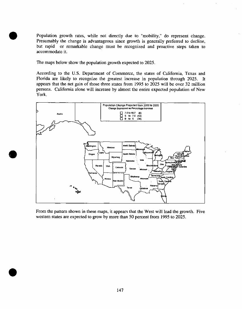
Population growth rates, while not directly due to "mobility," do represent change. Presumably the change is advantageous since growth is generally preferred to decline, but rapid or remarkable change must be recognized and proactive steps taken to accommodate it.

The maps below show the population growth expected to 2025.


t ~ a s k a l Population Change Projected from 2000 to 2005 Change Expressed es Percentage Increase

0 7.5to10.7 (6) [ ] 5 to 7.5 (12) [ ] o to s (3,=)

~ k - 4 - - - - - ~ ~ -

" " I l l i r~ i t


147

~aska

Population Change Projected from 2000 to 2015 Exloress~ in Percentage Increase

[ ] 15 to27.3 (15) [ ] 7.5to15 (21) [ ] 0 to 7.5 (16)

Montana tre

,@

South Central states will grow at a relatively fast pace. By the year 2025, shown in the map below, Texas will have recognized an 35 percent increase in total population, compared to the year 2000. This will be the highest percentage of growth in the region. Colorado will see an increase of about 24 percent followed by Oklahoma that will recognize an increase of 20 percent. The smallest gain in the region and one of the smallest in the Nation, will be in Iowa with an increase of.4.8 percent.

Population Change Projected from 2000 to 2025 Expressed in PeTcentage tncrease

[ ] 15 to 51.6 (29) [7 ?.Sto 15 (17) [ ] 0 to r.5 (6)

~e

148

Poverty


As a region, the South Central has a high percentage of children living in low income households. The U.S. percentage was 42.2 while the South Central Region had 45.4 percent of its children living in homes at that income level. Four states in the region have 50 percent or more of their children living at or below the "low income" level. Arkansas and Mississippi had the most children in low income homes with over 54 percent, followed by Louisiana and Texas.

°g a.j~


I-] 43.8to60.2 (17) [ ] 36.1to43.8 (17) I-] 0 to36.1 (18)

JL' ="

The other measure suggested here as a proxy for economic deprivation, is the Gini Index. The most recent year for which data are available by state is 1989. Each year the U.S. Department of Commerce samples persons throughout the nation to arrive at a U.S. Gini Index but the sample size is insufficient to estimate state indexes any years except full census years. While all of the Gulf coast states in the region scored high on the Gini Scale, Louisiana and Mississippi scored the highest. The Gini Index seeks to measure the disparity between the wealthiest and the poorest. The higher the index score, the greater the disparity between the wealthiest and the poorest in a jurisdiction.

149


17 0.439to0A~ 07) I'-I 0.42 to 0.4~ 07) [ ] o too.42 00)

~ a

T ~


Within the region, voting rates in the 1996 election were lowest in Texas and Arkansas, suggesting less community cohesion.

Conclusions appropriate to the South Central Region:

Louisiana has experienced a violent crime problem that is significant and likely to continue. This violent crime problem includes high rates of murder and aggravated assault in the New Orleans area but also in the rural areas of the state.

The St. Louis area has significant juvenile murder and aggravated assault problems.

Oklahoma and Central Alabama have high rates of violence, with Oklahoma's violent crime problems almost certainly associated with drug use.

Ethnic diversity and astounding growth in Texas in terms of total population and juvenile population, as well as racial diversity and poverty in other South Central states, particularly Arkansas and Louisiana, will contribute to social disorganization and increase the likelihood of higher levels of crime or disorder in the future.

150

Crime Trends and Patterns West Region

ok,.

The West Region of the United States, as defined by BJA, consists of the following jurisdictions:

Alaska Montana American Samoa Nevada Arizona New Mexico California Northern Marianas Guam Oregon Hawaii Utah Idaho Washington

The U.S. Census Bureau estimates the current population of the jurisdictions comprising the region to total 56,995,000 persons. The average of the median income for each of the states in the region for 1998 was $39,267.82, according to the Census Bureau, Housing and Household Economic Statistics Division. The average median income, by state, for 1996 through 1998 ranged from a low of $29,386 in New Mexico to a high of $51,421 in Alaska. The median income average for the United States for the period was $37,779.

The total land mass for the fourteen jurisdictions in the West Region is 1,551,125 square miles. The population density for this region is 36.7 persons per square mile. This land mass and population density is influenced significantly by the state of Alaska, which has a total land mass greater than that of the entire Northeast and Southeast Regions of the nation, combined, but with a population of only about 603,000 persons.

151

Information on crime, economy, and demographics on the territories of Guam, American Samoa, and the Northern Marianas is limited. Even the International Data Base, maintained by the Census Bureau has limited information on these territories. For these reasons, the crime data and assessment provided in the sections below include only the eleven states in the region. Summary information in the conclusion is offered regarding the territories.

Index Crime Rates in the West Region 9

The crime rate trends for index violent crimes in the West Region compare favorably with the U.S. averages. "Index crimes" reported are defined by the Federal Bureau of Investigation, Uniform Crime Reporting Program (UCR, 1998: 5):



Murder

M u r d e r R a t e s 1 9 9 1 - 9 8

J L ~

8

6

4

2

0

-[ U S

- - W e s t R e , i o n

U C R Data . Ra tes pe r 1 OO,OOO popu la t i on


152

Murder and nonnegligent manslaughter represents the most serious but rarest of crimes in the crime index. As the chart above shows, the West Region has had a slightly higher rate of murder than the average for the U.S. Beginning in 1997, however, the murder rate for the West Region fell below the U.S. average. The average murder rate for the Nation in 1998 was 6.3 per 100,000 population while the average murder rate for the eleven states comprising the West Region was 6.2 per 100,000 population. The national average murder rate was the lowest recorded since 1967.

Some of the states within the region had exceptionally low murder rates, according to an analysis of UCR .data. Hawaii had an extraordinary murder rate of 2.0 per 100,000 population, less than one-third the U.S. average. Similarly, Idaho and Utah had murder rates at about 3 per 100,000 population, one-half the U.S. average. Other states with murder rates below the U.S. average in 1998 were Oregon, Washington, and Montana. Arizona, Nevada, and New Mexico had murder rates much higher than the U.S. average.

As with most social issues, murder rates were not equally distributed in or among the states. Rural counties in New Mexico had extraordinarily high rates of murder, averaging 24.5 per 100,000 population for the 309,514 persons residing in rural counties of the state. Additionally, metropolitan areas of Nevada had the highest murder rate in the region for similar areas, with a rate of 10.2 per 100,000 population. Among the counties with population exceeding 100,000, Bernalillo County, San Juan County, and Dona Ana County New Mexico, and Clark County Nevada had the highest murder rates, each with at least 10.78 murders per 100,000 population in 1998. Notable also was Los Angeles County with 10.36 murders per 100,000 population or a total of 959 murders in 1998.

West Region Murder Rates by County 1998 Rate~ per 100,000 population

[ ] 6.:3 to 42.6 (79) [ ] t3 to 6.3 (87) [ ] 0 to 1.3 (189)

Waehlngeor Montana

Califomi

New Mexico

'= "%~l~Hawai I Arizona

153

Only about 10 percent of the 360 counties or boroughs in the Region failed to report crimes to the UCR in 1998. Twelve of these were in Alaska and 20 were in Montana. The result is a generally representative set of counties in the data set.

Eighty of the 324 counties in the region had murder rates higher than the U.S. average in 1998. Almost half of the top 25 counties in murder rates was in New Mexico.

Juvenile violence is a particularly troubling issue for many jurisdictions. Within the West Region, however, it appears that juvenile arrests for homicide are highest in only a few jurisdictions. McKinley County New Mexico had an astounding juvenile murder rate of 55 per 100,000 population in 1998. It is a county of almost 68,000 persons and there were 38 juveniles arrested for murder in 1998. In 1997, however, there were no juveniles arrested for murder in that county. This certainly suggests that 1998 was an aberration, unless high rates continue.

West Region Juvenile Arrest Rates for Murder 1998 Arrest rates per 1GO,000 total population

1"7 1.5 to 56 (37) 0.33 to 1.5 (30) 0 to 0.33 (288)

W a s h i n g t o n ~ Montana O r e g ° n ~ h o

C a l i f o m i ~ = ~ N e w Mexico

~Hawaii Arizona

Care should be exercised in interpreting rates for one year, particularly in sparsely populated areas. Single year anomalies do not suggest a pattern and serve simply as a warning that patterns might develop. Chaves County New Mexico, Twin Falls County Idaho, and Tooele County Utah also had high rates of juvenile arrests for murder in 1998 but in order to determine a pattern of problems, prior years must be assessed.

The West Region counties in the national map appear to have more "hot spots" regarding murder rates, per 100,000 population. One explanation for that appearance is the geographic size of counties in the West Region, compared to the other regions. Large counties appear more prominent in these shaded maps.

154

U S Murder Rates b y ~ " R=es Pe~ 100'000 P°Ot'a~i°n I I

[3 s.3to 134 mso) I I Ii] 1.3to 8.3 m47~ I1 0 o to 13 o849~___J

It does appear from the data, however, that New Mexico, Arizona, Nevada and significant portions of California had higher than average murder rates in 1998..

I ' i¢~t,o , ' s o ~ t h I)ad~==

Two states, New Mexico and Nevada, had murder rates higher than 9.7 per 100,000 in 1998. Most states were in the lower range, however. The chart below shows the

regression line, based on past rates.

155

Regional Projected Murder Rates Murder Rates West Region 1991-98


~o4

oJ

e4

74

04

m

o O b s e r v e d

~ ' o Linear

o Projected

G O

/

The trend lines projected and observed are qui te consistent and the projected line would suggest that the murder rate in the region will increase slightly in 1999 then continue to decrease in future years.

As stated earlier, murder is the most serious of crimes reported to police, and it is the one most likely to be reported when it occurs. The reliability and validity of the statistic makes it one of the best measures of violence, based on official statistics (there are more valid methods of measuring other crimes than official statistics). Since it is a relatively rare event, it becomes difficult to determine patterns or trends in areas with low populations since a few crimes can cause unusual spikes in rates. It appears, based on historical information, that murder is a significant problem in two states in the West. New Mexico, particularly Bernalillo County and rural areas of the state, as well as Clark County Nevada, have serious murder problems. Guam's murder rate in 1998 was 6 per 100,000 population, suggesting consistency with the national rate.

Rape

Just as murder is one of the crimes most likely to be reported when it occurs, rape is one of the most underreported crimes. Since there is a gap between the actual number of forcible rapes occurring (or attempted) and those reported to police as having occurred or attempted, it is sometimes difficult to determine whether high rape rates mean more rapes occur or more rapes are being reported. The crime is certainly a serious one and regardless of the interpretation, the data should be studied and the degree of the problem assessed. Later there will be recommendations on how best to judge the trend or pattern of rapes reported to police.

156

As was true of murder, the West Region has rape rates that have been higher than the U.S. average. As the chart below shows, the states of the West Region had forcible rape rates that came into consistency with the U.S. rates in 1997 and remained consistent with the National rates in 1998.

Rape Rates 1991-98

50

45

40

35

30

25

20

15

10

m _ . . %

- - U S

- - W e s t Region


In 1998, the U.S. average for forcible rape rates was 34.4 per 100,000 population while the average for the region was 34.6 per 100,000 population. There have been no unusual spikes or valleys in the trend line for the region and the rates have decreased faster than the slope shown in the national rates.

When unusual spikes appear in the rates of sexual assaults reported to police, over time, for a jurisdiction such as a state, it may suggest an extraordinary increase in sexual assaults or, arguably, it may suggest an aggressive and effective effort to facilitate reporting of the crime when it occurs. Victim Assistance Coordinators, Rape Crisis Centers, and persons within prosecutor offices may be effective in reducing the gap between the number of crimes occurring and the number of crimes reported. On a regional basis, it appears that there are no unusual patterns in the data so the supposition is that the data reflect the same rate of reporting, year after year. Utah's rape rates, for example, showed unusual increases in 1990 and 1991. Investigation by Utah's Commission on Criminal and Juvenile Justice showed rather conclusively that the

157

increases were due to new Victim Assistance Units improving the reporting of crimes rather than a significant increase in the occurrence of crimes.

State-level rape rates show that Alaska had an extremely high rape rate of 68.6 per 100,000 population for 1998, a rate higher than any other state in the region. That rate was also the highest in the nation. As was stated earlier, 12 jurisdictions in Alaska did not report to the UCR Program. This is why some of the jurisdictions do not reflect high rates in the map below. Based solely on those jurisdictions that did report however, there were so many rapes that if the non-reporting jurisdictions had no crimes, the rate for Alaska would still exceed 61 per 100,000 population for the entire population of the state.

West Region Rape Rates by County 1998 Rates per 100,000 iooptd~ion

39 to246 (101) B 21.9to 39 (94) [] 0 to 21.9 (160)

W a s h i n g t o n ~ Montana

Oregon~h o ~ Utah

C a l i f o m i a ~ ~ . l ~

" ~lb - ' ~ N e w ~ " - r - x r l ,~v",r-c-J-~JI Meldco

~Hawali

This map shows that there are pockets of higher than average rape rates within the West Region. New Mexico, Nevada, and portions of Washington had high rape rates.


As the U.S. map below shows, there are pockets of high forcible rape rates throughout the Nation, including the West Region. Again, this map excludes many Montana Counties and Alaska jurisdictions since those data were not available.

158

;z ~'

, . ~ ~ .~,,- . . . . - . . . ,<,::~,,,;. ,

U.S. Rape Rates by' County 1998 Rates per 100,00010optd~on

[ ] 39 to 986 (650) [ ] 21.9to 39 (651) [ ] 0 to 21.9 (1S42)

I~ql~kZ= U .~ V I ~ I~la=ds

On a state-wide examination, the West Region appears to have high forcible rape rates, compared to other states. As the map below shows, the rates were highest in Alaska, New Mexico, and Nevada but also high in Washington, Oregon and Utah.

Rape Rate 1998 R~tes per 100,000 populatio~

17 4stoss.6 CO [ ] 3Sto49 (13) [ ] oto 3s (3~

I ~ ' I M o n l I r t a - - ' Nolt~ I ] = k ° t a l "1

Specifically, the rape rates for the highest states were: Alaska 68.60 Nevada 52.10

159

New Mexico 55.10 Oregon 39.80 Utah 41.70 Washington 48.20

It should be noted that New Mexico and Nevada also had very high murder rates in 1998.

As was the case with murder, the trend line for rape in the West Region is strongly declining.

Regkmal Projected Rape ?_ates Rape Rates West Region 1991-98

Observed and Projected 50~

~4

30~

201

" Observed

o Linear

o Projected 00 01 02 03 9 4 95 00 97 9:8 99


Robbery


As the chart below shows, the West Region has experienced higher than average robbery rates although the gap narrowed in 1997 and the rate is now consistent with that of the U.S. The U.S. robbery rate in 1998 was 165 per 100,000 population. The rate was significantly higher, 198 per 100,000 population, for metropolitan areas of the Nation.

160

The robbery rate in the West Region in 1998 was 174.5 per 100,000 population. While this may appear to be a laudatory trend, it is imperative to remember that the population density is low and there is a dearth of metropolitan areas in many states of the region. One would expect the robbery rate to be lower, given the non-urban nature of many of the jurisdictions.

Robbery Rates 1991-98

3OO

200

150

100

50

| I I ! !

~ U S

~ V~est ][legion


Even though the West has had robbery rates higher than the U.S. average, the rate of decline has been steeper and the highest rates have been restricted to very few jurisdictions.


161

West Region Robbery Rates by County 1998 J - - % Rates per 100,000 poput~ion

~--~------~-,- ~ [ ] 62.8 to 3,230 C72)

'~=¢~" W a s h i n g t o n ~ Montana

O r e g o n ~ h o

~ Utah C a l i f o m i ~

• " ~ [ ~ 1 ~ New Mexico

~lbHawaii

Those counties along the West coast and within the most densely populated areas of the region had the highest rates of robbery. It should be noted that the ranges for this map and the robbery maps for other regions use relatively low rates, even for the highest range. This is done to show where, within each region, the rates are highest and may be useful in assessing drug-related offenses as well. Robbery is one of the crimes frequently associated with drugs and, while it cannot serve as a proxy for drug use, may help to focus attention on a serious violent crime which may also serve to reduce drug-related offenses.

The ten counties with the highest robbery rates in the region in population greater than 500,000 persons. rates:

San Francisco California Bernalillo New Mexico Clark Nevada Los Angeles California Alameda California Multnomah Oregon Sacramento Califomia San Joaquin California Fresno California Pima Arizona

1998 each had a

These were, in order from highest robbery

The range of robbery rates shown by these jurisdictions was 533 per 100,000 population for San Francisco County to 218 per 100,000 for Pima County.

Nationally, the West Region reflects more "hot spots" than was seen in previous crime maps, as is evident in the map below.

162

. , . ° . ~ . U.S. Robbery Rates by County 1998

R~tes pe r 100 ,00~ pepu l~ i on

[ ] 62.8 to 3,230 (651) [ ] 20.91o 62.8 (652) [ ] 0 to 2o90s40)

The U.S. map depicting the rates for robbery by state show New York and Maryland as being among those states with the highest robbery rates. According to UCR analysis of robbery rates, the Western States (the FBI does not use the same group of states to form the West Region as does BJA so exact comparisons are not possible) have far higher incidents of commercial robberies and bank robberies than other regions of the nation.

Clearly, robbery rates were highest in Nevada (254 per 100,000) and California (210 per 100,000), as shown below.

163

. Jillsl<;i L

Robbery Rate 1998 R~ie~l per 1(]0,000 populalion

[ ] lgOtoSSO (9) [ ] 140tolg0 (11) [ ] 0 to 140 (32)

t t L " ~ i<-,ol---_-;_, o" -

Again, the robbery rate trend line, as reflected by the regression line, is strongly downward. Based on this projection, the robbery rates in the West Region of BJA are likely to be at or below the U.S. averages by 1999 or 2000.

Regional Projected Rq)bbc ry Rates

Robbery Rates West Region 1991-98


2ool

lOOl

n

*.ll Obiewed

o Lineal

o Plojected

164

Aggravated Assault

Aggravated Assault, an assault often accompanied by the use of a weapon, is the most frequently occurring of the serious violent crimes. The U.S. average for aggravated assault in 1998 was 360.5 per 100,000 population. While the average for the West Region was higher than the national average in 1998, only four states within the region had rates that were higher than the U.S. average in 1998.

As the table below shows, the West Region has had and continues to have higher than average aggravated assault rates. This is due, in part, to the extraordinarily high rate in New Mexico.


6 0 0

. ~ ~ l ' ~ ~ ~ m ' i ~ ~

2 0 0

1 0 0

0 '1 I I I

~ U S West Region


Clearly, the distribution of aggravated assault rates varies significantly. As the map below shows, there are pockets of violent, serious assaults within the region.

165

West Region Aggravated Assault Rates by County t 998 Rales per 100,000 population

[ ] 345.9to 13,000 (95) [ ] 180.2to 345.9 (93) [ ] 0 to 1B02 (16"/)

W a s h i n g t o n ~ Montana

O r e g ° n ~ l d a h o

~ New Mexico

" I=~ Arizona ~lbHawal I

The obvious pockets of violence are those jurisdictions in New Mexico, California, and Alaska, as well as some pockets in Arizona.

% • . , , e . . ,

US Aggravated Assault Rates by County 1998 Rates per 100,0130 population

[ ] 34S~to 13/~0 (6S0) t--I lS02to 34s.s (65o) [ ] o to 18o.2 (1843)

The national county-level map above shows that the pockets and clusters of high aggravated assault jurisdictions in the West are as striking as those in the Southeast.

166

jo t =

Aggravated Assaul t Rate 1998 Rstes per 1(~0,000 pop,.d~ion

[ ] 495 to 944 (8) [ 7 350 to 495 (11) t - t o to~so (33)

~eT-~--~. ~ -~ ( ' M. - r ~ i~,,. ~,or, tana ~ _._.. L _ t " " ' ¢ ~ " ~ - ' - ' ~ / I

' "~, N h o m a Te~'~L~ $ e 'J

v

The state-level map above shows clearly that New Mexico is the state with the highest aggravated assault rates in the region. New Mexico also had extremely high murder rates, rape rates, and burglary rates in 1998

Again, the rates are declining in the West and the Nation although the rates in the West may not decline in 1999.


Aggrevated Assaufl Rates West Region 1991-91


90 0t 02 ~3 04 ~ ~ 07 08

167

This projection of the regression line shows the decline of aggravated assault in the West Region and suggests that the decline will continue after a flat year in 1999. The states and counties representing pockets of violence, however, should not be masked by this trend.

Drug Use in the West Region

One of the issues of importance to the Bureau of Justice Assistance and the states is the use of illegal drugs. Assessing the use of drugs is even more problematic than assessing the incidence of crime. Drug arrests have, historically, been one of the major indices of drug presence in a jurisdiction, even though estimates are used widely (See Methodology). Drug interdiction and drug arrests are, however, clearly tied to resources and policy decisions. Drug enforcement is proactive enforcement. If a jurisdiction has resources, human and otherwise, to focus on drug arrests, arrests occur thus proving the presence of drugs. If a jurisdiction lacks sufficient resources to proactively address drug possession and drug sales, the lack of arrests might spuriously suggest the absence of illegal substances. Similarly, policy decisions often determine the location of proactive drug enforcement, ff drug arrests occur in a neighborhood, community, or school, it certainly means there were drugs present in those locations. If, however, no proactive enforcement occurs in a neighborhood, community, or school and no drug arrests are made, it does not necessarily mean that there were no drugs present.


As the map below shows, drug arrests in the region are concentrated in California, Nevada, and Arizona. California had the highest rate of drug arrests in the region, with 809 per 100,000 population, followed by Arizona with 641 per 100,000 population and Nevada with 624 per 100,000 population.

168

West Region Drug Arrest Rates by County 1 998 Arre~st redes per 100,000 populalion

[] 5013.9 to 3,S50 (134) [ ] 301.3to 506.9 (96)

i l ~ ~ 0 to 3013 (12o")

W a s h i n g l o n ~ Montana

O r e g ° n ~ d a h o

~ Utah

C a l i f ° m i ~ N e w Mexico

~l'Hawaii


west Region Drug Possession Arrest Rates by County 1 gg8 Arrest r~es loaf I00,000 p o l ~

i'-I 39;,.sto3,s.so (1,=s) 225,6to 397.6 (86)

o to 22sJs (124)

% W a s h i n g t e n ~ Montana

O r e g ° n ~ d a h o

~ Utah

: ~ N e w Mexico "%

~-Iawaii Arizona


169

As the map below shows, the pattern of arrests for drug sales and manufacture, while generally consistent with possession shows some differences for Nevada.

West Region Drug Sales Arrest Rates by County 1998 .__/,'- - - ~ - - - - - ~ A . = ~ ,=es ~ loo,ooo pop,,t~o.

=~¢=;~ * W a s h i n g t o n ~ Montana

Oregon~h o ~ Utah

C a l l f o m i ~

1 ~ ~ [ ~ New Mexico "%

(~Hawall Arizona

As the map rather clearly shows, Nevada is far less involved in arrests for drug sales, compared to drug possession. The same is true of Oregon. This observation is not intended to be a critique. Many issues fit into the decisions to engage in certain types of proactive enforcement.


170

TEDS 1997 Drug Treatment Rates Rate~ per 100,000 too l~on

[ ] 100totSt (9) I--] 50to100 (22) [ ] Oto 50 (21)




The highest rates for drug treatment in 1997 in the West Region, the most recent year for which data were readily available, were observed in Washington and Oregon. These data are somewhat inconsistent with the arrest data. It should be noted that Arizona did not participate in the TEDS program in 1997.

171

TEDS 1997 Heroin Treatment Rates Rates pet 100,000

[ ] 40 to109 (8) [ ] 7.5to 40 (10) [ ] 0 to 7.s (34)

-,a i The map above shows the rates of treatment for heroin use, according to TEDS for 1997. The West Region is the major cluster of the nation regarding heroin treatment. Within the region, treatment rates were highest in California (47.5 per 10,000) and Oregon (42.4 per 100,000) for heroin use. While these states were highest in the region, the rates of heroin use were not as high as those in the Northeast.

Below, we see the states with the highest rates of treatment for cocaine and crack cocaine. The treatment data suggest that cocaine is not a significant problem in the West Region.

172

r ~" Abel=

• " ¢=%,

"rEDS 1997 Cocaine Treatment Rates Rates per 100,000 POl0taalion

17 3 .5 to57.6 (7) [ ] 18to 35 (16) [ ] 0 to 18 (29)

(/ t! i " " " I) ii ~ l - - ~ - - t - 4 "-"

'~ ~ A .= ,n~-T- - "V"- -~ - " ' ~ -.7. -e

There is clear evidence that stimulant use in 1997 was highest in the West Region of the Nation. It appeared not to represent a problem for the rest of the Nation but is a significant problem in the West. Most of this use was methamphetamine. Oregon had the highest rate of treatment for stimulants, followed by Nevada, California, and Montana.

TEDS 1997 Stimulant Treatment Rates Rates per 100,000 popuZ~

[ ] lS to55.4 (10) I - I l ~ t o l s (12) [ ] o to 1.s (3o)

173

It is suggested that TEDS represents a viable corollary to arrest data in understanding the presence of drugs within certain jurisdictions. These data help to better understand drug use as well as enforcement strategies.

Social and Demographic Issues in the West Region ~°







~o See "Methodology" section at the end of the document for social and demographic data sources, limitations and methods used in this assessment.

174


Heterogeneity, Growth and Change in the West Region



Ethnic Diversity 2025

[ ] 0.34to o.s (7) [ ] 0.22to0.34 (6) [ ] 0 to022 (39)

Ethnic diversity is based on the formula (1 - ~,p°) where p is the proportion of the population in each of the categories of Hispanic and Non Hispanic. Racial diversity,

175

described below, is based on the same formula but where p represents the proportion of persons in each of the racial categories. These formulas were used by Warner and Pierce (1993) in applying social disorganization theory to crime data.

Ethnic diversity, shown in the map above, is likely to be greatest in the West. It is projected by the Census Bureau that by 2025, Hispanics will represent 48 percent of the population of New Mexico, 43 percent of the population of California, and 32 percent of the population of Arizona.

Racial diversity, shown in the map below, will affect much of the Nation, including the West Region states. By the year 2025, it is expected that the Asian and Pacific Islands racial category will represent about 18.4 percent of the population of California and 22 percent of the population of Alaska. Hawaii will have 66 percent of its population Asian and Pacific Islander. It is projected that by 2025 one-third of the citizens of Maryland will be black and more than 20 percent of the citizens of New York will be black.

Racial Diversity Scores 2025

I-I 0.34 to 0.54 (17) [ ] 0.22to0.34 (17) [ ] 0 to0.22 (18)

h Idah°' : ~ ~e s

~ f

P ~ o ~

The combinations of racial diversity and ethnic diversity will have greatest effect on California within the West Region. It is imperative that, among other things, states insure that their criminal justice agencies and other governmental agencies reflect the diversity of the population.

In the next of map, the change in the juvenile population is described. The Census Bureau projects that the nation's youth will account for a smaller proportion of the population in 2025 than in 1995. Within the West Region, California is expected to see a growth of 70 percent in the number of persons aged 5 through 17 by the year 2025, the largest growth in the Nation. This growth rate will be greatest from 2015 through 2025. Hawaii will see an increase in juvenile through 2005 then another growth period from

176

2015 to 2025. The percent growth in juveniles in Hawaii will be 60 percent. Alaska and New Mexico will see 42 percent growth in their juvenile population, generally from2005 to 2025. Montana will recognize the slowest growth in juveniles in the region, with only a 2 percent increase.

, . " - Percent Change in Juvenile Population 1995-2025

[ ] is to 7o., c~ [ ] 0 to15 (21) [ ] - l r ~ t o 0 (14)

Mobility in the West Region

Mobility is represented by data collected by the Census Bureau on domestic migration (migration from state to state) and international migration (migration from other countries). Six states in the region have experienced increases in domestic migration in the past decade. Nevada has experienced the greatest increase, 24 percent, in the nation while Arizona (12.1 percent), Idaho (10.9 percent) and Oregon (8.2 percent) have also seen net increases due to domestic migration. California and Hawaii have recognized net losses of 6.6 percent and 8.4 percent respectively..

177

")j4y

Changes in Population due to Domestic Migration 1990-g9 Char~=s Expe¢~ ~ Perce~t=~es

[ ] 5.2 to 24 (11)

El -283to -05 (20)

'WCi[ .......

The map below shows that international migration has benefited California (6.9 percent increase in population), Hawaii (4.2 percent increase) and Nevada (3.1 percent increase).. California recognized the highest gain in the nation.

" fZ"

~ m : D

Population Change 1990-99 due to International Migration O~r~e Expressed =s ~

[ ] 2 t o s ~ (17) [ ] 0.74 to 2 (17) [ ] 0 to0.74 (lS)


178


The maps below show the population growth expected to 2025.

According to the U.S. Department of Commerce, the states of California, Texas and Florida are likely to recognize the greatest increase in population through 2025. It appears that the net gain ofthose three states from 1995 to 2025 will be over 32 million persons. California alone will increase by almost the entire expected population of New York.

Population Change Projected from 2000 to 2005 Change Exlxessed as Perc~aage Increase

[ ] 7.5to10.7 (6) [ ] 5 to 7.5 (12) [ ] 0 to S (34)

From the pattern shown in these maps, it appears that the West will lead the growth. Five western states are expected to grow by more than 50 percent from 1995 to 2025. The growth will begin with Nevada, Idaho, Utah, Arizona, and New Mexico. California, New Mexico, Hawaii, and Utah grow fastest during the period 2000 to 2015.

179

PopulaUon Change Projected from 2000 to 2015 Change Expensed in Percentage Increase

[ ] 15 to27.3 (15) [ ] 7.5to15 (21) I-I o to 7.s (IS)

II \

West states will grow but at a far slower pace. By the year 2025, shown in the map below, California will have recognized a 51.6 percent increase, the greatest in the nation. California is expected to add 2 million persons from 2000 to 2005, 7 million from 2005 to 2015, and 8 million from 2015 to 2025. the eight states with the highest percentage increases in population through 2025 are California, New Mexico, Hawaii, Arizona, Nevada, Idaho, Utah, and Alaska. Clearly, the West Region should brace itself for unprecedented and unparalleled growth.

~'~ r PopulaQon Change Projected from 2000 to 2025

Change Expressed in Percer~ege In.ease

[ ] 15 to51.6 (29) [ ] 7.5to 15 (17) [ ] 0 to 7.5 (6)

_ ~ F - - - - q N /

!

180

Poverty


As a region, the West has had a high percentage of its children living in low income households. The U.S. percentage was 42.2 while the West Region had 45.5 percent of its children living in homes at that income level. New Mexico had the highest percentage in the region and second in the Nation (the District of Columbia was highest), at 57 percent. Alaska and Utah had very low percentages of children living in low income households.

Average Percent of Chllclren in Poverty, 1996-98

[ ] 43.8to60.2 (17) [ ] 36.1to43.8 (17) [ ] o to3s.1 (18)

..,,5 /~ . - ' '~ "- '~-- - - . . .~ . . . ,~ .~

, a

The other measure suggested here as a proxy for economic deprivation, is the Gini Index. The most recent year for which data are available by state is 1989. Each year the U.S. Department of Commerce samples persons throughout the nation to arrive at a U.S. Gini Index but the sample size is insufficient to estimate state indexes any years except full census years. California and New Mexico had the highest rates in the region. The Gini Index seeks to measure the disparity between the wealthiest and the poorest. The higher the index score, the greater the disparity between the wealthiest and the poorest in a jurisdiction.

181


[ ] 0.43~ to 0A92 (17) [ ] 0A2 to 0.439 (17) I-1 0 to0.42 (18)

~*~ "~" ~i t~n it------ I


Within the region, voting rates in the 1996 election were lowest in Hawaii, Nevada, and Arizona.

Conclusions appropriate to the West Region:

Violent Crime has been and is likely to continue to be highest in New Mexico, particularly rural areas of the state and Albuquerque; metro areas of Nevada, particularly Clark County; Alaska, with a strong influence from alcohol use among juveniles; certain urban areas of California; and Multnomah, Oregon.

In the next 25 years, due to growth and diversity, pressure will be placed on the justice system as an effective means of social control in Nevada, California, New Mexico, Alaska, and Hawaii.

Juvenile crime will be a significant factor in California, especially 2015-2025; Alaska and New Mexico, especially beginning in 2005; and Hawaii, throughout the next 25 years.

As juvenile-preferred drugs develop, especially in Western states, all drug use and abuse will have greater impact and influence on crime, including violent crime and property crime.

182

New Mexico is likely to remain a major pocket of violent crime but Califomia's growth is likely to produce increases in crime, including violent crime. The two state's change patterns, low income levels, heterogeneity, and historical crime patterns suggest ominous crime and drug trends for the future.

High rape rates in Alaska and high violent crime rates in New Mexico and Nevada, combined with drug abuse problems in Oregon, and dramatic growth in juveniles and Hispanic populations in California, suggest that the West Region is likely to be an area of concern in the future.

183

Methodology

The approach used in developing the charts, graphs, maps, and assessments is one that has been used in numerous jurisdictions at the state and local levels. This was the first time it has been used at the regional level and, given the lack of homogeneity of the jurisdictions in some of the regions, this may not be as useful as state-specific assessments. Regional assessment, however, was requested.

The first step in conducting the assessment was to gather crime and arrest data. These data came from several sources but all emanated from the Federal Bureau of Investigation's Uniform Crime Reporting Program. The eight-year charts showing each region's violent crime rates compared to the United States' crime rates were based on data from each year's UCR Table 4. Similarly, the 1998 U.S. maps of crime by state were based on Table 4. As such, the UCR notes:

Because not all law enforcement agencies provide data for complete reporting periods, estimated crime counts are included in these presentations . . . . . Using the known crime experiences of similar areas within a state, the estimates are computed by assigning the same proportional crime volumes to nonreporting agencies. The size of the agency; type of jurisdiction, e.g., police versus sheriffs office; and geographic location are considered in the estimation process.

Each year's UCR includes the notes on states which do not report complete or sufficient data and for which estimation is necessary.

The county-level data were derived from UCR data tapes, extracted from data maintained by the Inter-University Consortium for Political and Social Research. These data include county-level information on crimes reported and arrests. The following is an excerpt from the 1998 codebook for these data:

(1) Two major changes to the Uniform Crime Reports (UCR) county-level files were implemented beginning with the 1994 data. A new imputation algorithm to adjust for incomplete reporting by individual law enforcement jurisdictions was adopted. Within each county, data from agencies reporting 3 to 11 months of information were weighted to yield 12-month equivalents. Data for agencies reporting less than 3 months of data were replaced with data estimated by rates calculated from agencies reporting 12 months of data located in the agency's geographic stratum within its state. Secondly, a new Coverage Indicator was created to provide users with a diagnostic measure of aggregated data quality in a particular county. Data from agencies reporting only statewide figures were allocated to the counties in the state in proportion to each county's share of the state population.

(2) In the arrest files (Parts 1-3 and 5-7), data were estimated for agencies reporting 0 months based on the procedures mentioned above. However, due to the structure of the data received from the FBI, estimations could not be produced for agencies reporting 0 months in the Crimes Reported files (Parts 4 and 8). Offense data for agencies reporting 1 or 2 months are estimated using the above procedures. Users are encouraged to refer to the codebook for more information.

185

(3) No arrest data were provided for Florida, Kansas, Wisconsin, and Washington, DC. Limited arrest data were available for Illinois, Kentucky, and New Hampshire. Limited offense data were available for Alaska, Illinois, Kansas, Kentucky, Mississippi, Missouri, Montana, South Dakota, and Wisconsin.

(4) UCR program staff at the Federal Bureau of Investigation (FBI) were consulted in developing the new adjustment procedures. However, these UCR county-level files are not official FBI UCR releases and are being provided for research purposes only. Users with questions regarding these UCR county- level data files can contact the National Archive of Criminal Justice Data at ICPSR.

The appropriate citation for these data is: U.S. Dept. of Justice, Federal Bureau of Investigation. UNIFORM CRIME REPORTING PROGRAM DATA [UNITED STATES]: COUNTY-LEVEL DETAILED ARREST AND OFFENSE DATA, 1998 [Computer file]. ICPSR ed. Ann Arbor, MI: Inter-university Consortium for Political and Social Research [producer and distributor], 2000.

Next the data, state-level and county-level, were geocoded for mapping purposes. All 3,145 counties or county-like jurisdictions in the nation were similarly linked to the data for that particular location. Rates were established based on population statistics in the crime and arrest data, consistent with estimates from the U.S. Census Bureau.

The limitations on the use of UCR data are evident. Nonreporting jurisdictions will have rates estimated and imputed. While these rates are the best estimates available, they are, nonetheless, estimates. The options are: (1) use the estimates as the best evidence available of crime in a jurisdiction; (2) reject the data and calculate no information on something as important as crime within a jurisdiction; or (3) supplement the estimated data with information from other sources such as victimization surveys. For purposes of this project, option 1 was selected. For better information and insight, option 3 is the clear choice. Survey data were not available for all jurisdictions so, for the Summer 2000 conferences, it would have been inappropriate to report crime from only a few jurisdictions. Option 2 is the least responsible choice. In the absence of better data, UCR data remains the best, most reliable information available.

Drug arrest data were suspect, based on nonreporting as well as the data's reflection of policy decisions as much as or more than the actual use of drugs. Other drug use data were sought and the Treatment Episode Data Set was utilized. The citation for this dataset is:

U.S. Dept. of Health and Human Services, Substance Abuse and Mental Health Services Administration, Office of Applied Studies. TREATMENT EPISODE DATA SET (TEDS), 1997 [Computer file]. 2nd ICPSR version. Chicago, IL: National Opinion Research Center [producer], 1999. Ann Arbor, MI: Inter- university Consortium for Political and Social Research [distributor], 1999.

186

These data included more than 396,000 cases or episodes of treatment. The following comments are excerpted from the TEDS (1997) codebook:

Universe The universe for TEDS is treatment admissions to substance abuse treatment units receiving federal funds. Treatment units receiving any federal funds are requested to provide TEDS data on publicly and privately funded clients. There are some instances, however, in which information is provided only for clients whose treatment is funded through public monies. Response rates TEDS attempts to include ("capture") all admissions to providers receiving any public funds. Because each state or jurisdiction decides the TEDS eligibility of a provider, there is no independent check on the actual sources of funding. For 1997, the estimated inclusion rate for TEDS-eligible providers was 85 percent, with the inclusion rate for all treatment providers estimated at 58 percent (including privately funded providers). A more complete discussion is provided in Appendix B of Treatment Episode Data Set (TEDS), 1992-1997: National Admissions to Substance Abuse Treatment Services". Data Limitations Some limitations regarding the use of the TEDS files should be noted. TEDS is collected by states according to their own systems for monitoring substance abuse treatment and then crosswalked to the TEDS data elements, according to a mutually-approved protocol. Given variation among the states in how they define and collect substance abuse treatment data, the following should be considered when using these data: 1. The way an admission is defined may vary from state to state such that the absolute number of admissions is not a valid measure for comparing states. 2. States continually review the quality of their data processing. As states identify systematic errors, they may revise or replace historical TEDS data files. While this system improves the data set over time, reported historical statistics may change slightly from year to year. 3. The number and client mix of TEDS records depends, to some extent, on external factors -including the availability of public funds. In states with higher funding levels, a larger percentage of the substance abusing population may be admitted to treatment, including the less severely impaired and the less economically disadvantaged. 4. Public funding constraints may direct states to selectively target special populations, for example, pregnant women or adolescents. 5. States vary in the extent to which coercion plays a role in referral to treatment. This variation derives from criminal justice practices and differing concentrations of abuser sub-populations. 6. States vary in their reporting practices. For instance, drunk drivers who are referred to education or treatment are excluded from TEDS reporting in all but a few states. 7. TEDS includes treatment admissions and in many states the files may include multiple admissions for the same client. Therefore, any statistics derived from the data will represent admissions, not clients. It is possible for clients to have

187

multiple initial admissions within a state and even within providers that have multiple treatment sites within the state. A few states uniquely identify clients at the state-level and several more states are attempting to achieve this level of client identification. The TEDS provides a good national snapshot of what is seen at admission to treatment, but is currently unable to follow individual clients through a sequence of treatment episodes. 8. The TEDS distinguishes between "transfer admissions" and "initial admissions." Transfer admissions include clients transferred for distinct services within an episode of treatment. Only initial admissions are included on the public use files.(Emphasis in original source.)

Clearly the SAMSHA, Office of Applied Statistics, staff are conscientious in their activities but there are some data limitations that cannot be resolved. These data do, however, offer better indications of the nature and extent of drug abuse than arrest data.

These data were grouped by state, rates established, and the data were geocoded for thematic mapping.

Other data were located which were believed to be instructive in assessing social and demographic issues, consistent with criminological theory. The theories relied upon were those generally consistent with social ecology or "Social Disorganization." The theory suggests that heterogeneity, mobility, and poverty or economic deprivation will be important in explaining the location of crime, violence, and disorder. Consistent with this approach, demographic data were gathered from several sources.

Economic deprivation can be measured many ways. One of the accepted and reasonably available methods is to measure the percentage of those under the age of 19 who live at or below 200 percent of the poverty level. This is not technically "children in poverty" but a measure of those who live in desperate circumstances. These data were derived from the U.S. Census Bureau. As stated in Dalaker (1999):

Following the Office of Management and Budget's (OMB's) Statistical Policy Directive 14, the U.S. Census Bureau uses a set of money income thresholds that vary by family size and composition to detect who is poor. ff a family's total income is less than that family's threshold, then that family, and every individual in it, is considered poor. The poverty thresholds do not vary geographically, but they are updated annually for inflation using the Consumer Price Index (CPI-U). The official poverty definition counts money income before taxes and does not include capital gains and noncash benefits (such as public housing, medicaid, and food stamps). Poverty is not defined for people in military barracks, institutional group quarters, or for unrelated individuals under age 15 (such as foster children). They are excluded from the poverty universe--that is, they are considered neither as "poor" nor as "nonpoor."

Specifically, the data showing the percent of children (under 19) at or below the poverty level, averaged for the three years 1996-98 were used. The standard error of the average percent ranged from 1.2 (California) to 3.7 (District of Columbia) but generally reliable. These data were the most recent available and were geocoded for mapping.

188

Another indicator of relative deprivation was the Gini Index. It is an index of income concentration. The ratio is a statistical measure of income equality ranging from 0 to 1. A measure of 1 indicates perfect inequality; i.e., one person has all the income and rest have none. A measure of 0 indicates perfect equality; i.e., all people have equal shares of income. The data and explanations can be found in "Current Population Reports, Series P-60, No. 123." U.S. Census Bureau, Population Division, Fertility & Family Statistics Branch, Maintained By Laura K. Yax (Population Division). These data were available at the state level only for 1989 although they were available nationally, through sampling, for more recent years.

Race, ethnicity, and age were gathered, by state, although they were available at the county level. The state level was viewed as sufficient for purposes of determining migration trends. State-to-State migration data were used to model migration flows between States explicitly. Similarly, race, ethnicity, age, and total population were extracted from U.S. Census Bureau data, by state. Without going into too much detail, the following excerpt captures the essence of the development of the data by the Census Bureau (Campbell, 1996):

The 1995 to 2025 State population projections were prepared using a cohort- component method. Each component of population change --- births, deaths, State-to-State migration flows, international in-migration, and international out- migration --- was projected separately for each birth cohort by sex, race, and Hispanic origin. The race/ethnic groups projected were non-Hispanic White; non- Hispanic Black; non-Hispanic American Indian; non-Hispanic Asian; Hispanic White; Hispanic Black; Hispanic American Indian; and Hispanic Asian The basic framework was the same as in past Census Bureau projections. Detailed components necessary to create the projections were obtained from vital statistics, administrative records, census data, and national projections.

The cohort-component method is based on the accounting system:

P1 = P0 + B - D + DIM - DOM + IIM - IOM where:

P1 = population at the end of the period P0 = population at the beginning of the period B = births during the period D = deaths during the period DIM = domestic in-migration during the period DOM = domestic out-migration during the period

(Both DIM and DOM are aggregations of the State-to-State migration flows)

IIM = international in-migration during the period IOM = international out-migration during the period

traditional demographic

To generate population projections with this model, we first created separate data sets for each of these components. The assumptions and procedures by which these data were generated by single year of age, sex; race, and Hispanic origin are

189

described in the following sections. In general, the assumptions concerning the future levels of fertility, mortality, and international migration are consistent with the assumptions developed for the national population projections released by the Census Bureau.

Once the data for each component were developed, it was a relatively straightforward process to apply the cohort-component method and produce the projections.

These projections were calculated based on rates of change and the data are reflected in the document. The methodology used by the Census Bureau appears to reflect every variable that can be reasonably measured in assessing rate of change. At the state level, it is expected that the data will be extremely accurate, with the accuracy deteriorating at the local levels.

Once the racial and ethnic characteristics were determined, calculated, and categorized within the datasets, heterogeneity was calculated based on the formula used by Warner and Pierce (1993). The resulting ratio scale would have allowed more complex analyses than simply describing the differences and relative position of states and jurisdictions but no further analyses were conducted due to time limitations.

One other dataset proved valuable in serving as an example of data that could be useful in determining social cohesion. These data were voting rates of registered voters within jurisdictions. These data are compiled by U.S. Census Bureau. Population data from U.S. Census Bureau, Current Population Reports, P25-1117 and Statistical Brief (SB/96-2); votes cast from Elections Research Center, Chevy Chase, MD, America Votes, biennial, (copyright); and 1994, Congressional Quarterly Inc., Congressional Quarterly Weekly Report, Vol. 53, No. 15, April 15, 1995 (copyright).

The weakest element in the methodology is the crime and arrest data, due to reporting inconsistencies. The data are used here, however, to establish "indications" of problems and then apply other data to determine the likelihood of continuation of the problems.

190

Major References Used in the Document

Anselin, Luc, Jacqueline Cohen, David Cook, Wilpen Gorr, and George Tita. (2000) "Spatial Analyses of Crime" In Measurement and Analysis of Crime and Justice, Vol. 4. Crime and Justice 2000. Washington, DC: National Institute of Justice.

Bureau of Justice Assistance. (1994) "Documenting the Extent and Nature of Drug and Violent Crime: Developing Jurisdiction-Specific Profiles of the Criminal Justice System." Washington, DC: Government Printing Office.

Campbell, Paul R., 1996, Population Projections for States by Age, Sex, Race, and Hispanic Origin: 1995 to 2025, U.S. Bureau of the Census, Population Division, PPL-47.

Curry, David, and Irving Spergel. 1988. Gang homicide, delinquency, and community. Criminology 26:381-405.

Dalaker, Joseph, U.S. Census Bureau, Current Population Reports, Series P60-207, Poverty in the United States: 1998, U.S. Government Printing Office, Washington, DC, 1999.

Office of Applied Statistics (OAS), Substance Abuse and Mental Health Services Administration. (1999). Treatment Episode Data Set (TEDS) 1992-1997. Washington, DC: Department of Health and Human Services.

LaFree, Gary, Robert J. Bursik, Sr., James Short, and Ralph B. Taylor. (2000) "The Changing Nature of Crime in America" Criminal Justice 2000, Vol. 1. National Institute of Justice

President's Commission on Law Enforcement and Administration of Justice. (1967). The Challenge of Crime in a Free Society. Washington, DC: Government Printing Office.

Sherman, L.W., P.R. Gartin, and M.E. Buerger. 1989. Hot spots of predatory crime: Routine activities and the criminology of place. Criminology 27:27-55.

Tittle, Charles R. (2000). "Theoretical Developments in Criminology" In Vol. 1, The Nature of Crime: Continuity and Change. Criminal Justice 2000. Washington: National Institute of Justice.

Uniform Crime Reporting (UCR) Program, Federal Bureau of Investigation. (1999). Crime in the United States 1998. Washington, DC: Government Printing Office.

191

U.S. Census Bureau. Population data from U.S. Census Bureau, Current Population Reports, P25-1117 and Statistical Brief (SB/96-2); votes cast from Elections Research Center, Chevy Chase, MD, America Votes, biennial, (copyright); and 1994, Congressional Quarterly Inc., Congressional Quarterly Weekly Report, Vol. 53, No. 15, April 15, 1995 (copyright); Census Bureau, U.S. Department of Commerce. "Population Projections and Estimates; .... Historical Income Tables; .... Gini Ratios for Households;" "International Data Base Summary Demographic Data."

Warner, B.D. and G.L. Pierce. (1993) "Reexamining social disorganization theory using calls to police as a measure of crime." Criminology, 31(4): 493-517.

Weisheit, Ralph A. and Joseph F. Donnermyer (2000). "Change and Continuity in Crime in Rural America." In Vol. 1, The Nature of Crime: Continuity and Change. Criminal Justice 2000. Washington: National Institute of Justice.

Zimring, F.E. (1998) "The youth violence epidemic: Myth or reality?" Wake Forest Law Review 33:727-744.

PROPERTY OF National Criminal Justice Reference Service (NCJRS) Box 6000 Rockville, MD 20849-6000 _ i - -

192

0

0

0

trends and patterns in crime: past, present, and … and patterns in crime: past, present, and...

Documents