trend detection in social networks using hawkes processes

Trend detection in social networks using Hawkesprocesses

Julio Cesar Louzada PintoInstitut Mines-Telecom

Telecom SudParis, RST DepartmentUMR CNRS 5157, France

Email: julio.louzada [email protected]

Tijani ChahedInstitut Mines-Telecom

Telecom SudParis, RST DepartmentUMR CNRS 5157, France

Email: [email protected]

Eitan AltmanINRIA Sophia Antipolis Mediterranee06902 Sophia-Antipolis Cedex, France

Email: [email protected]

Abstract—We develop in this paper a trend detection algo-rithm, designed to find trendy topics being disseminated in asocial network. We assume that the broadcasts of messages inthe social network is governed by a self-exciting point process,namely a Hawkes process, which takes into consideration the realbroadcasting times of messages and the interaction between usersand topics. We formally define trendiness and derive trend indicesfor each topic being disseminated in the social network. Theseindices take into consideration the time between the detection andthe message broadcasts, the distance between the real broadcastintensity and the maximum expected broadcast intensity, and thesocial network topology. The proposed trend detection algorithmis simple and uses stochastic control techniques in order calculatethe trend indices. It is also fast and aggregates all the informationof the broadcasts into a simple one-dimensional process, thusreducing its complexity and the quantity of necessary data to thedetection.

I. INTRODUCTION

This paper introduces a novel trend detection algorithmwhich seeks to discover trendy topics being disseminated in asocial network.

Since we are dealing with social networks, we cannot useclassical trend detection algorithms [1], [2], as they simply usetext mining and queuing techniques and do not grasp the fullrelationship between users and contents in the social network.This idea of leveraging social and textual contents is quiterecent, with works as [3], [4] shedding some light into thematter.

Thus, in order to fully exploit the social ties between usersand information in social networks, the proposed algorithmbases itself on information diffusion models [5], [6], [7], [8],or more specifically on a Hawkes-based model for informationdiffusion in social networks [9], [10], [11], [12]. Being awarethat the adoption of a parametric Hawkes model for informa-tion diffusion could theoretically restrict the usefulness of thetrend detection algorithm, we are persuaded that it remainsinteresting for several reasons: 1) it allows leveraging on theknowledge of the influences between users and contents, 2) itallows fully exploring the real time of broadcasts, 3) it allowsleveraging on the knowledge of users intrinsic (or exogenous)rates, 4) its intensity represents the propensity of users tobroadcasts topics at each time, thus serving as proxy for theactivity level of topics and users in the social network [13],etc.

Such information diffusion frameworks were alreadyadopted under different scenarios, as did Kempe et al. intheir seminal paper [6] by developing a framework basedon submodular functions to detect the optimal seed groupin order to diffuse a content, using the so-called indepen-dent cascade propagation model [5]. Other examples of suchmethodology are [8], where Altshuler et al. derive a methodcapable of predicting future trends based on the analysis of pastsocial interactions between community members of a scale-free network; [14], where Cheng et al. propose a frameworkfor addressing cascade prediction problems, motivated by aview of cascades as complex dynamic objects passing throughsuccessive stages while growing; and [15], where Leskovec etal. develop a scalable framework for tracking short, distinctivephrases (so-called memes [16]) that travel relatively intactthrough online text, providing a representation of the newscycle.

As already mentioned, we adopt in the present workan information diffusion approach and use specifically pointprocesses, namely Hawkes processes [17], [18], to track theexact diffusion times of the information cascades in a socialnetwork, taking into account the interaction between the topics,the users and the underlying social network structure.

We assume that there exist different topics being dissemi-nated in a social network and we employ the Hawkes processto count the number of broadcasts of these topics by each of theusers in the social network. We say that a topic is trendy if ithas a rapid increase in its broadcasting Hawkes intensity. Thesetopic intensities are combinations of the users broadcastingintensities, where each user contributes to the topic intensitieswith a measure of his impact on the network, proportional tohis network outgoing eigenvector centrality [19].

A trendy topic has then a burst in its broadcasting in thenetwork, which corresponds to an increase in its broadcastingintensity, or a peak. Our algorithm thus seeks the ”peaks” inthe intensity of the underlying Hawkes process in order todetermine the topics that are likely to be trendy in the future.

In order to search these ”peaks” in the Hawkes intensity,we use scaling techniques [20] on the Hawkes intensity totransform it into a Brownian diffusion, which allows the useof the well known machinery of stochastic control [21] toimplement our trend detection algorithm.

Contributions

The contributions of this paper are the following:

• To the best of our knowledge, this is the first trenddetection algorithm that uses point processes andstochastic control techniques. These techniques aresuccessfully used in many other fields, and are com-plementary tools to machine learning and text miningtechniques, hence providing more diversified treat-ments for this kind of problem.

• The difference between the proposed trend detectionalgorithm and one that looks solely at the topicswith the largest number of broadcasts is that weaim to detect those topics that are trendy but do notnecessarily with large number of broadcasts. Indeed,the most straightforward approach would be to look atthe point process intensities and choose those topicswith the highest intensities. Our approach is different:we do not compare topics between themselves, butrather compare the topic intensities with their max-imum expected intensities, meaning that topics thatdo not have yet large intensities can indeed becometrendy. Still, our algorithm is also able to capture thetrendiness coming from large intensities.

The remainder of this paper is organized as follows. Insection II, we present the adopted model of informationdiffusion in the social network using Hawkes processes. Insection III, we define trendiness in our context, detail our trenddetection algorithm and derive the trend indices for topics ofmessages broadcasted in the social network. In section IV, weillustrate our algorithm using two different datasets. Section Veventually concludes the paper.

II. INFORMATION DIFFUSION

We start the theoretical study of our trend detection algo-rithm by adopting a model for information diffusion in socialnetworks. This model is based on point processes, or moreprecisely on the so-called linear Hawkes process [17], [18].

A. A Hawkes model

Hawkes-based information diffusion models are widelyadopted to model information diffusion in social networks [9],[10], [11], [12]. This is due to several reasons, which arenonexhaustively listed here:

• They are point processes [22], and as such they aredesigned to model discrete events in networks such asposting, sharing, tweeting, liking, digging, etc.

• Hawkes processes are self-excited processes, i.e., theprobability of a future event increases with the occur-rence of past events.

• They possess a simple and linear structure for theirintensity (the conditional expectation of an occurrenceof an event, at each time).

• They present simple maximum likelihood formulas[22], [23], which facilitates a maximum likelihoodestimation of the parameters.

• A linear Hawkes process can be seen as a Poissoncluster process [24], which permits the distinction oftwo regimes: a stationary (or stable) regime in whichthe intensity processes has a stationary and nonexplo-sive version, and a nonstationary (or unstable) regime,in which the process has an unbounded number ofevents (see [17], [25] for details).

• It easily allows extensions from the basic model, suchas multiple social networks [26], dynamic/temporalnetworks [27], seasonality and/or time-dependence forthe intrinsic diffusion rate of users [12], etc.

Thus, after listing the properties of Hawkes processes thatare interesting when modeling information diffusion in socialnetworks, we start the detailed description of the adoptedinformation diffusion model in this paper:

We represent our social network as a communication graphG = (V,E), where V is the set of users with cardinality ]V =N and E is the edge set, i.e., the set with all the possiblecommunication links between users, as in [11]. We assume thisgraph to be directed and weighted, and coded by an inwardadjacency matrix J such that Ji,j > 0 if user j is able tobroadcast messages to user i, or Ji,j = 0 otherwise. If onethinks about Twitter, Ji,j > 0 means that user i follows userj and receives the news published by user j in his or hertimeline.

We assume that users in this social network broadcastmessages (post, share, comment, tweet, retweet, etc.) duringa time interval [0, τ ]. These messages represent informationabout K predefined1 topics (economics, religion, culture, pol-itics, sports, music, etc.), and at each event the broadcastedmessage concerns one and only one specific topic among theseK different ones.

When broadcasting, users may influence others to broad-cast. For example: when tweeting, the user’s followers mayfind the tweet interesting and retweet it to their friends andfollowers, generating then a cascade of tweets.

We assume that these influences are divided into twocategories: user-user influences and topic-topic influences. Forexample, during these retweeting cascade, users may reactdifferently to the content of the tweet in question, which ofcourse may imply a different influence of this particular tweetamong users. By the same token, the followers in questionmay respond differently depending on the broadcaster, sincepeople influence others differently in social networks.

The influences are coded by the N ×N matrix J and theK×K matrix B, such that Ji,j ≥ 0 is the (possible) influenceof user i over user j and Bc,k ≥ 0 is the (possible) influenceof topic c over topic k.

In light of this explanation, we assume that the cumulativenumber of messages broadcasted by users is a linear Hawkesprocess X , where Xi,k

t represents the cumulative number ofmessages of topic k broadcasted by user i until time t ∈ [0, τ ].

Let Ft = σ(Xs, s ≤ t) be the filtration generated bythe Hawkes process X . Our Hawkes process is then a RN×K

1In our work, we rely on text mining techniques only to classify thebroadcasted messages into different topics.

point process with intensity λt = limδ↘0 E[Xt+δ −Xt|Ft]/δdefined as

λi,kt = µi,k +∑j

∑c

Ji,jBc,k

∫ t−

0

φ(t− s)dXj,cs ,

where µi,k ≥ 0 is the intrinsic (or exogenous) intensity ofthe user i for broadcasting messages of topic k and φ(t) is anonnegative causal kernel responsible for the temporal impactof the past interactions between users and topics, satisfying||φ||1 =

∫∞0φ(u)du <∞.

Remark: Two common time-decaying functions are φ(t) =e−ωt.I{t>0} a light-tailed exponential kernel [11] and φ(t) =(a+ t)−b.I{t>0} a heavy-tailed power-law kernel [9].

The intensity can be seen in matrix form as

λt = µ+ J(φ ∗ dX)tB, (1)

where (φ ∗ dX)t is the N ×K convolution matrix defined as(φ ∗ dX)i,kt =

∫ t0φ(t− s)dXi,k

s .

Remark: This paper is not concerned with the estimationof the Hawkes parameters µ, J and B. Maximum likelihoodestimation and L2 contrast minimization procedures can beused to estimate J and B, as in [11], [12], [28].

B. Stationary regime

As already mentioned in subsection II-A, one of the mainproperties of linear Hawkes processes is that they have anarrow link with branching processes with immigration [24],which gives us the following result (whose proof is wellexplained in [17], [25]):

Lemma 1. We have that the linear Hawkes process Xt admitsa version with stationary increments if and only if it satisfiesthe following stability condition2

sp(J)sp(B)||φ||1 < 1. (2)

III. DISCOVERING TRENDY TOPICS

After defining in details the adopted information diffusionframework serving as foundation for our trend detection al-gorithm, we continue towards the real goal of this paper: toderive a Hawkes-based trend detection algorithm.

The proposed algorithm takes into consideration the entirehistory of the Hawkes process Xt for t ∈ [0, τ ] and makes aprediction for the trendiest topics at time τ , based on trendindices Ik, k ∈ {1, 2, · · · ,K}. It consists on the followingsteps:

1) Perform a temporal rescaling of the intensity follow-ing the theory of nearly unstable Hawkes processes[20], which gives a Cox-Ingersoll-Ross (CIR) process[29] as the limiting rescaled process.

2) Search the expected maxima of the rescaled inten-sities for each topic k ∈ {1, 2, · · · ,K}, with theaid of the limit CIR process. This task is achievedby solving stochastic control problems Vk followingthe theory developed in [21], which measure the

2Where for a squared matrix A we denote by sp(A) its spectral radius, i.e.,sp(A) = sup{|λ| | det(A− λI) = 0}.

deviation of the rescaled intensities with respect totheir stationary mean.

3) Generate from the control problems Vk time-dependent indices Ikt , which measure the peaks ofeach topic during the whole dissemination period[0, τ ]. We create then the trend indices Ik =

∫ τ0Ikt dt

for each topic k ∈ {1, 2, · · · ,K}.

A. Trendy topics and rescaling

As our algorithm is based on the assumption that a trendytopic is one that has a rapid and significant increase in thenumber of broadcasts, a major tool in the development of thistrend detection algorithm is the rescaling of nearly unstableHawkes processes, developed by Jaisson and Rosenbaum in[20].

As already mentioned in section II, Hawkes processespossess two distinct regimes: a stable regime, where theintensity λt possesses a stationary version and the number ofbroadcasts is bounded almost surely, and an unstable regimewhere the number of broadcasts is unbounded almost surely.

The intuition behind the rescaling is the following: sincewe want to measure topics that have a burst in the numberof broadcasted messages, we place ourselves between thestable and unstable regime, where the stability equation (2)is barely satisfied, i.e., sp(J)sp(B)||φ||1 ∼ 1 - a Hawkesprocess satisfying this property is called nearly unstable [20].By placing ourselves in the stable regime, the Hawkes processstill possesses a limited number of broadcasted messages, butas we approach the unstable regime, the number of broadcastedmessages increases (which could represent trendiness). Ourtrend detection algorithm uses hence this rationale in order totransform the Hawkes intensity λ into a Brownian diffusion,for which stochastic control techniques exist and are easy toimplement.

The rescaling works thus in the following fashion: as thetrendy data has a large number of broadcasts, we artificially”push” the Hawkes process X to the unstable regime whenestimating the parameters µ,B, J and φ, in order to accom-modate this large quantity of broadcasts. Then, by rescalingthe intensity λ, it converges in law when τ → ∞ to a one-dimensional Cox-Ingersoll-Ross (CIR) process (see theorem1), whose deviation to the stationary mean is studied usingstochastic control techniques, or more precisely, by detectingits expected maxima [21].

Remark: In order to find the most appropriate nearlyunstable regime for the Hawkes process X , the choice of thetime horizon τ is crucial, as it determines the timescale ofthe predicted trends. It means that if ones uses τ measured inseconds, the prediction regards what happens in the secondsafter the prediction period [0, τ ], if one uses τ measured indays, the prediction regards what happens in the next day ordays after the prediction period [0, τ ], etc.

B. Topic trendiness

We recall the definition of trendiness in our context ofinformation diffusion: a trendy topic is one that has a rapidand significant increase in the number of broadcasts.

Although this idea is fairly simple, care must be taken: thedefinition must take into consideration the social network inquestion, since users do not affect it on the same way. Forexample: if Barack Obama tweets about climate change, onemay assume that climate change may become a trendy topic,but if an anonymous user tweets about the same topic, onehas less argument to believe that the topic will become trendy.By the same token, if a group composed of many people starttweeting about the latest iPhone, one may consider it a trendytopic, but if only a small group of friends starts tweeting aboutit, again, one may not be inclined to think so.

Let us discuss it in more details: since the intensity λt isassociated with the expected increase in broadcasts at time t,we use λ as base measure for the trendiness. Moreover, by theprevious paragraph, we must also weight the intensity λ witha user-network measure responsible for the impact of userson the network. In our case, this user-network measure is theoutgoing network eigenvector centrality of users [19].

Mathematically speaking, let vT be the left-eigenvectorof the user-user interaction matrix J , related to the leading3

eigenvalue ν > 0. Since v is the leading eigenvector of JT -the outward weighted adjacency matrix of the communicationgraph in our social network - it represents the outgoingcentrality of the network (also known as eigenvector centrality,similar to the pagerank algorithm [19], [30]) and consequentlythe users’ impact on the network, as desired.

Multiplying Eqn. (1) in the left by vT we have that

vTλt = vTµ+ vTJ(φ ∗ dX)tB

= vTµ+ νvT (φ ∗ dX)tB

= vTµ+ ν(φ ∗ vT dX)tB.

Define Xt = XTt v, λt = λTt v and µ = µT v, where they

all belong to RK . Transposing the above equation we have thetopics intensity

λt = µ+ νBT (φ ∗ dX)t. (3)

The intensity λt of the stochastic process Xt has its kthcoordinate given by

λkt =

N∑i=1

λi,kt vi, (4)

which means that it represents a topic as a weighted sum byusers, where the weights are given by each user impact on thesocial network.

By reference to the previous Obama example: since Obamahas assumedly a large v coefficient (he has a large impacton the network), a topic broadcasted by him should be moreinclined to be trendy, and thus have a potentially large increasein Xt; on the other hand, if a topic is broadcasted by someunknown person, with a small coefficient v, it will almost notaffect the topic intensity λt.

3This left-eigenvector vT has all its entries nonnegative, together withthe eigenvalue ν ≥ 0, by the Perron-Frobenius theorem for matrices withnonnegative entries, without the need of further assumptions. However, weassume without loss of generality that ν > 0, which can be easily avoidedduring the estimation.

Since Xt is a linear combination of point processes, theincrease at time t in Xt can be measured by its intensity λt.Consequently, we adopt λk as surrogate for topic k trendinessat time t.

C. Searching the topic peaks by rescaling

Our algorithm is concerned with the detection of trendytopics at the final diffusion time τ , taking into considerationall the diffusion history in [0, τ ]. This means that our goal is tofind topics that will possibly have more broadcasts after timeτ than they should have, if one looks at their broadcast historyin [0, τ ]. With that in mind, we say that topic k has a peak attime t if its topic intensity λkt achieves its maximum expectedintensity at time t.

Since the influences ν(φ ∗ dX)tB are always nonnegativein Eqn. (3), we can only find peaks when λk is greater thanor equal to its intrinsic mean µk. Moreover, one can noticethat our definition does not take directly into considerationcomparisons between topics, i.e., our definitions of trendinessand of peaks are relative, although there exist interactionsbetween topics through the topic-topic influence matrix B.

We continue to the formal derivation of the rescaling, whichis performed under the following technical assumption4:

Assumption 1. The topic interaction matrix B can be di-agonalized into B = PDP−1 (where P is the matrix withthe eigenvectors of B and D is a diagonal matrix with theeigenvalues of B) and B has only one maximal eigenvalue.

Moreover, we assume without loss of generality that Di,i ≥Di+1,i+1 and that the largest eigenvalue is D1,1 > 0 (again,by the Perron-Frobenius theorem, since B has nonnegativeentries).

Let us use, for simplicity, exponential kernels, i.e., φ(t) =e−ωtI{t>0}, where ω > 0 is a parameter that reflects theheaviness of the temporal tail. This means that a largerω implies a lighter tail, and a smaller temporal interactionbetween broadcasts.

This choice of kernel function implies that our rescalinguses only one degree of freedom - the timescale parameterω. It is then quite understandable that with just one degree offreedom we can only have one nontrivial limit behavior for ourrescaled topic intensities λkτt

τ . This behavior is thus dictated bythe leading eigenvector of B when rescaling. This argumentfurther supports assumption 1.

1) Rescaling the topic intensities: Using the decompositionB = PDP−1, where D is a diagonal matrix with theeigenvalues of B, we have that Eqn. (3) can be written as

λt = µ+ ν(P−1)TDTPT (φ ∗ dX)t,

4The assumption that B can be diagonalized is in fact a simplifying one.One could use the Jordan blocks of B, on the condition that there existsonly one maximal eigenvalue. This assumption is verified if, for example, thegraph associated with B is strongly connected; which means that every topicinfluences the other topics, even if it is in an undirected fashion (by influencingtopics that will, in their turn, influence other topics, and so on). One can alsodevelop a theory in the case of multiple maximal eigenvalues for B, but itwould be much more complicated as the associated stochastic control problem(as in [21]) has not yet been solved analytically, hence numerical methodsshould be employed.

which when multiplied by PT by the left becomes

PT λt = PT µ+ νDTPT (φ ∗ dX)t

= PT µ+ νD(φ ∗ PT dX)t

= PT µ+ νD(φ ∗ d(PT X))t.

Defining χt = PT Xt, ϕt = PT λt and ϑ = PT µ, we havethat χt is a K-dimensional stochastic process with intensity

ϕt = ϑ+ νD(φ ∗ dχ)t.

Under assumption 1, we have

ϕkt = ϑk + νDk,k(φ ∗ dχk)t, (5)

where ϕkt are uncoupled one-dimensional stochastic processes.

Now, following [20], we rescale ϕ by ”pushing” thetimescale parameter ω to the unstable regime of X , so asto obtain a nontrivial behavior (peak) for the intensity λ, ifany. In light of lemma 1 and assuming an exponential kernelφ(t) = e−ωt.I{t>0}, we have that the timescale parameter ωsatisfies for some λ > 0

τ(1− νD1,1

ω) ∼ λ

when τ → ∞, which implies (we assume without loss ofgenerality that τ > λ)

ω ∼ τνD1,1

(τ − λ). (6)

The rescaling stems from the next theorem (the one-dimensional case is the theorem 2.2 in [20]) and is provenin appendix B.

Theorem 1. Let assumption 1 be true, the temporalkernel be defined as φ(t) = e−ωt.I{t>0}, let ρ =((P−1)1,1, · · · , (P−1)1,K) be the leading left-eigenvector ofB, v be the leading right-eigenvector of J , and define π =(∑k(Pk,1)2ρk)(

∑i v

2i vi).

If ω ∼ τνD1,1(τ−λ) when τ → ∞, then the rescaled

process 1τ ϕ

1τt converges in law, for the Skorohod5 topology in

[0, 1], to a CIR process C1 satisfying the following stochasticdifferential equation (SDE){

dC1t = λνD1,1(ϑ

1

λ − C1t )dt+ νD1,1

√π√C1t dWt

C10 = 0,

(7)

where Wt is a standard Brownian motion.

Moreover for k > 1, the rescaled processes 1τ ϕ

kτt converge

in law to 0 for the Skorohod topology in [0, 1].

As a result, we are only interested in the CIR process C1,since it is the only one that possesses a nontrivial behavior.One can clearly see that, since a CIR process is a mean-reverting one, C1 mean-reverts to the stationary expectationµ = ϑ1

λ . As already discussed in subsection III-C, if one wants

5The Skorohod topology in a given space is the natural topology to studycadlag processes, i.e., stochastic processes that are right-continuous with finiteleft limits. This topology has the goal to define convergence on cumulativedistribution functions and stochastic processes with jumps. See [31] for aformal definition.

to capture some trend behavior one must see this process aboveits stationary expectation µ, i.e., one must study the processCt = C1

t − µ.

By Eqn. (7), one easily has that Ct = C1t − µ satisfies the

following SDE:

dCt = −λνD1,1Ctdt+ νD1,1

√π√Ct + µdWt. (8)

Remark: A way of pushing the Hawkes process to theinstability regime, when estimating the matrices µ, J and B,is to put the timescale parameter ω near the stability boundarygiven by Eqn. (2).

2) The trend index: After rescaling the ϕt = PT λt, weeffectively search for the peaks in λ using the frameworkdeveloped by Espinosa and Touzi [21] dedicated to search forthe maximum of scalar mean-reverting Brownian diffusions.

For that goal, we define trend indices Ikt as the measure,at each time instant t ∈ [0, τ ], of how far is the intensity λk

from its peak. To do so, we use the fact that λt = (P−1)Tϕt

to determine the limit behavior of λkτtτ , namely λk,∞t , as

λk,∞t =∑j

P−1j,k Cjt = P−11,kC

1t = P−11,k (Ct + µ),

where P is the eigenvector matrix of B in assumption 1 andCkt are the rescaled CIR processes in theorem 1.

Hence, in order to find our intensity peaks, we consider foreach topic k the following optimal stopping problem

Vk = infθ∈T0

E[(P−11,k )2

2(C∗T0

− Cθ)2], (9)

where C∗t = sups≤t Cs is the running maximum of Ct, Ty =inf{t > 0 | Ct = y} is the first hitting time of barrier y ≥ 0and T0 is the set of all stopping times θ (with respect to C)such that θ ≤ T0 almost surely, i.e., all stopping times untilthe process C reaches 0.

By the theory developed in [21], one has optimal barriersγk relative to each problem Vk. A barrier represents the peaksof the intensities, i.e., if the CIR process C touches the optimalbarrier γk, it means that we have found a peak for topic k.

The authors show that the free barriers γk have two mono-tone parts; first a decreasing part γk↓ (x) and then an increasingpart γk↑ (x), which are found by solving the ordinary differentialequations (ODE) (5.1) and (5.15) in [21], respectively6.

We are now able to define for each time t ≤ T0, thetemporal trend indices Ikt as

Ikt =

ψ+(τ − t, Ct − γk(Ct)) if t < τ and Ct ≥ 0,ψ−(τ − t, Ct − γk(C0)) if t < τ and Ct < 0,Ψ+(Cτ − γk(Cτ )) if t = τ and Ct ≥ 0,Ψ−(Cτ − γk(C0)) if t = τ and Ct < 0,

6For the CIR case we have by Eqn. (8) that the functions α, S and S′

defined in [21] are

• α(x) = 2λxνD1,1π(x+µ)

, S′(x) = e2λx

νD1,1π ( xµ+ 1)

− 2λµνD1,1π and

• S is a linear combination of a suitable transformation of theconfluent hypergeometric functions of first and second kind, Mand U , respectively (see [32]), since it must satisfy S(0) = 0 andS′(0) = 1 (see [33]).

where ψ+/− are decreasing in time (the first variable), increas-ing in space (the second variable) functions and Ψ+/− areincreasing in space functions. We impose ψ+/− as decreasingfunctions of time because our trend detection algorithm is todetermine the trendy topics at time τ , the end of the estimationtime period. Thus the further we are in the past (measured byτ − t), the less influence it must have in our decision, andconsequently in our trend index. By the same token, ψ+/− andΨ+/− must be increasing functions in space because we wantto distinguish topics that have higher intensities, and penalizethose that have a lower intensity, thus if the intensity is biggerthan the optimal barrier, we must give it a bigger index. If, onthe other hand, the intensity is smaller than the optimal barrier,even negative in some cases, we must take into account thedegree of this separation. One has the liberty to choose thefunctions ψ and Ψ according to some calibration dataset, whichmakes the model more versatile and data-driven.

Please note that in the definition of Ikt , the followingfactors have been taken into consideration:

• even if the CIR intensity Ct did not reach its expectedmaximum given by γk(Ct), we must account for thefact that it may have been close enough,

• reaching the expected maximum is good, but surpass-ing it is even better. So we must not only define ahigh trend index if Ct reaches the expected maximumgiven by γk(Ct), but we must define a higher trendindex if Ct surpasses these barriers, and

• it is important to penalize all the times t ∈ [0, τ ] thatthe intensity Ct becomes negative, i.e., the intensitiesλkt become smaller than their stationary expectation.

The trend indices Ik are thus defined as

Ik =

∫ τ

0

Ikt dt.

Remark: One could be also interested in not only trackingthe relative trendiness of each topic with respect to theirmaxima, but also the absolute trendiness of topics with respectto each other. In this case, one may define the trend indicesIkt as

Ikt = Ikt + a(τ − t)λk,∞t = Ikt + a(τ − t)P−11,k (Ct + µ),

where a(τ−t) ≥ 0 are nonincreasing functions of time (again,in order to give a bigger influence to the present compared tothe past). The absolute trendiness of topics can be explainedas follows: Lady Gaga may be not trendy according to ourdefinition, if for example people do not tweet as much asexpected about her at the moment, but she will probably still betrendier than a rising-but-still-obscure Punk-Rock band. In thiscase, the relative trend index Ik of Lady Gaga is not that bigas compared to the relative trend index of the Punk-Rock band.However, the absolute trend index Ik of Lady Gaga will surelybe bigger than the absolute trend index of the Punk-Rock band,if the function a(τ − t) is large enough. The function a(τ − t)controls which behavior one wants to detect, the relative orthe absolute trendiness.

Remark: This algorithm is fast, despite the use of numericaldiscretization schemes for the ODEs. By using the eigenvector

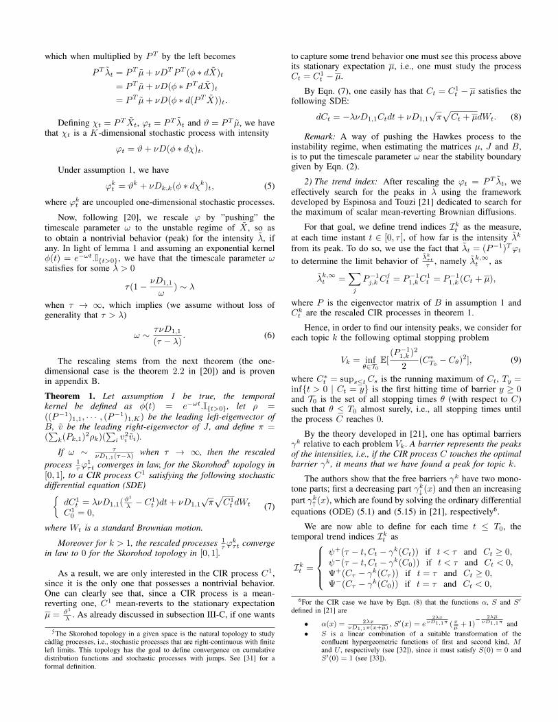
Algorithm 1 Trend detection algorithmInput: Hawkes process Xt, t ∈ [0, τ ], matrices J , B and µ1: Compute the leading left-eigenvector vT and eigenvalueν of J , and the topic intensities λt following Eqn. (3)2: Compute the leading right-eigenvector (P11, · · · , PK1),left-eigenvector (P−111 , · · · , P

−11K ) and eigenvalue D1,1 of B,

and the leading right-eigenvector v of J3: ”Push” λt to the instability regime following Eqn. (6)and calculate the CIR intensity Ct following Eqn. (8)4: Discretize [0, τ ] into T bins of size δ � 1for k = 1 to K do

5: Get the optimal barrier γk in {0, δ, 2δ, · · · , (T − 1)δ},following [21]for t = 1 to T do

5: Calculate the trend index Ik(t−1)δ using the optimalbarrier γk of the optimal stopping problem (9)

end for6: Calculate the topic trend index Ik =

∫ τ0Ikt dt =

δ∑Tt=1 Ik(t−1)δ

end forOutput: Trend indices Ik

centrality of the underlying social network as tool to createour trend indices, we not only use the topological propertiesof the social network in question but we reduce considerablythe dimension of the problem: we only have a one-dimensionalCIR process to study. Moreover, the complexity of the algo-rithm breaks down to three parts: 1) the resolution of the Koptimal barrier ODEs, which is of order O(Kδ ) where δ isthe time-discretization step, 2) the calculation of the left andright leading eigenvectors of J and B, which can be achievedfairly fast with iterative methods such as the power method,and 3) the matrix product in the calculation of µ, which hascomplexity O(NK).

IV. NUMERICAL EXAMPLES

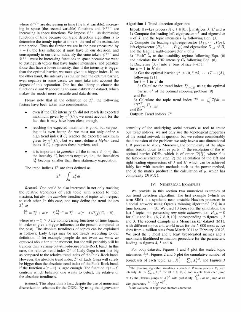
We provide in this section two numerical examples ofour trend detection algorithm. The first example (which weterm SIM) is a synthetic near unstable Hawkes processes ina social network using Ogata’s thinning algorithm7 [23] in atime horizon τ = 50. We used 10 topics for the simulation, thelast 5 topics not possessing any topic influence, i.e., Bc,k = 0for all c and k ∈ {6, 7, 8, 9, 10}, corresponding to figures 1, 2and 3. The second example is a MemeTracker dataset (MT),with different topics and world news for the 5, 000 most activesites from 4 million sites from March 2011 to February 20128.We used the 5 most and 5 least broadcasted memes and amaximum likelihood estimation procedure for the parameters,leading to figures 4, 5 and 6.

For both datasets, Figures 1 and 4 plot the scaled topicintensities λτt

τ , Figures 2 and 5 plot the cumulative number ofbroadcasts of each topic, i.e., X

k

t =∑iX

i,kt , and Figures 3

7The thinning algorithm simulates a standard Poisson process Pt withintensity M >

∑i,k λ

i,kt for all t ∈ [0, τ ] and selects from each jump

of Pt the Hawkes jumps of Xi,kt with probability λ

i,ktM

, or no jump at all

with probabilityM−

∑i,k λ

i,kt

M.

8Data available at http://snap.stanford.edu/netinf.

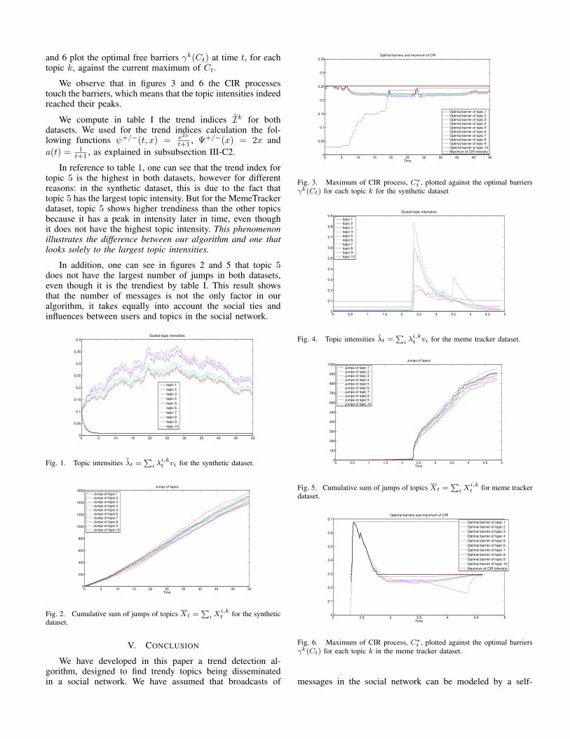
and 6 plot the optimal free barriers γk(Ct) at time t, for eachtopic k, against the current maximum of Ct.

We observe that in figures 3 and 6 the CIR processestouch the barriers, which means that the topic intensities indeedreached their peaks.

We compute in table I the trend indices Ik for bothdatasets. We used for the trend indices calculation the fol-lowing functions ψ+/−(t, x) = e2x

t+1 , Ψ+/−(x) = 2x anda(t) = 1

t+1 , as explained in subsubsection III-C2.

In reference to table 1, one can see that the trend index fortopic 5 is the highest in both datasets, however for differentreasons: in the synthetic dataset, this is due to the fact thattopic 5 has the largest topic intensity. But for the MemeTrackerdataset, topic 5 shows higher trendiness than the other topicsbecause it has a peak in intensity later in time, even thoughit does not have the highest topic intensity. This phenomenonillustrates the difference between our algorithm and one thatlooks solely to the largest topic intensities.

In addition, one can see in figures 2 and 5 that topic 5does not have the largest number of jumps in both datasets,even though it is the trendiest by table I. This result showsthat the number of messages is not the only factor in ouralgorithm, it takes equally into account the social ties andinfluences between users and topics in the social network.

0 5 10 15 20 25 30 35 40 45 500

0.05

0.1

0.15

0.2

0.25

0.3

0.35

0.4Scaled topic intensities

topic 1

topic 2

topic 3

topic 4

topic 5

topic 6

topic 7

topic 8

topic 9

topic 10

Fig. 1. Topic intensities λt =∑i λi,kt vi for the synthetic dataset.

0 5 10 15 20 25 30 35 40 45 500

200

400

600

800

1000

1200

1400

1600Jumps of topics

Time

Jumps of topic 1Jumps of topic 2Jumps of topic 3Jumps of topic 4Jumps of topic 5Jumps of topic 6Jumps of topic 7Jumps of topic 8Jumps of topic 9Jumps of topic 10

Fig. 2. Cumulative sum of jumps of topics Xt =∑iX

i,kt for the synthetic

dataset.

V. CONCLUSION

We have developed in this paper a trend detection al-gorithm, designed to find trendy topics being disseminatedin a social network. We have assumed that broadcasts of

0 5 10 15 20 25 30 35 40 45 500

0.05

0.1

0.15

0.2

0.25

0.3

0.35Optimal barriers and maximum of CIR

Time

Optimal barrier of topic 1Optimal barrier of topic 2Optimal barrier of topic 3Optimal barrier of topic 4Optimal barrier of topic 5Optimal barrier of topic 6Optimal barrier of topic 7Optimal barrier of topic 8Optimal barrier of topic 9Optimal barrier of topic 10Maximum of CIR Intensity

Fig. 3. Maximum of CIR process, C∗t , plotted against the optimal barriersγk(Ct) for each topic k for the synthetic dataset

0 0.5 1 1.5 2 2.5 3 3.5 4 4.5 50

0.1

0.2

0.3

0.4

0.5

0.6

0.7

0.8

0.9Scaled topic intensities

topic 1topic 2topic 3topic 4topic 5topic 6topic 7topic 8topic 9topic 10

Fig. 4. Topic intensities λt =∑i λi,kt vi for the meme tracker dataset.

0 0.5 1 1.5 2 2.5 3 3.5 4 4.5 50

100

200

300

400

500

600

700

800

900

1000Jumps of topics

Time

Jumps of topic 1Jumps of topic 2Jumps of topic 3Jumps of topic 4Jumps of topic 5Jumps of topic 6Jumps of topic 7Jumps of topic 8Jumps of topic 9Jumps of topic 10

Fig. 5. Cumulative sum of jumps of topics Xt =∑iX

i,kt for meme tracker

dataset.

2 2.5 3 3.5 4 4.5 50

0.1

0.2

0.3

0.4

0.5

0.6

0.7Optimal barriers and maximum of CIR

Time

Optimal barrier of topic 1










Maximum of CIR Intensity

Fig. 6. Maximum of CIR process, C∗t , plotted against the optimal barriersγk(Ct) for each topic k in the meme tracker dataset.

messages in the social network can be modeled by a self-

TABLE I. TREND INDICES FOR EACH DATASET.

DATASET I1 I2 I3 I4 I5 I6 I7 I8 I9 I10

SIM 0.0481 0.0414 0.0407 0.0433 0.0507 0.0148 0.0148 0.0148 0.0148 0.0148MT 0.1175 0.1090 0.1199 0.1229 0.1404 0.1035 0.1035 0.1035 0.1035 0.1035

exciting point process, namely a Hawkes process, which takesinto consideration the real broadcasting times of messages andthe interaction between users and topics.

We defined our idea of trendiness and derived trend indicesfor each topic being disseminated. These indices take intoconsideration the time between the actual trend detection andthe message broadcasts, the distance between the intensity ofbroadcasting and the maximum expected intensity of broad-casting, and the social network topology. This result is, tothe best of our knowledge, the first definition of relativetrendiness, i.e., a topic may not be very trendy in absolutenumber of broadcasts when compared to other topics, but hasstill rapid and significant number of broadcasts as compared toits expected behavior. Still, one can easily create an absolutetrend index for each topic in our trend detection algorithm,where all one needs to do is use the broadcasting intensitiesof each topic as surrogates for their trendiness. It is worthymentioning that these broadcast intensities also take intoconsideration the social network topology, or more precisely,the outgoing eigenvector centrality of each user, i.e., theirrespective influences on the social network.

The proposed trend detection algorithm is simple and usesstochastic control techniques in order to derive a free barrierfor the maximum expected broadcast intensity of each topic.This method is fast and aggregates all the information of thepoint process into a simple one-dimensional diffusion, thusreducing its complexity and the quantity of data necessary tothe detection - indispensable features if one is concerned withthe detection of trends in real-life social networks.

APPENDIX AASSUMPTIONS AND MAIN THEOREM

We now proceed to the proof of theorem 1, following theideas in [20]. According to section II, we have a multivariatelinear Hawkes process Xi,k

t with intensity of the form

λi,kt = µi,k +∑c

∑j

Bc,kJi,j

∫ t−

0

φ(t− s)dXj,cs , (10)

which in matrix form can be seen as

λt = µ+ J(φ ∗ dX)tB,

where µ is the intrinsic rate of dissemination, J is the user-user interaction matrix, B is the topic-topic interaction matrixand (φ ∗ dX)t is the N × K convolution matrix defined as(φ ∗ dX)i,kt =

∫ t0φ(t− s)dXi,k

s .

In order to prove our main rescaling convergence result,we make the following assumptions:

Assumption 2. The temporal kernel φ(t) is an exponentialfunction with timescale parameter ωτ

φ(t) = e−ωτ t.I{t>0}.

Remark: Assumption 2 is in fact a simplifying one, andone may use any temporal kernel satisfying the hypothesis in[20].

Assumption 3. The interaction matrices J and B can bediagonalized into J = v−1νv and B = ρDρ−1 and BT ⊗ Jhas only one maximal eigenvalue. Thus, in light of the decom-position for J and B, we have that J has left-eigenvectors therows of v, denoted by vTi , with associated eigenvalues νi; andB has right-eigenvectors the columns of ρ, denoted by ρk, withassociated eigenvalues Dk,k, i.e., vT is the N ×N matrix andρ is the K ×K matrix

vT =

. . .vT1 . . . vTN

. . .

and ρ =

(. . .

ρ1 . . . ρK. . .

).

Since the eigenvalues of BT ⊗ J are of the formviDk,k, (i, k), we assume without loss of generality thatν1 ≥ ν2 ≥ · · · ≥ νN and D1,1 > D2,2 ≥ D3,3 ≥ · · · ≥ DK,K ,and that the largest eigenvalues of J and B satisfy ν1 > 0 andD1,1 > 0.

Moreover, we also have that vT1 and ρ1 have nonnegativeentries by the Perron-Frobenius theorem, since J and B havenonnegative entries (this result remains true for the leadingright-eigenvector of J and the leading left-eigenvector of Bas well).

Remark: The assumption that J and B can be diagonalizedis in fact a simplifying one. One could use the Jordan blocks ofJ and B, on the condition that there exists only one maximaleigenvalue for BT ⊗ J . This assumption is verified if, forexample, the graph associated with B is strongly connected;which means that every topic influences the other topics, evenif it is in an undirected fashion (by influencing topics thatwill, in their turn, influence other topics, and so on). Onecan also develop a theory in the case of multiple maximaleigenvalues, but it will be much more complicated and theassociated stochastic control problem has not yet be solvedanalytically, hence numerical methods must be employed.

Assumption 4. We have that the timescale parameter ωτsatisfies, for some λ > 0,

τ(1− ν1D1,1

ωτ)→ λ

when τ →∞, which implies

ωτ ↘ ν1D1,1.

Appendix B is thus responsible for the proof of thefollowing theorem:

Theorem 2. Let X be the multivariate Hawkes process in[0, τ ] with intensity given by Eqn. (10), and let ϕi,kt =vTi

λτtτ ρk, where vTi and ρk are defined in assumption 3.

Under assumptions 2, 3 and 4 we have that

• If (i, k) 6= (1, 1) then ϕi,kt converges in law to 0 forthe Skorokhod topology in [0, 1] when τ →∞.

• Let vT1 and v1 be the leading left and right eigenvec-tors of J associated with the eigenvalue ν1 > 0, letρ1 and ρT1 be the leading right and left eigenvectorsof B associated with the eigenvalue D1,1 > 0, anddefine π = (

∑i v

21,ivi,1)(

∑k ρ

2k,1ρ1,k).

Thus, ϕ1,1t converges in law to the CIR process Ct

for the Skorokhod topology in [0, 1] when τ → ∞,where Ct, t ∈ [0, 1] satisfies the following stochasticdifferential equation{dCt = λν1D1,1(µλ − Ct)dt+ ν1D1,1

√π√CtdWt,

C0 = 0,


APPENDIX BPROOF OF THEOREM 2

A. Sketch of proof

We provide here a sketch of the proof:

1) We start by writing the equations satisfied by therescaled intensities ϕi,kt = vTi

λτtτ ρk and study their

first-order properties.2) Secondly, we define the new martingales Bi,kt and

show that they converge to a standard Brownianmotion.

3) Thirdly, we rewrite ϕ1,1t in a more suitable form, with

remainder terms Ut and Vt, and we show that theyconverge to 0.

4) Finally, we apply the convergence theorem 5.4 of[34] for limits of stochastic integrals with semimartin-gales.

B. Rescaling the Hawkes intensity

Let us begin by defining the one-dimensional stochasticprocesses

λi,kt = vTi λtρk,

which satisfy the one-dimensional equations

λi,kt = vTi µρk + vTi J(φ ∗ dX)tBρk

= µi,k + νiDk,k(φ ∗ λi,k)t + νiDk,k(φ ∗ vTi dMρk)t,(11)

with Mt = Xt −∫ t0λsds the compensated martingale asso-

ciated with the Hawkes process X and µi,k = vTi µρk. Usinglemma 2.1 of [20], we have that

λi,kt = µi,k+µi,k∫ t

0

Ψi,k(t−s)ds+

∫ t

0

Ψi,k(t−s)vTi dMsρk,

(12)where

Ψi,k(t) =∑n≥1

(νiDk,kφ(t))∗n,

with the nth convolution operator defined as

(νiDk,kφ(t))∗1 = νiDk,kφ(t), and

(νiDk,kφ(t))∗n = ((νiDk,kφ)∗(n−1) ∗ νiDk,kφ)t.

We have the following lemma for the convolutions Ψi,k:

Lemma 2. Let Ψi,k(t) =∑n≥1(νiDk,kφ(t))∗n, then under

assumption 2 we have that

Ψi,k(t) = νiDk,ke−ωτ (1−

νiDk,kωτ

)t.

Moreover, under assumptions 3 and 4 we have that

Ψ1,1(τt)→ ν1D1,1e−ν1D1,1λt

uniformly in [0, 1] when τ → ∞, and that there exists aconstant L > 0 such that for (i, k) 6= (1, 1) we have∫ t

0

Ψi,k(τ(t− s))ds ≤ L

τ. (13)

Proof: Under assumption 2, we have that

(νiDk,kφ(t))∗2 = (νiDk,k)2∫ t

0

e−ωτ (t−s)e−ωτsds

= (νiDk,k)2te−ωτ t

⇒ (νiDk,kφ(t))∗n = (νiDk,k)ntn−1

(n− 1)!e−ωτ t,

hence

Ψi,k(t) = e−ωτ t∑n≥1

νni Dnk,k

tn−1

(n− 1)!= νiDk,ke

−(1−νiDk,kωτ

)ωτ t.

Now, under assumptions 3 and 4, we have that τ(1 −ν1D1,1

ωτ) → λ and ωτ → ν1D1,1, which implies that there

exists a constant λ > 0 such that for every (i, k) 6= (1, 1)

ωτ (1− νiDk,k

ωτ) ≥ λ > 0 and τ(1− νiDk,k

ωτ)→∞.

Firstly, for t ∈ [0, 1], using the Lipschitz continuity of e−twe have that

|Ψ1,1(τt)− ν1D1,1e−ν1D1,1λt|

≤ (ν1D1,1)2λ( sups∈[0,1]

e−ν1D1,1λs)t|ωττ(1− ν1D1,1

ωτ)− ν1D1,1λ|

≤ (ν1D1,1)2λ|ωττ(1− ν1D1,1

ωτ)− ν1D1,1λ| → 0

when τ → ∞, which implies that Ψ1,1(τt) →ν1D1,1e

−ν1D1,1λt uniformly in [0, 1].

At last, for (i, k) 6= (1, 1), we have that∫ t

0

Ψi,k(τ(t− s))ds = νiDk,k1− e−tτωτ (1−

νiDk,kωτ

)

τωτ (1− νiDk,kωτ

)≤ L

τ

where L > 0 is a large enough positive constant.

Let us now define the one-dimensional rescaled stochasticprocesses, for t ∈ [0, 1],

ϕi,kt =vTi λτtρk

τ,

which clearly satisfies

ϕt = vλτtτρ. (14)

We have the following lemma concerning the first orderproperties of ϕt:

Lemma 3. Let us define the 1×N row vector v�2i such that(v�2i )j = v2i,j and the K × 1 vector ρ�2k such that (ρ�2k )c =ρ2c,k. We have

1) ϕi,kt satisfies the following equation

ϕi,kt = µi,k(1

τ+

∫ t

0

Ψi,k(τ(t− s))ds)

+

∫ t

0

Ψi,k(τ(t− s))√

(v�2i )Tλτsτρ�2k dBi,ks , (15)

where

Bi,kt =√τ

∫ t

0

vTi dMτsρk√(v�2i )Tλτsρ

�2k

=

∫ t

0

vTi dMτsρk√(v�2i )T v−1ϕsρ−1ρ

�2k

is a L2 martingale.2) If (i, k) 6= (1, 1), then

E[ϕi,kt ] ≤ L

τ,

where L > 0 is a large enough positive constant.Moreover, we also have that

E[ϕ1,1t ] ≤ L.

Proof:

1) We have that

ϕi,kt =1

τµi,k +

1

τµi,k

∫ τt

0

Ψi,k(τt− s)ds

+1

τ

∫ τt

0

Ψi,k(τt− s)vTi dMsρk

=1

τµi,k + µi,k

∫ t

0

Ψi,k(τ(t− s))ds

+

∫ t

0

Ψi,k(τ(t− s))vTi dMτsρk

=1

τµi,k + µi,k

∫ t

0

Ψi,k(τ(t− s))ds

+

∫ t

0


(v�2i )Tλτsτ s

ρ�2kvTi√τdMτsρk√

(v�2i )Tλτsρ�2k

=1

τµi,k + µi,k

∫ t

0

Ψi,k(τ(t− s))ds

+

∫ t

0


(v�2i )Tλτsτ s

ρ�2k dBi,ks .

As λτsτ = v−1ϕsρ

−1 by Eqn. (14), we have the result.

2) Since Bi,kt is a martingale, we have that

E[ϕi,kt ] =1

τµi,k +

1

τµi,k

∫ τt

0

Ψi,k(τt− s)ds

=1

τµi,k + µi,k

∫ t

0

Ψi,k(τ(t− s))ds,

which together with lemma 2 gives us the result.

Remark: We can assume, without loss of generality,that there exists a c > 0 such that min(i,k) v

Ti µρk =

min(i,k) µi,k ≥ c, since vTi µρk = µi,k = 0 ⇒ E[ϕi,kt ] = 0

by lemma 3, which implies ϕi,kt = 0 almost surely for allt ≥ 0 by the fact that ϕi,kt ≥ 0 for all t ≥ 0.

C. Second order properties

Regarding the second order properties of Bi,kt and ϕi,kt ,we have the following lemma:

Lemma 4. For each (i, k) let [Bi,k]t be the quadratic varia-tion of the martingale Bi,kt . We have that

1)

[Bi,k]t = t+1

τ

∫ τt

0

(v�2i )T dMsρ�2k

(v�2i )Tλsρ�2k

. (16)

2)E[(ϕi,kt )2] ≤ L (17)

for a constant L > 0.3) Moreover, if (i, k) 6= (1, 1), then

E[(ϕi,kt )2] ≤ L

τ2

for a constant L > 0.

Proof:

1) Since the Hawkes process X does not have more thanone jump at each time, we have that

[M i,k,M j,c]t = Xi,kt I{(i,k)=(j,c)},

which by its turn implies

[vTi Mρk]t = (v�2i )TXtρ�2k .

We have by lemma 3 that

Bi,kt =√τ

∫ t

0

vTi dMτsρk√(v�2i )Tλτsρ

�2k

=1√τ

∫ τt

0

vTi dMsρk√(v�2i )Tλsρ

�2k

,

hence

[Bi,k]t =1

τ

∫ τt

0

(v�2i )T dXsρ�2k


=1

τ

∫ τt

0



ds+1

τ

∫ τt

0



= t+1

τ

∫ τt

0



.

2) Using the fact that (a + b + c)2 ≤ 3(a2 + b2 + c2),we have by Eqn. (15) and lemma 2 that

(ϕi,kt )2 ≤ 3

((µi,k)2

τ2+ (µi,k)2(

∫ t

0

Ψi,k(τ(t− s))ds)2

+ (

∫ t

0


(v�2i )T v−1ϕsρ−1ρ�2k dBi,ks )2

)≤ L′ + 3(

∫ t

0

Ψi,k(τ(t− s))√(v�2i )T v−1ϕsρ−1ρ

�2k dBi,ks )2.

Since Ψi,k(τ(t− s)) = Ψi,k(τt)Ψi,k(−τs), we havethen

(ϕi,kt )2 ≤ L′ + 3(

∫ t

0

Ψi,k(τ(t− s))√(v�2i )T v−1ϕsρ−1ρ

�2k dBi,ks )2

= L′ + 3Ψ2i,k(τt)(Zi,kt )2,

with Zi,kt =∫ t0

Ψi,k(−τs)√

(v�2i )T v−1ϕsρ−1ρ�2k dBi,ks

a martingale. By lemmas 8 and 3 we have that

E[(ϕi,kt )2] ≤ L′ + 3Ψ2i,k(τt)

∫ t

0

Ψ2i,k(−τs)

(v�2i )T v−1E[ϕs]ρ−1ρ�2k ds

= L′ + 3

∫ t

0

Ψ2i,k(τ(t− s))

(v�2i )T v−1E[ϕs]ρ−1ρ�2k ds ≤ L.

3) For (i, k) 6= (1, 1), we have from Eqn. (12), lemma2 and the inequality (a+ b+ c)2 ≤ 3(a2 + b2 + c2)that

(λi,kt )2 ≤ L′ + 3(

∫ t

0

Ψi,k(t− s)vTi dMsρk)2.

One can promptly see by lemma 3 that E[λi,kt ] =(v−1E[λt]ρ

−1)i,k ≤ L′′′. Hence using lemma 8 andthe same calculation of the previous item gives

E[(λi,kt )2] ≤ L′ + 3

∫ t

0

Ψ2i,k(t− s)(v�2i )TE[λs]ρ

�2k ds

≤ L′′(1 +

∫ t

0

Ψ2i,k(t− s)ds) ≤ L

for a constant L > 0. Thus E[(ϕi,kt )2] =E[(λi,kτt )

2]τ2 ≤

Lτ2 , as desired.

We derive next the convergence properties of the martin-gales Bi,kt and the rescaled process ϕi,kt , (i, k) 6= (1, 1).

Lemma 5. We have that

1) For every (i, k), Bi,kt converges in law to a standardBrownian motion for the Skorohod topology in [0, 1]when τ →∞.

2) If (i, k) 6= (1, 1), then ϕi,kt converges in law to 0 forthe Skorohod topology in [0, 1] when τ →∞.

Proof:

1) By Eqn. (16) we have for t ∈ [0, 1]

E[([Bi,k]t − t)2] = E[(1

τ

∫ τt

0



)2]

≤ 1

τ2E[

∫ τt

0

d[(v�2i )TMρ�2k ]s((v�2i )Tλsρ

�2k

)2 ]

=1

τ2E[

∫ τt

0

(v�4i )Tλsρ�4k ds(


)2 ]

≤ ||v�2i ||.||ρ�2k ||.

1

τ2E[

∫ τt

0

ds


]

≤ L 1

τ2

∫ τt

0

dt ≤ L

τ

for some L > 0 by lemma 9.Thus, by Markov’s inequality we have that for allε > 0 and for all t ∈ [0, 1]

P(|[Bi,k]t − t| ≥ ε) ≤L

τε2→ 0 when τ →∞,

which shows that, for every t ∈ [0, 1], [Bi,k]t con-verges in probability towards t when τ →∞.Since Bi,k has uniformly bounded jumps because Xand λ have uniformly bounded jumps, we have bytheorem V III.3.11 of [35] that Bi,kt converges inlaw to a standard Brownian motion for the Skorohodtopology in [0, 1] when τ →∞.

2) Since supt∈[0,1] E[ϕi,kt ] → 0 when τ → ∞by lemma 3, we have by Eqn. (15) that weonly need to prove the convergence of Zi,kt =∫ t0

Ψi,k(τ(t − s))g(ϕs)dBi,ks , where g(ϕs) =√

(v�2i )T v−1ϕsρ−1ρ�2k satisfies |g(ϕs)| ≤ C(1 +

||ϕs||) for some C > 0.Since Ψi,k(τ(t − s)) is an exponential function bylemma 2, we have that assumption 4 implies thatΨi,k(τ(t − s)) satisfies all hypothesis of lemma 10,and as consequence we have that Zi,kt converges inlaw to 0 for the Skorohod topology in [0, 1] whenτ →∞, which concludes the proof.

D. Convergence of ϕ1,1t

After studying the asymptotic behavior of the martingaleBt and the rescaled processes ϕi,kt for (i, k) 6= (1, 1), we studythe asymptotic behavior of ϕ1,1

t . We start by rewriting it in amore convenient form, using Eqn. (15):

ϕ1,1t = µ1,1(

1

τ+

∫ t

0

Ψ1,1(τ(t− s))ds) (18)

+

∫ t

0

ν1D1,1e−ν1D1,1λ(t−s)

√πϕ1,1

s dB1,1s

+ Ut + Vt, (19)

where π = (∑i v

21,i(v

−1)i,1)(∑k ρ

2k,1(ρ−1)1,k),

Ut =

∫ t

0

Ψ1,1(τ(t−s))(√

(v�21 )T v−1ϕsρ−1ρ�21 −

√πϕ1,1

s )dB1,1s .

(20)

and

Vt =

∫ t

0

(Ψ1,1(τ(t−s))−ν1D1,1e

−ν1D1,1λ(t−s))√

πϕ1,1s dB1,1

s

(21)

We begin by studying the asymptotic behavior of Ut inEqn. (20) and Vt in (21).

Lemma 6. We have that Ut defined in Eqn. (20) converges inlaw to 0 for the Skorohod topology in [0, 1] when τ →∞.

Proof: Let us define the martingale Zt =∫ t0

Ψ1,1(−τs)(√

(v�21 )T v−1ϕsρ−1ρ�21 −

√πϕ1,1

s )dB1,1s ,

such that Ut = Ψ1,1(τt)Zt. Using the product formula forsemimartingales and the fact that Ψ1,1 has bounded variation,we have that

Ut =

∫ t

0

∂tΨ1,1(τs)Zsds+

∫ t

0

Ψ1,1(τs)dZs = Vt +Wt,

where Vt =∫ t0∂tΨ1,1(τs)Zsds has bounded variation and

Wt =∫ t0

Ψ1,1(τs)dZs is a martingale with quadratic variation[W ]t satisfying by lemma 8

[W ]t =

∫ t

0

Ψ21,1(τs)d[Z]s

=

∫ t

0

Ψ21,1(τs)Ψ2

1,1(−τs)

(

√(v�21 )T v−1ϕsρ−1ρ

�21 −

√πϕ1,1

s )2d[B1,1]s

=

∫ t

0

(

√(v�21 )T v−1ϕsρ−1ρ

�21 −

√πϕ1,1

s )2d[B1,1]s.

Thus, using the fact that√a+ b−

√b ≤ a

2√b

for a, b > 0,we have by lemma 4

E[[W ]t] = E[

∫ t

0

(

√(v�21 )T v−1ϕsρ−1ρ

�21 −

√πϕ1,1

s )2ds]

≤ E[

∫ t

0

((v�21 )T v−1ϕsρ−1ρ�21 − πϕ1,1

s )2

4πϕ1,1s

ds]

≤ L2E[

∫ t

0

(∑

(i,k)6=(1,1) ϕi,ks )2

4πϕ1,1s

ds]

for some constant L > 0 by lemma 11. Since ϕ1,1s ≥ µ1,1

τ ≥cτ > 0, we have by lemma 4 that for t ∈ [0, 1]

E[[W ]t] ≤τL2

4πcE[

∫ t

0

(∑

(i,k)6=(1,1)

ϕi,ks )2ds]

≤ τL(NK − 1)

4πcE[

∫ t

0

∑(i,k)6=(1,1)

(ϕi,ks )2ds]

=τL(NK − 1)

4πc

∫ t

0

∑(i,k)6=(1,1)

E[(ϕi,ks )2]ds

≤ τL2(NK − 1)2

4πc

∫ t

0

1

τ2ds =

L′t

τ≤ L′

τ

for L′ = L2(NK−1)24πc .

Thus, by Markov’s inequality we have that for all ε > 0and for all t ∈ [0, 1]

P([W ]t ≥ ε) ≤L′

ε(

1

τ2+

1

τ)→ 0 when τ →∞,

which proves that [W ]t converges in probability to 0 for allt ≥ 0.

Since W has uniformly bounded jumps, we have bytheorem V III.3.11 of [35] that Wt converges in law to 0for the Skorohod topology in [0, 1] when τ →∞.

Now, regarding Vt, we have that since |∂tΨ1,1(τt)| ≤ Cfor some constant C > 0,

E[(Vt − Vs)2] = E[(

∫ t

s

∂tΨ1,1(τu)Zudu)2]

≤ C2(t− s)2E[( supu∈[s,t]

Zu)2] ≤ C ′(t− s)2E[[Z]t]

by the Burkholder-Davis-Gundy inequality. Since by lemma 8

[Z]t =

∫ t

0

Ψ21,1(−τs)(

√(v�21 )T v−1ϕsρ−1ρ

�21 −

√πϕ1,1

s )2d[B1,1]s

and Ψ1,1(−τs) ≤ C for some constant C > 0, we have usingthe same calculations as before and choosing s = 0 that fort ∈ [0, 1]

E[V 2t ] ≤ C ′t2E[[Z]t] ≤

C ′′

τ2,

which easily implies that (Vt1 , · · · , Vtn) → 0 in distributionfor every (t1, · · · , tn) ∈ [0, 1]n when τ → ∞, i.e., we havethe convergence of the finite-dimensional distribution of Vt to0 when τ →∞.

Moreover, since E[(Vt − Vs)2] ≤ C ′′′(t− s)2, we have bythe Kolmogorov criterion for tightness that Vt is tight for theSkorohod topology in [0, 1], which implies that Vt convergesin law to 0 for the Skorohod topology in [0, 1] when τ →∞.

Hence, we clearly have that Ut = Vt + Wt converges inlaw to 0 for the Skorohod topology in [0, 1] when τ →∞.

Lemma 7. We have that Vt defined in Eqn. (21) converges inlaw to 0 for the Skorohod topology in [0, 1] when τ →∞.

Proof: Define the function

fτ (t) = Ψ1,1(τt)− ν1D1,1e−ν1D1,1λt

= ν1D1,1

(e−ωττ(1−

ν1D1,1ωτ

)t − e−ν1D1,1λt

).

By assumption 4, that there exists a C > 0 such that

1) supτ supt |fτ (t)| ≤ C,2) Since fτ is a difference of exponential functions, we

can assume without loss of generality that |fτ (z)| ≤C(| 1z | ∧ 1),

3) Applying lemma 4.7 of [20] we have that for any0 < ε < 1, there exists Cε > 0 such that for everyt, s

supτ

∫R

(fτ (t− u)− fτ (s− u))2du ≤ Cε|t− s|1−ε,

4) Since

f2τ (t) = ν21D21,1

(Ψ2

1,1(τt) + e−2ν1D1,1λt

− 2Ψ1,1(τt)e−ν1D1,1λt

),

we have that∫R+

f2τ (t)dt = ν21D21,1

(1

2ωττ(1− ν1D1,1

ωτ)

+1

2ν1D1,1λ− 2

1

ωττ(1− ν1D1,1

ωτ) + ν1D1,1λ

)→ 0.

5) Since, for α > 0, e−αt satisfies |e−αt − e−αs| ≤α|t − s|, we easily have that there exists a constantC > 0 such that

|fτ (t)− fτ (s)| ≤ Cτ |t− s|.

Hence, fτ satisfies all hypothesis of lemma 10. Moreover,

g(ϕs) =

√πϕ1,1

s easily satisfies

|g(ϕt)| ≤ C(1 + ||ϕt||).

We can thus apply lemma 10 to conclude the proof.

We have arrived to the final step of the proof: bylemma 2, we have that µ1,1

∫ t0

Ψ1,1(τ(t − s))ds convergesuniformly in [0, 1] to µ1,1

∫ t0ν1D1,1e

−ν1D1,1λ(t−s)ds =

µ1,1( 1−e−ν1D1,1λt

λ ), when τ →∞.

Moreover, by lemma 5 we have that B1,1t converges in law

to a standard Brownian motion for the Skorohod topology in[0, 1] when τ → ∞, and by lemmas 6 and 7 we have thatUt and Vt converge in law to 0 for the Skorohod topology in[0, 1] when τ →∞.

As in [20], since Ut and Vt converge to a deterministiclimit, we get the convergence in law, for the product topology,of the triple (Ut, Vt, B

1,1t ) to (0, 0,Wt) with W a standard

Brownian motion. The components of (0, 0,Wt) being contin-uous, the last convergence also takes place for the Skorohodtopology on the product space.

Thus, we have by theorem 5.4 of [34] that ϕ1,1t converges

in law to the limit process Ct for the Skorohod topology in[0, 1] when τ →∞, where Ct is the unique solution of

Ct = µ1,1(1− e−ν1D1,1λt

λ)

+ ν1D1,1

∫ t

0

e−ν1D1,1λ(t−s)√πCsdWs,


By a simple calculation, we have that Ct satisfies the

following stochastic differential equation

dCt = ν1D1,1µ1,1e−ν1D1,1λtdt

+ ν1D1,1

(− ν1D1,1λ

∫ t

0

e−ν1D1,1λ(t−s)√πCsdWsdt

+√πCtdWt

)= ν1D1,1µ

1,1e−ν1D1,1λtdt

+ ν1D1,1

((µ1,1(1− e−ν1D1,1λt)− λCt)dt+

√πCtdWt

)= ν1D1,1λ(

µ1,1

λ− Ct)dt+ ν1D1,1

√πCtdWt.

Remark: One promptly has that the columns of v−1 arethe right-eigenvectors of J and that the rows of ρ−1 are theleft-eigenvectors of B, thus π > 0 can be rewritten as

π = (∑i

v21,ivi,1)(∑k

ρ2k,1ρ1,k),

where vT1 is the leading left-eigenvector of J , v1 is the right-eigenvector of J , ρ1 is the leading right-eigenvector of Band ρT1 is the leading left-eigenvector of B. Moreover, by thePerron-Frobenius theorem we have that v, v, ρ and ρ havenonnegative entries.

Remark: In the one-dimensional case, we clearly have thatπ = 1, retrieving thus the same result as in [20].

APPENDIX CADDITIONAL LEMMAS

Lemma 8. Let f : MN×K(R+) → R+ and g :MN×K(R+)→ R+ be functions satisfying for some constantC > 0

|f(ϕt)| ≤ C(1 + ||ϕt||) and |g(ϕt)| ≤ C(1 + ||ϕt||),

let h : R→ R and r : R→ R be continuous functions and letZ1t and Z2

t be L2 martingales such that [Z1, Z2]t = t+Mt,where Mt is a martingale.

Defining z1t =∫ t0h(s)f(ϕs)dZ

1s and z2t =∫ t

0r(s)g(ϕs)dZ

2s we have that

E[z1t z2t ] =

∫ t

0

h(s)r(s)E[f(ϕs)g(ϕs)]ds.

Moreover, if Zt is a L2 semimartingale, we have that thestochastic process Yt =

∫ t0h(s)f(ϕs)dZs satisfies

[Y ]t =

∫ t

0

h2(s)f2(ϕs)d[Z]s and E[Y 2t ] ≤ E[[Y ]t].

Lemma 9. Let X be a N×K matrix with nonnegative entries,vT 6= 0 be a 1 ×N row vector with nonnegative entries andρ 6= 0 be a K × 1 vector with nonnegative entries. Then

(v�2)TXρ�2 ≤ ||v||.||ρ||.vTXρ.

Proof: Define the row vector vT = vT

||v|| and the vectorρ = ρ

||ρ|| , such that vTi ≤ 1 and ρk ≤ 1, which implies (vi)2 ≤

vi and (ρk)2 ≤ ρk. Then

(v�2)TXρ�2 = ||v||2.||ρ||2∑i,k

v2iXi,kρ2k

≤ ||v||2.||ρ||2.∑i,k

viXi,kρk

= ||v||.||ρ||.∑i,k

viXi,kρk = ||v||.||ρ||vTXρ.

This lemma can be proven using the ideas in [20] (see theproof of the convergence for the rescaled process (Y Tt )t∈[0,1]at the beginning of page 18, corollaries 4.1, 4.2, 4.3, 4.4 andlemma 4.7).

Lemma 10. Let fτ : R+ → R be a sequence of functions suchthat

1) There exists a constant C > 0 such thatsupτ supt∈R |fτ (t)| ≤ C,

2) There exists a constant C > 0 such that for all τ

|fτ (t)− fτ (s)| ≤ Cτ |t− s|,

3) For any 0 < ε < 1, there exists Cε > 0 such that forevery t, s

supτ

∫R

(fτ (t− u)− fτ (s− u))2du ≤ Cε|t− s|1−ε,

4)∫R+ f

2τ (s)ds→ 0 when τ →∞, and

5) There exists a constant C > 0 such thatsupτ |fτ (z)| ≤ C(| 1z | ∧ 1).

Let g : MN×K(R+) → R be a function satisfying forsome constant C > 0

|g(ϕt)| ≤ C(1 + ||ϕt||),

and define Y i,k,τt =∫ t0fτ (t− s)g(ϕs)dB

i,ks .

We have that Y i,k,τt converges in law to 0 for the Skorohodtopology in [0, 1] when τ →∞.

Lemma 11. Let π = (∑i v

21,i(v

−1)i,1)(∑k ρ

2k,1(ρ−1)1,k). We

have that

(v�21 )T v−1ϕtρ−1ρ�21 ≤ πϕ1,1

t + L∑

(i,k)6=(1,1)

ϕi,kt

for some constant L > 0.

Proof: Let us define the 1 × N row vector V T =(v�21 )T v−1 and the K × 1 vector R = ρ−1ρ�21 , such that

V Tj =∑i

v21,iv−1i,j and Rc =

∑k

ρ−1c,kρ2k,1.

Thus

(v�21 )T v−1ϕtρ−1ρ�21 =

∑j,c

V Tj ϕj,ct Rc

= πϕ1,1t +

∑(j,c)6=(1,1)

V Tj ϕj,ct Rc

≤ πϕ1,1t + L

∑(i,k) 6=(1,1)

ϕi,kt

for a constant L > 0.

REFERENCES

[1] J. Kleinberg, “Bursty and hierarchical structure in streams,” In Proceed-ings of the ninth ACM SIGKDD international conference on Knowledgediscovery and data mining, pp. 91–101, 2002.

[2] X. Wang, C. Zhai, and R. S. X. Hu, “Mining correlated bursty topicpatterns from coordinated text streams,” In Proceedings of the ninthACM SIGKDD international conference on Knowledge discovery anddata mining, 2007.

[3] M. Cataldi, L. D. Caro, , and C. Schifanella, “Emerging topic detectionon twitter based on temporal and social terms evaluation,” In Proceed-ing of the 10th International Workshop on Multimedia Data Mining(MDMKDD), 2010.

[4] T. Takahashi, R. Tomioka, and K. Yamanishi, “Discovering emergingtopics in social streams via link anomaly detection,” In Proceeding ofthe 11th IEEE International Conference on Data Mining (ICDM), 2011.

[5] J. Goldenberg, B. Libai, and E. Muller, “Using complex systems anal-ysis to advance marketing theory development,” Academy of MarketingScience Review, 2001.

[6] D. Kempe, J. Kleinberg, and E. Tardos, “Maximizing the spread ofinfluence through a social network,” In Proceedings of the ninth ACMSIGKDD international conference on Knowledge discovery and datamining, pp. 137–146, 2003.

[7] H. P. Young, “The dynamics of social innovation,” Proc Natl Acad SciUSA, vol. 108, no. Suppl. 4, pp. 21 285–21 291, 2011.

[8] Y. Altshuler, W. Pan, and A. Pentland, “Trends prediction using socialdiffusion models,” Social Computing, Behavioral - Cultural Modelingand Prediction, vol. 7227, pp. 97–104, 2008.

[9] R. Crane and D. Sornette, “Robust dynamic classes revealed by mea-suring the response function of a social system,” Proceedings of theNational Academy of Sciences, vol. 105, no. 41, pp. 15 649–15 653,2008.

[10] L. Li and H. Zha, “Dyadic event attribution in social networks withmixtures of Hawkes processes,” Proceedings of 22nd ACM InternationalConference on Information and Knowledge Management (CIKM), 2013.

[11] S.-H. Yang and H. Zha, “Mixture of mutually exciting processes forviral diffusion,” Proceedings of the 30th International Conference onMachine Learning (ICML), 2013.

[12] I. Valera, M. Gomez-Rodriguez, and K. Gummadi, “Modeling adoptionand usage frequency of competing products and conventions in socialmedia,” Workshop in Networks: From Graphs to Rich Dat at NeuralInformation Processing Systems Conference (NIPS), 2014.

[13] M. Farajtabar, N. Du, M. Gomez-Rodriguez, I. Valera, H. Zha, andL. Song, “Shaping social activity by incentivizing users,” In proceedingsof Neural Information Processing Systems Conference (NIPS), 2014.

[14] J. Cheng, L. Adamic, A. Dow, J. Kleinberg, and J. Leskovec, “Can cas-cades be predicted?” In Proceedings of ACM International Conferenceon World Wide Web (WWW), 2014.

[15] J. Leskovec, L. Backstrom, and J. Kleinberg, “Meme-tracking and thedynamics of the news cycle,” In Proceedings of the ninth ACM SIGKDDinternational conference on Knowledge discovery and data mining, pp.497–506, 2009.

[16] R. Dawkins, The Selfish Gene, 2nd ed. Oxford University Press, 1989.[17] A. G. Hawkes, “Spectra of some self-exciting and mutually exciting

point processes,” Biometrika, vol. 58, pp. 83–90, 1971.[18] T. Liniger, “Multivariate Hawkes processes,” ETH Doctoral Disserta-

tion, no. 18403, 2009.

[19] M. E. J. Newman, “The mathematics of networks,” Notes, 2006.[20] T. Jaisson and M. Rosenbaum, “Limit theorems for nearly unstable

hawkes processes,” ArXiv: 1310.2033, 2013.[21] G.-E. Espinosa and N. Touzi, “Detecting the maximum of a scalar dif-

fusion with negative drift,” SIAM Journal on Control and Optimization,vol. 50, no. 5, pp. 2543–2572, 2012.

[22] D. J. Daley and D. Vere-Jones, An introduction to the theory of pointprocesses, ser. Springer series in Statistics. Springer, 2005.

[23] Y. Ogata, “On lewis simulation method for point processes,” IEEETransactions on Information Theory, vol. 27, no. 1, pp. 23–31, 1981.

[24] A. G. Hawkes and D. Oakes, “A cluster process representation of aself-exciting point process,” J. Appl. Prob., vol. 11, pp. 493–503, 1974.

[25] P. Bremaud and L. Massoulie, “Stability of nonlinear Hawkes pro-cesses,” The Annals of Probability, vol. 24, no. 3, pp. 1563–1588, 1996.

[26] M. Kivela, A. Arenas, M. Barthelemy, J. P. Gleeson, Y. Moreno, andM. A. Porter, “Multilayer networks,” Journal of Complex Networks,no. 2, 2014.

[27] P. Holme and J. Saramaki, (eds.), Temporal Networks. Berlin: Springer,2013.

[28] E. Bacry and J.-F. M. S. Gaıffas, “Concentration for matrix martingalesin continuous time and microscopic activity of social networks,” ArXiv:1412.7705, 2014.

[29] J. C. Cox, J. E. Ingersoll, and S. A. Ross, “A theory of the term structureof interest rates,” Econometrica, vol. 53, pp. 385–407, 1985.

[30] D. F. Gleich, “Pagerank beyond the web,” ArXiv: 1407.5107, 2014.[31] P. Billingsley, Convergence of probability measures, ser. Wiley series

in Probability and Statistics. New York: Wiley, 2009, vol. 493.[32] M. Abramowitz and I. A. Stegun, Handbook of Mathematical Func-

tions: with Formulas, Graphs, and Mathematical Tables. New York:Dover, 1974.

[33] A. Kuznetsov, “Solvable markov processes,” Ph.D. dissertation, Univer-sity of Toronto, 2004.

[34] T. G. Kurtz and P. Protter, “Weak limit theorems for stochastic integralsand stochastic differential equations,” The Annals of Probability, vol. 19,no. 3, pp. 1035–1070, 1991.

[35] J. Jacod and A. N. Shiryaev, Limit theorems for stochastic processes.Berlin: Springer-Verlag, 1987, vol. 288.

trend detection in social networks using hawkes processes

Documents