water

Article

Tree-Type Irrigation Pipe Network Planning andDesign Method Using ICSO-ASV

Zhen Li 1,2, Zijian Lin 1, Shilei Lyu 1,2,*, Zhiwei Wei 1 and Heqing Huang 1

1 College of Electronic Engineering, South China Agricultural University, Guangzhou 510642, China;lizhen@scau.edu.cn (Z.L.); lamziqam@stu.scau.edu.cn (Z.L.); weizhiwei@stu.scau.edu.cn (Z.W.);huangheqing@stu.scau.edu.cn (H.H.)

2 Division of Citrus Machinery, China Agriculture Research System, Guangzhou 510642, China* Correspondence: lvshilei@scau.edu.cn; Tel.: +86-159-2019-1600

Received: 28 May 2020; Accepted: 3 July 2020; Published: 14 July 2020�����������������

Abstract: Research on tree-type irrigation pipe networks is an important component of agriculturalwater-saving projects. The optimal design of tree-type irrigation pipe networks is a key aspectregarding the profitability of irrigated agriculture. Meanwhile, swarm intelligence optimizationalgorithms have good computational ability and can be applied to solve many optimization problemsin agricultural engineering. To identify the lowest investment cost for a pipe network, this studydefined the concept of an upper water node to ensure the connectivity of tree-type irrigation pipenetworks, and therefore, improve the pipe network planning model without using preliminary networkconnection diagrams. In addition, this study proposed an improved chicken swarm optimizationalgorithm (Improved Chicken Swarm Optimization using Adaptive Search and Variation, ICSO-ASV),which was applied to solve 12 test functions of different dimensions. The test results show that,compared to the traditional chicken swarm algorithm and other algorithms in the control group,the ICSO-ASV algorithm could effectively improve the global search capability. Finally, the ICSO-ASValgorithm was used to plan and design 15-node and 40-node pipe networks. The calculation resultsshow that the average investment costs of the two pipe networks generated by the ICSO-ASValgorithm were 42.20% and 31.09% lower than those generated by the traditional chicken swarmalgorithm, which further verified the feasibility of applying ICSO-ASV to design tree-type irrigationpipe networks. Thus, the design method proposed in this study can solve the optimal problems oftree-type irrigation pipe networks with varying topologies. The optimal solutions can be generatedautomatically using the ICSO-ASV algorithm if essential parameters of the pipe network planningmodel are provided.

Keywords: tree-type irrigation pipe network; pipe network deployment; pipe diameter optimization;ICSO-ASV

1. Introduction

Compared to traditional open-channel water distribution methods, irrigation pipe networkshave the characteristics of an improved land utilization rate, reduced loss to evaporation andleakage, and high efficiency of water use. Such networks are therefore widely used in agriculturalwater-saving projects and represent the trend of future high-efficiency water-saving developments [1].Compared to ring-shaped irrigation pipe networks, tree-type irrigation pipe networks have tree-typepipe distributions, and therefore, the advantages of being structurally simple, saving material, and beingeasy to manage; such a system is therefore suitable for medium and small irrigation pipe networks [2].Studies on tree-type irrigation pipe networks have primarily focused on the optimal design of pipenetwork deployment planning and pipe diameter selection with the objective of minimizing the

Water 2020, 12, 1985; doi:10.3390/w12071985 www.mdpi.com/journal/water

Water 2020, 12, 1985 2 of 18

investment cost of the pipe network while satisfying the requirements of pipeline flow, flow rate,and node water pressure [3]. Pipe network deployment planning refers to finding the pipe connectionswith the shortest total pipe length under the premise of meeting the single-point water supply principleof a tree-type pipe network; here, pipe diameter selection refers to finding the pipe diameter with thelowest cost under the premise of meeting the water supply connectivity requirement of a tree-typepipe network.

In industry, methods such as graph theory [4] and orthogonal experiments [5] have been exploredto solve the problems of pipe network deployment planning; for example, differential [6], dynamicplanning [7], and economic flow rate [8] methods have been applied to optimize pipe diameterselection. Traditional optimization methods involve complicated calculations, have low solutionefficiencies, and are not versatile, which, to a certain degree, limits the application of pipe networkoptimization methods in actual engineering projects. Swarm intelligence optimization algorithmsare types of meta-heuristic algorithms that simulate the swarm intelligence behavior of a gregariouscolony [9]. They can obtain optimal solutions to optimization problems of engineering projects bysimulating the behaviors of cooperation and competition among individuals in the gregarious colony.These algorithms are currently applied to study pipe network planning and design, with the pipenetwork planning and design problem described as a discrete combinatorial optimization problemthat uses the pipe network deployment between water nodes and the pipe diameter size as decisionvariables. Thus, the pipe network planning model can be taken as a high-dimensional nonlinearfunction on computational aspects, and the swarm intelligence optimization algorithms are excellenttools used for solving the complicated function through searching the global optimal solution in thefield of feasible function solutions. For irregular irrigation pipe networks, Li et al. [10] proposed a pipenetwork planning model to simultaneously optimize pipe network deployment and the pipe diameter.Zhou et al. [11] used an improved single-parent genetic algorithm to optimize the design of a tree-typepipe network. Ma et al. [12] used the harmony search algorithm to solve for the optimal diametercombination. Chen et al. [13] solved the pipe network model based on the firefly algorithm and appliedthe result to the optimal design of a drip irrigation pipe network. Most of the above-mentioned studiesused intelligent optimization algorithms for the synchronous design of the pipe network deploymentand the pipe diameter; however, the optimization of the pipe network deployment still requires aninitially provided preliminary connection diagram of the pipe network, which reduces the generalityof the pipe network planning model.

Proposed by Meng et al. [14], chicken swarm optimization (CSO) is a new swarm intelligenceoptimization algorithm that simulates the hierarchical order of a chicken swarm and the food-searchingbehavior of different chicken swarm individuals, i.e., roosters, hens, and chicks. Currently, CSO algorithmstudies involve theoretical analyses, algorithm optimization, and engineering applications. In terms ofalgorithm analyses and optimization, Qu et al. [15] proposed an improved CSO (ICSO) algorithm based onelite opposition-based learning, which improved the solution accuracy of the algorithm. Li et al. [16] thenimproved the global search capability of the ICSO algorithm by introducing chaos and reverse learningstrategies. Wang et al. [17] proposed ICSO-RHC (Improved Chicken Swarm Optimization with positionupdate modes of Rooster, Hen and Chick), which improved the position update mode and populationupdate of different chicken swarm individuals and accelerated the convergence rate of the algorithm.Gu et al. [18] proposed ADLCSO (Adaptive Dynamic Learning Chicken Swarm Optimization) based onan adaptive dynamic learning strategy and enhanced the diversity of the chicken swarm. In terms ofthe engineering applications of These algorithms, Sun et al. [19] applied the ICSO algorithm to solve theplanning problems of linear, circular, and random antenna arrays. Fu et al. [20] applied the ICSO algorithmto support vector machine parameters to optimize short-term wind power predictions. Niu et al. [21]conducted modeling studies on NOx emissions under different working conditions by combining theCSO algorithm with the simulated annealing algorithm. Li et al. [22] combined the ICSO algorithm with atypical positioning model to improve the positioning accuracy of wireless sensor network nodes.

Water 2020, 12, 1985 3 of 18

To further improve the generality of the design of tree-type irrigation pipe networks, this studyproposed a pipe network deployment form based on the upper water node for the traditional tree-typeirrigation pipe network model and ICSO-ASV (Improved Chicken Swarm Optimization using AdaptiveSearch and Variation) for the synchronous design of the pipeline deployment planning and pipediameter selection; this configuration identifies the planning scheme with the minimum applicationcost that meets the water supply connectivity requirement of a tree-type pipe network and the specificconstraints of a pipe network, therefore obtaining an efficient and practical planning and designmethod for tree-type irrigation pipe networks. The organization of this paper is as follows. Section 2describes the improved pipe network planning model based on upper water nodes, which can ensurethe connectivity of tree-type irrigation pipe networks. Section 3 proposes an improved chicken swarmoptimization algorithm (ICSO-ASV) with a test function experiment, which uses adaptive search andmutation strategies. Section 4 applies the proposed ICSO-ASV algorithm to solve two pipe networktest cases by finding the best combination of water-consuming nodes and their corresponding upperwater nodes. Finally, conclusions are stated in Section 5.

2. Improved Self-Pressure Tree-Type Pipe Network Planning Model

2.1. Traditional Pipe Network Planning Model

In general, a traditional self-pressure pipe network is composed of a water source point,water-consuming nodes, and connecting pipes between the nodes. Given the location of thewater-consuming nodes, the design of a pipe network is equivalent to solving a weighted directedgraph problem with the pipe lengths as the edges to satisfy the objective conditions. With the goalof obtaining the lowest investment cost for the pipe network, a pipe network planning model wasestablished based on References [10–13,23].

min Ic =N∑

i = 1

f (Di, Li) =N∑

i = 1

(α+ βDγ

i

)Li (1)

Here, Ic is the investment cost of the pipe network (yuan); N is the number of connecting pipesbetween the water-consuming nodes; Di and Li are the pipe diameter (mm) and the pipe length (m),respectively, of pipe i; and α, β, and γ are the pipe cost coefficients and index, respectively.

The pressure, pipe velocity, and pipe diameter constraints of the water-consuming nodes in thepipe network are shown in Equations (2)–(4), respectively.

Ew −

k(i)∑k = 1

ωθQm

iDn

iLi −Gi − Pi ≥ 0 (2)

Vmin ≤ Vi ≤ Vmax (3)

Dmin ≤ Di ≤ Dmax (4)

Here, Ew is the water surface elevation of the water source point (m); k(i) is the number ofconnecting pipes between the water source point and pipe i (i = 1, 2, . . . , N); ω is the local head losscoefficient of the pipe network; θ, m, and n represent the pipe head loss coefficients related to thepipe material; Qi is the flow of pipe i (m3/h); Gi is the ground elevation of the water-consuming nodeinto which pipe i flows (m), where Pi is the lowest allowable water pressure of this water-consumingnode (m); Vmax and Vmin are the maximum and minimum flow velocities (m/s), respectively, allowed bypipe i; and Dmax and Dmin are the maximum and minimum pipe diameters (m), respectively, that canbe used for pipe i.

Water 2020, 12, 1985 4 of 18

2.2. Improved Pipe Network Planning Model

For the pipe network planning problem, current solutions require a preliminary connectiondiagram of the pipe network corresponding to the actual working conditions of the project and theexperience of the design personnel to ensure the single-point water supply principle of a tree-typepipe network [3]. This study introduced the concept of an upper water node into the traditional pipenetwork planning model and transformed the pipe network deployment planning problem into theselection and combination of water-consuming nodes and their corresponding upper water nodes;this ensured the single-point water supply principle of the tree-type pipe network. Compared tothe traditional pipe network deployment method, the improved pipe network planning model doesnot require the use of a preliminary connection diagram of the pipe network, thereby improving theversatility of the model. The improved pipe network planning model is described below.

The parameters of the water source point N0 of the irrigation pipe network are denotedas (x0, y0, Ew), and the parameters of the water-consuming node Ni are denoted as (xi, yi, Gi)(i = 1, 2, . . . , N), where xi and yi indicate the ground coordinates of the node and Gi indicates theground elevation of the node. For any water-consuming node Ni, its usable set of upper water nodesSi is shown in Equation (5).

Si = {N0, Nh|Gh ≥ Gi } (h = 1, 2, . . . , N, h , i) (5)

Then, for node Ni, there must exist one upper water node Nh ε Si such that the pipe i connectingThese two nodes have a length of Lih, which can be obtained via Equation (6).

Lih =

√(xi − xh)

2 + (yi − yh)2 + (Gi −Gh)

2 (6)

Denoting the diameter of pipe i as Dih, the investment cost of the pipe network can be calculatedusing Equation (7).

min Ic =N∑

i = 1

f (Dih, Lih) =N∑

i = 1

(α+ β×Dγ

ih

)× Lih (7)

According to the single-point water supply principle of a tree-type irrigation pipe network,to ensure the connectivity of the pipe network, there is one and only one connection pipe i connectedto any water-consuming node Ni (i = 1, 2, . . . , N) that supplies water to this node. In a self-pressuretree-type irrigation pipe network, the node connected to the other end of pipe i is specified as Nh (h , i),where the node Nh is the upper water node of the node Ni, meaning that water flows through pipe ifrom node Nh to node Ni. This study introduced the upper water node concept to the improved pipenetwork planning model to ensure the water supply connectivity of the pipe network deployment.To further improve the robustness of the pipe network, the ground elevation Gi of the node Ni shouldnot be lower than the ground elevation Gh of the node Nh. A schematic diagram of the calculationprocess for each upper water node of the improved pipe network planning model is shown in Figure 1.Note that, if there are multiple water-consuming nodes with the same ground elevation in the pipenetwork, then the average distance between each water-consuming node and its set of upper waternodes is calculated separately. The water-consuming node with the smallest average distance haspriority over the other nodes and becomes the upper water node of the other water-consuming nodes.

Water 2020, 12, 1985 5 of 18Water 2020, 12, x FOR PEER REVIEW 5 of 20

0

1

23

4

Water source node

Water node

Si = { } usable upper water nodes set of node i

S1 = {0}

S2 = {0, 1}

S3 = {0, 1, 2}

S4 = {0, 1, 2, 3}

The network is composed of randomly selected nodes

from the usable upper water node set of each node

0

1

23

4

Figure 1. Schematic diagram of the calculation process of the improved pipe network planning model.

3. The CSO and ICSO-ASV Algorithms

3.1. Traditional CSO Algorithm

The CSO algorithm simulates the hierarchy of a chicken swarm and the food-searching behavior of different individuals [14]. A chicken swarm consists of several groups, each of which is composed of one rooster, several hens, and several chicks. According to the functional fitness value of the problem-solving function, the chicken swarm is divided into three swarms: the rooster swarm, the hen swarm, and the chick swarm. From all the individuals, the set of individuals with the best fitness values is selected to be the rooster swarm, the set of individuals with the worst fitness values is selected to be the chick swarm, and the remainder of the individuals composes the hen swarm. The mother–child relationship between the chicks and hens is established randomly. The hierarchy, dominance, and mother–child relationships are updated at every generation.

The number of individuals in the chicken swarm is denoted as N. RN, HN, CN, and MN denote the numbers of roosters, hens, chicks, and mothers of chicks, respectively. In each group, the position of the rooster is updated, as shown in Equations (8) and (9).

( )σ+ ×= +1 2, , 1 (0, )t t

i j i jx x Randn (8)

( )σε

−= ∈ ≠ > +

≤

2

1 ,

1, , .exp , ,

i k

k ii k

i

f ff f k N k i

f ff

(9)

Here, Randn(0, σ2) represents a random number generated using a Gaussian distribution with a mean of zero and a standard deviation of σ2, t indicates the current number of iterations, ε is the smallest constant used to avoid zero-division errors, k is the index of a rooster randomly selected from another group, and fi is the fitness value of the rooster i.

The hens follow the rooster in their group to search for food, and their positions are updated as shown in Equations (10)–(12).

( )( )

+ = + × × − +

× × −1

2

1, , 1 , ,

2 , ,

t t t ti j i j r j i j

t tr j i j

x x S Rand x x

S Rand x x (10)

( ) ( )( )( )ε= − +11 exp /i r iS f f abs f (11)

Figure 1. Schematic diagram of the calculation process of the improved pipe network planning model.

3. The CSO and ICSO-ASV Algorithms

3.1. Traditional CSO Algorithm

The CSO algorithm simulates the hierarchy of a chicken swarm and the food-searching behaviorof different individuals [14]. A chicken swarm consists of several groups, each of which is composedof one rooster, several hens, and several chicks. According to the functional fitness value of theproblem-solving function, the chicken swarm is divided into three swarms: the rooster swarm, the henswarm, and the chick swarm. From all the individuals, the set of individuals with the best fitnessvalues is selected to be the rooster swarm, the set of individuals with the worst fitness values isselected to be the chick swarm, and the remainder of the individuals composes the hen swarm.The mother–child relationship between the chicks and hens is established randomly. The hierarchy,dominance, and mother–child relationships are updated at every generation.

The number of individuals in the chicken swarm is denoted as N. RN, HN, CN, and MN denotethe numbers of roosters, hens, chicks, and mothers of chicks, respectively. In each group, the positionof the rooster is updated, as shown in Equations (8) and (9).

xt+1i, j = xt

i, j ×(1 + Randn(0, σ2)

)(8)

σ2 =

1 , fi ≤ fkexp

(( fk− fi)| fi|+ε

), fi > fk,

k ∈ [1, N], k , i. (9)

Here, Randn(0, σ2) represents a random number generated using a Gaussian distribution witha mean of zero and a standard deviation of σ2, t indicates the current number of iterations, ε is thesmallest constant used to avoid zero-division errors, k is the index of a rooster randomly selected fromanother group, and fi is the fitness value of the rooster i.

The hens follow the rooster in their group to search for food, and their positions are updated asshown in Equations (10)–(12).

xt+1i, j = xt

i, j + S1 ×Rand×(xt

r1, j − xti, j

)+

S2 ×Rand×(xt

r2, j − xti, j

) (10)

S1 = exp(( fi − fr1)/(abs( fi) + ε)) (11)

S2 = exp( fr2 − fi) (12)

Water 2020, 12, 1985 6 of 18

Here, Rand represents a uniform random number within the range of [0,1], r1 is the index of therooster in the same group as hen i, r2 is the index of a randomly selected rooster or hen superior tohen i, and r1 , r2.

Chicks follow their mothers in their group to search for food, and their positions are updated asshown in Equation (13).

xt+1i, j = xt

i, j + FL×(xt

m, j − xti, j

)(13)

Here, xtm,j indicates the position of the mother of chick i and FL ε [0,2], which represents the

foraging and following coefficient of a chick following its mother.

3.2. ICSO-ASV Algorithm

3.2.1. Improved Control Coefficient Pair of the Hen Swarm

In the traditional CSO algorithm, the process of updating the position of a hen is primarily affectedby factors such as the rooster in the hen’s group, another randomly selected rooster or hen, and thecontrol coefficients S1 and S2 of the two previously mentioned individuals, as shown in Equation (10).In Equation (10), S1 and S2 represent the degree of closeness of the corresponding hen individualto the rooster individual in that hen’s group and the degree of competition with other individuals,respectively. In each iteration, the values of S1 and S2 are directly related to the fitness values of therooster individual in the hen’s group and the other randomly selected individual, without includinga comprehensive consideration of the impact of the current overall status of the swarm on the henindividual, as shown in Equations (11) and (12). However, the calculation processes of S1 and S2 areindependent of each other, making it difficult to directly coordinate the impact of the rooster in thehen’s group and the other individual on the hen. Based on the above analysis, this study proposed animproved control coefficient pair C1 and C2 for the hen swarm, as shown in Equations (14) and (15).

C1 = α(1− exp

(−

∣∣∣Favg − Fbest∣∣∣))+ β(1− b) (14)

C2 = R−C1 (15)

Here, Favg is the current average functional fitness value of the chicken swarm; Fbest is the functionalfitness value of the current optimal chicken swarm individual; |Favg − Fbest| is the difference betweenthe average value of the population fitness value and the optimal individual value, indicating theproximity of individuals in the population to the optimal individual; b = t/Tmax is the proportioncoefficient of the algorithm iteration process, where Tmax is the maximum number of iterations of thealgorithm and b ε (0, 1); and the coefficient C1 is primarily affected by the fitness value of the objectivefunction and the iterative process of the algorithm. In the equations, the weight coefficients are theconstants α and β, where α,β ε [1,1.5]. We denote the sum of C1 and C2 as the constant R; accordingly,C2 = R − C1.

As the iterative process of the algorithm changes, the value of the coefficient C1 graduallydecreases from α + β to zero and the value of the coefficient C2 gradually increases from R − (α + β)to R. Considering that C1 and C2 characterize the impact of the rooster in the hen’s group and thecompeting individual on the hen individual, respectively, in the early stage of the algorithm’s execution,the difference between the average value of the chicken swarm and the optimal individual is relativelylarge and a larger C1 can increase the proportion of learning of the hen individual from the rooster inthe hen’s group and reduce the competition with other individuals; accordingly, the hen individual canquickly approach the rooster individual in its group in terms of its fitness value, thereby acceleratingthe convergence rate of the algorithm. In the later stage of the algorithm’s execution, the differencebetween the average value of the chicken swarm and the optimal individual is relatively small and alarger C2 can increase the degree of competition between the hen individual and other individualsand reduce the proportion of learning from the rooster individual in the hen’s group; this allowsthe hen swarm to maintain good population diversity and avoids the premature convergence of the

Water 2020, 12, 1985 7 of 18

algorithm. Therefore, the improved control coefficient pair proposed in this study can adapt to thechanges in the iterative process of the algorithm because it fully takes into consideration the impactof the current overall state of the chicken swarm on the hen individual and adaptively adjusts theimpact of the rooster in the hen’s group and other individuals on the hen individual via mutuallyrestrained cooperation.

3.2.2. Adaptive Mutation Factors

In this paper, the adaptive mutation factors V1 and V2 are introduced into the position updateprocess for the rooster and chick swarms, as shown in Equation (16).

V1 =C2

γ, V2 =

C1

γ(16)

Here, C1 and C2 are the improved control coefficient pair and γ is a constant used to ensure thatthe value ranges of V1 and V2 do not exceed 1. Because C1 and C2 can change adaptively according tothe functional fitness value and the algorithm iteration process, the mutation factors V1 and V2 canalso change adaptively to dynamically adjust the search operations of the rooster and chick swarms asthe algorithm optimization process progresses.

After the position update of a rooster individual is completed, a random number β1 ε [0,1]is generated. If β1 < V1 and fi > Pi are satisfied, the rooster individual performs an adaptivemutation operation, as shown in Equation (17). After the position update of a chick individual iscompleted, a random number β2 ε [0,1] is generated. If β2 < V2 is satisfied, then the chick individual israndomly reset.

xt+1i, j = xt

i, j + F× (xmax − xmin) (17)

Here, Pi represents the optimal value of the rooster individual i, xmax − xmin represents theboundary distance of the feasible solution domain of the function, and F is the coefficient of mutationsuch that the rooster individual uses the pre-mutation position as a center to randomly generate a newfeasible solution within a small range.

In the early stage of the algorithm, the control coefficients satisfy C1 > C2 and the mutation factorssatisfy V2 > V1, meaning that the probability of the rooster swarm performing a mutation operation isrelatively small, while the probability of the chick swarm performing a mutation operation is relativelylarge; this is conducive to expanding the global search range of the chicken swarm to avoid fallinginto a local optimum in the early stage of the algorithm while maintaining the normal optimization ofthe rooster swarm. In the later stage of the algorithm, the control coefficients satisfy C2 > C1 and themutation factors satisfy V1 > V2, suggesting that the probability of the rooster swarm performing amutation operation is relatively large, while the probability of the chick swarm performing a mutationoperation is relatively small; this is conducive to leading the chicken swarm to search around theoptimal solution of the function, thereby improving the accuracy of the algorithm.

The population size of the ICSO-ASV algorithm is denoted as N, the number of roosters is denotedas RN, the number of chicks is denoted as CN, and the probability of the mutation operation for arooster individual and a chick individual are denoted as V1 and V2, respectively. Therefore, the timecomplexity of the calculation of a single iteration is O(N + V1 × RN + V2 × CN), where 0 < V1 < 1and 0 < V2 < 1. If the maximum number of iterations of the algorithm is denoted by Tmax, then thetime complexity of the ICSO-ASV algorithm is O([N + V1 × RN + V2 × CN] × Tmax). The flow of theICSO-ASV algorithm is described as follows.

Step 1: Initialize the chicken swarm. Set the population size N, the number of roosters RN, the numberof hens HN, the number of chicks CN, the number of chick mothers MN, the update period G,and the maximum number of iterations Tmax. Calculate the fitness values of all the individualsin the chicken swarm, initialize the individual optimal value and the global optimal value,and set the number of iterations to t = 1.

Water 2020, 12, 1985 8 of 18

Step 2: Update C1, C2, V1, and V2 according to Equations (14)–(16).Step 3: If t % G = 1, reorder all the individuals in the flock according to their fitness values, establish

the corresponding hierarchical order, and divide the subgroups.Step 4: Update the rooster individual according to Equations (8) and (9). If β1 < V1 and fi > Pi are

satisfied, then perform the adaptive mutation operation on the rooster individual accordingto Equation (17); update the hen individuals according to Equation (10); and update thechick individuals according to Equation (13). If β2 < V2 is satisfied, then randomly reset thechick individual.

Step 5: Update and save the individual and global optimal values of the chicken swarm.Step 6: If the algorithm satisfies the iteration stop condition, then stop the iteration and output the

optimal feasible solution; otherwise, go back to step 2.

3.3. ICSO-ASV Algorithm Performance Analysis

In this study, the performance of the ICSO-ASV algorithm was analyzed using 12 benchmarktest functions, the results of which were then compared to those of the following six algorithms:PSO (Particle Swarm Optimization) [24], BA (Bat Algorithm) [25], CSO [14], ADLCSO [18], ICSO-a [19],and ICSO-b [20]. The 12 benchmark test functions are shown in Table 1. The benchmark test functionsf 1–f 3 are single-peak functions, while functions f 4–f 12 are multi-peak functions; the functions f 1–f 4 areshifted functions with minimum values depending on the shifted data in the equation; and functionsf 5, f 6, and f 9–f 12 have a minimum value of 0, whereas the minimum value of f7 is approximately −150and the minimum value of f 8 is 0.9.

Table 1. Benchmark test functions.

Test Functions Equation Scope

Shifted sphere f1(xi) =∑D

i = 1 (xi − 10)2− 450 [−100,100]

Shiftedschwefel 1.2 f2(xi) =

∑Di = 1

[∑ij = 1

(x j − 20

)]2− 450 [−100,100]

Shifted rotatedelliptic f3(xi) =

∑Di = 1 [

(106

) t−1D−1 (xi − i)2] − 450 [−100,100]

Shiftedrosenbrock f4(xi) =

∑D−1i = 1

[100

(x2

i − xi+1)2+ (xi − 1)2

]+ 390 [−100,100]

Griewank f5(xi) = (∑D

i = 1 x2i )/4000−

∏Di = 1 cos(xi/

√i) + 1 [−600,600]

Rastrigin f6(xi) = 10D +∑D

i = 1 [x2i − 10 cos(2πxi)] [−5.12,5.12]

Ackley N.4 f7(xi) =∑D−1

i = 1 [exp(−0.2)√

x2i + x2

i+1 + 3(cos(2xi) + sin(2xi+1))] [−35,35]

Periodic f8(xi) = 1 +∑D

i = 1 sin2(xi) − 0.1 exp(−∑D

i = 1 x2i )

[−10,10]

Schwefel 2.13 f9(xi) =D∑

i = 1

D∑j = 1

(ai j sinα j + bi j cosα j

)−

D∑j = 1

(ai j sin x j + bi j cos x j

)2

− 460

ai j = rand(−100, 100), bi j = rand(−100, 100),α j = rand(−π,π)

[−π,π]

Levyf10(xi) = sin2(πy1) +

D−1∑i = 1

(yi − 1)2[1 + 10 sin2(πyi + 1)

]+

(yD − 1)2[1 + sin2(2πyD)

]yi = 1 + (xi − 1)/4

[−10,10]

GeneralizedPenalized N.1

f11(xi) ={10 sin2(πy1) +

∑D−1i = 1 (yi − 1)2

[1 + 10 sin2(πyi+1)

]+ (yD − 1)2

}×

π/D +∑D

i = 1 u(xi, 10, 100, 4)yi = 1 + (xi + 1)/4[−50,50]

GeneralizedPenalized N.2

f12(xi) ={sin2(3πx1) +

∑D−1i = 1 (xi − 1)2

[1 + sin2(3πxi+1)

]+ (xD − 1)2

}×

0.1 +∑D

i = 1 u(xi, 5, 100, 4)[−50,50]

The algorithm test environment consisted of a Microsoft Windows 10 64-bit, Intel® Core™i5-7300HQ CPU @ 2.50 GHz and 8.0 GB RAM with MATLAB R2018a (source info: MathWorks, Natick,

Water 2020, 12, 1985 9 of 18

MA, USA). The parameter settings of each control algorithm are shown in Table 2. The population sizeof all algorithms was set to 100, the number of independent executions was 50, the maximum numberof iterations was 500, and all other general parameters were kept consistent.

Table 2. Algorithm parameter settings.

Algorithm Parameter Settings

PSO 1 Learning factor c1 = c2 = 2; inertia weight w = 0.4

BA 2 Pulse frequency Fmax = 0, Fmin = −2; the initial range of the pulse loudness A was (1,2);the initial range of the pulse emission frequency R was (0,0.5), Rmax = 0.9

CSO 3 RN = 0.15N, HN = 0.7N, CN = 0.15N, MN = 0.5HN, G = 10, FL ε [0.5,0.9]

ICSO-ASV 4 R = 3, α = 1, β = 1.5, γ = 3.5; the other parameters were kept consistent with the traditionalCSO algorithm

ADLCSO 5 K = 20, a = 5; the other parameters were kept consistent with the traditional CSO algorithm

ICSO-a 6 A0 = 1, R0 = 0.9; the other parameters were kept consistent with the traditionalCSO algorithm

ICSO-b 7 wmax = 0.9, wmin = 0.4; the other parameters were kept consistent with the traditionalCSO algorithm

1 Particle Swarm Optimization; 2 Bat Algorithm; 3 Chicken Swarm Optimization; 4 Improved Chicken SwarmOptimization using Adaptive Search and Variation; 5 Adaptive Dynamic Learning Chicken Swarm Optimization;6 Improved Chicken Swarm Optimization (Sun et al. [19]); 7 Improved Chicken Swarm Optimization (Fu et al. [20]).

A comparative analysis was conducted for the ICSO-ASV algorithm, three standard algorithms(PSO, BA, and CSO), and three ICSOAs (ADLCSO, ICSO-a, and ICSO-b) based on the 30D and 50Dbenchmark test functions. The results of each algorithm based on the 30D benchmark test functionsare shown in Table 3.

Table 3 indicates that, of the three standard algorithms, the BA algorithm had certain advantagesin solving some of the test functions, whereas the CSO algorithm could find the global optimal valueof the function f 6. Both of These algorithms were superior to the PSO algorithm; however, the resultsof the three standard algorithms for most of the test functions were within the same or similar orderof magnitude. Of the three ICSOAs, the ADLCSO algorithm obtained the best single-peak functionsolution results and the ICSO-a algorithm obtained the best multi-peak function solution results.Overall, These two algorithms performed better than the ICSO-b algorithm.

Table 3 indicates that the results of the ICSO-ASV algorithm were better than those of the controlalgorithms overall. For the shifted functions f 1 and f 3 and the multi-peak functions f 6–f 8 and f 10–f 12,the ICSO-ASV algorithm could not only find the global optimal value but also had a standard deviationclose to 0, indicating that it had a better solution accuracy and stability than the control algorithms.For the function f 5, the average value generated by the ICSO-ASV algorithm was slightly worse thanthose generated by the ICSO-a and ICSO-b algorithms, but the global optimal value could still befound. For the other benchmark functions, the solution results of the ICSO-ASV algorithm had obviousadvantages. The accuracies of the solutions were improved by more than five orders of magnitudecompared to those of the standard CSO algorithm for half of the test functions, especially for functionsf 3, f 11, and f 12, and the solution accuracy of the ICSO-ASV algorithm was higher than that of theoptimal control algorithm by more than three orders of magnitude.

The iterative curves of the mean fitness values of each algorithm based on the 50D test functionsare shown in Figure 2, where some results are logarithmic. Figure 2 indicates that, of the three standardalgorithms, the CSO algorithm had certain advantages in terms of the convergence speed, but the BAalgorithm could obtain better optimization results for multiple functions. When comparing the CSOalgorithm to the ICSOAs, the ICSO-a algorithm had certain advantages in terms of the convergencespeed and could obtain better optimization results for multiple functions. The ICSO-ASV algorithmhad relatively obvious advantages in terms of the solution accuracy and avoiding local optima incomparison to the control algorithms. The optimization curves of the functions f 4, f 7, f 11, and f 12 show

Water 2020, 12, 1985 10 of 18

that, as the number of iterations increases, the ICSO-ASV algorithm did not fall into a local optimumand its solution accuracy could be further improved.

Table 3. Solution results for the 30D benchmark test functions.

Function PSO BA CSO ADLCSO ICSO-a ICSO-b ICSO-ASV

f 1

best −4.4198 × 102−4.3082 × 102

−3.8003 × 102−4.4603 × 102 1.1612 × 102 3.1889 × 103

−4.5000 × 102

worst 5.3485 × 103−3.3984 × 102 9.4911 × 102 1.1412 × 103 9.7823 × 102 4.6067 × 103

−4.5000 × 102

mean −9.5422 × 101−3.9981 × 102 6.6306 × 101

−2.8940 × 102 6.1614 × 102 3.9134 × 103−4.5000 × 102

std 1.2912 × 103 2.3069 × 101 2.6787 × 102 3.0979 × 102 1.8367 × 102 3.7222 × 102 5.6809 × 10−4

f 2

best 1.7770 × 104 1.7820 × 104 2.4538 × 104 1.7531 ×104 2.1433 × 104 8.5751 × 104 1.7530 × 104

worst 2.4743 × 105 1.9323 × 104 6.6164 × 104 4.6608 × 104 2.8007 × 104 1.4533 × 105 1.7530 × 104

mean 3.0376 × 104 1.8266 × 104 4.3612 × 104 2.0052 × 104 2.4034 × 104 1.2456 × 105 1.7530 × 104

std 3.5114 × 104 3.0574 × 102 9.5788 × 103 4.7357 × 103 1.5189 × 103 1.3283 × 104 7.0028 × 10−3

f 3

best 8.9319 × 105 4.6584 × 105 1.0036 × 106 8.3129 × 105 2.3226 × 106 6.3700 × 107−4.4971 × 102

worst 6.7774 × 107 1.5778 × 107 6.0109 × 107 3.3745 × 107 2.0906 × 107 2.1914 × 108−4.4535 × 102

mean 1.5552 × 107 3.5486 × 106 9.2439 × 106 7.0264 × 106 9.6165 × 106 1.3499 × 108−4.4834 × 102

std 1.9172 × 107 3.4124 × 106 8.6587 × 106 6.7121 × 106 4.0486 × 106 3.7299 × 107 1.1339

f 4

best 2.6352 × 103 7.9102 × 103 4.3791 × 106 6.8771 × 102 8.9495 × 105 6.0103 × 107 4.8889 × 102

worst 1.6422 × 106 2.8984 × 105 6.5733 × 107 6.6123 × 107 9.7748 × 106 1.4435 × 108 1.2563 × 103

mean 1.9988 × 105 9.2552 × 104 1.9298 × 107 2.3041 × 106 4.6969 × 106 1.0252 × 108 6.1318 × 102

std 4.3595 × 105 6.9864 × 104 1.3209 × 107 1.0592 × 107 2.1167 × 106 2.0457 × 107 1.7386 × 102

f 5

best 0 1.4943 × 10−1 0 0 0 0 0worst 1.0648 1.0419 1.0284 × 10−1 2.8137 × 10−2 0 0 4.4409 × 10−16

mean 2.3734 × 10−1 8.6525 × 10−1 2.0570 × 10−3 2.5520 × 10−3 0 0 8.8818 × 10−18

std 3.6956 × 10−1 1.7333 × 10−1 1.4544 × 10−2 6.6883 × 10−3 0 0 6.2804 × 10−17

f 6

best 0 1.6315 × 10−2 0 0 0 0 0worst 9.1447 × 101 1.0708 × 102 0 1.0870 × 102 0 0 0mean 2.8520 × 101 2.3136 × 101 0 1.2744 × 101 0 0 0

std 2.6732 × 101 2.4829 × 101 0 2.2205 × 101 0 0 0

f 7

best −7.2522 × 101−8.5097 × 101

−7.3559 × 101−7.4302 × 101

−8.1469 × 101−1.1934 × 101

−8.5308 × 101

worst 7.5589 × 101−3.1056 × 101

−4.8019 × 101−4.3127 × 101

−2.6206 × 101 9.7808 −7.1335 × 101

mean −3.6711 × 101−7.1083 × 101

−6.5206 × 101−6.3945 × 101

−6.8844 × 101 1.1971 −7.9057 × 101

std 3.0670 × 101 1.5813 × 101 5.1834 7.0511 1.3605 × 101 5.2720 3.2252

f 8

best 9.0002 × 10−1 1.0044 9.0000 × 10−1 1.0384 9.0000 × 10−1 9.0000 × 10−1 9.0000 × 10−1

worst 3.7276 3.2981 1.8424 7.5581 9.2725 × 10−1 2.0576 9.0104 × 10−1

mean 2.0006 1.8181 1.0942 3.3441 9.0104 × 10−1 1.2782 9.0002 × 10−1

std 8.0633 × 10−1 5.7238 × 10−1 2.6566 × 10−1 1.7095 3.8629 × 10−3 2.9270 × 10−1 1.4686 × 10−4

f 9

best 1.0917 × 105 1.4679 × 105 7.7440 × 104 4.5150 × 104 4.0807 × 105 6.5180 × 105 4.6151 × 103

worst 9.2474 × 105 1.7595 × 106 4.8612 × 105 3.8448 × 105 1.5760 × 106 1.2887 × 106 1.2667 × 105

mean 4.2627 × 105 6.5295 × 105 2.5861 × 105 1.9235 × 105 8.6552 × 105 1.0290 × 106 3.9165 × 104

std 1.9413 × 105 3.8037 × 105 8.0373 × 104 6.7142 × 104 2.2966 × 105 1.4234 × 105 2.7675 × 104

f 10

best 3.1835 × 10−1 6.2016 × 10−6 6.5353 × 10−1 6.3698 × 10−1 1.1833 × 10−1 1.6612 3.0642 × 10−6

worst 1.3363 × 101 1.2156 × 10−1 1.7498 1.9599 × 101 7.0435 × 10−1 2.4077 5.8098 × 10−5

mean 2.2097 4.9715 × 10−3 1.1404 2.5014 2.5876 × 10−1 2.0564 1.6873 × 10−5

std 2.8557 1.7282 × 10−2 2.6750 × 10−1 4.5769 1.0182 × 10−1 1.4906 × 10−1 1.1682 × 10−5

f 11

best 4.9022 × 10−3 1.3304 × 10−5 3.4243 × 10−2 2.7791 × 10−2 4.8095 × 10−3 1.5586 × 10−1 3.4846 × 10−7

worst 2.7097 2.5880 × 10−1 1.0322 3.2997 × 101 1.3432 × 10−1 4.8938 × 10−1 7.5615 × 10−6

mean 2.4630 × 10−1 1.6127 × 10−2 1.7266 × 10−1 6.7224 1.5590 × 10−2 3.3875 × 10−1 1.5938 × 10−6

std 5.3089 × 10−1 3.8480 × 10−2 1.7404 × 10−1 7.9878 1.7781 × 10−2 7.6893 × 10−2 1.4602 × 10−6

f 12

best 3.6434 × 10−1 2.7695 × 10−4 5.7850 × 10−1 4.4193 × 10−1 2.1136 × 10−2 2.0960 7.2050 × 10−7

worst 6.1921 8.7633 × 10−1 2.4046 4.6132 × 101 2.9589 × 10−1 2.7165 1.1992 × 10−4

mean 2.1014 7.4953 × 10−2 1.1036 2.6501 1.2770 × 10−1 2.5493 1.8130 × 10−5

std 1.2645 1.5000 × 10−1 2.9481 × 10−1 8.7195 5.1404 × 10−2 1.2976 × 10−1 2.0787 × 10−5

Water 2020, 12, 1985 11 of 18Water 2020, 12, x FOR PEER REVIEW 12 of 20

(a) f1 iteration curve (b) f2 iteration curve (c) f3 iteration curve

(d) f4 iteration curve (e) f5 iteration curve (f) f6 iteration curve

(g) f7 iteration curve (h) f8 iteration curve (i) f9 iteration curve

(j) f10 iteration curve (k) f11 iteration curve (l) f12 iteration curve

Figure 2. Iteration curves of the 50D benchmark test functions.

4. Design of an Irrigation Pipe Network Based on the ICSO-ASV Algorithm

4.1. Analysis of the Improved Pipe Network Planning Model

The decision variables of the improved pipe network planning model include the length Lih and the diameter Dih of the connecting pipe between the water-consuming node Ni (i = 1, 2, …, N) and its upper water node Nh (h = 1, 2, …, N, h ≠ i), meaning that the solution space of the planning model is {Lih, Dih}. If there are N water-consuming nodes in the pipe network, then the dimension of the solution space is 2N. Considering that the pipe length and the pipe diameter that meet market standards are both discrete variables, the solution space of the ICSO-ASV algorithm also needs to be discretized. Note that, for the water-consuming node Ni, there exists a continuous feasible solution {xl, xd} � [0,1] in the solution space of the ICSO-ASV algorithm corresponding to the solution space of the planning model {Lih, Dih}. For the connection pipe length Lih, the upper water node Nh needs to be selected from the set of upper water nodes Si belonging to the water-consuming node Ni; the

Figure 2. Iteration curves of the 50D benchmark test functions.

4. Design of an Irrigation Pipe Network Based on the ICSO-ASV Algorithm

4.1. Analysis of the Improved Pipe Network Planning Model

The decision variables of the improved pipe network planning model include the length Lih andthe diameter Dih of the connecting pipe between the water-consuming node Ni (i = 1, 2, . . . , N) and itsupper water node Nh (h = 1, 2, . . . , N, h , i), meaning that the solution space of the planning model is{Lih, Dih}. If there are N water-consuming nodes in the pipe network, then the dimension of the solutionspace is 2N. Considering that the pipe length and the pipe diameter that meet market standards areboth discrete variables, the solution space of the ICSO-ASV algorithm also needs to be discretized.Note that, for the water-consuming node Ni, there exists a continuous feasible solution {xl, xd} ε [0,1] inthe solution space of the ICSO-ASV algorithm corresponding to the solution space of the planningmodel {Lih, Dih}. For the connection pipe length Lih, the upper water node Nh needs to be selectedfrom the set of upper water nodes Si belonging to the water-consuming node Ni; the corresponding

Water 2020, 12, 1985 12 of 18

relationship between xl and Nh indexed as TL in the set Si is shown in Equation (18). For the pipediameter Dih, the index of TD in the pipe diameter set R can be determined according to Equation (18).

0 ≤ xl <∑TL

m = 1 1/|Si| TL = 1∑TL−1m = 1 1/|Si| ≤ xl <

∑TLm = 1 1/|Si| TL = 2, 3, · · · , |Si|

0 ≤ xd <∑TD

m = 1 1/|R| TD = 1∑TD−1m = 1 1/|R| ≤ xd <

∑TDm = 1 1/|R| TD = 2, 3, · · · , |R|

(18)

Here, |Si| represents the number of elements in the set Si and |R| represents the number of elementsin the set R.

Because all water-consuming nodes in the pipe network need to meet the node pressure constraints,a penalty function is used to convert the pipe network planning model and the constraints into anunconstrained objective function, as shown in Equation (19).

minF =N∑

i = 1

(α+ β×Dγ

ih

)× Lih + h(t) ×K (19)

Here, h(t) =√

t, where t indicates the current number of iterations, and K is the penalty functionfactor constructed according to the node pressure constraints, where the parameter settings are thesame as those in Robinson and Rahmat-Samii [26]. A flow chart of a pipe network design based on theICSO-ASV algorithm is shown in Figure 3.

4.2. Pipe Network Design Case I

This study used several algorithms, including GA (Genetic Algorithm) [27], BA [25],SABA (Self-Adaptive Bat Algorithm) [28], CSO [14], ADLCSO [18], ICSO-a [19], and ICSO-ASVto design pipe network cases. Pipe network design case I included one water source point and14 water-consuming nodes. Note that the improved pipe network planning model proposed in thispaper can ensure the water supply connectivity of the pipe network by selecting the upper water nodeof the water-consuming node and uses the node parameters to automatically calculate the lengths ofall pipe connections; therefore, there is no need to use a preliminary connection diagram of the pipenetwork. The node parameters of the pipe network are shown in Table 4, and the unit prices of thepipes are shown in Table 5. In the objective function, Equation (19), the pipe network cost parameterswere calculated by fitting the data in Table 5, where the pipe network cost coefficients were α = 1.5 andβ = 5.37 × 10−4 and the pipe network cost index was γ = 1.92 [3,9]. In the pressure-constrained equation,Equation (2), of the water-consuming nodes in the pipe network, the local head loss coefficient wasω = 1.1. Taking the rigid plastic pipe as the standard, the pipe head loss coefficients were θ = 9.48 × 104,m = 1.77, and n = 4.77; the lowest water pressure of each node was P = 10 m; and in the pipe velocityconstraint equation, Equation (3), Vmax = 3 m/s and Vmin = 0.5 m/s.

Water 2020, 12, 1985 13 of 18

Water 2020, 12, x FOR PEER REVIEW 14 of 20

Start

Initialize node parameters of tree-type irrigation pipe network

Construct the upper water node set of each water node using Equation (5)

Initialize the ICSO-ASV

Calculate the solution of ICSO-ASV using Equations (8)-(10) and (13)-(16)

Whether rooster and chick meet the mutation

conditions?

Discretize the feasible solution space of ICSO-ASV

using Equation (18)

Operate the mutation

Y

N

Calculate the investment cost of the pipe network using Equation (19) and

update the optimal global solution

t ≥ tmax?

Output the ICSO-ASV results

End

N

Y

Figure 3. Flowchart of an irrigation pipe network design based on the ICSO-ASV algorithm. Figure 3. Flowchart of an irrigation pipe network design based on the ICSO-ASV algorithm.

Water 2020, 12, 1985 14 of 18

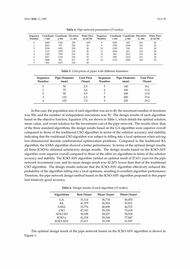
Table 4. Pipe network parameters (15 nodes).

SequenceNumber

Coordinatex (m)

Coordinatey (m)

ElevationGi (m)

Water FlowQ (m3/h)

SequenceNumber

Coordinatex (m)

Coordinatey (m)

ElevationGi (m)

Water FlowQ (m3/h)

0 2085 1320 250 −295 8 2259 925 216 201 2681 377 220 20 9 1785 1098 216 202 2339 1652 220 20 10 1329 769 215 203 1121 1250 219 20 11 2018 421 214 204 1435 1359 219 25 12 562 2213 214 205 2071 1143 218 25 13 898 1212 212 206 2408 851 217 25 14 1314 2020 210 207 964 1637 216 20

Table 5. Unit prices of pipes with different diameters.

SequenceNumber

Pipe Diameter(mm)

Unit Price(Yuan)

SequenceNumber

Pipe Diameter(mm)

Unit Price(Yuan)

0 50 2.5 5 140 8.61 75 3.6 6 160 11.02 90 4.5 7 180 13.03 110 6.2 8 200 15.64 125 7.0 9 225 19.2

In this case, the population size of each algorithm was set to 40, the maximum number of iterationswas 500, and the number of independent executions was 50. The design results of each algorithmbased on the objective function, Equation (19), are shown in Table 6, which details the optimal solution,mean value, and worst solution for the investment cost of the pipe network. The results show that,of the three standard algorithms, the design results based on the GA algorithm were superior overallcompared to those of the traditional CSO algorithm in terms of the solution accuracy and stability,indicating that the traditional CSO algorithm was subject to falling into a local optimum when solvinglow-dimensional discrete combinatorial optimization problems. Compared to the traditional BAalgorithm, the SABA algorithm showed a better performance. In terms of the optimal design results,all three ICSOAs obtained satisfactory design results. The design results based on the ICSO-ASValgorithm were superior overall compared to those of the other six algorithms in terms of the solutionaccuracy and stability. The ICSO-ASV algorithm yielded an optimal result of 27,611 yuan for the pipenetwork investment cost, and its mean design result was 42.20% lower than that of the traditionalCSO algorithm. The design results indicate that the ICSO-ASV algorithm effectively reduced theprobability of the algorithm falling into a local optimum, resulting in excellent algorithm performance.Therefore, the pipe network design method based on the ICSO-ASV algorithm proposed in this paperhad relatively good accuracy.

Table 6. Design results of each algorithm (15 nodes).

Algorithms Best (Yuan) Mean (Yuan) Worst (Yuan)

GA 31,114 36,734 46,053BA 41,379 56,954 93,831

SABA 33,776 40,698 46,572CSO 47,767 59,330 75,018

ADLCSO 30,109 38,227 50,528ICSO-a 41,018 59,344 77,847

ICSO-ASV 27,611 32,338 41,937

The optimal design result of the pipe network based on the ICSO-ASV algorithm is shown inFigure 4.

Water 2020, 12, 1985 15 of 18

Water 2020, 12, x FOR PEER REVIEW 16 of 20

Table 6. Design results of each algorithm (15 nodes).

Algorithms Best (Yuan) Mean (Yuan) Worst (Yuan)

GA 31,114 36,734 46,053

BA 41,379 56,954 93,831

SABA 33,776 40,698 46,572

CSO 47,767 59,330 75,018

ADLCSO 30,109 38,227 50,528

ICSO-a 41,018 59,344 77,847

ICSO-ASV 27,611 32,338 41,937

0

12

65 34

9 8

11

7

12

14

10

13

Water source node

Water node

[ ] Pipe diameter (mm)

[90][90]

[90]

[90]

[90]

[75]

[75]

[75]

[75] [75]

[75]

[75]

[75]

[75]

Figure 4. Optimal design result of the pipe network based on the ICSO-ASV algorithm (15 nodes).

4.3. Pipe Network Design Case II

With the expansion of the scale of the pipe network, that is, with an increase in the number of pipe network nodes, the solution space of the improved pipe network planning model increased exponentially and the difficulty of searching for the optimal solution of the model correspondingly increased. To further verify the scalability of the proposed design method, the second case investigated in this paper, pipe network design case II, included one water source point and 39 water-consuming nodes; the parameters of each node are shown in Table 7.

Figure 4. Optimal design result of the pipe network based on the ICSO-ASV algorithm (15 nodes).

4.3. Pipe Network Design Case II

With the expansion of the scale of the pipe network, that is, with an increase in the number ofpipe network nodes, the solution space of the improved pipe network planning model increasedexponentially and the difficulty of searching for the optimal solution of the model correspondinglyincreased. To further verify the scalability of the proposed design method, the second case investigatedin this paper, pipe network design case II, included one water source point and 39 water-consumingnodes; the parameters of each node are shown in Table 7.

Table 7. Pipe network parameters (40 nodes).

SequenceNumber

Coordinatex (m)

Coordinatey (m)

ElevationGi (m)

Water FlowQ (m3/h)

SequenceNumber

Coordinatex (m)

Coordinatey (m)

ElevationGi (m)

Water FlowQ (m3/h)

0 2085 1320 250 −930 20 2184 521 224 251 1810 1470 238 30 21 1904 816 223 252 2586 1510 237 30 22 575 734 223 203 1535 431 236 25 23 2420 1150 221 254 2210 1165 235 30 24 611 1335 221 255 1570 689 235 25 25 1363 1511 221 256 2681 1570 235 30 26 2681 377 220 207 1727 920 234 20 27 2339 1652 220 208 427 1765 234 25 28 1121 1250 219 209 1738 1526 233 30 29 1435 1359 219 25

10 1649 1389 232 30 30 2071 1143 218 2511 1906 899 231 25 31 2408 851 217 2512 373 1209 231 25 32 964 1637 216 2013 976 1455 230 25 33 2259 925 216 2014 1321 1169 228 25 34 1785 1098 216 2015 1008 725 227 25 35 1329 769 215 2016 2190 1031 227 20 36 2018 421 214 2017 1230 1373 226 20 37 562 2213 214 2018 870 1922 225 20 38 898 1212 212 2019 1411 1703 225 30 39 1314 2020 210 20

The results of the pipe network design based on each algorithm are shown in Table 8. According tothe result analysis, the design result based on the traditional CSO algorithm was superior to that basedon the GA algorithm, indicating that the CSO algorithm had certain advantages over the GA algorithmwhen solving high-dimensional optimization problems. Compared to the traditional BA algorithm,the SABA algorithm could still obtain better design results. Compared to the control algorithms,

Water 2020, 12, 1985 16 of 18

the pipe network design based on the ICSO-ASV algorithm could still obtain relatively more stableoptimal results. The ICSO-ASV algorithm yielded an optimal solution of 127,410 yuan as the pipenetwork investment cost, and its mean design result was 31.09% lower than that of the traditional CSOalgorithm. Therefore, the pipe network design method based on the ICSO-ASV algorithm proposed inthis paper had good scalability. To further improve the practicality of this pipe network design method,we designed a software system to enable the intelligent design of tree-type irrigation pipe networks(See details in Supplementary Materials). After entering the node parameters of the pipe network andsetting the relevant algorithm parameters, the system automatically completes the pipe network designprocess and outputs the results. The 2D and 3D results that were given by the ICSO-ASV algorithm forpipe network design case II are shown in Figures 5 and 6, respectively.

Table 8. Design results of each algorithm (40 nodes).

Algorithms Best (Yuan) Mean (Yuan) Worst (Yuan)

GA 174,720 2,144,100 9,183,900BA 210,540 253,180 325,060

SABA 146,910 175,000 195,800CSO 184,880 218,500 278,870

ADLCSO 161,030 237,440 418,740ICSO 186,860 226,730 268,130

ICSO-ASV 127,410 160,900 200,550Water 2020, 12, x FOR PEER REVIEW 18 of 20

0Water source node

Water node

[ ] Pipe diameter (mm)

89

19

12 13

22 24

3837

25

10

18

32

39

29

17

14

28

35

15

1

4

23

27

2

31

16

26

11

21

3

36

5

7

20

6

3334

30

[140][125]

[125] [180]

[75] [90]

[110]

[125][140]

[140]

[125][160] [140]

[125]

[225]

[110]

[125]

[140]

[90] [75]

[90] [140]

[140]

[125]

[125]

[125][125]

[110]

[75]

[110]

[125]

[125]

[125]

[90]

[140]

[140]

[140]

[75]

[110]

Figure 5. Optimal design results for the pipe network based on the ICSO-ASV algorithm (40 nodes, 2D).

Figure 6. Optimal design results for the pipe network based on the ICSO-ASV algorithm (40 nodes, 3D). Different colors represent different pipe diameters, as shown in the key.

5. Conclusions

This paper proposed an improved planning model for tree-type irrigation pipe networks and verified the effectiveness of the pipe network design method based on the ICSO-ASV algorithm using two pipe network cases with different topologies. The results indicated that the improved pipe network planning model could ensure the pipe connectivity of tree-type irrigation pipe networks via different combinations of water-consuming nodes and upper water nodes. The use of a preliminary connection diagram of the pipe network was not required, and the developed model had relatively good versatility and scalability.

A test function experiment demonstrated that the ICSO-ASV algorithm based on the improved control coefficient pair and adaptive mutation factors had a better global search ability and optimal solution accuracy than the control algorithms. The two pipe network test cases demonstrated that the pipe network design method based on the ICSO-ASV algorithm could effectively reduce the investment cost of a pipe network, and therefore has better practicability than the control algorithms.

This image cannot currently be displayed.

Figure 5. Optimal design results for the pipe network based on the ICSO-ASV algorithm (40 nodes, 2D).

1

Figure 6. Optimal design results for the pipe network based on the ICSO-ASV algorithm (40 nodes, 3D). Different colors represent different pipe diameters, as shown in the key.

Figure 6. Optimal design results for the pipe network based on the ICSO-ASV algorithm (40 nodes, 3D).Different colors represent different pipe diameters, as shown in the key.

Water 2020, 12, 1985 17 of 18

5. Conclusions

This paper proposed an improved planning model for tree-type irrigation pipe networks andverified the effectiveness of the pipe network design method based on the ICSO-ASV algorithm usingtwo pipe network cases with different topologies. The results indicated that the improved pipe networkplanning model could ensure the pipe connectivity of tree-type irrigation pipe networks via differentcombinations of water-consuming nodes and upper water nodes. The use of a preliminary connectiondiagram of the pipe network was not required, and the developed model had relatively good versatilityand scalability.

A test function experiment demonstrated that the ICSO-ASV algorithm based on the improvedcontrol coefficient pair and adaptive mutation factors had a better global search ability and optimalsolution accuracy than the control algorithms. The two pipe network test cases demonstrated that thepipe network design method based on the ICSO-ASV algorithm could effectively reduce the investmentcost of a pipe network, and therefore has better practicability than the control algorithms.

The planning and design problem of tree-type irrigation pipe networks is relatively complex,making it difficult to describe the variability of a network with a single model. In future studies,the instructive research on the optimal design of irrigation pipe networks is as follows: (1) In thedesign process of irrigation pipe networks, the minimization of investment cost should not be theonly issue that designers need to consider; the other issues that also need to be considered, includeterrain conditions, operation management, and reliability. (2) To enhance the computational efficiencyand accuracy, other new swarm intelligence optimization algorithms will be explored in the field ofirrigation pipe network optimization.

Supplementary Materials: The following are available online at http://www.mdpi.com/2073-4441/12/7/1985/s1,DEMO—Optimal design method using ICSO-ASV algorithm.

Author Contributions: Data curation, Z.W. and H.H.; formal analysis, S.L.; funding acquisition, Z.L. (Zhen Li);methodology, Z.L. (Zhen Li) and S.L.; writing—original draft, Z.L. (Zijian Lin). All authors have read and agreedto the published version of the manuscript.

Funding: This work was supported by the National Natural Science Foundation of China (No. 61601189 andNo. 31971797), the Special Fund of Modern Technology System of Agricultural Industry (No. CARS-26), the Scienceand Technology Program of Guangzhou (No. 201803020037), and the Special Fund Support Project for GuangdongUniversity Students (No. pdjh2020a0083).

Conflicts of Interest: The authors declare that there is no conflict of interests regarding the publication ofthis article.

References

1. Alexiou, D.; Tsouros, C. Design of an irrigation network system in terms of canal capacity using graph theory.J. Irrig. Drain. Eng. 2017, 143, 06017002. [CrossRef]

2. Bai, D. Optimal Design of Water Transmission Conduits and Water Distribution Network. Ph.D. Thesis,Xi’an University of Technology, Xi’an, China, 2003.

3. Ma, X.Y.; Fan, X.Y.; Zhao, W.J.; Kang, Y.H. Tree-type pipe network optimization design method based oninteger coding genetic algorithm. J. Hydraul. Eng. 2008, 39, 373–379.

4. Hu, J.H.; Ma, X.Y.; Yao, W.W.; Wang, Z.; Yin, J.C. The design of irrigation networks based on KruskalAlgorithm. China Rural Water Hydropower 2012, 2, 1–3.

5. Lin, X.C.; Zhang, X.P. The optimal designing principle and method for gravititional low pressured pipeirrigation using the orthogonal scheme. J. Irrig. Drain. 1993, 4, 25–29.

6. Wei, Y.Y. Using differential method to calculate the economic diameter of each pipe section of tree-type pipenetwork. Water Sav. Irrig. 1983, 3, 38–42, 60.

7. Wang, X.K.; Cheng, D.L.; Lin, X.C. Optimum design of main pipe net for single well. Trans. Chin. Soc.Agric. Eng. 2001, 3, 41–44.

8. Design and Optimization of Irrigation Pipe Networks. FAO Irrigation and Drainage Collection 44, 2nd ed.;China Agricultural Science and Technology Press: Beijing, China, 1992.

Water 2020, 12, 1985 18 of 18

9. Alomari, A.; Phillips, W.; Aslam, N.; Comeau, F. Swarm intelligence optimization techniques forobstacle-avoidance mobility-assisted localization in wireless sensor networks. IEEE Access 2018, 6,22368–22385. [CrossRef]

10. Li, H.B.; Ma, X.Y.; Zhao, W.J.; Sun, X.J. Layout and diameter simultaneous optimization method of tree pipenetwork. J. Syst. Simul. 2009, 11, 3180–3183.

11. Zhou, R.M.; Lei, Y.F. Optimal layout of tree pipe networks based on improved single parent genetic algorithm.J. Hydraul. Eng. 2012, 43, 1243–1247.

12. Ma, P.H.; Li, Y.N.; Hu, Y.J.; Cui, K.; Qu, Q. Optimal design of gravity tree-type pipe network based onHarmony Search Algorithm. China Rural Water Hydropower 2016, 6, 14–18.

13. Chen, J.X.; Xu, S.Q.; Zhou, H. Optimal design of drip irrigation pipe network using the Firefly Algorithm.J. Irrig. Drain. 2018, 37, 48–55.

14. Meng, X.B.; Liu, Y.; Gao, X.Z.; Zhang, H.Z. A New Bio-Inspired Algorithm: Chicken Swarm Optimization,International Conference in Swarm Intelligence; Springer: Cham, Switzerland, 2014; pp. 86–94.

15. Qu, C.W.; Zhao, S.A.; Fu, Y.M.; He, W. Chicken swarm optimization based on elite opposition-based learning.Math. Probl. Eng. 2017, 2017. [CrossRef]

16. Li, Y.C.; Wang, S.W.; Han, M.X. Truss Structure Optimization Based on Improved Chicken Swarm OptimizationAlgorithm. Adv. Civ. Eng. 2019, 2019. [CrossRef]

17. Wang, J.Q.; Cheng, Z.W.; Ersoy, O.K.; Zhang, M.X.; Sun, K.X.; Bi, Y.S. Improvement and application ofchicken swarm optimization for constrained optimization. IEEE Access 2019, 7, 58053–58072. [CrossRef]

18. Gu, Y.C.; Lu, H.Y.; Xiang, L.; Shen, W.Q. Adaptive dynamic learning chicken swarm optimization algorithm.Comput. Eng. Appl. 2020, 1–12. [CrossRef]

19. Sun, G.; Zhao, X.H.; Liang, S.; Liu, Y.H.; Zhou, X.; Zhang, Y. A modified chicken swarm optimizationalgorithm for synthesizing linear, circular and random antenna arrays. In Proceedings of the 2019 IEEE 90thVehicular Technology Conference (VTC2019-Fall), Honolulu, HI, USA, 22–25 September 2019; pp. 1–7.

20. Fu, C.; Li, G.Q.; Lin, K.P.; Zhang, H.J. Short-term wind power prediction based on improved chickenalgorithm optimization support vector machine. Sustainability 2019, 11, 512. [CrossRef]

21. Niu, P.F.; Ding, X.; Liu, N.; Chang, L.F.; Zhang, X.C. Prediction of boiler NOx emission based on mixedchicken swarm algorithm and kernel extreme learning. Acta Metrol. Sin. 2019, 40, 929–936.

22. Li, P.; Chen, G.F.; Hu, W.T. Research on wireless sensor network location based on chicken swarm optimization.Chin. J. Sens. Actuators 2019, 32, 866–871, 891.

23. Lyu, S.L.; Wu, B.L.; Li, Z.; Hong, T.S.; Wang, J.H.; Huang, Y.L. Tree-Type irrigation pipe network planningusing an improved bat algorithm. Trans. ASABE 2019, 62, 447–459. [CrossRef]

24. Kennedy, J.; Eberhart, R. Particle swarm optimization. In Proceedings of the ICNN’95-InternationalConference on Neural Networks, Perth, Australia, 27 November–1 December 1995; Volume 4, pp. 1942–1948.

25. Yang, X. A new metaheuristic bat-inspired algorithm. In Nature Inspired Cooperative Strategies for Optimization(NICSO 2010), 2nd ed.; Springer: Berlin/Heidelberg, Germany, 2010; pp. 65–74.

26. Robinson, J.; Rahmat-Samii, Y. Particle swarm optimization in electromagnetics. IEEE Trans. Antennas Propag.2004, 52, 397–407. [CrossRef]

27. Damousis, I.G.; Bakirtzis, A.G.; Dokopoulos, P.S. Network-constrained economic dispatch using real-codedgenetic algorithm. IEEE Trans. Power Syst. 2003, 18, 198–205. [CrossRef]

28. Lyu, S.L.; Huang, Y.L.; Chen, H.Q.; Li, Z.; Wang, W.X. Improved bat algorithm using self-adaptive step.Control Decis. 2018, 33, 557–564.

© 2020 by the authors. Licensee MDPI, Basel, Switzerland. This article is an open accessarticle distributed under the terms and conditions of the Creative Commons Attribution(CC BY) license (http://creativecommons.org/licenses/by/4.0/).