tree and network analysis and...
TRANSCRIPT

Tree and Network Analysis and Visualization
Dr. Katy Börner Cyberinfrastructure for Network Science Center, DirectorInformation Visualization Laboratory, DirectorSchool of Library and Information ScienceIndiana University, Bloomington, INhttp://info.slis.indiana.edu/~katy
With special thanks to Kevin W. Boyack, Micah Linnemeier, Russell J. Duhon, Patrick Phillips, Joseph Biberstine, Chintan TankNianli Ma, Hanning Guo, Mark A. Price, Angela M. Zoss, andScott Weingart
Guest Lecture in S604/S764 Information Networks by Staša MilojevićNovember 14, 2011
1. Science of Science Research 2. Information Visualization 3. CIShell Powered Tools: Network Workbench and Science of Science Tool
4. Temporal Analysis—Burst Detection5. Geospatial Analysis and Mapping6. Topical Analysis & Mapping
7. Tree Analysis and Visualization8. Network Analysis9. Large Network Analysis
10. Using the Scholarly Database at IU11. VIVO National Researcher Networking 12. Future Developments
12 Tutorials in 12 Days at NIH—Overview
2
1st Week
2nd Week
3rd Week
4th Week

[#07] Tree Analysis and Visualization General Overview
Designing Effective Tree Visualizations
Notions and Notations
Sci2-Reading and Extracting Trees
Sci2-Visualizing Trees
Outlook
3
Sample Trees and Visualization Goals & Objectives
Goals & Objectives
Representing hierarchical data Structural information Content information
Objectives Efficient Space Utilization Interactivity Comprehension Esthetics
Pat Hanrahan, Stanford Uhttp://www-graphics.stanford.edu/~hanrahan/talks/todrawatree/
4
Sample Trees
Hierarchies File systems and web sites Organization charts Categorical classifications Similarity and clustering
Branching Processes Genealogy and lineages Phylogenetic trees
Decision Processes Indices or search trees Decision trees

Radial Tree – How does it work?See also http://iv.slis.indiana.edu/sw/radialtree.html
All nodes lie in concentric circles that are focused in the center of the screen.
Nodes are evenly distributed.
Branches of the tree do not overlap.
Greg Book & Neeta Keshary (2001) Radial Tree Graph Drawing Algorithm for Representing Large
Hierarchies. University of Connecticut Class Project.
5
Radial Tree – Pseudo Algorithm
Circle PlacementMaximum size of the circle corresponds to minimum screen width or height.Distance between levels d := radius of max circle size / number of levels in the graph.
Node PlacementLevel 0The root node is placed at the center.Level 1All nodes are children of the root node and can be placed over all the 360o of the circle - divide 2pi by the number of nodes at level 1 to get angle space between the nodes on the circle.
6
Radial Tree – Pseudo Algorithm cont.
Levels 2 and greaterUse information on number of parents, their location, and their space for children to place all level x nodes.
Loop through the list of parents and then loop through all the children for that parent and calculate the child’s location relative to the parent’s, adding in the offset of the limit angle.
After calculating the location, if there are any directories at the level, we must calculate the bisector and tangent limits for those directories.
7
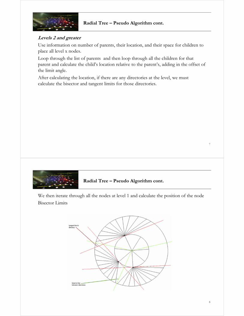
Radial Tree – Pseudo Algorithm cont.
We then iterate through all the nodes at level 1 and calculate the position of the node
Bisector Limits
8
Radial Tree – Pseudo Algorithm cont.
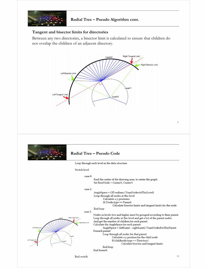
Tangent and bisector limits for directories
Between any two directories, a bisector limit is calculated to ensure that children do not overlap the children of an adjacent directory.
9
Radial Tree – Pseudo Code
10

Hyperbolic Tree – How does it work?See also http://sw.slis.indiana.edu/sw/hyptree.html
11
Phylogenetic Tree
Hyperbolic Geometry
Inspired by Escher’s Circle Limit IV (Heaven and Hell), 1960.
Focus+context technique for visualizing large hierarchies
Continuous redirection of the focus possible.
The hyperbolic plane is a non-Euclidean geometry in which parallel lines diverge away
from each other. This leads to the convenient property that the circumference of a
circle on the hyperbolic plane grows exponentially with its radius, which means that
exponentially more space is available with increasing distance.
J. Lamping, R. Rao, and P. Pirolli (1995) A focus+context technique based on hyperbolic geometry for
visualizing large hierarchies. Proceedings of the ACM CHI '95 Conference - Human Factors in Computing
Systems, 1995, pp. 401-408.
12
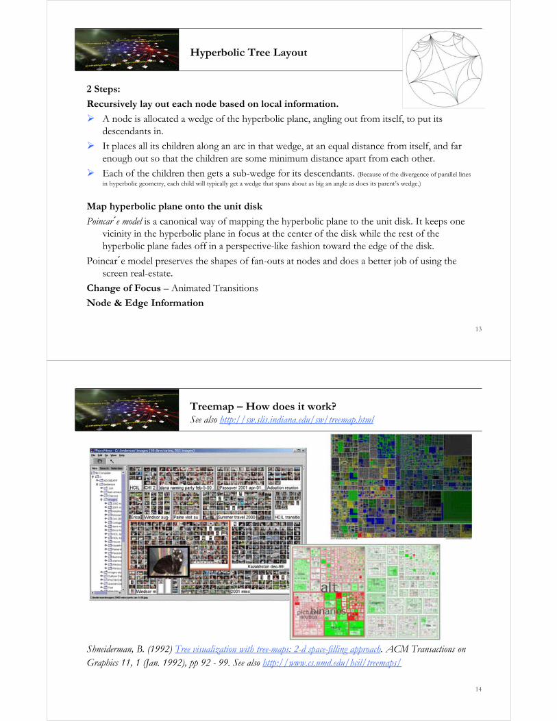
Hyperbolic Tree Layout
2 Steps:
Recursively lay out each node based on local information.
A node is allocated a wedge of the hyperbolic plane, angling out from itself, to put its descendants in.
It places all its children along an arc in that wedge, at an equal distance from itself, and far enough out so that the children are some minimum distance apart from each other.
Each of the children then gets a sub-wedge for its descendants. (Because of the divergence of parallel lines in hyperbolic geometry, each child will typically get a wedge that spans about as big an angle as does its parent’s wedge.)
Map hyperbolic plane onto the unit disk
Poincar´e model is a canonical way of mapping the hyperbolic plane to the unit disk. It keeps one vicinity in the hyperbolic plane in focus at the center of the disk while the rest of the hyperbolic plane fades off in a perspective-like fashion toward the edge of the disk.
Poincar´e model preserves the shapes of fan-outs at nodes and does a better job of using the screen real-estate.
Change of Focus – Animated Transitions
Node & Edge Information
13
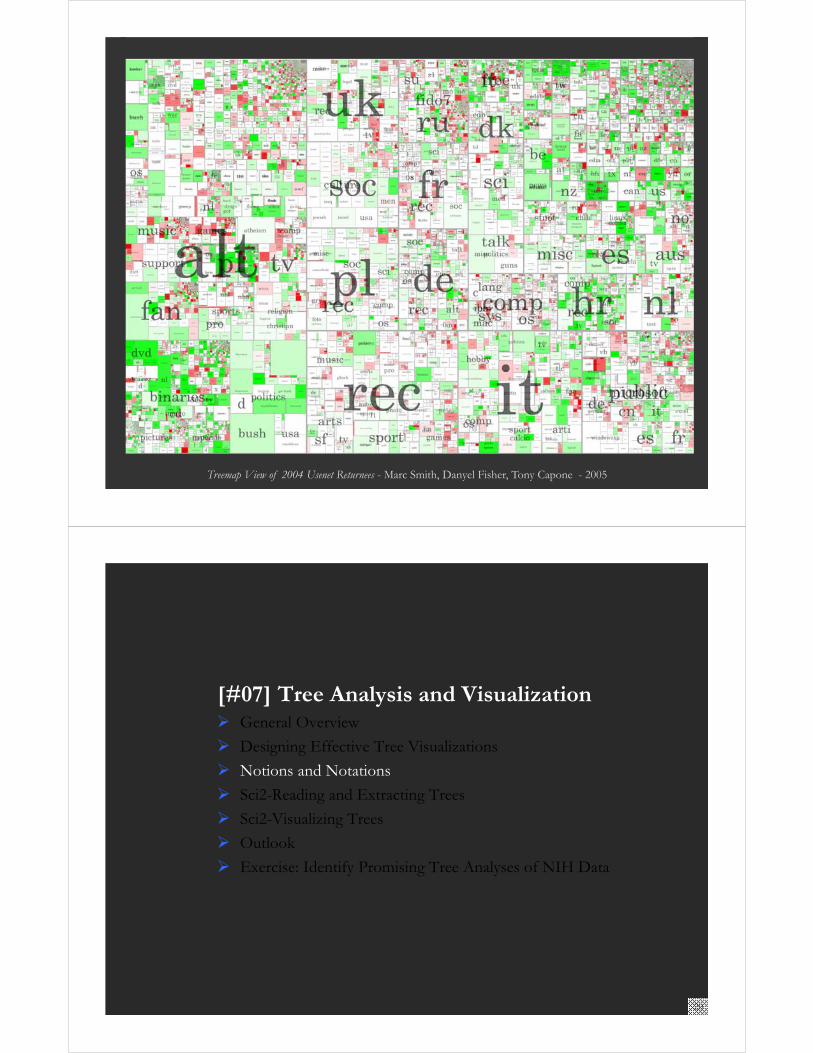
Treemap – How does it work?See also http://sw.slis.indiana.edu/sw/treemap.html
Shneiderman, B. (1992) Tree visualization with tree-maps: 2-d space-filling approach. ACM Transactions on Graphics 11, 1 (Jan. 1992), pp 92 - 99. See also http://www.cs.umd.edu/hcil/treemaps/
14

Treemaps – Layout
Ben Shneiderman, Tree Visualization with Tree-Maps: 2-d Space-Filling Approach
size
15
Treemap – Pseudo Code
Input
Tree root & a rectangular area defined by upper left and lower right
coordinates Pl(xl, yl), Q1(x2, y2).
Recursive Algorithm
active_node := root_node;
partitioning_direction := horizontal; // nodes are partitioned vertically at even levels and horizontally at odd levels
Tremap(active_node) {
determine number n of outgoing edges from the active_node;
if (n<1)
end;
if (n>1) {
divide the region [xl, x2] in partitioning_direction were the size of
the n partitions correspond to their fraction
(Size(child[i])/Size(active)) of the total number of bytes
in the active_node;
change partitioning_direction;
for (1<=i<=n) do
Treemap(child[i]);
}
16

Treemap – Properties
Strengths
Utilizes 100% of display space
Shows nesting of hierarchical levels.
Represents node attributes (e.g., size and age) by area size and color
Scalable to data sets of a million items.
Weaknesses
Size comparison is difficult
Labeling is a problem.
Cluttered display
Difficult to discern boundaries
Shows only leaf content information
17
Treemap – Algorithm Improvements
Sorted treemap Cushion treemap
Marc Smith http://treemap.sourceforge.net/
18
Treemap View of 2004 Usenet Returnees - Marc Smith, Danyel Fisher, Tony Capone - 2005
[#07] Tree Analysis and Visualization General Overview
Designing Effective Tree Visualizations
Notions and Notations
Sci2-Reading and Extracting Trees
Sci2-Visualizing Trees
Outlook
Exercise: Identify Promising Tree Analyses of NIH Data
20

Tree Nodes and Edges
The root node of a tree is the node with no parents.
A leaf node has no children.
In-degree of a node is the number of edges arriving at that node.
Out-degree of a node is the number of edges leaving that node.
Sample tree of
size 11 (=number of nodes) and height 4 (=number of levels).
designated root node
parent of A
sibling of A
child of A
leaf nodes
Aleaf nodes
21
1
2
3
4
[#07] Tree Analysis and Visualization General Overview
Designing Effective Tree Visualizations
Notions and Notations
Sci2-Reading and Extracting Trees
Sci2-Visualizing Trees
Outlook
Exercise: Identify Promising Tree Analyses of NIH Data
22
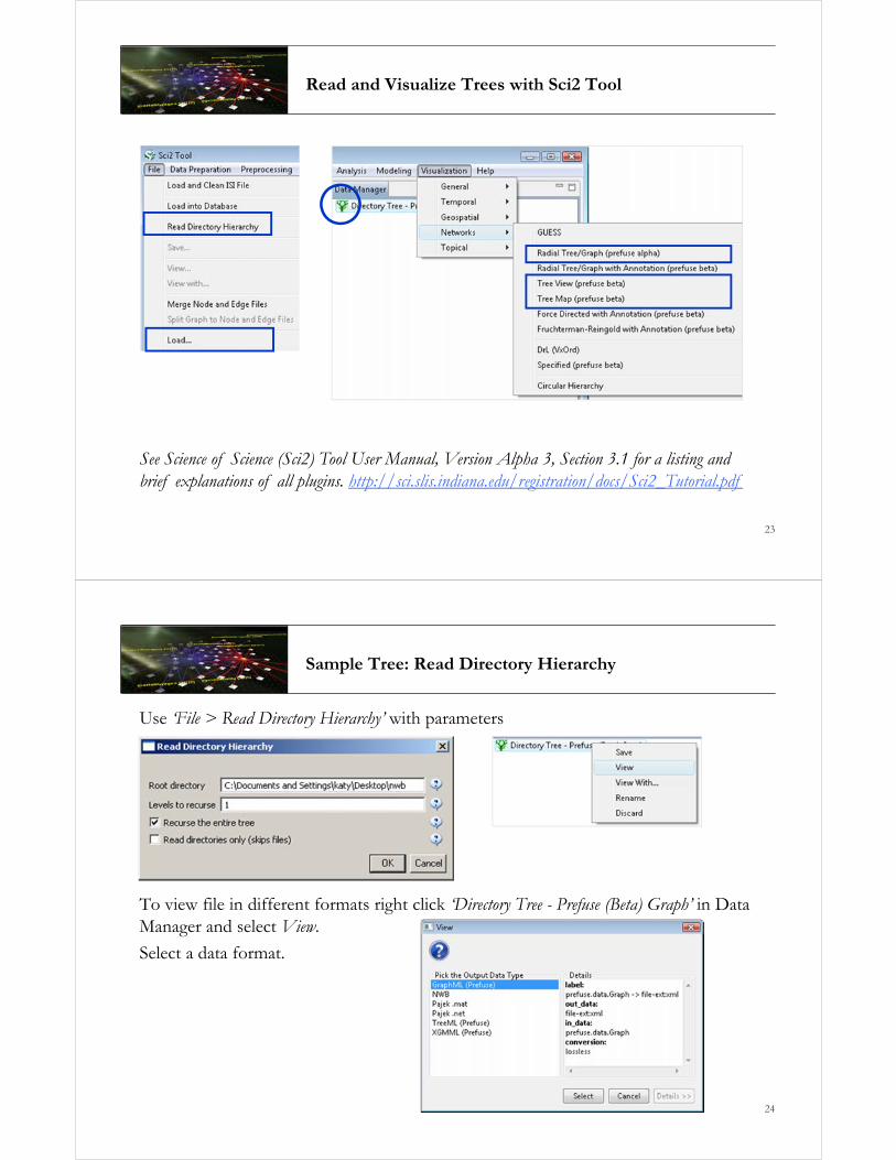
Read and Visualize Trees with Sci2 Tool
23
See Science of Science (Sci2) Tool User Manual, Version Alpha 3, Section 3.1 for a listing and brief explanations of all plugins. http://sci.slis.indiana.edu/registration/docs/Sci2_Tutorial.pdf
Sample Tree: Read Directory Hierarchy
Use ‘File > Read Directory Hierarchy’ with parameters
To view file in different formats right click ‘Directory Tree - Prefuse (Beta) Graph’ in Data Manager and select View.
Select a data format.
24
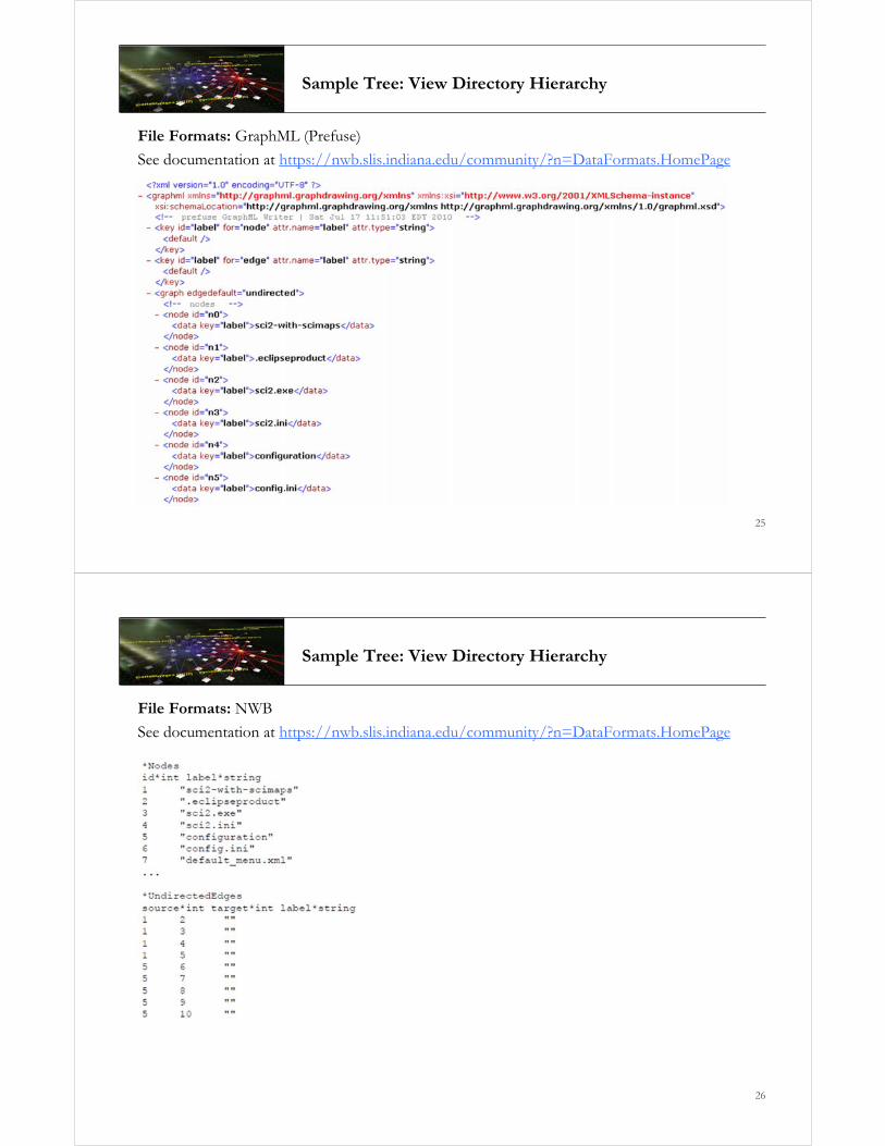
Sample Tree: View Directory Hierarchy
File Formats: GraphML (Prefuse)
See documentation at https://nwb.slis.indiana.edu/community/?n=DataFormats.HomePage
25
Sample Tree: View Directory Hierarchy
File Formats: NWB
See documentation at https://nwb.slis.indiana.edu/community/?n=DataFormats.HomePage
26

Sample Tree: View Directory Hierarchy
File Formats: Pajek .net Note similarity to .nwbSee documentation athttps://nwb.slis.indiana.edu/community/?n=DataFormats.HomePage
27
Sample Tree: View Directory Hierarchy
File Formats: Pajek .matSee documentation at https://nwb.slis.indiana.edu/community/?n=DataFormats.HomePage
…
28
29
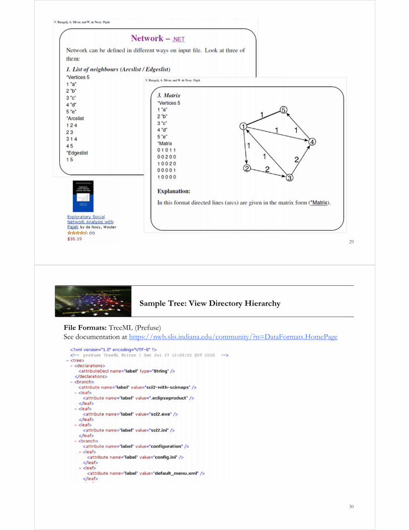
Sample Tree: View Directory Hierarchy
File Formats: TreeML (Prefuse)See documentation at https://nwb.slis.indiana.edu/community/?n=DataFormats.HomePage
30
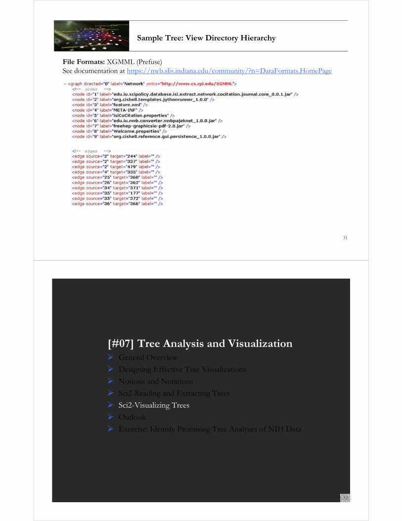
Sample Tree: View Directory Hierarchy
File Formats: XGMML (Prefuse)See documentation at https://nwb.slis.indiana.edu/community/?n=DataFormats.HomePage
31
[#07] Tree Analysis and Visualization General Overview
Designing Effective Tree Visualizations
Notions and Notations
Sci2-Reading and Extracting Trees
Sci2-Visualizing Trees
Outlook
Exercise: Identify Promising Tree Analyses of NIH Data
32

Sample Tree Visualizations
Indented Lists and Tree View showing nesting of, e.g., directory hierarchies.
Visualize ‘Directory Tree - Prefuse (Beta) Graph’ using
• ‘‘Visualization > Networks > Tree View (prefuse beta)’
Press right mouse button and use mouse wheel/touch pad to zoom in and out.
Click on directory to expand/collapse.
Use search field to find specific files. 33
Sample Tree Visualizations
Radial Tree and Ballon Tree showing the structure of, e.g., directory hierarchies.
Visualize ‘Directory Tree - Prefuse (Beta) Graph’ using
• ‘‘Visualization > Networks > Radial Tree/Graph (prefuse alpha)’
• ‘‘Visualization > Networks > Balloon Graph (prefuse alpha)’ (not in Sci2 Tool, Alpha 3)
34

Sample Tree Visualization
Tree Map showing the structure of, e.g., directory hierarchies.
Visualize ‘Directory Tree - Prefuse (Beta) Graph’ using
• ‘Visualization > Networks > Tree Map (prefuse beta)’
35
Sample Tree Visualization
Flow Maps showing migration patterns
http://graphics.stanford.edu/papers/flow_map_layoutSoon available in Sci2 Tool.
36

[#07] Tree Analysis and Visualization General Overview
Designing Effective Tree Visualizations
Notions and Notations
Sci2-Reading and Extracting Trees
Sci2-Visualizing Trees
Outlook
Exercise: Identify Promising Tree Analyses of NIH Data
37
Outlook
Planned extensions of Sci2 Tool:
(Flowmap) tree network overlays for geo maps and science maps.
Bimodal network visualizations.
Scalable visualizations of large hierarchies.
38
Research Collaborations by the Chinese Academy of SciencesBy Weixia (Bonnie) Huang, Russell J. Duhon, Elisha F. Hardy, Katy Börner, Indiana University, USA
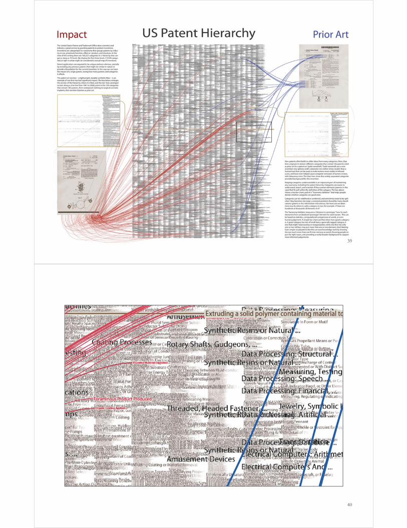
39
40

41
42
[#08] Network Analysis and Visualization General Overview
Designing Effective Network Visualizations
Notions and Notations
Sci2-Reading and Extracting Networks
Sci2-Analysing Networks
Sci2-Visualizing Networks
Outlook
43
Information Visualization Course, Katy Börner, Indiana University
Sample Networks
Communication networks Internet, telephone network, wireless network.
Network applications The World Wide Web, Email interactions
Transportation network/ Road maps Relationships between objects in a data base
Function/module dependency graphs Knowledge bases
Network Properties Directed vs. undirected Weighted vs. unweighted Additional node and edge attributes One vs. multiple node & edge types Network type (random, small world, scale free, hierarchical networks)
44

Co-word space of the top 50 highly frequent and bursty words used in the top 10% most highly cited PNAS publications in 1982-2001.
(Mane & Börner, 2004)
Reducing the number of edges via pathfinder network scaling.
45
Network Visualization, Katy Börner, Indiana University
Historiograph of DNA Development(Garfield, Sher, & Torpie, 1964)
Direct or strongly implied citationIndirect citation
46

Force Directed Layout – How does it work?
The algorithm simulates a system of forces defined on an input graph and outputs a locally minimum energy configuration. Nodes resemble mass points repelling each other and the edges simulate springs with attracting forces. The algorithm tries to minimize the energy of this physical system of mass particles.
Required are
- A force model
- Technique for finding locally
minimum energy configurations.
P. Eades,"A heuristic for graph drawing“
Congressus Numerantium, 42,149-160,1984.
47
Force Directed Layout cont.
Force Models
A simple algorithm to find the equilibrium configuration is to trace the move of each node according to Newton’s 2nd law. This takes time O n3, which makes it unsuitable for large data sets. Rob Forbes (1987) proposed two methods that were able to accelerate convergence of a FDP problem 3-4 times. One stabilizes the derivative of the repulsion force and the other uses information on node movement and instability characteristics to make a predictive extrapolation.
48

Force Directed Layout cont.
Most existing algorithms extend Eades’ algorithm (1984) by providing methods for the intelligent initial placement of nodes, clustering the data to perform an initial coarse layout followed by successively more detailed placement, and grid-based systems for dividing up the dataset.
GEM (Graph EMbedder) attempts to recognize and forestall non-productive rotation and oscillation in the motion of nodes in the graph as it cools, seeFrick, A., A. Ludwig and H. Mehldau (1994). A fast adaptive layout algorithm for undirected graphs. Graph Drawing, Springer-Verlag: 388-403.
Walshaw’s (2000) multilevel algorithm provides a “divide and conquer” method for laying out very large graphs by using clustering, seeWalshaw, C. (2000). A multilevel algorithm for force-directed graph drawing. 8th International Symposium Graph Drawing, Springer-Verlag: 171-182.
49
Force Directed Layout cont.
VxOrd (Davidson, Wylie et al. 2001) uses a density grid in place of pair-wise repulsive forces to speed up execution and achieves computation times order O(N) rather than O(N2). It also employs barrier jumping to avoid trapping of clusters in local minima. Davidson, G. S., B. N. Wylie and K. W. Boyack (2001). "Cluster stability and the use of noise in interpretation of clustering." Proc. IEEE Information Visualization 2001: 23-30.
An extremely fast layout algorithm for visualizing large-scale networks in three-dimensional space was proposed by (Han and Ju 2003). Han, K. and B.-H. Ju (2003). "A fast layout algorithm for protein interaction networks." Bioinformatics19(15): 1882-1888.
Today, the algorithm developed by Kamada and Kawai (Kamada and Kawai 1989) and Fruchterman and Reingold (Fruchterman and Reingold 1991) are most commonly used, partially because they are available in Pajek. Fruchterman, T. M. J. and E. M. Reingold (1991). "Graph Drawing by Force-Directed Placement." Software-Practice & Experience 21(11): 1129-1164.Kamada, T. and S. Kawai (1989). "An algorithm for drawing general undirected graphs." Information Processing Letters 31(1): 7-15.
50
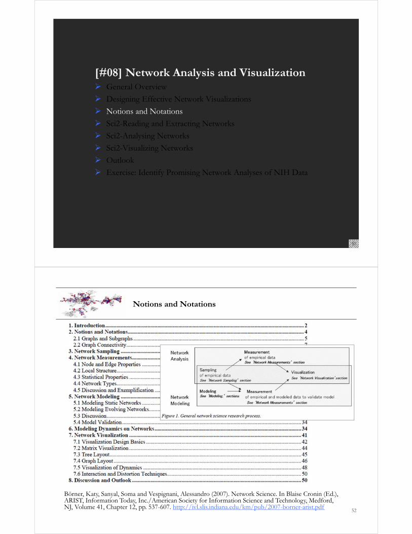
[#08] Network Analysis and Visualization General Overview
Designing Effective Network Visualizations
Notions and Notations
Sci2-Reading and Extracting Networks
Sci2-Analysing Networks
Sci2-Visualizing Networks
Outlook
Exercise: Identify Promising Network Analyses of NIH Data
51
Notions and Notations
52
Börner, Katy, Sanyal, Soma and Vespignani, Alessandro (2007). Network Science. In Blaise Cronin (Ed.), ARIST, Information Today, Inc./American Society for Information Science and Technology, Medford, NJ, Volume 41, Chapter 12, pp. 537-607. http://ivl.slis.indiana.edu/km/pub/2007-borner-arist.pdf

Notions and Notations
53
Börner, Katy, Sanyal, Soma and Vespignani, Alessandro (2007). Network Science. In Blaise Cronin (Ed.), ARIST, Information Today, Inc./American Society for Information Science and Technology, Medford, NJ, Volume 41, Chapter 12, pp. 537-607. http://ivl.slis.indiana.edu/km/pub/2007-borner-arist.pdf
Notions and Notations
54
Börner, Katy, Sanyal, Soma and Vespignani, Alessandro (2007). Network Science. In Blaise Cronin (Ed.), ARIST, Information Today, Inc./American Society for Information Science and Technology, Medford, NJ, Volume 41, Chapter 12, pp. 537-607. http://ivl.slis.indiana.edu/km/pub/2007-borner-arist.pdf

Notions and Notations
55
Börner, Katy, Sanyal, Soma and Vespignani, Alessandro (2007). Network Science. In Blaise Cronin (Ed.), ARIST, Information Today, Inc./American Society for Information Science and Technology, Medford, NJ, Volume 41, Chapter 12, pp. 537-607. http://ivl.slis.indiana.edu/km/pub/2007-borner-arist.pdf
[#08] Network Analysis and Visualization General Overview
Designing Effective Network Visualizations
Notions and Notations
Sci2-Reading and Extracting Networks
Sci2-Analysing Networks
Sci2-Visualizing Networks
Outlook
Exercise: Identify Promising Network Analyses of NIH Data
56

Network Extraction - Examples
Sample paper network (left) and four different network types derived from it (right).From ISI files, about 30 different networks can be extracted.
57
Extract Networks with Sci2 Tool – Database
See Science of Science (Sci2) Tool User Manual, Version Alpha 3, Section 3.1 for a listing and brief explanations of all plugins. http://sci.slis.indiana.edu/registration/docs/Sci2_Tutorial.pdfSee also Tutorial #3
58
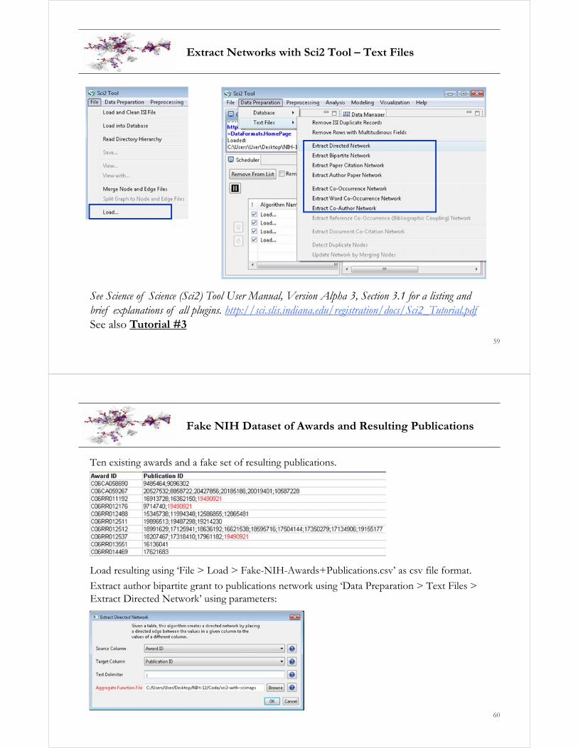
Extract Networks with Sci2 Tool – Text Files
See Science of Science (Sci2) Tool User Manual, Version Alpha 3, Section 3.1 for a listing and brief explanations of all plugins. http://sci.slis.indiana.edu/registration/docs/Sci2_Tutorial.pdfSee also Tutorial #3
59
Fake NIH Dataset of Awards and Resulting Publications
Ten existing awards and a fake set of resulting publications.
Load resulting using ‘File > Load > Fake-NIH-Awards+Publications.csv’ as csv file format.
Extract author bipartite grant to publications network using ‘Data Preparation > Text Files > Extract Directed Network’ using parameters:
60
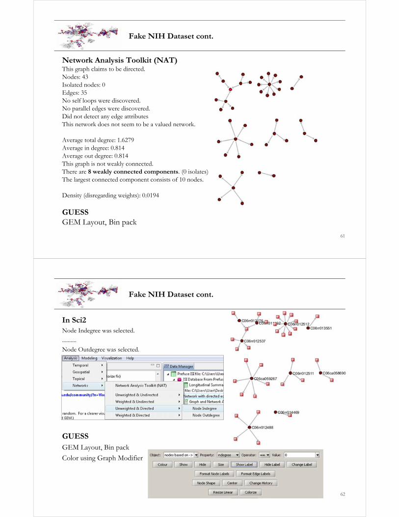
Fake NIH Dataset cont.
Network Analysis Toolkit (NAT)This graph claims to be directed.Nodes: 43Isolated nodes: 0Edges: 35No self loops were discovered.No parallel edges were discovered.Did not detect any edge attributesThis network does not seem to be a valued network.
Average total degree: 1.6279Average in degree: 0.814Average out degree: 0.814This graph is not weakly connected.There are 8 weakly connected components. (0 isolates)The largest connected component consists of 10 nodes.
Density (disregarding weights): 0.0194
GUESSGEM Layout, Bin pack
61
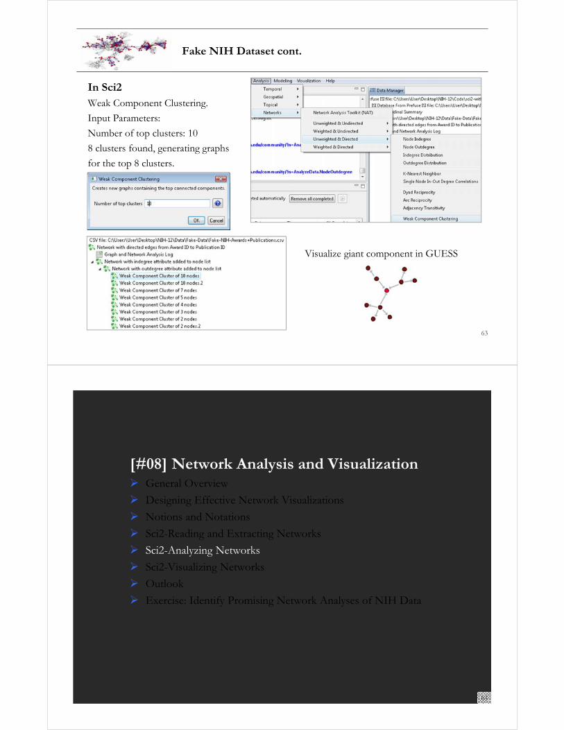
Fake NIH Dataset cont.
In Sci2Node Indegree was selected.
..........
Node Outdegree was selected.
GUESSGEM Layout, Bin pack
Color using Graph Modifier
62
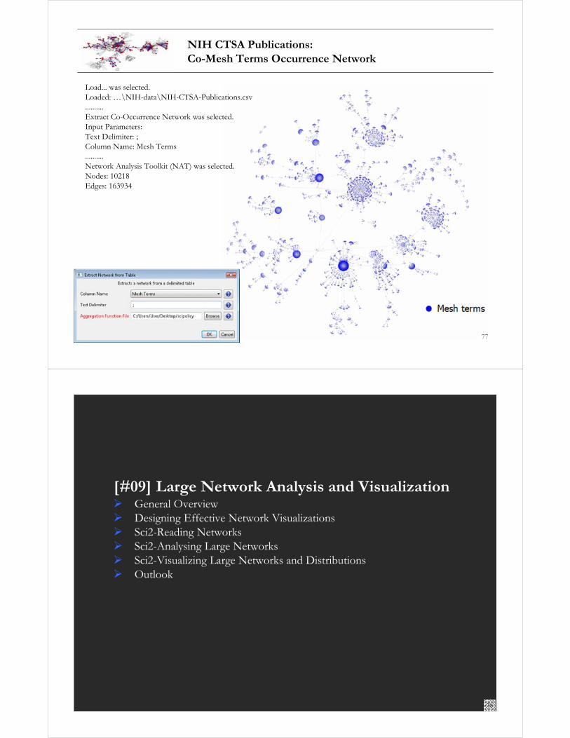
Fake NIH Dataset cont.
In Sci2Weak Component Clustering.
Input Parameters:
Number of top clusters: 10
8 clusters found, generating graphs
for the top 8 clusters.
..........
Visualize giant component in GUESS
63
[#08] Network Analysis and Visualization General Overview
Designing Effective Network Visualizations
Notions and Notations
Sci2-Reading and Extracting Networks
Sci2-Analyzing Networks
Sci2-Visualizing Networks
Outlook
Exercise: Identify Promising Network Analyses of NIH Data
64

Couple Network Analysis and Visualizationto Generate Readable Layouts of Large Graphs
Discover Landmark Nodes based on Connectivity (degree or BC values) Frequency of access(Source: Mukherjea & Hara, 1997; Hearst p. 38 formulas)
Identify Major (and Weak) Links
Identify the Backbone
Show Clusters
See also Ketan Mane’s Qualifying Paper Pajek Tutorialhttp://ella.slis.indiana.edu/~kmane/phdprogress/quals/kmane_quals.pdfhttp://ella.slis.indiana.edu/~katy/teaching/ketan-quals-slides.ppt
65
[#08] Network Analysis and Visualization General Overview
Designing Effective Network Visualizations
Notions and Notations
Sci2-Reading and Extracting Networks
Sci2-Analysing Networks
Sci2-Visualizing Networks
Outlook
Exercise: Identify Promising Network Analyses of NIH Data
66

Network Visualization, Katy Börner, Indiana University
Network Visualization
General Visualization Objectives
Representing structural information & content information
Efficient space utilization
Easy comprehension
Aesthetics
Support of interactive exploration
Challenges in Visualizing Large Networks
Positioning nodes without overlap
De-cluttering links
Labeling
Navigation/interaction
67
General Network Representations
Matrices Structure Plots
Lists of nodes & links Network layouts of nodes and links
Equivalenced representation of US power network
68

Aesthetic Criteria for Network Visualization
Symmetric.
Evenly distributed nodes.
Uniform edge lengths.
Minimized edge crossings.
Orthogonal drawings.
Minimize area / bends / slopes / angles
Optimization criteria may be relaxed to speed up layout process.
(Source: Fruchterman & R. alg p. 76, see Table & discussion Hearst, p 88)
69
Aesthetic Network Visualization
http://www.genome.ad.jp/kegg/pathway/map/map01100.html
70

Small Networks
Up to 100 nodes
All nodes and edges and most of their attributes can be shown.
General mappings for
nodes
# -> (area) size
Intensity (secondary value) -> color
Type -> shape
edges
# -> thickness
Intensity, age, etc. -> color
Type -> style
71
Medium Size Networks
Up to 10,000 nodes
Most nodes can be shown but not all their labels.
Frequently, the number of edges and attributes need to be reduced.
Major design strategies:
Show only important nodes, edges, labels, attributes
Order nodes spatially
Reduce number of displayed nodes
3
72

Visualize Networks with Sci2 Tool
See Science of Science (Sci2) Tool User Manual, Version Alpha 3, Section 3.1 for a listing and brief explanations of all plugins. http://sci.slis.indiana.edu/registration/docs/Sci2_Tutorial.pdf
73
NSF Medical+Health Funding: Bimodal Network of NSF Organization to Program(s)
Extract Directed Network was selected.Source Column: NSF OrganizationText Delimiter: |Target Column: Program(s)
Nodes: 167Isolated nodes: 0Edges: 177No parallel edges were discovered.Did not detect any edge attributesDensity (disregarding weights): 0.00638
IIS
74

Load into NWB, open file to count records, compute total award amount.
Run ‘Scientometrics > Extract Directed Network’ using parameters:
Select “Extracted Network ..” and run ‘Analysis > Network Analysis Toolkit (NAT)’
Remove unconnected nodes via ‘Preprocessing > Delete Isolates’.
Run ‘Analysis > Unweighted & Directed Network > Node Indegree / Node Outdegree’.
‘Visualization > GUESS’ , layout with GEM, Bin Pack Use Graph Modifier to color/size network.
NSF Medical+Health Funding: Extract Principal Investigator: Co-PI Networks
75
NIH CTSA Grants:Co-Project Term Descriptions Occurrence Network
76
Load... was selected.Loaded: …\NIH-data\NIH-CTSA-Grants.csv..........Extract Co-Occurrence Network was selected.Input Parameters:Text Delimiter: ...Column Name: Project term descriptions..........Network Analysis Toolkit (NAT) was selected.Nodes: 5723Isolated nodes: 3Edges: 353218
NIH CTSA Publications:Co-Mesh Terms Occurrence Network
77
Load... was selected.Loaded: …\NIH-data\NIH-CTSA-Publications.csv..........Extract Co-Occurrence Network was selected.Input Parameters:Text Delimiter: ; Column Name: Mesh Terms..........Network Analysis Toolkit (NAT) was selected.Nodes: 10218Edges: 163934
[#09] Large Network Analysis and Visualization General Overview Designing Effective Network Visualizations Sci2-Reading Networks Sci2-Analysing Large Networks Sci2-Visualizing Large Networks and Distributions Outlook
78

Large Networks
More than 10,000 nodes.
Neither all nodes nor all edges can be shown at once. Sometimes, there are more nodes than pixels.
Examples of large networks
Communication networks: Internet, telephone network, wireless network.
Network applications: The World Wide Web, Email interactions
Transportation network/road maps
Relationships between objects in a data base: Function/module dependency graphs
Knowledge bases
79
http://loadrunner.uits.iu.edu/weathermaps/abilene/
Amsterdam RealTime project, WIRED Magazine, Issue 11.03 - March 2003 80
Direct Manipulation
Modify focusing parameters while continuously provide visual feedback and update
display (fast computer response).
Conditioning: filter, set background variables and display foreground parameters
Identification: highlight, color, shape code
Parameter control: line thickness, length, color legend, time slider, and animation control
Navigation: Bird’s Eye view, zoom, and pan
Information requests: Mouse over or click on a node to retrieve more details or collapse/expand a subnetwork
See NIH Awards Viewer at http://scimaps.org/maps/nih/2007/
81
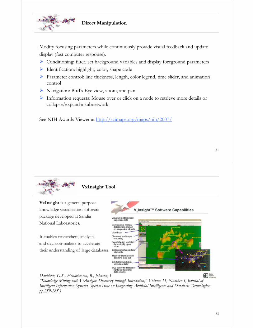
VxInsight Tool
VxInsight is a general purpose
knowledge visualization software
package developed at Sandia
National Laboratories.
It enables researchers, analysts,
and decision-makers to accelerate
their understanding of large databases.
Davidson, G.S., Hendrickson, B., Johnson, D.K., Meyers, C.E., Wylie, B.N., November/December 1998. "Knowledge Mining with VxInsight: Discovery through Interaction," Volume 11, Number 3, Journal of Intelligent Information Systems, Special Issue on Integrating Artificial Intelligence and Database Technologies. pp.259-285.)
82

Other Tools
See http://ivl.slis.indiana.edu/km/pub/2010-borner-et-al-nwb.pdf for references. 83
Other Tools cont.
See http://ivl.slis.indiana.edu/km/pub/2010-borner-et-al-nwb.pdf for references. 84

[#09] Large Network Analysis and Visualization General Overview Designing Effective Network Visualizations Sci2-Reading Networks Sci2-Analyzing Large Networks Sci2-Visualizing Large Networks and Distributions Outlook Exercise: Identify Promising Large Network Analyses of NIH Data
85
Original Data
Extract Network Extract Bipartite Network was selected.
Input Parameters:
First column: Source Node
Text Delimiter: ;
Second column: Target Nodes
Network Analysis and Visualization – General Workflow
86
Calculate Node Attributes
Visualization/Layout

Original Data
Millions of records, in 100s of columns. SAS and Excel might not be able to handle these files.Files are shared between DB and tools as delimited text files (.csv).
Extract Network
It might take several hours to extract a network on a laptop or even on a parallel cluster.
Large Network Analysis & Visualization – General Workflow
87
Derived Statistics
Degree distributionsNumber of components and their sizesExtract giant component, subnetworks for further analysis
Visualizations
It is typically not possible to layout the network.DrL scales to 10 million nodes.
DrL is a force‐directed graph layout toolbox for real‐world large‐scale graphs up to
2 million nodes. It includes:
Standard force‐directed layout of graphs using algorithm based on the popular VxOrdroutine (used in the VxInsight program).
Parallel version of force‐directed layout algorithm.
Recursive multilevel version for obtaining better layouts of very large graphs.
Ability to add new vertices to a previously drawn graph.
The version of DrL included in Sci2 only does the standard force‐directed layout (no
recursive or parallel computation).
Davidson, G. S., B. N. Wylie and K. W. Boyack (2001). "Cluster stability and the use of noise in
interpretation of clustering." Proc. IEEE Information Visualization 2001: 23-30.
DrL Large Network LayoutSee Section 4.9.4.2 in Sci2 Tutorial, http://sci.slis.indiana.edu/registration/docs/Sci2_Tutorial.pdf
88

How to use: DrL expects the edges to be weighted and undirected where the non‐zero
weight denotes how similar the two nodes are (higher is more similar). Parameters are as
follows:
The edge cutting parameter expresses how much automatic edge cutting should be done. 0 means as little as possible, 1 as much as possible. Around .8 is a good value to use.
The weight attribute parameter lets you choose which edge attribute in the network corresponds to the similarity weight. The X and Y parameters let you choose the attribute names to be used in the returned network which corresponds to the X and Y coordinates computed by the layout algorithm for the nodes.
DrL is commonly used to layout large networks, e.g., those derived in co‐citation and
co‐word analyses. In the Sci2 Tool, the results can be viewed in either GUESS or
‘Visualization > Specified (prefuse alpha)’.
See also https://nwb.slis.indiana.edu/community/?n=VisualizeData.DrL
DrL Large Network LayoutSee Section 4.9.4.2 in Sci2 Tutorial, http://sci.slis.indiana.edu/registration/docs/Sci2_Tutorial.pdf
89
Use Ctrl+Alt+Delete to see CPU and Memory Usage


Evolving collaboration networks
93
Evolving collaboration networks
94
Load isi formatted file
As csv, file looks like:
Visualize each time slide separately:

95http://sci2.wiki.cns.iu.edu/5.1.2+Time+Slicing+of+Co-Authorship+Networks+(ISI+Data)
Relevant Sci2 Manual entry
96http://sci2.wiki.cns.iu.edu/5.1.2+Time+Slicing+of+Co-Authorship+Networks+(ISI+Data)
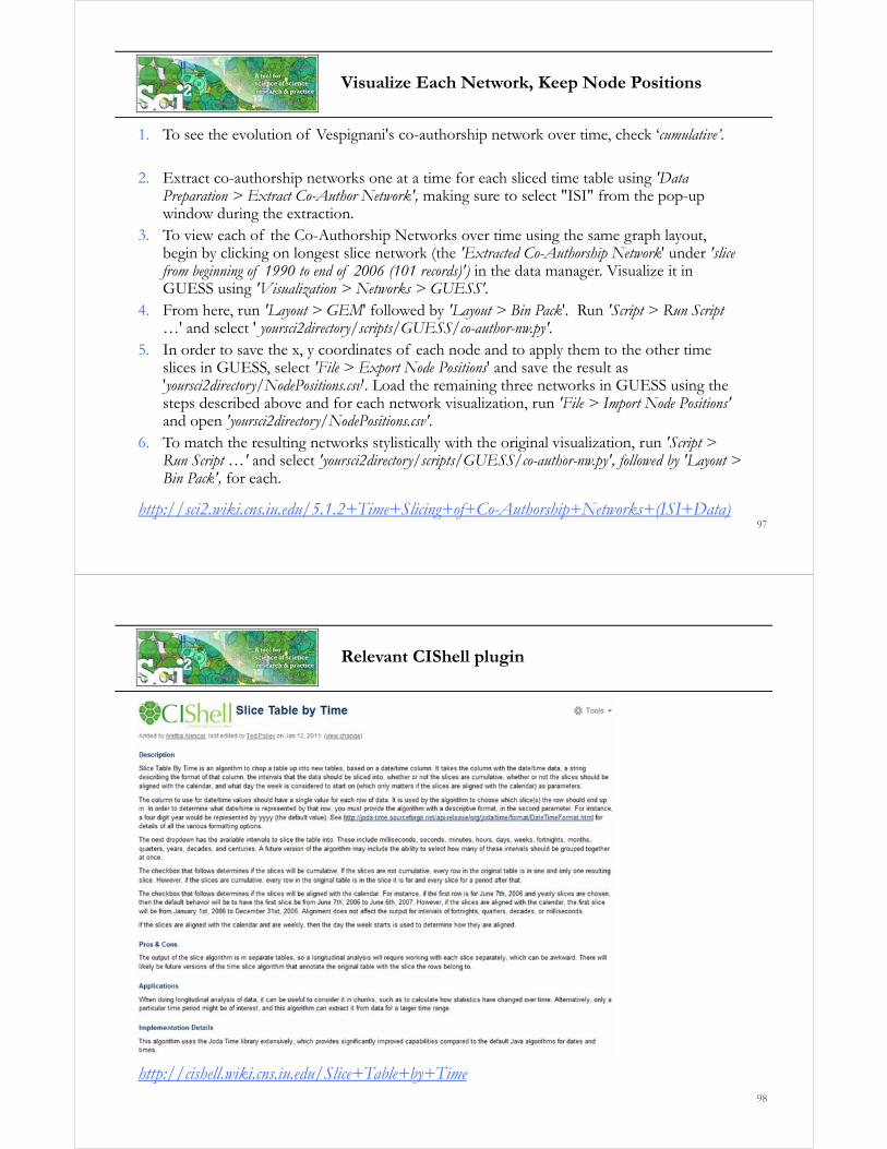
Slice Table by Time
97http://sci2.wiki.cns.iu.edu/5.1.2+Time+Slicing+of+Co-Authorship+Networks+(ISI+Data)
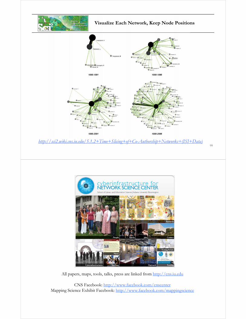
Visualize Each Network, Keep Node Positions
1. To see the evolution of Vespignani's co-authorship network over time, check ‘cumulative’.
2. Extract co-authorship networks one at a time for each sliced time table using 'Data Preparation > Extract Co-Author Network', making sure to select "ISI" from the pop-up window during the extraction.
3. To view each of the Co-Authorship Networks over time using the same graph layout, begin by clicking on longest slice network (the 'Extracted Co-Authorship Network' under 'slice from beginning of 1990 to end of 2006 (101 records)') in the data manager. Visualize it in GUESS using 'Visualization > Networks > GUESS'.
4. From here, run 'Layout > GEM' followed by 'Layout > Bin Pack'. Run 'Script > Run Script…' and select ' yoursci2directory/scripts/GUESS/co-author-nw.py'.
5. In order to save the x, y coordinates of each node and to apply them to the other time slices in GUESS, select 'File > Export Node Positions' and save the result as 'yoursci2directory/NodePositions.csv'. Load the remaining three networks in GUESS using the steps described above and for each network visualization, run 'File > Import Node Positions'and open 'yoursci2directory/NodePositions.csv'.
6. To match the resulting networks stylistically with the original visualization, run 'Script > Run Script …' and select 'yoursci2directory/scripts/GUESS/co-author-nw.py', followed by 'Layout > Bin Pack', for each.
98
http://cishell.wiki.cns.iu.edu/Slice+Table+by+Time
Relevant CIShell plugin
99http://sci2.wiki.cns.iu.edu/5.1.2+Time+Slicing+of+Co-Authorship+Networks+(ISI+Data)
Visualize Each Network, Keep Node Positions
All papers, maps, tools, talks, press are linked from http://cns.iu.edu
CNS Facebook: http://www.facebook.com/cnscenterMapping Science Exhibit Facebook: http://www.facebook.com/mappingscience