transportation research part b - purdue university

Transportation Research Part B 102 (2017) 124–141

Contents lists available at ScienceDirect

Transportation Research Part B

journal homepage: www.elsevier.com/locate/trb

Air traffic flow management under uncertainty using

chance-constrained optimization

J. Chen

a , ∗, L. Chen

b , D. Sun

a

a School of Aeronautics and Astronautics, Purdue University, West Lafayette, Indiana 47907, USA b Department of MIS, Operations Management and Decision Sciences, University of Dayton, Dayton, Ohio 45469, USA

a r t i c l e i n f o

Article history:

Received 8 September 2016

Revised 27 March 2017

Accepted 26 May 2017

Available online 30 May 2017

Keywords:

Air traffic flow management

Chance-constrained optimization

Bernstein polynomial

a b s t r a c t

In order to efficiently balance traffic demand and capacity, optimization of Air Traffic

Flow Management (ATFM) relies on accurate predictions of future capacity states. How-

ever, these predictions are inherently uncertain due to factors, such as weather. This pa-

per presents a novel computationally efficient algorithm to address uncertainty in ATFM

by using a chance-constrained optimization method. First, a chance-constrained model is

developed based on a previous deterministic Integer Programming optimization model of

ATFM to include probabilistic sector capacity constraints. Then, to efficiently solve such

a large-scale chance-constrained optimization problem, a polynomial approximation-based

approach is applied. The approximation is based on the numerical properties of the Bern-

stein polynomial, which is capable of effectively controlling the approximation error for

both the function value and gradient. Thus, a first-order algorithm is adopted to obtain a

satisfactory solution, which is expected to be optimal. Numerical results are reported in

order to evaluate the polynomial approximation-based approach by comparing it with the

brute-force method. Moreover, since there are massive independent approximation pro-

cesses in the polynomial approximation-based approach, a distributed computing frame-

work is designed to carry out the computation for this method. This chance-constrained

optimization method and its computation platform are potentially helpful in their applica-

tion to several other domains in air transportation, such as airport surface operations and

airline management under uncertainties.

© 2017 Elsevier Ltd. All rights reserved.

1. Introduction

The goal of Air Traffic Flow Management (ATFM) is to allocate airspace resources such that the balance between capacity

and demand is maintained, subject to both en-route and airport capacity constraints. Airport and airspace sector capacities

are greatly influenced by weather conditions such as fog, snow, wind and reduced visibility. These severe weather conditions

may reduce both airspace and airport capacity such that the demand and supply situation of ATFM is made worse. According

to Sridhar et al. (2008) , severe weather has been identified as the most important causal factor for traffic delays in the

United States. Moreover, the weather forecast brings uncertainty into capacities, which also poses a significant challenge to

ATFM. Strategic traffic flow management decisions made under uncertainty can cause nationwide severe congestion in the

∗ Corresponding author.

E-mail addresses: [email protected] (J. Chen), [email protected] (L. Chen), [email protected] (D. Sun).

http://dx.doi.org/10.1016/j.trb.2017.05.014

0191-2615/© 2017 Elsevier Ltd. All rights reserved.


http://www.ScienceDirect.com

http://www.elsevier.com/locate/trb

http://crossmark.crossref.org/dialog/?doi=10.1016/j.trb.2017.05.014&domain=pdf

mailto:[email protected]




J. Chen et al. / Transportation Research Part B 102 (2017) 124–141 125

National Airspace System (NAS). This fact motivates the need for stochastic optimization algorithms for ATFM that account

for capacity uncertainty.

In the past three decades, the flow management problem in air transportation has been studied by many researchers in

order to address air traffic congestion. The first effort dates back to 1987, when Odoni was among the first to propose the

mathematical formulation of ATFM ( Odoni, 1987 ). Later, Bertsimas and Stock Patterson proposed a binary integer program-

ming formulation that considered both airspace and airport capacities, known as the BSP model ( Bertsimas and Patterson,

1998 ). The description of the state of aircraft is based on the trajectory of individual aircraft; therefore, BSP is a Lagrangian

model. A limitation of Lagrangian models is that the dimension of the model is related to the number of aircraft involved

in the planning time horizon. The BSP model is proved to be non-deterministic polynomial-time (NP) hard by deriving the

equivalent job-shop scheduling problem ( Bertsimas and Patterson, 1998 ). Subsequently, Bertsimas presented several exten-

sions of the BSP model to account for other features, such as rerouting ( Bertsimas et al., 2008, 2011; Bertsimas and Patterson,

20 0 0 ).

To overcome the computational limitation of the Lagrangian models, the Eulerian model of ATFM was proposed ( Menon

et al., 2004 ), which is inspired by the Daganzo Cell Transmission Model ( Daganzo, 1994, 1995 ). Since the Eulerian approach

spatially aggregates the air traffic, its computational complexity does not depend on the number of aircraft, but only on the

size of the network problem. Afterwards, an aggregate Eulerian-Lagrangian model was proposed to eliminate the splitting

and diffusion problems of some Eulerian models by taking into account the origin-destination information of flights ( Sun and

Bayen, 2008; Cao and Sun, 2011 ). Moreover, the distributed algorithms for these aggregate models have also been proposed

using the dual decomposition method ( Sun et al., 2011; Wei et al., 2013 ).

Since weather conditions are difficult to predict and have a significant impact on capacities, considerable effort s have

been made to address the capacity uncertainty. Due to the computational complexity of solving large-scale ATFM problems,

most of the stochastic ATFM models are limited to optimizing flows into a single airport, which is known as the Single

Airport Ground Holding Problem (SAGHP). As one of the first attempts, Richetta and Odoni formulated a stochastic integer

programming model for the SAGHP ( Richetta and Odoni, 1994 ). Subsequently, Ball et al. proposed a modified version for the

same problem, which solves for an optimal number of planned arrivals of aircraft during different time intervals ( Ball et al.,

2003 ). Recently, Mukherjee and Hansen proposed a model that incorporated dynamic rerouting into SAGHP ( Mukherjee

and Hansen, 20 07, 20 09 ). In all of the aforementioned models, the uncertainty in capacities was represented through a

finite number of scenarios arranged in a probabilistic decision tree. As time progressed, the branches of the tree were

realized, resulting in better information about future capacities ( Liu et al., 2008 ). Moreover, the techniques are developed to

determine probabilistic capacity profiles and scenario tree forecasts from historical data ( Liu et al., 2008 ). Unfortunately, the

probabilistic scenario-tree approach suffers significantly from the practical difficulty of not knowing the exact distribution

of the data to generate relevant scenarios. Furthermore, it generally becomes intractable quickly as the number of scenarios

increases, thereby posing substantial computational challenges.

Besides the scenario tree method, robust optimization can also address decision-making under uncertainty. The robust

optimization formulations of the ATFM problem was studied in Gupta and Bertsimas (2011) to address capacity uncer-

tainties. However, the robust optimization may suffer from highly conservative solutions, since it is a consequence of the

optimization over the worst-case realization of the uncertainty parameters. Consequently, there is an alternative method

to incorporate probabilistic information called Chance Constraints . The idea is to constrain the chance of a constraint viola-

tion, given probabilistic information about future state disturbances. This is less conservative than the robust approach of

constraining against the constraint violation for all possible disturbances. Currently, only one article has discussed the ATFM

problem with Chance constraints ( Clare and Richards, 2012 ), which is formed as a Mixed-Integer Linear Programming (MILP)

model based on the BSP model. However, this MILP model uses the brute-force method to enumerate all possible capacity

combinations. Thus the exponentially increased computational complexity prevents it from being applicable to large-scale

problems in reality.

This paper presents a novel polynomial approximation-based chance-constrained optimization method to address un-

certainty in ATFM, which could provide a computationally efficient algorithm. First, a chance-constrained model is devel-

oped based on a previous deterministic Integer Programming optimization model of ATFM to include probabilistic sector

capacity constraints. Then, to efficiently solve such a large-scale chance-constrained optimization problem, a polynomial

approximation-based approach is applied. The approximation is based on the numerical properties of the Bernstein polyno-

mial, which is capable of effectively controlling the approximation error for both the function value and the gradient. Thus,

a first-order algorithm is adopted to obtain a satisfactory solution, which is expected to be optimal. Numerical results are

reported in order to evaluate the polynomial approximation-based approach by comparing it with the brute-force method.

Moreover, since there are massive independent approximation processes in the polynomial approximation-based approach,

a distributed computing framework is designed to carry out the computation for this method. This chance-constrained op-

timization method and its computation platform are potentially helpful in their application to several other domains in air

transportation, such as airport surface operations and airline management under uncertainties.

The rest of this paper is organized as follows. Section 2 introduces the chance-constrained ATFM problem. Section 3 in-

troduces a polynomial approximation-based approach to overcome the limitation of the brute-force method. The main al-

gorithm based on the polynomial approximation-based approach is presented with computational complexity in Section 4 .

Section 5 demonstrates the parallel computing framework for the approximation-based approach. Section 6 evaluates the

126 J. Chen et al. / Transportation Research Part B 102 (2017) 124–141

Fig. 1. Link transmission model.

performance of the approximation-based approach by comparing the results with the brute-force method. Section 7 con-

cludes this paper.

2. Development of the chance-constrained model

2.1. Deterministic aggregate traffic flow management modeling

The proposed stochastic Traffic Flow Management (TFM) model is derived based on a previous deterministic Link Trans-

mission Model (LTM) for ATFM ( Cao and Sun, 2011 ). The LTM is a data-driven model. It establishes a route network based on

radar tracks extracted from Aircraft Situation Distributed to Industry (ASDI) data compiled by the Enhanced Traffic Manage-

ment System (ETMS) ( Division, 20 0 0; Volpe, 20 0 0 ). As shown in Fig. 1 , a sector is a basic airspace session that is monitored

by one or more air traffic controllers. Each flight path is a sequence of links that connects a departure airport and an arrival

airport, with each link being an abstraction of a passage through a sector. The travel time of a link is extracted from his-

torical flight data. There are thousands of aircraft traveling on their paths throughout the day, forming a multi-commodity

network across the NAS ( Sun and Bayen, 2008 ).

The LTM is modeled as a discrete-time linear system, where the state variable x k i (t) is defined as the aircraft count in

link i on route k at time t , and q k i (t) is the outflow of this link. The dynamics of the traffic flow are governed by the flow

conservation (for the first link, its upstream outflow is departure f k ( t ).):

x k i (t + 1) = x k i (t) − q k i (t) + q k i −1 (t) , ∀ i ∈ { 0 , · · · , n

k } , k ∈ K , t ∈ T

A typical deterministic TFM problem is formulated as an Integer Programming problem. By controlling the flow rate

q k i (t) , delays are minimized, while sector counts are kept below the sector capacity C s ( t ).

min d =

∑

t∈ T

∑

k ∈ K

∑

1 ≤i ≤n k

c k i x k i (t) (1)

s.t.

x k i (t + 1) = x k i (t) − q k i (t) + q k i −1 (t) (2)

∑

(i,k ) ∈ Q s i

x k i (t) ≤ C s (t) , ∑

(0 ,k ) ∈ A arr

q k 0 (t) ≤ C arr (t) , ∑

(n k ,k ) ∈ A dep

q k n k

(t) ≤ C dep (t) (3)


∑

t∈ T q k 0 (t) =

∑

t∈ T q k

n k (t) =

∑

t∈ T f k (t) (4)

T k ∗∑

t= T k 0 + T k

1 ···+ T k

i

q k i (t) ≤T k ∗ −T k

i ∑

t= T k 0 + T k

1 ···+ T k

i −1

q k i −1 (t) (5)

T k 0 + T k 1 ···+ T k i −1 ∑

t=0

q k i (t) = 0 , x k i (0) = 0 (6)

x k i (t) ∈ Z + , q k i (t) ∈ Z + (7)

∀ T k ∗ ≥ T k 0 + T k 1 · · · + T k i , i ∈ { 0 , · · · , n

k } , k ∈ K , t ∈ T , s ∈ S

The objective d is to minimize the weighted total flight time of all flights in the planning time horizon, which reflects

the realistic goal to minimize delays. Constraints (2) –(7) regulate traffic flow behaviors. Constraints (3) enforce en route

and airport capacity constraints. Constraints (4) ensure that the accumulated departures equal to the accumulated arrivals.

Constraints (5) show that every flight must dwell in a link for at least T k i

minutes. Constraints (6) and (7) represent the

initial states and integer constraints, respectively. We refer readers to Reference Cao and Sun (2011) for detailed discussions

about these constraints.

The solution to the above TFM problem is the optimal traffic flow, as well as the flow control for each route. Specifically,

vector [ x k 1 (t) , x k

2 (t ) , · · · , x k

n k (t )] represents the state of route k at time t . As t evolves, the states of the vector represent the

movement of the traffic flow. Given that traffic control is generally applied to individual aircraft rather than a flow, the flow

control obtained from this model seems impracticable. However, a disaggregation process can convert the flow control into

flight-specific actions. The idea is that these optimal states, i.e., vector [ x k 1 (t) , x k

2 (t ) , · · · , x k

n k (t )] , can be used as constraints

for scheduling the flights on route k , where variables are defined as ground delays and airborne delays associated with

individual flights. The disaggregation process is discussed in detail in Reference Sun et al. (2010) . After the disaggregation

process, the flow controls are translated into delays imposed on individual flights in each sector.

2.2. Chance constraints

The probabilistic TFM model aims to incorporate the constantly changing airspace capacities, which are caused by adverse

weather conditions, into the TFM optimization. The current TFM model is rather deterministic, i.e., considering the stochastic

airspace capacities C s ( t ), C arr ( t ) and C dep ( t ) as deterministic values. This paper proposes to impose a probabilistic constraint

on traffic flow capacities, as follows:

P

⎛

⎝

∑

(i,k ) ∈ Q s i x k i (t) ≤ C s (t) , ∀ i, t ∈ T ∑

(0 ,k ) ∈ A arr q k 0 (t) ≤ C arr (t) , ∀ i, t ∈ T ∑

(n k ,k ) ∈ A dep q k

n k (t) ≤ C dep (t) , ∀ i, t ∈ T

⎞

⎠ ≥ α (8)

where P (·) is the probability measure for the stochastic airspace capacities, meaning that the sector capacity will only raise

a feasibility issue with the probability of α ∈ (0, 1). All random components C s ( t ), C arr ( t ) and C dep ( t ) are random vectors that

represent the correlated, stochastic airspace capacities, and only correlated random capacities are meaningful for the TFM

optimization because adverse weather conditions will usually affect multiple sectors. Since the constraints (3) are all linear,

the probabilistic constraint (8) can be simply written as:

P (T (t) x (t) ≤ ξ (t)) ≥ α (9)

where x ( t ) denotes the vector of the decision variables with the associated coefficient matrix T ( t ) at time t , and ξ ( t ) is

defined as representing the random vectors at time t . Thus, the TFM optimization under the stochastic airspace capacities

can be written as:

min d =

∑

t∈ T

∑

k ∈ K

∑

1 ≤i ≤n k

c k i x k i (t) (10)

s.t.

x k i (t + 1) = x k i (t) − q k i (t) + q k i −1 (t) (11)

P (T (t) x (t) ≤ ξ (t)) ≥ α (12)


∑

t∈ T q k 0 (t) =

∑

t∈ T q k

n k (t) =

∑

t∈ T f k (t) (13)

T k ∗∑

t= T k 0 + T k

1 ···+ T k

i

q k i (t) ≤T k ∗ −T k

i ∑

t= T k 0 + T k

1 ···+ T k

i −1

q k i −1 (t) (14)

T k 0 + T k 1 ···+ T k i −1 ∑

t=0

q k i (t) = 0 , x k i (0) = 0 (15)

x k i (t) ∈ Z + , q k i (t) ∈ Z + (16)

∀ T k ∗ ≥ T k 0 + T k 1 · · · + T k i , i ∈ { 0 , · · · , n

k } , k ∈ K , t ∈ T , s ∈ S

The only difference from the deterministic model is that the capacity constraints (3) are replaced with the probabilistic

capacity constraint (12) . This problem is referred to chance-constrained TFM optimization .

Moreover, notice that the above TFM model is a linear model, except for the probabilistic constraint (12) . Thus, the

stochastic TFM problem can be written in the following concise form:

min d =

∑

t∈ T c ′ x (t)

s.t.

P (T (t) x (t) ≤ ξ (t)) ≥ α (17)

Ax ≤ b

x (t) ∈ Z + , t ∈ T

where c represents the vector of the weight coefficients; A and b are the coefficients corresponding to the original linear

constraints.

3. Solving methods for chance-constrained TFM problem

The probabilistic programming indicates that some of the constraints may be violated at a well-controlled, very low

chance. Not surprisingly, the probabilistic programming problem is difficult to solve for multiple reasons. First, it becomes

too costly to evaluate the joint distribution function as the optimization solver moves toward the optimal solution. Second,

the convexity of both the constraints and the feasible set needs to be preserved throughout the optimization. The convex-

ity guarantees the global optimal solution, and only convex-preserved transformations are allowed. Third, the problem is

computationally demanding. Thus, our novel method is one of the better solutions available for large-scale problems.

In this section, the brute-force method is introduced based on a previous chance-constrained model ( Clare and Richards,

2012 ), which is formed as a MILP optimization model. Although the MILP model can provide accurate solutions to the

chance-constrained model, the disadvantage with the exponentially increased computational demands prevents the MILP

model from being applied to real operations with large-scale problems. Therefore, this paper introduces a polynomial-based

approximation method to efficiently solve the chance-constrained model, which could overcome the computational limita-

tion of the MILP model when solving large-scale problems.

3.1. The brute-force method

In order to solve the chance-constrained ATFM problem, the brute-force MILP optimization model is proposed in Clare

and Richards (2012) , which is developed based on the Bertsimas-Stock Patterson model ( Bertsimas and Patterson, 1998 ).

The MILP model enumerates all admissible sector capacity combinations, whose joint probability values satisfy the chance

constraints, to form a feasible set for sector capacity combinations. A simple example is illustrated as following: considering

just two sectors, ξ 1 , ξ 2 are defined to represent the sector capacity as random variables, and the joint probability is shown

as Table 1 . The number of aircraft assigned to each sector is denoted as sn 1 and sn 2 , respectively. The goal is to satisfy

the chance constraint P ( ξ 1 ≥ sn 1 , ξ 2 ≥ sn 2 ) ≥ α. Table 2 shows the P ( ξ 1 ≥ sn 1 , ξ 2 ≥ sn 2 ) for all combinations of sn 1 and

sn 2 , based on Table 1 . If α is defined as being 0.8, only ( sn 1 = 1 , sn 2 = 1 ) and ( sn 1 = 2 , sn 2 = 1 ) can be chosen to form a

feasible set. Therefore, the MILP model defines a set of safe capacity limits for the two sectors, which allow them to fulfill

the chance constraint.

Based on the same idea of the feasible capacity set, the probabilistic constraint (8) in Section 2.2 can be replaced by

several linear constraints. Suppose that there are m sectors(treating an airport as a sector) in total, the cumulative joint

probability matrix for all combinations that can be built, which is an m-dimensional matrix. This m-dimensional matrix


Table 1

Example joint probability.

ξ 1 , ξ 2 1 2

1 0.06 0.14

2 0.24 0.56

Table 2

Cumulative example joint

probability.

sn 1 , sn 2 1 2

1 1 0.7

2 0.8 0.56

is translated into a vector P ( p i , t ), in which each element represents the probability for a combination in the set of all

admissible sector capacity combinations (denoted as M ), for every time step t . A matrix I ( p i , j ) is defined to link the elements

of P ( p i , t ) to their corresponding capacity limits ( sn j ) in each dimension of the m-dimension matrix. Moreover, a binary

variable δ( p i , t ) is defined as an indicator for which element in P ( p i , t ) is activated. The probabilistic constraint (8) can be

replaced by the following linear constraints: ∑

(i,k ) ∈ Q s i

x k i (t) ≤∑

p i ∈ M

δ(p i , t) I(p i , j) (18)

∑

p i ∈ M

P (p i , t) δ(p i , t) ≥ α (19)

∑

p i ∈ M

δ(p i , t) = 1 δ(p i , t) ∈ { 0 , 1 } (20)

Constraint (18) enforces the number of aircraft assigned to each sector to be under the safe limits. Constraint (19) ensures

that the chance constraint will be satisfied. Constraint (20) indicates that only one feasible combination can be activated for

each time step.

Therefore, the chance-constrained problem can be transformed into a MILP problem. However, it is important to note

that the MILP formulation requires the introduction of an additional binary variable for every possible combination of sector

capacities, for every time step. For example, considering a one-hour problem with 10 sectors, each sector has 10 possible

capacity values. Then 60 × 10 10 new binary variables will be introduced. Therefore, the computational complexity of the

original problem is increased exponentially, which prevents the MILP formulation from being applicable to the large-scale

problem in the real TFM operation.

3.2. Polynomial approximation

3.2.1. Problem definition

The chance constraint would greatly complicate the computational perspective of the problem because of the loss of con-

vexity, in both its feasible set and the constraint itself. Even though it is extremely difficult to solve a chance-constrained

optimization for a global optimal solution, there are exceptions. In Prékopa (1988) , the author showed that under less re-

strictive assumptions, the chance-constrained model in Section 2.2 would have a convex feasible set. The constraint would

be equivalently transformed into a convex program, which would be efficiently solved, as long as the function and its gra-

dient (or subgradient) are available.

The required assumptions are imposed, based on the log-concavity of the distribution presented in Saumard and Wellner

(2014) .

Definition 1. A function f ( z ) ≥ 0, z ∈ R

m is said to be logarithmically concave (in short form, logconcave), if for any z 1 , z 2and 0 < λ < 1, we have the inequality

f (λz 1 + (1 − λ) z 2 ) ≥ [ f (z 1 )] λ[ f (z 2 )] (1 −λ)

If f ( z ) ≥ 0 for z ∈ R

m , then this means that logf ( z ) is a concave function in R

m .

Definition 2. A probability measure defined on the Borel sets of R

m is said to be logarithically concave (logconcave) if for

any convex subsets of R

m : X, Y and 0 < λ < 1 we have the inequality

P (λX + (1 − λ) Y ) ≥ [ P (X )] λ[ P (Y )] (1 −λ)

where λX + (1 − λ) Y = { z = λx + (1 − λ) y | x ∈ X, y ∈ Y } .


Based on these two definitions, we have

Theorem 1. If ξ ∈ R

m is a random variable, the probability distribution of which is logconcave, then the probability distribution

function F (x ) = P (ξ ≤ x ) is a logconcave function in R

m .

The proof of Theorem 1 and the rationale of Definitions 1 and 2 are presented in Shapiro et al. (2014) , and this paper

omits them. Theorem 1 is applied to the probabilistic constraint of model (17) , and if the distribution of ξ is logconcave, we

have

P (T (t) x (t) ≤ ξ (t)) ≥ α ⇐⇒ 1 − F (T (t) x (t)) ≥ α ⇐⇒

log(1 − α) ≥ log (F (T (t ) x (t ))) ⇐⇒ log (F (T (t ) x (t ))) − log(1 − α) ≤ 0 (21)

Thus, the new model can be written as

min d =

∑

t∈ T c ′ x (t)

s.t.

g t (x ) = log(F (T (t ) x (t ))) − log(1 − α) ≤ 0 (22)

Ax ≤ b

x (t) ∈ Z + , t ∈ T

With the exception of one constraint, g t (x ) : log (F (T (t ) x (t ))) − log(1 − α) ≤ 0 , model (22) is a linear programming. Al-

though Constraint (21) is nonlinear, it is convex, which makes model (22) a convex program with respect to x . For any

feasible point x 0 of model (22) , as long as we have the function value at x 0 , i.e., g t ( x 0 ) and its gradient g t ( x 0 ) (subgradi-

ent if g t ( x ) is nondifferentiable) at x 0 , then a first-order gradient algorithm can be adopted to obtain the optimal solution

( Nesterov, 2013 ).

The assumption that ξ follows a logconcave distribution, but lacks closed form distributional information, would be jus-

tified with two phases. First, in air traffic management, the historical data of ξ from the underlying distribution are mostly

in the form of empirical distributions. When handled properly, the empirical distribution will be presented as a continu-

ous distribution without the distributional information. By the Glivenko–Cantelli Theorem (see Van der Vaart (20 0 0) ), the

empirical distribution function estimates the cumulative distribution function and converges with a probability of 1. That is,

the empirical distribution can be presented as an underlying continuous distribution. Second, once the empirical distribu-

tion is in the format of a continuous distribution (but still lacks distribution information), this paper would further assume

logconcavity because so many commonly used distributions are, indeed, logconcave. For example, the normal distribution,

uniform distribution, gamma distribution (with a shape parameter greater than 1), beta distribution (with all parameters

greater than 1), Weibull distribution, Laplace distribution, logistic distribution, exponential distribution and extreme value

distribution are logconcave. There are only a few commonly used distributions that are not logconcave, such as the lognor-

mal distribution, t-distribution, and Chi-square distribution, which are often used to describe the distributions of various

statics rather than random variables raised from real problems.

In fact, most of the previous work on airspace capacity prediction has focused on the Airport Acceptance Rate (AAR),

the number of arrivals an airport is capable of accepting each hour. As mentioned in the introduction, most studies focus

on generating scenario tree of AAR forecasts from historical data( Liu et al., 2008; Buxi and Hansen, 2011 ). For generat-

ing AAR distributions, the most common approach is the Weather Translation Model for Ground Delay Program Planning

( Cunningham et al., 2012; Provan et al., 2011 ). Recently, a AAR Distribution Prediction Model is proposed based on the

Bayesian network model, which could predict the distribution based on the weather forecasts( Cox and Kochenderfer, 2016 ).

There is few literature on en route sector capacity distribution analysis, which is still an open area for future study.

With the logconcave distribution assumption, the formulation (22) is relaxed into a continuous problem. Moreover, if we

define g t (x ) = log(F (T (t ) x (t ))) − log(1 − α) ≤ 0 , then the formulation becomes a standard constrained optimization problem

as follows:

min f 0 (x ) = c ′ x s.t.

g t (x ) ≤ 0 , t ∈ T (23)

Ax ≤ b

x ≥ 0

where x, A and b represent the vectors, in which t is included as one dimension.

We want to emphasize that all of the approximation method described in the rest of this section will be based on this

standard model (23) , and to be concise, all of the indices in this subsection are independent of the former ones in Section 2 .

3.2.2. Details of the approximation

The key to solving model (23) is to effectively evaluate the gradient (or subgradient) of g t ( x ). This subsection will build

a polynomial-based approximation of g ( x ) and use the gradient of the polynomial to approximate its original. Such an ap-

proximation has two advantages: first, thanks to the shape-preserving property of the Bernstein polynomial, we would


effectively control the approximation errors for both the function values and their gradient at the same time. Second, we

show that, under a large enough sample size, the obtained optimal solution will converge to the true optimal solution with

a probability of 1.

Suppose a feasible x ∈ R such that Ax ≤ b, x ≥ 0, x = [ x 1 ; . . . ; x n ] where x 1 , . . . , x n ∈ R

1 . We would impose an upper bound

and a lower bound on each component of x , as follows:

� i ≤ x i ≤ u

i , i = 1 , . . . , n. (24)

We are interested in

∇g t (x ) :=

[ ∂g t (x )

∂x 1 ; . . . ; ∂g t (x )

∂x n

] (25)

and each component ∂g t (x )

∂x i : R → R is a univariate function with respect to x i ∈ [ � i , u i ].

Let’s define the i th marginal function of g t ( x ) as g i t (x i ) , which is the unvariate function with respect to x i ∈ [ � i , u i ]. g i t (x i )

is essentially the function g t ( x ) with x 1 , . . . .x i −1 , x i +1 , . . . .., x n as a constant value. In other words, the univariate function

g i t (x i ) is the orthogonal projection of g t ( x ) onto x i . Since g t ( x ) is convex, all of its marginal functions g i t (x i ) , i = 1 , . . . n are

convex with respect to x i .

Our approach is to approximate all of the marginal functions of g i t (x i ) with a convex, differentiable polynomial of degree

k, p k ( x i ) at a fixed x. Then, we estimate

∂g t (x )

∂x i by p ′

k (x i ) , such that the problem of approximating g t ( x ) is decomposed into

n independent univariate approximation problems.

In this paper, the Bernstein polynomial is adopted to construct the approximation p k ( x i ). For the sake of simplifying the

notation, we use φ( y ) to represent one univariate function g i t (x i ) . Without a loss of generality, we assume y ∈ [0, 1] because

we can make a linear change of variable, if necessary, to transform any finite interval [ � i , u i ] onto [0, 1].

Definition 3. The Bernstein polynomial of a function φ( y ), y ∈ [0, 1] is

B k (φ; y ) :=

k ∑

j=0

(k

j

)y j (1 − y ) k − j φ( j/k ) (26)

and

B k (φ; 0) = φ(0) , B k (φ; 1) = φ(1) . (27)

Theorem 2 (Bernstein Theorem) . Let φ( y ) be continuous on [0, 1] . Then

lim

k →∞

B k (φ; y ) = φ(y ) (28)

any point y ∈ [0, 1] and the limit (28) hold uniformly in [0, 1] . That is, given an ε > 0, for all large enough k, we have

| φ(y ) − B k (φ; y ) | ≤ ε, y ∈ [0 , 1] . (29)

The proof is in Davis (1975) , and we omit it. This theorem shows that the Bernstein polynomial can approximate any

continuous univariate function on a closed interval. However, for a convex function φ( y ), its Bernstein polynomial approxi-

mation may not be convex. Thus, we discard the idea of directly approximating g i t (x i ) by the Bernstein polynomial. Instead,

we find the following important result.

Theorem 3. There exists a sequence of component functions:

ψ 0 (y ) , ψ 1 (y ) , ψ 2 (y ) , . . . , (30)

each is convex on [0, 1], such that any function φ( y ) that is convex on [0, 1] may be approximated with arbitary accuracy on [0,

1] by a sum of non-negative multiples of the component functions.

The proof is in Phillips and Taylor (1970) . Since this result plays the central role of this paper, we will present the proof

as a courtesy. We adopt our notations (not the original) as being consistent with our problem.

Proof. First, we assume that φ( y ) is twice differentiable on [0, 1] because if otherwise, we can apply Theorem 2 to construct

a Bernstein polynomial, which approximates φ( y ) to within

ε

2 on [0, 1] using a degree of k > 2. We then use the obtained

Bernstein polynomial to replace φ( y ). We use φ′ ( y ) and φ′ ′ ( y ) to denote the first- and second-order derivatives of φ( y ),

respectively. Let

B k (φ′′ ; y ) =

k ∑

j=0

(k

j

)y j (1 − y ) k − j φ′′ ( j/k ) (31)

represent the Bernstein polynomial of degree k for φ′ ′ ( y ). Let us observe that y j (1 − y ) k − j ≥ 0 on [0, 1] and that in (31) are

being approximated by the sum of non-negative multiples of the polynomials y j (1 − y ) k − j . For k ≥ 2, define p k ( y ) by

p ′′ (y ) = B k −2 (φ′′ ; y ) , p ′ (0) = φ′ (0) , p k (0) = φ(0) . (32)
k k


We see that p k ( y ) is a polynomial of degree at most k . We also define β j, k ( y ) for 2 ≤ j ≤ k , by

β ′′ j,k (y ) = y j−2 (1 − y ) k − j , β ′

j,k (0) = β j,k (0) = 0 . (33)

To complete the definition of polynomials β j, k ( y ), we define

β0 ,k (y ) = sign [ φ(0)] , β1 ,k (y ) = x sign [ φ′ (0)] . (34)

The relevance of the choice of functions (34) will be seen later. We then have

p k (y ) =

k ∑

j=0

c ∗j β j,k (y ) , (35)

where c ∗j ≥ 0 and β ′′

j,k (y ) ≥ 0 on [0, 1]. Now, given any ε > 0, applying Theorem 2 , we have

| B k −2 (φ′′ ; y ) − φ′′ (y ) | ≤ ε (36)

on [0, 1]. That is

| p ′′ k (y ) − φ′′ (y ) | ≤ ε (37)

on [0, 1] and therefore, for y ∈ [0, 1], ∣∣∣∫ y

0

(p ′′ k (t) − φ′′ (t)) dt

∣∣∣ ≤∫ y

0

| p ′′ k (t) − φ′′ (t) | dt ≤ εy ≤ ε. (38)

Using (32) , the inequality (38) gives

| p ′ k (y ) − φ′ (y ) | ≤ ε (39)

for y ∈ [0, 1]. Similarly, another integration shows that

| p k (y ) − φ(y ) | ≤ ε (40)

for y ∈ [0, 1]. Note that the polynomial β j, k ( y ) may be ψ 0 (y ) , ψ 1 (y ) , ψ 2 (y ) , . . . . We set

ψ j (y ) = β j,k (y ) , 2 ≤ j ≤ k, ψ 0 (y ) = sign [ φ(0)] , ψ 1 (y ) = x sign [ φ′ (0)] (41)

where for j ≥ 2,

β ′′ j,k (y ) = y j−2 (1 − y ) k − j = x j−2

k − j ∑

i =1

(−1) i (

k − j

i

)y i (42)

and we have

β j,k (y ) = y j k − j ∑

i =0

(−1) i

(k − j

i

)y i

[(i + j)(i + j − 1)] . (43)

�

This theorem shows that for any convex function φ( y ), y ∈ [0, 1], we can always approximate both φ( y ) and its derivative

φ′ ( y ) within ε uniformly with the polynomial

p k (y ) =

k ∑

j=0

c ∗j ψ j (y ) (44)

of degree k , regardless of the differentiability of φ( y ). As long as all of the coefficients in (44) are non-negative, c ∗j ≥ 0 , j =

0 , 1 , . . . , k, p k ( y ) will be convex. We also need k + 1 non-negative coefficients c ∗0 , . . . , c ∗

k to construct p k ( y ). To obtain these

coefficients, we need a set of points with coordinates (y i , φ(y i )) , i = 1 , 2 , . . . , k + 1 . We solve the following problem

min

{

max i =1 , ... ,k +1

{ φ(y i ) −k ∑

j=0

c ∗j ψ j (y i ) } , c ∗j ≥ 0

}

(45)

Definition 4. The p k ( y ) with coefficients c ∗0 , . . . , c ∗

k is called the best approximation of degree k .

We now need to determine the proper choice of the degree k . The following theorem addresses this issue.

Theorem 4 (Jackson’s Theorem V) . If φ( y ) is r-differentiable on y ∈ [0, 1], and φ( y ) is approximated by p k ( y ), then the approx-

imation error of φ( y ) on [0, 1] satisfies:

max y ∈ [0 , 1]

| φ(y ) − p k (y ) | ≤(π

2

)r | φ(r) (ω) | [(k − r + 2) . . . k (k + 1)]

, k ≥ r (46)


Table 3

Error bounds as the degree k of p k ( y ) increases.

k 4 5 6 7 8 9 10 11 12 20 40 50

Error bounds 1 0.67 0.48 0.36 0.28 0.22 0.18 0.15 0.13 0.048 0.012 0.008

Step

Step

Step

Step

Step

where φ( r ) ( ω) represents the r-order derivative of φ( y ) at some ω ∈ [0, 1] .

The proof of this theorem is in Cheney (1966) . This theorem shows that if we approximate an r−differentiable function by

p k ( y ), the error will be quickly reduced by increasing the order of the polynomial. For example, when the degree increases

from k to k + 1 , the rate of the error-bound reduction will be (π

2

)r | φ(r) (ω) | [(k − r + 3) . . . (k + 1)(k + 2)] (

π

2

)r | φ(r) (ω) | [(k − r + 2) . . . k (k + 1)]

=

k − r + 2

k + 2

< 1 . (47)

In the previous discussion, we assume that φ( y ) is twice-differentiable, i.e., r = 2 . If we evaluate the error bound when

k = 4 , and

π2

2

| φ(2) (ω) | 4 × 5

is the scale of the error base valued at 1, we present the results in the following Table 3 .

From Table 3 , increasing k from 4 to 5 will reduce the error bound to 0.67 of its original value, while increasing k

from 4 to 20 will reduce the error bound to 0.048 of its original value. When we increase k from 4 to 50, the new error

bound will be reduced to 0.008 of its original value. Given the result of Theorem 3 and the good performance of the “best

approximation,” i.e., p k ( y ), the error bound when k = 4 would already be a well-bounded value. Thus, when we use k = 50 ,

the new error bound will be reduced to a fraction of 0.008, which should serve us adequately well.

Now we determine the k + 1 coordinates, i.e., (y i , φ(y i )) , i = 1 , . . . , k + 1 to construct p k ( y ).

Proposition 1. Let p k ( y ) be the polynomial constructed from k + 1 coordinates (y i , φ(y i )) , i = 1 , . . . , k + 1 , Then, ∣∣∣φ(y ) − p k (y )

∣∣∣ =

φ(k +1) (ω)

(k + 1)! �k +1

i =1 (y − y i ) (48)

where ω lies in the smallest interval containing y 1 , . . . , y k +1 and y.

This proposition is in Stewart (1993 , Lecture 20). Since we can apply Theorem 2 to approximate any continuous function

by a Bernstein polynomial, which is differentiable, we can assume that the ( k + 1 )-order derivative φ(k +1) (y ) exists, and it

is a bounded value for y ∈ [0, 1]. Thus, in order to reduce the error of approximation, we need to minimize �(k +1) i =1

(y − y i )

by choosing the Chebyshev nodes on [0, 1], as follows:

y i :=

1

2

− 1

2

cos

(2 i − 1

2 k + 2

π), i = 1 , . . . , k + 1 . (49)

The technical detail regarding the minimization of the approximation error by adopting Chebyshev nodes is in ( Stewart,

1993 ).

The procedure to estimate φ′ ( y ) by a polynomial p k ( y ) is summarized in the following steps:

1. Determine the overall error bound ε > 0.

2. Choose the degree k .

3. Calculate k +1 Chebyshev nodes y i and coordinates ( y i , φ( y i )), i = 1,... .. k +1.

4. Solve the model (44) for the coefficients c ∗0 , ... , c ∗

k and construct p k ( y ).

5. Use p ′ k (y ) as an approximation of φ′ ( y ).

4. Algorithms and computational complexity

4.1. Algorithms

Based on the approximation approach in Section 3.2 , the function values and gradients for the chance constraint g t ( x )

can be estimated for any given point x̄ . Therefore a first-order algorithm can be adopted to solve the whole problem. In

this paper, the gradient mapping method in Nesterov (2013) is adopted as the primary algorithm for two reasons: first, this

method terminates within a polynomial number of iterations; second, only the first-order information (i.e., function value

and gradient) is required.

To perform the gradient mapping method, the formulation (23) can be transformed into the parametric max-type func-

tion:

f (d; x ) = max { f 0 (x ) − d; g t (x ) , t ∈ T } , d ∈ R

1 , x ∈ Q . (50)


where the functions g t are convex and smooth, and Q is a closed convex set defined by Ax ≤ b and x ≥ 0. Moreover, a

linearization of a parametric max-type function f(d;x) is shown as:

f (d; x̄ ; x ) = max t∈ T

{ f 0 ( ̄x ) + 〈 f ′ 0 ( ̄x ) , x − x̄ 〉 − d; g t ( ̄x ) + 〈 g ′ t ( ̄x ) , x − x̄ 〉} . (51)

To introduce a gradient mapping in a standard way, let us fix some γ > 0, denoted by:

f γ (d; x̄ ; x ) = f (d; x̄ ; x ) +

γ

2

‖ x − x̄ ‖

2 (52)

f ∗(d; x̄ ;γ ) = min

x ∈ Q f γ (d; x̄ ; x ) (53)

x f (d; x̄ ;γ ) = arg min

x ∈ Q f γ (d; x̄ ; x ) (54)

g f (d; x̄ ;γ ) = γ ( ̄x − x f (d; x̄ ;γ )) . (55)

where g f (d; x̄ ;γ ) is the constrained gradient mapping of the problem (23) .

The main algorithm for the chance-constrained problem is shown in Algorithm 1 .

Algorithm 1 Chance-constrained TFM optimization based on polynomial approximation.

1: Initialization: Choose x 0 ∈ Q , κ = 0 . 25 , L = 10 , d 0 = 1 and accuracy ε > 0 .

2: rth iteration ( r ≥ 0 ).

a) Set x r, 0 = x r , y r, 0 = x r and α∗0

= 0 . 5

for the jth internal iteration:

Approximate g t (y r, j ) and ∇g t (y r, j ) by the method in Section 3.2

Compute f (d r ; y r, j ) and f ′ (d r ; y r, j ) .

Set x r, j+1 = x f (d r ; y r, j ; L )

Solve α∗j+1

∈ (0 , 1) from equation: α∗j+1

2 = (1 − α∗j+1

) α∗j

2

Set β∗j

=

α∗j (1 −α∗

j )

α∗j

2 + α∗j+1

and y r, j+1 = x r, j + β∗j (x r, j+1 )

If f ∗(d r ; x r, j ; 0) ≥ (1 − κ) f ∗(d r ; x r, j ; L )

then stop the internal process and set j(r)=j.

Set j ∗(r) = arg min

0 ≤ j ≥ j (r) ( f ∗(d r ; x r, j ; L )) and x r+1 = x f (d r ; y r, j ∗(r) ; L ) .

Global stop: If at some iteration of the internal scheme we have f ∗(d r ; x r, j ; L ) ≤ εb) update d r : d r+1 = d ∗(x r, j(r) , d r ) ,

where d ∗( ̄x , d) is the root in d of function f ∗(d; x̄ ; 0)

r=r+1

4.2. Computational complexity

The computational complexity of the polynomial approximation approach for the chance-constrained problem is analyzed

as follows. First, the computational complexity of evaluating g t ( x ) and g t ( x ) at a given x̄ is demonstrated. Second, we

show the overall complexity with the gradient mapping as the main algorithm. Note that the arithmetic operations count

is a measure of the computational complexity, which ignores the fact that adding or multiplying large integers or a high-

precision floating point number is more demanding than adding or multiplying single-digit integers. In other words, this

paper charges the uniform cost for each computational operation.

First of all, we need to calculate the Chebyshev nodes and evaluate the φ( y i ). The cost of calculating each coordinate

( y i , φ( y i )) is a constant value, denoted as P. To construct each g i t (x i ) , we need k+1 coordinates, which takes (k + 1) P . The

construction of model (45) needs to calculate ψ 0 (x i ) , . . . , ψ k (x i ) . Since these terms are simple polynomials and each one of

their calculations only takes up to O ( k ) arithmetic operations, the total cost of calculating ψ 0 (x i ) , . . . , ψ k (x i ) will take k + 1

times of O ( k ) for each item (there are k+1 items for a simple polynomial of degree k). Thus, it takes up to (k + 1) 2 O (k ) +(k + 1) P to construct model (45) .

Model (45) is a convex optimization problem with k+1 variables, and its computational complexity is O ((k + 1) 3 ) in the

worst-case scenario, according to Boyd and Vandenberghe (2004) . With the obtained c 0 , . . . , c k , it will take O ( k ) to calculate

the value of g t ( x ) and ∇g t ( x ). Therefore, it takes

n { O ((k + 1) 3 ) + O (k ) + (k + 1) 2 O (k ) + (k + 1) P } arithmetic operations to obtain the approximate values of g t ( x ) and ∇g t ( x ).

By adopting the gradient mapping method in Nesterov (2013) , we can get the following result:


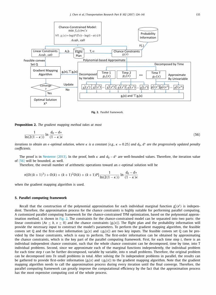
Fig. 2. Parallel framework.

Proposition 2. The gradient mapping method takes at most

1

ln (2(1 − κ)) ln

d 0 − d∗(1 − κ) ε

(56)

iterations to obtain an ε-optimal solution, where κ is a constant (e.g., κ = 0 . 25 ) and d 0 , d ∗ are the progressively updated penalty

coefficients.

The proof is in Nesterov (2013) . In the proof, both κ and d 0 − d ∗ are well-bounded values. Therefore, the iteration value

of (56) will be bounded, as well.

Therefore, the overall number of arithmetic operations toward an ε-optimal solution will be

n { O ((k + 1) 3 ) + O (k ) + (k + 1) 2 O (k ) + (k + 1) P } 1

ln (2(1 − κ)) ln

d 0 − d∗(1 − κ) ε

when the gradient mapping algorithm is used.

5. Parallel computing framework

Recall that the construction of the polynomial approximation for each individual marginal function g i t (x i ) is indepen-

dent. Therefore, the approximation process for the chance constraints is highly suitable for performing parallel computing.

A customized parallel computing framework for the chance-constrained TFM optimization, based on the polynomial approx-

imation method, is shown in Fig. 2 . The constraints for the chance-constrained model can be separated into two parts: the

linear constraints ( Ax ≤ b, x ≥ 0) and the chance constraints ( g t ( x )). The flight plan and the probability information will

provide the necessary input to construct the model’s parameters. To perform the gradient mapping algorithm, the feasible

convex set Q and the first-order information ( g t ( x ) and g t ( x )) are two key inputs. The feasible convex set Q can be pro-

vided by the linear constraints, which is easy to perform. The first-order information can be obtained by approximating

the chance constraints, which is the key part of the parallel computing framework. First, for each time step t , there is an

individual independent chance constraint, such that the whole chance constraint can be decomposed, time by time, into T

individual problems. Second, since we approximate each of the marginal functions independently, the individual problem

for each time step t can be further decomposed, variable by variable, into n small problems. Therefore, the original problem

can be decomposed into Tn small problems in total. After solving the Tn independent problems in parallel, the results can

be gathered to provide first-order information ( g t ( x ) and g t ( x )) to the gradient mapping algorithm. Note that the gradient

mapping algorithm needs to call the approximation process during every iteration until the final converge. Therefore, the

parallel computing framework can greatly improve the computational efficiency by the fact that the approximation process

has the most expensive computing cost of the whole process.


Fig. 3. Small-sized example.

Table 4

Flight schedule.

Flights f k ( t ) Origin Destination Route

f 1 [2,1,1,0,0,0,0,0,0,0,0] DTW CLE KDT W − ZOB 29 − ZOB 47 − ZOB 49 − KCLE

f 2 [2,1,1,0,0,0,0,0,0,0,0] CLE TOL K CLE − Z OB 49 − Z OB 47 − KT OL

f 3 [2,1,1,0,0,0,0,0,0,0,0] TOL ERI KT OL − ZOB 47 − ZOB 26 − ZOB 79 − KERI

f 4 [2,1,1,0,0,0,0,0,0,0,0] ERI DTW KERI − ZOB 79 − ZOB 26 − ZOB 29 − KDT W

f 5 [2,1,1,0,0,0,0,0,0,0,0] DTW TOL KDT W − ZOB 29 − ZOB 47 − KT OL

f 6 [2,1,1,0,0,0,0,0,0,0,0] CLE ERI K CLE − Z OB 49 − Z OB 79 − KERI

Table 5

Sector capacity distribution.

Capacity(C) 1 2 3 4

P ( C ) 0.0321 0.0871 0.2369 0.6439

6. Simulation results

6.1. Model validation with a small-sized example

6.1.1. Example setup

As stated in Section 3.1 , the brute-force MILP method has a limitation in handling large-scale real problems, but it

could provide accurate results for small-sized problems. Therefore, the MILP method could be an ideal contrast to the

approximation-based method if a small-sized TFM problem could be provided. In order to evaluate the accuracy of the novel

approximation-based method, a small-sized TFM problem is developed to perform the comparison. As shown in Fig. 3 , the

designed small TFM problem consists of five sectors (ZOB29, ZOB47, ZOB49, ZOB79, ZOB26 at the Cleveland Air Route Traffic

Control Center) and four airports (denoted as k 1 : DTW, k 2 : TOL, k 3 : CLE, k 4 : ERI ). The flight plan is shown in Table 4 , which

contains six flight routes with the corresponding departure schedule for each time step ( f k ( t )). Each flight is assumed to be

able to traverse each sector in one time period, and there are 11 planning time periods in total (note that these are abstract

periods and could be defined by real time periods, such as 15 min, in a full-scale problem). For simplification, the capacity

of each sector is assumed to be the same and set at a maximum of 4. All sectors are assumed to be independent and sub-

ject to the same probability distribution, given in Table 5 . The corresponding cumulative probability ( P ( C ≥ sn j )) is shown


Table 6

Cumulative probability : P ( C ≥ sn j ).

Number of flights( sn j ) 0 1 2 3 4 ≥ 5

P ( C ≥ sn j ) 1.0 1.0 0.9679 0.8808 0.6439 0

Table 7

Optimal flight flow based on MILP.

Time sn 1 sn 2 sn 3 sn 4 sn 5 P ≥ 0.8

0 0 0 0 0 0 1

1 0 0 0 0 0 1

2 3 2 2 0 0 0.825

3 1 3 1 2 2 0.825

4 2 2 1 0 3 0.825

5 1 3 2 1 2 0.825

6 2 2 2 2 2 0.849

7 1 3 2 1 2 0.825

8 1 1 1 2 0 0.9679

9 1 0 1 0 1 1

10 0 0 0 0 0 1

obj = 118

1 0 1 2 3 4 5 60

0.1

0.2

0.3

0.4

0.5

0.6

0.7

0.8

0.9

1

Pro

bab

ility

P(C

>=sn

j)

Number of flights assigned to the sector

Fig. 4. Cumulative probability.

in Table 6 , which represents the probability of satisfying the sector’s capacity limit when assigning sn j flights to that sector.

Note that if the sectors are not independent, then only the calculations of the joint probability distribution change, and the

method to form the feasible combination set of the MILP model is the same.

6.1.2. Result of MILP

The result of MILP is solved with the chance constraints’ significance level of 0.8 ( α = 0 . 8 ). The result is then collected

to check the feasibility of the chance constraint, which is shown in Table 7 . It is clear to see that the chance constraints

are all satisfied at each time step t . The original objective is 118, based on the MILP method, which is the accurate optimal

solution. Later, we will use this accurate optimal solution to evaluate the approximation-based method.

6.1.3. Result of approximation-based approach

To perform the approximation-based approach, a log-concave continuous probability distribution is provided, as shown

in Fig. 4 , which has the exact cumulative probability ( P ( C ≥ sn j )) with the discrete one in Table 5 . Therefore, the comparison

is meaningful with the same probability information. With the same significance level of 0.8 ( α = 0 . 8 ), the result, based on


Table 8

Optimal flight flow based on the approximation method in real value.


0 0 0 0 0 0 1

1 0 0 0 0 0 1

2 2.156 1.165 2.229 1.648 1.166 0.894

3 2.283 2.562 1.0 0 0 2.331 2.194 0.803

4 2.061 2.574 1.551 1.370 2.236 0.836

5 1.874 2.228 2.226 0.966 2.015 0.859

6 1.667 2.033 1.799 0.851 1.836 0.905

7 1.959 1.773 1.781 0.833 1.719 0.910

8 0.0 0 0 2.108 1.552 0.0 0 0 0.883 0.949

9 0.0 0 0 1.552 0.0 0 0 0.0 0 0 0.0 0 0 0.986

10 0.0 0 0 0.0 0 0 0.0 0 0 0.0 0 0 0.0 0 0 1

obj = 115.8

Table 9

Optimal flight flow based on the approximation method in

integer value.


0 0 0 0 0 0 1

1 0 0 0 0 0 1

2 2 1 3 0 1 0.853

3 2 3 0 2 2 0.800

4 3 2 2 0 2 0.800

5 2 3 2 1 2 0.800

6 0 2 2 2 2 0.878

7 2 2 2 0 0 0.907

8 0 2 1 1 0 0.968

9 0 1 0 2 1 0.968

10 1 0 0 0 2 0.968

obj = 121

the approximation-based method, is shown in Table 8 , which are real numbers before the rounding process. It is clear that

the approximation-based method could provide feasible optimal solutions, which also satisfy all of the chance constraints

for each time step t. The original objective is reduced to 115.8 because the feasible set of the integer problem is only a

subset of the real-valued problem. Thus, this smaller optimal objective is reasonable and could be evidence to demonstrate

that the approximation-based approach could achieve a valid real-valued optimal solution.

To achieve the integer-valued solution for the original problem, the Branch-and-Bound (B&B) algorithm is performed with

the Integer Programming solver Gurobi 6.02 ( Gurobi, 2014 ), where the real-valued optimal solution is provided as an initial

point. As shown in Table 9 , the rounding process provides a feasible integer-valued solution, which is sub-optimal, but very

close to the accurate optimal integer solution. There are two reasons for the sub-optimal solution: first, there are errors

in the approximation process, since we only choose the polynomial with a finite degree to approximate the original chance

constraints; second, only a simple B&B cutting process is performed to achieve the integer result. Although it is sub-optimal,

the error between the two objectives is only 3%. Thus, it is reasonable to believe that the approximation-based approach

could provide a reliable integer solution to the chance-constrained TFM problem, which is also confirmed by large-scale

problem simulations in Section 6.2 .

6.2. Large-scale ATFM simulation

This subsection presents a large-scale ATFM optimization, employing the proposed parallel computing framework. The

traffic data are extracted from the ASDI, which provides historical traffic data, as well as flight plans. A 2-h NAS-wide in-

stance is used, which represents the high-traffic period of a day, with 2326 paths and 3054 flights involved. The same

log-concave probability distribution in Section 6.1 is adopted and adjusted, according to the real-sector capacity (usually

10 to 15). The optimization is performed on a small Spark cluster with six nodes, where Spark is a distributed computing

platform ( Karau et al., 2015 ). Each node of the Spark cluster is a DELL workstation configured with an 8-processor CPU. All

workstations run UBUNTU 14.04 with Spark 1.3.1. The optimization subproblems were solved by calling Gurobi 6.0.2.

To further demonstrate that the approximation-based approach could provide a reliable solution, several large-scale ATFM

cases with different problem sizes are tested. Since the size of the ATFM problem is highly related to the number of sectors,

the simulation plans with various number of sectors are extracted from the 2-h NAS-wide instance above. Fig. 5 shows the

relative objective error between the approximation-based approach and the accurate optimal solution. The error gap is kept

below 5% with various number of sectors from 5 to 20, which confirmed that the quality of approximation-based solution is

also reliable for large-scale ATFM problems. Due to the exponentially growing complexity of the MILP method, we only test


5 10 15 200

0.5

1

1.5

2

2.5

3

3.5

4

4.5

5

rela

tive

err

or

%

number of sectors

Fig. 5. Relative error with different ATFM problem sizes.

up to 20 sectors. Actually, the approximation-based approach can handle large-scale problem with more than 20 sectors,

but it is difficult to get the accurate optimal solution for comparison.

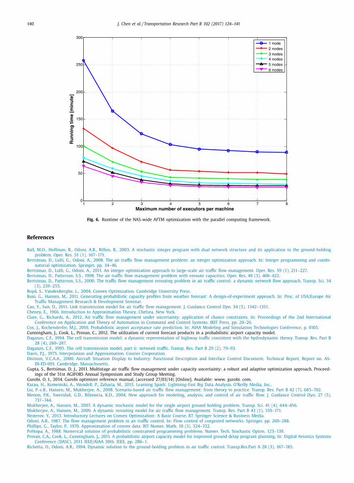
The running time of the optimization with different paralleling configurations is demonstrated in Fig. 6 . As a tuning

parameter to control the concurrency level, the maximum number of executors allowed on a node can be adjusted. Since the

8-processor CPU can handle 8 threads simultaneously, the maximum number of executors per machine can be up to eight.

The running time decreases when more executors are used for a fixed number of nodes. However, the speedup is not linear

and becomes less noticeable as the number of executors approaches 8. The reason is the increasing overhead for allocating

CPU time to the processors. Another speedup pattern can be observed as more nodes are launched. The speedup is also not

linear by the fact that it is more and more difficult to achieve further speedup as more nodes are deployed. The runtime is

reduced from 241 min with 1 nodes and 1 executor to 25 min with 6 nodes and 8 executors. The speedup increases about

tenfold, which is less than the theoretical 6 × 8 = 48 times. This is due to the increasing overhead for the synchronization

and communication between nodes, which is a common issue in parallel computing programming. Overall, it is clear that

the parallel computing framework, indeed, improves the computational efficiency of the polynomial approximation-based

approach.

7. Conclusions

This paper introduces a novel polynomial approximation-based chance-constrained optimization method to address un-

certainty in ATFM, which could provide a computationally efficient algorithm. Based on a previous deterministic Integer

Programming optimization model of ATFM, a chance-constrained model is developed to include probabilistic sector capac-

ity constraints. Then, a polynomial approximation-based approach is applied to efficiently solve such a large-scale chance-

constrained optimization problem. The approximation is based on the numerical properties of the Bernstein polynomial,

which is capable of effectively controlling the approximation error for both the function value and gradient. Thus, the

gradient mapping (a first-order algorithm) is adopted to obtain a satisfactory solution which is expected to be optimal.

Numerical results are reported to evaluate the polynomial approximation-based approach by comparing it with the brute-

force method, which demonstrates that the approximation-based approach could provide reliable solutions. Moreover, a dis-

tributed computing framework is designed based on the massive independent approximation processes in the polynomial

approximation-based approach, which is demonstrated with the ability to improve computational efficiency. This chance-

constrained optimization method and its computation platform are potentially helpful in their application to many domains

in air transportation. This method and platform are not only limited to ATFM, but can also be extended to airport surface

operations and airline management under uncertainties.


1 2 3 4 5 6 7 80

50

100

150

200

250

300

Ru

nn

ing

tim

e [m

inu

te]

Maximum number of executors per machine

1 node2 nodes3 nodes4 nodes5 nodes6 nodes

Fig. 6. Runtime of the NAS-wide AFTM optimization with the parallel computing framework.

References

Ball, M.O. , Hoffman, R. , Odoni, A.R. , Rifkin, R. , 2003. A stochastic integer program with dual network structure and its application to the ground-holdingproblem. Oper. Res. 51 (1), 167–171 .

Bertsimas, D. , Lulli, G. , Odoni, A. , 2008. The air traffic flow management problem: an integer optimization approach. In: Integer programming and combi-natorial optimization. Springer, pp. 34–46 .

Bertsimas, D. , Lulli, G. , Odoni, A. , 2011. An integer optimization approach to large-scale air traffic flow management. Oper. Res. 59 (1), 211–227 .

Bertsimas, D. , Patterson, S.S. , 1998. The air traffic flow management problem with enroute capacities. Oper. Res. 46 (3), 406–422 . Bertsimas, D. , Patterson, S.S. , 20 0 0. The traffic flow management rerouting problem in air traffic control: a dynamic network flow approach. Transp. Sci. 34

(3), 239–255 . Boyd, S. , Vandenberghe, L. , 2004. Convex Optimization. Cambridge University Press .

Buxi, G. , Hansen, M. , 2011. Generating probabilistic capacity profiles from weather forecast: A design-of-experiment approach. In: Proc. of USA/Europe AirTraffic Management Research & Development Seminar .

Cao, Y. , Sun, D. , 2011. Link transmission model for air traffic flow management. J. Guidance Control Dyn. 34 (5), 1342–1351 .

Cheney, E. , 1966. Introduction to Approximation Theory . Chelsea, New York. Clare, G. , Richards, A. , 2012. Air traffic flow management under uncertainty: application of chance constraints. In: Proceedings of the 2nd International

Conference on Application and Theory of Automation in Command and Control Systems. IRIT Press, pp. 20–26 . Cox, J. , Kochenderfer, M.J. , 2016. Probabilistic airport acceptance rate prediction. In: AIAA Modeling and Simulation Technologies Conference, p. 0165 .

Cunningham, J., Cook, L., Provan, C., 2012. The utilization of current forecast products in a probabilistic airport capacity model. Daganzo, C.F. , 1994. The cell transmission model: a dynamic representation of highway traffic consistent with the hydrodynamic theory. Transp. Res. Part B

28 (4), 269–287 .

Daganzo, C.F. , 1995. The cell transmission model, part ii: network traffic. Transp. Res. Part B 29 (2), 79–93 . Davis, P.J. , 1975. Interpolation and Approximation. Courier Corporation .

Division, V.C.A .A . , 20 0 0. Aircraft Situation Display to Industry: Functional Description and Interface Control Document. Technical Report, Report no. AS-DI-FD-001. Cambridge, Massachusetts .

Gupta, S., Bertsimas, D. J., 2011. Multistage air traffic flow management under capacity uncertainty: a robust and adaptive optimization approach. Proceed-ings of the 51st AGIFORS Annual Symposium and Study Group Meeting.

Gurobi, O. I., 2014. Gurobi optimizer reference manual, (accessed 27/03/14) [Online]. Available: www. gurobi. com.

Karau, H. , Konwinski, A. , Wendell, P. , Zaharia, M. , 2015. Learning Spark: Lightning-Fast Big Data Analysis. O’Reilly Media, Inc. . Liu, P.-c.B. , Hansen, M. , Mukherjee, A. , 2008. Scenario-based air traffic flow management: from theory to practice. Transp. Res. Part B 42 (7), 685–702 .

Menon, P.K. , Sweriduk, G.D. , Bilimoria, K.D. , 2004. New approach for modeling, analysis, and control of air traffic flow. J. Guidance Control Dyn. 27 (5),737–744 .

Mukherjee, A. , Hansen, M. , 2007. A dynamic stochastic model for the single airport ground holding problem. Transp. Sci. 41 (4), 4 4 4–456 . Mukherjee, A. , Hansen, M. , 2009. A dynamic rerouting model for air traffic flow management. Transp. Res. Part B 43 (1), 159–171 .

Nesterov, Y. , 2013. Introductory Lectures on Convex Optimization: A Basic Course, 87. Springer Science & Business Media .

Odoni, A.R. , 1987. The flow management problem in air traffic control. In: Flow control of congested networks. Springer, pp. 269–288 . Phillips, G. , Taylor, P. , 1970. Approximation of convex data. BIT Numer. Math. 10 (3), 324–332 .

Prékopa, A. , 1988. Numerical solution of probabilistic constrained programming problems. Numer. Tech. Stochastic Optim. 123–139 . Provan, C.A. , Cook, L. , Cunningham, J. , 2011. A probabilistic airport capacity model for improved ground delay program planning. In: Digital Avionics Systems

Conference (DASC), 2011 IEEE/AIAA 30th. IEEE, pp. 2B6–1 . Richetta, O. , Odoni, A.R. , 1994. Dynamic solution to the ground-holding problem in air traffic control. Transp.Res.Part A 28 (3), 167–185 .

http://refhub.elsevier.com/S0191-2615(16)30606-3/sbref0001

















































































Saumard, A. , Wellner, J.A. , 2014. Log-concavity and strong log-concavity: a review. Stat. Surv. 8, 45 . Shapiro, A. , Dentcheva, D. , et al. , 2014. Lectures on Stochastic Programming: Modeling and Theory, 16. SIAM .

Sridhar, B. , Grabbe, S.R. , Mukherjee, A. , 2008. Modeling and optimization in traffic flow management. Proc. IEEE 96 (12), 2060–2080 . Stewart, G. , 1993. Afternotes on Numerical Analysis. University of Maryland at College Park .

Sun, D. , Bayen, A.M. , 2008. Multicommodity eulerian-lagrangian large-capacity cell transmission model for en route traffic. J. Guidance Control Dyn. 31 (3),616–628 .

Sun, D. , Clinet, A. , Bayen, A.M. , 2011. A dual decomposition method for sector capacity constrained traffic flow optimization. Transp. Res. Part B 45 (6),

880–902 . Sun, D. , Sridhar, B. , Grabbe, S.R. , 2010. Disaggregation method for an aggregate traffic flow management model. J. Guidance Control Dyn. 33 (3), 666–676 .

Van der Vaart, A.W. , 20 0 0. Asymptotic Statistics, 3. Cambridge University Press . Volpe, N.T.C. , 20 0 0. Enhanced Traffic Management System (ETMS). Technical Report, Rep. VNTSC-DTS56-TMS-002. United States Department of Transporta-

tion, Cambridge, Massachusetts . Wei, P. , Cao, Y. , Sun, D. , 2013. Total unimodularity and decomposition method for large-scale air traffic cell transmission model. Transp. Res. Part B 53, 1–16 .

































transportation research part b - purdue university

Documents