transport properties of polystyrene above and a …

TRANSPORT PROPERTIES OF POLYSTYRENE ABOVE AND

BELOW THE GLASS TRANSITION TEMPERATURE

by

LAWRENCE ROBERT FIKE, B.S. in Chem.

A THESIS

IN

CHEMICAL ENGINEERING

Submitted to the Graduate Faculty of Texas Tech University in

Partial Fulfillment of the Requirements for

the Degree of

MASTER OF SCIENCE

CHEMICAL ENGINEERING

Approved

Accepted

December, 1983

n

7-f.

L- " ^

• ' ' \ /

r"

1*

„ "» '

ACKNOWLEDGMENTS

The author expresses his extreme gratitude and thanks to the

following people:

Dr. R. W. Tock, chairman of the committee, for his technical advice

and endless enthusiasm throughout the completion of this study.

Dr. Fred Senatore, committee member, for his helpful suggestions

and support.

Most of all, my wife, Shannon, for her patience, understanding and

encouragement during the course of this work.

Also, the financial support of Cosden Oil and Chemical Company is

gratefully acknowledged.

n

TABLE OF CONTENTS

ACKNOWLEDGMENTS

ABSTRACT

LIST OF FIGURES

CHAPTER I INTRODUCTION

CHAPTER II LITERATURE REVIEW

Viscosity Above Glass Transition and Below Melt Temperature ,

Mass Transfer Diffusion Coefficients

CHAPTER III EXPERIMENTAL APPARATUS ,

Viscosity Measurement

Mass Diffusion Coefficient Measurement

CHAPTER IV EXPERIMENTAL PROCEDURE ,


Mass Diffusion Coefficient Measurement....,

CHAPTER V THEORY

Theoretical Approach to the Measurement of Viscosity

Theoretical Approach to the Measurement of Shear Modulus

Theoretical Approach to the Measurement of Mass Diffusion Coefficient

CHAPTER VI RESULTS OF VISCOSITY MEASUREMENTS

Above the Melt Temperature ,

Below the Glass Transition Temperature

Below the Melt Temperature and Above the Glass Transition Temperature ,

iii

PAGE

ii

v

vi

1

3

3

9

17

17

20

22

22

22

25

25

28

30

46

48

48

50

CHAPTER VII RESULTS OF SHEAR MODULUS MEASUREMENTS...

CHAPTER VIII RESULTS OBTAINED FOR MASS DIFFUSION

COEFFICIENTS

CHAPTER IX CONCLUSION

REFERENCES

APPENDIX A EXPERIMENTAL DATA FOR VISCOSITY AND SHEAR MODULUS

APPENDIX B EXPERIMENTAL DATA FOR MASS DIFFUSION COEFFICIENT OF WATER THROUGH POLYSTYRENE

APPENDIX C EXPERIMENTAL DATA FOR MASS DIFFUSION COEFFICIENT OF N-PENTANE THROUGH POLYSTYRENE ,

APPENDIX D COMPUTER PROGRAM FOR MATHEMATICAL MODEL TO PREDICT BEAD DENSITY OF POLYSTYRENE DURING THE EXPANSION PROCESS

PAGE

53

55

61

62

63

68

70

73

TV

ABSTRACT

In the production of expandable polystyrene (EPS) foam, it is

desirable to be able to predict the density of the final product by some

means other than empirical estimates. Therefore, a mathematical model

was developed to predict the density of EPS during a prepuffing

expansion process. Use of the mathematical model requires some knowledge

of the fundamental properties of viscosity, shear modulus, and mass

diffusion coefficients for water and n-pentane through polystyrene.

Since expansion is induced by thermal stimulus, these properties must be

known as a function of temperature. The theoretical and experimental

development in measuring these parameters constitute the bulk of the

text in this thesis. A very simplistic Maxwell model for viscoelastic

behavior was used as the basis for the theoretical development in the

determination of the viscosity and shear modulus of polystyrene. Mass

diffusion coefficients for water and n-pentane in polystyrene were

determined by a solution to Fick's second law with appropriate initial

and boundary conditions. Once the parameters had been determined, they

were fit to an Arrhenius type model in order to determine temperature

dependence. The transport properties were observed to be strongly

affected by the polymer's glass transition. Finally, a computer program

was developed and used to predict the density of EPS as a function of

time during the expansion process.

LIST OF FIGURES

PAGE

Figure 1. Schematic representation of the Maxwell Model 4

Figure 2. Curve of stress vs. time 10

Figure 3. Stress-strain rate curve of a power law fluid 11

Figure 4. Graphical solution to Fick's second law for spherical solids 13

Figure 5. Mass diffusion coefficients for n-pentane through polystyrene above and below the glass transition temperature 14

Figure 6. Schematic representation of apparatus to

measure the viscosity of polystyrene 18

Figure 7. Instron Model 1122 (Instron sales literature) 19

Figure 8. Schematic representation of apparatus to measure mass diffusion coefficient for water through polystyrene 21

Figure 9. ASTM standard polymer bar 23

Figure 10. Schematic representation of a generated readout from the recording apparatus of the Instron 26

Figure 11. Schematic representation of a typical stress-strain plot 30

Figure 12. Weight loss vs. time for the isotherm T = 50 deg C 33





VI

PAGE




Figure 20. Weight loss of water vs. time for the i sotherm T = 50 deg C 42


Figure 22. Weight loss of water vs. time for the isotherm T = 100 deg C 44


Figure 24. Plot of the natural logarithm of the calculated viscosity at several different strain rates vs. reciprocal of absolute temperature 47

Figure 25. Schematic representation of a stress-strain rate piot 49

Figure 26. Natural logarithm of apparent viscosity vs. the reciprocal of absolute temperature 51

Figure 27. Natural logarithm of apparent viscosity vs. the reciprocal of absolute temperature 52

Figure 28. Natural logarithm of the shear modulus vs. the reciprocal of absolute temperature 54

Figure 29. Natural logarithm of the mass diffusion coefficient for water through polystyrene vs. the reciprocal of absolute temperature 56

Figure 30. Natural logarithm of the mass diffusion coefficient for n-pentane through polystyrene vs. the reciprocal of absolute temperature 58

vn

CHAPTER I

INTRODUCTION

In the manufacture of expandable polystyrene foam (EPS), it is of

great importance to be able to predict the density of the final product.

EPS is marketed according to grades. The bead size and density determine

the grade of the product. The bead size can be determined by screening

operations. The bead density, however, can be somewhat variable. In most

instances, the density must be predicted by empirical methods. A more

theoretically based approach is desirable and as will be shown in this

dissertation, perhaps possible.

Polystyrene is the product of a reaction of styrene monomer by

suspension polymerization in which spherical beads are formed. The

polymer is made "expandable" by impregnating the beads with n-pentane

which becomes the blowing agent. The impregnated bead can be expanded by

a process known as prepuffing. The prepuffing operation involves the

contact of 220 deg F steam with the beads in a fluidized bed type

arrangement. The heat causes the n-pentane to reach a superheated state.

The high vapor pressure which builds up causes void spaces to develop

and the bead, which is in a softened state, expands. It has been

suggested that during the prepuffing operation, viscosity and mass

diffusion coefficients through polystyrene control the expansion of the

beads. Surprisingly, it can also be shown that heat transfer is

unimportant as a rate controlling step during the expansion process.

This is due to the fact that the thermal diffusivity of the beads is

many orders of magnitude greater than the mass diffusivity. Hence,

thermal gradients disappear rather rapidly in comparison to concentra

tion and momentum gradients.

Research at Texas Tech has resulted in the development of a

mathematical model describing the expansion process, which has improved

the ability to predict the density of EPS during the prepuffing stage.

The model was developed by performing a force balance on the stretching

surfaces of a hypothetical bead of polystyrene. The result of this model

is a series of equations which must be solved simultaneously. From these

equations, a theoretical EPS bead density can be determined at any time

during the prepuffing operation.

The objective of this study was to collect all the material

property information needed to solve the above mentioned equations. This

included the measurement of melt viscosity and shear modulus of

polystyrene over a wide temperature range (70 deg F - 200 deg F).

Moreover, the mass diffusion coefficients for n-pentane and water

through polystyrene had to be determined for this same temperature

range.

CHAPTER II

LITERATURE REVIEW

The viscosity and mass diffusion coefficients of simple, pure

substances can usually be obtained with great accuracy provided the

proper instrumentation is available. However, even the most sophis

ticated instruments are inadequate in many industrially important

systems and simplifications must be made in order to determine just the

order of magnitudes of these transport properties. The theories used in

collecting the data needed for these properties are those suitably

compatible with the information which can be obtained from available

instrumentation. The methods of this study are simplified but give

reasonable and reliable measurements of viscosity and mass diffusion

coefficients.

Viscosity Above Glass Transition and Below Melt Temperature

The methodology for determining the temperature dependence of the

viscosity for polystyrene was as follows. Polystyrene was assumed to be

viscoelastic below its melt temperature. A viscoelastic material

exhibits solid-like elastic properties along with fluid-like viscous

properties. A Maxwell model, illustrated schematically in Figure 1, has

been used as a simplified mechanical representation of a viscoelastic

material (Richard W. Hanks, 1970). Other more sophisticated models exist

in the literature but the simplicity of the Maxwell model gives results

suitable for this study. As shown, the model consists of a Hookean

spring connected in series with a Newtonian fluid dashpot. The Hookean

F/A

i

c

Hookean Spring

\ \ \ V V \ '

Newtonian Dashpot

Figure 1. Schematic representation of the Maxwell model

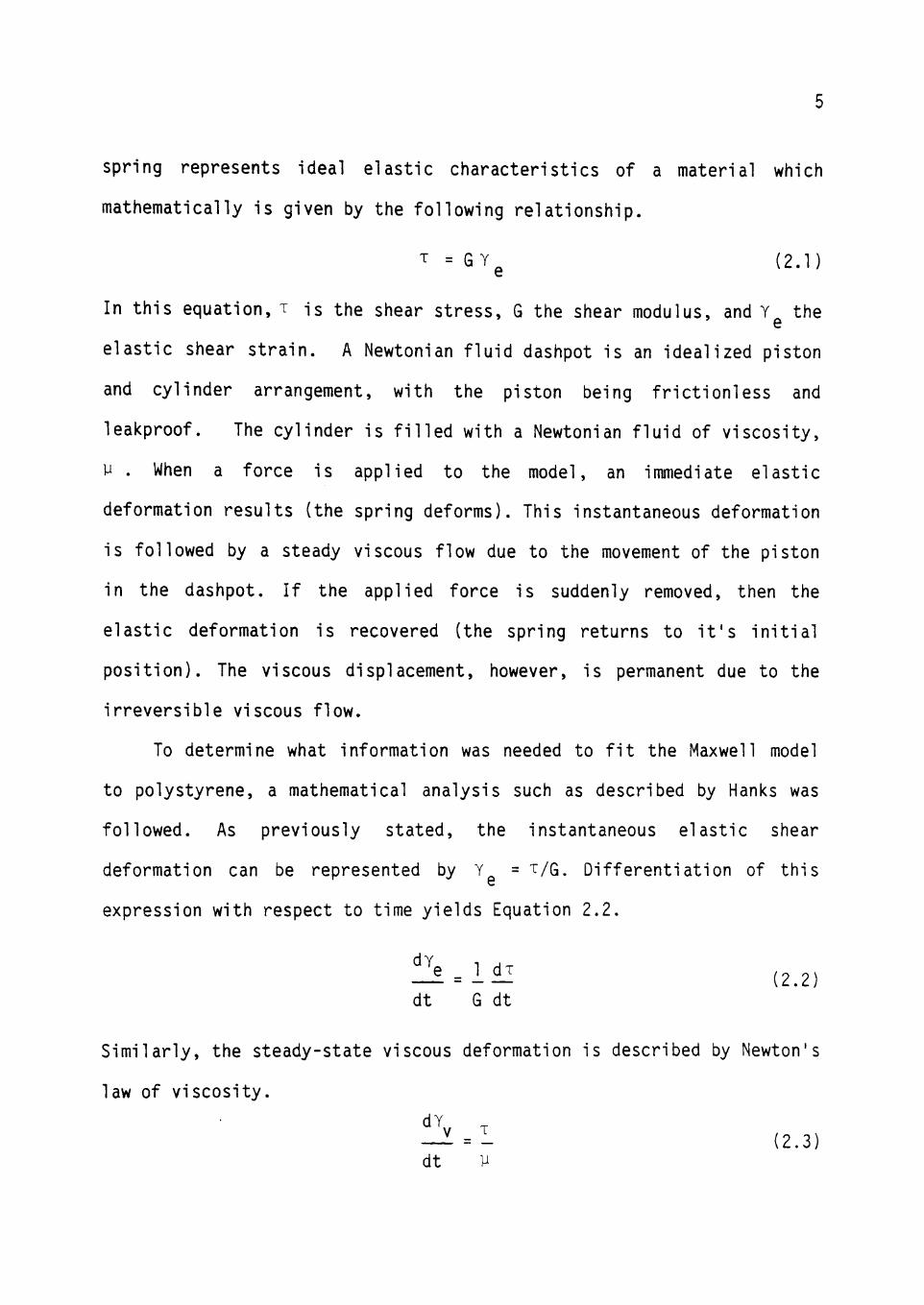
spring represents ideal e last ic characterist ics of a material which

mathematically is given by the fol lowing relat ionship.

^ = GYg (2.1)

In this equation, T is the shear stress, G the shear modulus, and Y the

elastic shear strain. A Newtonian fluid dashpot is an idealized piston

and cylinder arrangement, with the piston being frictionless and

leakproof. The cylinder is filled with a Newtonian fluid of viscosity,

y . When a force is applied to the model, an immediate elastic

deformation results (the spring deforms). This instantaneous deformation

is followed by a steady viscous flow due to the movement of the piston

in the dashpot. If the applied force is suddenly removed, then the

elastic deformation is recovered (the spring returns to it's initial

position). The viscous displacement, however, is permanent due to the

irreversible viscous flow.

To determine what information was needed to fit the Maxwell model

to polystyrene, a mathematical analysis such as described by Hanks was

followed. As previously stated, the instantaneous elastic shear

deformation can be represented by Y = ^/G. Differentiation of this

expression with respect to time yields Equation 2.2.

' ' ' - ' '^ (2.2) dt G dt

Simi lar ly , the steady-state viscous deformation is described by Newton's

law of v iscosi ty .

dt y

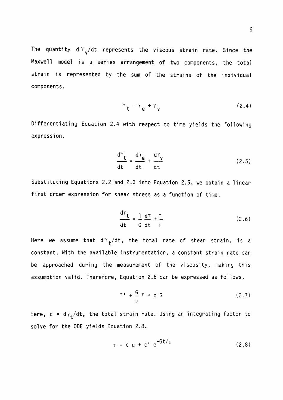
The quantity d Y^/dt represents the viscous strain rate. Since the

Maxwell model is a series arrangement of two components, the total

strain is represented by the sum of the strains of the individual

components.

Differentiating Equation 2.4 with respect to time yields the following

expression.

dY dY dY

-± = -± + -1 (2.5) dt dt dt

Substituting Equations 2.2 and 2.3 into Equation 2.5, we obtain a linear

first order expression for shear stress as a function of time.

^ = 1 ^ . 1 (2.6) dt G dt y

Here we assume that dY./dt, the total rate of shear strain, is a

constant. With the available instrumentation, a constant strain rate can

be approached during the measurement of the viscosity, making this

assumption valid. Therefore, Equation 2.6 can be expressed as follows.

T' + i T = c G (2.7) y

Here, c = dY.,-/dt, the total strain rate. Using an integrating factor to

solve for the ODE yields Equation 2.8.

T = c y + c' e"^^^^ (2.8)

The constant of integration is c' and t is time. According to the

Maxwell model, at t = 0, the shear stress must also be equal to zero.

Using this as an initial condition, the constant of integration can be

expressed.

c' = - c y

Substitution into Equation 2.8 gives a working equation.

T = c y ( l - e"^^^^) (2.9)

Inspection of Equation 2.9 suggests that when t is sufficiently large,

the quantity e will approach zero and thereafter pure viscous

deformation results.

T = cy (2.10) t^^

Here, c is s t i l l the tota l strain rate, which is constant, and Ts is the It--'

shear stress as the time becomes large. Equation 2.10 is rearranged to

give the following form.

\^ = /c (2.11)

Although the shear stress, ^ , could not be measured d i rect ly with

the available instrumentation, an alternative solution was found. This

is based on the relat ionship between elast ic moduli; the shear modulus

G, Young's modulus E, and Poisson's ra t io ^ for an isotropic material

(Richard W. Hanks, 1970). The relat ionship is as fol lows.

E = 2G(1 + v ) (2.12)

8

The shear modulus was defined earlier as Equation 2.13.

G = T/Yg (2.13)

The Young's modulus can be defined as the ratio of the tensile stress to

the tensile strain.

E =1 (2.14)

Substituting Equations 2.13 and 2.14 into Equation 2.12 and noting that

Y = £ for small strain leads to the following expression.

a = 2T(1 + v) (2.15)

Poisson's ratio is defined as the negative ratio of the strain in the

transverse direction of an applied stress to the strain in the direction

of stress. By assuming the polymer is in the rubbery region (purely

elastic), we can approximate Poisson's ratio by assuming it to be 0.5.

Substitution eliminates v from Equation 2.15.

T = l a (2.16) 3

The tensile strength cr is a quantity that can be measured with the

Instron. Therefore, substituting Equation 2.16 into 2.11 yields Equation

2.17.

y =a/3c .2.17)

A value for the viscosity y can now be obtained experimentally from a

measurement of tensile strength at a known constant strain rate after

sufficient time has elapsed. From Figure 2, the measured value for the

tensile stress is shown as ^., This can be used with Equation 2.17 and a

constant strain rate to calculate the value for the viscosity of

polystyrene below its melt temperature. Since Poisson's ratio changes

below the glass transition temperature, the same calculation is an

approximation of viscosity below the glass transition temperature.

Viscosities above the melt temperature were obtained using a

capillary rheometer and the Instron. Polystyrene above its melt

temperature has a more purely viscous behavior. Its stress-strain rate

curve, shown in Figure 3, follows the power law. A power law fluid is

characterized by an expression as follows.

T= K Q ( Y ) "

Here, K is a temperature dependent parameter called the consistency

factor, Y the strain rate, and n is a constant ranging between 0 and 1

(for viscoelastic materials). The viscosity is obtained by finding the

shear stress at a strain rate of one on a stress-strain curve and

substituting it into the equation y = T/Y. The capillary rheometer is an

isothermal apparatus and when used in conjunction with the Instron,

gives a value for the tensile strength at a given constant strain rate.

Mass Transfer Diffusion Coefficients

The acquisition of a diffusion coefficient for n-pentane through

polystyrene is based on Fick's second law.

S 2 — i : = D v^ C. 9t

10

E

Stress

Figure 2. Curve of stress vs. time.

11

CO CO

<u +J CO

strain Rate

Figure 3. Stress-strain rate curve of a power law fluid,

12

Here C^ is the concentration of n-pentane in the bead, D the diffusion

coefficient, and t is time. Graphical solutions of Fick's second law for

certain initial and boundary conditions can be found in most mass

transfer texts. The shape of the curve depends on the geometry of the

solid. It was assumed that a polystyrene bead is a perfect sphere with

radius, R. A typical graphical solution is shown in Figure 4 (Robert E.

Treybal, 1980). Boundary and initial conditions for this particular

solution require that concentrations at the surface of the bead be

constant, and that the bead initially must have a uniform internal

concentration. The curve represents a proportionality between the

fraction of pentane unremoved from the polystyrene bead, (C« , ) - (C, 00

2 /Cy 0 ' ^A °°^' " ^^^ quantity Dt/R . C« , is the average concentration

inside the bead at some time t and C. , the concentration at the

surface of the bead.

Using this graphical approach, mass diffusion coefficients well

above and below the glass transition temperature were obtained. These

were compared with data obtained from the literature. Data found in the

literature is shown in Figure 5.

A different approach was used to determine the mass diffusion

coefficient of water through polystyrene. A fluid diffusing through a

solid film has a characteristic lag time to reach steady state. This lag

time is that time required for the fluid, which is first introduced to

one side of a solid film, to migrate through the film and emerge from

the other side. Estimations of water vapor diffusion coefficients in

polystyrene are based on the assumptions that the diffusion coefficient

is independent of concentration, and that the film is initially

13

o

«a:

CJ

Dt/R'

Figure 4. Graphical solution to Fick's second law for spherical solids.

14

16-j

•17

-18-

-19-

•20-

-2J -

(/J

CVJ E u

I I

c

-22-

-23-

•2H-

-25-

-26-

-27- I I I I I I I I I I I I I i - i - r ' i - i ' i !• I I I I I I I !• > I I I I r ' I I I I I I ' l I I I I I I I I I ' l I I I I I

0.0020 0.0022 0.002H 0.0026 0.0028 0.0030 0.0Q32

1A(K)

Figure 5. Mass diffusion coefficients for n-pentane through polystyrene above and below the glass transition temperature.

15

completely free of water. Also, water was continually removed from the

low concentration side of the polymer film. The amount of water which

passes through the film at any time is described as follows (Crank,

1968).

' = 5 t . i . 2 _ ^ Ml! ! exp(ienilit) ( .19) ^ ^ 1 5 2 6 ^ 2 2

T ^ ^ n= l "

Here, Q is the amount of water vapor which has passed through the film,

^ is the film thickness, and C-, is the concentration of water on the

high concentration side of the film. As time becomes large, some

steady-state will be approached and the exponential term will become

negligibly small. Therefore, Equation 2.19 reduces to the following

relationship.

Q = — L (t - — ) (2.20) ^ 6D

A plot of Q versus time eventually leads to a linear plot. The

extrapolated intercept of this plot (i.e., Q = 0) is denoted as the lag

time.

t, = — (2.21) ^^9 60

The diffusion coefficient can then be approximated directly from the

following equation.

^2 D = (2.22)

lag

16

Here ^ is the film thickness and t, „ is the lag time. The constant on 1 ag

the right-hand side of Equation 2.22 is dependent upon the geometry of

the solid. Good results are obtained with use of this equation. Very

little data for water through polystyrene were found in the literature.

CHAPTER III

EXPERIMENTAL APPARATUS


Much of the viscosity of polystyrene was obtained using an Instron

Model 1122 and the Maxwell model previously described. However, in

order to determine the temperature influence on the viscosity, an appar

atus to maintain a constant temperature was constructed. A rectangular

box was built to enclose the grips of the Instron. These grips transfer

forces to the polystyrene during the measurement. Hinges were added to

the front side of the box to provide access. Fiberglass insulation was

added to the inside of the box to help retain heat which was supplied

from a 1500 watt hair dryer. The nozzle of the hair dryer was inserted

through a 3 inch diameter hole near the bottom of the back side of the

box. The nozzle was angled upward toward one side of the box to help

increase circulation of air. To assure that a constant temperature was

maintained within the box, a Thermo Electric temperature controller was

connected through a switch to the hairdryer. Two holes were also drilled

into the front face of the box and thermometers were inserted. This

permitted the temperatures down the length of the polymer sample to be

monitored. The apparatus yielded a constant temperature within the box

of + 5 deg F over a temperature range of 70 deg F to 220 deg F. The

apparatus is depicted schematically in Figure 6. The Instron is shown in

Figure 7.

17

18

Thermo E Temperature Controller

Figure 6. Schematic representation of apparatus to measure the viscosity of polystyrene.

I I I 1 I I • H i ! 11,1-

19

Figure 7. Instron Model 1122 (Instron sales literature)

20


The mass diffusion coefficients of water and n-pentane through

polystyrene were obtained using two different techniques. For water, an

evaporation cup was used. With this apparatus, water is placed in an

aluminum cup. Polystyrene film is then placed over the top of the cup.

An 0-ring is placed between the metal of the cup and the polystyrene

film to assure that all the water transferred from the cup is by

diffusion. A wire screen is put on top of the polystyrene film to pro

vide support as internal pressure builds. An annular aluminum clamp is

then added to the top of the film and screen, leaving the top surface of

the polystyrene exposed to the atmosphere. The apparatus is clamped

tightly with three C-clamps. This apparatus is shown schematically in

Figure 8. To create a pressure drop across the polystyrene film and to

determine the mass diffusion coefficient at several different tempera

tures, the cup was placed in a Precision Scientific Model 524 vacuum

oven, which could be held at a constant temperature.

Another technique was required to determine a mass diffusion coef

ficient for n-pentane. This was necessary because with the evaporation

cup, the n-pentane tended to dissolve the polystyrene film which result

ed in a loss of n-pentane by means other than diffusion. Therefore,

polystyrene beads containing approximately 6 weight percent n-pentane

were used. A specified mass of these beads were placed in a beaker which

was then inserted into a vacuum oven. The diffusion of n-pentane out of

the beads was then recorded as a weight loss for the bead mass.

21

Annular Clamp

Wire Screen

Polystyrene Film

0-Ring

Aluminum Cap

Figure 8. Schematic representation of apparatus to measure mass diffusion coefficient for water through polystyrene.

CHAPTER IV

EXPERIMENTAL PROCEDURE


Viscosities of polystyrene were measured at temperature isotherms

of 79, 100, 130, 160, and 190 deg F. An ASTM standard 8 and 1/2 inch

polymer bar (see Figure 9) was inserted into the grips of the Instron.

The grips were separated by a distance of 4 inches. After the tempera

ture controller was adjusted to the desired setting, heat was introduced

inside the box until an equilibrium steady-state temperature was obtain

ed. The two thermometers were checked regularly to assure a constant

temperature. For each temperature, the crosshead speed of the Instron

was varied from 0.005 to 1 inch per minute. Tensile force versus time

was automatically recorded on chart paper. From this information, the

viscosities could be calculated for each isotherm.


Use of the evaporation cup to determine mass diffusion coefficients

for water through polystyrene is as follows. The cup was filled with

distilled water and the 0-ring, polymer film, and wire screen were plac

ed on top. The cup assembly containing water was then weighed to four

decimal places on a Mettler balance. The cup was then fastened and

tightened using the three C-clamps. This apparatus was inserted in the

vacuum oven at a selected temperature. For each run a vacuum of 18

inches of mercury was maintained. Runs anywhere from 6 hours to 3 days

22

23

0.75"

h

S L T

4"

0.5"

/

2.25"

Figure 9. ASTM standard polymer bar.

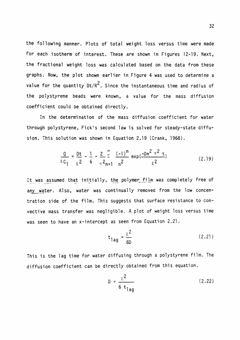
24

in duration were made. After each run, the evaporation cup was undamp

ed, allowed to cool to room temperature, and reweighed on the Mettler

balance. The weight loss of water versus time was recorded.

Mass diffusion coefficients for n-pentane were obtained in the

following manner. A mass of beads weighing 4-6 grams and containing

approximately 6 weight percent n-pentane were placed in a beaker. This

beaker was placed in an oven at a selected test temperature. In order to

prevent the beads from expanding too quickly, a vacuum was not applied

to the oven. The beaker was left in the oven for approximately 15

minutes. After this period of time, the beaker was placed in a desic

cator where it was allowed to cool to room temperature. The beads were

then reweighed on the Mettler balance and the weight loss versus time

was recorded. The beads were placed back into the oven and this proce

dure was continued until no further weight loss could be detected.

CHAPTER V

THEORY

Theoretical Approach to the Measurement of Viscosity

The readout of the recording apparatus of the Instron is an analog

of the stress versus strain curve for the material being tested. A sche

matic representation of a typical curve generated by the Instron is

shown in Figure 10. The viscosity of the test specimen was determined

directly from the information obtained from this type of graph. As shown

earlier, the apparent viscosity of polystyrene is approximated using the

Maxwell model. This model represents the total strain of a viscoelastic

material to be the sum of the strains for the total elastic and total

viscous portions of the model and was described previously in Equation

2.4.

Y^ = Y + Y (2.4) t e V

Taking the derivative of this equation with respect to time yields the

expression shown in Equation 2.5

dY. dY^ dY, _ 1 = — i + - l (2.5) dt dt dt

Equations 2.2 and 2.3 were shown earlier and substituted in Equation 2.5

to yield Equation 2.6.

dY

dt G dt i = m (2.2)

25

26

E

Stress o,

Figure 10. Schematic representation of a generated readout from the recording apparatus of the Instron.

27

dY„ -^=T/M (2.3)

dt

^ = 1 ^ + 1 (2.6) dt G dt y

This ODE was solved for using an integrating factor and the following

relationship was developed.

T = cy(l - e"^^/^)

As the time in this expression becomes sufficiently large, the exponen

tial term becomes negligible.

T = cy t"^

Therefore, the viscosity can be solved for directly.

y = T/c

The shear stress T can be described as a function of tensile strength

which can be obtained from the Instron.

3

Therefore, the viscosity can be rewritten as follows.

U =a/3c (2.17)

The tensile strength in the polymer sample can be determined by dividing

the maximum force recorded during the run by the original cross-

sectional area in the test region of the sample. An approximation of the

28

strain rate was obtained through division of the crosshead speed

selected on the Instron by the original length of the test region for

the sample (4 inches). More sophisticated techniques which utilize

strain gauges can be used whenever greater precision is required. The

determination of tensile strength and strain rate used in conjunction

with Equation 2.17 lead to an approximation of the apparent viscosity of

polystyrene. The yield stress for each sample can also be obtained from

a graph illustrated by Figure 10. Yield is the region where significant

plastic deformation occurs (tensile strain,£ , > 0.002).

Theoretical Approach to the Measurement of Shear Modulus

Additional useful information can be obtained from the viscoelastic

model of the readout of the Instron. This information is the shear

modulus, G. As mentioned earlier, a stress-strain curve can be obtained

from the analog force-time curve produced by the Instron. To do this,

the chart speed and crosshead speed during each run on the Instron is

noted and recorded. Since the chart speed is constant, the length of

chart paper used at any instant during the run is an indication of the

amount of time elapsed. Moreover, since the crosshead speed is also

constant, the distance the crosshead has moved can also be assessed. If

it is assumed that the sample does not slip in the grips, this crosshead

movement is also the change in the length of the polymer at any instant

during the run. By dividing this with the original length of the sample,

an approximation of the strain within the test specimen is obtained.

Thus, a plot of stress versus strain can be constructed. A schematic

representation of such a stress-strain plot is shown in Figure 11.

29

Strain

Figure 11. Schematic representation of a typical stress-strain plot.

30

Taking the slope of the straight line between the origin and yield

point gives a value for the Young's modulus, E. As seen before from

Equation 2.12, the following relationship between elastic moduli exist.

E = 2G(1 +v ) (2.12)

Again, assuming the polymer is in the rubbery region, we can take Pois

son's ratio to be 0.5. Therefore, Equation 2.12 leads to the following

relationship.

G = 1 E 3

From this equation, an approximation for the shear modulus can be ob

tained.

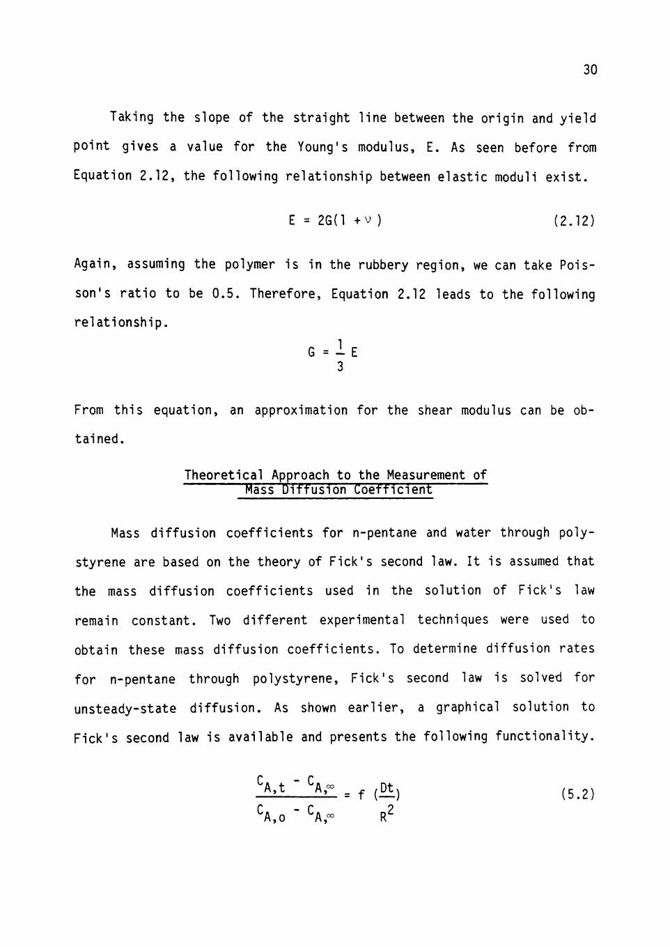
Theoretical Approach to the Measurement of Mass Diffusion Coefflclervf

Mass diffusion coefficients for n-pentane and water through poly

styrene are based on the theory of Fick's second law. It is assumed that

the mass diffusion coefficients used in the solution of Fick's law

remain constant. Two different experimental techniques were used to

obtain these mass diffusion coefficients. To determine diffusion rates

for n-pentane through polystyrene, Fick's second law is solved for

unsteady-state diffusion. As shown earlier, a graphical solution to

Fick's second law is available and presents the following functionality.

%LL^-.f{^) (5.2)

S,o " S,- R

31

The quantity (C^^^ - C ^ « , ) / ( C ^ Q ' ^A °° represents the fractional

weight loss of n-pentane. Again, C. . is the instantaneous concentration

of n-pentane in a bead of polystyrene, C ^ ^, the concentration at the

surface of the bead, and C^ Q, the initial n-pentane concentration. An

assumption is made that the mass diffusion coefficient for n-pentane

J:hrough polystyrene is many orders of magnUude smalj er than the mass

diffusion coefficient through air. This implies that n-pentane diffuses

outward from the surface of the bead into surrounding air much faster

than it diffuses through the inside of the bead. Therefore, surface

resistance to convective mass transfer is negligible. Using this assump

tion implies that C« ^ is zero. The initial n-pentane concentration is

determined by subtracting the weight of polystyrene after all the

n-pentane has been removed from the initial weight of the beads. The

instantaneous concentration is obtained upon subtraction of the weight

of the beads at time t from the initial weight of the beads, and again

dividing this quantity by the initial bead weight. Therefore, the frac

tional weight loss, C, ./C» can be represented as follows.

Cft - w^ " w./w^ w^ - w. _iil = _2 L_o=_2 1 (5.3) S,o . 0 - ^0^/% \ - -

Here, w is the original weight of the polystyrene sample, w. the weight 0 ^

at time t, and w^ the weight after sufficient time for all n-pentane to

diffuse from the beads (i.e., no additional weight loss is observed).

The raw data obtained from experiments designed to determine the mass

diffusion coefficient for n-pentane through polystyrene was handled in

32

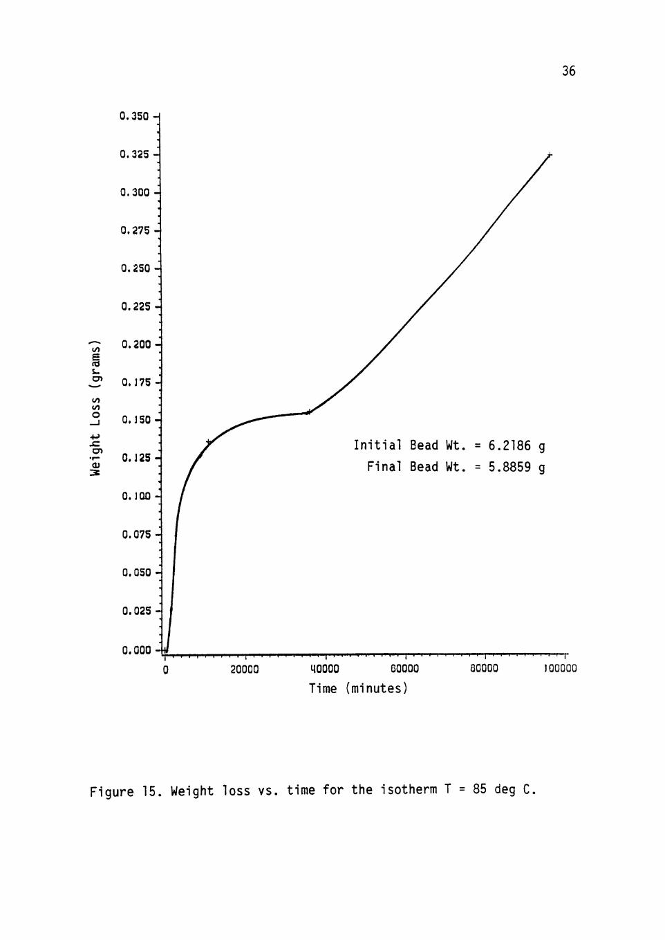
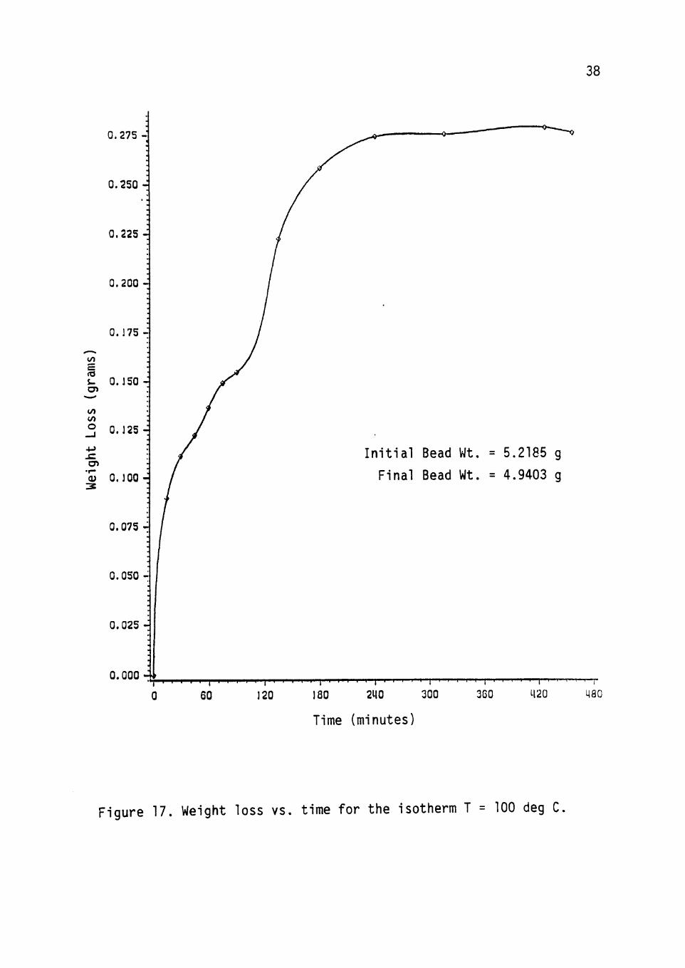
the following manner. Plots of total weight loss versus time were made

for each isotherm of interest. These are shown in Figures 12-19. Next,

the fractional weight loss was calculated based on the data from these

graphs. Now, the plot shown earlier in Figure 4 was used to determine a 2

value for the quantity Dt/R . Since the instantaneous time and radius of

the polystyrene beads were known, a value for the mass diffusion

coefficient could be obtained directly.

In the determination of the mass diffusion coefficient for water

through polystyrene, Fick's second law is solved for steady-state diffu

sion. This solution was shown in Equation 2.19 (Crank, 1968).

j _ = D t . i . 2 _ ^ Ml!!expdPniiii) ^^1 £2 6 ,Z^__^ ^2 ,2

(2.19)

It was assumed that initially, the polymer J;ilm was completely free of

any water. Also, water was continually removed from the low concen

tration side of the film. This suggests that surface resistance to con

vective mass transfer was negligible. A plot of weight loss versus time

was seen to have an x-intercept as seen from Equation 2.21.

t, =— (2.21) ^^9 6D

This is the lag time for water diffusing through a polystyrene film. The

diffusion coefficient can be directly obtained from this equation.

2

6 t D = J- (2.22)

lag

33

U8-1 Q

0.17-^

0 .16 -

Q. IS-

I gra

ms]

Lo

ss

4->

•r—

o.m

Q. 13

0.12

0.11

0.10

0.09

0.06

0.07

0.06

0.05

o . o u -

0 . 0 3 -

0.02

0.01 -I

0.00

I n i t i a l Bead Wt. = 6.6013 g

Final Bead Wt. = 6.2481 g

, [ I I I I I I I •'

0 200000 400000 600000 800000 1000000 1200QQ0

Time (minutes)

Figure 12. Weight loss vs. time for the isotherm T = 50 deg C.

0.22-i

34

E ITS

CO CO

o

• ( - )

en •r— 0)

0 . 2 0 -

0 . 1 8 -

0 . 1 6 -

o . m -

0 . 1 2 -

0 . 1 0 -

0 . 0 8 -

0 . 0 6 -

O . O i l -

0 . 0 2 -

O.OOrt

Initial Bead Wt. = 6.0473 g


I I I I I I I I I I I I I I I 'I I I I I I I I

6000- 12000 18000 2H0Q0 30000 36000 12000

Time (minutes)


35

o.u-j

Q.IO-

0.09-

0.08-

0.07-

-5 0-06 E m

CO CO

o

en •r-

o.os-

O . O H T

0.03-

0.02-i

O.OJ-i

0.00



r I ||| I I I I r I I' I I'l I'l I I I I I I I I I'l I M I I I I I I I I I l " r i r I'l I I I I I I I I • ' I I ' '

2000 4000 6000 6000

Time (minutes)

10000 12000 mOOQ


36

0.350 H

CO

E s-

CO CO

o

JZ CO

•r-(U



0.000-

20000 40000 COOOO

Time (minutes)

60000 JOOOGQ


37

CO

E

OT

CO CO

o

x: OT

0.275'

0.250 -

0.225 -

0.200 -

0.175 -

0 . 1 5 0 -

0.125 -

0 . 1 0 0 -

0 . 0 7 5 -

0.050 -

0.025 -

0.000



500 1000 1500 2000

Time (minutes)

2500 30QQ


38

0.275 -•

0 . 2 5 0 -

0.225 -

0 . 2 0 0 -

0 . 1 7 5 -

co E s- 0 . 1 5 0 ^

CO CO

° 0.125

4J . C OT

Z 0 . 1 0 0 -

0 . 0 7 5 -

0.050 -

0.025 -

0.000

In i t ia l Bead Wt. = 5.2185 g


I I I I I I I I ii I I I I I I I I I I I I I I I I ' " ' I ' I ' I ' l I I

60 1

120 180 2M0 300

Time (minutes)

360 420 ^80


39

0.3S-I

0.00-



TTTT

60 i m m i i i i i m i i i i i i I l l T

70 r

80 90 100 no 120 130

Time (minutes)


40

0.36-



i i i l i i i i i i i i H i i i i i 11II | i i i i i i i i n i i i i i i i i i [ i i i i i i i i i [ I •I • • • • • I I !• 11 1111 I n 111 II 111

5 10 15 20 25 30 35 40 45 50 55 SO

Time (minutes)


41

Plots of weight loss versus time for each isotherm used in obtaining a

mass diffusion coefficient for water through polystyrene are shown in

Figures 20-23.

42

CO

E

CO CO

o

OT

Q.85H

0.60-

0.55

0.50-

0.45-

0.40-

0.35-

0.30-

0.25-

0.20-

0.15-

0.10-

0.05-

0.00-

wt. loss = 0.00853 t - 0.0101

t , = 1.37 hours lag

r I I I I I I I I

0 10

I I I I I I I I I I I I I I I I I I I I I I I I I I I I I I I I

20 30 40 50 60 70 80

Time (hours)

Figure 20. Weight loss of water vs. time for the isotherm T = 50 deg C.

43

CO

OT

OT •r—

0.45-

0.40-

0.35-

0 .30-

^ ' 0.25 H CO CO

o

0.20-

0.15

0.10-

0.05-

0.00-

wt. loss = 0.00955 t - 0.00675

t , = 0.707 hours lag

1 1 1 1 1 1 1 1 1 1 1 1 1 1 1 1 1 1 1 1 1 1 1 1 1 1 1 1 1 1 1 1 1 1 ' 1 1 1 1 1 1 1 1 1

10 20 30 40 50

Time (hours) 60 70 8U


44

wt. loss = 0.0498 t - 0.0145

t, = 0.2482 hours lag 0.0-

10 • ' I '

20 I I I I I T ^ ^ ^ T T - I I I I l l I I

30 40 50

Time (hours) 50 70 80

Figure 22. Weight loss of water vs. time for the isotherm V T = 100 deg C.

Q.SO-I

0.55-

0.50-

45

CO

E s-OT

CO CO

o

OT •r-

0.45-

0.40-

0.35-

0.30-

0.25-

0.20-

0.15-

0.10-

0.05-

0.00-

wt. loss = 0.0631 t - 0.00619

ti = 0.1232 hours lag

1 1 1 1 1 1 1 1 1 1 1 1 1 1 1 1 1 I ' l 1 1 1 1 1 1 1 1 1 1 1 1 ' ' 1 1 1 1 1 1 1 1

10 20 30 40 50

Time (hours) 60 70

I

80


CHAPTER VI

RESULTS OF VISCOSITY MEASUREMENTS

As seen from previous chapters, one part of the objectives for this

study was to determine the viscosity at several different isotherms.

Next, the viscosity data were made to fit a model, which in this case

and for most transport properties is an Arrhenius type of equation.

E^/RT

Here, y^ is a constant with viscosity units, and E is the activation

energy for viscous flow. Taking the natural logarithm of both sides of

Equation 6.1 leads to a linear form of this relationship.

£n y = (- ) 1 + ^n y^ (6.2) R T °

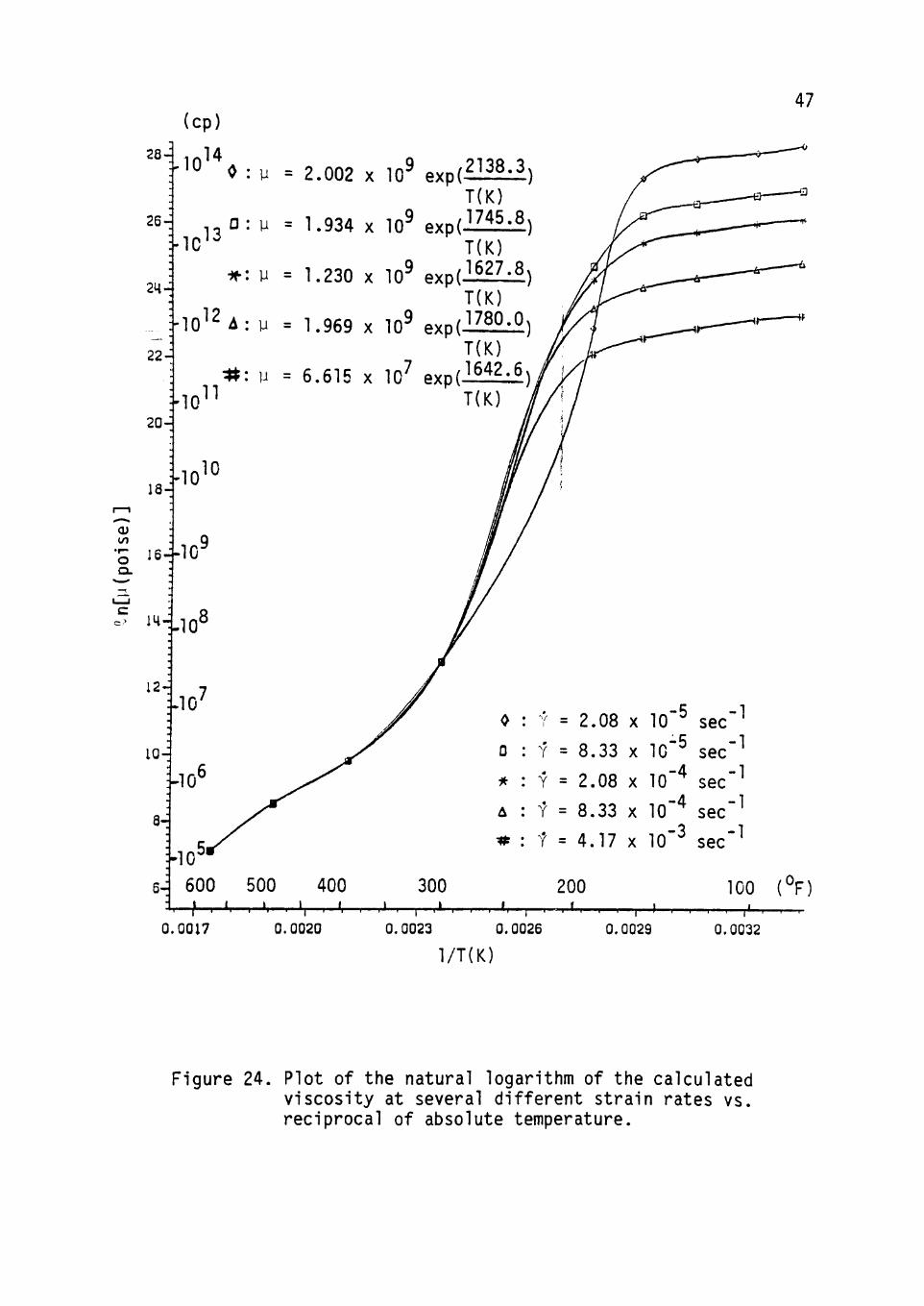
Therefore, a plot of ^n y versus the reciprocal of absolute temperature

leads to a linear curve with slope of E /R and intercept of ^n y . A V 0

plot of the natural logarithm of the calculated apparent viscosity at

several strain rates versus reciprocal of absolute temperature are shown

in Figure 24. With a linear regression of these data, the temperature

dependence on viscosity can be obtained. Since the exponential term in

Equation 6.1 is positive, the viscosity will decrease with a corre

sponding increase in temperature. The results on Figure 24 can be anal

yzed by partitioning the plot into three regions: above the melt temp

erature for polystyrene, below the melt temperature and above the glass

transition temperature, and below the glass transition temperature.

46

47

CO •^• O Q.

28-

26-

24-

22-

20-

18-

1 6 - -

14-

(cp)

,14 0 : y

D : M

• ^ : y =

10^^ A: y

= 2.002 x 10^ e x p ( i M i l T(K)

= 1.934 x 10^ exp(JZl i : i T(K)

= 1.230 X 10^ exp(I§2M T(K)

1.969 X 10^ exp( iZ§M T(K)

6.615 X lO'' exp ( I§ iL l T(K)

12- 7

10-

-1 I r

0.0017 0.0020 0.0023 0.0026

1/T(K)

0.0029 0.0032

Figure 24. Plot of the natural logarithm of the calculated viscosity at several different strain rates vs. reciprocal of absolute temperature.

48

Above the Melt Temperature

Melt viscosities are shown for values of reciprocal of absolute

temperatures less than 0.0024 K~^ (T = 290 deg F). The viscosities in

this temperature region were obtained with the use of a power law rela

tionship which was presented earlier as follows.

T = K Q ( Y ) "

These experimental data were obtained from previous work using a capil

lary rheometer. Based on Figure 24, it is apparent that the melt visco-

si ties are less dependent on strain rate as might be expected based on a

power law fluid model (n < 1.0).

Below the Glass Transition Temperature

Below the glass transition region, the plot of the natural logar

ithm of the apparent viscosity versus the reciprocal of absolute temp

erature can be represented by a straight line for each strain rate val

ue. This is in accord with the Arrhenius equation as shown before. Here,

the magnitude for viscosity increases with a corresponding decrease in

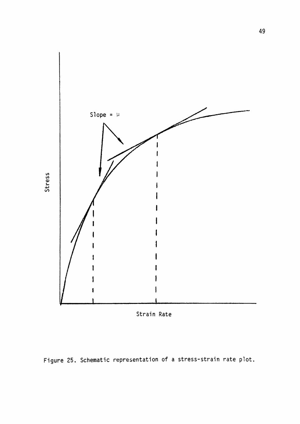
strain rate. This can be interpreted in the following manner. On a

stress-strain plot, as seen in Figure 25, the viscosity is determined by

measuring the slope of a line tangent to the curve (viscosity =

stress/strain rate). For an elastic material under zero shear strain or

stress, the slope of a tangent line will be infinity and a total

resistance to flow results. As the strain rate is increased, the slope

of each tangent line becomes smaller. This results in a corresponding

decrease in viscosity with increasing strain rate.

49

CO CO <u i--p

strain Rate

Figure 25. Schematic representation of a stress-strain rate plot

50

Below the Melt Temperature and Above the Glass iransitjon Temperature

Since there were no experimental data, smooth curves were drawn to

connect the regions above the melt temperature and below the glass

transition temperature (170 deg F to 230 deg F). These curves were used

to represent the apparent viscosity in this region and can be justified

by the restriction that demands this plot be continuous. In Figure 24,

the viscosity measured at a temperature of 190 deg F (1/T(K) = 0.00277)

led to a very peculiar result. The viscosity increased with decreasing

strain rate, as would be expected, until the measurement at the lowest

strain rate showed a decrease in the apparent viscosity. Even though

this datum point seems to be questionable, the reproducibility of the

viscosity value at that temperature and strain rate was within +_ 5

percent. A cursory review of the literature failed to provide a

theoretical explanation for this anomalous behavior. The behavior of the

datum point is therefore unexplained. In this particular region of

Figure 24, the curve for the lowest rate of strain fell well below all

other curves. The curve is represented in this way only to meet the

criterion of continuity. A graph with this peculiar datum point excluded

is shown in Figure 26. Figure 27 represents an overlay of Figures 24 and

26. Experimental data used in the determination of the viscosity of

polystyrene is shown in Appendix A.

51

28-

26-

24-

22-

20-

18-

0) •^ 16-j

o a.

14-

12-

10-

8-

S-I I I I I I I I

0.0017 0.0020 0.0023 0.0026 — ' 1 i ' I < 1 1 r

0.0029 0.0032

1/T(K)

Figure 26. Natural logarithm of apparent viscosity vs. the reciprocal of absolute temperature.

52

CO

o^

20-

26-

24-

22-

20-

18'

1 ''1

14-

12-

10-

8-

S-

0.0017

it-: Y

A : Y

n: Y

= 2.08 x 10"

= 8.33 x 10"

= 2.08 x 10"" sec'

= 8.33 x 10"^ sec'

= 4.17 x 10"^ sec"

• Expected Curve

• I .

0.0020 0.0023 0.0025

1/T(K) 0.0029 0.0032

Figure 27. Natural logarithm of apparent viscosity vs the reciprocal of absolute temperature.

CHAPTER VII

RESULTS OF SHEAR MODULUS MEASUREMENTS

The data obtained in the measurement of shear modulus was, as with

the case of viscosity measurements, made to fit a model described by an

Arrhenius type of equation.

E^/RT 6 = G e ^ (7.1)

0

Here, G is a constant with units of force per unit area, and Eg is the

energy barrier which when crossed causes a loss of ridigity of the

molecules in a material. Again taking the natural logarithms of both

sides of Equation 7.1 leads to a linear form of the relationship.

2,n G = -^ (1) + n G^ (7.2) R T °

A plot of the natural logarithm of the shear modulus versus the

reciprocal of absolute temperature is shown in Figure 28. Here, below

the glass transition temperature the plot is represented by a straight

nearly horizontal line as would be expected since modular properties are

strictly material properties. However, in the glass transition region,

the shear modulus decreases rather rapidly. Again, a smooth curve is

drawn between the data points in this region to maintain continuity.

Experimental data used in the determination of the shear modulus of

polystyrene is shown in Appendix A.

53

54

u -•

10 -

9 -

a -

7 -

6 -

CO

a. ID L—l

5 -

4 ••

2 -

1 -;

0 r

G = 72.29 e x p ( i ! i ^ )

N i l 7 0.00250

I I I I I I I ' l 11111 I I I I I '

0.00265 0.00260 0.00295

1/T(K)

0.00310 0.00325

Figure 28. Natural logarithm of the shear modulus vs the reciprocal of absolute temperature.

CHAPTER VIII

RESULTS OBTAINED FOR MASS DIFFUSION COEFFICIENTS

As was the case for the determination of the viscosity and shear

modulus, the data obtained to determine the temperature dependence of

mass diffusion coefficients for n-pentane and water through polystyrene

were fit to an Arrhenius equation model.

-E /RT D = DQ e ^ (8.1)

2 Here, D is a constant with standard di f fusion units (cm /s) and E, is

0 -— ~—^ L)

the activation energy for diffusion. However, the exponential term in

this equation has a negative value. This represents an increase in the

mass diffusion coefficient with a corresponding increase in temperature.

The results of the calculations for the mass diffusion coefficient of

water through polystyrene are shown in Figure 29. Above and below the

glass transition region, the plot of the natural logarithm of the mass

diffusion coefficient versus the reciprocal of absolute temperature

demonstrated the linear characteristics implied by Equation 8.1. Also,

as was suggested by the Arrhenius equation, the mass diffusion

coefficient increases with increasing temperature. The slopes of the

lines above and below the glass transition region have different values

denoting different activation energies. The slope of the curve in this

Arrhenius plot changes over the glass transition region. The point of

intersection of the lines having different values for the slope is

typically defined as the glass transition temperature.

55

56

u CO

CVJ E CJ

-14.50 -

-14.75 -

-15.00

-15.25

-15.50

-15.75

-16.00

-16,25

-16.50

-16.75

-17.00 -j

-17.25

-17.50

-17.75 -

-18.00

D = 102744.4 exp(ll222)

D = 0.00142 expC^^^^'^)

0.00250 ^ I •! I I I I I I r

0.00265 I I I I I I I I I I I I I I' ' I

0.00280 0.00295 ^

0.00310 0,00323

1/T(K)

Figure 29. Natural logarithm of the mass di f fusion coeff ic ient for water through polystyrene vs. the reciprocal of absolute temperature.

57

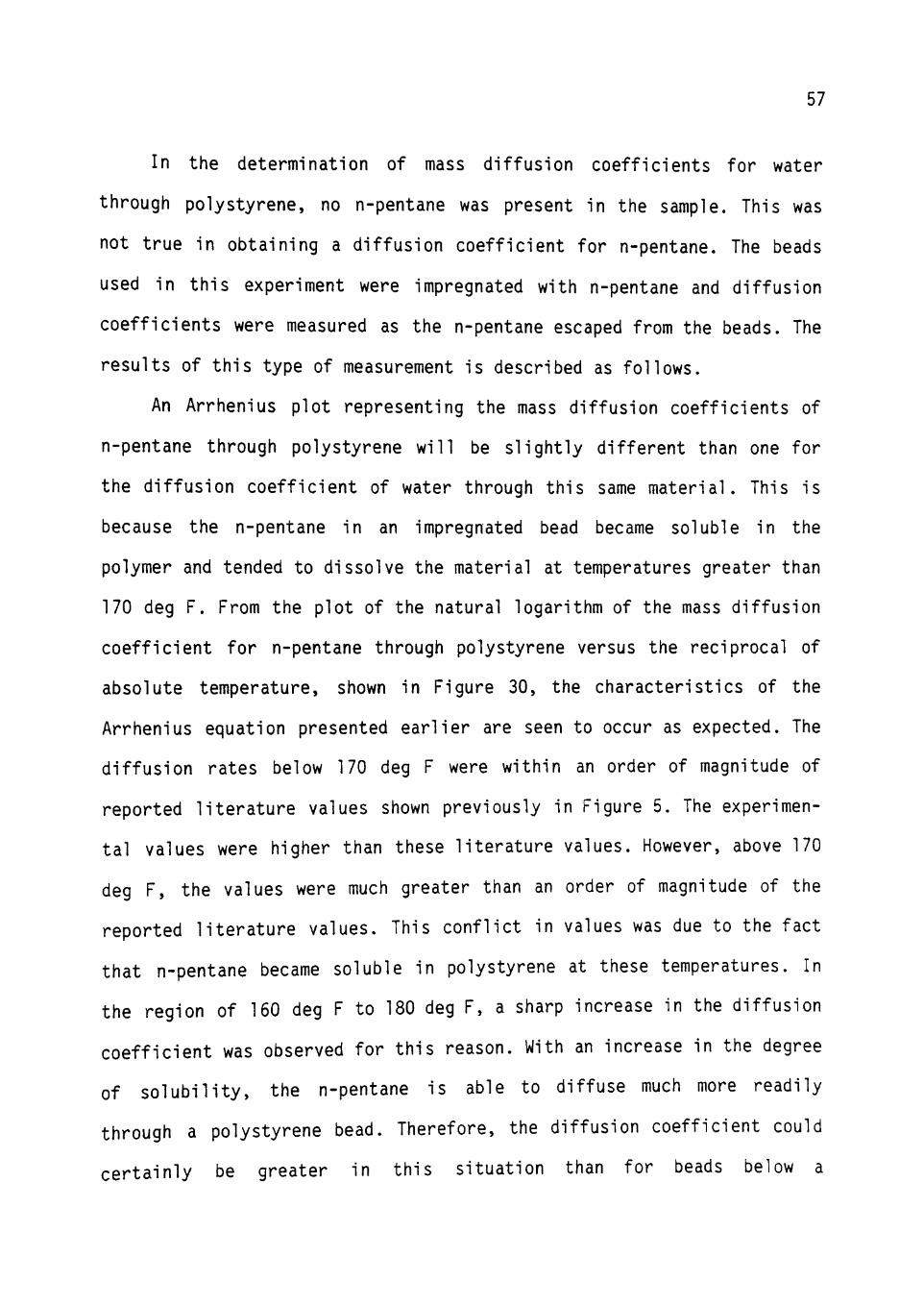
In the determination of mass diffusion coefficients for water

through polystyrene, no n-pentane was present in the sample. This was

not true in obtaining a diffusion coefficient for n-pentane. The beads

used in this experiment were impregnated with n-pentane and diffusion

coefficients were measured as the n-pentane escaped from the beads. The

results of this type of measurement is described as follows.

An Arrhenius plot representing the mass diffusion coefficients of

n-pentane through polystyrene will be slightly different than one for

the diffusion coefficient of water through this same material. This is

because the n-pentane in an impregnated bead became soluble in the

polymer and tended to dissolve the material at temperatures greater than

170 deg F. From the plot of the natural logarithm of the mass diffusion

coefficient for n-pentane through polystyrene versus the reciprocal of

absolute temperature, shown in Figure 30, the characteristics of the

Arrhenius equation presented earlier are seen to occur as expected. The

diffusion rates below 170 deg F were within an order of magnitude of

reported literature values shown previously in Figure 5. The experimen

tal values were higher than these literature values. However, above 170

deg F, the values were much greater than an order of magnitude of the

reported literature values. This conflict in values was due to the fact

that n-pentane became soluble in polystyrene at these temperatures. In

the region of 160 deg F to 180 deg F, a sharp increase in the diffusion

coefficient was observed for this reason. With an increase in the degree

of solubility, the n-pentane is able to diffuse much more readily

through a polystyrene bead. Therefore, the diffusion coefficient could

certainly be greater in this situation than for beads below a

58

-13-1

- 1 4 -

-15

1—1

<J <u CO

C\J E u N _ » «

o

o?

-16

-17

-18

-19

-20

-21

-22

- 2 3 -

- 2 4 -

- 2 5 -

- 2 8 -

- 2 7 -

0.0025Q

D = 2.42 X 10^ exp ( i ! i l l i i i ) T(K)

D = 1.207 X 10'^ eycpilBIlil)

0.00265 0.0028Q 0.00295

1/T(K)

0,00310 Q.G0325

Figure 30. Natural logarithm of the mass diffusion coefficient for n-pentane through polystyrene vs. the reciprocal of absolute temperature.

59

temperature of 170 deg F. In the glass transition region there is not a

great deal of curvature in the data as was evident for the mass

diffusion coefficient of water through polystyrene. Glass transition

temperature does not have as great an effect on diffusion rates for

n-pentane for the following reason. In using an impregnated bead of

polymer during the experimental runs to determine diffusion rates, the

n-pentane has an effect on the glass transition temperature. The

n-pentane tends to plasticize the polystyrene causing the material to

become less rigid in structure. This phenomena leads to a shift in the

region for glass transition. The temperature for glass transition is

essentially lower than the value for pure polystyrene. With this

lowering of the glass transition temperature, the curvature in a plot as

seen previously (Figure 29), is not as great as for polystyrene which

did not contain plasticizers. The glass transition temperature was then

approximately at the same temperature of the large increase of

solubility of n-pentane in polystyrene. This explains why the effect of

glass transition is not as noticeable in this situation. Determining the

mass diffusion coefficients of n-pentane through a bead of polystyrene

which contains a plasticizer is exactly what is needed to fit the

mathematical model used to predict bead density during the prepuffing

operation. However, it is extremely difficult if not impossible to

determine a mass diffusion coefficient for water through polystyrene

which contains the plasticizer n-pentane. This is due to the fact that

for a given mass, one change in the bead's weight cannot be

differentiated between a gain in weight from water entering, or a weight

loss from n-pentane leaving the bead. Experimental data used in the

60

determination of mass diffusion coefficients for water and n-pentane

through polystyrene are shown in Appendix B and C, respectively.

CHAPTER IX

CONCLUSION

The viscosity and mass diffusion coefficients of n-pentane and

water through polystyrene were obtained within an order of magnitude of

the data available from the literature. These transport data were then

utilized in a mathematical model to predict the bead density of

polystyrene during the expansion process. A printout of the computer

program for this model is shown in Appendix D. Predicted bulk bead

density and the pressure drop across the surface of a bead caused by the

n-pentane blowing agent are shown as a function of time.

61

REFERENCES

Brubaker, D. W. and Kammermeyer, K., "Apparatus for Measuring Gas Permeability of Sheet Materials," Anal. Chem., 25, 424-426 (March 1953). —

Brubaker, D. W. and Kammermeyer, K., "Flow of Gases Through Plastic Membranes," Ind. Eng. Chem., 45_, 1148-1152 (May 1953).

Crank, J., Diffusion In Polymers, Academic Press, London, 2-10 (1968).

Deeg, G. and Frosh, C. J., Mod. Plastics, 2£, 155 (1944).

Duda, J. L. and Vrentas, J. S., J. Polymer Sci., [A-2] , 675 (1968).

Hanks, Richard W., Materials Engineering Science, Harcourt, Brace and World, Inc., New York, 22y-23l, 289-293 (19/0).

Hoi ley, R. H., Hopfenburg, H. B., and Stannett, V., "Anomulus Transport of Hydrocarbons in Polystyrene," Polymer Engineering and Science, 20, 376-382 (January 1970).

Landrock and Procter, "Gas Permeability of Films," Modern Packaging, 25, 131-135 (June 1952). "~

Micheals, A. S., et al., J. Appl. Phys., 34, 1 (1963).

Treybal, Robert E., Mass Transfer Operations, McGraw-Hill Book Company, New York, 90-91 (1980).

Van Amerongen, G. J., "Influence of Structure of Elastomers on Their Permeability to Gases," J. Polymer Sci., 5 , 307-332 (1950).

Waack, R., Alex, N. H., Frisch, H. L., Stannet, V., and Szwarc, M., "Permeability of Polymer Films to Gases and Vapors," Ind. Eng. Chem., 47, 2524-2527 (December 1955).

Welty, J. R., Wicks, C. E., and Wilson, R. E., Fundamentals of Momentum, Heat and Mass Transfer, John Wiley and Sons, New York [ 19/bj.

62

APPENDIX A

EXPERIMENTAL DATA FOR VISCOSITY AND SHEAR MODULUS

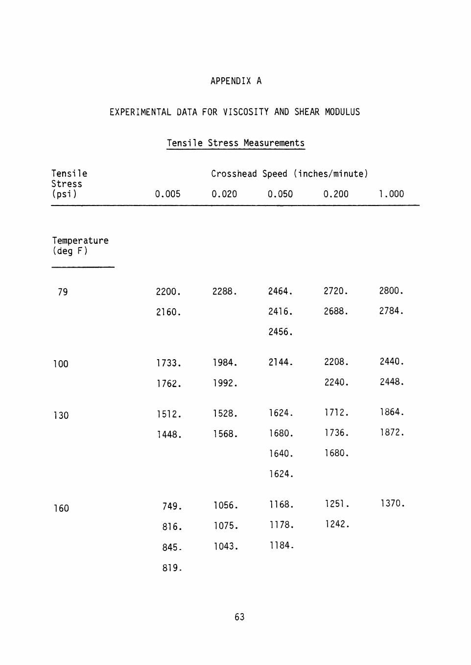
Tensile Stress Measurements

Tensile Crosshead Speed (inches/minute) Stress (psi) 0.005 0.020 0.050 0.200 1.000

Temperature (deg F)

79 2200. 2288. 2464. 2720. 2800.

2160. 2416. 2688. 2784.

2456.

100 1733. 1984. 2144.

160

1733.

1762.

1512.

1448.

1984

1992

1528

1568

130 1512. 1528. 1624.

1680.

1640.

1624,

749.

816.

845-

819.

1056

1075

1043

2208.

2240.

1712.

1736.

1680.

2440.

2448.

1864.

1872.

1168. 1251. 1370.

1178. 1242.

1184.

63

64

Tensile Stress Measurements (continued)

Tensile Crosshead Speed (inches/minute) Stress (psi) 0.005 0.020 0.050 0.200 1.000

Temperature (deg F)

190 6.2 232. 384. 653. 829

386. 666. 842

6.2

4.8

11.4

6.4

13.4

5.8

6.4

14.2

12.0

232

235

65

Viscosity Measurements as a Function of Temperature

and Crosshead Speed

Viscosity (Poise) X EXP(-IO)

Temperature (deg F)

79

100

130

160

190

0.005

240.

193.

163.

89.0

.988

Crosshead

0.020

63.0

54.8

42.6

29.2

6.42

Speed (

0.050

27.0

23.6

18.1

13.0

4.24

!inches/minute)

0.200

7.44

6.12

4.70

3.44

1.81

1.000

1.54

1.35

1.03

.756

-460

66

Viscosity Measurement as a Function of Temperature

and Strain Rate

Ln Viscosity Strain Rate (1/second) x EXP(4) (Viscosity in Poise) 0.208 0.833 2.08 8.33 41.7

1/Temperature (K)

X EXP(3)

3.341 28.506 27.169 26.322 25.033 23.458

3.216 28.289 27.030 26.187 24.837 23.326

3.052 28.120 26.778 25.992 24.537 23.055

2.905 27.514 26.400 25.591 24.261 22.746

2.770 23.014 24.885 24.470 23.619 22.249

67

Shear Modulus as a Function of Temperature

l/Temp(K) x EXP(3) Ln[G(psi)]

3.341 11.389

3.216 11.125

3.052 11.050

2.905 10.661

2.770 10.048

2.673 3.500

APPENDIX B

EXPERIMENTAL DATA FOR MASS DIFFUSION COEFFICIENT

OF WATER THROUGH POLYSTYRENE

Weight Loss of Water as a Function of

Temperature (K)

Temperature and Time

Time (Hours)

24.

48.

72.

12.

24.

48.

6.

9.

12.

7.5

11.5

16.167

Weight L(

0.1948

0.3989

0.6042

0.1068

0.2239

0.4510

0.2851

0.4331

0.5842

0.4677

0.7240

1.0107

323.

323.

323.

353.

353.

353.

373.

373.

373.

383.

383.

383.

68

69

Mass Diffusion Coefficient for Water Through Polystyrene

as a Function of Temperature

1/Temperature (K) Ln[D(Cm**2/sec)]

0.003248 -17.63

0.003094 -16.97

0.002864 -16.31

0.002680 -15.26

0.002610 -14.56

APPENDIX C

EXPERIMENTAL DATA FOR MASS DIFFUSION COEFFICIENT

OF N-PENTANE THROUGH POLYSTYRENE

Fractional Weight Loss of n-Pentane Through Polystyrene

as a Function of Time, Temperature, and the Quantity

Dt/R**2

Temp (deg C)

50.0

75.0

80.0

85.0

90.0

Time (min)

3780.0

8100.0

4010.0

6000.0

6060.0

90.0

420.0

1645.0

120.0

1360.0

360.0

1800.0

Fractional Loss of n-

0.773

0.699

0.649

0.537

0.499

0.730

0.461

0.180

0.624

0.195

0.478

0.114

Weight Pentane Dt/R**2

0.004

0.010

0.011

0.024

0.031

0.006

0.035

0.120

0.018

0.136

0.036

0.187

70

71

Fractional Weight Loss of n-Pentane Through Polystyrene

as

Temp (deg C)

100.0

110.0

120.0

a Function of Time,

Dt/R**

Time (min)

15.0

30.0

45.0

60.0

75.0

17.0

32.0

47-0

62.0

15.0

30.0

Temperature, and

•2 (continued)

the QL

Fractional Loss of n-

0.679

0.592

0.562

0.510

0.464

0.317

0.1919

0.040

0.033

0.063

0.002

Wei Pent

lanti ty

ght :ane Dt/R**2

0.012

0.020

0.026

0.030

0.038

0.068

0.183

0.275

0.295

0.224

0.600

72

Mass Diffusion Coefficient as a

Function of Temperature

1/Temperature (K) Ln[D(Cm**2/sec)]

0.002544 -13.20

0.002610 -14.44

0.002680 -16.56

0.002754 -17.39

0.002792 -18.11

0.002832 -18.66

0.002872 -25.59

0.003094 -26.42

0.003143 -26.57

0.003193 -26.71

0.003299 -27.02

APPENDIX D

COMPUTER PROGRAM FOR MATHEMATICAL MODEL TO PREDICT BEAD

DENSITY OF POLYSTYRENE DURING THE

EXPANSION PROCESS

$JOB DIMENSION ROdOO) ,T(100) ,DO(100) ,DT(100) DIMENSION DKIOO) ,XLNT(100) ,XLNRO(10 0) ,XNI(100) ,XPI(100) TEMP=6 70.

C TEMPERATURE IN DEGREE RANKINE R=1545.

C IDEAL GAS CONSTANT, R, IN (PSF)(FT**3)/(LBM)(DEG R) XP0=2880.

C INITIAL OUTSIDE PRESSURE, XPO, IN PSF U=2087000.

C VISCOSITY, U, IN PSF*SEC XMI=0.000004852

C INITIAL MASS OF BEAD, XMI, IN LBM DDI=0.0000521

C DISTANCE 'INCREMENT, DDI, IN FEET DI(1)=0.000521

C INITIAL INSIDE DIAMETER OF BEAD, DI(1), IN FEET DO(11=0.00521

C INITIAL OUTSIDE DIAMETER OF BEAD, D0(1), IN FEET DT(1)=0.0

C INITIAL TIME INCREMENT, DT(1), IN SECONDS T(1)=0.0

C INITIAL TIME, T(l), IN SECONDS RO(1)=XMI/DO(1)**3. XN1=0.000000005657 XNH20=0.0 XNP0=0.0 DO 10 1=1,50 XNI (I)=XN1+XNH20-XNP0 A=3*XNI(I)*R*TEMP/(U*D0(1)* 3. 1416) B=XP0*D0(I)**2.*( (D0(I)**3.-D0(1)**3.)**(l./3.) ) /(2.*U*DG(1) ) DT(I + 1) = (DI(I) *DDI)/(A-B) T(I + 1)=T(I)+DT(I + 1) XI=(XNH20+0.0 0 00 000016156)/XNI(I) XPI(I)=13725.*XNI(I)/(DI(I)**3.) C=(3.1416*D0(I)**2.)/(DO(I)-DI(I)) XNH20=0.000000010847*C*DT(I + 1)*(20.-XI*XPI(I) ) XNP0=C*(1-XI)*XPI (I)*DT(I + 1)*0.000000000011 IF (0. 0000000016156. LE.ABS(XJ^H20) )XNH20 = 0.0 IF(0.0 000 0 0004 0414.LE.XNPO)XNPO=0.0 D0(I+1)=(D0(1)**3.+DI(I)**3.)**(l./3.) RO(H-1)=XMI/DO(I + 1) **3. DI(I + 1)=DI(I)+DDI

10 CONTINUE WRITE(6,3)

3 FORMATCl' ,/////,6X, • DENSITY (LBM/FT* * 3 ) ' ,4X, ' TIME ( SECONDS ) ' ,//) DO 100 J=l,40 WRITE(6,20)RO(J),T(J)

20 FORMAT(2F20.8) 100 CONTINUE

DO 15 K=l,50 IF(R0(K).LE.O.)G0 TO 16

73

74

I F ( T ( K ) . L E . O . ) G 0 TO 16 XLNR0(K)=AL0G(R0(K)) XLNT(K)=ALOG(T(K)) I F ( R 0 ( K ) . G T . O . ) G 0 TO 15 I F ( T ( K ) . G T . O . ) G O TO 15

16 XLNRO(K)=0.0 17 XLNT(K)=0.0 15 CONTINUE

WRITE(6,2) 2 FORMAT('1',9X,'LN DENSITY',llX,'LN TIME',8X,'INTERN PRES(PSF)',//)

DO 81 1=1,4 0 WRITE(6,82)XLNRO(I),XLNT(I),XPI(I)

82 FORMAT(3F20.8) 81 CONTINUE

STOP END

$ENTRY

75

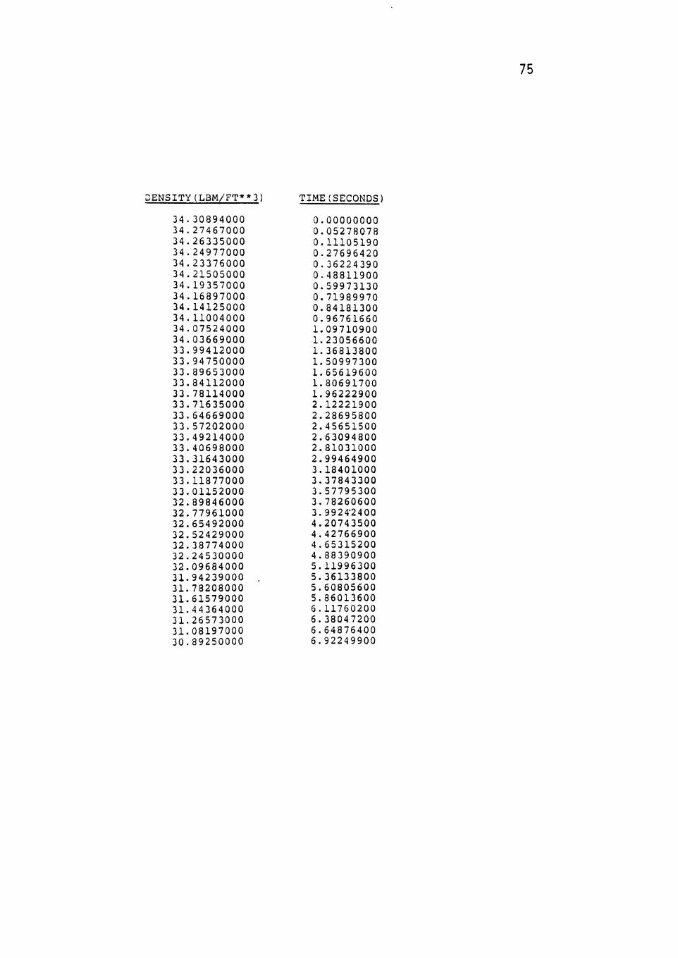
DENSITY(LBM/FT**3) TIME(SECONDS)

34.30894000 0.00000000 34.27467000 0.05278078 34.26335000 0.11105190 34.24977000 0.27696420 34.23376000 0.36224390 34.21505000 0-48811900 34.19357000 0.59973130 34.16897000 0.71989970 34.14125000 0.84181300 34.11004000 0.96761660 34.07524000 1.09710900 34.03669000 1.23056600 33.99412000 1.36813800 33.94750000 1.50997300 33.89653000 1.55619600 33.84112000 1.80691700 33.78114000 1.96222900 33.71635000 2.12221900 33.64669000 2.28695800 33.57202000 2.45651500 33.49214000 2.63094800 33.40698000 2.81031000 33.31643000 2.99464900 33.22036000 3.18401000 33.11877000 3,37843300 33.01152000 3.57795300 32.89846000 3.78260600 32.77961000 3.9924'2400 32.65492000 4.20743500 32.52429000 4.42766900 32.38774000 4.65315200 32.24530000 4.88390900 32.09684000 5.11996300 31.94239000 5.36133800 31.73208000 5.60805600 31.61579000 5.86013600 31.44364000 6.11760200 31.26573000 6.38047200 31.08197000 6.64876400 30.89250000 6.92249900

76

LN DENSITY LN TIME INTERN PRES(PSF!

0.00000000 0.00000000 549016.00000000 3.53440600 -2.94160700 412484.20000000 3.53407500 -2.19775600 122562.60000000 3.53367900 -1.28386500 202154.90000000 3.53321100 -1.01543700 118402.10000000 3.53266500 -0.71719590 116220.60000000 3.53203600 -0.51127330 94929.62000000 3.53131700 -0.32864320 82898.68000000 3.53050600 -0.17219730 71677.18000000 3.52959100 -0.03291926 62514.69000000 3.52857000 0.09267926 54759.95000000 3.53743900 0.20747420 48197.00000000 3.52618600 0.31345080 42608.30000000 3.52481400 0.41209200 37825.91000000 3.52331200 0.50452370 33713.84000000 3.52167600 0.59162210 30161.97000000 3.51990200 0.67408130 27080.49000000 3.51798200 0.75246220 24395.94000000 3.51591400 0.82722280 22047.81000000 3.51369200 0.89874370 19986.10000000 3.51131000 0.96734420 18169.24000000 3.50876400 1.03329400 16562.58000000 3.50605000 1.09682600 15137.08000000 3.50316200 1.15814100 13868.27000000 3.50010000 1.21741100 12735.55000000 3.49685500 1.27479000 11721.35000000 3.49342500 1.33041200 10810.75000000 3.48980600 1.38439800 9991.04200000 3.48599500 1.43685200 9251.26100000 3.48198600 1.48787300 8581.99600000 3.47777900 1.53754400 7975.13200000 3.47337100 1.58594500 7423.62100000 3.46875700 1.63314700 6921.35100000 3.46393300 1.67921300 6462.99600000 3.45890200 1.72420400 6043.88600000 3.45365600 1.76817200 5659.95300000 3.44819600 1.81116900 5307.60100000 3.44252200 1.85324100 4983.67100000 3.43662700 1.89443000 4685.37500000 3.43051300 1.93477600 4410.23000000

transport properties of polystyrene above and a …

Documents