Newton’s, Fourier’s and Fick’s laws Newton’s, Fourier’s and Fick’s laws (Chapters 1, 9, 17)(Chapters 1, 9, 17)

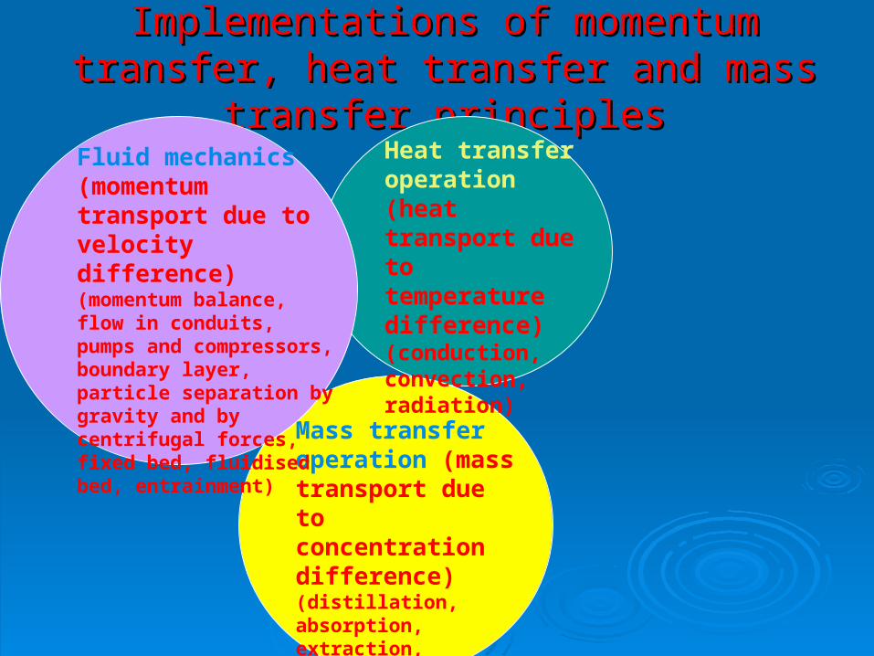
Implementations of momentum transfer, Implementations of momentum transfer, heat transfer and mass transfer principlesheat transfer and mass transfer principles

Momentum transfer

Heat transfer operation (heat transport due to temperature difference) (conduction, convection, radiation)

Mass transfer operation (mass transport due to concentration difference) (distillation, absorption, extraction, humidification)

Fluid mechanics (momentum transport due to velocity difference) (momentum balance, flow in conduits, pumps and compressors, boundary layer, particle separation by gravity and by centrifugal forces, fixed bed, fluidised bed, entrainment)

Mass transport

heat transport

Momentum transport

Boundary layer induces higher velocity gradient close to the inner Boundary layer induces higher velocity gradient close to the inner wall of the pipe. Higher velocity gradient corresponds to higher shear wall of the pipe. Higher velocity gradient corresponds to higher shear stress where more dynamic pressure is converted to heat and stress where more dynamic pressure is converted to heat and consequently higher pump energy is required.consequently higher pump energy is required.

Newton’s law on viscosity

MOMENTUM TRANSPORTMOMENTUM TRANSPORTvelocity velocity in fluid inside the pipein fluid inside the pipe

Momentum Momentum transfer, where transfer, where faster molecules faster molecules will diffuse will diffuse across an area across an area below and impart below and impart their kinetic their kinetic energy energy to slower to slower moleculesmolecules

Smaller pipe Smaller pipe higher average higher average velocity velocity for a for a given volumetric given volumetric flowrateflowrate

Higher velocity Higher velocity incurs higher incurs higher velocity gradientvelocity gradient near the pipe wall, near the pipe wall, which consequently which consequently increases pump increases pump power and vice power and vice versaversa

MASS MASS TRANSPORT TRANSPORT of ink in waterof ink in waterby diffusion by diffusion

due to due to concentrationconcentration

MASS TRANSPORTMASS TRANSPORTconcentrationconcentration in a distillation column in a distillation column

equilibrium curve

operating line

The higher the difference between equilibrium curve and The higher the difference between equilibrium curve and operating line, the larger are loads of condenser and operating line, the larger are loads of condenser and

reboiler, but the smaller the column diameterreboiler, but the smaller the column diameter.

Vapour transfer

liquid transfer

The higher the reflux ratio R (ratio of reflux to distillate product) of the The higher the reflux ratio R (ratio of reflux to distillate product) of the distillation column, the higher is the distillation column, the higher is the concentrationconcentration between equilibrium between equilibrium curve and operating line. This incurs higher utility cost (steam cost). At curve and operating line. This incurs higher utility cost (steam cost). At lower lower RR, column becomes higher (capital cost higher) due to more plates , column becomes higher (capital cost higher) due to more plates required; at higher reflux ratio, column diameter becomes bigger (capital required; at higher reflux ratio, column diameter becomes bigger (capital cost higher). There is an optimised R to get minimum total cost.cost higher). There is an optimised R to get minimum total cost.

temperature temperature in hin heat recovery of heat exchangerseat recovery of heat exchangers

Larger cold utility load at larger ∆T

Larger hot utility load at larger ∆T

Reduced Reduced temperature temperature increased heat recovery (more heat from hot stream is increased heat recovery (more heat from hot stream is given to cold stream) given to cold stream) reduced both hot and cold utilities and vice versa, but reduced both hot and cold utilities and vice versa, but increased area of heat transfer.increased area of heat transfer.

Heat recovery at larger ∆T

Heat recovery at smaller ∆T

Heat transfer

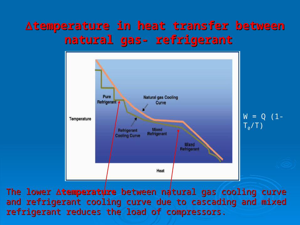
temperature in heat transfer between ntemperature in heat transfer between natural atural gas- refrigerantgas- refrigerant

The lower The lower temperaturetemperature between natural gas cooling curve and refrigerant between natural gas cooling curve and refrigerant cooling curve due to cascading and mixed refrigerant reduces the load of cooling curve due to cascading and mixed refrigerant reduces the load of compressors.compressors.

W = Q (1- T0/T)

Momentum transport:Momentum transport:Newton’s Law of ViscosityNewton’s Law of Viscosity

In Fig. 1.1-1 we show In Fig. 1.1-1 we show a pair of large parallel platesa pair of large parallel plates, , each one with area each one with area A, A, separated by a distance separated by a distance YY. In . In the space between them is a fluid-either a gas or a the space between them is a fluid-either a gas or a liquid. liquid.

This system is initially at rest, but at time This system is initially at rest, but at time tt = 0 the = 0 the lower plate is set in motion in the positive lower plate is set in motion in the positive x x direction direction at a constant velocity at a constant velocity V. V.

As time proceeds, As time proceeds, the fluid gains momentum, and the fluid gains momentum, and ultimately the linear steady-state velocity profile ultimately the linear steady-state velocity profile shown in the figure is established.shown in the figure is established.

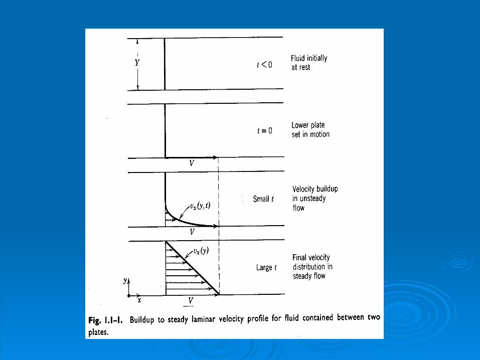
When the final state of steady motion has been When the final state of steady motion has been attained, a constant force attained, a constant force FF is required to maintain is required to maintain the motion of the lower platethe motion of the lower plate. Common sense . Common sense suggests that this force may be expressed as suggests that this force may be expressed as follows:follows: F/A = F/A = V/Y V/Y (1.1-1)(1.1-1)

The force should be The force should be proportional to the area proportional to the area AA and and to the velocityto the velocity, and , and inversely proportional to the inversely proportional to the distance between the platesdistance between the plates. .

The constant of proportionality The constant of proportionality is a property of the is a property of the fluid, defined to be the fluid, defined to be the viscosityviscosity..

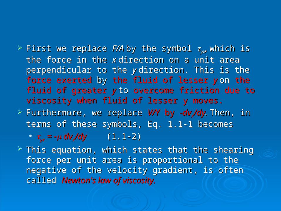
First we replace First we replace F/A F/A by the symbol by the symbol yxyx, , which is the which is the

force in the force in the x x direction on a unit area perpendicular to direction on a unit area perpendicular to the the y y direction. This is the direction. This is the force exerted force exerted byby the fluid of the fluid of lesser lesser y y onon the fluid of greater the fluid of greater y y toto overcome friction overcome friction due to viscosity when fluid of lesser y moves. due to viscosity when fluid of lesser y moves.

Furthermore, we replace Furthermore, we replace V/YV/Y by by -dv-dvxx/dy/dy. . Then, in Then, in

terms of these symbols, Eq. 1.1-1 becomesterms of these symbols, Eq. 1.1-1 becomes yxyx = - = - dv dvxx/dy/dy (1.1-2)(1.1-2)

This equation, which states that the shearing force per This equation, which states that the shearing force per unit area is proportional to the negative of the velocity unit area is proportional to the negative of the velocity gradient, is often called gradient, is often called Newton's law of viscosity.Newton's law of viscosity.

It has been found that the resistance to flow of all It has been found that the resistance to flow of all gases and all liquids with gases and all liquids with molecular weight < about molecular weight < about 5000 5000 is described by Eq. 1.1-2, and such fluids are is described by Eq. 1.1-2, and such fluids are referred to as referred to as Newtonian fluidsNewtonian fluids. .

Polymeric liquids, suspensions, pastes, slurries, and Polymeric liquids, suspensions, pastes, slurries, and other complex fluids are not described by Eq. 1.1-2 other complex fluids are not described by Eq. 1.1-2 and are referred to as and are referred to as non-Newtonian fluidsnon-Newtonian fluids..

Heat transport:Heat transport:Fourier’s Law of ConductionFourier’s Law of Conduction

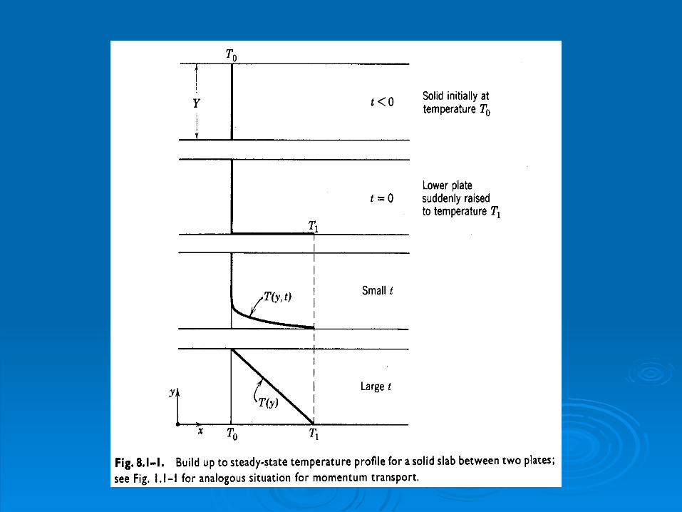
Consider a slab of solid material of area Consider a slab of solid material of area A A located located between two large parallel plates a distance between two large parallel plates a distance YY apart. apart. We imagine that initially (for time We imagine that initially (for time tt < 0) the solid < 0) the solid material is at a temperature material is at a temperature TT00 throughout. throughout.

At At tt = 0 the = 0 the lower plate is suddenly brought to a slightly lower plate is suddenly brought to a slightly higher temperature higher temperature TT11 and maintained at that and maintained at that temperature. temperature.

As time proceeds, the temperature profile in the slab As time proceeds, the temperature profile in the slab changes, and ultimately a linear steady-state changes, and ultimately a linear steady-state temperature distribution is attained (as shown in Fig. temperature distribution is attained (as shown in Fig. 9.1-1).9.1-1).

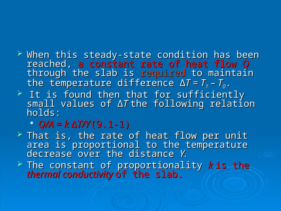
When this steady-state condition has been reached, When this steady-state condition has been reached, a constant rate of heat flow a constant rate of heat flow QQ through the slab is through the slab is requiredrequired to maintain the temperature difference to maintain the temperature difference ∆T = ∆T = TT11 – T – T00. .

It is found then that for sufficiently small values of It is found then that for sufficiently small values of ∆T∆T the following relation holds:the following relation holds: Q/A = k ∆T/YQ/A = k ∆T/Y (9.1-1)(9.1-1)

That is, the rate of heat flow per unit area is That is, the rate of heat flow per unit area is proportional to the temperature decrease over the proportional to the temperature decrease over the distance distance Y.Y.

The constant of proportionality The constant of proportionality k k is the is the thermal thermal conductivity conductivity of the slab.of the slab.

Equation 9.1-1 is also valid if a liquid or gas is placed Equation 9.1-1 is also valid if a liquid or gas is placed between the two plates, provided that suitable between the two plates, provided that suitable precautions are taken precautions are taken to eliminate convection and to eliminate convection and radiation.radiation.

In subsequent chapters it is better to work with the In subsequent chapters it is better to work with the above equation in differential form. That is, we use the above equation in differential form. That is, we use the limiting form of Eq. 9.1-1 as the slab thickness limiting form of Eq. 9.1-1 as the slab thickness approaches zero.approaches zero.

The local rate of The local rate of heat flow per unit area (heat flux) heat flow per unit area (heat flux) in the in the positive positive y y direction is designated by direction is designated by qqyy.. In this notation In this notation Eq. 9.1-1 becomesEq. 9.1-1 becomes

qqyy = - k dT/dy = - k dT/dy (9.1-2)(9.1-2)

This equation, which serves to define This equation, which serves to define k, k, is the one-is the one-dimensional form of dimensional form of Fourier's law of heat Fourier's law of heat conductionconduction. . It states that the heat flux by conduction It states that the heat flux by conduction is proportional to the temperature gradient.is proportional to the temperature gradient.

If the temperature varies in all three directions, then If the temperature varies in all three directions, then we can write an equation likewe can write an equation like

qqxx = - k dT/dx, q = - k dT/dx, qyy = - k dT/dy, q = - k dT/dy, qzz = - k dT/dz = - k dT/dz

(9.1-3, 4, 5)(9.1-3, 4, 5)

If each of these equations is multiplied by the If each of these equations is multiplied by the appropriate unit vector and the equations are then appropriate unit vector and the equations are then added, we get added, we get

. . qq = - k = - k TT (9.1-6)(9.1-6) which is the three-dimensional form of Fourier's law. which is the three-dimensional form of Fourier's law.

Eq. 9.1-2 for each of the coordinate directions.Eq. 9.1-2 for each of the coordinate directions. This equation describes the molecular transport of This equation describes the molecular transport of

heat in isotropic media. By "heat in isotropic media. By "isotropicisotropic" we mean that " we mean that the material has no preferred direction, so that heat the material has no preferred direction, so that heat is conducted with the is conducted with the same thermal conductivity same thermal conductivity k k in in all directionsall directions

Moleculer Mass Transport: Fick‘s Moleculer Mass Transport: Fick‘s Law of Binary DiffusionLaw of Binary Diffusion

Consider a thin, horizontal, Consider a thin, horizontal, fused-silica plate fused-silica plate of area of area A A and thickness and thickness YY. Suppose that initially (for time . Suppose that initially (for time tt < < 0) both horizontal surfaces of the plate are in 0) both horizontal surfaces of the plate are in contact with air, which we regard as completely contact with air, which we regard as completely insoluble in silica. insoluble in silica.

At time At time tt = 0, the air below the plate is suddenly = 0, the air below the plate is suddenly replaced by pure heliumreplaced by pure helium, which is appreciably , which is appreciably soluble in silicasoluble in silica..

The helium slowly penetrates into the plate by virtue The helium slowly penetrates into the plate by virtue of its molecular motion and ultimately appears in the of its molecular motion and ultimately appears in the gas above. gas above.

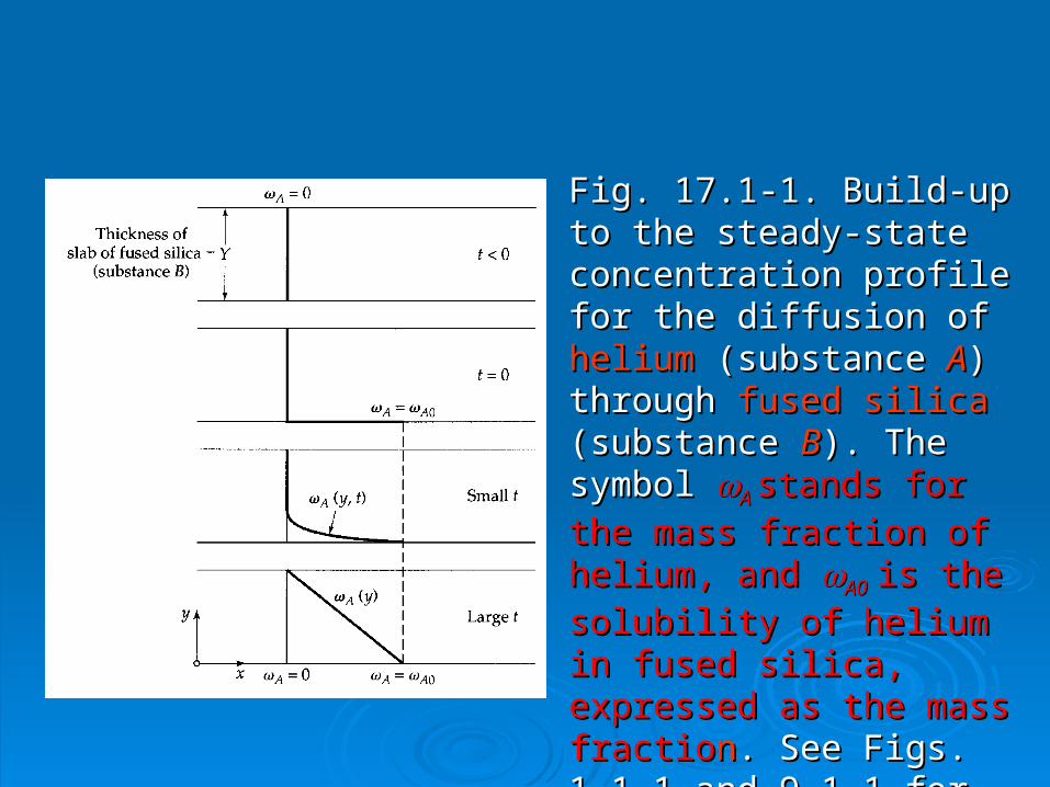
Fig. 17.1-1. Build-up to the Fig. 17.1-1. Build-up to the steady-state concentration steady-state concentration profile for the diffusion of profile for the diffusion of heliumhelium (substance (substance AA) through ) through fused silicafused silica (substance (substance BB). ). The symbol The symbol A A stands for the stands for the

mass fraction of helium, and mass fraction of helium, and A0A0 is the solubility of helium is the solubility of helium

in fused silica, expressed as in fused silica, expressed as the mass fractiothe mass fractionn. See Figs. . See Figs. 1.1-1 and 9.1-1 for the 1.1-1 and 9.1-1 for the analogous momentum and analogous momentum and heat transport situations.heat transport situations.

In this system, we will call In this system, we will call helium "species helium "species A"A" and and silica "species silica "species B"B"

The concentrations will be given by the The concentrations will be given by the "mass "mass fractions" fractions" AA and and BB. .

The mass fraction The mass fraction AA is the mass of helium divided is the mass of helium divided

by the mass of helium plus silica in a given by the mass of helium plus silica in a given microscopic volume element.microscopic volume element.

The mass fraction The mass fraction BB is defined analogously.is defined analogously.

For time t < 0, the mass fraction of helium, For time t < 0, the mass fraction of helium, AA, , is is everywhere equal to zero. everywhere equal to zero.

For time t > 0, at the lower surface, For time t > 0, at the lower surface, y y = 0, the mass = 0, the mass fraction of helium is equal to fraction of helium is equal to A0A0. . This latter quantity This latter quantity is the solubility of helium in silica, expressed as is the solubility of helium in silica, expressed as mass fraction, just inside the solid.mass fraction, just inside the solid.

As time proceeds the mass fraction profile develops, As time proceeds the mass fraction profile develops, with with AA = = A0A0 at the bottom surface of the plate and at the bottom surface of the plate and A A = 0 at the top surface of the plate.= 0 at the top surface of the plate.

As indicated in Fig. 17.1-1, the profile tends toward As indicated in Fig. 17.1-1, the profile tends toward a straight line with increasing a straight line with increasing tt..

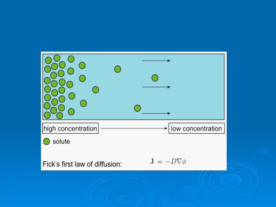
This This molecular transport molecular transport of one substance relative to of one substance relative to another is known as another is known as diffusiondiffusion (also known as (also known as mass mass diffusion, concentration diffusion, diffusion, concentration diffusion, or or ordinary ordinary diffusion).diffusion).

We thus have the situation represented in Fig. 17.1-We thus have the situation represented in Fig. 17.1-1; 1; this process is analogous to those described in this process is analogous to those described in Fig. 1.1-1 and Fig. 9.1-1 where viscosity and Fig. 1.1-1 and Fig. 9.1-1 where viscosity and thermal conductivity were definedthermal conductivity were defined.

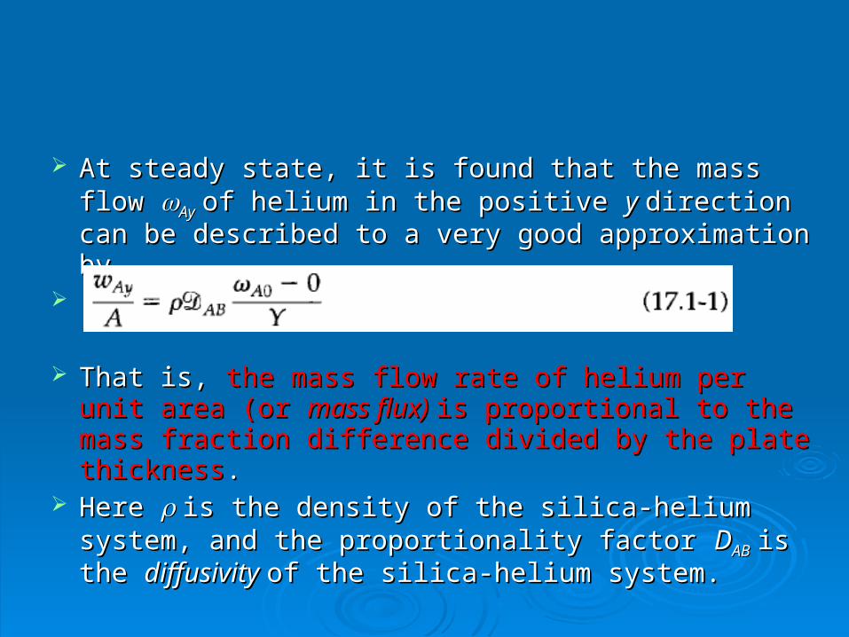
At steady state, it is found that the mass flow At steady state, it is found that the mass flow AyAy of of helium in the positive helium in the positive y y direction can be described to direction can be described to a very good approximation bya very good approximation by

..

That is, That is, the mass flow rate of helium per unit area (or the mass flow rate of helium per unit area (or mass flux) mass flux) is proportional to the mass fraction is proportional to the mass fraction difference divided by the plate thicknessdifference divided by the plate thickness. .

Here Here is the density of the silica-helium system, and is the density of the silica-helium system, and the proportionality factor the proportionality factor DDABAB is the is the diffusivity diffusivity of the of the silica-helium system.silica-helium system.

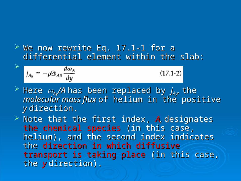
We now rewrite Eq. 17.1-1 for a differential element We now rewrite Eq. 17.1-1 for a differential element within the slab:within the slab:

..

Here Here AyAy/A /A has been replaced by has been replaced by jjAyAy, , the the molecular molecular mass flux mass flux of helium in the positive of helium in the positive y y direction. direction.

Note that the first index, Note that the first index, AA, , designates designates the chemical the chemical speciesspecies (in this case, helium), and the second index (in this case, helium), and the second index indicates the indicates the direction in which diffusive transport is direction in which diffusive transport is taking placetaking place (in this case, the (in this case, the yy direction).direction).

Equation 17.1-2 is the one-dimensional form of Equation 17.1-2 is the one-dimensional form of Fick's first law of diffusion. Fick's first law of diffusion. It is valid for any binary It is valid for any binary solid, liquid, or gas solution, provided that solid, liquid, or gas solution, provided that jjAyAy is is

defined as the mass flux relative to the mixture defined as the mass flux relative to the mixture velocity velocity vvyy..

For the system examined in Fig. 17.1-1, the For the system examined in Fig. 17.1-1, the helium helium is moving rather slowly and its concentration is very is moving rather slowly and its concentration is very small, so that small, so that vvyy 0 0 during the diffusion process.during the diffusion process.

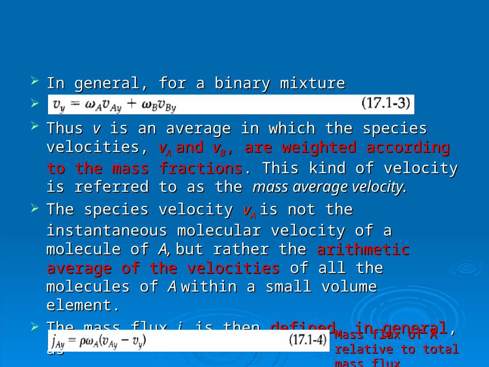
In general, for a binary mixtureIn general, for a binary mixture .. Thus Thus vv is an average in which the species velocities, is an average in which the species velocities,

vvAA and and vvBB, are weighted according to the mass , are weighted according to the mass

fractionsfractions. This kind of velocity is referred to as the . This kind of velocity is referred to as the mass average velocity. mass average velocity.

The species velocity The species velocity vvAA is not the instantaneous is not the instantaneous

molecular velocity of a molecule of molecular velocity of a molecule of A, A, but rather the but rather the arithmetic average of the velocitiesarithmetic average of the velocities of all the of all the molecules of molecules of A A within a small volume element.within a small volume element.

The mass flux The mass flux jjAyAy is then is then defined, in generaldefined, in general, as, asMass flux of A relative to Mass flux of A relative to total mass fluxtotal mass flux

The mass flux of B is defined analogously. The mass flux of B is defined analogously. As the two chemical species interdiffuse there is, As the two chemical species interdiffuse there is,

locally, locally, a shifting of the center of mass a shifting of the center of mass in the in the y y direction if the molecular weights of direction if the molecular weights of A A and B differ. and B differ.

The mass fluxes The mass fluxes jjAyAy and and jjByBy are so defined that are so defined that jjAyAy + + jjByBy = 0. In other words, the fluxes = 0. In other words, the fluxes jjAyAy and and jjByBy are are measured with respect to the motion of the center of measured with respect to the motion of the center of mass (mass (motion of total mass, motion of total mass, vvyy). ).

If we write equations similar to Eq. 17.1-2 for the If we write equations similar to Eq. 17.1-2 for the x x and z directions and then combine all three and z directions and then combine all three equations, we get the vector form of equations, we get the vector form of Fick's lawFick's law::

. A similar relation can be written for species B:A similar relation can be written for species B: ..

It is shown in Example 17.1-2 that It is shown in Example 17.1-2 that DDABAB = = DDBABA... . Thus Thus

for the pair for the pair A-B, A-B, there is just one diffusivity; in there is just one diffusivity; in general it will be a function of pressure, general it will be a function of pressure, temperature, and composition.temperature, and composition.

The mass diffusivity The mass diffusivity DDABAB,, the thermal diffusivity the thermal diffusivity = =

k/(k/(Cp),Cp), and the momentum diffusivity (kinematic and the momentum diffusivity (kinematic viscosity) viscosity) = = // all have dimensions of (length all have dimensions of (length22I I time). time). The ratios of these three quantities are The ratios of these three quantities are therefore dimensionless groups:therefore dimensionless groups:

These dimensionless groups of fluid properties play These dimensionless groups of fluid properties play a prominent role in dimensionless equations for a prominent role in dimensionless equations for systems in which systems in which competing transport processes competing transport processes occuroccur

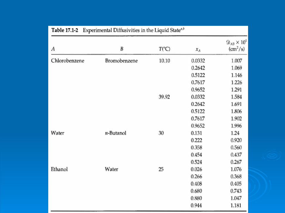
In Tables 17.1-1, 2, 3, and 4 some values of In Tables 17.1-1, 2, 3, and 4 some values of DDABAB in in cmcm22/s /s are given for a few gas, liquid, solid, and are given for a few gas, liquid, solid, and polymeric systems. These values can be converted polymeric systems. These values can be converted easily to measily to m22/s/s by multiplication by 10 by multiplication by 10-4-4

Diffusivities of gases Diffusivities of gases at low density are almost at low density are almost independent of independent of AA, , increase with temperatureincrease with temperature, and , and vary vary inversely with pressureinversely with pressure. .

Liquid and solid diffusivitiesLiquid and solid diffusivities are strongly are strongly concentration-dependent and concentration-dependent and generally increase generally increase with temperature.with temperature.